Diffusion of a particle via a stochastic process on the Pascal’e pyramid.

Abstract

In this note, we construct a $3$-dimensional generalisation of the Pascal’s triangle that we named Pascal’s cube, as it has the construction of a cube with entries given by extended binomial coefficients ${}^{c}C^{a}_{b}$. The Pascal’s cube is equivalent to the well-studied Pascal’s pyramid, with the advantage that the Pascal’s cube can be mapped onto the Cartesian plane for easier computation.

We define a stochastic process using extended binomial coefficients on the Pascal’s pyramid representing the dispersion of a free particle. With some constrains, we showed that this stochastic process satisfies the heat equation.

1 Introduction

A stochastic process is a rule for assigning every experimental outcome a function $P(x,t)$, which gives rise to a family of time functions depending on the position $x$ [1]. Brownian motion and random walks are examples of a stochastic process.

It has been of great interest to connect quantum mechanics to a stochastic theory of Physics. For instance, [2] is an attempt to link the Schrödinger equation to a Markov process, which is a stochastic process in $6$ dimension hypothesised for the motion of a particle.

Since the Pascal’s triangle is well-known to present the possibility of random walks on a $2$-dimensional coordinate [3], it is intriguing to find a connection between the Pascal’s triangle and quantum mechanics. For instance, [4] introduced a generalisation of the classical Pascal’s triangle and presented a link between a stochastic process and quantum mechanics.

In this paper, we present a link between a stochastic process via the Pascal’s pyramid, a higher dimensional generalisation of the Pascal’s triangle and heat equation. Since the heat equation is equivalent to the Schrödinger equation with a wick rotation in time, there could be a possible connection between stochastic processes on the Pascal’s pyramid and quantum mechanics.

This paper is organised as follows. In section 2, we construct Pascal’s cube, a variation of the Pascal’s pyramid with entries denoted by extended binomial coefficients ${}^{c}C^{a}_{b}$ which can be computed using binomial coefficients. In section 3 we maps the Pascal’s cube to the Pascal’s pyramid. In section 4, a stochastic process $P(x,y,t)$ is defined as the probability distribution on the Pascal’s pyramid, describing the dispersion of a particle with time. In section 5, we construct a stochastic process $P(x,t)$ on the Pascal’s pyramid satisfying the heat equation.

2 Pascal’s cube and extended binomial coefficients

In this section, we construct Pascal’s cube and introduce extended binomial coefficients.

2.1 Construction of the Pascal’s cube

Pascal’s triangle, named after the French Mathematician and Philosopher Blaise Pascal [5], is a triangular array of the binomial coefficient arranged by adding the two closest numbers above. Fig 1(a) displays the first $6$ rows of the Pascal’s triangle.

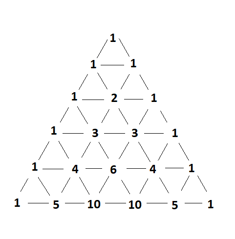
(a) The first $6$ rows of Pascal’s triangle.

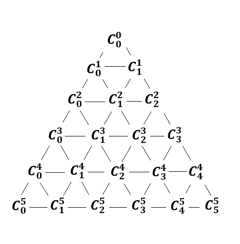
(b) Pascal’s triangle represented by binomial coefficients.

Figure 1: Pascal’s triangle

Pascal’s triangle arises in combinatorics as each entry in the Pascal’s triangle can be represented by a binomial coefficient $C_{k}^{n}$ [5], where $C_{k}^{n}$ is defined by

$$C_{k}^{n}=\frac{n!}{k!(n-k)!}.$$

Thus the Pascal’s triangle can be represented by binomial coefficients as shown in Fig 1(b).

It follows from the definition of the Pascal’s triangle that

$$\left\{\begin{array}[]{ll}C_{0}^{n}&=C^{n}_{n}=1,\\ C_{a}^{n}&=C_{a-1}^{n-1}+C_{a}^{n-1},\end{array}\right.$$ (1)

where $n\geq a+1,a\geq 1$, $n,a\in\mathbb{Z}$.

We then generalise the Pascal’s triangle to $3$-dimensions by adding one dimension perpendicular to the Pascal’s triangle, and each entry is arranged by adding the three closest prior numbers. Let us name the $3$-dimensional generalisation of the Pascal’s triangle a Pascal’s cube, as it takes the shape of a cube. The first three layers of the Pascal’s cube is presented in Fig 2(a).

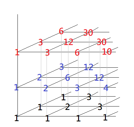
(a) Pascal’s cube represented by numbers.

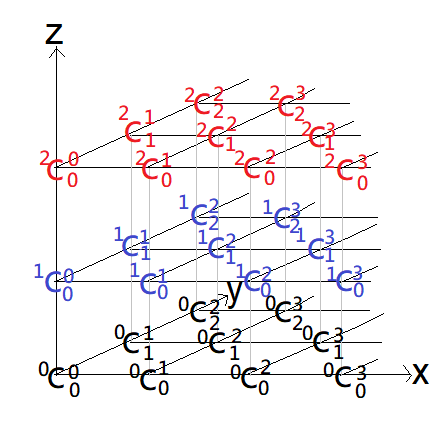
(b) Pascal’s cube represented by extended binomial coefficients.

Figure 2: Pascal’s cube, a three dimensional generalisation of the Pascal’s triangle.

As shown in Fig 2(b), we define elements in the Pascal’s cube by ${}^{c}C_{b}^{a}$, where $a,b,c\in\mathbb{Z}_{+}$. ${}^{c}C_{b}^{a}$ is called an extended binomial coefficient. The base layer of the Pascal’s cube is the original Pascal’s triangle, such that ${}^{0}C^{a}_{b}\equiv C^{a}_{b}$.

Definition 2.1 (Extended binomial coefficient).

As a generalisation of (1), elements in the Pascal’s cube are denoted by ${}^{c}C_{b}^{a}$ and are defined by the following relationships:

$$\left\{\begin{array}[]{ll}{}^{c}C^{0}_{0}&=1,\\ {}^{c}C^{a}_{0}&={}^{c}C^{a-1}_{0}+{}^{c-1}C^{a}_{0},\\ {}^{c}C^{a}_{a}&={}^{c}C^{a-1}_{a-1}+{}^{c-1}C^{a}_{a},\\ {}^{c}C^{a}_{b}&={}^{c}C^{a-1}_{b-1}+{}^{c}C^{a-1}_{b}+{}^{c-1}C^{a}_{b},\end{array}\right.$$ (2)

where $a>b>0$.

Similar to the binomial coefficients, extended binomial coefficients satisfy the following symmetry

$${}^{c}C^{0}_{0} = C^{0}_{0},$$

$${}^{c}C^{a}_{b} = {}^{c}C^{a}_{a-b}.$$

We can put a Cartesian plane on the Pascal’s cube as follows:

Corollary 2.0.1.

Consider the Cartesian coordinate system on the Pascal’s cube as shown in Fig. 2(b). The extended binomial coefficient at a given coordinate $(x,y,z)$ is given by ${}^{z}C^{x+y}_{y}$.

2.2 Extended binomial coefficients

Extended binomial coefficients are entries of the Pascal’s cube satisfying Eqn. 2. In this session, we demonstrate that these coefficients can be computed using the usual binomial coefficients.

For the $c$-th layer, here is a general rule for the extended binomial coefficient:

Theorem 2.1.

$${}^{c}C^{a}_{b} = \sum_{n=0}^{a}\sum_{m=0}^{b}C^{n}_{m}.{}^{c-1}C^{a-n}_{b-m}$$

$$= \prod_{i=0}^{c}\left(\sum_{n_{i}}^{a}\sum_{m_{i}}^{b}C_{m_{i}}^{n_{i}}\right)\times C^{a-n}_{b-m},$$

where $n=\sum_{i=0}^{c}n_{i}$, and $m=\sum_{i=0}^{c}m_{i}$.

With the following restrictions imposing on $n_{i}$ and $m_{i}$:

$$n_{i}\geq m_{i}\geq 0,$$

$$a-(n_{1}+n_{2}+n_{3}+\cdots+n_{c})\geq b-(m_{1}+m_{2}+m_{3}+\cdots+m_{c}),$$

$$0\leq\sum_{i=1}^{c}n_{i}\leq a,\text{and }0\leq\sum_{i=1}^{c}m_{i}\leq b.$$

Proof.

Base case:

$${}^{c}C^{0}_{0} = C^{0}_{0}.C^{0}_{0}=1,$$

$${}^{c}C^{a}_{0} = \sum_{n=0}^{a}C^{n}_{0}.{}^{c-1}C^{a-n}_{0}=\sum_{n=0}^{a}{}^{c-1}C_{0}^{a-n}={}^{c}C^{a-1}_{0}+{}^{c-1}C^{a}_{0},$$

$${}^{c}C^{a}_{a} = {}^{c}C^{a}_{0}.$$

Inductive step: Assuming

$${}^{c}C^{a}_{b}=\sum_{n=0}^{a}\sum_{m=0}^{b}C^{n}_{m}.{}^{c-1}C^{a-n}_{b-m}.$$

Then

$${}^{c}C^{a+1}_{b} = {}^{c}C^{a}_{b-1}+{}^{c}C^{a}_{b}+{}^{c-1}C^{a+1}_{b}$$

$$= \sum_{n=0}^{a}\sum_{m=0}^{b-1}C^{n}_{m}.{}^{c-1}C^{a-n}_{b-1-m}+\sum_{n=0}^{a}\sum_{m=0}^{b}C^{n}_{m}.{}^{c-1}C^{a-n}_{b-m}+\sum_{n=0}^{a+1}\sum_{m=0}^{b}C^{n}_{m}.{}^{c-2}C^{a-n}_{b-m}$$

$$= \sum_{n=0}^{a+1}\sum_{m=0}^{b}C^{n}_{m}\left({}^{z-1}C^{a-n}_{b-1-m}+{}^{c-1}C^{a-n}_{b-m}+{}^{c-2}C^{a-n}_{b-m}\right)$$

$$= \sum_{n=0}^{a+1}\sum_{m=0}^{b}C^{n}_{m}.{}^{c-1}C^{a+1-n}_{b-m}.$$

Thus by mathematical induction, theorem 2.1 holds for all $c\geq 0$. ∎

Following is an example to demonstrate this rule.

Example 2.1.

$${}^{2}C_{2}^{3} = \sum_{n_{1}=0}^{3}\sum_{n_{2}=0}^{3-n_{1}}\sum_{m_{1}=0}^{2}\sum_{m_{2}=0}^{2-m_{1}}C_{m_{1}}^{n_{1}}C_{m_{2}}^{n_{2}}C_{2-m_{1}-m_{2}}^{3-n_{1}-n_{2}}$$

$$= C_{0}^{0}\left(C_{0}^{0}C_{2}^{3}+C_{0}^{1}C_{2}^{2}+C_{1}^{1}C^{2}_{1}+C^{2}_{1}C^{1}_{1}+C^{2}_{2}C^{1}_{0}+C^{3}_{2}C^{0}_{0}\right)$$

$$+ C^{1}_{0}\left(C^{0}_{0}C^{2}_{2}+C^{1}_{1}C^{1}_{1}+C^{2}_{2}C^{0}_{0}\right)+C^{1}_{1}\left(C^{0}_{0}C^{2}_{1}+C^{1}_{0}C^{1}_{1}+C^{1}_{1}C^{1}_{0}+C^{2}_{1}C^{0}_{0}\right)$$

$$+ C^{2}_{1}\left(C^{0}_{0}C^{1}_{1}+C^{1}_{1}C^{0}_{0}\right)+C^{2}_{2}\left(C^{0}_{0}C^{1}_{0}+C^{1}_{0}C^{0}_{0}\right)+C^{3}_{2}C^{0}_{0}C^{0}_{0}$$

$$= 30.$$

3 Mapping Pascal’s cube to Pascal’s pyramid

The Pascal’s pyramid is originally constructed by Staib [6] as a $3$-dimensional generalisation of the Pascal’s triangle. It can be constructed as follows. For the $n$-th layer in the Pascal’s pyramid, take the first $n$ rows of the Pascal’s triangle and multiply each row with elements from the last row. Figure 3 shows the construction of the first five layers.

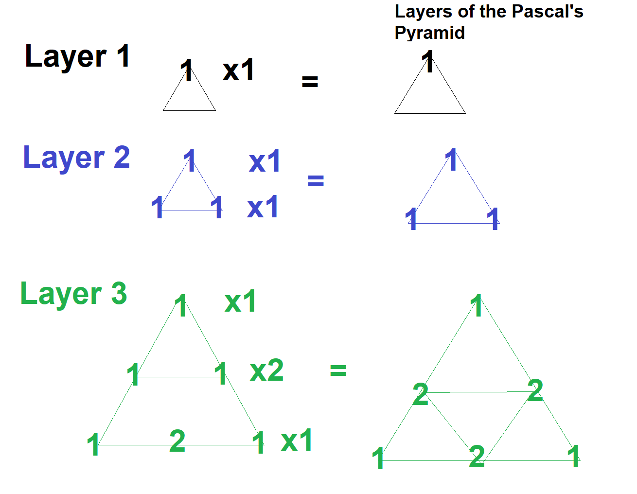
(a) First $3$-layers.

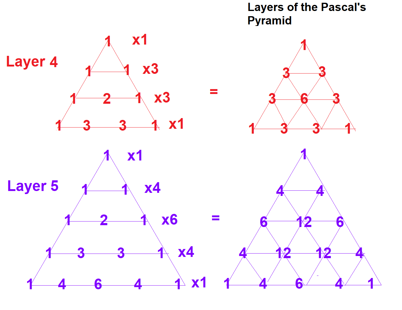
(b) $4$-th and $5$th layers.

Figure 3: Construction of the first $5$ layers of the Pascal’s pyramid.

Figure 4(a) presents the first 5 layers of the Pascal’s pyramid.

Properties of the Pascal’s pyramid include

• There is a three way symmetry in each layer.

• Sum of all numbers in the $n$-th layer is $3^{n-1}$.

We can map layers of the Pascal’s pyramid to the Pascal’s cube. Mapping of the first three layers are shown in Figure 4(b). Each layer of the Pascal’s pyramid becomes a diagonal cross-section in the Pascal’s cube.

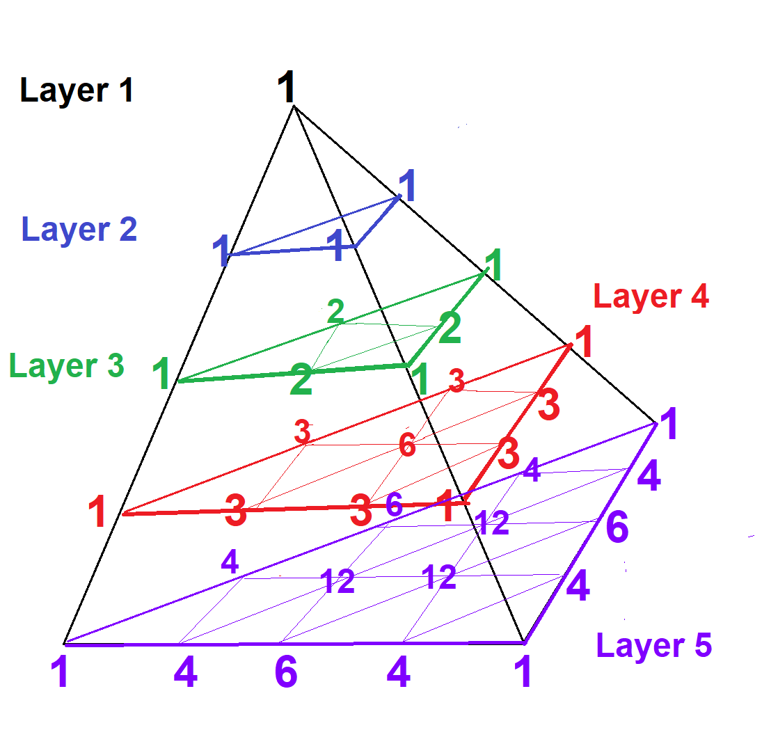
(a) First $5$ layers of the Pascal’s pyramid.

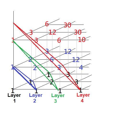
(b) $4$-th and $5$th layers.

Figure 4: Pascal’s pyramid

We now map the layers of the Pascal’s pyramid to the Pascal’s cube and represent elements of the Pascal’s pyramid using generalised binomials. The first $5$ layers are shown in Fig 5.

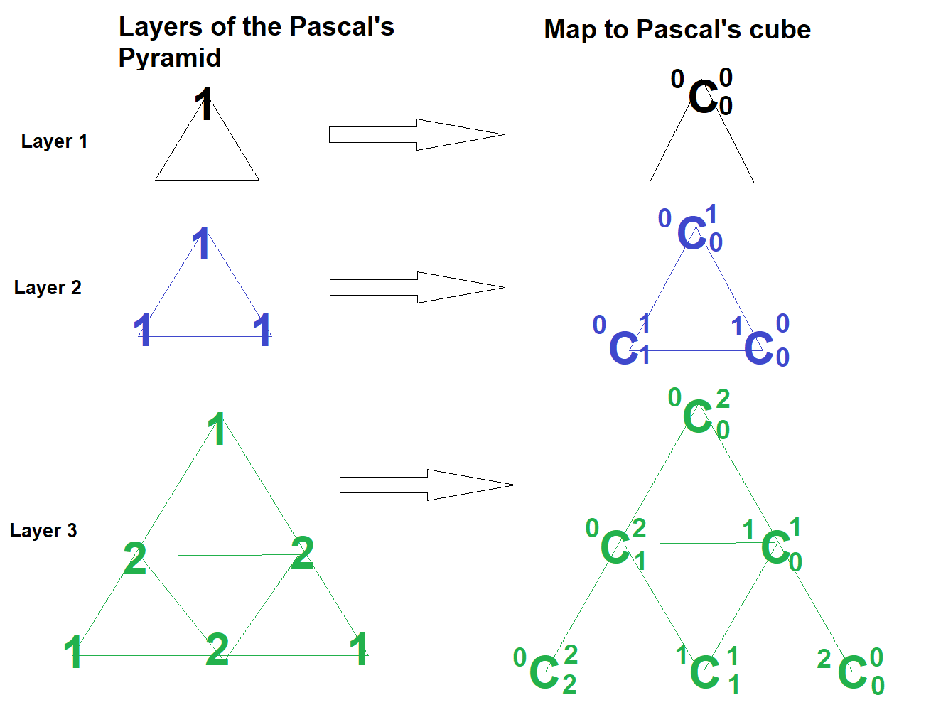
(a) $1$st to $3$rd layer.

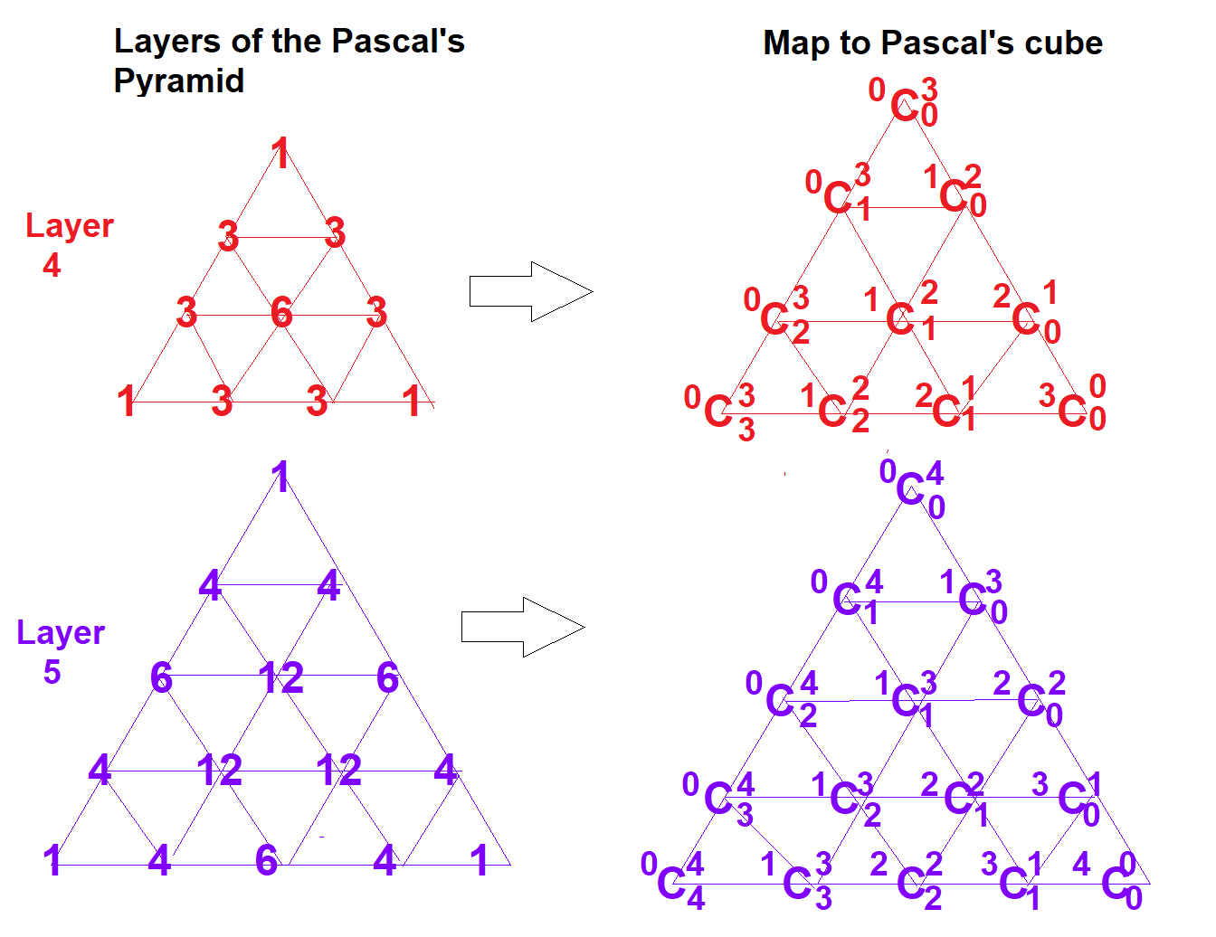
(b) $4$th and $5$th layers.

Figure 5: Mapping generalised binomials to the first $5$ layers of the Pascal’s pyramid.

Theorem 3.1.

By comparing elements in the Pascal’s pyramid with extended binomial coefficients in the Pascal’s cube, we can re-define the extended binomial coefficients using the following relationship:

$${}^{z}C^{x}_{y}=C^{y+z}_{z}\times C^{x+z}_{y+z}.$$ (3)

Eqn. 3 is equivalent to the equation in Theorem 2.1, however Eqn. 3 is much easier to compute with.

4 Probability of a random walk on the Pascal’s pyramid

Let us investigate the dispersion of a particle using the Pascal’s pyramid. Consider the convention that at time $t$, the probability distribution of the particle depends on the extended binomial coefficients on the $3t+1$-th layer of the Pascal’s pyramid, as shown in Fig. 6(a). Fig. 6(b) shows the layers of Pascal’s pyramid corresponding to $t=2$ and $t=3$ in terms of extended binomial coefficients.

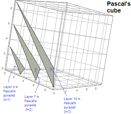
(a) Layers of the Pascal’s pyramid.

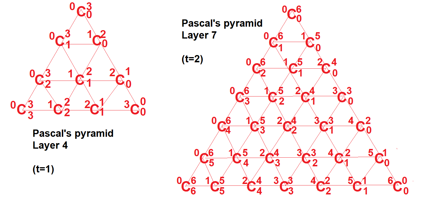
(b) Layer 4 and layer 7 of the Pascal’s pyramid.

Figure 6: Pascal’s pyramid.

We construct a coordinate system on layers of the Pascal’s pyramid where $x$ corresponds to the rows while $y$ corresponds to the columns. Fig. 7 demonstrates coordinate $(x,y)$ on the $4$-th and the $7$-th layers of the Pascal’s pyramid, where the extended binomial coefficient at $(0,0)$ is ${}^{t}C^{2t}_{t}$.

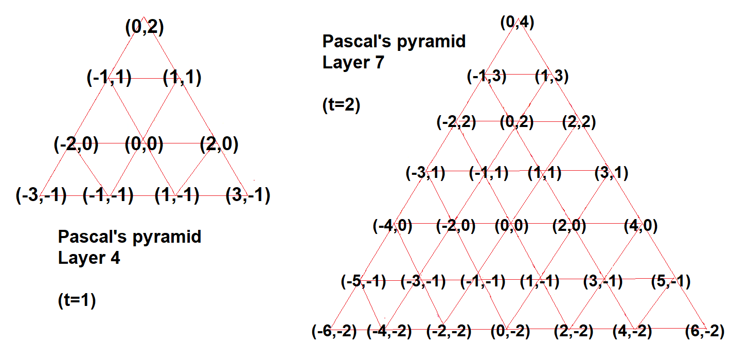
Figure 7: $(x,y)$ coordinate on layer $4$ and layer $7$ of the Pascal’s Pyramid.

The extended binomial coefficient at $(x,y)$ on the $3t+1$-th layer of the Pascal’s pyramid is given by

$${}^{t+\frac{1}{2}(x-y)}C^{2t-\frac{1}{2}(x-y)}_{y+t}.$$

We define a probability function $P(x,y)$ on the $3t+1$-th layer as

$$P(x,y)=\frac{{}^{t+\frac{1}{2}(x-y)}C^{2t-\frac{1}{2}(x-y)}_{y+t}}{3^{3t}},$$ (4)

where the scaling factor $3^{3t}$ is the sum of all entries in the $3t+1$-th layer of the Pascal’s pyramid.

Fig. 8 shows $P(x,y)$, the probability distribution of the particle at $t=1$, $t=2$ and $t=3$.

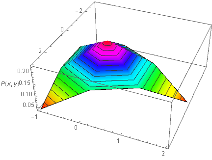
(a) Probability distribution at $t=1$.

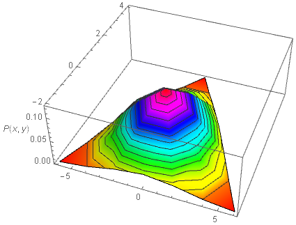
(b) Probability distribution at $t=2$.

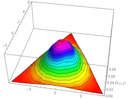
(c) Probability distribution at $t=3$.

Figure 8: Probability distribution of a particle from $t=1$ to $t=3$.

5 Heat equation

Let us define a stochastic process $P(x^{\prime},t)$ on the Pascal’s pyramid, with $t$ corresponds to the $3t+1$-th layer of the Pascal’s pyramid, and $x^{\prime}$ corresponds to the position in the middle row (i.e. $y=0$ and $x^{\prime}=x/2$) as shown in Fig. 9. The extended binomial coefficient corresponds to coordinate $x^{\prime}$ at time $t$ is given by ${}^{t+x^{\prime}}C^{2t-x^{\prime}}_{t}$.

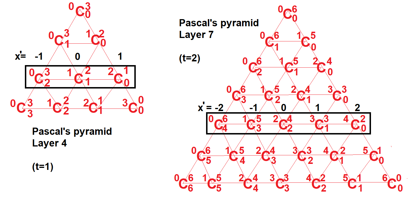
Figure 9: Layer 4 and layer 7 of the Pascal’s pyramid.

Definition 5.1.

Let $P(x^{\prime},t)$ be a discrete-time process defined by

$$P(x^{\prime},t)=\frac{{}^{t+x^{\prime}}C^{2t-x^{\prime}}_{t}}{3^{3t}},$$ (5)

where $-t\leq x\leq t$, and $x^{\prime}\in\mathbb{Z}$.

Fig 10 demonstrates the evolution of $P(x^{\prime},t)$ from $t=2$ to $t=7$.

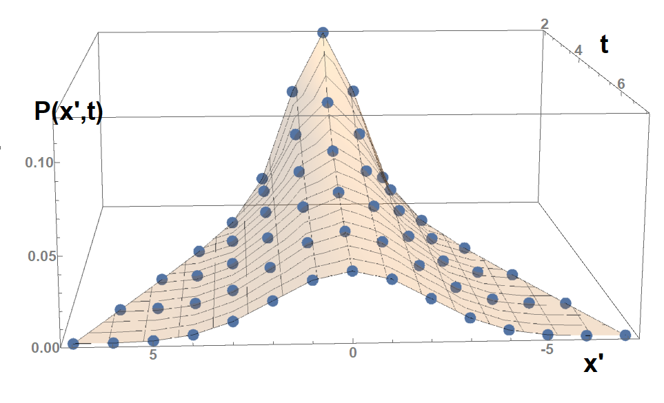
Figure 10: Spreading of $P(x^{\prime},t)$ in the space-time lattice.

Theorem 5.1.

For large $t$ and $t\gg x^{\prime}$, $P(x^{\prime},t)$ satisfies the following diffusion equation:

$$\frac{\partial P(x^{\prime},t)}{\partial t}=\frac{1}{2}\frac{\partial^{2}P(x^{\prime},t)}{\partial x^{\prime 2}},$$ (6)

Proof.

First of all,

$$P(x^{\prime},t)=\frac{{}^{t+x^{\prime}}C^{2t-x^{\prime}}_{t}}{3^{3t}}=\frac{C^{2t+x^{\prime}}_{t+x^{\prime}}\times C^{2t-x^{\prime}}_{t}}{3^{3t}}=\frac{3t!}{(t+x^{\prime})!\times t!\times(t-x^{\prime})!\times 3^{3t}}$$

$P(x^{\prime},t)$ is a discrete function, here we replace $\Gamma(n+1)$ for $n!$ in order to differentiate $P(x^{\prime},t)$:

$$P(x^{\prime},t)=\frac{\Gamma(3t+1)}{\Gamma(t+x^{\prime}+1)\times\Gamma(t+1)\times\Gamma(t-x^{\prime}+1)\times 3^{3t}}.$$

Assuming $t$ is very large and $t\gg x^{\prime}$, then

$$\frac{\partial P(x^{\prime},t)}{\partial t}=P(x^{\prime},t)\times\left(-\frac{1}{2(t+x^{\prime})}-\frac{1}{2(t-x^{\prime})}\right),$$

and

$$\frac{\partial^{2}P(x^{\prime},t)}{\partial x^{\prime 2}}=P(x^{\prime},t)\times\left(-\frac{1}{t+x^{\prime}}-\frac{1}{t-x^{\prime}}\right).$$

Thus $P(x^{\prime},t)$ satisfies Eqn. 6, a heat equation. ∎

6 Conclusion

In this paper, we presented a computationally useful way to explore Pascal’s pyramid, a $3$ dimensional generalisation of the Pascal’s triangle. We constructed a stochastic process that resembles probability distribution of a particle propagating on the Pascal’s pyramid, and showed that with a certain constraint, the stochastic process satisfies the heat equation.

It is well-known that Schrödinger equation can be derived from the heat equation when the time becomes imaginary. However it is unclear if the approach presented here can be applied to the Schrödinger equation. In this paper we proposed a possible way to connect stochastic processes via the Pascal’s pyramid to quantum mechanics.