Appendix:
Consistency and Monotonicity Regularization for Neural Knowledge Tracing

name	logs	students	questions	skills	avg. length	avg. correctness
ASSIST2015	683801	19840	100	-	34.47	0.73
ASSISTChall	942816	1709	3162	102	551.68	0.37
STATICS2011	261937	333	1224	81	786.60	0.72
EdNet-KT1	2051701	6000	14419	188	341.95	0.63

Table 1: Dataset statistics.

1 Dataset

1.1 Dataset statistics and pre-processing

ASSISTments datasets are the most widely used benchmark for Knowledge Tracing, which is provided by ASSISTments online tutoring platform. There are several versions of dataset depend on the years they collected, and we used ASSISTments2015 and ASSISTmentsChall. ASSISTmentsChall dataset is provided by the 2017 ASSISTments data mining competition. For ASSISTments2015 dataset, we filtered out the logs with CORRECTS not in $\{0,1\}$. Note that ASSISTments2015 dataset only provides question and no corresponding skills.

STATICS2011 consists of the interaction logs from an engineering statics course, which is available on the PSLC datashop. A concatenation of a problem name and step name is used as a question id, and the values in the column KC (F2011) are regarded as skills attached to each question.

EdNet-KT1 is the largest publicly available interaction dataset consists of TOEIC (Test of English for Interational Communication) problem solving logs collected by Santa. We reduce the size of the EdNet-KT1 dataset by sampling 6000 users among 600K users. Detailed statistics and pre-processing methods for these datasets are described in Appendix. With the exception of the EdNet-KT1 dataset, we used 80% of the students as a training set and the remaining 20% as a test set. Among 600K students, we filtered out whose interaction length is in $[100,1000]$, and randomly sampled 6000 users, where 5000 users for training and 1000 users for test.

Detailted dataset statistics are given in the Table 1 below.

1.2 Monotonicity nature of datasets

We perform data analysis to explore monotonicity nature of datasets, i.e. a property that students are more likely to answer correctly if they did the same more in the past. For each interaction of each student, we see the distribution of past interactions’ correctness rate. Formally, for given interaction sequences $(I_{1},\dots,I_{T})$ with $I_{t}=(Q_{t},R_{t})$ and each $2\leq t\leq T$, we compare the distributions of past interactions’ correctness rate

$$\text{correctness\_rate}_{<t}=\frac{1}{t-1}\sum_{\tau=1}^{t-1}\bm{1}_{R_{\tau}=1}$$

where $\bm{1}_{R_{\tau}=1}$ is an indicator function which is $1$ (resp. $0$) when $R_{\tau}=1$ (resp. $R_{\tau}=0$). We compare the distributions of $\text{correctness\_rate}_{<t}$ over all interactions with $R_{t}=1$ and $R_{t}=0$ separately, and the results are shown in Figure 1 of the main text. We can see that the distributions of previous correctness rates of interactions with correct response lean more to the right than ones of interactions with incorrect response. This shows the positive correlation between previous correctness rate and the current response correctness, and it also explains why monotonicity regularization actually improve prediction performances of knowledge tracing models.

dataset	target response	vanilla	regularized
ASSISTChall	correct	0.01028	0.00027
	incorrect	0.01713	0.00039
STATICS2011	correct	0.00618	0.00049
	incorrect	0.01748	0.00093
EdNet-KT1	correct	0.00422	0.00091
	incorrect	0.00535	0.00116

Table 2: Comparison of the average consistency loss for correctly and incorrectly predicted responses of the DKT model.

2 Model

2.1 Model’s predictions and consistency regularization losses

Instead of analyzing consistency nature of datasets directly, we compare the test consistency loss for correctly and incorrectly predicted responses separately, with the DKT model on ASSISTmentsChall, STATICS2011, and EdNet-KT1 datasets. Table 2 shows the average consistency loss for correctly and incorrectly predicted responses, with the vanilla DKT model and the model trained with consistency regularization losses. When we compute the test consistency loss, we replaced each (previous) interaction’s questions to another questions with overlapping skills with $\alpha_{\mathrm{rep}}=0.3$ probability. For all models, the average loss for the correctly predicted responses are lower than the incorrectly predicted responses. This verifies that smaller consistency loss actually improves prediction accuracy.

2.2 Overfitting phenomena

In Figure 1, we plot the graph of validaion AUCs of vanilla DKT model and regularized DKT model. Red curve (resp. blue curve) represents the AUCs of regularized DKT model (resp. vanilla DKT model). We can observe that vanilla DKT model quickly overfits to training set, which makes the validation AUC decrease. However, when we train the model with our regularization losses (with suitable hyperparameters), the model overfits less and it’s performance also increases.

Figure 1: Validation AUCs of DKT model and it’s regularized version. Red curve (resp. blue curve) represents validation aucs of regularized DKT (resp. vanilla DKT) model. We can see that the vanilla DKT quickly overfits and it’s validation AUC starts to decrease early, while regularization make the model to less overfit and improve model’s performance.

2.3 Hyperparameters

2.3.1 Hyperparameters for the main table

Table 4 describes detailed hyperparameters for each augmentation and model that are used for the main results (Table 1 of the main text). Each entry represents a tuple of augmentation probability ($\alpha_{\mathrm{aug}}$) and a weight for constraint loss ($\lambda_{\mathrm{reg}\mathchar 45\relax\mathrm{aug}}$), which shows the best performances among $\alpha_{\mathrm{aug}}\in\{0.1,0.3,0.5\}$ and $\lambda_{\mathrm{reg}\mathchar 45\relax\mathrm{aug}}\in\{1,10,50,100\}$. Each entry represents $(\alpha_{\mathrm{aug}},\lambda_{\mathrm{reg}\mathchar 45\relax\mathrm{aug}})$ for each augmentation. We use $\lambda_{\mathrm{aug}}=1$ for all experiments with augmentations, except for the DKT model on STATICS2011 dataset with incorrect insertion augmentation ($\lambda_{\mathrm{incor}\_\mathrm{ins}}=0$).

To see the effect of augmentation probabilities and regularization loss weights, we perform grid search over $\alpha_{\mathrm{aug}}\in\{0.1,0.3,0.5\}$ and $\lambda_{\mathrm{reg}\mathchar 45\relax\mathrm{aug}}\in\{1,10,50,100\}$ with DKT model, and the AUC results are shown as heatmaps in Figure 1.

dataset	DKT+			qDKT
	$\lambda_{r}$	$\lambda_{w_{1}}$	$\lambda_{w_{2}}$	$\lambda$
ASSIST15	0.05	0.03	3.0	-
ASSISTChall	0.1	0.3	3.0	0.1
STATICS2011	0.2	1.0	30.0	0.5
EdNet-KT1	0.1	0.1	10.0	0.01

Table 3: Hyperparamters for DKT+ and qDKT.

2.3.2 Losses and hyperparameters for DKT+ and qDKT

DKT+ uses two types of regularization losses: reconstruction loss and waviness loss. Reconstruction loss enable a model to recover the current interaction’s label, and waviness loss make model’s prediction to be consistent over all timesteps. These losses are defined as follows:

$$\mathcal{L}_{r} =\mathbb{E}_{t\in[T-1]}[\ell(p_{t,j(t)},R_{t})],$$ (1)

$$\mathcal{L}_{w_{1}} =\mathbb{E}_{t\in[T-1],j\in[\mathbf{Q}]}[|p_{t+1,j}-p_{t,j}|],$$ (2)

$$\mathcal{L}_{w_{2}} =\mathbb{E}_{t\in[T-1],j\in[\mathbf{Q}]}[(p_{t+1,j}-p_{t,j})^{2}],$$ (3)

where $\ell$ is a BCE loss, $p_{t,j}$ is the predicted correctness probability of question $q_{j}=q_{j(t)}$ at step $t$, and $\mathbf{Q}$ is the total number of questions. After that, DKT+ is trained with a new loss function

$$\mathcal{L}_{\mathrm{DKT}+}=\mathcal{L}_{\mathrm{KT}}+\lambda_{r}\mathcal{L}_{r}+\lambda_{w_{1}}\mathcal{L}_{w_{1}}+\lambda_{w_{2}}\mathcal{L}_{w_{2}}$$

with suitable choice of scaling constants $\lambda_{r},\lambda_{w_{1}},\lambda_{w_{2}}$.

qDKT that uses the following Laplacian loss which regularizes the variance of predicted correctness probabilities for questions that fall under the same skill:

$$\mathcal{L}_{\mathrm{Laplacian}}=\mathbb{E}_{(q_{i},q_{j})\in\mathcal{Q}\times\mathcal{Q}}[\bm{1}(i,j)(p_{i}-p_{j})^{2}]$$ (4)

where $\mathcal{Q}$ is the set of all questions, $p_{i},p_{j}$ are the model’s predicted correctness probabilities for the questions $q_{i},q_{j}$, and $\bm{1}(i,j)$ is 1 if $q_{i},q_{j}$ have common skills attached, otherwise 0. It is similar to our variation of consistency regularization $\mathcal{L}_{\mathrm{reg}\mathchar 45\relax\mathrm{rep}\_\mathrm{ro}}$ that only compares replaced interactions’ outputs, but it does not replace questions and it compares all questions (with same skills) at once. Then qDKT is trained with a new loss function

$$\mathcal{L}_{\mathrm{qDKT}}=\mathcal{L}_{\mathrm{KT}}+\lambda\mathcal{L}_{\mathrm{Laplacian}}$$

with suitable choice of a scaling constant $\lambda$.

Table 3 describes the hyperparameters, i.e. scaling constants for each loss (reconstruction loss, waviness loss, and laplacian loss). When we train DKT+, the best combinations of hyperparameters that is reported in the original paper are used for ASSISTments 2015, ASSISTmentsChall, and STATICS2011 dataset, and we search over the range suggested in the paper and choose the combination with best result for EdNet-KT1. For qDKT, since the coefficient $\lambda$ for the Laplacian loss is not given in the original paper, we choose $\lambda$ among $\{0.01,0.05,0.1,0.5,1,10,50,100\}$, and report the best result.

dataset	model	insertion + deletion				insertion + deletion + replacement
		cor_ins	incor_ins	cor_del	incor_del	cor_ins	incor_ins	cor_del	incor_del	rep
ASSIST2015	DKT	(0, 0)	(0, 0)	(0.3, 100)	(0, 0)	(0.3, 100)	(0, 0)	(0, 0)	(0, 0)	(0.1, 10)
	DKVMN	(0.5, 100)	(0, 0)	(0, 0)	(0, 0)	(0.5, 100)	(0, 0)	(0, 0)	(0, 0)	(0.3, 1)
	SAINT	(0, 0)	(0.5, 10)	(0, 0)	(0, 0)	(0, 0)	(0.5, 10)	(0, 0)	(0, 0)	(0.3, 1)
ASSISTChall	DKT	(0.5, 100)	(0, 0)	(0, 0)	(0, 0)	(0.5, 1)	(0, 0)	(0, 0)	(0, 0)	(0.3, 100)
	DKVMN	(0.5, 1)	(0, 0)	(0, 0)	(0, 0)	(0.5, 1)	(0, 0)	(0, 0)	(0, 0)	(0.5, 100)
	SAINT	(0, 0)	(0, 0)	(0.3, 1)	(0, 0)	(0, 0)	(0.3, 1)	(0.3, 1)	(0, 0)	(0.3, 100)
STATICS2011	DKT	(0, 0)	(0.5, 10)	(0, 0)	(0, 0)	(0, 0)	(0, 0)	(0, 0)	(0, 0)	(0.3, 100)
	DKVMN	(0, 0)	(0, 0)	(0.3, 10)	(0, 0)	(0, 0)	(0, 0)	(0.3, 1)	(0, 0)	(0.3, 10)
	SAINT	(0, 0)	(0.5, 1)	(0, 0)	(0.5, 1)	(0, 0)	(0.5, 1)	(0, 0)	(0.5, 1)	(0.3, 100)
EdNet-KT1	DKT	(0, 0)	(0, 0)	(0.3, 50)	(0, 0)	(0, 0)	(0.3, 1)	(0.3, 1)	(0, 0)	(0.1, 100)
	DKVMN	(0, 0)	(0.5, 1)	(0, 0)	(0, 0)	(0, 0)	(0.5, 1)	(0, 0)	(0, 0)	(0.1, 1)
	SAINT	(0, 0)	(0.3, 50)	(0, 0)	(0, 0)	(0, 0)	(0.3, 50)	(0, 0)	(0, 0)	(0.5, 1)

Table 4: Hyperparameters for Table 1 of the main text.

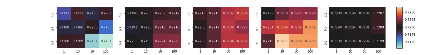
(a) ASSISTments2015

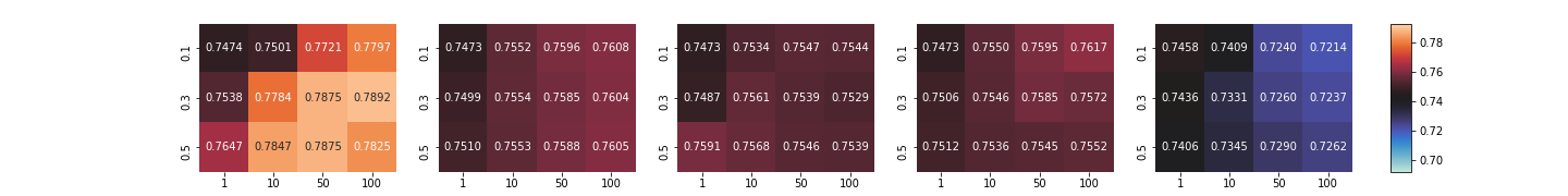
(b) ASSISTmentsChall

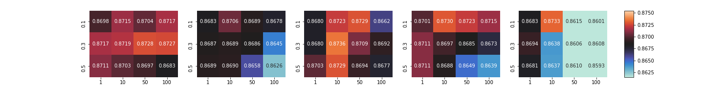
(c) STATICS2011

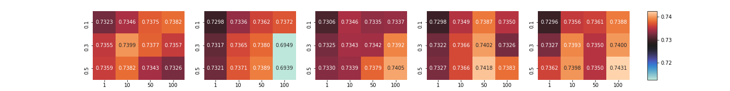
(d) EdNet-KT1

Figure 2: Test AUCs of the DKT model for each augmentation and corresponding regularization with different augmentation probabilities ($\alpha_{\mathrm{aug}})$) and regularization loss weights ($\lambda_{\mathrm{reg}-\mathrm{aug}}$). The hyperparameters are searched over $\alpha_{\mathrm{aug}}\in\{0.1,0.3,0.5\}$ and $\lambda_{\mathrm{reg}-\mathrm{aug}}\in\{1,10,50,100\}$. For each dataset, each column represents results with replacement, correct insertion, incorrect insertion, correct deletion, and incorrect deletion, from left to right. We set $\lambda_{\mathrm{aug}}=1$ for all cases. We use question-random replacement for ASSISTments2015 dataset.