Phase diagram of the three-band d-p model based on the optimization variational Monte Carlo method

Abstract

The phase diagram of cuprate high-temperature superconductors is investigated on the basis of the three-band d-p model. We use the optimization variational Monte Carlo method, where improved many-body wave functions have been proposed to make the ground-state wave function more precise. We investigate the stability of antiferromagnetic state by changing the band parameters such as the hole number, level difference $\Delta_{dp}$ between $d$ and $p$ electrons and transfer integrals. We show that the antiferromagnetic correlation weakens when $\Delta_{dp}$ decreases and the pure $d$-wave superconducting phase may exist in this region. We present phase diagrams including antiferromagnetic and superconducting regions by varying the band parameters. The phase diagram obtained by changing the doping rate $x$ contains antiferromagnetic, superconducting and also phase-separated phases. We propose that high-temperature superconductivity will occur near the antiferromagnetic boundary in the space of band parameters.

1 Introduction

The physics of high-temperature superconductivity has been studied from the viewpoint of strongly correlated electron systems since its discovery[1]. This is because cuprate parent materials are Mott insulators and the Cooper pairs have the d-wave symmetry. The fundamental model of cuprate high-temperature superconductors is the electronic model for the CuO₂ plane including copper and oxygen atoms. This model is called the d-p model (or three-band Hubbard model)[2, 3, 4, 5, 6, 7, 8, 9, 10, 11, 12, 13, 14, 15, 16, 17, 18]. It is certain that the electron correlation plays an important role in the d-p model since the on-site Coulomb interaction $U_{d}$ between d electrons is large. This makes it a difficult task to understand the phase diagram of the d-p model. Because $U_{d}$ is the large-energy scale interaction, new phenomena including high-temperature superconductivity can be expected. Simplified models such as the two-dimensional single-band Hubbard model[19, 20, 21, 22, 23, 24, 25, 26, 27, 28, 29, 30, 31, 32, 33, 34, 35, 36, 37, 38, 39, 40] or ladder model[41, 42, 43, 44, 45, 46] have been studied to investigate whether the attractive interaction is induced from the on-site Coulomb interaction.

We employ the optimization variational Monte Carlo method to investigate electronic properties of the three-band d-p model. In this method we calculate the expectation values of several physical properties numerically using a Monte Carlo algorithm[49, 47, 48]. In order to control the strong electron correlation, we use the Gutzwiller function and wave functions that are improved by multiplying an initial wave function by $\exp(-K)$-type operators[36, 49], where $K$ is a correlation operator with variational parameters. In this paper, $K$ stands for the non-interacting part of the Hamiltonian. In the single-band Hubbard model, the ground-state energy is lowered greatly and becomes lower than that obtained by other wave functions[36].

The single-band Hubbard model is the fundamental model and was used to understand the metal-insulator transition[50] and magnetic properties[51]. It has been shown from numerical studies based on improved wave functions that the superconducting phase exists in the single-band two-dimensional (2D) Hubbard model[31, 36, 37, 52, 53]. We regard the multi-band model as a more realistic model of high-temperature superconductors.

In this paper we investigate the stability of antiferromagnetically ordered state in the two-dimensional d-p model. The phase diagram is determined as a result of the competition between antiferromagnetic (AF) and superconducting (SC) pair correlations. The AF region decreases as the level difference $\epsilon_{p}-\epsilon_{d}$ decreases and thus the pure d-wave pairing phase may exist when $\epsilon_{p}-\epsilon_{d}$ is small. There is a phase separation (PS) in the low-doping region as in the two-dimensional Hubbard model[54, 55, 56, 57, 58]. We show the phase diagram as a function of the doping rate to show AF, SC and PS regions in the d-p model. We think that high-temperature superconductivity occurs in the crossover region near the boundary of AF phase[36, 37]. In the single-band Hubbard model, the crossover takes place as the on-site Coulomb interaction $U$ increases (or decreases). In the three-band d-p model, there are several parameters that can control AF correlation and would induce crossovers where AF or charge fluctuations grow larger.

2 Hamiltonian

We consider the three-band d-p model in this paper. The Hamiltonian is written as

$$H =\epsilon_{d}\sum_{i\sigma}d_{i\sigma}^{{\dagger}}d_{i\sigma}+\epsilon_{p}\sum_{i\sigma}(p_{i+\hat{x}/2\sigma}^{{\dagger}}p_{i+\hat{x}/2\sigma}$$

$$+p_{i+\hat{y}/2\sigma}^{{\dagger}}p_{i+\hat{y}/2\sigma})$$

$$+t_{dp}\sum_{i\sigma}[d_{i\sigma}^{{\dagger}}(p_{i+\hat{x}/2\sigma}+p_{i+\hat{y}/2\sigma}-p_{i-\hat{x}/2\sigma}-p_{i-\hat{y}/2\sigma})$$

$$+{\rm h.c.}]$$

$$+t_{pp}\sum_{i\sigma}[p_{i+\hat{y}/2\sigma}^{{\dagger}}p_{i+\hat{x}/2\sigma}-p_{i+\hat{y}/2\sigma}^{{\dagger}}p_{i-\hat{x}/2\sigma}$$

$$-p_{i-\hat{y}/2\sigma}^{{\dagger}}p_{i+\hat{x}/2\sigma}+p_{i-\hat{y}/2\sigma}^{{\dagger}}p_{i-\hat{x}/2\sigma}+{\rm h.c.}]$$

$$+t_{d}^{\prime}\sum_{\langle\langle ij\rangle\rangle\sigma}(d_{i\sigma}^{{\dagger}}d_{j\sigma}+{\rm h.c.})+U_{d}\sum_{i}d_{i\uparrow}^{{\dagger}}d_{i\uparrow}d_{i\downarrow}^{{\dagger}}d_{i\downarrow}.$$ (1)

$d_{i\sigma}$ and $d^{{\dagger}}_{i\sigma}$ represent the operators for the $d$ hole, and $p_{i\pm\hat{x}/2\sigma}$ and $p^{{\dagger}}_{i\pm\hat{x}/2\sigma}$ denote the operators for the $p$ holes at the site $R_{i\pm\hat{x}/2}$, and in a similar way $p_{i\pm\hat{y}/2\sigma}$ and $p^{{\dagger}}_{i\pm\hat{y}/2\sigma}$ are defined. $t_{dp}$ and $t_{pp}$ represent the transfer integrals between adjacent Cu and O orbitals and that between nearest neighbor p orbitals, respectively. $t_{d}^{\prime}$ was introduced to reproduce the Fermi surface[59] for cuprate superconductors. $U_{d}$ denotes the on-site Coulomb repulsion and $U_{p}$ is that between $p$ holes. In general, $U_{p}$ is smaller than $U_{d}$[60, 61, 62, 63, 64].

The values of band parameters have been estimated in the literature. For example, $U_{d}=10.5$, $U_{p}=4.0$ and $U_{dp}=1.2$ in eV[61] where $U_{dp}$ is the nearest-neighbor Coulomb interaction between holes on adjacent Cu and O orbitals. We neglect $U_{dp}$ because $U_{dp}$ is small compared to $U_{d}$. The level difference between $d$ and $p$ holes is denoted as $\Delta_{dp}=\epsilon_{p}-\epsilon_{d}$. $N$ stands for the number of sites and the total number of atoms is given by $N_{a}=3N$. The energy measured in units of $t_{dp}$ in this paper. We use the hole picture and we consider the case where $\Delta_{dp}\geq 0$ in this paper.

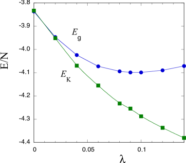
Figure 1: Ground-state energy $E_{g}$ and the kinetic energy $E_{K}=\langle K\rangle$ as a function of $\lambda$ on an $8\times 8$ lattice with 76 holes. The band parameters are $\epsilon_{p}-\epsilon_{d}=2t_{dp}$, $t_{pp}=0.4$, $t_{d}^{\prime}=-0.2$, $U_{d}=10$ and $U_{p}=0$ where the energy unit is $t_{dp}$.

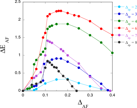
Figure 2: Antiferromagnetic condensation energy for $\psi_{\lambda}$ as a function of the AF gap parameter $\Delta_{AF}$ for several values of the level difference $\Delta_{dp}\equiv\epsilon_{p}-\epsilon_{d}$. We carried out calculations on an $8\times 8$ lattice (192 atoms) with 76 holes (where the doping rate $x$ is $x=0.1875$). We set $t_{pp}=0.4$, $t_{d}^{\prime}=0$ and $U_{d}=10$ in units of $t_{dp}$.

3 Improved wave functions with electron correlation

The wave function is given as

$$\psi_{\lambda}=\exp(-\lambda K)\psi_{G},$$ (2)

where $K$ denotes the non-interacting part of the Hamiltonian: $K=H$ with $U_{d}=0$. $\lambda$ is a real variational parameter. $\psi_{G}$ is given as $\psi_{G}=P_{G}\psi_{0}$ , with $P_{G}=\prod_{i}[1-(1-g)n_{di\uparrow}n_{di\downarrow}]$ where $g$ takes the value in the range $0\leq g\leq 1$. This is the wave function which is improved from the Gutzwiller function[36, 49, 65, 53, 66, 67, 68, 69, 37] generalized to the three-band model[70] by multiplying by an exponential factor. $\psi_{0}$ is a one-particle state with variational parameters $\tilde{t}_{dp}$, $\tilde{t}_{pp}$, $\tilde{t}^{\prime}_{d}$, $\tilde{\epsilon}_{p}-\tilde{\epsilon}_{d}$[70]: $\psi_{0}=\psi_{0}(\tilde{t}_{dp},\tilde{t}_{pp},\tilde{t}^{\prime}_{d},\tilde{\epsilon}_{p}-\tilde{\epsilon}_{d})$. $\psi_{0}$ is obtained as the eigenstate of the non-interacting Hamiltonian with these variational parameters. We set $\tilde{t}_{dp}=t_{dp}$ and the energy is measured in units of $t_{dp}$. $K$ also contains variational parameters: $K=K(\tilde{t}_{pp},\tilde{t}^{\prime}_{d},\tilde{\epsilon}_{p}-\tilde{\epsilon}_{d})$. The expectation values are calculated by using the variational Monte Carlo method.

We here give a discussion on the role $K$ in the wave function. The operator $e^{-\lambda K}$ controls the weights of excitation modes in the Gutzwiller function. $e^{-\lambda K}$ suppresses high-energy excitations for which the eigenvalues of $K$ are large and thus $e^{-\lambda k}$ becomes small. This indicates that $e^{-\lambda K}$ plays a role of projection that projects out low lying excitation modes from the wave function. This appears in the behavior of the momentum distribution function $n_{{\bf k}\sigma}\equiv\langle c_{{\bf k}\sigma}^{{\dagger}}c_{{\bf k}\sigma}\rangle$. In fact, $n_{{\bf k}\sigma}$ evaluated by the Gutzwiller function shows an unphysical behavior, that is, $n_{{\bf k}\sigma}$ at ${{\bf k}}$ near the Fermi surface is often larger than that at the bottom of the band[71]. This shortcoming is remedied by the improved wave function[59].

We show the energy-expectation value as a function of $\lambda$ in Fig. 1 where calculations were performed on the system of $8\times 8$ lattice with 76 holes. $E_{K}$ denotes the expectation value $E_{K}=\langle K\rangle$. The parameters are $\Delta_{dp}=\epsilon_{p}-\epsilon_{d}=2$, $t_{pp}=0.4$, $t_{d}^{\prime}=-0.2$ and $U_{d}=10$ in units of $t_{dp}$. The lowering of the total energy originates from the kinetic-energy gain as $\lambda$ is increased. The total energy given by the sum of the kinetic energy and the potential energy has a minimum at finite value of $\lambda$. Since the Coulomb potential energy increases as $\lambda$ increases, the total energy is determined by the balance between the kinetic energy and the Coulomb energy.

The correlated BCS wave function is written as

$$\psi_{\lambda-BCS}==\exp(-\lambda K)P_{G}\prod_{\bf k}(u_{\bf k}\beta_{\bf k}^{{\dagger}}+v_{\bf k}\alpha_{\bf k}^{{\dagger}})|\tilde{0}\rangle,$$ (3)

where the particle-hole transformation for down-spin holes[36, 53] has been performed: $\beta_{\bf k}^{{\dagger}}=\alpha_{-{\bf k}\downarrow}$ and $\alpha_{\bf k}^{{\dagger}}=\alpha_{{\bf k}\uparrow}^{{\dagger}}$. $|\tilde{0}\rangle$ denotes the vacuum for newly defined $\alpha$ and $\beta$ particles satisfying $\alpha_{\bf k}|\tilde{0}\rangle=\beta_{\bf k}|\tilde{0}\rangle=0$. The BCS parameter is given by the conventional form $v_{\bf k}/u_{\bf k}=\Delta_{\bf k}/(\xi_{\bf k}+\sqrt{\xi_{\bf k}^{2}+\Delta_{\bf k}^{2}})$, where $\xi_{\bf k}$ is the dispersion relation of the lowest band we assume the d-wave symmetry $\Delta_{\bf k}=\Delta(\cos k_{x}-\cos k_{y})$. $\Delta=\Delta_{sc}$ is a variational parameter and the optimized value $\Delta_{sc}$ is regarded as the superconducting gap. In this representation, the electron pair operator $\alpha_{{\bf k}\uparrow}^{{\dagger}}\alpha_{{\bf k}\downarrow}^{{\dagger}}$ is transformed to the hybridization form $\alpha_{{\bf k}}^{{\dagger}}\beta_{{\bf k}}$. The chemical potential is used to adjust the expectation value of the total electron number.

4 Antiferromagnetic state and the level difference

The antiferromagnetic wave function is formulated by introducing the AF order parameter $\Delta_{AF}$ in the initial wave function $\psi_{0}(\Delta_{AF})$:

$$\psi_{\lambda}=\exp(-\lambda K)P_{G}\psi_{0}(\Delta_{AF}).$$ (4)

The level difference $\Delta_{dp}=\epsilon_{p}-\epsilon_{d}$ plays an important role in determining the stability of the AF state. We show the AF condensation energy $\Delta E_{AF}$ as a function of the AF order parameter $\Delta_{AF}$ for several values of the level difference between d and p electrons in Fig. 2. We carried out calculations on a system of $8\times 8$ lattice with 192 atoms including copper and oxygen atoms. $\Delta E_{AF}$ has a maximum when the level difference $\Delta_{dp}$ is about half of $U_{d}$, namely, near the ’symmetric case’ with $\Delta_{dp}=U_{d}/2$. In Fig. 2, we set the parameters as $t_{pp}=0.4$, $t_{d}^{\prime}=0$ and $U_{d}=10$ in units of $t_{dp}$, and the doping rate is $x=0.1875$. We show $\Delta E_{AF}/N$ as a function of the level difference $\Delta_{dp}$ for $t_{d}^{\prime}=0$ and $-0.2$ in Fig. 3. The AF order parameter $\Delta_{AF}$ at which $\Delta E_{AF}$ takes a maximum value is shown in Fig. 4 for each value of $\Delta_{dp}$. For $t_{d}^{\prime}=0$, $\Delta_{AF}$ vanishes when $\Delta_{dp}\simeq 1$. This indicates that we may have a superconducting phase when the d-hole level is near the p-hole level. The results in Figs. 3 and 4 also show that $t_{d}^{\prime}$ suppresses the magnetic instability.

We show $\Delta E_{AF}/N$ as a function of $\Delta_{dp}$ when the doping rate is $x=0.125$ in Fig. 5. The Fig. 5 shows that $\Delta E_{AF}$ has also a maximum for $\Delta_{dp}\sim U_{d}/2$ and AF correlation survives even up to the region of small $\Delta_{dp}\sim 1$ for small $x$.

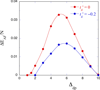
Figure 3: Antiferromagnetic condensation energy for $\psi_{\lambda}$ as function of the level difference $\Delta_{dp}=\epsilon_{p}-\epsilon_{d}$ on an $8\times 8$ lattice with 76 holes. We used $t_{pp}=0.4$ and $U_{d}=10$ in units of $t_{dp}$.

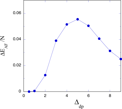
Figure 4: Antiferromagnetic condensation energy for $\psi_{\lambda}$ as function of the level difference $\Delta_{dp}$ on an $8\times 8$ lattice with 72 holes ($x=0.125$). We set $t_{pp}=0.4$, $t_{d}^{\prime}=0$ and $U_{d}=10$.

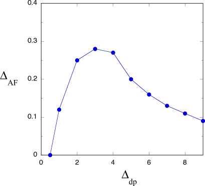
Figure 5: Antiferromagnetic order parameter for $\psi_{\lambda}$ as function of the level difference $\Delta_{dp}$ on an $8\times 8$ lattice with 72 holes. The parameers are the same as in Fig.5.

5 Superconducting state

First we examine the superconducting state by employing the BCS-Gutzwiller wave function $\psi_{G-BCS}=P_{N_{e}}P_{G}\psi_{BCS}$, where $\psi_{BCS}$ indicates the BCS wave function. $P_{N_{e}}$ is the number-projection operator that extracts only the states with a fixed total hole number. We show the SC condensation energy as a function of the SC order parameter $\Delta_{sc}$ in Fig.6 for several values of the level difference $\Delta_{dp}$. The result shows that the SC condensation energy increases as $\Delta_{dp}$ increases. Based on the BCS-Gutzwiller function, the large level difference is more favorable for superconductivity. We should, however, remember instability toward antiferromagnetic state when the level difference $\Delta_{dp}$ becomes large.

From the competition between AF and SC orderings, we expect that the pure $d$-wave SC state is stabilized when $\epsilon_{d}-\epsilon_{p}$ is near the boundary of the AF region. The AF and SC order parameters are shown as a function of $\Delta_{dp}$ in Fig. 7 for $x=0.1875$. We included the SC order parameter for the Gutzwiller function for reference when $\Delta_{dp}\geq 2t_{dp}$ although SC state is no longer stable in this region. This figure indicates that the SC state exists when the level difference is small and that high-temperature superconductivity will occur in the small $\Delta_{dp}$-region.

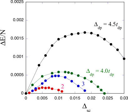
Figure 6: SC condensation energy for the BCS-Gutzwiller function as function of the superconducting gap parameter $\Delta_{sc}$ for several values of the level difference $\Delta_{dp}\equiv\epsilon_{p}-\epsilon_{d}$. The calculations were carried out on an $8\times 8$ lattice with $t_{pp}=0.4$, $t_{d}^{\prime}=0$ and $U_{d}=10$ in units of $t_{dp}$. The number of holes is 76 for $\Delta_{dp}=3$, 4 and 4.5 and 72 for $\Delta_{dp}=2$ (closed shell cases).

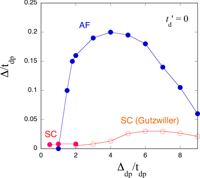
Figure 7: AF and SC order parameters for the $\psi_{\lambda}$ wave function as a function of the level difference $\Delta_{dp}$. The SC order parameter obtained by the Gutzwiller function is also shown by open circles for reference in the region $\Delta_{dp}\geq 2t_{dp}$. We set $x=0.1875$ and the band parameters are $t_{pp}=0.4$, $t_{d}^{\prime}=0$ and $U_{d}=10$.

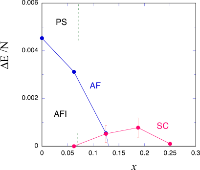
Figure 8: AF and SC condensation energies as a function of the hole doping rate $x$ for $\Delta_{dp}=1$ on a $8\times 8$ lattice with $t_{pp}=0.4$, $t_{d}^{\prime}=0$ and $U_{d}=10$ in units of $t_{dp}$. There is a phase-separated region when $x$ is small.

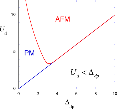
Figure 9: AF region in the plane of $U_{d}$ and the level difference $\Delta_{dp}$ for $x=0.1875$ on an $8\times 8$ lattice. We set $t_{pp}=0.4$ and $t_{d}^{\prime}=0$, and the energy is measured in units of $t_{dp}$.

6 Phase diagram and phase separation

Let us examine the possible phase diagram of cuprate superconductors based on the optimization variational Monte Carlo method. We exhibit the condensation energy as a function of the doping rate $x$ for $\Delta_{dp}=t_{dp}$ in Fig. 8. There is the AF region when $x$ is small and the SC region exists near the optimum region $x\sim 0.2$. We should mention that there is a phase-separated region in the low-doping region where $x<0.07$. This indicates the existence of AF insulator phase in the low doping region. This is similar to the phase diagram of the 2D Hubbard model. The phase separation (PS) is, however, dependent on the level difference $\Delta_{dp}$. As $\Delta_{dp}$ decreases, the phase-separated region decreases and vanishes when $\Delta_{dp}$ approaches zero. Thus the area of phase-separated region can be controlled by changing the band parameters.

We lastly show the phase diagram in the $U_{d}$-$\Delta_{dp}$ plane for $x=0.1875$ with $t_{pp}=0.4t_{dp}$ and $t_{d}^{\prime}=0$ in Fig. 9. There are a large AF region and paramagnetic(PM) phase in Fig. 9 where SC regions are not explicitly included. We expect that high-temperature superconductivity may be realized in the relatively small region near the boundary between AF and PM regions.

7 Summary

We have investigated the ground-state properties of the three-band d-p model on the basis of the optimization variational Monte Carlo method. The ground-state energy is lowered greatly by multiplying by the exponential operator $e^{-\lambda K}$ as in the 2D Hubbard model. In general, the antiferromagnetic correlation is suppressed as the wave function is improved.

In the d-p model the AF correlation is very much stronger than that in the single-band Hubbard model. It is thus important to control the strength of AF correlation by varying the interaction and band parameters. The level difference $\Delta_{dp}$ plays an important role in the study of the phase diagram of the d-p model. The pure $d$-wave superconducting phase exists when $\Delta_{dp}$ becomes small. In particular high-temperature superconductivity is expected near the AF boundary in the small $\Delta_{dp}$ region.

A phase-separated region exists in the d-p model as in the single-band 2D Hubbard model. In this region the ground state is an insulator with AF order and is dependent upon $\Delta_{dp}$. The PS region increases as $\Delta_{dp}$ increases and decreases and vice versa. The close relation between PS region and incommensurate phases have been examined[56, 57]. The PS instability may be related to an instability toward some charge order such as stripes.

The phase diagram in Fig. 9 is consistent with several experiments concerning the critical temperature $T_{c}$ of cuprate superconductors[72, 73]. There is a correlation between $T_{c}$ and the ratio of hole numbers $n_{p}/n_{d}$ where $n_{p}$ and $n_{d}$ denote the hole density of p and d holes, respectively[72]. There is the tendency that $T_{c}$ is higher for larger $n_{p}/n_{d}$, that is, $T_{c}$ increases with the decrease of $\epsilon_{p}-\epsilon_{d}$. This is consistent with our result that the pure d-wave pairing state exists when $\epsilon_{p}-\epsilon_{d}$ is small.

The increase of $T_{c}$ under pressure[73] is understood within the d-p model as follows. $\Delta_{dp}$ and $U_{d}$ would decrease by applying pressure. If the first electronic state is not in the optimum SC state near the AF boundary, $T_{c}$ will increase as $\Delta_{dp}$ decreases.

We neglected Cu-O Coulomb repulsion $U_{dp}$ in this paper. It has been pointed out that a small $U_{dp}$ can produce dramatic consequences on the charge stability[54, 74]. It is a future issue to examine the effect of $U_{dp}$. It is well known that the parent compounds of high-temperature cuprates are charge-transfer insulators. Based on the optimization variational Monte Carlo method, the critical value of $\Delta_{dp}$ for charge-transfer metal-insulator transition is about $2t_{dp}$[59]. In our calculations the favorable value of $\Delta_{dp}$ for superconductivity is a little bit smaller than this critical value because of competition between AF and SC correlations. This would indicate a possibility that the critical temperature $T_{c}$ can be increased by changing material parameters. We also mention that the inclusion of $U_{dp}$ or band parameter $t_{d}^{\prime}$ possibly may change the physical picture.

A part of computations was supported by the Supercomputer Center of the Institute for Solid State Physics, the University of Tokyo, and the Supercomputer system Yukawa-21 of the Yukawa Institute for Theoretical Physics, Kyoto University. This work was supported by a Grand-in-Aid for Scientific Research from the Ministry of Education, Culture, Sports, Science and Technology of Japan (Grant No. 17K05559).

References

- [1] J. G. Bednorz and K. A. Müller, Z. Phys. B 64, 189 (1986).
- [2] V. J. Emery, Phys. Rev. Lett. 58, 2794 (1987).
- [3] J. E. Hirsch, E. Y. Loh, D. J. Scalapino, and S. Tang, Phys. Rev. B 39, 243 (1989).
- [4] R. T. Scalettar, D. J. Scalapino, R. L. Sugar, and S. R. White, Phys. Rev. B 44, 770 (1991).
- [5] A. Oguri, T. Asahata, and S. Maekawa, Phys. Rev. B 49, 6880 (1994).
- [6] S. Koikegami and K. Yamada, J. Phys. Soc. Jpn. 69, 768 (2000).
- [7] T. Yanagisawa, S. Koike and K. Yamaji, Phys. Rev. B 64, 184509 (2001).
- [8] S. Koikegami and T. Yanagisawa, J. Phys. Soc. Jpn. 70, 3499 (2001).
- [9] T. Yanagisawa, S. Koike and K. Yamaji, Phys. Rev. B 67, 132408 (2003).
- [10] S. Koikegami and T. Yanagisawa, Phys. Rev. B 67, 134517 (2003).
- [11] S. Koikegami and T. Yanagisawa, J. Phys. Soc. Jpn. 75, 034715 (2006).
- [12] T. Yanagisawa, M. Miyazaki and K. Yamaji, J. Phys. Soc. Jpn. 78, 013706 (2009).
- [13] C. Weber, A. Lauchi, F. Mila and T. Giamarchi, Phys. Rev. Lett. 102, 017005 (2009).
- [14] B. Lau, M. Berciu and G. A. Sawatzky, Phys. Rev. Lett. 106, 036401 (2011).
- [15] C. Weber, T. Giamarchi and C. M. Varma, Phys. Rev. Lett. 112, 117001 (2014).
- [16] A. Avella, F. Mancini, F. Paolo and E. Plekhanov, Euro. Phys. J. B 86, 265 (2013).
- [17] H. Ebrahimnejad, G. A. Sawatzky and M. Berciu, J. Phys. Cond. Matter 28, 105603 (2016).
- [18] S. Tamura and H. Yokoyama, Phys. Procedia 81, 5 (2016).
- [19] J. Hubbard, Proc. R. Soc. London 276, 238 (1963).
- [20] J. Hubbard, Proc. R. Soc. London 281, 401 (1963).
- [21] M. C. Gutzwiller, Phys. Rev. Lett. 10, 159 (1963).
- [22] S. Zhang, J. Carlson and J. E. Gubernatis, Phys. Rev. B 55, 7464 (1997).
- [23] S. Zhang, J. Carlson and J. E. Gubernatis, Phys. Rev. Lett. 78, 4486 (1997).
- [24] Yanagisawa T and Shimoi Y 1996 Int. J. Mod. Phys. B 10 3383.
- [25] T. Nakanishi, K. Yamaji and T. Yanagisawa, J. Phys. Soc. Jpn. 66, 294 (1997).
- [26] K. Yamaji, T. Yanagisawa, T. Nakanishi and S. Koike, Physica C 304, 225 (1998).
- [27] K. Yamaji, T. Yanagisawa, M. Miyazaki and R. Kadono, J. Phys. Soc. Jpn. 80, 083702 (2011).
- [28] T. M. Hardy, P. Hague, J. H. Samson and A. S. Alexandrov, Phys. Rev. B 79, 212501 (2009).
- [29] N. Bulut, Adv. Phys. 51, 1587 (2002).
- [30] H. Yokoyama, Y. Tanaka, M. Ogata and H. Tsuchiura, J. Phys. Soc. Jpn. 73, 1119 (2004).
- [31] H. Yokoyama, M. Ogata and Y. Tanaka, J. Phys. Soc. Jpn. 75, 114706 (2006).
- [32] T. Aimi and M. Imada, J. Phys. Soc. Jpn. 76, 113708 (2007).
- [33] M. Miyazaki, T. Yanagisawa and K. Yamaji, J. Phys. Soc. Jpn. 73, 1643 (2004).
- [34] T. Yanagisawa, New J. Phys. 10, 023014 (2008).
- [35] T. Yanagisawa, New J. Phys. 15, 033012 (2013).
- [36] T. Yanagisawa, J. Phys. Soc. Jpn. 85, 114707 (2016).
- [37] T. Yanagisawa, J. Phys. Soc. Jpn. 88, 054702 (2019).
- [38] T. Yanagisawa, Condensed Matter 4, 57 (2019).
- [39] T. Yanagisawa, Phys. Lett. A 403, 127382 (2021).
- [40] T. Yanagisawa, Condensed Matter 6, 12 (2021).
- [41] R. M. Noack, S. R. White and D. J. Scalapino, EPL 30, 163 (1995).
- [42] R. M. Noack, N. Bulut, D. J. Scalapino and M. G. Zacher, Phys. Rev. B 56, 7162 (1997).
- [43] K. Yamaji, Y. Shimoi and T. Yanagisawa, Physica C 235, 2221 (1994).
- [44] S. Koike, K. Yamaji, and T. Yanagisawa, J. Phys. Soc. Jpn. 68, 1657 (1999).
- [45] T. Yanagisawa, Y. Shimoi and K. Yamaji, Phys. Rev. B 52, R3860 (1995).
- [46] T. Nakano, K. Kuroki and S. Onari, Phys. Rev. B 76, 014515 (2007).
- [47] R. Blankenbecler, D. J. Scalapino and R. L. Sugar, Phys. Rev. D 24, 2278 (1981).
- [48] T. Yanagisawa, Phys. Rev. B 75, 224503 (2007).
- [49] T. Yanagisawa, S. Koike and K. Yamaji, J. Phys. Soc. Jpn. 67, 3867 (1998).
- [50] N. F. Mott, Metal-Insulator Transitions (Taylor & Francis, London, 1974).
- [51] K. Yosida, Theory of Magnetism (Springer, Berlin, 1996).
- [52] T. Misawa and M. Imada, Phys. Rev. B90, 115137 (2014).
- [53] T. Yanagisawa, S. Koike and K. Yamaji, J. Phys. Soc. Jpn. 68, 3608 (1999).
- [54] N. Cancrini, S. Caprara, C. Castellani, C. Di Castro, M. Grilli and R. Raimondi, EPL 14, 597 (1991).
- [55] S. Caprara, C. Di Castro and M. Grilli, Phys. Rev. B 51, 9286 (1995).
- [56] J. Lorenzana and G. Seibold, Phys. Rev. Lett. 89, 136401 (2002).
- [57] F. Günther, G. Seibold and J. Lorenzana, Phys. Rev. Lett. 98, 176404 (2007).
- [58] L. F. Tocchio, F. Becca and S. Sorella, Phys. Rev. B 94, 195126 (2016).
- [59] T. Yanagisawa and M. Miyazaki, EPL 107, 27004 (2014).
- [60] C. Weber, K. Haule, and G. Kotliar, Phys. Rev. B 78, 134519 (2008).
- [61] M. S. Hybertsen, M. Schluter, and N. E. Christensen, Phys. Rev. B 39, 9028 (1989).
- [62] H. Eskes, G. A. Sawatzky, and L. F. Feiner, Physica C 160, 424 (1989).
- [63] A. K. McMahan, J. F. Annett, and R. M. Martin, Phys. Rev. B 42, 6268 (1990).
- [64] H. Eskes and G. Sawatzky, Phys. Rev. B 43, 119 (1991).
- [65] H. Otsuka, J. Phys. Soc. Jpn. 61, 1645 (1992).
- [66] D. Eichenberger and D. Baeriswyl, Phys. Rev. B 76, 180504 (2007).
- [67] D. Baeriswyl, D. Eichenberger and M. Menteshashvii, J. Phys. 11, 075010 (2009).
- [68] D. Baeriswyl, J. Supercond. Novel Magn. 24, 1157 (2011).
- [69] D. Baeriswyl, Phys. Rev. B 99, 235152 (2019).
- [70] T. Yanagisawa, J. Phys. Conf. Ser. 1293, 012027 (2019).
- [71] H. Yokoyama and H. Shiba, J. Phys. Soc. Jpn. 56, 1490 (1986).
- [72] G.-Q. Zheng, Y. Kitaoka, K. Ishida and K. Asayama, J. Phys. Soc. Jpn. 64, 2524 (1995).
- [73] N. Takeshita, A. Yamamoto, A, Iyo and H. Eisaki, J. Phys. Soc. Jpn. 82, 023711 (2013).
- [74] R. Raimondi and C. Castellani, Phys. Rev. B 48, 11453 (R) (1993).