State-Operator Correspondence in Celestial Conformal Field Theory

Erin Crawley^∗, Noah Miller^∗, Sruthi A. Narayanan^∗, and Andrew Strominger^∗

^∗Center for the Fundamental Laws of Nature, Harvard University,
Cambridge, MA 02138, USA

The bulk-to-boundary dictionary for 4D celestial holography is given a new entry defining 2D boundary states living on oriented circles on the celestial sphere. The states are constructed using the 2D CFT state-operator correspondence from operator insertions corresponding to either incoming or outgoing particles which cross the celestial sphere inside the circle. The BPZ construction is applied to give an inner product on such states whose associated bulk adjoints are shown to involve a shadow transform. Scattering amplitudes are then given by BPZ inner products between states living on the same circle but with opposite orientations. 2D boundary states are found to encode the same information as their 4D bulk counterparts, but organized in a radically different manner.

1 Introduction

The symmetries of every asymptotically flat 4D bulk quantum theory of gravity include the local conformal group acting in antipodal unison on the past and future celestial spheres at null infinity [1, 2]. This implies that the $\cal S$-matrix can be holographically recast as boundary correlators of a 2D “celestial conformal field theory” (CCFT) living on the celestial sphere [3, 4, 5, 6, 7, 8, 9]. The operators inserted in the correlator can correspond to both incoming and outgoing particles crossing the celestial sphere. The so-defined CCFT correlators enjoy some, but not all, properties of those in a garden-variety 2D CFT. It is an important open challenge to find an intrinsic construction of any CCFT (i.e. other than as a transformation of a bulk theory) starting with a microscopic theory such as string theory. However, it is implausible that such a construction will be possible for the real world any time soon as it would amount to a complete knowledge of all the laws of physics. Nevertheless, many properties of CCFT can be deduced from their rich symmetry properties and logical self-consistency conditions.

In this paper we deduce entries in the celestial holographic bulk-to-boundary dictionary concerning the relation between the 4D bulk and 2D boundary Hilbert spaces, inner products and scattering problems. In the familiar case of AdS/CFT holography [10], there is a very simple correspondence between bulk and boundary states: they are different descriptions of the same thing. Such a simple relation cannot possibly hold in celestial holography as the boundary is Euclidean while the bulk is Lorentzian. A pair of 2D states can be defined by dividing the celestial sphere into northern and southern hemispheres. The northern and southern operator insertions - both incoming and outgoing - then define “northern” and “southern” states on the celestial sphere. The inner product of a northern and southern 2D state is then a scattering amplitude. Hence, boundary states exist along with bulk states but they organize the information about the theory in a fascinating and very different manner.

To construct a 2D inner product it is insightful to first understand the 4D bulk product from which it can be derived. The Klein-Gordon inner product provides a natural positive-definite norm on the bulk Hilbert space. However, it is unnatural from the boundary perspective both because it gives delta functions on the celestial sphere for conformal primaries [7, 9] and because the conformal generators have non-standard adjoint properties [11, 12]. A second conserved inner product is given by the classic Belavin, Polyakov and Zamolodchikov (BPZ) construction [13], which starts with a CFT₂ two-point function with operators inserted at opposite poles. This construction applies directly to CCFT in which the CFT₂ two-point function is given by the two-particle $\cal S$-matrix written in the conformal basis. The resulting inner product is indefinite, which is to be expected since states in the CCFT can have negative or complex conformal weights. We show that from the bulk perspective the BPZ adjoint of a 2D conformal primary state thereby involves a shadow transform [14, 15] replacing the standard Klein-Gordon complex conjugation. Shadowing one of the primary fields in the two-point function transforms the delta function to the more familiar CFT₂ power law. Shadows have been ubiquitous in discussions of CCFT, indeed in [16] the scattering of shadow states was recently derived and found to have elegant factorization properties.

This paper is organized as follows. Section 2 begins with a review of conserved 4D bulk inner products, including the origin of delta functions in the Klein-Gordon inner product of conformal primaries. The conserved bulk shadow product, in which the shadow replaces complex conjugation, is introduced and computed for conformal primaries. It is shown to have both the familiar boundary power-law behavior dictated by conformal invariance and the familiar adjoint relations for conformal generators. In section 3 we describe how conformal invariance allows us to associate a state living on the circle surrounding every operator insertion. These states are defined explicitly using the operators appearing in the mode expansions of conformal primaries. We then construct the BPZ inner product of these states from the two-point function, and show that for CCFT the adjoint state involves a shadow transform. Viewed as a bulk inner product on single-particle states, we recover the shadow product of section 2. We close in section 4 with a discussion of the holographic relation, in the multi-particle context, between the 2D boundary Hilbert space and the 4D bulk Hilbert space. We also relate the boundary scattering problem, which concerns a map between “northern” and “southern” states on the respective hemispheres of the celestial sphere, with the bulk scattering problem which concerns a map from past to future null infinity.

Throughout this paper we use the terms “inner product” and “Hilbert space” to include indefinite inner products and Hilbert spaces.

2 Bulk inner products

In order to define an inner product on the 2D boundary, we must first discuss the 4D bulk products to which they are related. In this section we discuss two standard products on the 4D bulk space, the Klein-Gordon and symplectic, as well as a modification of them involving the shadow transform which will prove to be useful in the subsequent discussion about 2D CCFT inner products.

2.1 Symplectic and Klein-Gordon products

Consider 4D Minkowski space with the standard metric

$$ds^{2}=\eta_{\mu\nu}dX^{\mu}dX^{\nu}=-\left(dX^{0}\right)^{2}+\left(dX^{1}\right)^{2}+\left(dX^{2}\right)^{2}+\left(dX^{3}\right)^{2},$$ (2.1)

and let $\Phi_{1,2}$ denote any two solutions of the scalar wave equation. From these one can construct the symplectic current

$$J_{\mu}(\Phi_{1},\Phi_{2})=\Phi_{1}\overleftrightarrow{\partial}_{\mu}\Phi_{2}\equiv\Phi_{1}(\partial_{\mu}\Phi_{2})-(\partial_{\mu}\Phi_{1})\Phi_{2},$$ (2.2)

which is conserved:

$$\partial^{\mu}J_{\mu}=0.$$ (2.3)

The symplectic product of two wavefunctions is accordingly defined as

$$(\Phi_{1},\Phi_{2})_{\rm sym}=\int_{\Sigma_{3}}d^{3}\Sigma^{\mu}J_{\mu}(\Phi_{1},\Phi_{2}).$$ (2.4)

This product is conserved in the sense that it is independent of the choice of complete spacelike slice $\Sigma_{3}$. Since $J_{\mu}$ is conserved for any pair of solutions, there are many possible conserved scalar products, a freedom which is exploited below. For example, the usual Klein-Gordon product is obtained from the symplectic product as

$$(\Phi_{1},\Phi_{2})_{\rm{KG}}=-i\int_{\Sigma_{3}}d^{3}\Sigma^{\mu}J_{\mu}(\Phi_{1},\Phi_{2}^{*})=-i(\Phi_{1},\Phi_{2}^{\ast})_{\rm{sym}},$$ (2.5)

and is also conserved. One can use the Klein-Gordon product to construct a positive definite 4D Hilbert space in the usual way. Similar inner products can be constructed from symplectic structures [17] for arbitrary integer spin $J$. The treatment of half-integer spin $J$ requires an inner product like the Dirac inner product considered in [18, 19, 20].

2.2 Lorentz generators and their adjoints

We will be interested in the action of the Lorentz group on these wavefunctions which is infinitesimally generated by the Lie action of the six vector fields

$$\xi_{1} = -\frac{1}{2}\left[(X^{1}+iX^{2})(\partial_{0}+\partial_{3})+(X^{0}-X^{3})(\partial_{1}+i\partial_{2})\right]$$ (2.6)

$$\xi_{0} = -\frac{1}{2}\left[X^{3}\partial_{0}-iX^{2}\partial_{1}+iX^{1}\partial_{2}+X^{0}\partial_{3}\right]$$ (2.7)

$$\xi_{-1} = \frac{1}{2}\left[(X^{1}-iX^{2})(\partial_{0}-\partial_{3})+(X^{0}+X^{3})(\partial_{1}-i\partial_{2})\right]$$ (2.8)

$$\bar{\xi}_{1} = -\frac{1}{2}\left[(X^{1}-iX^{2})(\partial_{0}+\partial_{3})+(X^{0}-X^{3})(\partial_{1}-i\partial_{2})\right]$$ (2.9)

$$\bar{\xi}_{0} = -\frac{1}{2}\left[X^{3}\partial_{0}+iX^{2}\partial_{1}-iX^{1}\partial_{2}+X^{0}\partial_{3}\right]$$ (2.10)

$$\bar{\xi}_{-1} = \frac{1}{2}\left[(X^{1}+iX^{2})(\partial_{0}-\partial_{3})+(X^{0}+X^{3})(\partial_{1}+i\partial_{2})\right]$$ (2.11)

obeying $\bar{\xi}_{n}=(\xi_{n})^{\ast}$. Denoting their Lie action by $L_{n}=-\mathcal{L}_{\xi_{n}},\bar{L}_{n}=-\bar{\mathcal{L}}_{\bar{\xi}_{n}},$ one finds

$$[L_{m},L_{n}]=(m-n)L_{m+n},~{}~{}~{}~{}[\bar{L}_{m},\bar{L}_{n}]=(m-n)\bar{L}_{m+n}.$$ (2.12)

It is straightforward to verify that [11]

$$(\Phi_{1},L_{n}\Phi_{2})_{\rm{KG}}=-(\bar{L}_{n}\Phi_{1},\Phi_{2})_{\rm{KG}}$$ (2.13)

for $\Phi_{1,2}$, which decay sufficiently rapidly at infinity. Hence with respect to this scalar product the adjoint is

$$L_{n}^{\dagger}=-\bar{L}_{n}.$$ (2.14)

Note that this is not the standard adjoint relation $L_{n}^{\dagger}=L_{-n}$ which one would expect in CFT₂. However, when we define our celestial inner product, we will indeed recover the more standard adjoint equation in that setting.

2.3 Conformal primary wavefunctions

Bulk 4D $\mathcal{S}$-matrix elements in momentum space can be recast as “celestial amplitudes” that transform like 2D conformal correlators by way of a Mellin transform. Celestial amplitudes are constructed by scattering states which are SL$(2,\mathbb{C})$ primary wavefunctions rather than momentum space plane waves [7, 9]. These states $\phi_{\pm,\Delta,J}^{\mu_{1}\ldots\mu_{s}}\left(X^{\mu};w,\bar{w}\right)$, referred to as conformal primary wavefunctions, are labelled by an arbitrary complex conformal dimension $\Delta$, spin $J$, ingoing/outgoing subscript $\pm$ and a point $(w,\bar{w})$ where they cross the celestial sphere. In what follows we label them by their conformal weights $(h,\bar{h})$, related in the usual way by

$$(h,\bar{h})=\left(\frac{1}{2}(\Delta+J),\frac{1}{2}(\Delta-J)\right).$$ (2.15)

Under Lorentz and conformal transformations primary wavefunctions satisfy

$$\Lambda_{\nu_{1}}^{\mu_{1}}\ldots\Lambda_{\nu_{s}}^{\mu_{s}}\phi_{\pm,h,\bar{h}}^{\nu_{1}\ldots\nu_{s}}\left((\Lambda^{-1})^{\mu}_{\nu}X^{\nu};w,\bar{w}\right)=(cw+d)^{-2h}(\bar{c}\bar{w}+\bar{d})^{-2\bar{h}}\phi_{\pm,h,\bar{h}}^{\mu_{1}\ldots\mu_{s}}\left(X^{\mu};\frac{aw+b}{cw+d},\frac{\bar{a}\bar{w}+\bar{b}}{\bar{c}\bar{w}+\bar{d}}\right).$$ (2.16)

The infinitesimal version of this equation is

$$L_{n}\phi_{\pm,h,\bar{h}}^{\mu_{1}\ldots\mu_{s}}(X^{\mu},w,\bar{w})=(w^{n+1}\partial_{w}+h(n+1)w^{n})\phi^{\mu_{1}\ldots\mu_{s}}_{\pm,h,\bar{h}}(X^{\mu},w,\bar{w}),$$ (2.17)

and likewise for $\bar{L}_{n}$. The continuum of modes obtained by Mellin transforms on the unitary principal series $\Delta=1+i\lambda$ for $\lambda\in\mathbb{R}$ are of special interest [9] because they comprise a complete basis of solutions for normalizable radiative wave packets. The symplectic product between two integer spin conformal primary wavefunctions on the unitary principal series is

$$\left(\phi_{\pm,h_{1},\bar{h}_{1}}^{\mu_{1}\ldots\mu_{s}}(X^{\mu};w_{1},\bar{w}_{1}),\phi_{\mp,h_{2},\bar{h}_{2}}^{\nu_{1}\ldots\nu_{s}}(X^{\mu};w_{2},\bar{w}_{2})\right)_{\rm sym}=\mathcal{C}^{\pm}_{J_{1}}(\lambda_{1})\delta_{J_{1}-J_{2}}\delta(\lambda_{1}+\lambda_{2})\delta^{(2)}(w_{1}-w_{2}),$$ (2.18)

where $\mathcal{C}^{\pm}_{J_{1}}(\lambda_{1})$ is a normalization that can be found in [9].

As an explicit example, for the case of massless scalars, conformal primary wavefunctions take the form

$$\varphi_{\pm,h,\bar{h}}(X^{\mu};\vec{w})=\frac{(\mp i)^{\Delta}\Gamma(\Delta)}{(-q(\vec{w})\cdot X\mp i\epsilon)^{\Delta}},$$ (2.19)

where $q(\vec{w})=(1+w\bar{w},w+\bar{w},i(\bar{w}-w),1-w\bar{w})$ is a null vector which points to $w=\frac{q^{1}+iq^{2}}{q^{0}+q^{3}}$ on the celestial sphere. The symplectic product is

$$\left(\varphi_{\pm,h_{1},\bar{h}_{1}}(X^{\mu};w_{1},\bar{w}_{1}),\varphi_{\mp,h_{2},\bar{h}_{2}}(X^{\mu};w_{2},\bar{w}_{2})\right)_{\rm sym}=\pm 8i\pi^{4}\delta(\lambda_{1}+\lambda_{2})\delta^{(2)}(w_{1}-w_{2}),$$ (2.20)

so we see that the normalization is $\mathcal{C}^{\pm}_{0}(\lambda_{1})=\pm 8i\pi^{4}$. Likewise the Klein-Gordon product is

$$(\varphi_{\pm,h_{1},\bar{h}_{1}}(X^{\mu};w_{1},\bar{w}_{1}),\varphi_{\pm,h_{2},\bar{h}_{2}}(X^{\mu};w_{2},\bar{w}_{2}))_{\rm sym}=\pm 8\pi^{4}\delta(\lambda_{1}-\lambda_{2})\delta^{(2)}(w_{1}-w_{2}).$$ (2.21)

2.4 Shadow product

One of the goals of rewriting 4D scattering amplitudes in a conformal basis is to apply the powerful techniques of CFT₂ to analyze and constrain them. For a free theory, as we consider in this work, the momentum-space $\mathcal{S}$-matrix elements for one incoming and one outgoing particle are given by the Klein-Gordon product of plane waves. The Mellin transform of these $\mathcal{S}$-matrix elements are bulk products of conformal primary wavefunctions and can be identified with a CFT₂ two-point function. However, while the result (2.18) is certainly fully conformally invariant, one expects to see a factor $(z-w)^{-2h}(\bar{z}-\bar{w})^{-2\bar{h}}$ in a CFT₂ two-point function rather than the delta function $\delta^{(2)}(z-w)$. Moreover, the adjoint relation $L_{n}^{\dagger}=-\bar{L}_{n}$ derived from the Klein-Gordon inner product is not the one usually encountered in CFT₂. Rather we expect the conformal generators to obey $L_{n}^{\dagger}=L_{-n}$.

Since both of these unfamiliar properties derive from the choice of inner product, we here consider modified inner products. If $\mathcal{M}$ is any map on the space of solutions, a new conserved product can be constructed from $J_{\mu}(\mathcal{M}\Phi_{1},\Phi_{2})$. Such modified products have been considered in many contexts, including holographic ones similar to the current case in [23, 11, 12, 24]. A useful choice of $\mathcal{M}$ is provided by the 2D shadow transform $\mathcal{S}$ [14, 15], which takes $J\to-J$ and $\Delta\to 2-\Delta$ thereby taking a field of conformal weight $(h,\bar{h})$ to one of weight $(1-h,1-\bar{h})$. The transform also obeys $\mathcal{S}^{2}=(-1)^{2J}$ when acting on a conformal primary. The shadow transform, denoted by $\widetilde{\phi}$, for a field of arbitrary spin is given by [25]

$$\widetilde{\phi}_{\pm,1-h,1-\bar{h}}^{\mu_{1}\ldots\mu_{s}}(X^{\mu};w,\bar{w})=\frac{\Gamma(2-2\bar{h})}{\pi\Gamma(2h-1)}\int d^{2}z\frac{1}{(w-z)^{2-2h}(\bar{w}-\bar{z})^{2-2\bar{h}}}\phi_{\pm,h,\bar{h}}^{\mu_{1}\ldots\mu_{s}}(X^{\mu};z,\bar{z}).$$ (2.22)

Note that this acts only on the 2D celestial coordinates $(z,\bar{z})$ and not the 4D bulk coordinates $X^{\mu}$. It also preserves the distinction between incoming and outgoing modes. $\phi$ and $\widetilde{\phi}$ provide two distinct but equally complete bases for normalizable massless scalar wave packets [9]. The first complete basis, as exhibited in (2.20), are simple Mellin transforms of plane waves while the second complete basis consists of the shadow transformations thereof. The shadow transform of any normalizable solution of the wave equation is defined by first decomposing it into a basis of $\phi$ conformal primaries and then shadowing the individual components.

We define the conserved shadow product between any two modes by

$$(\Phi_{1},\Phi_{2})_{\mathcal{S}}=\int_{\Sigma_{3}}d^{3}\Sigma^{\mu}J_{\mu}(\widetilde{\Phi}_{1},\Phi_{2})=(\widetilde{\Phi}_{1},\Phi_{2})_{\rm{sym}}=i(\widetilde{\Phi}_{1},\Phi_{2}^{*})_{\rm{KG}}.$$ (2.23)

For conformal primaries this becomes

$$\left(\phi_{\pm,h_{1},\bar{h}_{1}}^{\mu_{1}\ldots\mu_{s}}(X^{\mu};w_{1},\bar{w}_{1}),\phi^{\nu_{1}\ldots\nu_{s}}_{\mp,h_{2},\bar{h}_{2}}(X^{\mu};w_{2},\bar{w}_{2})\right)_{\mathcal{S}}=\frac{\Gamma(2-2\bar{h}_{1})}{\pi\Gamma(2h_{1}-1)}\frac{\delta_{h_{1}-\bar{h}_{1}+h_{2}-\bar{h}_{2}}\mathcal{C}^{\pm}_{J_{1}}(\lambda_{1})\delta(\lambda_{1}+\lambda_{2})}{(w_{1}-w_{2})^{2h_{2}}(\bar{w}_{1}-\bar{w}_{2})^{2\bar{h}_{2}}}.$$ (2.24)

Note that because of the action of $\mathcal{S}$ this enforces $h_{1}=1-h_{2}$ (or $\lambda_{1}=-\lambda_{2}$) instead of the usual $h_{1}=h_{2}$.

The shadow product (2.24) is non-vanishing at non-coincident points and has the power law behavior that is more familiar in CFT₂.

3 Boundary

In AdS/CFT holography, there is a very simple correspondence between bulk and boundary states: boundary fields are identified with the boundary value of solutions to the bulk equations of motion. An important ingredient for this correspondence is that both spaces are Euclidean. However, in celestial holography the boundary is Euclidean while the bulk is Lorentzian, which suggests that a similarly simple relation cannot possibly hold. Nonetheless, there is still a correspondence between bulk and boundary states, albeit less direct since the bulk and boundary descriptions organize the information about the theory in different ways. In this section we use the 2D state-operator correspondence to describe boundary states in CCFT. We then use the BPZ construction to define an inner product between these states and show that the result corresponds to the bulk shadow product. This gives an indefinite norm on 2D states with respect to which $L_{n}^{\dagger}=L_{-n}$.

3.1 State-operator correspondence in CCFT

Boundary operators for massless fields in CCFT are defined as Mellin transforms (or shadows thereof) of 4D bulk momentum eigenoperators, and their correlators are defined by Mellin transforms of the corresponding momentum-space scattering amplitudes. In this subsection we describe the 2D boundary states related to these boundary operators following the usual CFT₂ state-operator correspondence.

Let $\mathcal{O}^{+,h,\bar{h}}(w,\bar{w})$ ($\mathcal{O}^{-,h,\bar{h}}(w,\bar{w})$) denote an $X^{\mu}$-independent operator of weight $(h,\bar{h})$ constructed via the Klein-Gordon product of a positive (negative) conformal primary wavefunction with the quantum field operator $\hat{\Phi}$,

$$\mathcal{O}^{\pm,h,\bar{h}}(w,\bar{w})=\left(\phi^{\mu_{1}\ldots\mu_{s}}_{\pm,h,\bar{h}}(w,\bar{w}),\hat{\Phi}^{\nu_{1}\ldots\nu_{s}}\right)_{\rm KG}.$$ (3.1)

Similar constructions have been done explicitly in [26] where for arbitrary spin one must consider the appropriate inner product, i.e. the Maxwell inner product for spin-1. These are creation (annihilation) operators in the 4D Hilbert space for incoming (outgoing) particles which cross the celestial sphere at the point $(w,\bar{w})$. The 2D state-operator correspondence gives an associated 2D Hilbert space of states which live on the small circle surrounding $(w,\bar{w})$. In the boundary picture $\mathcal{O}^{+,h,\bar{h}}$and $\mathcal{O}^{-,h,\bar{h}}$ create distinct states on this circle. This is different from the bulk picture in which $\mathcal{O}^{-,h,\bar{h}}$ annihilates the state created by $\mathcal{O}^{+,h,\bar{h}}$. So, unlike in traditional AdS/CFT, bulk and boundary states are not in exact correspondence although they are derived from the same set of operators.

We denote the 2D state associated to $\mathcal{O}^{\pm,h,\bar{h}}$ as $\mathcal{O}^{\pm,h,\bar{h}}(w,\bar{w})|0_{2}\rangle$, where $|0_{2}\rangle$ denotes the 2D vacuum. It is useful to perform a mode expansion of such states around one pole $(w,\bar{w})=0$ of the celestial sphere:

$$\mathcal{O}^{\pm,h,\bar{h}}(w,\bar{w})|0_{2}\rangle=\sum_{m,\bar{m}}\frac{\mathcal{O}_{m,\bar{m}}^{\pm,h,\bar{h}}}{w^{h+m}\bar{w}^{\bar{h}+\bar{m}}}|0_{2}\rangle,\ \ (m,\bar{m})\in\mathbb{Z}-(h,\bar{h}).$$ (3.2)

where the constraints on the allowed values of $(m,\bar{m})$ follow from the demand that the state has a well-defined Laurent expansion about $(w,\bar{w})=0$. Formally treating $w$ and $\bar{w}$ as independent complex variables, the modes are given by contour integrals

$$\mathcal{O}_{m,\bar{m}}^{\pm,h,\bar{h}}|0_{2}\rangle=\frac{1}{(2\pi i)^{2}}\oint_{0}dw\oint_{0}d\bar{w}w^{h+m-1}\bar{w}^{\bar{h}+\bar{m}-1}\mathcal{O}^{\pm,h,\bar{h}}(w,\bar{w})|0_{2}\rangle,$$ (3.3)

where the contour is a small circle around $(w,\bar{w})=0$. The $\mathcal{O}_{m,\bar{m}}^{\pm,h,\bar{h}}$ modes are operators that act on 2D states on the circle surrounding the location of the operator insertion. The primary state in the 2D CCFT associated to $\mathcal{O}^{\pm,h,\bar{h}}$ is then defined as

$$|h,\bar{h},\pm\rangle=\lim_{w,\bar{w}\rightarrow 0}\mathcal{O}^{\pm,h,\bar{h}}(w,\bar{w})|0_{2}\rangle=\mathcal{O}_{-h,-\bar{h}}^{\pm,h,\bar{h}}|0_{2}\rangle,$$ (3.4)

where the presumption that the expansion (3.2) is finite in this limit implies that

$$\mathcal{O}_{m,\bar{m}}^{\pm,h,\bar{h}}|0_{2}\rangle=0,\ \mbox{for}\ m+h,\bar{m}+\bar{h}>0.$$ (3.5)

Hence the above range of modes serve as annihilation operators acting on $|0_{2}\rangle$.

In typical CFT₂ fashion one can act on this primary state with $L_{n}$ to obtain the descendants $\mathcal{O}_{n-h,-\bar{h}}|0_{2}\rangle$. The action of $L_{n}$ on primary fields can be derived from the OPE of the 2D boundary stress tensor with $\mathcal{O}^{\pm,h,\bar{h}}$ which is [4, 27]

$$T_{zz}(z)\mathcal{O}^{\pm,h,\bar{h}}(w,\bar{w})=\frac{h}{(z-w)^{2}}\mathcal{O}^{\pm,h,\bar{h}}(w,\bar{w})+\frac{1}{z-w}\partial_{w}\mathcal{O}^{\pm,h,\bar{h}}(w,\bar{w})+\ldots$$ (3.6)

where the ellipsis denotes regular terms. One then has [28]

$$[L_{n},\mathcal{O}^{\pm,h,\bar{h}}(w,\bar{w})] = \oint_{w}dz\frac{z^{n+1}}{2\pi i}T_{zz}(z)\mathcal{O}^{\pm,h,\bar{h}}(w,\bar{w})$$ (3.7)

$$= h(n+1)w^{n}\mathcal{O}^{\pm,h,\bar{h}}(w,\bar{w})+w^{n+1}\partial_{w}\mathcal{O}^{\pm,h,\bar{h}}(w,\bar{w}).$$ (3.8)

This transformation law of course agrees with that derived from the transformation law for primary wavefunctions in (2.17). Using the mode expansion and SL$(2,\mathbb{C})$ invariance of the vacuum $L_{n}|0_{2}\rangle=0$ it follows that

$$L_{n}\mathcal{O}_{m,\bar{m}}^{\pm,h,\bar{h}}|0_{2}\rangle=((h-1)n-m)\mathcal{O}_{m+n,\bar{m}}^{\pm,h,\bar{h}}|0_{2}\rangle,$$ (3.9)

with similar relations for $\bar{L}_{n}$. Hence by action with powers of $L_{-1}=\partial_{w},~{}~{}\bar{L}_{-1}=\partial_{\bar{w}}$ we can, as usual, construct all descendants of the primary state $|h,\bar{h},\pm\rangle$. Within some radius of convergence around the pole these provide a complete basis of single-particle states associated with the operator $\mathcal{O}^{\pm,h,\bar{h}}$. It follows that 2D states of the general form

$$\mathcal{O}_{m_{1},\bar{m}_{1}}^{\pm,h_{1},\bar{h}_{1}}\ldots\mathcal{O}_{m_{N},\bar{m}_{N}}^{\pm,h_{N},\bar{h}_{N}}|0_{2}\rangle,\ \mbox{for}\ m_{k}+h_{k},\bar{m}_{k}+\bar{h}_{k}\leq 0.$$ (3.10)

similarly form a complete basis for $N$-particle states within some radius of convergence. Beyond the free field theory case considered here, the operators will have non-trivial OPEs which must be taken into account in describing such states.

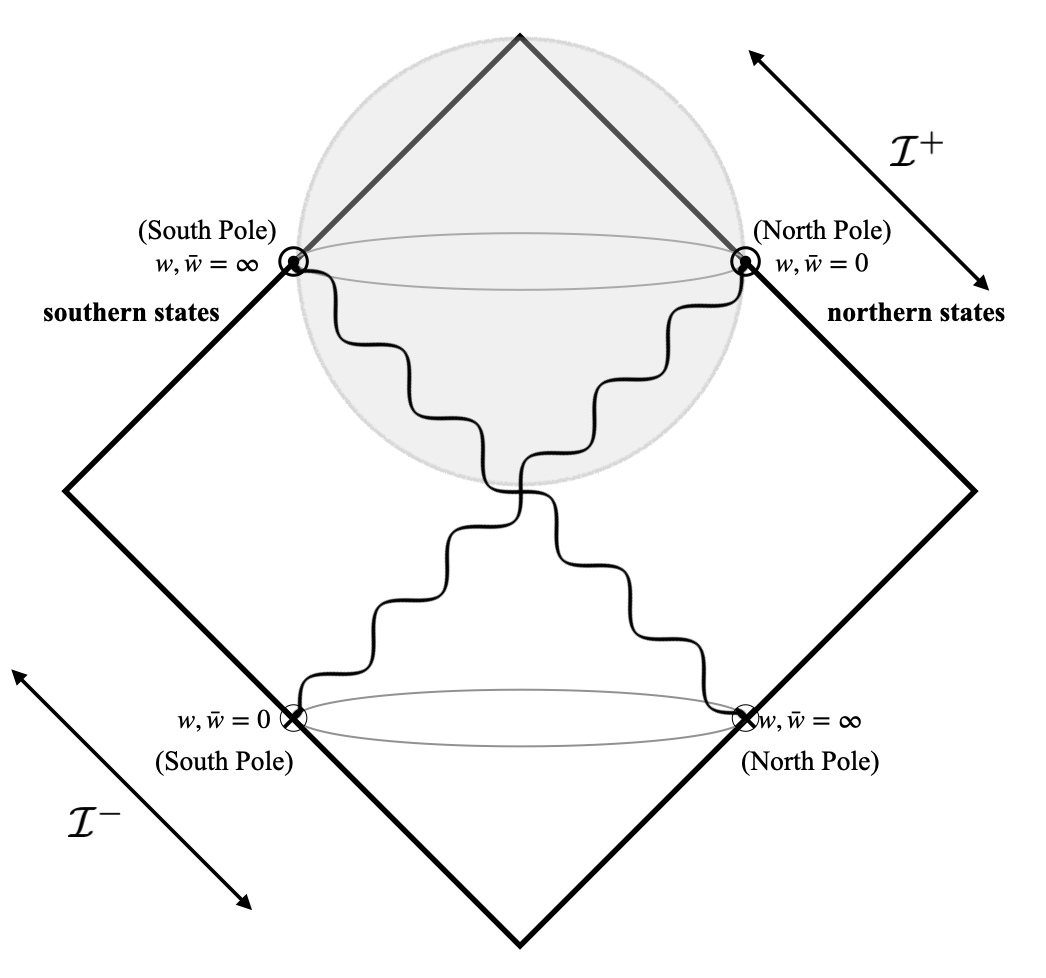
Figure 1: “Northern” states enter in the southern hemisphere on $\mathcal{I}^{-}$ and exit in the northern one on $\mathcal{I}^{+}$. “Southern” states enter in the northern hemisphere on $\mathcal{I}^{-}$ and exit in the southern one on $\mathcal{I}^{+}$. Due to the antipodal identification between the angular coordinates at $\mathcal{I}^{+}$ and $\mathcal{I}^{-}$, a free massless particle will enter and exit at the same point on the celestial sphere.

It will be useful to have a pictorial understanding of these states in relation to incoming and outgoing bulk particles. Massless particles enter at some point on $\mathcal{I}^{-}$ and exit at some point on $\mathcal{I}^{+}$. If we refer to $(w,\bar{w})=0$ as the south pole on ${\cal I}^{-}$ and, due to the antipodal matching, the north pole on ${\cal I}^{+}$, these 2D states describe particles which enter near the south pole on ${\cal I}^{-}$ and exit near the north pole on ${\cal I}^{+}$. All such excitations are north-moving and we will accordingly refer to these as “northern states” as shown Figure 1. Such a description cannot be used for states corresponding to south-moving particles entering (exiting) on the north (south) pole because they are at $(w,\bar{w})=\infty$ as shown in Figure 1. As we will see in the next section, such “southern states” are naturally viewed as “2D bra-states” rather than “2D ket-states”. We avoid using the term in- or out-states here in order to avoid confusion with the very different bulk notion of incoming or outgoing particles.

3.2 BPZ inner product in CCFT

In this section we show how the classic construction of BPZ [13] defines an indefinite 2D inner product for CCFT. Unfamiliar features arise since the fields have complex conformal weights. An operator acting on the bra-vacuum state $\langle 0_{2}|$ is defined starting with

$$\mathcal{B}^{\prime\pm,h,\bar{h}}(z,\bar{z})\equiv z^{2h}\bar{z}^{2\bar{h}}\mathcal{B}^{\pm,h,\bar{h}}(z,\bar{z}).$$ (3.11)

where $\mathcal{B}^{\pm,h,\bar{h}}$ is an arbitrary operator, notated as such to emphasize that it is distinct from the previously introduced $\mathcal{O}^{\pm,h,\bar{h}}$ and is associated with the bra-states. Defining $z^{\prime}=-\frac{1}{z}$, we see that $\left({\partial z\over\partial z^{\prime}}\right)^{h}\left({\partial\bar{z}\over\partial\bar{z}^{\prime}}\right)^{\bar{h}}\mathcal{B}^{\pm,h,\bar{h}}(z,\bar{z})$ is just the conformally transformed operator in $z^{\prime}$ coordinates which should be smooth for finite $z^{\prime}$. Hence the action of $\mathcal{B}^{\prime}$ must be finite when acting on $\langle 0_{2}|$ as $\frac{1}{z}\rightarrow 0$. This requires that the bra-states admit a mode expansion around $z=\infty$ in integer powers of $(z,\bar{z})$ as

$$\langle 0_{2}|\mathcal{B}^{\prime\pm,h,\bar{h}}(z,\bar{z})=\langle 0_{2}|\sum_{n,\bar{n}}\frac{\mathcal{B}^{\prime\pm,h,\bar{h}}_{n,\bar{n}}}{z^{n-h}\bar{z}^{\bar{n}-\bar{h}}},\ \ (n,\bar{n})\in\mathbb{Z}+(h,\bar{h}).$$ (3.12)

where we note the range of modes $(n,\bar{n})$ differs from the ket-state expansion (3.2). Again the modes are given by formal contour integrals

$$\langle 0_{2}|\mathcal{B}^{\prime\pm,h,\bar{h}}_{n,\bar{n}}=\frac{1}{(2\pi i)^{2}}\oint_{\infty}dz\oint_{\infty}d\bar{z}z^{n-h-1}\bar{z}^{\bar{n}-\bar{h}-1}\langle 0_{2}|{\mathcal{B}^{\prime}}^{\pm,h,\bar{h}}(z,\bar{z}),$$ (3.13)

where the contour integrals are taken around $z,\bar{z}=\infty$. Finally, a primary bra-state is defined as

$$\langle h,\bar{h},\pm|=\langle 0_{2}|\lim_{z,\bar{z}\rightarrow\infty}\mathcal{B}^{\prime\pm,h,\bar{h}}(z,\bar{z})=\langle 0_{2}|\mathcal{B}^{\prime\pm,h,\bar{h}}_{h,\bar{h}}.$$ (3.14)

For the state (3.12) to not diverge in this limit, we must have

$$\langle 0_{2}|\mathcal{B}^{\prime\pm,h,\bar{h}}_{n,\bar{n}}=0,\ \mbox{for}\ (n-h,\bar{n}-\bar{h})<0,$$ (3.15)

i.e. these serve as annihilation operators on $\langle 0_{2}|$.

In what follows, we will construct the inner product $\langle 0_{2}|{\mathcal{B}}^{\prime\pm h_{1},\bar{h}_{1}}_{n,\bar{n}}\mathcal{O}_{m,\bar{m}}^{\mp,h_{2},\bar{h}_{2}}|0_{2}\rangle$ by using the two-point function between $\mathcal{B}$ and $\mathcal{O}$ whose form, assuming $w_{1}\neq w_{2}$, is dictated by conformal invariance to be

$$\langle 0_{2}|\mathcal{B}^{\pm,h_{1},\bar{h}_{1}}(w_{1},\bar{w}_{1})\mathcal{O}^{\mp,h_{2},\bar{h}_{2}}(w_{2},\bar{w}_{2})|0_{2}\rangle=\frac{\mathcal{C}\delta_{h_{1},h_{2}}\delta_{\bar{h}_{1},\bar{h}_{2}}}{(w_{1}-w_{2})^{2h_{1}}(\bar{w}_{1}-\bar{w}_{2})^{2\bar{h}_{1}}}.$$ (3.16)

The constant $\mathcal{C}$ depends on the choice of operators but not on $w_{1}$ or $w_{2}$, and the expectation value is defined as the two-point scattering amplitude of the particles associated to the operators $\mathcal{B}$ and $\mathcal{O}$. For free field theory, as considered here, the 4D bulk momentum space scattering amplitude is the symplectic product of the corresponding plane waves up to a factor of $i$. Since Mellin transforms of 4D bulk momentum space scattering amplitudes are CCFT correlators, this two-point function equals, up to a factor of $i$, the symplectic product of the associated wavefunctions. Note that if we take $\mathcal{B}^{\pm,h,\bar{h}}=\mathcal{O}^{\mp,h,\bar{h}}$ the constant $\mathcal{C}$ vanishes, so the family of operators $\mathcal{O}^{\pm,h,\bar{h}}$ cannot be self-adjoint with respect to this inner product. In order for this to be nonzero we choose to use the shadow and take

$$\mathcal{B}^{\pm,h,\bar{h}}=\widetilde{\mathcal{O}}^{\pm,1-h,1-\bar{h}}.$$ (3.17)

One then has

$$\langle 0_{2}|\widetilde{\mathcal{O}}^{\pm,1-h_{1},1-\bar{h}_{1}}(w_{1},\bar{w}_{1})\mathcal{O}^{\mp,h_{2},\bar{h}_{2}}(w_{2},\bar{w}_{2})|0_{2}\rangle= \left(\phi_{\pm,h_{1},\bar{h}_{1}}^{\mu_{1}\ldots\mu_{s}}(X^{\mu};w_{1},\bar{w}_{1}),\phi_{\mp,h_{2},\bar{h}_{2}}^{\nu_{1}\ldots\nu_{s}}(X^{\mu};w_{2},\bar{w}_{2})\right)_{\mathcal{S}}$$ (3.18)

$$= \frac{\Gamma(2-2\bar{h}_{1})}{\pi\Gamma(2h_{1}-1)}\frac{\delta_{h_{1}+-\bar{h}_{1}+h_{2}-\bar{h}_{2}}\mathcal{C}_{J_{1}}^{\pm}(\lambda_{1})\delta(\lambda_{1}+\lambda_{2})}{(w_{1}-w_{2})^{2h_{2}}(\bar{w}_{1}-\bar{w}_{2})^{2\bar{h}_{2}}}.$$ (3.19)

So far we only have a formula for correlation functions of primary operators and their primary shadows at non-coincident points on the sphere. We seek an inner product on primary states and their descendants where the latter follows from the former in the usual manner [13]. If we insert modes of $\widetilde{\mathcal{O}}^{\prime}$ and $\mathcal{O}$ between vacuum states, we find

$$\langle 0_{2}|{\widetilde{\mathcal{O}}}^{\prime\pm,1-h_{1},1-\bar{h}_{1}}_{n,\bar{n}}\mathcal{O}_{m,\bar{m}}^{\mp,h_{2},\bar{h}_{2}}|0_{2}\rangle= \frac{1}{(2\pi i)^{4}}\oint_{\infty}dw_{1}\oint_{\infty}d\bar{w}_{1}w_{1}^{n+h_{1}-2}\bar{w}_{1}^{\bar{n}+\bar{h}_{1}-2}\oint_{0}dw_{2}\oint_{0}d\bar{w}_{2}w_{2}^{h_{2}+m-1}\bar{w}_{2}^{\bar{h}_{2}+\bar{m}-1}$$

$$\times w_{1}^{2(1-h_{1})}\bar{w}_{1}^{2(1-\bar{h}_{1})}\langle 0_{2}|\widetilde{\mathcal{O}}^{\pm 1-h_{1},1-\bar{h}_{1}}(w_{1},\bar{w}_{1})\mathcal{O}^{\mp,h_{2},\bar{h}_{2}}(w_{2},\bar{w}_{2})|0_{2}\rangle.$$ (3.20)

Inserting (3.18), and evaluating the integral using

$$\frac{1}{2\pi i}\oint dzz^{h+m-1}(w-z)^{-2h}=\frac{w^{m-h}\Theta(-h-m)\Gamma(h-m)}{\Gamma(1-h-m)\Gamma(2h)}$$ (3.21)

where $h+m\in\mathbb{Z},h\in\mathbb{C}$, we find that the inner product is

$$\langle 0_{2}|\widetilde{\mathcal{O}}^{\prime\pm,1-h_{1},1-\bar{h}_{1}}_{n,\bar{n}}\mathcal{O}_{m,\bar{m}}^{\mp,h_{2},\bar{h}_{2}}|0_{2}\rangle = \frac{\delta_{h_{1}-\bar{h}_{1}+h_{2}-\bar{h}_{2}}\mathcal{C}^{\pm}_{J_{1}}(\lambda_{1})\delta(\lambda_{1}+\lambda_{2})\Gamma(h_{2}-m)\Gamma(\bar{h}_{2}-\bar{m})}{\pi\Gamma(1-2h_{2})\Gamma(2h_{2})\Gamma(1-h_{2}-m)\Gamma(1-\bar{h}_{2}-\bar{m})}$$ (3.22)

$$\times \Theta(n-h_{2})\Theta(\bar{n}-\bar{h}_{2})\delta_{m+n}\delta_{\bar{m}+\bar{n}}.$$ (3.23)

Note that the above equation is only nonzero when $(h_{2},\bar{h}_{2})=(1-h_{1},1-\bar{h}_{1})$ and $(m,\bar{m})=(-n,-\bar{n})$. Therefore this formula identifies the adjoint of ${\mathcal{O}}^{\mp,h,\bar{h}}_{m,\bar{m}}|0_{2}\rangle$ as

$$\langle 0_{2}|\widetilde{\mathcal{O}}^{\prime\pm,h,\bar{h}}_{-m,-\bar{m}}=({\mathcal{O}}^{\mp,h,\bar{h}}_{m,\bar{m}}|0_{2}\rangle)^{\dagger}.$$ (3.24)

One can also show that the two-point function can be reconstructed via a sum over all the modes, providing a check that our basis of descendants is complete.

This inner product brings us full circle and can be easily connected to the the bulk analysis and shadow product in the previous section. If we consider the primary states (3.4) and (3.14), we see that the inner product we define here is

$$\langle 0_{2}|\widetilde{\mathcal{O}}^{\prime\pm,1-h_{1},1-\bar{h}_{1}}_{1-h_{1},1-\bar{h}_{1}}\mathcal{O}_{-h_{2},-\bar{h}_{2}}^{\mp,h_{2},\bar{h}_{2}}|0_{2}\rangle=\frac{\delta_{h_{1}-\bar{h}_{1}+h_{2}-\bar{h}_{2}}\mathcal{C}^{\pm}_{J_{1}}(\lambda_{1})\delta(\lambda_{1}+\lambda_{2})\Gamma(2\bar{h}_{2})}{\pi\Gamma(1-2h_{2})}.$$ (3.25)

Likewise we could have started with the bulk shadow product in (2.24), multiplied it by the conformal factor $w_{1}^{2(1-h_{1})}\bar{w}_{1}^{2(1-\bar{h}_{1})}$, thereby taking the first field to the opposite pole, and then taken the limit $w_{1},\bar{w}_{1}\rightarrow\infty$ and $w_{2},\bar{w}_{2}\rightarrow 0$ to obtain the same expression. This should not be surprising since it follows directly from the CCFT state-operator correspondence. The same connection exists for descendants since considering arbitrary modes in (3.22) will correspond to inserting $L_{-1}$ and $L_{1}$ in (2.24), multiplying by the appropriate conformal factor and taking the limit.

Since the inner product here is the standard BPZ product in CFT₂ it is manifest that $L_{n}^{\dagger}=L_{-n}$ and $\bar{L}_{n}^{\dagger}=\bar{L}_{-n}$, unlike the relation $L_{n}^{\dagger}=-\bar{L}_{n}$ encountered in the 4D bulk Klein-Gordon product. It is nevertheless instructive to derive the adjoint relations directly. As shown in Appendix A

$$\langle 0_{2}|[L_{-n}\mathcal{,}\widetilde{\mathcal{O}}^{\prime\mp,h,\bar{h}}_{-m,-\bar{m}}]=-((h-1)n-m)\langle 0_{2}|\widetilde{\mathcal{O}}^{\prime\mp,h,\bar{h}}_{-m-n,-\bar{m}}.$$ (3.26)

This allows us to compute $L_{n}^{\dagger}$ acting on the bra-state

$$\bra{0_{2}}\widetilde{\mathcal{O}}^{\prime\pm,h,\bar{h}}_{m,\bar{m}}L_{n}^{\dagger}=\left(L_{n}\mathcal{O}_{m,\bar{m}}^{\mp,h,\bar{h}}|0_{2}\rangle\right)^{\dagger}=((h-1)n-m)\left(\mathcal{O}^{\mp,h,\bar{h}}_{m+n,\bar{m}}\ket{0_{2}}\right)^{\dagger}=((h-1)n-m)\langle 0_{2}|\widetilde{\mathcal{O}}^{\prime\pm,h,\bar{h}}_{-m-n,-\bar{m}}$$ (3.27)

where in the second equality we used (3.9). If we compare the above equation with (3.26), we are able to conclude that

$$L_{n}^{\dagger}=L_{-n}$$ (3.28)

as promised.

This discussion could be traced backwards. Given that the BPZ construction implies the adjoint relation $L_{n}^{\dagger}=L_{-n}$, the inner products of descendants (3.22) then follows, up to an overall normalization, from the general SL$(2,\mathbb{C})$ relation (3.9).

4 Bulk versus boundary scattering

Thus far we have discussed the inner products of quantum states in free field theory, as well as the novel relation between the bulk products on 4D states and the boundary inner product on 2D states. Here we make some observations on the associated relation between the bulk and boundary scattering problems.

The bulk $N$-particle $\cal S$-matrix is a map $\cal{H}_{\rm in}\to\cal{H}_{\rm out}$ between a state in the incoming 4D Hilbert space on $\cal{I}^{-}$ and the outgoing Hilbert space on $\cal{I}^{+}$ as shown in the left panel of Figure 2. In a conformal basis, the incoming $N$-particle states are created on $\cal{I}^{-}$ by products of positive frequency operators ${\mathcal{O}}^{+,h_{k},\bar{h}_{k}}(w_{k},\bar{w}_{k})$, $k=1,..N_{\rm in}$, and are annihilated on $\cal{I}^{+}$ by products of negative frequency operators ${\mathcal{O}}^{-,h_{k},\bar{h}_{k}}(w_{k},\bar{w}_{k})$, $k=1,..N_{\rm out}$, with $N=N_{\rm in}+N_{\rm out}$. The operators $\mathcal{O}^{-}$ ($\mathcal{O}^{+}$) are associated to $\cal{I}^{+}$ ($\cal{I}^{-}$).

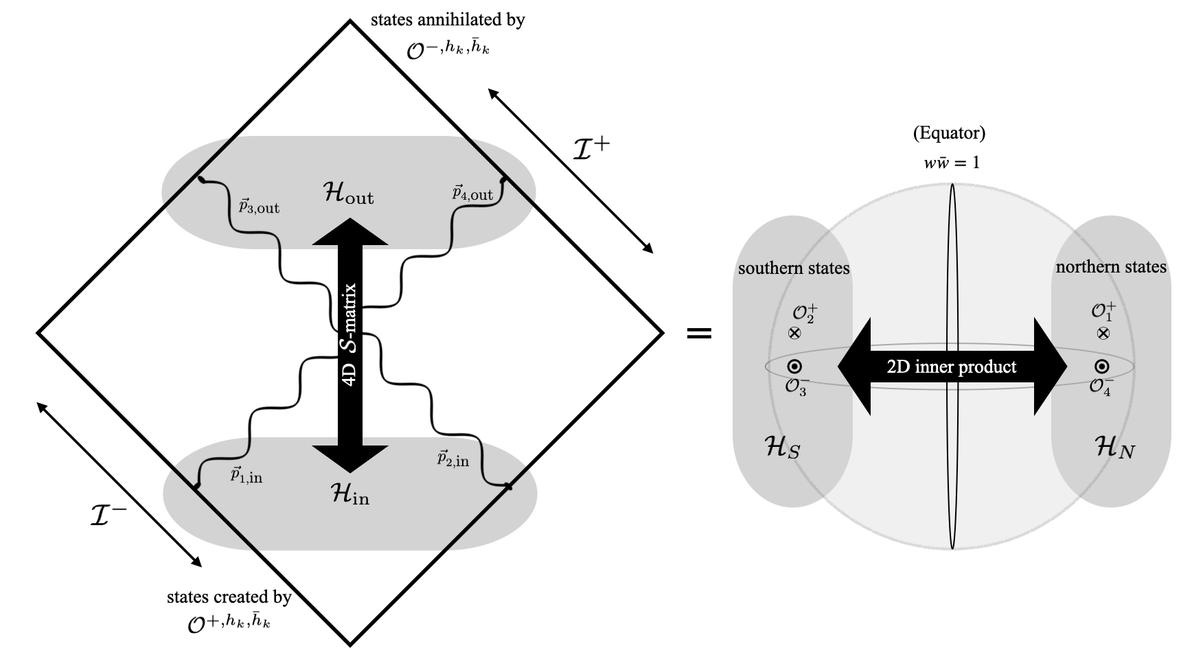
Figure 2: On the left we depict the 4D scattering problem. Incoming states are in the Hilbert space $\mathcal{H}_{\rm{in}}$ at $\mathcal{I}^{-}$ and outgoing states are in the Hilbert space $\mathcal{H}_{\rm{out}}$ at $\mathcal{I}^{+}$. The bulk scattering problem is to relate these two Hilbert spaces. On the right we depict the 2D scattering problem. In the northern (southern) hemisphere we have northern (southern) states, those originating at the south (north pole) of $\mathcal{I}^{-}$, and they form the Hilbert space $\mathcal{H}_{N}$ ($\mathcal{H}_{S}$). The dots represent operators that annihilate the northern (southern) states on $\mathcal{I}^{+}$ and the crosses represent antipodally mapped operators that create the northern (southern) states on $\mathcal{I}^{-}$. The boundary scattering problem is to find the overlap between the states in these two Hilbert spaces.

This same bulk $N$-particle $\cal S$-matrix can be expressed as a map between two 2D Hilbert spaces. To do so, we choose an equator on the celestial sphere. We take this to be $w\bar{w}=1$ in our conventions and refer to $w\bar{w}<1$ as the northern hemisphere and $w\bar{w}>1$ as the southern hemisphere as shown in the right panel of Figure 2. If there are no operator insertions on either hemisphere, starting from the vacuum at the north (south) pole, and evolving to the equatorial boundary of the northern (southern) hemisphere creates the vacuum state in the northern (southern) Hilbert space $\cal{H}_{\rm N}$ ($\cal{H}_{\rm S}$). If there are operator insertions at points on the hemispheres, evolution from the pole will create a corresponding state in the Hilbert space. Our inner product between states in either Hilbert space is then an $\cal S$-matrix element.

While the pairs $(\cal{H}_{\rm in},\cal{H}_{\rm out})$ and $(\cal{H}_{\rm N},\cal{H}_{\rm S})$ contain the same information, they clearly organize it quite differently. Whereas a single 4D Hilbert space contains either all the data on $\mathcal{I}^{+}$ or all the data on $\mathcal{I}^{-}$, a single 2D Hilbert space contains part of the data from $\mathcal{I}^{-}$ along with part of the data from $\mathcal{I}^{+}$. To see this, we should understand the operator insertions that appear on each 2D hemisphere. A single-particle 2D state in $\cal{H}_{\rm N}$ can either be associated to an operator ${\mathcal{O}}^{-,h_{k},\bar{h}_{k}}(w_{k},\bar{w}_{k})$ or ${\mathcal{O}}^{+,h_{k},\bar{h}_{k}}(w_{k},\bar{w}_{k})$ with $w_{k}\bar{w}_{k}<1$. The operator ${\mathcal{O}}^{-,h_{k},\bar{h}_{k}}(w_{k},\bar{w}_{k})$ annihilates a bulk particle on the northern hemisphere at $\mathcal{I}^{+}$ while ${\mathcal{O}}^{+,h_{k},\bar{h}_{k}}(w_{k},\bar{w}_{k})$ creates a north-moving bulk particle in the southern hemisphere at $\mathcal{I}^{-}$.

The bulk scattering problem can be phrased as: “Given an incoming state in $\cal{H}_{\rm in}$, what is the resulting outgoing state in $\cal{H}_{\rm out}$?” The boundary scattering problem is “Given a northern state in $\cal{H}_{\rm N}$, what is the resulting southern state in $\cal{H}_{\rm S}$?” The bulk interpretation of this second question is novel. Given the multi-particle state leaving the southern hemisphere of $\cal{I}^{-}$, as well as the multi-particle state arriving in the northern hemisphere of $\cal{I}^{+}$, one must then reconstruct the multi-particle state leaving the northern hemisphere of $\cal{I}^{-}$, as well as the one arriving in the southern hemisphere of $\cal{I}^{+}$.

While a product of conformal primary operator insertions at distinct northern points $(w_{k},\bar{w}_{k})$ creates a state in $\cal{H}_{\rm N}$ as one evolves from the north pole, it is often convenient in CFT₂ to consider instead arbitrary insertions of primary operators as well as their SL$(2,\mathbb{C})$ descendants. These transform simply under the action of $(L_{n},\bar{L}_{n})$, and can be written in the general form (3.10) of operators acting on $|0_{2}\rangle$. Scattering amplitudes can then be identified with inner products of these ket-states with the analogous bra-states.

In conclusion the bulk to boundary dictionary in flat holography is more subtle than its familiar AdS counterpart. The 2D boundary states live on an oriented circle in the celestial sphere and capture the information of both ingoing and outgoing bulk excitations which cross the celestial sphere inside this circle. The 2D boundary $\cal S$-matrix is a map from the 2D state on one side of the circle to the other, and corresponds to a bulk map determining south-to-north excitations from north-to-south ones. This is a significant reframing of the quantum gravity scattering problem in Minkowski space.

Appendix A Conformal generators on adjoint modes

In this section we will show how, for $n=0,\pm 1$, the action of $L_{n}$ and $L_{n}^{\dagger}$ on the modes $\mathcal{O}^{\mp,h,\bar{h}}_{m,\bar{m}}$ and $\widetilde{\mathcal{O}}^{\prime\pm,h,\bar{h}}_{-m,-\bar{m}}$ can be derived straight from the two-point function. This might seem like a peculiar exercise. However, we do this in order to establish that these equations apply in the CCFT case, where we start with the two-point function and then infer the properties of the Hilbert space from it.

Defining

$$\langle\widetilde{\mathcal{O}}^{\prime\pm}_{1}\mathcal{O}_{2}^{\mp}\rangle \equiv \langle 0_{2}|\widetilde{\mathcal{O}}^{\prime\pm,1-h_{1},1-\bar{h}_{1}}(w_{1},\bar{w}_{1})\mathcal{O}^{\mp,h_{2},\bar{h}_{2}}(w_{2},\bar{w}_{2})|0_{2}\rangle$$ (A.1)

$$= \frac{\Gamma(2\bar{h}_{2})\mathcal{C}^{\pm}_{J_{1}}(\lambda_{1})\delta(\lambda_{1}+\lambda_{2})}{\pi\Gamma(1-2h_{2})}\frac{w_{1}^{2h_{2}}\bar{w}_{1}^{2\bar{h}_{2}}\delta_{h_{1}+h_{2}-\bar{h}_{1}-\bar{h}_{2}}}{(w_{1}-w_{2})^{2h_{2}}(\bar{w}_{1}-\bar{w}_{2})^{2\bar{h}_{2}}}$$ (A.2)

via explicit computation one can show that

$$(h_{2}(n+1)w_{2}^{n}+w_{2}^{n+1}\partial_{w_{2}})\langle\widetilde{\mathcal{O}}^{\prime\pm}_{1}\mathcal{O}^{\mp}_{2}\rangle=-((1-h_{1})(n-1)w_{1}^{n}+w_{1}^{n+1}\partial_{w_{1}})\langle\widetilde{\mathcal{O}}^{\prime\pm}_{1}\mathcal{O}_{2}^{\mp}\rangle$$ (A.3)

holds for $n=0,\pm 1$. This can be thought of as performing the computation of $\langle\widetilde{\mathcal{O}}^{\prime\pm}_{1}L_{n}\mathcal{O}_{2}^{\mp}\rangle$ in two different ways, by acting $L_{n}$ on the right and on the left. This implies that

$$[L_{n},\widetilde{\mathcal{O}}^{\prime\pm,1-h,1-\bar{h}}(z,\bar{z})] = (1-h)(n-1)z^{n}\widetilde{\mathcal{O}}^{\prime\pm,1-h,1-\bar{h}}(z,\bar{z})+z^{n+1}\partial_{z}\widetilde{\mathcal{O}}^{\prime\pm,1-h,1-\bar{h}}(z,\bar{z})$$ (A.4)

if one also assumes that for $n=0,\pm 1$, $L_{n}$ annihilates the vacuum $\langle 0_{2}|L_{n}=0$. In a more standard operator derivation, the difference between the commutator of $L_{n}$ with $\mathcal{O}^{\pm,h,\bar{h}}(w,\bar{w})$ and $\mathcal{O}^{\prime\pm,h,\bar{h}}(z,\bar{z})$ is due to the definition of the out states, as

$$[L_{n},\mathcal{O}^{\prime\pm,h,\bar{h}}(z,\bar{z})]=z^{2h}\bar{z}^{2\bar{h}}[L_{n},\mathcal{O}^{\pm,h,\bar{h}}(z,\bar{z})].$$ (A.5)

Using the mode expansions gives the following relation for the modes

$$\langle 0_{2}|[L_{n}\mathcal{,}\widetilde{\mathcal{O}}^{\prime\pm,h,\bar{h}}_{-m,-\bar{m}}] = ((h-1)n+m)\langle 0_{2}|\widetilde{\mathcal{O}}^{\prime\pm,h,\bar{h}}_{-m+n,-\bar{m}}$$ (A.6)

for $n=0,\pm 1$. The above equation is used in the derivation of  (3.28), the adjoint equation $L_{n}^{\dagger}=L_{-n}$. In a standard unitary CFT, $h^{\dagger}=h$ because $h$ is real. However, as we have constructed an inner product which is not sesquilinear (where the dual state is complex conjugated) but instead bilinear, then the adjoint of a scalar is itself. In that case, $h^{\dagger}=h$ will be true even if $h$ is complex. This is indeed the case in our CCFT inner product, which is bilinear in the fields.

References

- [1] F. Cachazo and A. Strominger, “Evidence for a New Soft Graviton Theorem,” arXiv:1404.4091 [hep-th].
- [2] D. Kapec, V. Lysov, S. Pasterski, and A. Strominger, “Semiclassical Virasoro symmetry of the quantum gravity -matrix,” JHEP 08 (2014) 058, arXiv:1406.3312 [hep-th].
- [3] T. He, P. Mitra, and A. Strominger, “2D Kac-Moody Symmetry of 4D Yang-Mills Theory,” JHEP 10 (2016) 137, arXiv:1503.02663 [hep-th].
- [4] D. Kapec, P. Mitra, A.-M. Raclariu, and A. Strominger, “2D Stress Tensor for 4D Gravity,” Phys. Rev. Lett. 119 no. 12, (2017) 121601, arXiv:1609.00282 [hep-th].
- [5] A. Bagchi, R. Basu, A. Kakkar, and A. Mehra, “Flat Holography: Aspects of the dual field theory,” JHEP 12 (2016) 147, arXiv:1609.06203 [hep-th].
- [6] C. Cheung, A. de la Fuente, and R. Sundrum, “4D scattering amplitudes and asymptotic symmetries from 2D CFT,” JHEP 01 (2017) 112, arXiv:1609.00732 [hep-th].
- [7] S. Pasterski, S.-H. Shao, and A. Strominger, “Flat Space Amplitudes and Conformal Symmetry of the Celestial Sphere,” Phys. Rev. D96 no. 6, (2017) 065026, arXiv:1701.00049 [hep-th].
- [8] C. Cardona and Y.-t. Huang, “S-matrix singularities and CFT correlation functions,” JHEP 08 (2017) 133, arXiv:1702.03283 [hep-th].
- [9] S. Pasterski and S.-H. Shao, “Conformal basis for flat space amplitudes,” Phys. Rev. D96 no. 6, (2017) 065022, arXiv:1705.01027 [hep-th].
- [10] O. Aharony, S. S. Gubser, J. M. Maldacena, H. Ooguri, and Y. Oz, “Large N field theories, string theory and gravity,” Phys. Rept. 323 (2000) 183–386, arXiv:hep-th/9905111 [hep-th].
- [11] R. Bousso, A. Maloney, and A. Strominger, “Conformal vacua and entropy in de Sitter space,” Phys. Rev. D 65 (2002) 104039, arXiv:hep-th/0112218.
- [12] G. S. Ng and A. Strominger, “State/Operator Correspondence in Higher-Spin dS/CFT,” Class. Quant. Grav. 30 (2013) 104002, arXiv:1204.1057 [hep-th].
- [13] A. A. Belavin, A. M. Polyakov, and A. B. Zamolodchikov, “Infinite Conformal Symmetry in Two-Dimensional Quantum Field Theory,” Nucl. Phys. B 241 (1984) 333–380.
- [14] S. Ferrara, A. Grillo, G. Parisi, and R. Gatto, “The shadow operator formalism for conformal algebra. Vacuum expectation values and operator products,” Lett. Nuovo Cim. 4S2 (1972) 115–120.
- [15] D. Simmons-Duffin, “Projectors, Shadows, and Conformal Blocks,” JHEP 04 (2014) 146, arXiv:1204.3894 [hep-th].
- [16] W. Fan, A. Fotopoulos, S. Stieberger, T. R. Taylor, and B. Zhu, “Conformal Blocks from Celestial Gluon Amplitudes,” arXiv:2103.04420 [hep-th].
- [17] A. Ashtekar, ASYMPTOTIC QUANTIZATION: BASED ON 1984 NAPLES LECTURES. Bibliopolis, 1987.
- [18] A. Fotopoulos, S. Stieberger, T. R. Taylor, and B. Zhu, “Extended Super BMS Algebra of Celestial CFT,” arXiv:2007.03785 [hep-th].
- [19] S. A. Narayanan, “Massive Celestial Fermions,” JHEP 12 (2020) 074, arXiv:2009.03883 [hep-th].
- [20] L. Iacobacci and W. Mueck, “Conformal Primary Basis for Dirac Spinors,” Phys. Rev. D 102 no. 10, (2020) 106025, arXiv:2009.02938 [hep-th].
- [21] A. Atanasov, A. Ball, W. Melton, A.-M. Raclariu, and A. Strominger, “ Scattering and the Celestial Torus,” arXiv:2101.09591 [hep-th].
- [22] A. Guevara, E. Himwich, M. Pate, and A. Strominger, “Holographic Symmetry Algebras for Gauge Theory and Gravity,” arXiv:2103.03961 [hep-th].
- [23] E. Witten, “Quantum gravity in de Sitter space,” in Strings 2001: International Conference. 6, 2001. arXiv:hep-th/0106109.
- [24] D. L. Jafferis, A. Lupsasca, V. Lysov, G. S. Ng, and A. Strominger, “Quasinormal quantization in de Sitter spacetime,” JHEP 01 (2015) 004, arXiv:1305.5523 [hep-th].
- [25] H. Osborn, “Conformal Blocks for Arbitrary Spins in Two Dimensions,” Phys. Lett. B 718 (2012) 169–172, arXiv:1205.1941 [hep-th].
- [26] L. Donnay, A. Puhm, and A. Strominger, “Conformally Soft Photons and Gravitons,” JHEP 01 (2019) 184, arXiv:1810.05219 [hep-th].
- [27] A. Fotopoulos, S. Stieberger, T. R. Taylor, and B. Zhu, “Extended BMS Algebra of Celestial CFT,” arXiv e-prints (Dec, 2019) arXiv:1912.10973, arXiv:1912.10973 [hep-th].
- [28] P. Di Francesco, P. Mathieu, and D. Sénéchal, Conformal field theory. Graduate texts in contemporary physics. Springer, New York, NY, 1997. https://cds.cern.ch/record/639405.
- [29] G. ’t Hooft, “The Scattering matrix approach for the quantum black hole: An Overview,” Int. J. Mod. Phys. A 11 (1996) 4623–4688, arXiv:gr-qc/9607022.