Thermal gauge theories with Lagrange multiplier fields

Abstract

We study the Yang-Mills theory and quantum gravity at finite temperature, in the presence of Lagrange multiplier fields. These restrict the path integrals to field configurations which obey the classical equations of motion. This has the effect of doubling the usual one–loop thermal contributions and of suppressing all radiative corrections at higher loop order. Such theories are renormalizable at all temperatures. Some consequences of this result in quantum gravity are briefly examined.

I Introduction

The standard theory of quantum gravity, which is based upon the Einstein-Hilbert (EH) Lagrangian, is non-renormalizable tHooft:1974bx ; Goroff:1986th ; vandeVen:1991gw . It requires an infinite number of counterterms which involve higher-order terms in the curvature tensor, to cancel all the ultraviolet divergences Gomis:1995jp ; PhysRevD.100.026018 . Many studies have been devoted to obtain a quantum field theory that is renormalizable and unitary while having general relativity as a classical limit. These entail, for example, the introduction of additional terms and fields into the action, like higher derivatives models Mannheim:2011ds and supergravity Freedman:2012zz , or the appeal to non-perturbative properties of renormalization group functions Nagy:2012ef . These attempts have met with varying degrees of success. Moreover, it has been argued that quantum gravity may be an effective field theory obtained in the low energy limit of a string theory green_schwarz_witten_2012 ; polchinski_1998 .

Recently, it has been proposed that there may be an alternative way of quantizing the EH action that removes such divergences in a simpler manner, preserves unitarity and produces the expected tree level effects McKeon:1992rq ; PhysRevD.100.125014 ; Brandt:2018lbe ; McKeon:2020pkm ; Brandt:2021ycu . This involves the introduction of a Lagrangian multiplier (LM) field that restricts the path integral used to quantize the theory to paths that satisfy the classical Euler-Lagrange equations. One finds that this procedure yields, at zero temperature, twice the usual one–loop contributions and that all higher order radiative corrections vanish.

We are thus motivated to extend this analysis to quantum gravity with LM fields at finite temperature. However, since such calculations are rather involved, we will follow in this work Feynman’ s approach Klauder:1972lsv : “The algebraic complexity of the gravitational field equations is so great that it is very difficult to investigate it…The Yang-Mills theory is also a non-linear theory which might show the same kind of problems, and yet be easier to handle algebraically. This proved to be the case, and thereafter all the work was done first with the Yang–Mills theory and then the corresponding expressions for gravitation were worked out.” Thus, in section 2, we study the Yang-Mills theory with a Lagrange multiplier field at finite temperature Braaten:1990mz ; Frenkel:1989br ; lebellac:book96 ; kapusta . To this end, we introduce the method of forward scattering amplitudes Frenkel:1989br ; Barton:1990fk which greatly simplifies the computations. With these insights, we extend in section 3 the analysis to thermal quantum gravity with Lagrange multiplier fields. We find that, up to one–loop order, the thermal effects are twice those obtained in the usual theories, while all contributions beyond one–loop order are eliminated. In section 4, we present a short discussion of the results and their possible implications in quantum gravity.

II Thermal Yang-Mills theory with LM fields

The usual Yang-Mills (YM) theory is described by the Lagrangian

$${\cal L}_{YM}=-\frac{1}{4}f^{a}_{\mu\nu}f^{a\mu\nu};\;\;\;f_{\mu\nu}=\partial_{\mu}A_{\nu}^{a}-\partial_{\nu}A_{\mu}^{a}+gf^{abc}A_{\mu}^{b}A_{\nu}^{c},$$ (1)

where $A_{\mu}^{a}$ is the gauge field. The Lagrange multiplier (LM) $\lambda_{\mu}^{a}$ field is introduced as

$$\lambda_{\mu}^{a}\frac{\partial{{\cal L}_{YM}}}{\partial A^{a}_{\mu}}=-\lambda_{\mu}^{a}D^{ab}_{\nu}f^{b\mu\nu},$$ (2)

where $D^{ab}_{\nu}=\partial_{\nu}\delta^{ab}+gf^{acb}A^{c}_{\nu}$ is the covariant derivative. The gauge fixing terms in the Feynman gauge, together with the corresponding ghost terms, have the form

$$-\frac{1}{2}(\partial\cdot A)^{2}-(\partial\cdot A^{a})(\partial\cdot\lambda^{a})-{\bar{c}}^{a}\partial\cdot D^{ab}(A)d^{b}-{\bar{d}}^{a}\partial\cdot D^{ab}(A)c^{b}-{\bar{c}}^{a}\partial\cdot D^{ab}(A+\lambda)c^{b},$$ (3)

(see Eqs. (13) and (17) of McKeon:1992rq ) where $c$, $d$ and $\bar{c}$, $\bar{d}$ are respectively the ghost and anti-ghost fields. It may be verified that the complete Lagrangian is invariant under BRST transformations.

The quadratic part of the Lagrangian is

$${\cal L}^{(2)}=\frac{1}{2}\begin{pmatrix}A^{a\mu},&\lambda^{a\mu}\end{pmatrix}\begin{pmatrix}\partial^{2}&\partial^{2}\\ \partial^{2}&0\end{pmatrix}\begin{pmatrix}A^{a}_{\mu}\\ \lambda^{a}_{\mu}\end{pmatrix}-\begin{pmatrix}{\bar{c}}^{a},&{\bar{d}}^{a}\end{pmatrix}\begin{pmatrix}\partial^{2}&\partial^{2}\\ \partial^{2}&0\end{pmatrix}\begin{pmatrix}{c}^{a}\\ d^{a}\end{pmatrix}$$ (4)

which leads to the following matrix propagator

$$\Delta=\begin{pmatrix}\partial^{2}&\partial^{2}\\ \partial^{2}&0\end{pmatrix}^{-1}=\begin{pmatrix}0&1/\partial^{2}\\ 1/\partial^{2}&-1/\partial^{2}\end{pmatrix}.$$ (5)

We see that there is no $\langle AA\rangle$ propagator. There are, however, mixed $\langle A\lambda\rangle=\langle\lambda A\rangle$ propagators as well as a propagator $\langle\lambda\lambda\rangle$ for the LM field. Moreover, all vertices have at most a single LM field. As a result, one cannot draw a Feynman diagram with more than one loop. Consequently, no higher loop diagrams can contribute.

The starting point of the thermal field theory is the new definition of an observable $O$ for a system in contact with a thermal bath at temperature $T$

$$\langle O\rangle_{T}=Z^{-1}{\rm Tr}\left(e^{-H/T}\,O\right),$$ (6)

where $Z$ is the partition functionlebellac:book96 . The Boltzmann factor $\exp(-H/T)$ weights the occupation number of states that are accessible to the system. In the imaginary time formalism, in momentum space, a thermal quantum field theory in $3+1$ dimensions reduces to a $3$-dimensional Euclidean theory with an infinite summation over the Matsubara frequencies $Q^{0}_{n}=i2\pi nT$ ($n=0,\pm 1,\pm 2,\dots$ or $n=\pm 1/2,\pm 3/2,\pm 5/2$ for Bosons or Fermions respectively).

The thermal field theory is renormalizable, provided the zero-temperature theory is so. This is intuitively obvious as the thermal perturbative corrections come with a Bose-Einstein factor

$$N_{B}(\omega)=\frac{1}{e^{\omega/T}-1}$$ (7)

that cuts off any ultraviolet divergence.

II.1 Forward scattering amplitudes

In the imaginary time formalism, the Bosonic Matsubara summations can be done using the relation kapusta

$$T\sum_{n=-\infty}^{\infty}f(Q^{0}_{n})=\int_{-i\infty}^{i\infty}\frac{dQ^{0}}{2\pi i}\frac{f(Q^{0})+f(-Q^{0})}{2}+\int_{-i\infty+\delta}^{i\infty+\delta}\frac{dQ^{0}}{2\pi i}\frac{f(Q^{0})+f(-Q^{0})}{e^{Q^{0}/T}-1}$$ (8)

which allows us to separate the $T=0$ part (first term) from the finite-temperature contribution (second term).

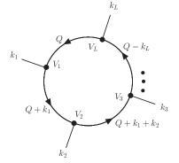
Figure 1: A generic one–loop diagram.

Using Eq. (8), the thermal part of a generic one-loop diagram containing a number $L$ of internal lines, as shown in Fig. 1, is given by

$$\int\,\frac{{\rm d}^{3}Q}{(2\pi)^{3}}\int_{-i\infty+\delta}^{i\infty+\delta}\frac{{\rm d}Q^{0}}{2\pi i}\,\frac{f(Q^{0},\vec{Q},k_{1},k_{2},\dots,k_{L})+f(-Q^{0},\vec{Q},k_{1},k_{2},\dots,k_{L})}{e^{Q^{0}/T}-1}.$$ (9)

$$= \int\,\frac{{\rm d}^{3}Q}{(2\pi)^{3}}\int_{-i\infty+\delta}^{i\infty+\delta}\frac{{\rm d}Q^{0}}{2\pi i}\,\frac{1}{e^{Q^{0}/T}-1}\left(f(Q^{0},\vec{Q},k_{1},k_{2},\dots,k_{L})+Q\leftrightarrow-Q\right).$$

From Eq. (5) we know that $f(Q^{0},\vec{Q},k_{1},k_{2},\dots,k_{L})$ has the following structure

$$f(Q^{0},\vec{Q},k_{1},k_{2},\dots,k_{L})=\frac{1}{{Q^{0}}^{2}-\vec{Q}^{2}}\frac{1}{(Q^{0}+k_{1}^{0})^{2}-(\vec{Q}+\vec{k}_{1})^{2}}\cdots\frac{t(Q,k_{1},k_{2}\cdots k_{L})}{(Q^{0}-k_{L}^{0})^{2}-(\vec{Q}-\vec{k}_{L})^{2}};\;\;\;(k_{1}+k_{2}+\cdots+k_{L}=0).$$ (10)

where $t(Q,k_{1},k_{2}\cdots k_{L})$ is a tensor (or a scalar in the case of a scalar field theory) which is determined by the interaction vertices of the theory. Using partial fraction decomposition like

$$\frac{1}{(Q^{0}+{k}^{0})^{2}-(\vec{Q}+\vec{k})^{2}}=\frac{1}{2\,|\vec{Q}+\vec{k}|}\left[\frac{1}{Q^{0}+k^{0}-|\vec{Q}+\vec{k}|}-\frac{1}{Q^{0}+k^{0}+|\vec{Q}+\vec{k}|}\right]$$ (11)

($(k^{0},\vec{k})$ represents any of the following possibilities: $(0,\vec{0})$, $(k^{0}_{1},\vec{k}_{1})$, $(k^{0}_{1}+k^{0}_{2},\vec{k}_{1}+\vec{k}_{2})$, $\dots$, $(-k^{0}_{l},-\vec{k}_{l})$) the $Q^{0}$ integral can be done upon closing the integration contour on the right hand side of the complex plane and using Cauchy’s integral formula. Then, performing shifts in the momentum $\vec{Q}$ and using the property $\exp(x+i2\pi m)=\exp(x)$; $m=0,\pm 1,\pm 2,\dots$, one can show that

$$\left[\begin{array}[]{l}\includegraphics[scale={0.5}]{one_loop.eps}\end{array}\right]_{\rm thermal}=-\int\,\frac{{\rm d}^{3}Q}{(2\pi)^{3}}\frac{1}{2|\vec{Q}|}\frac{1}{e^{|\vec{Q}|/T}-1}{\cal A}(Q,k_{1},k_{2},\cdots,k_{L}),$$ (12)

(the minus sign arises from the clockwise contour on the right hand complex plane) where

$${\cal A}(Q,k_{1},k_{2},\cdots,k_{L}) \equiv \left(\begin{array}[]{c}\includegraphics[scale={0.7}]{Nforward}\end{array}+Q\leftrightarrow-Q\right)_{Q^{0}=|\vec{Q}|}$$ (14)

$$+ \mbox{ cyclic permutations of }V_{1},V_{2},\dots,V_{L}.$$ (15)

The tree amplitude ${\cal A}(Q,k_{1},k_{2},\cdots,k_{L})$ is a forward scattering amplitude which describes the scattering of a on-shell particle of momentum $Q$ by external particles of momentum $k_{1}$, $k_{2}$, $\dots$, $k_{L}$ Barton:1990fk . It is a rational function of $k^{0}$ which can be analytically continued to all continuous values of the external energy.

One can now evaluate the leading high-temperature contributions, which come from the hard thermal region where $|\vec{Q}|\gg|\vec{k}_{i}|,|k^{0}_{i}|$. To this end, we expand the denominators of ${\cal A}(Q,k_{1},k_{2},\cdots,k_{L})$ as

$$\frac{1}{k^{2}+2k\cdot Q}=\frac{1}{2k\cdot Q}-\frac{k^{2}}{(2k\cdot Q)^{2}}+\dots.$$ (16)

($k$ represents any of the following possibilities: $k_{1}$, $k_{1}+k_{2}$, $\dots$, $-k_{L}$) After combining with the contributions from the numerator of ${\cal A}(Q,k_{1},k_{2},\cdots,k_{L})$, the expansions (16) produce terms of different degrees in $|\vec{Q}|$; the highest degree yields the leading high temperature behaviour, which can be found using the formula

$$\int_{0}^{\infty}d|\vec{Q}|\frac{|\vec{Q}|^{n-1}}{e^{|\vec{Q}|/T}-1}=\Gamma(n)\zeta(n)T^{n}$$ (17)

where $\zeta(n)$ is the Riemann zeta function.

Figure 2: One-loop contribution to the thermal self-energy of the gauge Boson. Springy lines represent the LM field; full lines denote the $d$ ghosts and traced lines represent the $c$ ghosts.

II.2 The gluon self-energy

Let us consider the contributions from the gluon self-energy diagrams shown in Fig. 2. These are twice those found in the usual YM theory, since in the later case there is a combinatorial factor of $1/2$ associated with purely gluonic graphs and only one type of ghost. Using Eqs. (14) and (12), we can write the thermal contribution from Fig. (2a) as

$${\Pi^{(1)}}^{ab}_{\mu\nu}(k)=-\int\frac{d^{3}Q}{(2\pi)^{3}}\frac{N_{B}(|\vec{Q}|)}{2|\vec{Q}|}{{\cal A}^{(1)}}^{ab}_{\mu\nu}(Q,k),$$ (18)

where the forward scattering amplitude ${{\cal A}^{(1)}}^{ab}_{\mu\nu}(Q,k)$ is shown in Fig. (3a) (added with the permutation $(\mu\leftrightarrow\nu,k\leftrightarrow-k)$ and $Q\leftrightarrow-Q$).

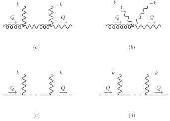
Figure 3: The forward scattering amplitudes corresponding to Fig. 2. Diagrams (a), (c) and (d) have to be added with $(\mu\leftrightarrow\nu,k\leftrightarrow-k)$ as well as $Q\leftrightarrow-Q$ as indicated in the Eq. (14).

Next, let us consider the thermal contribution from the tadpole graph shown in Fig. (2b). Proceeding as before, we can express it in terms of the forward scattering amplitude as indicated in Fig. (3 b). Finally, we must consider the thermal contributions associated with the ghost loops shown in Figs. (2 c) and (2 d). These may also be expressed in terms of the forward scattering amplitudes shown in Figs. (3 c) and (3 d) together with the graphs obtained by making $(\mu\leftrightarrow\nu,k\leftrightarrow-k,Q\leftrightarrow-Q)$.

Denoting by ${\cal A}^{ab}_{\mu\nu}(Q,k)$ the total forward scattering amplitude, we can express the complete thermal contribution as

$$\Pi^{ab}_{\mu\nu}(k)=-\int\frac{d^{3}Q}{(2\pi)^{3}}\frac{N_{B}(|\vec{Q}|)}{2|\vec{Q}|}{\cal A}^{ab}_{\mu\nu}(Q,k).$$ (19)

Using the expansion of Eq. (16) and the formula (17), we find for the leading thermal contribution from the gluon self-energy, the expression

$$\Pi^{ab}_{\mu\nu}(k)=\frac{1}{3}g^{2}C_{A}T^{2}\delta^{ab}\int\frac{d\Omega}{4\pi}\left(\frac{k_{\mu}\hat{Q}_{\nu}+k_{\nu}\hat{Q}_{\mu}}{k\cdot\hat{Q}}-\frac{k^{2}}{(k\cdot\hat{Q})^{2}}\hat{Q}_{\mu}\hat{Q}_{\nu}-\eta_{\mu\nu}\right),$$ (20)

where ${\hat{Q}}=(1,{\vec{Q}}/{|\vec{Q}|})$ and $C_{A}$ is the group factor. Eq. (20) satisfies the transversality condition $k^{\mu}\Pi^{ab}_{\mu\nu}(k)=0$.

Finally, upon using identities for the integral over the directions $\vec{Q}/|\vec{Q}|$ Eq. (20) can be further simplified, yielding Brandt:1993mj

$$\Pi^{ab}_{\mu\nu}(k)=\frac{2}{3}C_{A}g^{2}T^{2}\delta^{ab}\int\frac{d\Omega}{4\pi}\left(k_{0}\frac{{\hat{Q}}_{\mu}{\hat{Q}}_{\nu}}{k\cdot{\hat{Q}}}-\eta_{\mu 0}\eta_{\nu 0}\right).$$ (21)

This result leads to a screening thermal mass squared given by

$$m^{2}=\frac{2}{3}C_{A}g^{2}T^{2},$$ (22)

which is twice that obtained in the usual YM theory lebellac:book96 , as expected.

III Thermal Quantum Gravity with LM fields

Next, let us consider the Einstein-Hilbert (EH) Lagrangian

$${\cal L}_{EH}=\frac{1}{\kappa^{2}}\sqrt{-g}g^{\mu\nu}R_{\mu\nu}(\Gamma),$$ (23)

where $\kappa$ is related to Newton’s constant $G$ as $\kappa=\sqrt{16\pi G}$ and the Christoffel symbol is

$$\Gamma^{\lambda}_{\mu\nu}=\frac{1}{2}g^{\lambda\sigma}\left(g_{\mu\sigma,\nu}+g_{\nu\sigma,\mu}-g_{\mu\nu,\sigma}\right).$$ (24)

The tensor $R_{\mu\nu}$ is given by

$$R_{\mu\nu}(\Gamma)=\Gamma^{\rho}_{\mu\rho,\nu}-\Gamma^{\rho}_{\mu\nu,\rho}+\Gamma^{\rho}_{\mu\sigma}\Gamma^{\sigma}_{\nu\rho}-\Gamma^{\sigma}_{\mu\nu}\Gamma^{\rho}_{\sigma\rho}.$$ (25)

For our purpose, it is convenient to expand the metric tensor $g^{\mu\nu}$ in terms of the deviation from the Minkowski metric $\eta^{\mu\nu}$ as follows

$$\sqrt{-g}g^{\mu\nu}=\eta^{\mu\nu}+\kappa h^{\mu\nu}.$$ (26)

This allows to evaluate perturbatively the thermal Green’ s functions by expanding the EH Lagrangian in powers of $\kappa$.

The Lagrange multiplier field $\Lambda^{\mu\nu}$ is introduced as

$$\Lambda^{\mu\nu}\frac{\partial{\cal L}_{EH}}{\partial h^{\mu\nu}}=\frac{2}{\kappa}\Lambda^{\mu\nu}R^{l}_{\mu\nu}+{\cal O}(\kappa),$$ (27)

where $R^{l}_{\mu\nu}$ is the linearized Ricci tensor.

It is simpler to work in the de Donder gauge by choosing the gauge fixing Lagrangian

$${\cal L}_{\rm fix}=(\partial_{\mu}h^{\mu\nu})^{2}-\Lambda^{\mu\nu}\left(\partial_{\mu}\partial_{\sigma}h^{\sigma}_{\;\nu}+\partial_{\nu}\partial_{\sigma}h^{\sigma}_{\;\mu}\right),$$ (28)

which leads to a contribution of the gravitational ghosts given by

$${\cal L}_{\rm ghost} = {\bar{c}}_{\nu}\partial^{2}\eta^{\mu\nu}d_{\mu}+\kappa{\bar{c}}_{\nu}\partial_{\mu}\left[h^{\mu\rho}\partial_{\rho}d^{\nu}+h^{\nu\rho}\partial_{\rho}d^{\mu}-\partial_{\rho}(h^{\mu\nu}d^{\rho})\right]+\{\bar{c}\rightarrow\bar{d},\;\;d\rightarrow c\}$$ (29)

$$+ {\bar{c}}_{\nu}\partial^{2}\eta^{\mu\nu}c_{\mu}+\kappa{\bar{c}}_{\nu}\partial_{\mu}\left[(h^{\mu\rho}+\Lambda^{\mu\rho})\partial_{\rho}c^{\nu}+(h^{\nu\rho}+\Lambda^{\nu\rho})\partial_{\rho}c^{\mu}-\partial_{\rho}((h^{\mu\nu}+\Lambda^{\mu\nu})c^{\rho})\right].$$

Using a similar procedure to that employed in the YM theory, it turns out that there is no $\langle hh\rangle$ propagator. There are, however, mixed $\langle h\Lambda\rangle=\langle\Lambda h\rangle$ propagators as well as a propagator $\langle\Lambda\Lambda\rangle$ for the LM fields, which have the form

$$D{}^{h}_{\alpha\beta,}{}^{\Lambda}_{\mu\nu}(Q)=-D{}^{\Lambda}_{\alpha\beta,}{}^{\Lambda}_{\mu\nu}(Q)=\frac{1}{2}\frac{1}{Q^{2}}\left(\eta_{\alpha\mu}\eta_{\beta\nu}+\eta_{\alpha\nu}\eta_{\beta\mu}-\eta_{\mu\nu}\eta_{\alpha\beta}\right).$$ (30)

As in the YM theory, all the radiative corrections in quantum gravity with LM fields vanish beyond the one–loop order. The Feynman diagrams which contribute to the one–loop graviton self-energy function are shown in Fig. 2. The associated forward scattering amplitudes of a thermal graviton with on-shell momenta are indicated in Fig. 3. As we have seen, such amplitudes must be multiplied by the corresponding Bose-Einstein factor and integrated over the 3-momentum. In this way, we can express the thermal self-energy graviton function as

$$\Pi_{\alpha\beta,\mu\nu}(k)=\frac{1}{4\pi^{2}}\int_{0}^{\infty}dQ|\vec{Q}|N_{B}(|\vec{Q}|)\int\frac{d\Omega}{4\pi}{\cal A}_{\alpha\beta,\mu\nu}(Q,k).$$ (31)

The leading high-temperature limit of the forward scattering amplitude ${\cal A}_{\alpha\beta,\mu\nu}(Q,k)$ is governed by the contributions quadratic in $Q$, for large values of $Q$. To obtain these, one needs to expand the Feynman denominators as shown in Eq. (16). Using the formula (17) we find that

$${\Pi}_{\alpha\beta,\mu\nu}(k)=\frac{\pi^{2}T^{4}}{60}\int\frac{d\Omega}{4\pi}{\cal A}_{\alpha\beta,\mu\nu}(\hat{Q},k),$$ (32)

where the forward amplitude ${\cal A}_{\alpha\beta,\mu\nu}(\hat{Q},k)$ is given by the expression (${\hat{Q}}=(1,{\vec{Q}}/{|\vec{Q}|})$)

$${\cal A}_{\alpha\beta,\mu\nu}(\hat{Q},k) = 2\kappa^{2}\left[\frac{k_{\nu}{\hat{Q}}_{\alpha}{\hat{Q}}_{\beta}{\hat{Q}}_{\mu}}{k\cdot{\hat{Q}}}+\frac{k_{\mu}{\hat{Q}}_{\alpha}{\hat{Q}}_{\beta}{\hat{Q}}_{\nu}}{k\cdot{\hat{Q}}}+\frac{k_{\alpha}{\hat{Q}}_{\beta}{\hat{Q}}_{\mu}{\hat{Q}}_{\nu}}{k\cdot{\hat{Q}}}\right.$$ (33)

$$+ \left.\frac{k_{\beta}{\hat{Q}}_{\alpha}{\hat{Q}}_{\mu}{\hat{Q}}_{\nu}}{k\cdot{\hat{Q}}}-\frac{k^{2}{\hat{Q}}_{\alpha}{\hat{Q}}_{\beta}{\hat{Q}}_{\mu}{\hat{Q}}_{\nu}}{(k\cdot{\hat{Q}})^{2}}\right]$$

The expression (32) is consistent with the Ward identity relating the self–energy to the one–particle graviton function $\Gamma_{\mu\nu}$ Brandt:1993dk :

$$(2\eta^{\alpha\lambda}k^{\beta}-\eta^{\alpha\beta}k^{\lambda})\Pi_{\alpha\beta,\mu\nu}(k)=-\kappa(k_{\mu}\Gamma_{\nu}^{\;\lambda}+k_{\nu}\Gamma_{\mu}^{\;\lambda})$$ (34)

which follows in consequence of the invariance under general coordinate transformations.

We note that the result (32) yields a screening thermal graviton mass squared given by

$$m_{g}^{2}=2(32\pi G)\frac{\pi^{2}T^{4}}{45},$$ (35)

which is twice that obtained in thermal quantum gravity Rebhan:1990yr .

Figure 4: Feynman diagrams contributing to the thermal three-graviton vertex function (a), and the associated forward scattering amplitudes (b). Graphs obtained by cyclic permutations of external gravitons are to be understood.

One can also evaluate the leading $T^{4}$ temperature corrections of the thermal three-point graviton function. A typical Feynman diagram is shown in Fig. (4a), while the corresponding forward scattering amplitude is indicated in Fig. (4b). This calculation is much more involved, but the result for the total forward scattering amplitude turns out to be twice that obtained in the usual quantum gravity theory Brandt:1993dk .

IV Discussion

We have examined the YM and quantum gravity theories with Lagrange multiplier fields at finite temperature. We have shown that the one–loop thermal contributions are twice those obtained in the usual theories, with all higher–order radiative corrections being suppressed. Such theories are renormalizable at all temperatures, as well as unitary. In the present theory, the Lagrange multiplier fields are regarded as being dynamical fields. It can be shown that this approach leads to a unitary theory with a positive energy spectrum, where the Lagrange multiplier particles appear asymptotically only in pairs Brandt:2021ycu . Such a feature is reminiscent of that observed in the case of the strange particles, which are produced by strong interactions only pairwise. Since the Lagrange multiplier theory reduces to Einstein’s theory in the classical limit at zero temperature McKeon:1992rq ; PhysRevD.100.125014 ; Brandt:2018lbe ; McKeon:2020pkm ; Brandt:2021ycu , it is compatible with general relativity in the low energy domain.

However, unlike the case at zero temperature, the thermal zeroth order effects also appear to be twice those obtained in the conventional gauge theories. This may be seen, for instance, by considering the partition function $Z$ in the Yang-Mills theory which, in the free-field case, is given by lebellac:book96

$$Z^{(0)}=\det\Delta={\det}^{2}\left(\frac{1}{\partial^{2}}\right)=\exp\left[2{\rm Tr}\ln\left(\frac{1}{\partial^{2}}\right)\right],$$ (36)

where $\Delta$ is the matrix propagator of Eq. (5). This leads to a radiation pressure

$$P=\frac{T}{V}\ln Z^{(0)}=2\frac{\pi^{2}T^{4}}{45},$$ (37)

which is twice that found in the usual gauge theories. This fact is due to the extra degrees of freedom associated with the LM field. This outcome depends only on the total number of degrees of freedom, so that the same result would also be obtained in quantum gravity. Thus, one may inquire about some possible implications of this fact in gravity. For example, in a star, it is the pressure of the electromagnetic radiation emitted during the carbon cycle that equilibrates the weight of the matter. In this case, the pressure of the gravitational radiation is negligible. Moreover, in the present epoch, the contribution of the pressure to the stress tensor for the matter distribution on a large scale, can be disregarded.

The LM field interacts with gravitons, but it does not directly couple to matter Brandt:2021ycu . Hence, such a field exhibits a behaviour resembling that of dark matter, which has gravitational interactions but does not otherwise couple to ordinary matter. Thus, the LM field may provide an extra gravity which could possibly affect the galactic dynamics.

Certainly, the only way of deciding the correctness of any approach to quantizing gravity is to appeal to experiment. Although such observations are not yet feasible, there have been several proposals for quantum gravity phenomenology. These include, for example, possible observations of quantum gravity effects in the cosmic microwave background Akhmedov2014 and of quantum decoherence induced by space-time fluctuations Oniga:2017pyq . It may be worth studying further the predictions of quantum gravity theories for such phenomena, which could be tested in the foreseeable future.

- (1) G. ’t Hooft and M. J. G. Veltman, Annales Poincare Phys. Theor. A20, 69 (1974).
- (2) M. H. Goroff and A. Sagnotti, Nucl. Phys. B266, 709 (1986).
- (3) A. E. M. van de Ven, Nucl. Phys. B378, 309 (1992).
- (4) J. Gomis and S. Weinberg, Nucl. Phys. B 469, 473 (1996).
- (5) P. M. Lavrov and I. L. Shapiro, Phys. Rev. D 100, 026018 (2019).
- (6) P. D. Mannheim, Found. Phys. 42, 388 (2012).
- (7) D. Z. Freedman and A. Van Proeyen, Supergravity (Cambridge Univ. Press, Cambridge, UK, 2012).
- (8) S. Nagy, Annals Phys. 350, 310 (2014).
- (9) M. B. Green, J. H. Schwarz, and E. Witten, Superstring Theory, Cambridge Monographs on Mathematical Physics (Cambridge University Press, Cambridge, 2012).
- (10) J. Polchinski, String Theory, Cambridge Monographs on Mathematical Physics (Cambridge University Press, Cambridge, 1998).
- (11) D. G. C. McKeon and T. N. Sherry, Can. J. Phys. 70, 441 (1992).
- (12) D. G. C. McKeon, F. T. Brandt, J. Frenkel, and G. S. S. Sakoda, Phys. Rev. D 100, 125014 (2019).
- (13) F. Brandt, J. Frenkel, and D. McKeon, Canadian Journal of Physics 98, 344 (2020).
- (14) F. T. Brandt, J. Frenkel, S. Martins-Filho, and D. G. C. McKeon, Annals Phys. 427, 168426 (2021).
- (15) F. T. Brandt, J. Frenkel, S. Martins-Filho, and D. G. C. McKeon, arXiv 2102.02854 (2021).
- (16) R. P. Feynman, in Magic Without Magic: John Archibald Wheeler: A Collection of Essays in Honor of his Sixtieth Birthday, edited by J. R. Klauder (Freeman, San Francisco, 1972).
- (17) E. Braaten and R. D. Pisarski, Nucl. Phys. B337, 569 (1990); Nucl. Phys. B339, 310 (1990).
- (18) J. Frenkel and J. C. Taylor, Nucl. Phys. B334, 199 (1990); Nucl. Phys. B374, 156 (1992).
- (19) F. T. Brandt, J. Frenkel, J. C. Taylor and S. M. H. Wong, Can. J. Phys. 71, 219-226 (1993).
- (20) M. L. Bellac, Thermal Field Theory (Cambridge University Press, Cambridge, England, 1996).
- (21) J. I. Kapusta, Finite Temperature Field Theory (Cambridge University Press, Cambridge, England, 1989).
- (22) G. Barton, Ann. Phys. 200, 271 (1990).
- (23) A. Rebhan, Nucl. Phys. B 351, 706-734 (1991).
- (24) F. T. Brandt and J. Frenkel, Phys. Rev. D47, 4688 (1993); Phys. Rev. D48, 4940 (1993).
- (25) E. T. Akhmedov, S. Minter, P. Nicolini, and D. Singleton, Advances in High Energy Physics 2014, 192712 (2014).
- (26) T. Oniga and C. H. T. Wang, Phys. Rev. D 96, 084014 (2017).