Bayesian Inference of a Dependent Competing Risk Data

Abstract

Analysis of competing risks data plays an important role in the lifetime data analysis. Recently Feizjavadian and Hashemi (Computational Statistics and Data Analysis, vol. 82, 19-34, 2015) provided a classical inference of a competing risks data set using four-parameter Marshall-Olkin bivariate Weibull distribution when the failure of an unit at a particular time point can happen due to more than one cause. The aim of this paper is to provide the Bayesian analysis of the same model based on a very flexible Gamma-Dirichlet prior on the scale parameters. It is observed that the Bayesian inference has certain advantages over the classical inference in this case. We provide the Bayes estimates of the unknown parameters and the associated highest posterior density credible intervals based on Gibbs sampling technique. We further consider the Bayesian inference of the model parameters assuming partially ordered Gamma-Dirichlet prior on the scale parameters when one cause is more severe than the other cause. We have extended the results for different censoring schemes also.

Key Words and Phrases: Marshall-Olkin bivariate Weibull distribution; Gamma-Dirichlet distribution; Bayes estimates; Competing Risk; Order Restricted Inference.

1 Introduction

In lifetime data analysis an experimenter often wants to analyze data which have multiple failure modes. In the statistical literature it is known as the competing risks problem. There are mainly two different approaches to handle competing risks data. One is known as the latent failure time model of Cox (1959) and the other is known as the cause specific hazard rate model of Prentice et al. (1978). In case of exponential and Weibull lifetime distributions it has been shown by Kundu (2004) that both the models lead to the same likelihood function, although their interpretations are different. An extensive list of literature exits in this area, see for example Kalbfleish and Prentice (1980), Lawless (1982) or Crowder (2001) and the references cited therein. Most of the existing studies are based on the assumptions that the causes of failures are independent, although it may not be true in practice. It may be mentioned that there are some identifiability issues in this respect, see for example Tsiatis (1975).

The bivariate or multivariate lifetime distributions play an important role in analyzing dependent competing risk model. Bayesian inference of a dependent competing risk model assuming absolute continuous bivariate exponential distribution is studied by Wang and Ghosh (2003). When there is a positive probability of simultaneous occurrence of two causes of failure then Marshall-Olkin bivariate exponential (MOBE) distribution, introduced by Marshall and Olkin (1967), can be used to analyze the data. If the data indicate that the marginals have unimodal probability density functions (PDFs) then MOBE distribution will not fit the data. Due to this limitations, Marshall-Olkin bivariate Weibull (MOBW) distribution was introduced by Lu (1989). Later this distribution has been studied by several authors including Jose, Ristic and Joseph (2011), Dey and Kundu (2009) and Kundu and Gupta (2013). The analysis of dependent competing risk model using MOBW distribution is considered by Feizjavdian and Hashemi (2015). Bayesian inference of a series system with dependent causes of failure using MOBW distribution is provided by Xu and Zhou (2017). Different methods of estimating parameters of dependent competing risks using MOBW model has been studied by Shen and Xu (2018).

Order restriction among model parameters in a reliability model has been considered by several authors. Order restricted inference of step-stress model has been considered by Balakrishnan, Beutner and Kateri (2009) and Samanta and Kundu (2018) to incorporate the fact that the increased stress level will reduce the expected lifetime of the experimental units. Recently Mondal and Kundu (2020) considered order restricted inference for two exponential populations. They have mentioned that this order restricted inference can be used in an accelerated life test if one sample is put under higher stress keeping the other one in normal stress. In competing risk model when it is known apriori that one cause of failure is higher risk than the other then we may incorporate this information by considering an order restriction on the model parameters.

The motivation of this paper came from a recent paper by Feizjavdian and Hashemi (2015). They have analyzed a data set obtained from the Diabetic Retinopathy Study (DRS) conducted by the National Eye Institute to estimate the effect of laser treatment in delaying the onset of blindness in patients with diabetic retinopathy. At the beginning of the experiment, for each patient, one eye was selected for laser treatment and the other eye was not given the laser treatment. For each patient the minimum time to blindness ($T$) and the indicator specifying whether the treated eye ($\delta$ = 1) or the untreated eye ($\delta$ = 2) has first failed has been recorded. If both the eyes have failed simultaneously then $\delta$ = 0 has been recorded. The data set is presented in Table 1. The main objective of this experiment is to study whether the laser treatment has any effect on delaying the onset of blindness in patients with diabetic retinopathy. Clearly, the time to blindness of the two eyes cannot be independent and there are some ties in the data set. Due to this reason Feizjavdian and Hashemi (2015) considered a dependent competing risks model and they have proposed to use the Marshall-Olkin bivariate Weibull distribution for this purpose. They provided the maximum likelihood estimators (MLEs) of the unknown parameters and obtained the associated asymptotic confidence intervals. The maximum likelihood estimators cannot be obtained in explicit forms, hence they have obtained the approximate maximum likelihood estimators which can be obtained in explicit forms. It is observed that the proposed model works quite well for fitting purposes. They have observed that even for highly censored data, the MLEs perform quite well.

The main aim of this paper is to provide the Bayesian analysis of the same data set under a very flexible Gamma-Dirichlet (GD) prior on the scale parameters and for a very general log-concave prior on the shape parameter. It is observed that the Bayesian inference has some natural advantages in this case. The Gamma-Dirichlet prior was originally introduced by Pena and Gupta (1990) for Marshall-Olkin bivariate exponential distribution (MOBE). The GD prior is a very flexible prior, and its joint PDF can take variety of shapes depending on the hyper parameters. It can be both positively and negatively correlated. In case of MOBW distribution the GD distribution is a conjugate prior of the scale parameters for a fixed shape parameter. Hence the posterior distribution of the scale parameters for the fixed shape parameter can be obtained in a very convenient form. We have used a very general log-concave prior on the shape parameter, and they are assumed to be independent. The Bayes estimators cannot be obtained in closed form. We have used Gibbs sampling technique to compute the Bayes estimates and the associated highest posterior density (HPD) credible intervals.

We further consider the Bayesian inference of the model parameters with partially order restriction on scale parameters. This order restriction comes naturally when it is apriori known that one cause of failure is more severe than the other. In this case we consider partially order restricted Gamma-Dirichlet prior for scale parameters and we use importance sampling technique for Bayes estimates and the credible intervals. We re-analyze the same data set assuming the order restriction on scale parameters. One major advantage of the Bayesian inference is that different forms of data for example; Type-I, Type-II, hybrid censored data can be handled quite conveniently also, unlike the classical inference. Finally the Bayesian testing of hypothesis has been considered to test the hypothesis that there is no significant difference between two causes of failure. We propose to use Bayes factor to test the hypothesis and interestingly in this case it can be obtained in explicit form. We have reanalyzed the data set and it is observed that the laser treatment does not have any effect in delaying the onset of blindness.

The rest of the paper is organized as follows. In Section 2 we describe the Marshall-Olkin bivariate Weibull distribution and provide the likelihood function based on competing risk data. Prior assumptions and posterior analysis is provided in Section 2.1. The order restricted Bayesian inference is given in Section 3. The inference under different censoring scheme is provided in Section 4. In Section 5, we discuss the Bayesian testing of hypothesis problem. The analysis of the data set has been provided in Section 6 and an extensive simulation results have been discussed in Section 7. Finally we have concluded the article in Section 8.

2 Marshal-Olkin Bivariate Weibull Competing Risk Model

Suppose a life testing experiment starts with $n$ number of identical units at time zero and the failure times are recorded. We assume that the units are failed due to several causes of failure. Here we restrict ourselves to two causes of failure, although the results can be easily generalized for more than two causes also. Let $X_{1}$ be a random variable associated with the lifetime of an unit under the first cause and $X_{2}$ be a random variable associated with the second cause. An unit is failed if the minimum of the two occurs. Therefore $T=min\{X_{1},X_{2}\}$ is the random variable associated with the lifetime of an experimental unit which is exposed to both the risk factors. Along with the failure time, the cause of failure is also recorded. In reality the two causes are related and hence we assume MOBW distribution for two causes of failure. In this model it is assumed that the failure can occur due to both the causes simultaneously. The MOBW distribution is defined as follows: Suppose for $i=0,1,2$, $U_{i}$ follows independent Weibull distribution with shape parameter $\alpha$ and scale parameter $\lambda_{i}$ . We will denote it by $U_{i}\sim WE(\alpha,\lambda_{i})$. The PDF and the survival function of $U_{i}$ for $u_{i}>0$ are, respectively,

$$f_{WE}(u_{i};\,\alpha,\,\lambda_{i})=\alpha\lambda_{i}u_{i}^{\alpha-1}e^{-\lambda_{i}u_{i}^{\alpha}}\ \ \ \ \ \ \text{and}\ \ \ \ \ \ S_{WE}(u_{i};\,\alpha,\,\lambda_{i})=e^{-\lambda_{i}u_{i}^{\alpha}}.$$

Now let $X_{1}=min\{U_{0},\,U_{1}\}$ and $X_{2}=min\{U_{0},\,U_{2}\}$, then the bivariate random variable $(X_{1},X_{2})$ is said to be follow the MOBW distribution with shape parameter $\alpha$ and scale parameters $\lambda_{0}$, $\lambda_{1}$ and $\lambda_{2}$ and it is denoted by $(X_{1},X_{2})\sim MOBW(\alpha,\lambda_{0},\lambda_{1},\lambda_{2})$. The survival function of MOBW random variable $(X_{1},X_{2})$ is

$$S_{X_{1},X_{2}}(x_{1},x_{2})=\left\{\begin{array}[]{lll}S_{WE}(x_{1};\,\alpha,\,\lambda_{1})S_{WE}(x_{2};\,\alpha,\,\lambda_{0}+\lambda_{2})&\text{if}&\ \ \ x_{1}<x_{2}\\ S_{WE}(x_{1};\,\alpha,\,\lambda_{0}+\lambda_{1})S_{WE}(x_{2};\,\alpha,\,\lambda_{2})&\text{if}&\ \ \ x_{1}>x_{2}\\ S_{WE}(x;\,\alpha,\,\lambda_{0}+\lambda_{1}+\lambda_{2})&\text{if}&\ \ \ x_{1}=x_{2}=x.\end{array}\right.$$ (4)

The joint PDF of $(X_{1},X_{2})$ is

$$f_{X_{1},X_{2}}(x_{1},x_{2})=\left\{\begin{array}[]{lll}f_{1}(x_{1},x_{2})&\text{if}&\ \ \ x_{1}<x_{2}\\ f_{2}(x_{1},x_{2})&\text{if}&\ \ \ x_{1}>x_{2}\\ f_{0}(x,x)&\text{if}&\ \ \ x_{1}=x_{2}=x,\end{array}\right.$$ (8)

where

$$f_{1}(x_{1},x_{2}) = f_{WE}(x_{1};\,\alpha,\,\lambda_{1})f_{WE}(x_{2};\,\alpha,\,\lambda_{0}+\lambda_{2}),$$

$$f_{2}(x_{1},x_{2}) = f_{WE}(x_{1};\,\alpha,\,\lambda_{0}+\lambda_{1})f_{WE}(x_{2};\,\alpha,\,\lambda_{2}),$$

$$f_{0}(x,x) = \frac{\lambda_{0}}{\lambda_{0}+\lambda_{1}+\lambda_{2}}f_{WE}(x;\,\alpha,\,\lambda_{0}+\lambda_{1}+\lambda_{2}).$$

Let us define

$$\Delta=\left\{\begin{array}[]{lll}0&\text{if}&\ \ \ \text{the failure occur due to both the causes simultaneously}\\ 1&\text{if}&\ \ \ \text{the failure occur due to first cause}\\ 2&\text{if}&\ \ \ \text{the failure occur due to second cause.}\end{array}\right.$$

Suppose we observe the failure time of the experimental units along with the cause of failure. Therefore, $T=min\{X_{1},X_{2}\}$ and $\Delta$ be the random variables corresponding to the failure time and the cause of failure of an experimental unit respectively. Thus the available data set on a competing risk model is of the form: $\{(t_{1:n},\delta_{1}),\ldots,(t_{n:n},\delta_{n})\},$ where $(t_{i:n},\delta_{i})$ denotes the $i$-th ordered observed value of $(T,\Delta)$. The likelihood function based on the data set can be obtained using the below equation

$$L(\alpha,\lambda_{0},\lambda_{1},\lambda_{2}|Data) \propto \prod_{i=1}^{n}[f_{X_{1},X_{2}}(t_{i:n},t_{i:n})]^{\delta_{i0}}\bigg{[}-\frac{\partial}{\partial x_{1}}S_{X_{1},X_{2}}(x_{1},x_{2})\mid_{(t_{i:n},t_{i:n})}\bigg{]}^{\delta_{i1}}$$ (10)

$$\bigg{[}-\frac{\partial}{\partial x_{2}}S_{X_{1},X_{2}}(x_{1},x_{2})\mid_{(t_{i:n},t_{i:n})}\bigg{]}^{\delta_{i2}},$$

where $\delta_{i0}$, $\delta_{i1}$, $\delta_{i2}$ are the indicators for failure of $i$-th observation due to both the causes simultaneously, first cause and second cause respectively. From the survival function in (4) of MOBW distribution we have

$$\begin{array}[]{lll}-\frac{\partial}{\partial x_{1}}S_{X_{1},X_{2}}(x_{1},x_{2})\mid_{(t_{i:n},t_{i:n})}&=&f_{WE}(t_{i:n};\alpha,\lambda_{1})S_{WE}(t_{i:n};\alpha,\lambda_{0}+\lambda_{2}),\\ -\frac{\partial}{\partial x_{2}}S_{X_{1},X_{2}}(x_{1},x_{2})\mid_{(t_{i:n},t_{i:n})}&=&S_{WE}(t_{i:n};\alpha,\lambda_{0}+\lambda_{1})f_{WE}(t_{i:n};\alpha,\lambda_{2}).\end{array}$$ (13)

Therefore using (10) and (13) the likelihood of the data is

$$\begin{array}[]{lll}L(\alpha,\lambda_{0},\lambda_{1},\lambda_{2}|Data)&\propto&\alpha^{n}\lambda_{0}^{n_{0}}\lambda_{1}^{n_{1}}\lambda_{2}^{n_{2}}\bigg{(}\prod_{i=1}^{n}t_{i:n}^{\alpha-1}\bigg{)}e^{-(\lambda_{0}+\lambda_{1}+\lambda_{2})\sum_{i=1}^{n}t_{i:n}^{\alpha}},\end{array}$$ (15)

where $n_{0}=\sum_{i=1}^{n}\delta_{i0}$, $n_{1}=\sum_{i=1}^{n}\delta_{i1}$ and $n_{2}=\sum_{i=1}^{n}\delta_{i2}$ ($n_{i}>0$ for $i=0,1,2$ and $n=\sum_{i=0}^{2}n_{i}$) are the number of failures due to both the causes, the first cause and the second cause, respectively.

2.1 Prior Assumption and Posterior Analysis

In this section we will provide the Bayesian inference of the model parameters under squared error loss function. Since we have considered a dependent competing risk model, in the Bayesian analysis we assume a dependent prior distribution of $(\lambda_{0},\lambda_{1},\lambda_{2})$. Using the concept of Pena and Gupta (1990) we have assumed the multivariate Gamma-Dirichlet prior for $(\lambda_{0},\lambda_{1},\lambda_{2})$. Therefore the joint prior distribution of $(\lambda_{0},\lambda_{1},\lambda_{2})$ with hyper parameters $a>0$, $b>0$, $a_{0}>0$, $a_{1}>0$ and $a_{2}>0$ is given by

$$\pi_{0}(\lambda_{0},\lambda_{1},\lambda_{2}|a,b,a_{0},a_{1},a_{2}) = \frac{\Gamma{(\overline{a})}}{\Gamma{(a)}}(b\lambda)^{a-\overline{a}}\prod_{i=0}^{2}\frac{b^{a_{i}}}{\Gamma{(a_{i})}}\lambda_{i}^{a_{i}-1}e^{-b\lambda_{i}},$$ (16)

where $\overline{a}=a_{0}+a_{1}+a_{2}$ and $\lambda=\lambda_{0}+\lambda_{1}+\lambda_{2}$. This distribution will be denoted by $GD(a,b,a_{0},a_{1},a_{2})$. In general this is a dependent prior but if $a=\overline{a}$ then $\lambda_{i}$’s are independent gamma priors with parameter $b$ and $a_{i}$ ($i=0,1,2$). The prior distribution of $\alpha$ is Gamma with hyper parameters $c_{1}>0$ and $c_{2}>0$ (denoted by $GA(c_{1},c_{2})$) and is independent with the joint prior distribution of $(\lambda_{0},\lambda_{1},\lambda_{2})$. Thus the joint prior of $(\alpha,\lambda_{0},\lambda_{1},\lambda_{2})$ is given by

$$\pi_{1}(\alpha,\lambda_{0},\lambda_{1},\lambda_{2}|a,b,a_{0},a_{1},a_{2},c_{1},c_{2}) = \frac{c_{1}^{c_{2}}}{\Gamma(c_{2})}e^{-c_{1}\alpha}\alpha^{c_{2}-1}\times\frac{\Gamma(\overline{a})}{\Gamma(a)}(b\lambda)^{a-\overline{a}}\prod_{i=0}^{2}\frac{b^{a_{i}}}{\Gamma(a_{i})}\lambda_{i}^{a_{i}-1}e^{-b\lambda_{i}}.$$

Therefore the joint posterior distribution of $(\alpha,\lambda_{0},\lambda_{1},\lambda_{2})$ is given by

$$\begin{array}[]{lll}\widetilde{\pi}(\alpha,\lambda_{0},\lambda_{1},\lambda_{2}|Data)&\propto&\widetilde{\pi_{1}}(\alpha)\widetilde{\pi_{2}}(\lambda_{0},\lambda_{1},\lambda_{2}|\alpha),\end{array}$$ (19)

where,

$$\begin{array}[]{lll}\widetilde{\pi_{1}}(\alpha)&=&e^{-c_{1}\alpha}\alpha^{n+c_{2}-1}\big{[}b+\sum_{i=1}^{n}t_{i:n}^{\alpha}\big{]}^{-(a+n)}\prod_{i=1}^{n}t_{i:n}^{\alpha-1},\\ \widetilde{\pi_{2}}(\lambda_{0},\lambda_{1},\lambda_{2}|\alpha)&=&\frac{\Gamma(\overline{a}+n)}{\Gamma{(a+n)}}\big{[}\{b+\sum_{i=1}^{n}t_{i:n}^{\alpha}\}\lambda\big{]}^{[(a+n)-(\overline{a}+n)]}\\ {}&{}&\times\prod_{j=0}^{2}\frac{\big{[}b+\sum_{i=1}^{n}t_{i:n}^{\alpha}\big{]}^{a_{j}+n_{j}}}{\Gamma(a_{j}+n_{j})}\lambda_{j}^{a_{j}+n_{j}-1}e^{-\lambda_{j}\big{[}b+\sum_{i=1}^{n}t_{i:n}^{\alpha}\big{]}}.\end{array}$$ (22)

In this case the explicit form of the Bayes estimates cannot be obtained and hence we propose to use Gibbs sampling technique to obtain the Bayes estimates and associated credible intervals. The form of the $\widetilde{\pi_{1}}(\alpha)$ is not any standard distributional form but in Theorem (1) we will show that $\widetilde{\pi_{1}}(\alpha)$ is a log-concave density function. On the other hand, for a given $\alpha$ the joint posterior distribution of $(\lambda_{0},\lambda_{1},\lambda_{2})$, i.e., $\widetilde{\pi_{2}}(\lambda_{0},\lambda_{1},\lambda_{2}|\alpha)$ is $GD(a+n,b+\sum_{i=1}^{n}t_{i:n}^{\alpha},a_{0}+n_{0},a_{1}+n_{1},a_{2}+n_{2})$.

Theorem 1.

$\widetilde{\pi_{1}}(\alpha)$ is a log-concave density function.

Proof.

See in the Appendix. ∎

The method proposed by Devroye (1984) for generation of random sample from a log-concave density function can be used to generate sample from $\widetilde{\pi_{1}}(\alpha)$. Generation of sample from Gamma-Dirichlet distribution is quite straight forward which is given explicitly in Kundu and Pradhan (2011). Thus we propose to execute the following algorithm to obtain the Bayes estimates and the associated credible intervals of the unknown parameters.

Algorithm 1

• Generate $\alpha$ from $\widetilde{\pi_{1}}(\alpha)$ using the method proposed by Devroye (1984) or the ratio-of-uniform method introduced by Kinderman and Monahan (1977).

• For a given $\alpha$ generate $(\lambda_{0},\,\lambda_{1},\,\lambda_{2})$ from $GD(a+n,b+\sum_{i=1}^{m}t_{i:n}^{\alpha},a_{0}+n_{0},a_{1}+n_{1},a_{2}+n_{2})$.

• Repeat Step 1 and Step 2, $M$ times to obtain $(\alpha^{1},\lambda_{0}^{1},\lambda_{1}^{1},\lambda_{2}^{1},\ldots,\alpha^{M},\lambda_{0}^{M},\lambda_{1}^{M},\lambda_{2}^{M})$.

• Bayes estimate of $\alpha$, $\lambda_{0}$, $\lambda_{1}$ and $\lambda_{2}$ with respect to squared error loss function are respectively given by

  $$\displaystyle\widehat{\alpha}_{(B)}=\frac{1}{M}\sum_{k=1}^{M}\alpha^{k}, \displaystyle\widehat{\lambda}_{0(B)}=\displaystyle\frac{1}{M}\sum_{k=1}^{M}\lambda_{0}^{k},\quad\widehat{\lambda}_{1(B)}=\frac{1}{M}\sum_{k=1}^{M}\lambda_{1}^{k}, \widehat{\lambda}_{2(B)}=\frac{1}{M}\sum_{k=1}^{M}\lambda_{2}^{k}.$$

• The corresponding posterior variance can be obtained respectively as

  $$V_{post}(\alpha)=\frac{1}{M}\sum_{k=1}^{M}(\alpha^{k}-\widehat{\alpha}_{(B)})^{2}, \quad\displaystyle V_{post}(\lambda_{0})=\frac{1}{M}\sum_{k=1}^{M}(\lambda_{0}^{k}-\widehat{\lambda}_{0(B)})^{2},$$

  $$V_{post}(\lambda_{1})=\frac{1}{M}\sum_{k=1}^{M}(\lambda_{1}^{k}-\widehat{\lambda}_{1(B)})^{2}, \quad\displaystyle V_{post}(\lambda_{2})=\frac{1}{M}\sum_{k=1}^{M}(\lambda_{2}^{k}-\widehat{\lambda}_{2(B)})^{2}.$$

• To obtain credible interval of $\alpha$, we order $\alpha^{1},\ldots,\alpha^{M}$ as $\alpha^{(1)}<\ldots<\alpha^{(M)}$. Then $100(1-\gamma)\%$ symmetric credible interval of $\alpha$ is given by $(\alpha^{([\frac{\gamma}{2}M])},\alpha^{([(1-\frac{\gamma}{2})M])}).$

• To construct $100(1-\gamma)\%$ highest posterior density (HPD) credible interval of $\alpha$, consider the set of credible intervals $(\alpha^{(j)},\alpha^{([j+(1-{\gamma})M])})$, $j=1,\ldots,[\gamma M]$. Therefore $100(1-\gamma)\%$ HPD credible interval of $\alpha$ is $(\alpha^{(j^{*})},\alpha^{([j^{*}+(1-{\gamma})M])})$, where $j^{*}$ is such that

  $$\alpha^{([j^{*}+(1-{\gamma})M])}-\alpha^{(j^{*})}<\alpha^{([j+(1-{\gamma})M])}-\alpha^{(j)}\quad\text{for all}\quad j=1\ldots[\gamma M].$$

  Similar to Step 6 and Step 7 we can obtain the symmetric and HPD credible intervals for other parameters.

3 Order Restricted Inference

In this section we provide the order restricted Bayesian inference of the model parameters. Between two causes, let cause - 1 be more severe than cause - 2. Therefore, there is a ordering between the parameters related to two causes. In this model assumption, the ordering is $\lambda_{1}<\lambda_{2}$. We want to incorporate this information in our inference. In order restricted inference, we consider the following joint prior distribution of $(\lambda_{0},\lambda_{1},\lambda_{2})$ assuming $\lambda_{1}<\lambda_{2}$. Let

$$\pi_{0}(\lambda_{0},\lambda_{1},\lambda_{2}|a,b,a_{0},a_{1},a_{2}) = \frac{\Gamma(\overline{a})}{\Gamma(a)}(b\lambda)^{a-\overline{a}}\prod_{i=0}^{2}\frac{b^{a_{i}}}{\Gamma(a_{i})}\lambda_{0}^{a_{0}-1}e^{-b\lambda}(\lambda_{1}^{a_{1}-1}\lambda_{2}^{a_{2}-1}+\lambda_{2}^{a_{1}-1}\lambda_{1}^{a_{2}-1}).$$ (23)

Note that the above prior distribution is the joint PDF of partially ordered random variables $(\lambda_{0},\lambda_{(1)},\lambda_{(2)})$, where $(\lambda_{0},\lambda_{(1)},\lambda_{(2)})=(\lambda_{0},\lambda_{1},\lambda_{2})$ if $\lambda_{1}<\lambda_{2}$ and $(\lambda_{0},\lambda_{(1)},\lambda_{(2)})=(\lambda_{0},\lambda_{2},\lambda_{1})$ if $\lambda_{2}<\lambda_{1}$ and $(\lambda_{0},\lambda_{1},\lambda_{2})\sim GD(a,b,a_{0},a_{1},a_{2})$. We denote the prior in (23) as $POGD(a,\,b,\,a_{0},\,a_{1},\,a_{2})$. Here also we assume that the prior distribution of $\alpha$ is Gamma with hyper parameters $c_{1}>0$ and $c_{2}>0$ and is independent with the joint prior distribution of $(\lambda_{0},\lambda_{1},\lambda_{2})$. The explicit form of the Bayes estimates under squared error loss function cannot be obtained. Hence we propose to use importance sampling technique to obtain the Bayes estimates and the associated credible intervals. The joint posterior distribution can be written as

$$\begin{array}[]{lll}\widetilde{\pi}(\alpha,\lambda_{0},\lambda_{1},\lambda_{2}|Data)&\propto&\widetilde{\pi_{1}}(\alpha)\widetilde{\pi_{2}}(\lambda_{0},\lambda_{1},\lambda_{2}|\alpha)h(\alpha,\lambda_{0},\lambda_{1},\lambda_{2}),\end{array}$$ (25)

where

$$\begin{array}[]{lll}\widetilde{\pi_{1}}(\alpha)&\propto&e^{-c_{1}\alpha}\alpha^{n+c_{2}-1}\big{[}b+\sum_{i=1}^{n}t_{i:n}^{\alpha}\big{]}^{-(a+n)}\prod_{i=1}^{n}t_{i:n}^{\alpha-1},\\ \widetilde{\pi_{2}}(\lambda_{0},\lambda_{1},\lambda_{2}|\alpha)&=&\frac{\Gamma(\overline{a}+2n)}{\Gamma{(a+n)}\Gamma{(a_{0}+2n_{0})}\Gamma{(a_{1}+n_{1}+n_{2})}\Gamma{(a_{2}+n_{1}+n_{2})}}\big{[}\{b+\sum_{i=1}^{n}t_{i:n}^{\alpha}\}\lambda\big{]}^{[(a+n)-(\overline{a}+2n)]}\\ {}&{}&\times\big{[}b+\sum_{i=1}^{n}t_{i:n}^{\alpha}\big{]}^{\overline{a}+2n}\lambda_{0}^{a_{0}+2n_{0}-1}e^{-\lambda\big{[}b+\sum_{i=1}^{n}t_{i:n}^{\alpha}\big{]}}\\ {}&{}&\times\big{[}\lambda_{1}^{a_{1}+n_{1}+n_{2}-1}\lambda_{2}^{a_{2}+n_{1}+n_{2}-1}+\lambda_{1}^{a_{2}+n_{1}+n_{2}-1}\lambda_{2}^{a_{1}+n_{1}+n_{2}-1}\big{]},\\ h(\alpha,\lambda_{0},\lambda_{1},\lambda_{2})&=&\frac{\lambda^{n}}{\lambda_{0}^{n_{0}}\lambda_{1}^{n_{2}}\lambda_{2}^{n_{1}}}.\end{array}$$ (30)

As before $\widetilde{\pi_{1}}(\alpha)$ is a log-concave density function and hence we can generate $\alpha$ from $\widetilde{\pi_{1}}(\alpha)$ easily. Also note that $\widetilde{\pi_{2}}(\lambda_{0},\lambda_{1},\lambda_{2}|\alpha)$ is POGD($a+n,b+\sum_{i=1}^{n}t_{i:n}^{\alpha},a_{0}+2n_{0},a_{1}+n_{1}+n_{2},a_{2}+n_{1}+n_{2}$) and generation from this distribution is quite straight forward. For given $\alpha$, first generate $(\lambda_{0}^{*},\lambda_{1}^{*},\lambda_{2}^{*})$ from GD($a+n,b+\sum_{i=1}^{n}t_{i:n}^{\alpha},a_{0}+2n_{0},a_{1}+n_{1}+n_{2},a_{2}+n_{1}+n_{2}$) and then take $(\lambda_{0},\lambda_{1},\lambda_{2})=(\lambda_{0}^{*},\lambda_{1}^{*},\lambda_{2}^{*})$ if $\lambda_{1}^{*}<\lambda_{2}^{*}$ otherwise if $\lambda_{2}^{*}<\lambda_{1}^{*}$ then take $(\lambda_{0},\lambda_{1},\lambda_{2})=(\lambda_{0}^{*},\lambda_{2}^{*},\lambda_{1}^{*})$. Now we propose the following algorithm for Bayes estimates and the associated credible intervals.

Algorithm 2:

Step 1: Generate $\alpha_{1}$ from $\widetilde{\pi_{1}}(\alpha)$ using the method proposed by Devroye (1984) or the ratio-of-uniform method introduced by Kinderman and Monahan (1977).

Step 2. For a given $\alpha_{1}$ generate $(\lambda_{01},\,\lambda_{11},\,\lambda_{21})$ from $POGD(a+n,b+\sum_{i=1}^{m}t_{i:n}^{\alpha_{1}},a_{0}+2n_{0},a_{1}+n_{1}+n_{2},a_{2}+n_{1}+n_{2})$.

Step 3: Repeat Step 1-Step 2, $M$ times to get $(\alpha_{1},\lambda_{01},\lambda_{11},\lambda_{21}),$ $\ldots,$ $(\alpha_{M},\lambda_{0M},\lambda_{1M},\lambda_{2M})$.

Step 4: Compute $g_{i}=g(\alpha_{i},\lambda_{0i},\lambda_{1i},\lambda_{2i});i=1,\ldots,M$.

Step 5: Calculate the weights $w_{i}=\frac{h(\alpha_{i},\lambda_{0i},\lambda_{1i},\lambda_{2i})}{\sum_{i=1}^{M}h(\alpha_{i},\lambda_{0i},\lambda_{1i},\lambda_{2i})}$.

Step 6: Compute the BE of $g(\alpha,\lambda_{0},\lambda_{1},\lambda_{2})$ under the squared error loss function as $\widehat{g}_{B}(\alpha,\lambda_{0},\lambda_{1},\lambda_{2})=\sum_{j=1}^{M}w_{j}g_{j}$.

Step 7: To construct a $100(1-\gamma)\%$ $(0<\gamma<1)$ CRI of $g(\alpha,\lambda_{0},\lambda_{1},\lambda_{2}),$ first order $g_{j}^{\prime}s$ for j=1,2,…, M, say $g_{(1)}<g_{(2)}<\ldots<g_{(M)}$ and arrange $w_{j}$ accordingly to get $w_{(1)},w_{(2)},\ldots,w_{(M)}.$ Note that $w_{(1)},w_{(2)},\ldots,w_{(M)}$ may not be ordered.

Step 8: A $100(1-\gamma)\%$ CRI can be obtain as $(g_{j_{1}},g_{j_{2}})$ where $j_{1}$ and $j_{2}$ satisfy

$$j_{1},\,j_{2}\in\left\{1,\,2,\,\ldots,\,M\right\},\quad j_{1}<j_{2},\quad\sum_{i=j_{1}}^{j_{2}}w_{(i)}\leq 1-\gamma<\sum_{i=j_{1}}^{j_{2}+1}w_{(i)}.$$ (31)

The $100(1-\gamma)\%$ HPD CRI of $g(\alpha,\lambda_{0},\lambda_{1},\lambda_{2})$ becomes $\left(g_{(j_{1}^{*})},\,g_{(j_{2}^{*})}\right)$, where $1\leq j_{1}^{*}<j_{2}^{*}\leq M$ satisfy

$$\sum_{i=j_{1}^{*}}^{j_{2}^{*}}w_{(i)}\leq 1-\gamma<\sum_{i=j_{1}^{*}}^{j_{2}^{*}+1}w_{(i)},\quad\text{and}\quad g_{(j_{2}^{*})}-g_{(j_{1}^{*})}\leq g_{(j_{2})}-g_{(j_{1})},$$

for all $j_{1}$ and $j_{2}$ satisfying (31).

4 Inference under Different Censoring Schemes

There are several censoring schemes available in the literature. One major advantage of the Bayesian inference is that we can easily extend the inference to different censoring schemes. In this section we discuss the inference of dependent competing risk model under different censoring schemes. Before proceeding, we define the following notations. $\tau^{*}=$ termination time of the experiment; $n^{*}=$ total number of failure before $\tau^{*}.$

4.1 Type-I Censoring

In Type-I censoring scheme we stop the experiment at a prefix time, say $\tau^{*}$ and the number of observations failed before $\tau^{*}$ is $n^{*}$. In this case observed data is of the form $\{(t_{1:n},\delta_{1}),\ldots,(t_{n^{*}:n},\delta_{n^{*}})\}$. In this case the likelihood of the data is given by

$$L(\alpha,\lambda_{0},\lambda_{1},\lambda_{2}|Data) \propto \prod_{i=1}^{n^{*}}[f_{X_{1},X_{2}}(t_{i:n},t_{i:n})]^{\delta_{i0}}\bigg{[}-\frac{\partial}{\partial x_{1}}S_{X_{1},X_{2}}(x_{1},x_{2})\mid_{(t_{i:n},t_{i:n})}\bigg{]}^{\delta_{i1}}$$ (32)

$$\bigg{[}-\frac{\partial}{\partial x_{2}}S_{X_{1},X_{2}}(x_{1},x_{2})\mid_{(t_{i:n},t_{i:n})}\bigg{]}^{\delta_{i2}}\bigg{[}S_{X_{1},X_{2}}(x_{1},x_{2})\mid_{(\tau^{*},\tau^{*})}\bigg{]}^{n-n^{*}}$$

$$= \alpha^{n^{*}}\lambda_{0}^{n_{0}}\lambda_{1}^{n_{1}}\lambda_{2}^{n_{2}}\bigg{(}\prod_{i=1}^{n^{*}}t_{i:n}^{\alpha-1}\bigg{)}e^{-(\lambda_{0}+\lambda_{1}+\lambda_{2})D(\alpha,\tau^{*})},$$

where $\delta_{i0}$, $\delta_{i1}$, $\delta_{i2}$, $n_{0}$, $n_{1}$, $n_{2}$ are same as defined before, $D(\alpha,\tau^{*})=\sum_{i=1}^{n^{*}}t_{i:n}^{\alpha}+(n-n^{*})\tau^{*}$. Here also we assume same prior for $(\alpha,\lambda_{0},\lambda_{1},\lambda_{2})$ for both the cases. As before the posterior density can be written as below:
In case of without order restricted inference

$$\begin{array}[]{lll}\widetilde{\pi}(\alpha,\lambda_{0},\lambda_{1},\lambda_{2}|Data)&\propto&\widetilde{\pi_{1}}(\alpha)\widetilde{\pi_{2}}(\lambda_{0},\lambda_{1},\lambda_{2}|\alpha),\end{array}$$ (34)

where,

$$\begin{array}[]{lll}\widetilde{\pi_{1}}(\alpha)&=&e^{-c_{1}\alpha}\alpha^{n^{*}+c_{2}-1}\big{[}b+D(\alpha,\tau^{*})\big{]}^{-(a+n^{*})}\prod_{i=1}^{n^{*}}t_{i:n}^{\alpha-1},\\ \widetilde{\pi_{2}}(\lambda_{0},\lambda_{1},\lambda_{2}|\alpha)&=&\frac{\Gamma(\overline{a}+n^{*})}{\Gamma{(a+n^{*})}}\big{[}\{b+D(\alpha,\tau^{*})\}\lambda\big{]}^{[(a+n^{*})-(\overline{a}+n^{*})]}\\ {}&{}&\times\prod_{j=0}^{2}\frac{\big{[}b+D(\alpha,\tau^{*})\big{]}^{a_{j}+n_{j}}}{\Gamma(a_{j}+n_{j})}\lambda_{j}^{a_{j}+n_{j}-1}e^{-\lambda_{j}\big{[}b+D(\alpha,\tau^{*})\big{]}}.\end{array}$$ (37)

In case of order restricted inference

$$\begin{array}[]{lll}\widetilde{\pi}(\alpha,\lambda_{0},\lambda_{1},\lambda_{2}|Data)&\propto&\widetilde{\pi_{1}}(\alpha)\widetilde{\pi_{2}}(\lambda_{0},\lambda_{1},\lambda_{2}|\alpha)h(\alpha,\lambda_{0},\lambda_{1},\lambda_{2}),\end{array}$$ (39)

where

$$\begin{array}[]{lll}\widetilde{\pi_{1}}(\alpha)&\propto&e^{-c_{1}\alpha}\alpha^{n^{*}+c_{2}-1}\big{[}b+D(\alpha,\tau^{*})\big{]}^{-(a+n^{*})}\prod_{i=1}^{n^{*}}t_{i:n}^{\alpha-1},\\ \widetilde{\pi_{2}}(\lambda_{0},\lambda_{1},\lambda_{2}|\alpha)&=&\frac{\Gamma(\overline{a}+2n^{*})}{\Gamma{(a+n^{*})}\Gamma{(a_{0}+2n_{0})}\Gamma{(a_{1}+n_{1}+n_{2})}\Gamma{(a_{2}+n_{1}+n_{2})}}\big{[}\{b+D(\alpha,\tau^{*})\}\lambda\big{]}^{[(a+n^{*})-(\overline{a}+2n^{*})]}\\ {}&{}&\times\big{[}b+D(\alpha,\tau^{*})\big{]}^{\overline{a}+2n^{*}}\lambda_{0}^{a_{0}+2n_{0}-1}e^{-\lambda\big{[}b+D(\alpha,\tau^{*})\big{]}}\\ {}&{}&\times\big{[}\lambda_{1}^{a_{1}+n_{1}+n_{2}-1}\lambda_{2}^{a_{2}+n_{1}+n_{2}-1}+\lambda_{1}^{a_{2}+n_{1}+n_{2}-1}\lambda_{2}^{a_{1}+n_{1}+n_{2}-1}\big{]},\\ h(\alpha,\lambda_{0},\lambda_{1},\lambda_{2})&=&\frac{\lambda^{n^{*}}}{\lambda_{0}^{n_{0}}\lambda_{1}^{n_{2}}\lambda_{2}^{n_{1}}}.\end{array}$$ (44)

Now to obtain the Bayes estimates and the associated credible intervals, we can use Gibbs sampling technique in case of without order restricted inference and importance sampling technique in case of partially order restricted inference as explained in case of complete data.

4.2 Type-II Censoring

In this censoring scheme the life testing experiment is terminated when the $r$-th (prefixed number) failure occurs, i.e, the total number of failure is fixed but the termination time of the experiment is random. Available data under this censoring scheme is of the forms $\{(t_{1:n},\delta_{1}),\ldots,(t_{r:n},\delta_{r})\}$. Inference of Type-II censored data is very similar to that of Type-I censored data. In this case we have to take $n^{*}=r$, $\tau^{*}=t_{r:n}$ and $D(\alpha,\tau^{*})=\sum_{i=1}^{r}t_{i:n}^{\alpha}+(n-r)t_{r:n}$. Also note that $r=n_{0}+n_{1}+n_{2}$. All other expressions and the following analysis are same as the Type-I censoring scheme.

4.3 Type-I Hybrid Censoring

The termination time in Type-I hybrid censoring scheme (HCS) is $\tau^{*}=min\{t_{r:n},\tau\}$, where $r$ is a pre-fixed number and $\tau$ is pre-fixed time. If $n_{1}$ is the number of failures before $\tau$ then the available data under this censoring scheme is one of the following forms
$(a)$  $\{(t_{1:n},\delta_{1}),\ldots,(t_{n_{1}:n},\delta_{n_{1}})\}$ if $\tau\leq t_{r:n},$
$(b)$  $\{(t_{1:n},\delta_{1}),\ldots,(t_{r:n},\delta_{r})\}$ if $t_{r:n}<\tau.$
Based on Type-I Hybrid censored data, the posterior analysis is same as that of Type-I censoring scheme with, for case (a) $n^{*}=n_{1},$ $\tau^{*}=\tau,$ $D(\alpha,\tau^{*})=\sum_{i=1}^{n_{1}}t_{i:n}^{\alpha}+(n-n_{1})\tau$, and for case (b) $n^{*}=r$, $\tau^{*}=t_{r:n}$ and $D(\alpha,\tau^{*})=\sum_{i=1}^{r}t_{i:n}^{\alpha}+(n-r)t_{r:n}$. All other expressions and the following analysis are same as the Type-I censoring scheme.

4.4 Type-II Hybrid Censoring

The termination time in Type-II HCS is $\tau^{*}=max\{t_{r:n},\tau\}$, where $r$ is a pre-fixed number and $\tau$ is pre-fixed time. If $n_{1}$ is the number of failures before $\tau$ then the available data under this censoring scheme is one of the forms
$(a)$  $\{(t_{1:n},\delta_{1}),\ldots,(t_{r:n},\delta_{r})\}$ if $\tau\leq t_{r:n},$
$(b)$  $\{(t_{1:n},\delta_{1}),\ldots,(t_{n_{1}:n},\delta_{n_{1}})\}$ if $t_{r:n}<\tau.$
Based on Type-II Hybrid censored data, the posterior analysis is same as that of Type-I censoring scheme with, for case (a) $n^{*}=r$, $\tau^{*}=t_{r:n}$ and $D(\alpha,\tau^{*})=\sum_{i=1}^{r}t_{i:n}^{\alpha}+(n-r)t_{r:n}$, and for case (b) $n^{*}=n_{1},$ $\tau^{*}=\tau,$ $D(\alpha,\tau^{*})=\sum_{i=1}^{n_{1}}t_{i:n}^{\alpha}+(n-n_{1})\tau$. All other expressions and the following analysis are same as the Type-I censoring scheme.

4.5 Type-I Progressive Censoring

Let $\tau_{1},\ldots,\tau_{k}$ be $k$ pre-fixed time points and $R_{1},\ldots,R_{k-1}$ be pre-fixed nonnegative integers less than $n$. Also let $n_{i}$ $(i=1,\ldots,k)$ be the number of failures between time $\tau_{i-1}$ to $\tau_{i}$ $(\tau_{0}=0)$. At the time $\tau_{i}$ $(i=1,\ldots,k-1)$, $R_{i}$ randomly chosen units from the survived units are removed from the experiment. Finally $R_{k}=n-\sum_{i=1}^{k}n_{i}-\sum_{i=1}^{k-1}R_{i}$ units are removed at time $\tau_{k}$. The available data in this censoring scheme is of the form $\{(t_{1:n},\delta_{1}),\ldots,(t_{n^{*}:n},\delta_{n^{*}})\}$. Based on Type-I progressive censored data, the posterior analysis is same as that of Type-I censoring scheme with, $n^{*}=\sum_{i=1}^{k}n_{i}$, $\tau^{*}=\tau_{k}$ and $D(\alpha,\tau^{*})=\sum_{i=1}^{n^{*}}t_{i:n}^{\alpha}+\sum_{i=1}^{k}R_{i}\tau_{i}^{\alpha}$. All other expressions and the following analysis are same as the Type-I censoring scheme.

4.6 Type-II Progressive Censoring

Let $R_{1},\ldots,R_{m}$ be pre-fixed nonnegative integers such that $m+\sum_{i=1}^{m}R_{i}=n$. Under this censoring scheme, at the time of first failure, say $t_{i:n}$, $R_{1}$ randomly chosen experimental units from the remaining $n-1$ are removed from the experiment. Similarly at the time of second failure, say $t_{2:n}$, $R_{2}$ randomly chosen experimental units from the remaining $n-R_{1}-2$ units are removed from the experiment and finally at the time of $m$-th failure, say $t_{m:n}$, all the remaining $R_{m}$ units are removed from the experiment. The available data in this censoring scheme is of the form $\{(t_{1:n},\delta_{1}),\ldots,(t_{m:n},\delta_{m})\}$. Based on Type-II progressive censored data, the posterior analysis is same as that of Type-I censoring scheme with, $n^{*}=m$, $\tau^{*}=t_{m:n}$ and $D(\alpha,\tau^{*})=\sum_{i=1}^{m}(R_{i}+1)t_{i:n}^{\alpha}$. All other expressions and the following analysis are same as the Type-I censoring scheme.

5 Testing of Hypothesis

In this section we provide a method of testing the hypothesis that both the causes have equal effect. Mathematically, we want to test the null hypothesis $H_{0}:\lambda_{1}=\lambda_{2}$ against the alternative $H_{1}:\lambda_{1}\neq\lambda_{2}$. Therefore under $H_{0}$, i.e. under the assumption of equality of two causes of failure we may assume that the data ${\bf t}=(t_{1:n},\ldots,t_{n:n})$ is coming from a Weibull distribution with parameters $\alpha^{*}$ and $\lambda^{*}$. We propose to use Bayes factor for testing the hypothesis. Under $H_{1}$, the likelihood function and the joint prior distribution are given in equation (15) and equation (2.1) respectively. Under $H_{0}$, the likelihood function is given by

$$\begin{array}[]{lll}L_{1}({\bf t}|\alpha^{*},\lambda^{*})&=&\alpha^{*n}\lambda^{*n}e^{-\lambda^{*}\sum_{i=1}^{n}t_{i:n}^{\alpha^{*}}}\prod_{i=1}^{n}t_{i:n}^{\alpha^{*}-1}.\end{array}$$ (46)

Assume that the prior distributions of $\alpha^{*}$ and $\lambda^{*}$ are $GA(d_{1},d_{2})$ and $GA(d_{3},d_{4})$ respectively. Also assume that the prior distributions of $\alpha^{*}$ and $\lambda^{*}$ are independent. Hence the joint density function of $\alpha^{*}$ and $\lambda^{*}$ is

$$\begin{array}[]{lll}\pi(\alpha^{*},\lambda^{*})&=&\frac{d_{1}^{d_{2}}}{\Gamma(d_{2})}e^{-d_{1}\alpha^{*}}\alpha^{*d_{2}-1}\times\frac{d_{3}^{d_{4}}}{\Gamma(d_{4})}e^{-d_{3}\lambda^{*}}\lambda^{*d_{4}-1}.\end{array}$$ (48)

Therefore, under $H_{0}$, the marginal distribution of ${\bf t}$ is given by

$$\begin{array}[]{lll}l_{H_{0}}({\bf t})&=&\displaystyle\int_{0}^{\infty}\int_{0}^{\infty}L_{1}({\bf t}|\alpha^{*},\lambda^{*})\pi(\alpha^{*},\lambda^{*})d\alpha^{*}d\lambda^{*}\\ \\ {}&=&\displaystyle\frac{\Gamma(n+d_{4})d_{1}^{d_{2}}d_{3}^{d_{4}}}{A\Gamma(d_{2})\Gamma(d_{4})},\end{array}$$ (52)

where

$$\begin{array}[]{lll}\frac{1}{A}&=&\displaystyle\int_{0}^{\infty}\alpha^{*n+d_{2}-1}e^{-d_{1}\alpha^{*}}(d_{3}+\sum_{i=1}^{n}t_{i:n}^{\alpha^{*}})^{-(n+d_{4})}\prod_{i=1}^{n}t_{i:n}^{\alpha^{*}-1}d\alpha^{*}.\end{array}$$ (54)

Similarly the marginal distribution of ${\bf t}$ under $H_{1}$ is given by

$$\begin{array}[]{lll}l_{H_{1}}({\bf t})&=&\displaystyle\int_{0}^{\infty}\ldots\int_{0}^{\infty}L(\alpha,\lambda_{0},\lambda_{1},\lambda_{2}|Data)\pi_{1}(\alpha,\lambda_{0},\lambda_{1},\lambda_{2}|a,b,a_{0},a_{1},a_{2},c_{1},c_{2})d\alpha d\lambda_{0}d\lambda_{1}d\lambda_{2}\\ \\ {}&=&\displaystyle\frac{\Gamma(n_{0}+a_{0})\Gamma(n_{1}+a_{1})\Gamma(n_{2}+a_{2})\Gamma(n+a)\Gamma(\overline{a})b^{a}c_{1}^{c_{2}}}{A\Gamma(a_{0})\Gamma(a_{1})\Gamma(a_{2})\Gamma(n+\overline{a})\Gamma(a)\Gamma(c_{2})}.\end{array}$$ (58)

Therefore the Bayes factor (BF) for testing $H_{0}$ against $H_{1}$ is

$$BF=\frac{l_{H_{0}}({\bf t})}{l_{H_{1}}({\bf t})}=\frac{d_{1}^{d_{2}}d_{3}^{d_{4}}\Gamma(n+d_{4})\Gamma(a_{0})\Gamma(a_{1})\Gamma(a_{2})\Gamma(n+\overline{a})\Gamma(a)\Gamma(c_{2})}{b^{a}c_{1}^{c_{2}}\Gamma(n_{0}+a_{0})\Gamma(n_{1}+a_{1})\Gamma(n_{2}+a_{2})\Gamma(n+a)\Gamma(\overline{a})\Gamma(d_{2})\Gamma(d_{4})}.$$

Hence for given data, we reject $H_{0}$ if BF is low. We illustrate this testing of hypothesis in data analysis section.

6 Data Analysis

Diabetic Retinopathy is one of the major causes of vision loss and blindness of diabetes patients. National Eye Institute conducted DRS to estimate the effect of laser treatment in reducing the risk of blindness. The study was conducted on $71$ patients. For each patient, one eye was selected at random and the laser treatment was given on that eye. For each patient the time to blindness and the indicator mentioning whether treated or untreated or both eyes became blind has been recorded. The main purpose of this study is to verify whether the laser treatment has any effect in delaying the onset of blindness in patients with diabetic retinopathy. The treatment or lack of treatment can be regarded as two causes of blindness, hence this data set can be treated as a competing risks data. Clearly, the two competing causes in this case cannot be taken as independent. Moreover, there is a positive probability of simultaneous occurrence of both the causes. Hence, MOBW distribution is a plausible model to analyze this data set.

We have analyzed the data after dividing the failure time by 365, i.e., by changing the unit of failure time from day to year. It is not going to affect the conclusions of the study. We have provided the Bayesian inference of the model parameters. Since we do not have any prior information on the model parameters, we have assumed proper priors which are almost non-informative as suggested by Congdon (2003). The hyper parameters are $a=b=c_{1}=c_{2}=0.001$ and $a_{0}=a_{1}=a_{2}=1$.

The Bayes estimates of $\alpha$, $\lambda_{0}$, $\lambda_{1}$ and $\lambda_{2}$ without assuming any order restriction are $1.5393$, $0.0714$, $0.1872$ and $0.2207$ respectively. The symmetric and HPD credible intervals without assuming order restriction are provided in Table 2. Next we analyze the data assuming $\lambda_{1}<\lambda_{2}$, i.e., the expected time to blindness of the treated eye is higher than the eye without the laser treatment. The Bayes estimates of $\alpha$, $\lambda_{0}$, $\lambda_{1}$ and $\lambda_{2}$ assuming order restriction are $1.5388$, $0.0707$, $0.1789$ and $0.2281$, respectively. The symmetric and HPD credible intervals assuming order restriction are provided in Table 3.

Table 1: Diabetic Retinopathy Data.

$i$	1	2	3	4	5	6	7	8	9	10	11	12
$t_{i:n}$	266	91	154	285	583	547	79	622	707	469	93	1313
$\delta_{i}$	1	2	2	0	1	2	1	0	2	2	1	2
$i$	13	14	15	16	17	18	19	20	21	22	23	24
$t_{i:n}$	805	344	790	125	777	306	415	307	637	577	178	517
$\delta_{i}$	1	1	2	2	2	1	1	2	2	2	1	2
$i$	25	26	27	28	29	30	31	32	33	34	35	36
$t_{i:n}$	272	1137	1484	315	287	1252	717	642	141	407	356	1653
$\delta_{i}$	0	0	1	1	2	1	2	1	2	1	1	0
$i$	37	38	39	40	41	42	43	44	45	46	47	48
$t_{i:n}$	427	699	36	667	588	471	126	350	350	663	567	966
$\delta_{i}$	2	1	2	1	2	0	1	2	1	0	2	0
$i$	49	50	51	52	53	54	55	56	57	58	59	60
$t_{i:n}$	203	84	392	1140	901	1247	448	904	276	520	485	248
$\delta_{i}$	0	1	1	2	1	0	2	2	1	1	2	2
$i$	61	62	63	64	65	66	67	68	69	70	71
$t_{i:n}$	503	423	285	315	727	210	409	584	355	1302	227
$\delta_{i}$	1	2	2	2	2	2	2	1	1	1	2

Table 2: Symmetric and HPD CRIs of diabetic retinopathy data set (Without order restriction).

		$\alpha$		$\lambda_{0}$		$\lambda_{1}$		$\lambda_{2}$
CI	Level	LL	UL	LL	UL	LL	UL	LL	UL
	90%	1.2562	1.8847	0.0369	0.1159	0.1199	0.2675	0.1435	0.3123
Symmetric	95%	1.2244	1.9261	0.0324	0.1270	0.1113	0.2853	0.1336	0.3313
	99%	1.1611	2.0080	0.0249	0.1527	0.0932	0.3211	0.1160	0.3694
	90%	1.2518	1.8773	0.0310	0.1079	0.1127	0.2567	0.1334	0.2989
HPD	95%	1.2167	1.9139	0.0271	0.1186	0.1054	0.2772	0.1276	0.3210
	99%	1.1568	1.9979	0.0203	0.1434	0.0892	0.3123	0.1108	0.3593

Table 3: Symmetric and HPD CRIs of diabetic retinopathy data set (Order restricted).

		$\alpha$		$\lambda_{0}$		$\lambda_{1}$		$\lambda_{2}$
CI	Level	LL	UL	LL	UL	LL	UL	LL	UL
	90%	1.2525	1.8805	0.0371	0.1134	0.1201	0.2458	0.1580	0.3097
Symmetric	95%	1.2189	1.9137	0.0330	0.1243	0.1114	0.2612	0.1478	0.3278
	99%	1.1508	1.9785	0.0261	0.1448	0.0977	0.2881	0.1296	0.3598
	90%	1.2512	1.8769	0.0306	0.1039	0.1155	0.2394	0.1535	0.3026
HPD	95%	1.2123	1.9043	0.0306	0.1165	0.1065	0.2527	0.1432	0.3207
	99%	1.1475	1.9746	0.0228	0.1333	0.0938	0.2782	0.1258	0.3543

Next we have checked the goodness of fit of the data using Kolmogorov-Smirnov (KS) test statistics. The KS distance between empirical and fitted CDF using Bayes estimates without order restriction is $0.0579$, which indicates that the empirical and fitted CDF are very close. The $p$- value of the test for testing the equality of two CDFs is $0.9598$, i.e., based on the data we cannot reject the hypothesis that the empirical and fitted CDF are equal. We have performed the test for order restricted case also. The KS distance and $p$- value in this case are $0.0572$ and $0.9637$ respectively. Note that the KS distance in case of order restricted inference is smaller than the without order restricted inference. The graphical representation of empirical and fitted CDF is provided in Figure 1.

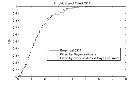
Figure 1: Plot of Empirical CDF and Fitted CDF for diabetic retinopathy data set.

Next we have tested the hypothesis that there is no significance difference between two causes of failure, i.e., we have tested the null hypothesis $H_{0}:\lambda_{1}=\lambda_{2}$ against the alternative $H_{1}:\lambda_{1}\neq\lambda_{2}$ using the method proposed in Section 5. The Bayes factor for the given data using almost non-informative prior is $2.326479\times 10^{32}$. Since the BF is very high, we conclude that two causes are not significantly different. Therefore, the conclusion from the study is that the laser treatment does not have any effect in delaying the onset of blindness to the patients with diabetic retinopathy.

Now, we consider the data without the causes of failure and fitted the data assuming Weibull distribution with shape parameter $\alpha^{*}$ and scale parameter $\lambda^{*}$. Assuming almost non-informative gamma prior for both $\alpha^{*}$ and $\lambda^{*}$, the Bayes estimates of $\alpha^{*}$ and $\lambda^{*}$ are respectively $1.5358$ and $0.4795$. The KS distance and p-value of the fit are respectively $0.0582$ and $0.9581$, which indicates the good fit of the data. The empirical and the fitted CDF of the data assuming Weibull distribution is presented in Figure 2. This can be used to estimate $E(T)$, i.e. the expected time to the onset of blindness, or to estimate $E(T|T>a)$, for some $a>0$, etc.

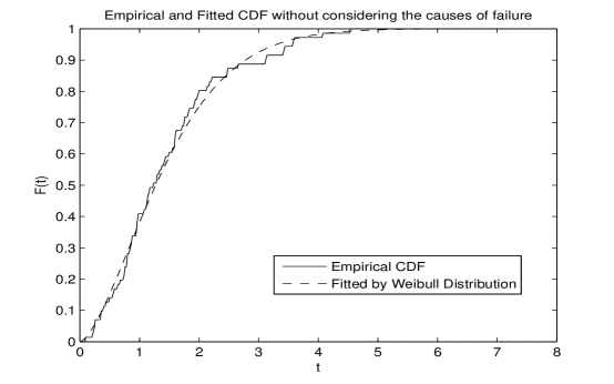
Figure 2: Plot of Empirical CDF and Fitted CDF assuming equality of two causes of failure.

7 Simulation

In this section we provide an extensive simulation study based on complete sample to verify how the proposed estimators behave for different sample sizes and for different set of parameters. Simulation results are provided for both, without order restriction and with order restriction on scale parameters. We consider three sets of parameter values of $(\alpha,\,\lambda_{0},\,\lambda_{1},\,\lambda_{2})$: Set I $(2.0,0.5,1.0,1.2)$, Set II $(2.0,1.0,1.0,1.2)$ and Set III $(2.0,1.5,1.0,1.2)$. We have taken $n$ = 30, 40, 50. We have considered almost non-informative proper priors, as suggested by Congdon (2003); the hyper parameters are $a=b=c_{1}=c_{2}=0.001$ and $a_{0}=a_{1}=a_{2}=1$. We provide the average estimates (AEs) along with the mean square errors (MSEs) of the model parameters. The average lengths (AL) and coverage percentages (CP) of $95\%$ symmetric and highest posterior density (HPD) credible intervals are also provided. All the simulation results are provided from Table 4 to Table 9 and the results are based on 5000 replications.

Some of the points are very clear from the simulation experiments. Both biases and MSEs are decreases with the increase of sample size $n$ and hence it indicates the consistency of the estimator. If we observe the ALs and CPs of different credible intervals, in all the cases CPs are closed to the nominal values and ALs are decreases with the increase of $n$. Now if we compare the inference based on partially order restriction on scale parameters with unrestricted inference then it has been observed that order restricted inference provides lower MSEs for $\lambda_{1}$ and $\lambda_{2}$ than unrestricted inference. Also the ALs of different CRIs of $\lambda_{1}$ and $\lambda_{2}$ under order restricted inference is is lower than that of unrestricted inference.

Table 4: Without order restricted Bayes estimates along with the corresponding mean square errors ($\alpha=2.0$, $\lambda_{1}=1.0$, $\lambda_{2}=1.2$).

		$\alpha$		$\lambda_{0}$		$\lambda_{1}$		$\lambda_{2}$
n	$\lambda_{0}$	AE	MSE	AE	MSE	AE	MSE	AE	MSE
30	0.5	2.035	0.091	0.569	0.062	1.050	0.120	1.232	0.150
40	0.5	2.027	0.067	0.546	0.039	1.033	0.083	1.226	0.101
50	0.5	2.013	0.053	0.538	0.032	1.034	0.068	1.214	0.079
30	1.0	2.031	0.091	1.071	0.156	1.074	0.162	1.270	0.194
40	1.0	2.023	0.067	1.054	0.108	1.058	0.105	1.241	0.131
50	1.0	2.018	0.052	1.047	0.085	1.042	0.081	1.240	0.101
30	1.5	2.036	0.091	1.608	0.375	1.108	0.215	1.316	0.256
40	1.5	2.019	0.066	1.562	0.212	1.077	0.139	1.271	0.167
50	1.5	2.015	0.050	1.546	0.156	1.056	0.094	1.254	0.118

Table 5: Order restricted Bayes estimates along with the corresponding mean square errors ($\alpha=2.0$, $\lambda_{1}=1.0$, $\lambda_{2}=1.2$).

		$\alpha$		$\lambda_{0}$		$\lambda_{1}$		$\lambda_{2}$
n	$\lambda_{0}$	AE	MSE	AE	MSE	AE	MSE	AE	MSE
30	0.5	2.041	0.095	0.570	0.062	0.939	0.066	1.352	0.147
40	0.5	2.033	0.069	0.545	0.041	0.949	0.046	1.317	0.097
50	0.5	2.016	0.052	0.537	0.033	0.952	0.036	1.286	0.065
30	1.0	2.041	0.096	1.081	0.166	0.950	0.084	1.406	0.204
40	1.0	2.024	0.068	1.051	0.107	0.959	0.063	1.360	0.135
50	1.0	2.022	0.055	1.039	0.081	0.959	0.045	1.321	0.091
30	1.5	2.040	0.096	1.615	0.350	0.964	0.114	1.453	0.289
40	1.5	2.027	0.069	1.567	0.216	0.957	0.071	1.383	0.163
50	1.5	2.015	0.052	1.552	0.168	0.960	0.055	1.346	0.115

Table 6: Coverage percentage and average length of $95\%$ symmetric CRIs (Without order restricted, $\alpha=2.0$, $\lambda_{1}=1.0$, $\lambda_{2}=1.2$).

		$\alpha$		$\lambda_{0}$		$\lambda_{1}$		$\lambda_{2}$
n	$\lambda_{0}$	AL	CP	ALL	CP	AL	CP	AL	CP
30	0.5	1.441	98.54	0.920	95.72	1.331	96.08	1.472	95.78
40	0.5	1.257	98.68	0.777	96.30	1.133	95.70	1.259	95.70
50	0.5	1.124	98.62	0.691	95.18	1.013	95.38	1.116	95.84
30	1.0	1.437	98.38	1.518	95.96	1.522	96.10	1.695	96.18
40	1.0	1.253	98.30	1.290	95.92	1.294	96.64	1.433	95.98
50	1.0	1.128	98.74	1.149	96.00	1.145	96.16	1.278	95.98
30	1.5	1.442	98.34	2.231	96.08	1.733	96.02	1.941	96.50
40	1.5	1.250	98.70	1.850	96.12	1.447	96.36	1.612	96.28
50	1.5	1.126	98.76	1.631	96.84	1.270	96.62	1.420	96.58

Table 7: Coverage percentage and average length of $95\%$ HPD CRIs (Without order restricted, $\alpha=2.0$, $\lambda_{1}=1.0$, $\lambda_{2}=1.2$).

		$\alpha$		$\lambda_{0}$		$\lambda_{1}$		$\lambda_{2}$
n	$\lambda_{0}$	AL	CP	ALL	CP	AL	CP	AL	CP
30	0.5	1.434	98.48	0.871	94.96	1.284	95.12	1.423	94.68
40	0.5	1.251	98.64	0.745	95.50	1.103	94.86	1.228	95.00
50	0.5	1.121	98.58	0.668	94.88	0.991	94.96	1.093	94.84
30	1.0	1.430	98.46	1.449	95.02	1.453	95.14	1.624	95.38
40	1.0	1.248	98.26	1.246	95.60	1.249	96.02	1.387	95.22
50	1.0	1.124	98.76	1.116	95.72	1.113	95.58	1.245	95.72
30	1.5	1.435	98.28	2.124	95.80	1.636	95.40	1.841	95.48
40	1.5	1.245	98.72	1.785	95.62	1.387	95.48	1.549	95.68
50	1.5	1.122	98.74	1.584	95.82	1.227	96.10	1.375	96.26

Table 8: Coverage percentage and average length of $95\%$ symmetric CRIs (Order restricted, $\alpha=2.0$, $\lambda_{1}=1.0$, $\lambda_{2}=1.2$).

		$\alpha$		$\lambda_{0}$		$\lambda_{1}$		$\lambda_{2}$
n	$\lambda_{0}$	AL	CP	ALL	CP	AL	CP	AL	CP
30	0.5	1.445	98.14	0.886	94.24	1.024	93.94	1.388	97.22
40	0.5	1.261	98.12	0.744	94.56	0.885	95.12	1.162	97.22
50	0.5	1.126	98.76	0.658	93.88	0.787	95.26	1.011	97.34
30	1.0	1.447	98.44	1.496	95.16	1.174	94.50	1.628	97.22
40	1.0	1.253	98.04	1.255	95.56	1.013	95.44	1.354	96.72
50	1.0	1.130	98.44	1.105	95.66	0.899	95.74	1.172	97.42
30	1.5	1.445	98.32	2.190	95.94	1.323	95.04	1.863	97.08
40	1.5	1.256	98.26	1.814	95.76	1.118	95.56	1.516	97.32
50	1.5	1.125	98.62	1.598	95.60	0.996	96.04	1.318	97.72

Table 9: Coverage percentage and average length of $95\%$ HPD CRIs (Partially Order restricted, $\alpha=2.0$, $\lambda_{1}=1.0$, $\lambda_{2}=1.2$).

		$\alpha$		$\lambda_{0}$		$\lambda_{1}$		$\lambda_{2}$
n	$\lambda_{0}$	AL	CP	ALL	CP	AL	CP	AL	CP
30	0.5	1.433	98.02	0.834	93.56	0.984	91.54	1.338	97.70
40	0.5	1.251	98.20	0.709	93.98	0.856	92.80	1.128	97.60
50	0.5	1.118	98.78	0.631	93.20	0.766	93.04	0.984	97.58
30	1.0	1.434	98.34	1.415	94.24	1.117	91.58	1.557	98.18
40	1.0	1.243	97.94	1.201	94.56	0.974	93.34	1.305	98.16
50	1.0	1.122	98.30	1.065	94.80	0.869	93.48	1.136	98.08
30	1.5	1.433	98.36	2.069	94.72	1.246	92.22	1.767	98.50
40	1.5	1.246	98.30	1.735	94.90	1.066	93.02	1.455	98.24
50	1.5	1.117	98.62	1.540	95.04	0.957	93.72	1.272	98.16

8 Conclusion

In this article we have provided the Bayesian inference of a dependent competing risk model. We assume Marshall-Olkin bivariate Weibull distribution to explain the dependency structure between two causes of failure. Bayesian inference has been provided under two scenario, in one case we assume order restriction between two causes of failures and in other case we do not assume any order restriction. We have also shown that the inference procedure for both the cases can easily be extended to different censoring schemes. We propose to use Bayes factor to test the hypothesis that there is no significant difference between two causes of failure. An extensive simulation results and a data analysis shows that the proposed method works quite well. If it is known apriori that one cause of failure is higher risk than the other then it is better to use the order restricted inference.

Appendix

Proof of Theorem 1:

$$\begin{array}[]{lll}\ln(\widetilde{\pi_{1}}(\alpha))&=&-c_{1}\alpha+(n+c_{2}-1)\ln(\alpha)-(a+n)\ln(b+\sum_{i=1}^{n}t_{i:n}^{\alpha})+(\alpha-1)\sum_{i=1}^{n}\ln(t_{i:n}),\\ \frac{\partial^{2}\ln(\widetilde{\pi_{1}}(\alpha))}{\partial\alpha^{2}}&=&-\frac{n+c_{2}-1}{\alpha^{2}}-(a+n)\bigg{[}\frac{b\sum_{i=1}^{n}t_{i:n}^{\alpha}(\ln(t_{i:n}))^{2}+\sum_{i=1}^{n}t_{i:n}^{\alpha}\sum_{i=1}^{n}t_{i:n}^{\alpha}(\ln(t_{i:n}))^{2}-(\sum_{i=1}^{n}t_{i:n}^{\alpha}\ln(t_{i:n}))^{2}}{(b+\sum_{i=1}^{n}t_{i:n}^{\alpha})^{2}}\bigg{]}\\ {}&\leq&0.\end{array}$$

Since, $\sum_{i=1}^{n}t_{i:n}^{\alpha}\sum_{i=1}^{n}t_{i:n}^{\alpha}(\ln(t_{i:n}))^{2}-(\sum_{i=1}^{n}t_{i:n}^{\alpha}\ln(t_{i:n}))^{2}\geq 0$ (by Cauchy-Schwarz inequality).

References

• [1] Balakrishnan, N., Beutner, E. and Kateri, M. (2009), “Order restricted inference for exponential step-stress models”, IEEE Transactions on Reliability, vol. 58, 132–142.
• [2] Congdon, P. (2003), Applied Bayesian Modeling, John Wiley and Sons, New York.
• [3] Cox D. R. (1959), “The analysis of exponentially distributed lifetimes with two types of failures”, Journal of the Royal Statistical Society Series B, vol. 21, 411 - 421.
• [4] Crowder M. (2001), Classical Competing Risks Model, Chapman & Hall, New York.
• [5] Devroye, L. (1884) “A simple algorithm for generating random variables with log-concave density”, Computing, vol. 33, 247–257.
• [6] , Dey, A.K and Kundu, D. (2009), “Estimating the parameters of the Marshall-Olkin bivariate Weibull distribution by EM algorithm”, Computational Statistics and Data Analysis, vol. 53, 956–965.
• [7] Feizjavdian, S.H. and Hashemi, R. (2015), Analysis of dependent competing risks in presence of progressive hybrid censoring using Marshall-Olkin bivariate Weibull distribution”, Computational Statistics and Data Analysis, vol. 82, 19–34.
• [8] Kundu, D. and Gupta, A.K. (2013), “Bayes estimation for the Marshall-Olkin bivariate Weibull distribution”, Computational Statistics and Data Analysis, vol. 57, 271–281.
• [9] Jose, K.K., Ristic, M.M. and Joseph, A. (2011), “Marshall-Olkin bivariate Weibull distributions and processes”, Statistical Papers, vol. 52, 789–798.
• [10] Kalbfleish, J.D. and Prentice, R.L. (1980), The Statistical Analysis of the Failure Time Data, Wiley, New York.
• [11] Kinderman, A.J. and Monahan, F.J. (1977) “Computer generation of random variables using the ratio of uniform deviates”, ACM Trans. Math. Software, vol. 3, 257–260.
• [12] Kundu, D. (2004), “Parameter estimation of the partially complete time and type of failure data”, Biometrical Journal, vol. 46, 165–179.
• [13] Kundu, D. and Pradhan, B. (2011), “Bayesian analysis of progressively censored competing risk data”, Sankhya, Ser. B, vol. 73, 276–296.
• [14] Lawless, J.F. (1982), Statistical Models and Methods for Lifetime Data, Wiley, New York.
• [15] Lu, J-C. (1989), “Weibull extension of the Freund and Marshall-Olkin bivariate exponential model”, IEEE Transactions on Reliability, vol. 38, 615–619.
• [16] Marshall, A.W. and Olkin, I. (1967), “A multivariate exponential distribution”, Journal of the American Statistical Association, vol. 62, 30 – 44.
• [17] Mondal, S. and Kundu, D. (2020), “Bayesian inference for Weibull distribution under the balanced joint Type-II progressive censoring scheme”, American Journal of Mathematical and Management Sciences, vol. 39, 56–74.
• [18] Pena, A. and Gupta, A.K. (1990), “Bayes estimation for the Marshall-Olkin exponential distribution”, Journal of the Royal Statistical Society , Ser B, vol. 52, 379-389.
• [19] Prentice, R. L., Kalbfleish, J. D., Peterson, Jr. A. V., Flurnoy, N., Farewell, V. T., Breslow, N. E. (1978), “The analysis of failure times in presence of competing risks”, Biometrics, vol. 34, 541 - 554.
• [20] Samanta, D. and Kundu, D. (2018), “Order restricted inference of a multiple step-stress model”, Computational Statistics and Data Analysis, vol. 117, 62–75.
• [21] Shen, Y. and Xu, A. (2018), “On the dependent competing risks using Marshall–Olkin bivariate Weibull model: Parameter estimation with different methods”, Communication in Statistics - Theory and Methods, vol. 47, 5558–5572.
• [22] Tsiatis, A. (1975), “A nonidentifiability aspect of the problem of competing risks”, Proceedings of the National Academy of Sciences, USA, vol. 72, 20-22.
• [23] Wang, C.P. and Ghosh, M. (2003), “Bayesianan alysis of bivariate competing risks models with covariates”, Journal of Statistical Planning and Inference, vol. 115, 441–459.
• [24] Xu, A. and Zhou, S. (2017), “Bayesian analysis of series system with dependent causes of failure”, Statistical Theory and Related Fields, vol. 1, 128–140.