Autoregressive Hidden Markov Models with partial knowledge on latent space applied to aero-engines prognostics

Abstract

[This paper was initially published in PHME conference in 2016, selected for further publication in International Journal of Prognostics and Health Management.]

This paper describes an Autoregressive Partially-hidden Markov model (ARPHMM) for fault detection and prognostics of equipments based on sensors’ data. It is a particular dynamic Bayesian network that allows to represent the dynamics of a system by means of a Hidden Markov Model (HMM) and an autoregressive (AR) process. The Markov chain assumes that the system is switching back and forth between internal states while the AR process ensures a temporal coherence on sensor measurements. A sound learning procedure of standard ARHMM based on maximum likelihood allows to iteratively estimate all parameters simultaneously. This paper suggests a modification of the learning procedure considering that one may have prior knowledge about the structure which becomes partially hidden. The integration of the prior is based on the Theory of Weighted Distributions which is compatible with the Expectation-Maximization algorithm in the sense that the convergence properties are still satisfied. We show how to apply this model to estimate the remaining useful life based on health indicators. The autoregressive parameters can indeed be used for prediction while the latent structure can be used to get information about the degradation level. The interest of the proposed method for prognostics and health assessment is demonstrated on CMAPSS datasets.

Keywords Prognostics  $\cdot$ Switching Markov-model  $\cdot$ Autoregressive hidden Markov model  $\cdot$ Soft labels

1 AR-Markov modelling for prognostics

Autoregressive (AR) models have been shown to be appropriate for time-series modelling in various fields such as econometric [1] and climate forecasting [2]. In condition monitoring, it is generally used for fault detection by establishing an AR model using healthy conditions under various loads and using this model on the observed data recorded in in-service conditions in order to trend the residual signals. Such approaches does not make use of analytical description of faults or collection of typical fault patterns [3, 4]. Such a method has been used for gear monitoring by [5], and [6] used a similar approach together with a logit model to determine the probability of failure of an elevator door motion system. [7] suggested to use a pole representation of an AR process to detect bearings faults. [8] compared ARIMA (AR with integrated moving average) with two other models for battery prognostics.

In structural safety, AR models were used by [9, 10] to identify structural dynamic characteristics of system subjected to ambient excitations. [11] suggested to use an ARMA to characterize and reconstruct fatigue loads for prognostics application on mechanical components. The authors proposed to adapt the parameters of this model by Bayesian updating to accommodate variability in loading and data sparsity.

[12] were interested in the modelling of switching autoregressive dynamics from multivariate vital sign time series in order to stratify mortality risks of intensive care units patients receiving particular treatments. In this biomedical application, the authors made use of a combination of an AR process and a Hidden Markov Model (HMM) called ARHMM. Such a model is able to cope with multistate non-stationary systems which are generally encountered in PHM applications.

ARHMM were also used for wind turbine monitoring by [13] where the authors were interested in the statistical representation of wind time series. They made use of a hidden Markov chain which represents the weather types and allows to switch between several autoregressive models that describe the time evolution of the wind speed. Such switching models are particular well suited for PHM applications to represent the dynamical behavior of complex systems [14, 15].

Initially proposed for speech recognition [16], an ARHMM is a particular dynamic Bayesian network that draws benefits of an AR model and HMM. A standard and sound learning procedure of this model based on maximum likelihood (ML) allows parameters to be estimated iteratively and simultaneously. This paper suggests to use ARHMM for fault detection and prognostics of equipments based on sensors’ data. A modification of the learning procedure is also proposed to enable one to add prior knowledge on the latent structure. This modification allows, in some way, to decrease the attachment of the model to the data that can be observed in practice in various probabilistic models learned with the ML approach.

Following previous work on the integration of prior on latent variables for fault detection [17, 18, 19, 20], the objective is to enable the users of probabilistic models to represent two kinds of knowledge [21, 22]:

• Generic knowledge about the data generating process and corresponding to random uncertainty. It pertains to a population of observables such as historical facts, laws of physics, statistical and common sense knowledge.

• Specific knowledge, also called relative knowledge or factual evidence, is about a given realization of the data. It pertains to a particular situation and is related to a domain or a discipline.

Specific knowledge is of key importance for PHM applications. It is not necessarily related to statistics and is generally partial because the observation process is imperfect due to lack of knowledge. It generally aims at improving skills of a method trained by generic knowledge.

The integration of the prior suggested in this paper for ARHMM is based on the Theory of Weighted Distributions (TWD) [23] which is compatible with the Expectation-Maximization (EM) algorithm in the sense that the convergence properties are still satisfied. It makes use of concepts initially developed by [17, 22] based on Dempster-Shafer’s theory of belief functions and of [24] using the TWD to include prior in EM-based learning procedures.

The resulting model is called Autoregressive Partially-Hidden Markov Model (ARPHMM) and is described in the next section. It is then shown to be well suited for remaining useful life (RUL) based on health indicators with an illlustration on CMAPSS datasets [25, 26].

2 Markov switching model with soft prior: General formulation

A measurement at time $t$, $\boldsymbol{x}_{t}$ is mathematically represented as a weighted sum of the previous measurements plus an error term, where the weights are defined conditionally to each state:

$$\boldsymbol{x}_{t}=-\sum_{\delta=1}^{\Delta}\boldsymbol{r}_{\delta}(y_{t})\boldsymbol{x}_{t-\delta}+\boldsymbol{\varepsilon}_{t}(y_{t}),\>\>1\leq t\leq T$$ (1)

The noise term

$$\boldsymbol{\varepsilon}_{t}(y_{t})\sim N(0,\boldsymbol{\Sigma}_{y_{t}})$$

is assumed to be a Gaussian with zero mean and a covariance matrix $\boldsymbol{\Sigma}_{y_{t}}$ automatically adjusted for each hidden state given the data in the learning phase. The AR coefficients for the $i$-th state are denoted as $\boldsymbol{r}_{\delta}(y_{t}=i)$ where $\delta=1\dots\Delta$ is the time lag. The set of AR coefficients is given by:

$$\mathbf{B}_{i}=\Big{(}\boldsymbol{r}_{1}(i),\dots,\boldsymbol{r}_{\delta}(i),\dots,\boldsymbol{r}_{\Delta}(i)\Big{)}\\$$ (2)

The switching between internal states is governed by a stochastic process taking the form of a Markov chain and depicted in Figure 1. It is represented by a transition matrix A with elements $a_{ij}=p(y_{t}=j|y_{t-1}=i)$ (probability of going into state $j$ at time $t$ given the state was $i$ at $t-1$). The prior probability of the chain is denoted as $\boldsymbol{\Pi}=[\pi_{1}\dots\pi_{K}]$, where $\pi_{i}$ is the probability to be in state $i$ at time $t=1$.

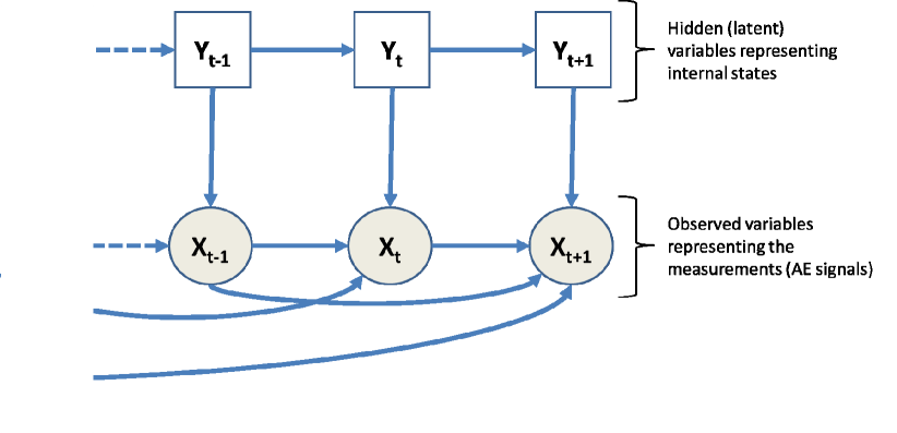
Figure 1: Graphical model of an ARHMM: Rounded boxes $\boldsymbol{X}_{t}$ represent continuous observed variables (measurements such as AE signals at time $t$), rectangular-shaped boxes $\boldsymbol{Y}_{t}$ represent hidden discrete variables. The AR process is represented by the links between measurements.

2.1 Incorporating prior knowledge on latent variables

The problem is to estimate the parameters

$$\mathbf{\lambda}=(\textbf{A},\boldsymbol{\pi},\mathbf{B}_{i},{\boldsymbol{\Sigma}}_{i}),\>\>1\leq i\leq K$$ (3)

in presence of uncertain and imprecise prior information about the hidden variables.

The prior is supposed to take the form of distributions over possible internal states given AE signals and represent users’ beliefs before some evidence is taken into account. For practical use, we assume the prior to be uncertain and imprecise so that we can cover different learning paradigms: Unsupervised learning (health states $\boldsymbol{Y}$ are supposed hidden), supervised learning (states corresponds to class fully known), semi-supervised learning (combination of both previous cases) and partially-supervised learning were some health states can be known and accompanied by a confidence degree $\mathbf{W}=[\boldsymbol{w}_{1};\dots;\boldsymbol{w}_{t};\dots;\boldsymbol{w}_{T}]$, with $\boldsymbol{w}_{t}=[w_{t}(1),\dots,w_{t}(i),\dots,w_{t}(K)]$ and $w_{t}(i)\geq 0$. This is the most general case:

• When $w_{t}(i)=1$ for a given state $i$ and $w_{t}(j)=0,j\neq i$ then the supervised case is recovered;

• When $\forall t,\forall i,w_{t}(i)=0$, then the unsupervised case is recovered.

In order to estimate the parameters of an ARPHMM in a sound manner when some prior knowledge $\mathbf{W}$ about the hidden states is available, we suggest an approach using the TWD described by Patil [23] and we derive the optimal solution in terms of maximum likelihood. It follows a similar reasoning to [24, 27] and has connections with [22].

2.2 Inference and learning in ARPHMM

The parameters (Eq. 3) are optimized by an Expectation-Maximization (EM) learning procedure [28]. In the E-step, we evaluate the expectation of the hidden variables given the data; In the M-step, the auxiliary function $Q$ has to be maximized in order to ensure that the likelihood will increase at each iteration, where $Q$ (at iteration $q$) given by:

$$\begin{array}[]{rcl}Q(\mathbf{\lambda},\mathbf{\lambda}^{(q)})&=&\displaystyle\mathbb{E}_{\mathbf{\lambda}^{(q)}}[\log(L(\mathbf{\lambda};\boldsymbol{Z})|\boldsymbol{X}]\\ &=&\displaystyle\sum_{\boldsymbol{Y}}p(\boldsymbol{Y}|\boldsymbol{X},\mathbf{\lambda}^{(q)})\log L(\mathbf{\lambda};\boldsymbol{Z})\end{array}$$ (4)

with $\boldsymbol{Z}=(\boldsymbol{X},\boldsymbol{Y})$. This expression requires to express the complete-data likelihood function which, for an ARPHMM, is given by:

$$\begin{array}[]{rcl}L(\mathbf{\lambda};\boldsymbol{Z})&=&\displaystyle p(y_{1};\boldsymbol{\Pi})\bigg{(}\prod_{t=2}^{T}p(y_{t}|y_{t-1};\mathbf{A})\bigg{)}\times\\ &&\displaystyle\prod_{t=1}^{T}p(\boldsymbol{x}_{t}|y_{t};\boldsymbol{r}_{\Delta}(y_{t}),\boldsymbol{\Sigma}_{(y_{t})})\end{array}$$ (5)

Using the Theory of Weighted Distributions (WDT) and for any positive weights $\mathbf{W}$, Eq. 4 can be modified as follows:

$$\begin{array}[]{rcl}Q(\mathbf{\lambda},\mathbf{\lambda}^{(q)})&=&\displaystyle\mathbb{E}_{\mathbf{\lambda}^{(q)}}[\log L(\mathbf{\lambda};\mathbf{z})|\mathbf{x},\mathbf{w}]\\ &=&\displaystyle\frac{\sum_{\mathbf{y}}w(\mathbf{y})p(\mathbf{y}|\mathbf{x},\mathbf{\lambda}^{(q)})\log L(\mathbf{\lambda};\mathbf{z})}{\mathbb{E}_{\mathbf{\lambda}}[w(\mathbf{y})]}\end{array}$$ (6)

This adaptation of EM for the ARHMM allows one to easily incorporate prior beliefs about the hidden states in a sound manner since EM still converges thanks to the normalisation.

We can expand the expression of $Q$, derive the expression with respect to the parameters to get the parameters at iteration $q+1$ of the modified EM. For the Markov chain, we have:

$$\pi_{i}^{(q+1)} =\gamma_{1i}^{(q)}$$ (7a)

$$a_{ij}^{(q+1)} =\frac{\sum_{t=2}^{T}\xi_{t-1,t,i,j}^{(q)}}{\sum_{t=2}^{T}\sum_{l=1}^{K}\xi_{t-1,t,i,l}^{(q)}},$$ (7b)

We can show that the expression of the posterior probabilities $\gamma$ and $\xi$ can be obtained similarly to [20], using a modified forward-backward algorithm.

For the observation model, the noise covariance is given by:

$$\begin{array}[]{rcl}\displaystyle\boldsymbol{\Sigma}_{i}^{(q+1)}&=&\displaystyle\frac{1}{\sum_{t=1}^{T}\gamma_{ti}^{(q)}}\sum_{t=1}^{T}\gamma_{ti}^{(q)}\Big{[}\boldsymbol{x}_{t}+\sum_{\delta=1}^{\Delta}\boldsymbol{r}_{\delta}^{(q)}(i)\\ &&\displaystyle\boldsymbol{x}_{t-\delta}\Big{]}\Big{[}\boldsymbol{x}_{t}+\sum_{\delta=1}^{\Delta}\boldsymbol{r}_{\delta}^{(q)}(i)\boldsymbol{x}_{t-\delta}\Big{]}^{T},\end{array}$$ (8)

and the expression of the AR coefficients defined as:

$$\begin{array}[]{rcl}\mathbf{B}_{i}^{(q+1)}&=&\Big{(}\boldsymbol{r}_{1}^{(q+1)}(i),\dots,\boldsymbol{r}_{\delta}^{(q+1)}(i),\dots,\boldsymbol{r}_{\Delta}^{(q+1)}(i)\Big{)}\\ &=&-\displaystyle\Big{[}\sum_{t=1}^{T}\gamma_{ti}^{(q)}\boldsymbol{x}_{t}\boldsymbol{u}_{t-1}^{T}\Big{]}\Big{[}\sum_{t=1}^{T}\gamma_{ti}^{(q)}\boldsymbol{u}_{t-1}\boldsymbol{u}_{t-1}^{T}\Big{]}\end{array}$$ (9)

with

$$\boldsymbol{u}_{t-1}=\Big{(}\boldsymbol{x}_{t-1},\boldsymbol{x}_{t-2},...,\boldsymbol{x}_{t-\Delta}\Big{)}^{T},$$ (10)

where the likelihood $b_{i}(\boldsymbol{x}_{t})$ given the hidden state $i$ is given by:

$$b_{i}(\boldsymbol{x}_{t})=\mathcal{N}(\boldsymbol{x}_{t}+\sum_{\delta=1}^{\Delta}\boldsymbol{r}_{\delta}(i)\boldsymbol{x}_{t-\delta}\;|\;0,\boldsymbol{\Sigma}_{i})$$ (11)

The forward pass is useful to evaluate the likelihood of the model. It is also of particular interest since it may be defined with respect to the prior on the latent structure:

$$\alpha_{1i}^{(q)} =\pi_{i}^{(q)}\;w_{1i}\;b_{i}(\boldsymbol{x}_{1}),$$ (12a)

$$\alpha_{t,j}^{(q)} =b_{j}(\boldsymbol{x}_{t})\;\underbrace{w_{tj}}_{prior}\;\sum_{i}\alpha_{t-1,i}^{(q)}\;a_{ij}^{(q)}$$ (12b)

and the likelihood of the observed data given the model is computed as:

$$L(\mathbf{\lambda}^{(q)};\boldsymbol{X},\mathbf{W})=\sum_{i=1}^{K}\alpha_{Ti}$$ (13)

2.3 ARPHMM for health assessment and prognostics

Health assessment can be performed by inferring the hidden state at the current time $t$. As in standard HMM, it is made possible by either a forward or a forward-backward passes or applying the Viterbi algorithm. The specificity of the proposed approach is to be able to exploit prior on the latent structure.

The remaining useful life can be estimated by a direct propagation computed, for instance, by a similarity-based approach. The principle is to look for a training instance in the historical data that is similar to the currently observed data and to consider that the latter would evolve in the same way [29]. The computation of the similarity is however of key importance [29, 27].

Likelihood-based approaches does not always generalize well to unobserved (quite different) cases. This could be a limitation for health assessment and prognostics on real systems. Bayesian approaches have been used for tackling such problems in PHM, mostly during the prediction phase or for RUL estimation (for instance to update noise characteristics) and specifically to integrate prior on models’ parameters [30, 31].

The Theory of Weighted Distributions used in this paper plays a similar role to the Bayesian approach but specifically on the latent variables. Its interest holds particularly in the possibility to be used in MLE-based learning which represents a learning paradigm that is widely used in PHM-related publications. The use of prior on latent variables’ configuration allows to condition some areas of the feature space which is expected to make those ML-based models more specific.

Practically, the ARPHMM can be used for health assessment and prognostics as follows:

• Learning for prognostics: Build an ARPHMM by considering the RUL as output in the AR process. Consider various parameterizations of the prior ($w$) if the internal states have no meaning. The learning procedure thus estimates the mapping between the RUL and the data conditioned on the prior.

• Health assessment on testing data: Apply the forward-backward propagations and find the most probable state, or the Viterbi algorithm. If no prior is available during inference, then $w_{t,i}=1$. If some prior information are available, then it can be used in the propagations (Eq. 12b).

• RUL estimation: For the testing phase, find the likeliest model by applying the forward pass together with either the prior used for training (by assuming that the initial wear of both training and testing data are similar) or an external prior if available. Then deduce the RUL by merging the closest instances.

Note that RUL estimation could also be performed by sampling the underlying state-space model (Eq. 1) which is not studied in this paper and let for future work.

3 Illustration on turbofan datasets

3.1 Datasets description

The turbofan datasets were generated using the CMAPSS simulation environment that represents an engine model of the 90,000 lb thrust class [25, 26]. The authors used a number of editable input parameters to specify operational profile, closed-loop controllers, environmental conditions. Some efficiency parameters were modified to simulate various degradations in different sections of the engine system. Selected fault injection parameters were varied to simulate continuous degradation trends.

The datasets generated possess unique characteristics that make them very useful and suitable for developing classification and prognostics algorithms: Multi-dimensional response from a complex non-linear system, high levels of noise, effects of faults and operational conditions, and plenty of units simulated with high variability. Benchmarking of prognostics algorithms on those datasets has been proposed and discussed in [32].

Figure 2 (taken from [27]) depicts one of the sensor measurements from a healthy situation to failure, as well as the evolution of those values in each of the six operating conditions (for instance landing, take-off, cruse and so on).

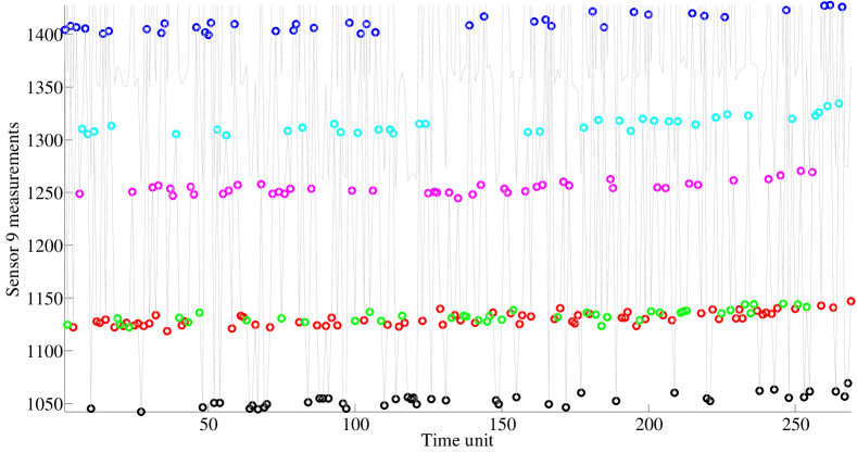
Figure 2: Operating conditions in each regime: Sensor measurements are locally linear .

Figure 3 illustrates the health indicators (computed as suggested [27] and inspired from [33]) for all training data in each dataset. Dataset $\#1$ is made of $100$ training instances with an unique operating condition (OC) and unique fault mode, dataset $\#2$ with $260$ training instances, six OCs and one fault mode, dataset $\#3$ with $100$ training instances, one OC and two fault modes, and dataset $\#4$ with $248$ training instances made of six OCs and two fault modes.

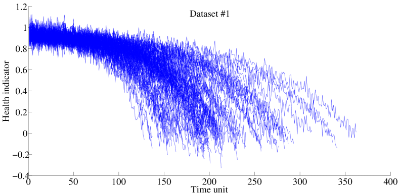
(a) #1

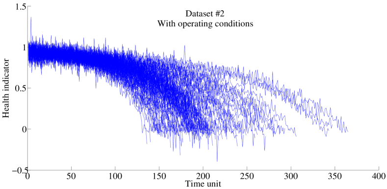
(b) #2 with operating conditions

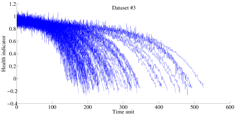
(c) #3

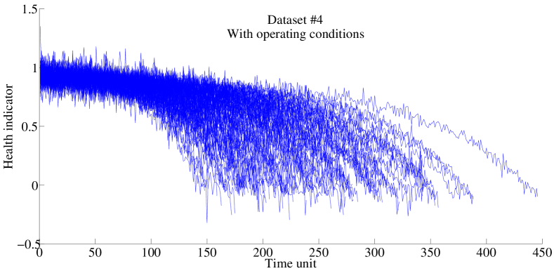
(d) #4 with operating conditions

Figure 3: Evolution of the health indices for all engines in the four datasets.

In the present paper, the $100$ training instances of the turbofan dataset $\#1$ were used for learning and the first $15$ testing for testing and comparison is made with RULCLIPPER algorithm [27] (available at the following web page: https://github.com/emmanuelramasso, with the ensemble-approach described in Table 7 of the latter publication). It is also compared to the Summation Wavelet Extreme Learning Machine (SWELM) algorithm proposed in [34].

3.2 Prior information on the latent variables of the ARPHMM

The ARPHMMs were trained using the health indicators shown in Figure 3(a) (and available at the aforementionned web page) as inputs and using the associated RUL as output. The real internal states of the turbofan are unknown but we insert some prior about some macroscopic latent variables by considering artificial finite degradation levels described in [35] (also available on the web page). Those levels, estimated by this method, are illustrated in Figure 4 for the $100$ training data.

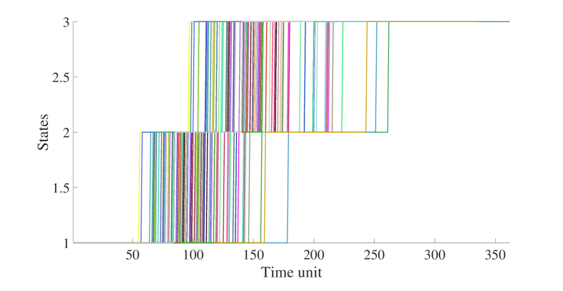
Figure 4: Evolution of the finite levels of degradation.

The number of states for each training instance was thus equal to the number of states provided by the artificial degradation levels (3), and the number of regressors was equal to $7$ for all instances (about a quarter of the shorter testing instance). Note that the optimization of those parameters requires to develop some objective criteria with respect to the prior on latent variables which will be performed in future work.

The comparison between the estimated RUL and the ground truth provided at NASA PCOE was made using the timeliness function as described in [26] and with the mean average percentage error (MAPE) which is possible since the RULs are available for dataset $\#1$.

Table 1: Results of ARPHMM and comparison. The timeliness S and the MAPE should be minimized.

Testing	Critical	True	ARPHMM			SWELM			RULCLIPPER
instance	time	RUL	proposed			[34]			[27]
			$\hat{\textrm{RUL}}$	S	MAE	$\hat{\textrm{RUL}}$	S	MAE	$\hat{\textrm{RUL}}$	S	MAE
1	31	112	115.61	0.435	3.222	112	0	0	121.95	1.705	8.884
2	49	98	107.00	1.460	9.184	54	28.507	44.898	108.03	1.727	10.236
3	126	69	78.09	1.481	13.170	68	0.08	1.449	57.960	1.338	15.998
4	106	82	79.85	0.180	2.619	80	0.166	2.439	76.832	0.488	6.302
5	98	91	87.85	0.274	3.459	100	1.459	9.890	78.119	1.693	14.155
6	105	93	80.85	1.546	13.062	108	3.482	16.129	102.173	1.502	9.863
7	160	91	78.17	1.682	14.095	114	8.974	25.274	97.015	0.824	6.605
8	166	95	75.226	3.577	20.815	102	1.014	7.368	95.886	0.093	0.933
9	55	111	108.58	0.205	2.180	105	0.587	5.405	117.586	0.932	5.933
10	192	96	73.80	4.514	23.121	68	7.618	29.167	87.219	0.965	9.146
11	83	97	95.11	0.156	1.945	67	9.051	30.928	104.005	1.015	7.222
12	217	124	85.93	17.692	30.700	131	1.014	5.645	100.939	4.894	18.598
13	195	95	83.42	1.438	12.192	92	0.259	3.158	84.444	1.252	11.112
14	46	107	112.62	0.755	5.255	81	6.389	24.299	119.931	2.644	12.085
15	76	83	89.56	0.928	7.910	106	8.974	27.711	94.711	2.225	14.109
Overall performance			-	36.32	10.86%	-	77.57	15.58%	-	23.30	10.08%
			FUSION
			S=21.8			MAPE=9.26%

Results are gathered in Table 1. Compared to RULCLIPPER, which provided the best results on dataset $\#1$ with few parameters [32], the ARPHMM provides quite similar results in term of MAPE but less in term of timeliness. This result is encouraging since no optimization was performed for the number of states nor the number of regressors. The accuracy is around $80\%$ when considering the interval $[-13,10]$ around the ground truth with a false positive rate around $67\%$ corresponding to early predictions.

ARPHMM provides better results on average compared to SWELM on those samples. However, one can observe that the fusion of elements using a simple average of RUL estimates allows to get better results than RULCLIPPER for those particular 15 instances.

The comparison can not be generalized when compared to RULCLIPPER since it has demonstrated robustness with few parameters on all turbofan datasets (with OC and two fault modes) using full testing datasets as well as on the PHM data challenge. However, the results go in favor of developing ensemble approaches made of complementary and advanced prognostics algorithms. This is all the more true than algorithms’ parameterizations play an important role on the robustness which may be criticial for in-service use.

3.3 Behavior of the proposed model

Figure 5 illustrates the use of different hidden structure for learning the evolution of the first training instance in the dataset: K=3 states without (Fig. 5(a)) and with prior (Fig. 5(b)), and K=10 states (Fig. 5(c)). The training instance and the states are then used to learn one model, which is applied on the fourth training instance of the dataset (used as a testing instance).

(a) Vacuous knowledge (only the instance is provided).

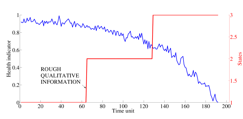
(b) Rough knowledge on states.

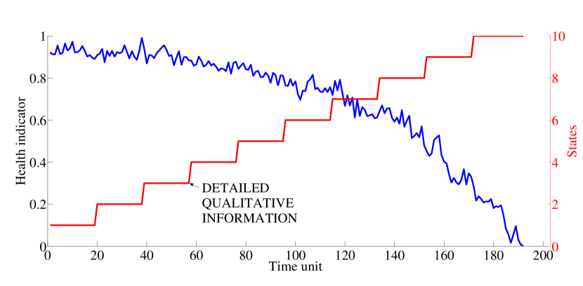
(c) Detailed knowledge on states.

Figure 5: Training instance 1, and different qualitative degradation levels used for training.

Figure 6 is the application of this model for direct RUL estimation at each time step and for the testing instance. It can be observed that the model seems to provide better results on this new instance when more states are added.

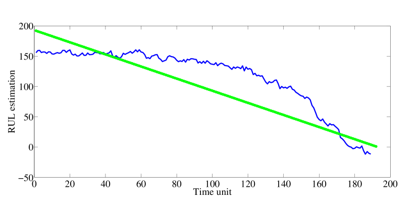
(a) RUL estimation in the vacuous case.

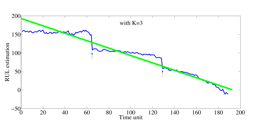
(b) RUL estimation using 3 states.

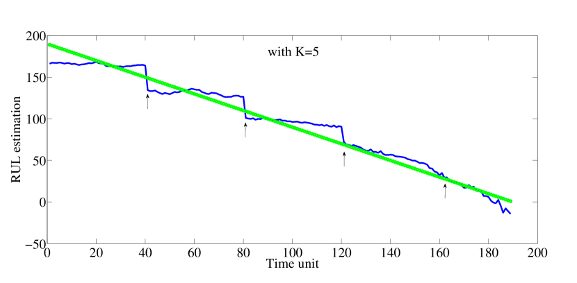
(c) RUL estimation using 5 states.

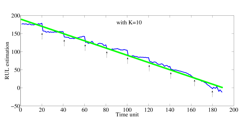
(d) RUL estimation using 10 states.

Figure 6: RUL estimation with different configurations on the hidden structure.

Finally, Figure 7 illustrates the impact of the quality of the prior. This case may correspond to a situation where new but partial knowledge is available and has to be integrated during prognostics (for instance information on the operating conditions). The quality is varied using a random sampling of the uncertainty on states as proposed in [17] (code available at the aforementionned web page). The sampling process is governed by a parameter $\rho\in[0,1]$ such that $\rho=0$ corresponds to the supervised (full quality) case, $\rho=1$ to the unsupervised case (no prior), and intermediary values correspond to noisy prior, all the more noisy than $\rho$ increases.

It can be observed that for $K=3$, the RUL estimation is highly dependent on the prior. Besides, the uncertainty can be quantified with different values of $\rho$. Uncertainty is much higher is the elbow part of the degradation, while it is quite low for the beginning (since all data have similar evolution) and for the end (when converging to the solution). For $K=10$, the RUL estimation is more accurate and does not depend on the prior.

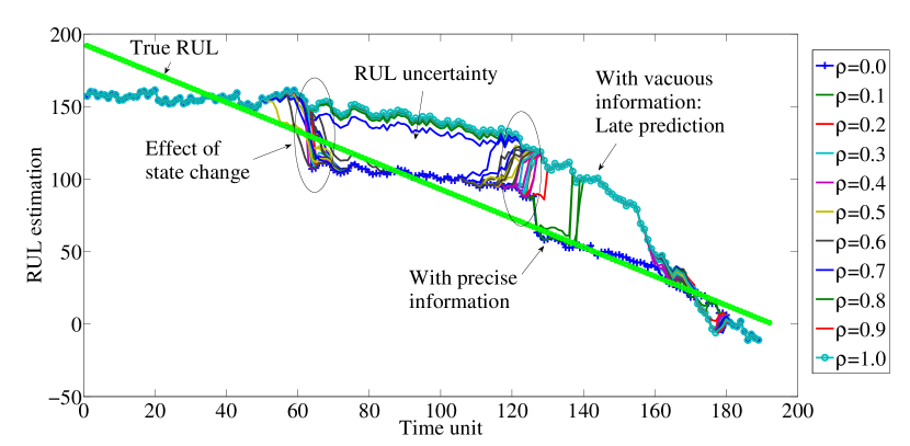
(a) K=3.

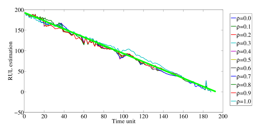
(b) K=10.

Figure 7: RUL estimation as a function of the quality of prior ($\rho$) and states

Those figures also remind prognostics approaches based on multi-modelling such as [36] and [37]. As for multimodels, the hidden structure in an ARPHMM allows to evaluate the active feature space, while, for each state, the evolution of the time-series is approximated. However, in addition to quantifying the uncertainty on states for each new measurement, the ARPHMM additionally quantifies the likelihood associated to a model which makes model selection possible.

4 Conclusion and perspectives

In this paper, we investigate the use of uncertain prior on the latent structure of dynamic Bayesian network for prognostics, and in particular an autoregressive partially hidden Markov model. More experiments are needed to validate the approach but results obtained on some instances of CMAPSS datasets are encouraging when compared to other approaches from the literature. This model is being improved to include uncertain future operating conditions on the latent structure.

References

- [1] Serena Ng and Timothy Vogelsang. Forecasting autoregressive time series in the presence of deterministic components. The Econometrics Journal, 5(1):196–224, 2002.
- [2] Hans V. Storch and Francis W. Zwiers. Statistical Analysis in Climate Research. Cambridge University Press, 1999.
- [3] Charles R. Farrar and Keith Worden. Structural Health Monitoring: A Machine Learning Perspective. John Wiley & Sons, Ltd, 2013.
- [4] Francisco Serdio, Edwin Lughofer, Kurt Pichler, Thomas Buchegger, Markus Pichler, and Hajrudin Efendic. Multivariate fault detection using vector autoregressive moving average and orthogonal transformation in residual space. In Annual Conference of the Prognostics and Health Management Society, volume 4, 2013.
- [5] Wenyi Wang and Albert K Wong. Autoregressive model-based gear fault diagnosis. Journal of vibration and acoustics, 124(2):172–179, 2002.
- [6] Jihong Yan, Muammer Koc, and Jay Lee. A prognostic algorithm for machine performance assessment and its application. Production Planning & Control, 15(8):796–801, 2004.
- [7] Suguna Thanagasundram, Sarah Spurgeon, and Fernando Soares Schlindwein. A fault detection tool using analysis from an autoregressive model pole trajectory. Journal of Sound and Vibration, 317(35):975 – 993, 2008.
- [8] Bhaskar Saha, Kai Goebel, and Jon Christophersen. Comparison of prognostic algorithms for estimating remaining useful life of batteries. In Transactions of the Institute of Measurement and Control, 2009.
- [9] Xia He and Guido De Roeck. System identification of mechanical structures by a high-order multivariate autoregressive model. Computers & structures, 64(1):341–351, 1997.
- [10] CS Huang. Structural identification from ambient vibration measurement using the multivariate ar model. Journal of Sound and Vibration, 241(3):337–359, 2001.
- [11] You Ling, Christopher Shantz, Sankaran Mahadevan, and Shankar Sankararaman. Stochastic prediction of fatigue loading using real-time monitoring data. International Journal of Fatigue, 33(7):868 – 879, 2011.
- [12] L.W.H. Lehman, S. Nemati, and R.G. Mark. Hemodynamic monitoring using switching autoregressive dynamics of multivariate vital sign time series. In Computing in Cardiology, Nice, France, 2015.
- [13] Pierre Ailliot and Valerie Monbet. Markov-switching autoregressive models for wind time series. Environmental Modelling & Software, 30:92 – 101, 2012.
- [14] L. Serir, E. Ramasso, P. Nectoux, and N. Zerhouni. E2GKpro: An evidential evolving multi-modeling approach for system behavior prediction with applications. Mechanical Systems and Signal Processing, 37(1-2):213 – 228, 2013.
- [15] Pin Lim, Chi Keong Goh, Kay Chen Tan, , and Partha Dutta. Multimodal degradation prognostics based on switching kalman filter ensemble. IEEE Trans. on Neural Networks and Learning Systems, 2016. 10.1109/TNNLS.2015.2504389.
- [16] L. Rabiner. A tutorial on hidden Markov models and selected applications in speech recognition. Proc. of the IEEE, 77(2):257–286, 1989.
- [17] E. Côme, L. Oukhellou, T. Denoeux, and P. Aknin. Learning from partially supervised data using mixture models and belief functions. Pattern recognition, 42(3):334–348, 2009.
- [18] E. Ramasso. Contribution of belief functions to hidden markov models with an application to fault diagnosis. In IEEE International Worshop on Machine Learning for Signal Processing, MLSP’09., pages 1–6, 2009.
- [19] Z. Cherfi, L. Oukhellou, E. Côme, T. Denoeux, and P. Aknin. Partially supervised independent factor analysis using soft labels elicited from multiple experts: Application to railway track circuit diagnosis. Soft Computing, 16:741–754, 2012.
- [20] E. Ramasso and T. Denoeux. Making use of partial knowledge about hidden states in HMMs: an approach based on belief functions. Fuzzy Systems, IEEE Transactions on, 22(2):395–405, 2014.
- [21] D. Dubois. Uncertainty theories: a unified view. In IEEE Cybernetic Systems Conference, pages 4–9, Dublin, Ireland, 2007.
- [22] T. Denoeux. Maximum likelihood estimation from uncertain data in the belief function framework. Knowledge and Data Engineering, IEEE Transactions on, 25(1):119–130, 2013.
- [23] G.P. Patil. Weighted distributions, volume 4. John Wiley & Sons, Ltd, Chichester, 2002. pp. 2369-2377.
- [24] P. Juesas and E. Ramasso. Ascertainment-adjusted parameter estimation approach to improve robustness against misspecification of health monitoring methods. Mechanical Systems and Signal Processing, 2016. Accepted.
- [25] D.K. Frederick, J.A. DeCastro, and J.S. Litt. User’s guide for the commercial modular aero-propulsion system simulation (C-MAPSS). Technical report, National Aeronautics and Space Administration (NASA), Glenn Research Center, Cleveland, Ohio 44135, USA, 2007.
- [26] A. Saxena, K. Goebel, D. Simon, and N. Eklund. Damage propagation modeling for aircraft engine run-to-failure simulation. In International Conference on Prognostics and Health Management, pages 1–9, Denver, CO, USA, 2008. IEEE.
- [27] E. Ramasso. Investigating computational geometry for failure prognostics. Int. Journal on Prognostics and Health Management, 5(5):1–18, 2014.
- [28] A.P. Dempster, N.M. Laird, and D.B. Rubin. Maximum likelihood from incomplete data via the EM algorithm. Journal of the Royal Statistical Society, 39(1):1–38, 1977.
- [29] T. Wang, J. Yu, D. Siegel, and J. Lee. A similarity-based prognostics approach for remaining useful life estimation of engineered systems. In Int. Conf. on Prognostics and Health Management, pages 1–6, 2008.
- [30] Bhaskar Saha and Kai Goebel. Uncertainty management for diagnostics and prognostics of batteries using bayesian techniques. In Aerospace Conference, 2008 IEEE, pages 1–8. IEEE, 2008.
- [31] Shankar Sankararaman and Kai Goebel. Uncertainty in prognostics and systems health management. Int. Journal of Prognostics and Health Management, 6:1–14, 2015.
- [32] E. Ramasso and A. Saxena. Performance benchmarking and analysis of prognostic methods for CMAPSS datasets. International Journal on Prognostics and Health Management, 5(2):1–15, 2014.
- [33] T. Wang. Trajectory Similarity Based Prediction for Remaining Useful Life Estimation. PhD thesis, University of Cincinnati, 2010.
- [34] K. Javed, R. Gouriveau, and N. Zerhouni. Novel failure prognostics approach with dynamic thresholds for machine degradation. In IEEE IECON, pages 4402–4407, Austria, 2013.
- [35] Emmanuel Ramasso. Segmentation of CMAPSS health indicators into discrete states for sequence-based classification and prediction purposes. Technical Report 6839, FEMTO-ST institute, January 2016.
- [36] L. Serir, E. Ramasso, and N. Zerhouni. An evidential evolving multimodeling approach for systems behavior prediction. In Annual Conference of the Prognostics and Health Management Society, PHM’11, Montreal, QC, Canada, 2011.
- [37] Lisa Serir, Emmanuel Ramasso, and Noureddine Zerhouni. An evidential evolving prognostic approach and its application to pronostia’s data streams. In Annual Conference of the Prognostics and Health Management Society, PHM’12, volume 3, pages 9–pages, 2012.