Adversarial Example Detection for DNN Models: A Review and Experimental Comparison

Abstract

dl has shown great success in many human-related tasks, which has led to its adoption in many computer vision based applications, such as security surveillance systems, autonomous vehicles and healthcare. Such safety-critical applications have to draw their path to success deployment once they have the capability to overcome safety-critical challenges. Among these challenges are the defense against or/and the detection of the adversarial examples. Adversaries can carefully craft small, often imperceptible, noise called perturbations to be added to the clean image to generate the AE. The aim of AE is to fool the deep learning (DL) model which makes it a potential risk for DL applications. Many test-time evasion attacks and countermeasures, i.e., defense or detection methods, are proposed in the literature. Moreover, few reviews and surveys were published and theoretically showed the taxonomy of the threats and the countermeasure methods with little focus in AE detection methods. In this paper, we focus on image classification task and attempt to provide a survey for detection methods of test-time evasion attacks on neural network classifiers. A detailed discussion for such methods is provided with experimental results for eight state-of-the-art detectors under different scenarios on four datasets. We also provide potential challenges and future perspectives for this research direction.

1 Introduction

ml, as an artificial intelligence (AI) discipline, witnessed a great success in different fields, especially in human-related tasks, such as image classification and segmentation krizhevsky2012imagenet ; simonyan2014very ; ren2015faster ; long2015fully , object detection and tracking bertinetto2016fully ; danelljan2017eco , healthcare ker2017deep , translation bahdanau2014neural and speech recognition hannun2014deep . Its high accuracy comes from continuous development of machine learning (ML) models, the availability of data and the increase in computational power. Image classification applications are constantly growing and deployed in medical imaging systems, autonomous cars, and safety-critical applications kurakin2016adversarial ; evtimov2017robust ; gu2017badnets ; papernot2017practical ; melis2017deep .

Recently and after the potential success of convolutional neural networks o2015introduction for image classification tasks, the focus of this survey, many DL models are developed, such as, for instance, VGG16 simonyan2014very ,ResNet he2016deep , InceptionV3 szegedy2016rethinking and MobileNet howard2017mobilenets . These models and others achieve high prediction accuracy on different publicly available datasets such as MNIST lecun1998gradient , CIFAR10 krizhevsky2009learning , SVHN netzer2011reading , Tiny ImageNet yao2015tiny , and ImageNet imagenet_cvpr09 . For other human tasks, many models also exist in the literature, such as R-CNN girshick2014rich , Fast R-CNN girshick2015fast and YOLO redmon2016you , which are models for object detection task, while BERT devlin2019bert , XLNet yang2020xlnet and ALBERTlan2020albert are models for natural language processing (NLP) tasks.

This DL’s bright face has been challenged by the adversaries. We can categorise the adversary’s attack into two broad categories: poisoning and evasion attacks PITROPAKIS2019100199 . In the poisoning attack, the adversary is aiming at contaminating the training data that takes place during the training time of the model. Poisoning-based backdoor attack li2020backdoor is one of the popular ways to poison the training data. While for evasion attacks, Szegedy et al. szegedy2013intriguing uncovered the potential risk facing DL models for image classification. In this paper, we review the detection methods of evasion attacks. It was shown that the adversary, in the testing time, can carefully craft small noise, called perturbation, to be added to the input of the DL model to generate the AE, as described in Figure 1. The generated AE looks perceptually like the original clean image, the perturbation is hardly perceptible for humans, while the DL model misclassifies it. The specific objective of the adversary is to: 1) have false predictions for the input samples, 2) get high confidence for the falsely predicted samples, and/or 3) possess transferability property whereby the AEs that are designed for a specific model can fool other models. The adversarial attacks threat is very challenging since the identification of AE and its features are hard to predict carlini2017adversarial ; ilyas2019adversarial . According to the available information, the adversary can generate AEs in three different scenarios including, white box, black box and gray box attacks akhtar2018threat ; hao2020adversarial . In white box attack scenario, the adversary knows everything about the DL model, including model architecture and its weights, and the model inputs and outputs. Specifically, in this setting, the AE is generated by solving an optimization problem with the guidance of the model gradients kurakin2016adversarial ; goodfellow2014explaining ; moosavi2016deepfool ; carlini2017towards ; madry2017towards . In black box scenario, the adversary has no knowledge about the model. Thus, by using the transferability property papernot2016transferability of AEs and the input samples content, the adversary can generate harmonious AE of the input sample chen2017zoo ; engstrom2019exploring ; su2019one ; kotyan2019adversarial . Finally, in the gray box scenario, the adversary has limited knowledge about the model. He has access to the training data of the model, but does not have any knowledge about the model architecture. Thus, his goal is to substitute the original model with an approximated one, then use its gradient as in white box scenario to generate AEs.

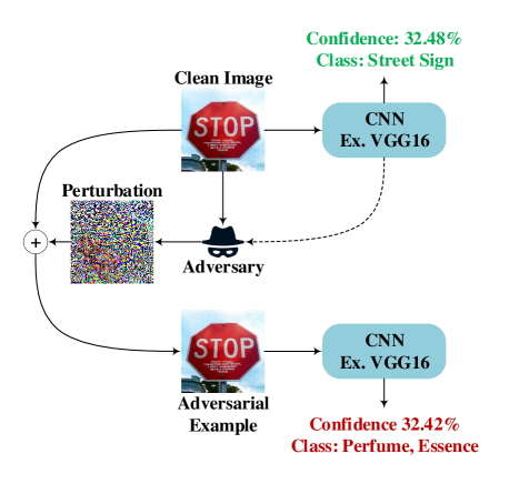
Figure 1: The overall objective of the adversary is to fool the ML model by adding an imperceptible noise to the original image to generate an adversarial image.

Adversarial attacks are not limited to image classification tasks, other machine learning tasks’ models are also vulnerable to adversarial attacks, such as object detection xie2017adversarial ; lu2017no , NLP zhang2020adversarial ; sun2020advbert ; li2019universal , speech recognition wang2020adversarial , physical world ren2021adversarial , cybersecuritydasgupta2019survey and medical imaging finlayson2018adversarial .

Since uncovering this threat to DL models, researchers put huge efforts to propose emerging methods to detect or to defend against AEs. Defense techniques like adversarial training goodfellow2014explaining ; madry2017towards ; xie2020smooth ; tramer2017ensemble , feature denoising xie2019feature ; borkar2020defending ; liao2018defense , preprocessing bakhti2019ddsa ; mustafa2019image ; prakash2018deflecting and gradient masking papernot2016distillation ; papernot2017practical ; gu2014towards ; nayebi2017biologically try to make the model robust against the attacks and let the model correctly classify the AEs. On the other hand, detecting techniques like statistical-based grosse2017statistical , denoiser-based meng2017magnet , consistency-based like feature squeezing xu2017feature , classification-based grosse2016adversarial and network invariant ma2019nic techniques try to predict/reject the input sample if it is adversarial before being passed to the DL model. Besides, the brightening face of this threat is that it makes forward steps in understanding and improving deep learning ortiz2020optimism .

In attempts to highlight the potential challenges and to organize this research direction, few surveys have been published akhtar2018threat ; hao2020adversarial ; yuan2019adversarial ; chakraborty2018adversarial . These reviews are more focusing on theoretical aspects of adversarial attacks and the countermeasures, particularly defense methods, with a lack of focus on adversarial detection techniques. Furthermore, these reviews never showed experimental comparisons between attacks and its counter-measurements. In this review paper, we give the first insight into the theoretical and experimental aspects of test-time AEs detection techniques for computer vision image classification tasks. Therefore, our key contributions can be summarized as follows:

• We provide a review for state-of-the-art AEs detection methods and categorize them with respect to the knowledge of adversarial attacks and with respect to the technique that is used to distinguish clean and adversarial inputs.

• We provide the first experimental study for state-of-the-art AEs detection methods that are tested to detect inputs crafted using different AA types, i.e., white-, black- and gray-box attacks, on four publicly available datasets, MNIST lecun1998gradient , CIFAR10 krizhevsky2009learning , SVHN netzer2011reading , and Tiny-ImageNet yao2015tiny . The summary of the experiments is shown in Figure 4.

• We provide a detailed discussion on AEs from the point of view of their content and their impact on the detection methods.

• We publicly release the testing framework that can be used to reproduce the results. The framework is scalable and new detection methods can easily be included. Moreover, a benchmark website is released to promote researchers to contribute and to publish the results of their detectors against different types of the attacks.

The rest of the paper is structured as follows. Related work is discussed in Section 2. In Section 3, a brief review of notations, definitions, threat models, adversarial attack algorithms and defense models are presented. Section 4 is dedicated to discuss the AEs detection methods in detail. Then, we present the comparison experiments and discuss in detail the results in Section 5 and Section 6, respectively. Finally, we conclude with challenges and future perspectives of this research direction in Section 7.

2 Related work

Different approaches to generate AEs in addition to countermeasures to deal with them have been proposed. Akhtar et al. akhtar2018threat published the first review covering this research field which includes works done before 2018. They classified the countermeasure methods based on where the modification is applied to the components of the model. They considered three classes as follows: 1) methods that change data, i.e., training or input data, 2) methods that change the model, and 3) methods that depend on add-on networks. Next, Yuan et al. yuan2019adversarial and Wang et al. wang2019security reviewed the defense methods and categorized them with respect to the type of action against the AEs as follows: 1) reactive methods that deal with AEs after building the DL model and 2) proactive methods that make DL models robust before generating the AEs. In their work, the authors classify the detection methods as reactive. Chakraborty et al. chakraborty2018adversarial extensively discussed the types of attacks from different points of view, but briefly discussed the defense methods including the detection methods. In hao2020adversarial , the authors were the first who classified the detection methods into: 1) auxiliary models in which a subnetwork or a separate network acts as classifier to predict adversarial inputs, 2) statistical models in which statistical analyses were used to distinguish between normal and adversarial inputs and 3) prediction consistency based models that depends on the model prediction if the input or the model parameters are changed. The review of Machado et al.machado2020adversarial treated auxiliary detection models as one taxonomy of defenses. In the review of Bulusu et al. bulusu2020anomalous and of Miller et al. miller2019not ; miller2020adversarial , they classified detection methods with respect to the presence of AEs in the training process of the detector into: 1) supervised detection in which AEs are used in the training of the detector and 2) unsupervised detection in which the detector is only trained using normal training data. Serban et al.serban2020adversarial introduced a new taxonomy of the defenses. The first category is called Guards and the second category is called defense by design. In the former, where the detection methods are categorised in, the defense method does not interact with the under attack and only builds precautions around it, while in the latter category, the defense acts directly on the model architecture and the training data. Carlini et al. carlini2017adversarial did an experimental study on ten detectors to show that all tested detectors can be broken by building new loss functions, but the work in carlini2017adversarial did not compare the detectors’ performance.

The aforementioned reviews did a great job, but detection methods are not classified and discussed in more detail, besides they are not compared to each other experimentally. In addition, considerable new detection methods have been released recently.

3 Adversarial attacks and defense methods

In this section, we briefly introduce the basic concepts of AAs that target DL models of computer vision. Firstly, the notations that are used in the literature for DL models and AAs are provided. Secondly, the threat models that DL models face are presented. Finally, the state-of-the-art attacks and defenses methods are described, excluding the adversarial detection methods that will be discussed in more detail in Section 4.

3.1 Notations and definitions

The deep neural network (DNN) and convolutional neural network (CNN) are basically a fitting function $f$ that uses its neural nodes’ interconnections to extract features from labeled raw data. Let $\mathcal{X}$ be an input space, e.g., images, and $\mathcal{Y}$ a label space, e.g., classification labels. Let $\mathbb{P}(X,Y)$ be the data distribution over $\mathcal{X}\times\mathcal{Y}$. A model $f:X\rightarrow Y$, is called a prediction function. The neural networks are trained, typically, using stochastic gradient descent (SGD) algorithm that uses the backpropagation of the error to update the model weights $\theta$. To calculate this error/loss, a loss function $\ell:Y\times Y\rightarrow\mathbb{R}^{2}$ is defined. The objective for a labeled set $S_{m}={(x_{i},y_{i})}_{i=1}^{m}\subseteq(\mathcal{X}\times\mathcal{Y})^{m}$ sampled i.i.d. from $\mathbb{P}(X,Y)$, where $m$ is the number of training samples, is to reduce the empirical risk of the prediction function $f$ is $\hat{r}(f\mid S_{m})\triangleq\frac{1}{m}\sum_{i=1}^{m}\ell(f(x_{i}),y_{i})$.

The goal of the adversary, then, given the model $f$ and input sample ($x,y$) is to find an adversarial input $x^{\prime}$, such that $||x^{\prime}-x||<\epsilon$ and $f(x)\neq f(x^{\prime})$, where $\epsilon$ is the maximum allowed perturbation and $\epsilon\in\mathcal{R}^{n}$.

Table 1 and Table 2 list respectively notations and definitions used in the literature and used in adversarial detection methods.

Table 1: List of notations.

Notation	Description
$x$	Clean input image
$y$	Clean input label
$x^{\prime}$	Adversarial example of $x$
$y^{\prime}$	Adversarial input label
$t$	Target label of adversarial attack
$f(.)$	Prediction function. It returns the probability of each class as $f(x)=softmax(z(x))$
$\theta$	Model $f$ parameters/weights
$\ell(,)$	Loss function
$\delta=x^{\prime}-x$	Perturbation, noise added to clean sample, or the difference between adversarial and clean samples
$||\delta||$	The similarity (distance) between $x$ and $x^{\prime}$
$\epsilon$	The maximum allowed perturbation
$\nabla$	Model $f$ gradient
$z$	Logits, output of the layer before $softmax$
$\sigma$	Activation function
$||.||_{p}$	$\ell_{p}$-norm

3.2 Threat models

Threat model refers to conditions under which the AEs are generated. It can be categorized according to many factors. In literature akhtar2018threat ; hao2020adversarial ; yuan2019adversarial ; chakraborty2018adversarial , adversary knowledge, adversary goal, adversary capabilities, attack frequency, adversarial falsification, adversarial specificity and attack surface are the identified factors. We focus here in threat model that is identified by adversary knowledge and adversarial specificity:

1. Adversary knowledge

   1. Adversary knowledge of baseline DL model:

      • White box attacks: the adversary knows everything about the victim model: training data, outputs and model architecture and weights. The adversary takes advantage of model information, especially the gradients, to generate the AE.

      • Black box attacks: the adversary doesn’t have access to the victim model configurations. He takes advantage of information acquired by querying and monitoring inputs and outputs of the victim model.

      • Gray box attacks: the adversary has knowledge about training data but not the model architecture. Thus, he relies on the transferability property of the AE and builds a substitute model that does the same task of the victim model to generate AE. Gray box attacks are also known as semi-white box attacks.

   2. Adversary knowledge of detection method biggio2013evasion :

      • No/Zero knowledge adversary: the adversary only knows the victim model and doesn’t know the detection technique, and he generates AE using the victim model.

      • Perfect knowledge adversary: the adversary knows that the victim model has been secured with a detection technique and he knows the configurations (architecture, training data and detection output) of the detection mode, and uses them to generate AE.

      • Limited knowledge adversary: the adversary knows the feature representation and the type of the detection technique, but doesn’t have access to the detection architecture and the training data. Hence, he estimates the detection function in order to generate the AE.

   Table 2: List of definitions.

   Definition	Description
   Adversary	Who generates the adversarial examples
   Threat model	Conditions, scenario, or environment under which that attack is performed. Such as white box attack
   Defense	Technique to make DL robust against attacks
   Detector	Technique to predict whether the input is adversarial or not
   Transferability	A property of adversarial example that shows the attack ability to fool models that aren’t used to generate it
   White box attacks	The adversary knows detailed information about the victim DL model
   Black box attacks	The adversary knows nothing about the victim DL model but he can access inputs and outputs of the model
   Gray box attacks	The adversary has limited knowledge about the victim DL model, i.e., training data
   Targeted attacks	Attacks that induce the victim DL model to classify the input sample into a specific target label $t$
   Untargeted attacks	Attacks that induce the victim DL model to classify the input sample into target label $t$ that is not equal to $y$

2. Adversarial specificity:

   1. Targeted attacks: the adversary generates the AE to misguide the DL model to classify the input sample into a specific target label $t$. The adversary generates the AE by maximizing the probability of the target label. Targeted attacks’ generation is harder than untargeted attacks’ generation due to the limited space to redirect the AE to a target label $t$. Consequently, the targeted attacks are shown to have higher perturbations than untargeted attacks and have less success rates carlini2017towards ; liu2016delving .

   2. Untargeted attacks: the adversary generates the AE to misguide the DL model to classify the input sample into a target label $t$ that is different from the correct label $y$. The adversary generates the AE by minimizing the probability of the correct label $y$. The adversary can also conduct the attack by generating multiple targeted attacks and then selects the one with minimum perturbation.

3.3 Adversarial attacks

Generally speaking, not only neural networks are vulnerable to AAs but other ML models are facing the threat as well. Many attacks and defenses were implemented for ML models, readers can refer to biggio2014pattern ; biggio2014security ; biggio2018wild for more information. In this work, we go through attacks that are targeting the image classification task of neural network szegedy2013intriguing . The main categorization of AA depends on the adversary’s knowledge about the classification model, i.e., categorised by white box and black box attacks.

3.3.1 White box attacks

L-BFGS Attack szegedy2013intriguing . limited memory broyden-fletcher-goldfarb-shanno (L-BFGS) attack is the first developed attack in the series. It aims at finding minimum perturbation $\delta$ such that $y^{\prime}=t$ and $x^{\prime}$ in the range of input domain. This optimization problem is solved approximately using box-constrained L-BFGS algorithm liu1989limited by introducing a loss function $\ell$ as follows:

$$\operatorname*{argmin}_{\delta}c\,||\delta||+\ell(x^{\prime},t),\text{ such that }x^{\prime}\in[0,1]^{n}$$ (1)

where $c$ is a regularisation parameter that we continuously search for to find minimum $\delta$ since neural networks are non-convex networks. Hence, the first term is to find minimum perturbation and the second term is to make sure that the loss value is small between $x^{\prime}$ and the target label $t$.

FGSM attack goodfellow2014explaining . It is the first developed $L_{\infty}$ attack that uses DL gradients to generate an AE. fast gradient sign method (FGSM) attack is a one-step gradient update algorithm that finds the perturbation direction, i.e., the sign of gradient, at each pixel of input $x$ that maximizes the loss value of the DL model. It is expressed as follows

$$x^{\prime}=x+\epsilon\operatorname{sign}(\nabla_{x}\ell(x,y)),\text{ such that }x^{\prime}\in[0,1]^{n}$$ (2)

where $\epsilon$ is a parameter to control the perturbation amount such that $||x^{\prime}-x||_{\infty}<\epsilon$.

BIM attack kurakin2016adversarial . It is the iterative version of the FGSM attack. basic iterative method (BIM) attack applies FGSM attack $k$ times. It is expressed as:

$$\begin{gathered}x_{i+1}^{\prime}=x_{i}^{\prime}+\alpha\operatorname{sign}(\nabla_{x}\ell(x_{i}^{\prime},y)),\\ \text{ such that }x_{0}^{\prime}=x\text{ , }x_{i+1}^{\prime}\in[0,1]^{n}\text{ , and }i=0\text{ to }k\end{gathered}$$ (3)

where $\alpha$ is the parameter to control the $i^{th}$ iteration step size and it is $0<\alpha<\epsilon$.
PGD attack madry2017towards . It is an iterative method similar to BIM attack. Unlike BIM, in order to generate “most-adversarial” example, i.e., to find local maximum loss value of the model, projected gradient descent (PGD) attack starts from a random perturbation in $L_{p}$-ball around the input sample. Many restarts might be applied in the algorithm. $L_{1}$, $L_{2}$, and $L_{\infty}$ can be used to initialize the perturbation $||x^{\prime}-x||_{p}<\epsilon$. Recently, a budget-aware step size-free variant of PGD croce2020reliable was proposed. Unlike PGD, Auto-PGD adds a momentum term to the gradient step, adapts the step size across iterations depending on the overall attack budget, and then restarts from the best point.

CW attack carlini2017towards . Carlini and Wagner followed the optimization problem of L-BFGS (see (1)) with few changes. Firstly, they replaced the loss function with an objective function

$$g(x^{\prime})=\max(\max_{i\neq t}(Z(x^{\prime})_{i})-Z(x^{\prime})_{t},-k),$$ (4)

where $Z$ is the softmax function and $k$ is the confidence parameter. The authors also provided other six objective functions carlini2017towards . Hence, the optimization problem became like

$$\underset{\delta}{\text{min}}||\delta||+c\,g(x^{\prime}),\text{ such that }x^{\prime}\in[0,1]^{n},$$ (5)

Thus, minimizing $g$ helps to find $x^{\prime}$ that has a higher score for class $t$. The authors, secondly, converted the optimization from box-constrained to unconstrained problem by introducing $w$ to control the perturbation of the input sample, such that $\delta=\frac{1}{2}(\tanh(w)+1)-x$. The carlini-wagner (CW) attack came with three variants to measure the similarity between $x^{\prime}$ and $x$ relying on $L_{0}$, $L_{2}$, and $L_{\infty}$. This attack is considered as one of the state-of-the-art attacks. It is firstly implemented to break distillation knowledge defense papernot2016distillation and it was shown it is stronger than FGSM and BIM attacks.

df attack moosavi2016deepfool . Moosavi-Dezfooli et al.introduced an attack that generates smaller perturbation than FGSM at the same fooling ratio. Given a binary affine classifier $\mathcal{F}=\{x:f(x)=0\}$, where $f(x)=w^{T}x+b$, deepFool (DF) attack defines the orthogonal projection of $x_{0}$ onto $\mathcal{F}$ as the minimal perturbation that is needed to change the classifier’s decision, and it is calculated as $\delta_{*}=-\frac{f(x)}{||w||^{2}}w$. At each iteration, DF attack solves the following optimization problem

$$\begin{gathered}\operatorname*{argmin}_{\delta_{i}}||\delta_{i}||_{2},\\ \text{ such that }f(x_{i})+\nabla f(x_{i})^{T}\delta_{i}=0\end{gathered}$$ (6)

and these perturbations are accumulated to get the final perturbation.

UAP attack moosavi2017universal . It is one of the strongest attacks that generates image-agnostic universal perturbation $v$ that can be added to any input sample and fool the DL model with up to selected fool rate $fr$. The goal is to find $v$ that satisfies the following two constraints:

$$\begin{gathered}||v||_{p}\leq\epsilon\\ \mathcal{P}(f(x+v)\neq f(x))\geq 1-fr.\end{gathered}$$ (7)

The authors used DF attack (see (6)) to calculate $v$, but any other attack algorithm can be used such as PGD or FGSM.

Other attacks. In literature, there are many other attack algorithms. Papernot et al. papernot2016limitations proposed a $L_{0}$ attack named jacobian saliency map attack (JSMA). JSMA uses DL model gradient to calculate a Jacobian based saliency map that ranks the importance of each pixel in the image. Then, JSMA modifies a few pixels in order to fool the DL model. feature adversary attack (FA) is proposed by Sabour et al. sabour2015adversarial . It is a targeted attack and alters the internal layers of the DL model by minimizing the distance of the representation of intermediate layers instead of last layer output. In baluja2017adversarial , the authors used adversarial transformation networks (ATN) to generate adversarial examples. ATN uses joint loss function, the first one $\ell_{x}(x,x^{\prime})$ insures the perceptual similarity between clean and adversarial samples, while the second loss function $\ell_{y}(f(x^{\prime}),t)$ insures that the softmax of AE yields different prediction class than of clean sample. Other attacks are designed as a robustness property for defense and detection techniques. For instance, instead of computing the gradient over the clean samples, expectation over transformation (EOT) athalye2018synthesizing algorithm computes the gradient over the expected transformation to the input. While backward pass differentiable approximation (BPDA) athalye2018obfuscated attack is designed to bypass non-differentiable defenses by approximating its derivative as the derivative of the identity function. Last but not least, high confidence attack (HCA) carlini2017adversarial is an $L_{2}$ CW attack with high confidence value $k$ (see (4)), and is used to fool the detection techniques.

3.3.2 Black box Attacks

ZOO attack chen2017zoo . Since gradients have to be estimated to generate the AE, zeroth order optimization (ZOO) attack monitors the changes in softmax output $f(x)$, i.e., prediction confidence, when input sample is tuned. It uses symmetric difference quotient to estimate the gradient and Hessian using

$$\begin{gathered}\frac{\partial f(x)}{\partial x_{i}}\approx\frac{f(x+he_{i})-f(x-he_{i})}{2h},\\ \frac{\partial^{2}f(x)}{\partial x_{i}^{2}}\approx\frac{f(x+he_{i})-2f(x)+f(x-he_{i})}{h^{2}},\\ \end{gathered}$$ (8)

where $h$ is a small constant and $e_{i}$ is a standard basis vector with only the $i$-th component as 1.

Pixel Attacks  su2019one . The series starts with One-Pixel Attack in which the algorithm changes only one pixel to fool the DL model. It uses the differential evolution (DE), one of EA, to solve this optimization problem.

$$\underset{\delta}{\text{max }}f_{adv}(x+\delta)\text{ , such that }||\delta||_{0}\leq d$$ (9)

where $d$ is a small number and equal to one in case of one-pixel. Kotyan et al. kotyan2019adversarial generalized one-pixel attack algorithm, they proposed two variants: pixel attack (PA) and threshold attack (TA). PA alters more than one pixel ($d>1$ in (9)) while TA uses $L_{\infty}$-norm to solve the optimization problem in (9).

ST attack engstrom2019exploring . Engstrom et al.showed that DL models are vulnerable to translation and rotation changes of input samples. They proposed the attack in order to make the DL models more robust using data augmentation during the training. spatial transformation (ST) attack solves the optimization problem

$$\underset{\delta u,\delta v,\theta}{\text{max }}\ell(f(x^{\prime}),y)\text{ , for }x^{\prime}=T(x;\delta u,\delta v,\theta)$$ (10)

where $T,\delta u,\delta v\text{ and }\theta$ are, the transform function,$x$-coordinate translation, $y$-coordinate translation and angle rotation, respectively.

SA attack andriushchenko2020square . Via random search strategy and at each iteration of the algorithm, square attack (SA) selects colored $\epsilon$-bounded localized square shaped updates at random positions in order to generate perturbation $\delta$ that satisfies the optimization problem

$$\underset{x^{\prime}\in[0,1]^{n}}{\text{min }}\ell(f(x^{\prime}),y)\text{ , such that }||\delta||_{p}\leq\epsilon$$ (11)

where $\ell(f(x^{\prime}),y)=f_{y}(x^{\prime})-\max_{k\neq y}f_{k}(x^{\prime})$. $f_{y}(x^{\prime})$ and $f_{k}(x^{\prime})$ are the prediction probability scores of $x^{\prime}$ for $y$ and $k$ classes, respectively. The algorithm has two $L_{p}$ variants ($L_{2}$ and $L_{\infty}$).

Other attacks. Some other black box attacks are proposed in the literature. For instance, boundary attack (BA) brendel2017decision is a black box attack that starts from largely perturbed adversarial example $\delta$ and moves towards the clean input class boundary by minimizing the $||\delta||_{2}$, while staying adversarial. Another boundary-decision based attack that depends on estimating gradient-based direction was proposed in chen2020hopskipjumpattack , it is known as HopSkipJump Attack. It achieves competitive performance compared to BA brendel2017decision . universal perturbations for steering to exact targets (UPSET) and antagonistic network for generating rogue images (ANGRI) are two algorithms proposed by Sarkar et al. sarkar2017upset . The former generates one universal perturbation for each class in the dataset using a residual network, while the latter generates image-specific perturbation using dense network. In nguyen2015deep , Nguyen et al.proposed compositional pattern-producing network-encoded evolutionary algorithm (CPPN EA) and showed that it is possible to generate unrecognizable images to humans but the DL model predicts them with very high confidence. This does not fulfill the definition of the adversarial attacks although it fools the DL model.

3.4 Defense methods

Hardening the NN models to avoid adversarial attacks is the aim of the defense techniques. In order to harden the NN models and defend against the attacks, adversarial training approaches goodfellow2014explaining ; madry2017towards ; xie2020smooth ; tramer2017ensemble include AEs in the training process. In goodfellow2014explaining , FGSM attacks are added to the training process on MNIST dataset. While in madry2017towards ; xie2020smooth , AEs generated using PGD attacks are added to the datasets. These models are not robust against transferred perturbations, hence, Tramer et al. tramer2017ensemble introduced ensemble adversarial training in which the transferred perturbations are included. The main limitations of adversarial training are: 1) it requires previous knowledge about the attacks and hence it is not robust against new/unknown attacks and 2) adversarial training still not robust against black box attacks tramer2017ensemble .

Feature denoising xie2019feature ; borkar2020defending ; liao2018defense is another approach for defending against AAs. In which, during the inference time, the input sample features are denoised after some/all model layers. In xie2019feature , layer outputs are denoised using non-local means filters. Borkar et al.borkar2020defending introduced selective feature regeneration as a denoising process. While in liao2018defense , a high-level representation guided denoiser (HGD) is proposed. It uses a loss function defined as the difference between the target model’s outputs activated by the clean image and denoised image. Feature denoising doesn’t change the fact that the hardened model is still differentiable which makes it not robust to white box attacks. Moreover, it is time consuming since it requires end-to-end training.

In pre-processing approaches mustafa2019image ; prakash2018deflecting ; bakhti2019ddsa , the input sample is denoised first by removing added perturbations, then the denoised input is passed to the base NN model. In prakash2018deflecting , the pixel deflection algorithm changes the input sample to be much like natural image statistics by corrupting the input image by redistributing pixel values. While in mustafa2019image , the image restoration process uses wavelet denoising and super resolution techniques. Still, like any image denoising algorithms, this technique while removing perturbations other distortions will be added to image content. Moreover, it doesn’t stand against expectation over transformation (EOT) attacks athalye2018synthesizing .

Finally, the gradient masking techniques papernot2017practical ; papernot2016distillation ; gu2014towards ; nayebi2017biologically try to train the NN model to have a gradient close to 0 so that the model is less sensitive to small perturbations in the input sample. This technique yields robust models against white box attacks but not against black box attacks. For instance, Papernot et al. papernot2016distillation used the knowledge distillation concept and proposed “defensive distillation” in which the output (smoothed labels) of the NN model is used to train the NN model. Then, they hide the model gradient by replacing the Softmax layer with a harder version. Some works show that this technique can be broken papernot2017practical ; carlini2017towards ; carlini2016defensive .

4 Adversarial example detection methods

Despite the argument that AEs detection methods are defense methods or not, we believe that the two have different specific goals while agreeing on a larger goal of defeating attack. Defense methods aim at classifying clean samples and their adversarial version with the same prediction class, while detection methods aim at classifying the input whether it is adversarial or not. As emphasized in carlini2017adversarial , no defenses have been able to classify adversarial examples correctly, and some research efforts are turned to design detection methods. Although the detection methods are found to be vulnerable to well-crafted attacks carlini2017adversarial , the detection method might be an added value to the system even if a robust defense classifier is used. For instance, baseline classifier output may not agree with the robust classifier, and you need to know if this because the input was an AE or not.

Hence, in this section, AEs detection methods will be discussed in detail. Figure 2 shows the abstract overview of how AEs detectors work. Detectors are considered as 3^rd party entities that reject adversarial inputs and let clean inputs pass to the victim DL model. As will be discussed in this section, detectors differ in two factors; 1) using knowledge of adversarial attacks or not, and 2) the technique that is used to distinguish clean and adversarial inputs. Thus, we firstly categorize the detector methods with respect to the former factor and then to the latter one as illustrated in Figure 3. In order to assess detector’s performance, we consider the following criteria:

• Detection rate: It is the accuracy of the detector and it is measured by the number of successful AEs that are predicted by the detector and divided by the total number of successful AEs. The higher the better.

• fpr: It is a very important criteria, and it is dedicated to know to what extent the detector $\mathcal{D}$ treats the clean inputs as adversarial ones. It is measured by calculating the number of clean inputs that are detected as adversarial inputs divided by the total number of clean inputs. The lower the better.

• Complexity: It is the needed time to train the detector $\mathcal{D}$. Some industries have sufficient hardware capability to run detectors with high computational complexity, but in the event that they have new data or need to include new attacks, it is inappropriate to train very complex models many times.

• Overhead: It is related to the detector $\mathcal{D}$  architecture and the extra parameter size required to deploy the detector. The less the better, to be suitable platforms with limited memory and computation resources such mobile devices.

• Inference time latency: It is the response time of the detector $\mathcal{D}$ to tell if the input is adversarial or not. To be appropriate for real-time applications, the less the better.

Table 3 summarizes the detection methods and highlights the main characteristic of each in terms of performance reported in their original papers and review papers. We rank the detection accuracy with up to five stars, since it is not fair to compare it with real numbers since, they are tested on different victim models, datasets, and attacks.

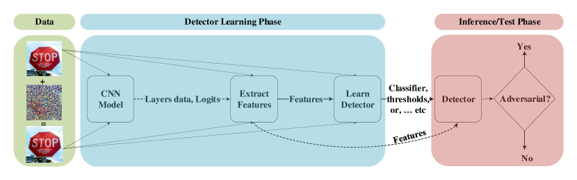
Figure 2: Abstract overview of learning a detector for a victim model. On one side, Data side, the adversary generates AE using adversarial attack algorithm with the help of knowledge that he got about the victim model. On the other side, in the Detector Learning Phase, the defender trains the detector using the information that he got from the victim model, training data, and/or attacked/adversarial data. In Inference/Test Phase, the adversary replaces the clean input with the adversarial one, then, the detector checks the input and recommend if it is clean or adversarial which should be rejected.

forked edges, for tree=draw,align=center,edge=-latex,fill=white,blur shadow, where level=1 for descendants=grow’=0, folder, l sep’+=2.5pt, , [AEs Detection Methods [Supervised [Network invariant [SafetyNet
lu2017safetynet ] [Histogram
pertigkiozoglou2018detecting ] [AEs
evolution
carrara2018adversarial ] [Dynamic
Adversary
Training
metzen2017detecting ] [RAID
eniser2020raid ] ] [Auxiliary model [Model
Uncertainty
feinman2017detecting ; smith2018understanding , draw=red!80, fill=red!10,] [Softmax
based
hendrycks2016baseline ; pertigkiozoglou2018detecting
aigrain2019detecting ; monteiro2019generalizable ] [Raw AEs
gong2017adversarial ; grosse2017statistical
hosseini2017blocking ; pertigkiozoglou2018detecting ] [Gradient
based
lust2020gran ] [NSS
kherchouche2020detection , draw=red!80, fill=red!10,] [E&R
zuo2020exploiting ] ] [Statistical [MMD
grosse2017statistical ] [PCA
li2017adversarial ] [KD
feinman2017detecting , draw=red!80, fill=red!10,] [LID
ma2018characterizing , draw=red!80, fill=red!10,] [$k$-NN
cohen2020detecting ] [Mahalanobis
lee2018simple ] ] ] [Unsupervised [Network invariant [NIC
ma2019nic , draw=red!80, fill=red!10,] ] [Object-based [UnMask
freitas2020unmask ] ] [Denoiser [PixelDefend
song2017pixeldefend ] [Magnet
meng2017magnet , draw=red!80, fill=red!10,] ] [Statistical [Softmax
based
hendrycks2016baseline ] [PCA
hendrycks2016early ] [GMM
zheng2018robust ] ] [Feature Squeezing [Bit-Depth
and
Smoothing
xu2017feature , draw=red!80, fill=red!10,] [Adaptive
Noise
Reduction
liang2017detecting ] ] [Auxiliary model [$k$-NN
classifier
carrara2017detecting ] [Reverse
Cross-Entropy
pang2018towards ] [Uncertainty
sheikholeslami2019minimum ] [DNR
sotgiu2020deep , draw=red!80, fill=red!10,] [SFAD
aldahdooh2021selective , draw=red!80, fill=red!10,] ] ] ]

Figure 3: Categories of Adversarial Examples Detection Methods. The highlighted red rectangles are the detection methods considered in the experimental study.

Table 3: Summary of state-of-the-art detection methods and the corresponding detection accuracy performance as reported in their original paper. M=MINIST, C=CIFAR-10, S=SVHN, I=ImageNet and TI=Tiny-ImageNet. Detection rate in average: $\bigstar\bigstar\bigstar\bigstar\bigstar$=90-100, $\bigstar\bigstar\bigstar\bigstar$=80-89, $\bigstar\bigstar\bigstar$=70-79, $\bigstar\bigstar$=50-69, and $\bigstar$=0-49

Category	Sub Category	Model	Tested against	Performance Notes
Supervised	Auxiliary model	Uncertainty feinman2017detecting	FGSM, BIM, CW, JSMA	M($\bigstar\bigstar\bigstar\bigstar$), C($\bigstar\bigstar$), S($\bigstar\bigstar$), Circumventable carlini2017adversarial
		Softmax pertigkiozoglou2018detecting	BIM, DF	M($\bigstar\bigstar\bigstar\bigstar\bigstar$)
		Softmax aigrain2019detecting	FGSM, BIM, DF	M($\bigstar\bigstar\bigstar\bigstar\bigstar$), C($\bigstar\bigstar\bigstar\bigstar\bigstar$)
		Softmax monteiro2019generalizable	FGSM, BIM, JSMA, DF	M($\bigstar\bigstar\bigstar\bigstar\bigstar$), C($\bigstar\bigstar\bigstar\bigstar\bigstar$)
		Raw AEs gong2017adversarial	FGSM, BIM	M($\bigstar\bigstar\bigstar\bigstar\bigstar$), C($\bigstar\bigstar\bigstar\bigstar\bigstar$), S($\bigstar\bigstar\bigstar\bigstar\bigstar$), Circumventable carlini2017adversarial
		Raw AEs grosse2017statistical	FGSM, JSMA,	M($\bigstar\bigstar\bigstar\bigstar\bigstar$), Circumventable and bad performance for CIFAR-10 carlini2017adversarial
		Raw AEs pertigkiozoglou2018detecting	BIM, DF	M($\bigstar\bigstar\bigstar\bigstar$)
		NSS kherchouche2020detection	FGSM, BIM, CW, DF	M($\bigstar\bigstar\bigstar\bigstar\bigstar$), C($\bigstar\bigstar\bigstar\bigstar\bigstar$), I($\bigstar\bigstar\bigstar\bigstar\bigstar$)
		Gradient lust2020gran	FGSM, BIM, JSMA, CW	M($\bigstar\bigstar\bigstar\bigstar\bigstar$), C($\bigstar\bigstar\bigstar\bigstar\bigstar$), S($\bigstar\bigstar\bigstar\bigstar\bigstar$)
		E&R zuo2020exploiting	CW, DF	C($\bigstar\bigstar\bigstar\bigstar\bigstar$), I($\bigstar\bigstar\bigstar\bigstar\bigstar$)
	Statistical	MMD grosse2017statistical	FGSM, JSMA	MNIST($\bigstar\bigstar\bigstar\bigstar\bigstar$), Circumventable carlini2017adversarial
		PCA li2017adversarial	L-BFGS,	I($\bigstar\bigstar\bigstar\bigstar$), Circumventable carlini2017adversarial and bad performance for M and C
		KD feinman2017detecting	FGSM, BIM, CW, JSMA	M($\bigstar\bigstar\bigstar\bigstar$), C($\bigstar\bigstar\bigstar\bigstar$), S($\bigstar\bigstar$), Circumventable carlini2017adversarial
		LID ma2018characterizing	FGSM, BIM, JSMA	M($\bigstar\bigstar\bigstar\bigstar\bigstar$), C($\bigstar\bigstar\bigstar\bigstar\bigstar$), S($\bigstar\bigstar\bigstar\bigstar\bigstar$), Circumventable athalye2018obfuscated
		Mahalanobis lee2018simple	FGSM	C($\bigstar\bigstar\bigstar\bigstar\bigstar$), S($\bigstar\bigstar\bigstar\bigstar\bigstar$)
		$k$-NN cohen2020detecting	FGSM, JSMA, DF, PGD, CW	C($\bigstar\bigstar\bigstar\bigstar\bigstar$), S($\bigstar\bigstar\bigstar\bigstar\bigstar$)
	Network invariant	Safetynet lu2017safetynet	FGSM, BIM, DF	C($\bigstar\bigstar\bigstar\bigstar$), I($\bigstar\bigstar\bigstar$)
		Histogram pertigkiozoglou2018detecting	BIM, DF	M($\bigstar\bigstar\bigstar\bigstar$)
		Dynamic Adversary Training metzen2017detecting	FGSM, BIM, DF	C($\bigstar\bigstar\bigstar\bigstar$), I($\bigstar\bigstar\bigstar$), Circumventable carlini2017adversarial
		AEs evolution carrara2018adversarial	L-BFGS, FGSM, BIM, PGD	I($\bigstar\bigstar\bigstar\bigstar$)
		RAID eniser2020raid	FGSM, BIM, PGD, DF, CW, JSMA	M($\bigstar\bigstar\bigstar\bigstar$), C($\bigstar\bigstar\bigstar\bigstar\bigstar$)
Unsupervised	Auxiliary model	$k$-NN carrara2017detecting	L-BFGS, FGSM,	I($\bigstar\bigstar\bigstar\bigstar$)
		Reverse Cross-Entropy pang2018towards	FGSM, BIM, CW, JSMA	M($\bigstar\bigstar\bigstar\bigstar\bigstar$), C($\bigstar\bigstar\bigstar\bigstar\bigstar$)
		Uncertainty sheikholeslami2019minimum	FGSM, BIM, CW	C($\bigstar\bigstar\bigstar\bigstar$)
		DNR sotgiu2020deep	optimized-PGD,	M($\bigstar\bigstar\bigstar$), C($\bigstar$)
		SFAD aldahdooh2021selective	FGSM, PGD, CW, DF	M($\bigstar\bigstar\bigstar\bigstar\bigstar$), C($\bigstar\bigstar\bigstar$)
	Statistical	PCA hendrycks2016early	FGSM, BIM	M($\bigstar\bigstar\bigstar\bigstar\bigstar$), Circumventable carlini2017adversarial and not effective for CIFAR-10
		GMM zheng2018robust	FGSM,	MNIST($\bigstar\bigstar\bigstar\bigstar\bigstar$)
	Denoiser	PixelDefend song2017pixeldefend	FGSM, BIM, DF, CW	C($\bigstar\bigstar\bigstar\bigstar$), Circumventable athalye2018obfuscated
		MagNet meng2017magnet	FGSM, BIM, DF, CW	M($\bigstar\bigstar\bigstar\bigstar\bigstar$), C($\bigstar\bigstar\bigstar\bigstar$), Circumventable carlini2017magnet
	Feature Squeezing	Bit-Depth and Smoothing xu2017feature	FGSM, BIM, DF, CW, JSMA	M($\bigstar\bigstar\bigstar\bigstar\bigstar$), C($\bigstar\bigstar$), I($\bigstar\bigstar\bigstar$)
		Adaptive Noise Reduction liang2017detecting	FGSM, CW, DF	M($\bigstar\bigstar\bigstar\bigstar\bigstar$), I($\bigstar\bigstar\bigstar\bigstar\bigstar$)
	Network invariant	NIC ma2019nic	FGSM, BIM, DF, CW, JSMA	M($\bigstar\bigstar\bigstar\bigstar\bigstar$), C($\bigstar\bigstar\bigstar\bigstar\bigstar$), I($\bigstar\bigstar\bigstar\bigstar\bigstar$)
	Object-Based	UnMask freitas2020unmask	BIM, PGD	I($\bigstar\bigstar\bigstar\bigstar$)

4.1 Supervised detection

In supervised detection, the defender considers AEs generated by one or more adversarial attack algorithms in designing and training the detector   $\mathcal{D}$. It is believed that AEs have distinguishable features that make them different from clean inputs ilyas2019adversarial , hence, defenders take this advantage to build a robust detector $\mathcal{D}$. To accomplish this, many approaches have been presented in the literature.

4.1.1 Auxiliary model approach

In this approach, models exploit features that can be extracted by monitoring the clean and adversarial samples behaviors. Then, either classifiers or thresholds are built and calculated.

Model uncertainty. Defenders are using DL models uncertainty of clean and adversarial inputs. The uncertainty is usually measured by adding randomness to the model using Dropout srivastava2014dropout technique. The idea is that with many dropouts, clean input class prediction remains correct, while it is not with AEs. Uncertainty values are used as features to build a binary classifier as a detector $\mathcal{D}$. Feinman et al. feinman2017detecting proposed bayesian uncertainty (BU) metric, which uses Monte Carlo dropout to estimate the uncertainty, to detect those AEs that are near the classes manifold, while Smith et al. smith2018understanding used mutual information method for such task.

Softmax/logits-based. Hendrycks et al. hendrycks2016baseline showed that softmax prediction probabilities can be used to detect abnormality, they append a decoder to reconstruct clean input from the softmax and trained it jointly with the baseline classifier. Then, they train a classifier, a detector $\mathcal{D}$, using the reconstructed input, logits and confidence scores for clean and AEs inputs. In one of the methods that were proposed in pertigkiozoglou2018detecting , Pertigkiozoglou et al.used model vector features, i.e., confidence outputs, to calculate regularized vector features. The baseline classifier is retrained by adding this regularized vector features to the last layer of the classifier. The detector $\mathcal{D}$ considers an input as AE if there is no match between baseline classifier and the retrained classifier. Aigrain et al. aigrain2019detecting built a simple NN detector $\mathcal{D}$ which takes the baseline model logits of clean and AEs as inputs to build a binary classifier. Finally, following the hypothesis that different models make different mistakes when presented with the same attack inputs, Monteiro et al. monteiro2019generalizable proposed a bi-model mismatch detection. The detector $\mathcal{D}$  is a binary radial basis function (RBF)- support vector machine (SVM) classifier. Its inputs are the output of two baseline classifiers of clean and AEs.

Raw AEs-based classifier. Gong et al. gong2017adversarial trained a binary classifier, detector $\mathcal{D}$, that is completely separated from the baseline classifier and takes as input the clean and adversarial images. In grosse2017statistical ; hosseini2017blocking , the authors retrained the baseline classifier with a new added class, i.e., adversarial class. Hosseini et al.employed adversarial training and the used training labels are performed using label smoothing szegedy2015rethinking . In one of the methods that were proposed in pertigkiozoglou2018detecting , the authors took advantage of the DL model input’s parts that are ignored by the model to detect the AEs. They iteratively perturbed the input, clean or adversarial, and if the probability of the predicted input class is less than the threshold, then the input is declared as adversarial.

nss. natural scene statistics (NSS) has been used in many areas of image processing, especially in image quality estimation, since it has been proved that statistics of natural images are different from those of manipulated images. Kherchouche et al. kherchouche2020detection followed this assumption and built a binary classifier that takes as input features parameters of the Generalized Gaussian Distribution (GGD) and Asymmetric Generalized Distribution (AGGD) computed from the mean subtracted contrast normalized (MSCN) coefficients mittal2012no of clean images and PGD-based AEs.

Gradient based. Lust et al. lust2020gran proposed a detector $\mathcal{D}$ named GraN. At each layer, they calculated the gradient norm of a smoothed input, clean and adversarial, with respect to the predicted class of the baseline classifier. Then, they train a binary classifier $\mathcal{D}$ to detect AEs in inference time.

Erase&restore (E&R) zuo2020exploiting . In this model, Zuo et al.proposed a binary classifier, a detector $\mathcal{D}$, to train clean and $L_{2}$-norm adversarial samples after processing. Firstly, the input samples are processed by erasing some pixels and restoring them in an inpainting process. Secondly, the confidence probability is calculated using the baseline classifier. Finally, the processed confidence probability is then passed to the binary classifier. The detector $\mathcal{D}$ announces an input as adversarial if the binary classifier says so.

4.1.2 Statistical approach

In this approach, different statistical properties of clean and AEs inputs are calculated and then used to build the detector. These properties are more related to in- or out- of training data distribution/manifolds. The following statistical approaches are used in the literature:

mmd. Grosse et al. grosse2017statistical employed a statistical test, called maximum mean discrepancy (MMD) gretton2012kernel , to distinguish adversarial examples from the model’s training data. It is model-agnostic and kernel-based two-sample test. To answer the hypothesis test assumption, the detector $\mathcal{D}$ firstly computes the MMD between clean and AEs samples, $a=MMD(x,x^{\prime})$. Then, shuffle the elements of $x$ and $x^{\prime}$ into two new sets $y_{1}$ and $y_{2}$, and compute $b=MMD(y_{1},y_{2})$. Finally, conclude that $x$ and $x^{\prime}$ are drawn from different distributions and reject the hypothesis if $a<b$.

pca. The work in li2017adversarial built cascade classifiers. Each SVM classifier corresponds to one layer. It is trained using clean and AEs samples. The input of the SVM is the principal component analysis (PCA) of each layer output. The detector $\mathcal{D}$ announces an input as clean if all classifiers say so.

kd. It was shown that AEs subspaces usually have lower density than clean samples especially if the input sample is far from a class manifold. Feinman et al. feinman2017detecting proposed kernel density (KD) estimation for each class in the training data and then trained a binary classifier, detector $\mathcal{D}$, using densities and uncertainties features of clean, noisy, and AEs.

lid. As an alternative measure to KD, Ma et al.in ma2018characterizing used local intrinsic dimensionality (LID) to calculate the distance distribution of the input sample to its neighbors to assess the space-filling capability of the region surrounding that input sample.

Mahalanobis-based. As an alternative measure to KD and LID, Lee et al. lee2018simple proposed Mahalanobis distance-based score to detect out-of-distribution and adversarial input samples. This confidence score is based on an induced generative classifier under gaussian discriminant analysis (GDA) that actually replaces the softmax classifier.

knn. The work in cohen2020detecting firstly measured the impact/influence of every training sample on the validation set data and then found the most supportive training samples for any given validation example. Then, at each layer, using the DL layers representative output, a k-nearest neighbor ($k$-NN) model is fitted to rank these supporting training samples. These features are extracted from clean and AEs to train a detector $\mathcal{D}$. Recently, Mao et al. mao2020learning proposed Neighbor Context Encoder (NCE) detector. It used transformer vaswani2017attention to train a classifier with $k$ nearest neighbors to represent the surrounded subspace of the detected sample.

4.1.3 Network invariant approach

It is believed that the clean and the adversarial samples yield different feature maps and different activation values for the network layers. Analysing this network invariant violation is the core components for many detection methods.

Safetynet lu2017safetynet . SafetyNet states the hypothesis “Adversarial attacks work by producing different patterns of activation in late stage ReLUs to those produced by natural examples”. Hence, SafetyNet quantizes the last ReLU activation layer of the model and builds a binary SVM RBF classifier.

Dynamic adversary training metzen2017detecting . Metzen et al.presented dynamic adversary training to harden the detector in which the classifier was trained with AEs. The detector $\mathcal{D}$ is augmented to the pre-trained classifier at a specific layer output. It takes layer’s representative output for clean samples and for on fly generated AEs as input to build a binary classifier.

Histogram-based pertigkiozoglou2018detecting . Pertigkiozoglou et al.observed that for AEs there is an increase in the values of some peaks of clean output while there is a decrease in the values on the rest of the points of the output. Hence, they built a binary SVM classifier which takes as inputs the histogram of the first convolutional layer output of the baseline classifier for clean and AEs.

AEs evolution carrara2018adversarial . Carrara et al.hypothesized that intermediate representations of AEs follow a different evolution with respect to clean inputs. The detector $\mathcal{D}$  encodes the relative positions of internal activations of points that represent the dense parts of the feature space. The detector is a binary classifier built on top of the pre-trained network and takes as inputs the encoded relative positions of internal activations of points that represent the dense parts of the feature space for AEs and clean inputs.

RAID eniser2020raid . Eniser et al.built a binary classifier that takes as inputs the differences in neuron activation values between clean and AEs inputs. In order to make the adaptive attacks much harder, the authors also provided an extension to RAID called Pooled-RAID. This latter aims at training a pool of detectors, each trained with a randomly selected number of neurons. In the test time, the Pooled-RAID selects randomly one detection classifier from the pool to test if the input is adversarial or not.

4.2 Unsupervised detection

The main limitation of supervised detection methods is that they require prior knowledge about the attacks and hence they might not be robust against new/unknown attacks. In unsupervised detection, the defender considers only the clean training data in designing and training the detector $\mathcal{D}$. It is also known as inconsistency prediction models since it depends on the fact that AEs might not fool every NN model.
Basically, unsupervised detectors aim at reducing the limited input feature space available to adversaries and to accomplish this goal, many approaches have been presented in the literature.

4.2.1 Auxiliary model approach

Unlike auxiliary models of supervised detection, unsupervised models exploit features that can be concluded by monitoring only the clean samples behaviors. Then, either classifiers or thresholds are built and calculated.

knn classifier carrara2017detecting . Carrara et al.used the output of one of the intermediate DL model layers to build a $k$-NN classifier. The output of this classifier is not used for the detection, but it is used to score the predicted class of baseline classifier. The detector $\mathcal{D}$ announces the input is adversarial if this score is less than a specified threshold. They also provided a process to use the PCA of the output of one of the intermediate DL model layers to reduce the feature dimension.

Reverse cross-entropy pang2018towards . Pang et al.proposed a training procedure and a threshold-based detector. Firstly, the baseline classifier is retrained with a reverse cross-entropy loss function in order to better learn latent representations that will distinguish clean inputs and AEs. Then, for each class, a kernel density is estimated and, then, the threshold is calculated. Finally, the detector $\mathcal{D}$announces an input as adversarial if its density score is less than the calculated threshold. The authors in pang2018towards also introduced an alternative estimation of Kernel density called Non-maximal entropy but they found that detection using kernel density estimation gives better results than non-ME Non-maximal entropy in most of the cases.

Uncertainty-based. Following BU assumption that AEs distances from in-distribution data make the DL model uncertainty differs from clean data, Sheikholeslami et al. sheikholeslami2019minimum proposed to introduce randomness for randomly sampled hidden units of each layer of DL model. Then, the uncertainty is estimated for in-distribution training data and a mutual information based threshold is identified. They provided a layer-wise minimum variance solver to estimate the uncertainty. At inference time, the input image overall uncertainty is estimated using the hidden layers outputs. Detector $\mathcal{D}$ announces the input sample as adversarial if its mutual information is larger than the threshold.

dnr sotgiu2020deep . Sotgiu et al.proposed to use the $N$-last representative layers outputs of the baseline classifiers to build $N$-SVM classifiers with RBF kernel. The output of these classifiers, i.e., the confidence probabilities, are combined to build the last classification task classifier which is an SVM-RBF classifier. The detector $\mathcal{D}$ announces an adversarial input as adversarial if the maximum confidence probability is less than a predefined threshold.

Selective detection aldahdooh2021selective . Aldahdooh et al.proposed selective and feature based adversarial detection (SFAD) technique. They use the recent uncertainty method called SelectiveNet selective2019 and integrated three detection modules. The first is the selective detection module, which is a threshold-based detection derived from uncertainty of clean training data using SelectiveNet. The second is confidence detection module, which is threshold-based detection derived from softmax probabilities of clean training data from SFAD’s classifiers. SFAD’s classifiers analyse the representative data of last $N$-layers as a key point to present robust features of input data using autoencoding, up/down sampling, bottleneck, and noise blocks. The last module is ensemble prediction, which is a mismatch-based prediction between the detector and the baseline DL classifiers.

4.2.2 Statistical approach

In this approach, different statistical properties of only clean inputs are calculated and then used to build the detector. These properties are more related to in- or out- of training data distribution/manifolds. The following statistical approaches are used in the literature:

Softmax distribution hendrycks2016baseline . Hendrycks et al.found that maximum/predicted class probability of in-distribution samples are higher than of out-of-distribution. This information is used and Kullback-Leibler divergence kullback1951information is computed between in-distribution and clean input samples to determine the threshold.

PCA hendrycks2016early . Hendrycks et al.observed that the later PCA components variance of AEs is larger than those of clean inputs, hence, they proposed a detector $\mathcal{D}$ to declare the input as adversarial if the later PCA components variance is above the threshold.

Gaussian mixture model (GMM) zheng2018robust . Zheng et al.proposed a detection method called I-defender, referred here as “intrinsic”. It explores the distributions of DL model hidden states of the clean training data. I-defender uses GMM to approximate the intrinsic hidden state distribution of each class. I-defender chooses to only model the state of the fully connected hidden layers and then a threshold for each class is calculated. The detector $\mathcal{D}$ announces the input sample as adversarial if its hidden state distribution probability is less than the predicted class’s threshold. On the other hand, the work in miller2019not works under the assumption that the adversarial input 1) has atypically low likelihood compared to the density model of predicted class and is called “too atypical”, and 2) has high likelihood for a class other than the class of clean input and is called “too typical”. Hence, for each case, a two-class posterior is evaluated, i.e., one with respect to the density estimation and one with respect to the DL model. The final score for “too atypical” and “too typical” are calculated using the Kullback-Leibler divergence. The detector $\mathcal{D}$  declares an input as adversarial if the score is larger than the predefined threshold.

4.2.3 Denoiser approach

To prevent the adversary from estimating the location of AEs accurately, one can make the input gradient very small or irregularly large. This phenomenon is known as exploding/vanishing gradients. One method to do that is to denoise or reconstruct AEs to maximize the ability to project the AEs to the training data manifold. The main limitation of using denoiser is that it is not guaranteed to remove all the noise to produce highly denoised inputs, and it might introduce extra distortion. Besides, it is not effective in denoising the $L_{0}$ attacks, since $L_{0}$ attacks target a few pixels and these pixels might not be denoised by the denoiser.

PixelDefend song2017pixeldefend . Generative models such as PixelCNN van2016conditional explode the gradient by applying cumulative product of partial derivatives from each layer. PixelDefend detection song2017pixeldefend utilised PixelCNN to build its detector. Firstly, PixelDefend reconstructs/purifies the clean training data using PixelCNN and then computes the prediction probabilities using baseline classifier. It is found that reconstructed images have higher probabilities under in-distribution of training data. Then, the probability density of the training samples are computed. The detector $\mathcal{D}$ works by, firstly, computing the probability density of tested input. Secondly, this density is ranked with training data densities. Finally, the rank can be used as a test statistic, and $p$-value is calculated to determine if the input sample belongs to the in-distribution of training data or it is adversarial.

Magnet meng2017magnet . Magnet trains denoisers in clean training data to reconstruct the input samples. Magnet proposed two ways to detect AEs. The first one assumes that the reconstruction error will be small for clean images and large in AEs and hence, it calculates the reconstruction error as a score. The second way measures the distances between the predictions of input samples and their denoised/filtered versions. The detector $\mathcal{D}$ announces the input sample as adversarial if the score exceeds a predefined threshold.

4.2.4 Feature Squeezing approach

This approach aims at squeezing out unnecessarily features of input samples to destroy perturbations. This process will limit the features space available for the adversary but if the squeezer is not built efficiently, it may enlarge the perturbation.

Bit-depth and smoothing xu2017feature . Xu et al.squeezes the input samples by projecting/transforming it to produce new samples. They used color bit-depth reduction, local smoothing using median filter and non-local smoothing filter using non-local mean denoiser. The detector $\mathcal{D}$ considers the input as adversarial if the distance between predicted original input and the squeezed version exceeds the identified threshold.

Adaptive noise reduction liang2017detecting . Liang et al.on the other hand, squeezes the input samples using scalar quantization and smoothing spatial filter. They used the image entropy as a metric to implement the adaptive noise reduction. The detector $\mathcal{D}$  considers the input as adversarial if the class of original input is different from the squeezed version.

4.2.5 Network invariant approach

Unlike the network invariant approach of supervised detection, here, the detector aims at observing behaviors of clean training data only in the intermediate DL model layers. The recent work of Ma et al.ma2019nic showed that if the two attack channels, the provenance channel and the activation value distribution channel, are monitored, then the AEs can be detected. Ma et al.ma2019nic proposed a neural-network invariant checking (NIC) method that builds a set of models for individual layers to describe the provenance and the activation value distribution channels. The provenance channel describes the instability of activated neurons set in the next layer when small changes are present in the input sample, while the activation value distribution channel describes the changes with the activation values of a layer. To train the invariant models, the authors used One-Class Classification (OCC) problem as a way to model in-distribution training data. The detector $\mathcal{D}$ is a joint OCC classifier that joins all invariant models’ outputs. It announces the input sample as adversarial if the detector classifier declares the input is out-of-distribution.

4.2.6 Object-based approach

In this approach, the aim is to extract object-based features from the input sample and compare them with training data of the same prediction label. UnMask is a method proposed by Freitas et al. freitas2020unmask that works as follows: firstly, assume the adversary altered a bicycle image to be predicted as a bird. UnMask first extracts object-based low-level features from the attacked image “the bicycle” and compares them with object-based low-level features of “the bird”. Then, if there is a small overlap, the detector $\mathcal{D}$ will announce the input as adversarial. Also, Unmask continues “as a defense” to find which class in the training data classes has the highest overlap with the predicted one to announce the correct class.

5 Experiment settings

5.1 Datasets

In this work, we evaluate the detection methods on the following four datasets:

MNIST lecun1998gradient . It is a handwriting digit recognition dataset for digits from 0 to 9. It contains 70000 gray images/samples, 60000 for training and 10000 for testing.

SVHN netzer2011reading . It is a real street view house numbers recognition dataset. The numbers are cropped in digits of ten classes. It contains 99289 RGB images/samples, 73257 digits for training and 26032 digits for testing.

CIFAR-10 krizhevsky2009learning . It is a collection of images that is usually used in computer vision tasks. It is $32\times 32$ RGB images of ten classes: airplanes, cars, birds, cats, deer, dogs, frogs, horses, ships, and trucks. It contains 60000 images, 50000 for training and 10000 for testing.

Tiny ImageNet yao2015tiny . It is a tiny version of ImageNet imagenet_cvpr09 dataset. It contains $64\times 64$ RGB images and includes 200 classes. It is composed of 110,000 images, 100000 for training and 10000 for testing.

5.2 Baseline “Victim” classifiers

In order to evaluate the detection methods, we built and trained four baseline victim models, one for each dataset.

MNIST. We built and trained a 6-layer CNN classifier for this dataset. It achieves state of the art results of 98.73% accuracy. We follow the architecture that is described in sotgiu2020deep and shown in Table 4.

SVHN. We built and trained a 6-layer CNN classifier, similar to MNIST, for the SVHN dataset. It achieves state of the art results of 94.99% accuracy. We use similar architecture of the MNIST and we only changed the number of neurons of the dense layers as shown in Table 5.

CIFAR10. Since the CIFAR10 dataset is not a complex task, we did not use complex CNN architecture to avoid the phenomena of the CNN not using saliency regions of clean images in predicting the correct classmadry2017towards . We follow the architecture that is described in sotgiu2020deep and shown in Table 6. An 8-layer CNN classifier was built and trained for CIFAR10 dataset. It achieves accuracy of 89.11%.

Tiny-ImageNet. We use a classifier relying on DenseNet201 huang2017densely , one of the state-of-the-art classifiers for image classification. We started with the DenseNet201 weights of ImageNet and then the model was fine-tuned for a 200-class classification task. It achieves 65% classification accuracy.

Table 4: MNIST baseline classifier architecture.

#	Layer	Description
1	Conv2D + ReLU	32 filters ($3\times 3$)
2	Conv2D + ReLU + Max Pooling($2\times 2$)	32 filters ($3\times 3$)
3	Conv2D + ReLU	64 filters ($3\times 3$)
4	Conv2D + ReLU + Max Pooling($2\times 2$)	64 filters ($3\times 3$)
5	Dense + ReLU + Dropout ($p=0.3$)	256 units
6	Dense + ReLU	256 units
7	Dense + Softmax	10 classes

Table 5: SVHN baseline classifier architecture.

#	Layer	Description
1	Conv2D + ReLU	32 filters ($3\times 3$)
2	Conv2D + ReLU + Max Pooling($2\times 2$)	32 filters ($3\times 3$)
3	Conv2D + ReLU	64 filters ($3\times 3$)
4	Conv2D + ReLU + Max Pooling($2\times 2$)	64 filters ($3\times 3$)
5	Dense + ReLU + Dropout ($p=0.3$)	512 units
6	Dense + ReLU	128 units
7	Dense + Softmax	10 classes

Table 6: CIFAR10 baseline classifier architecture.

#	Layer	Description
1	Conv2D + BatchNorm + ReLU	64 filters ($3\times 3$)
2	Conv2D + BatchNorm + ReLU + Max Pooling($2\times 2$) + Dropout ($p=0.1$)	64 filters ($3\times 3$)
4	Conv2D + BatchNorm + ReLU	128 filters ($3\times 3$)
5	Conv2D + BatchNorm + ReLU + Max Pooling($2\times 2$) + Dropout ($p=0.2$)	128 filters ($3\times 3$)
6	Conv2D + BatchNorm + ReLU	256 filters ($3\times 3$)
7	Conv2D + BatchNorm + ReLU + Max Pooling($2\times 2$) + Dropout ($p=0.3$)	256 filters ($3\times 3$)
8	Conv2D + BatchNorm + ReLU + Max Pooling($2\times 2$) + Dropout ($p=0.4$)	512 filters ($3\times 3$)
9	Dense	512 units
10	Dense + Softmax	10 classes

Table 7: Baseline classifiers’ accuracies on normal clean testing data and attacked($\epsilon$) data.

	Attack($\epsilon$)	Datasets
		MNIST	CIFAR	SVHN	Tiny
ImageNet
Clean
Data	-	98.73	89.11	94.98	64.48
White box	FGSM(8)	-	14.45	15.06	12.14
	FGSM(16)	-	13.66	5.91	8.11
	FGSM(32)	76.97	11.25	-	-
	FGSM(64)	13.76	-	-	-
	FGSM(80)	8.64	-	-	-
	BIM(8)	-	1.9	1.25	0.3
	BIM(16)	-	0.61	0	0
	BIM(32)	21.84	-	-	-
	BIM(64)	0	-	-	-
	BIM(80)	0	-	-	-
	PGD-$L_{1}$(5)	-	43.45	-	-
	PGD-$L_{1}$(10)	65.95	10.56	-	-
	PGD-$L_{1}$(15)	25.74	5.27	17.59	44.7
	PGD-$L_{1}$(20)	4.95	-	7.97	31.34
	PGD-$L_{1}$(25)	-	-	3.73	21.97
	PGD-$L_{2}$(0.25)	-	13.97	-	-
	PGD-$L_{2}$(0.3125)	-	8.19	35.5	-
	PGD-$L_{2}$(0.5)	-	5.52	13.26	8.46
	PGD-$L_{2}$(1)	70.54	-	0.8	1.34
	PGD-$L_{2}$(1.5)	18.89	-	-	-
	PGD-$L_{2}$(2)	0.79	-	-	-
	PGD-$L_{\infty}$(8)	-	0.78	0.8	0.02
	PGD-$L_{\infty}$(16)	-	0.28	0	0
	PGD-$L_{\infty}$(32)	19.05	-	-	-
	PGD-$L_{\infty}$(64)	0	-	-	-
	CW-$L_{\infty}$	38.98	20.95	23.73	16.64
	CW-HCA(8)	-	46.51	47.06	39.47
	CW-HCA(16)	-	18.96	29.06	17.51
	CW-HCA(80)	43.36	-	-	-
	CW-HCA(128)	8.64	-	-	-
	DF	4.96	4.8	6.12	0.52
	JSMA	0	0	0	0.3
Black box	SA	4.66	0	0.7	0.22
	HopSkipJump	0	0	0	0
	ST	22.04	52.57	17.0	52.28
	PA	7.7	7.9	9.8	0.5

5.3 Threat Model and Attacks

Here, we define the environment that the adversary faces to generate the AEs. It is assumed that the adversary has zero-knowledge about the detection methods. Then, he might generate, using available information on the victim model, white box attacks, black box attacks and gray box attacks. We use the ART art2018 library to generate the attacks under all tested datasets.

White box attacks. Different $L_{p}$-norm attacks are used to test the detection methods. JSMA is used to generate $L_{0}$ attacks (only 1500 samples for Tiny-ImageNetdataset). For $L_{1}$ attacks, $L_{1}$ PGD attack is used. For $L_{2}$ attacks, PGD, CW/HCA and DF $L_{2}$ attacks are used. For $L_{\infty}$ attacks, FGSM, BIM, PGD and CW $L_{\infty}$ attacks are considered. For FGSM, BIM and PGD attacks, the $\epsilon=\{8,$ $16,$ $32,$ $64,$ $80,$ $128\}$ is set to each dataset as shown in Table 7. For CW attack, 200 iterations and zero confidence setting are used.

Black box attacks. PA su2019one , SA andriushchenko2020square , HopSkipJump  chen2020hopskipjumpattack and ST engstrom2019exploring black box attacks are generated in the testing process. The translation and rotation values of ST attack are set to 10 and 60 for MNIST and SVHN, and to 8 and 30 for CIFAR and Tiny-ImageNet, respectively. For SA attack, the epsilon ($\epsilon$) is set to $32-80$ out of 255. For HopSkipJump attack, untargeted and unmasked attack is considered, besides, 40 and 100 are set for iterations steps and maximum evaluations, respectively. For PA attacks, only 1000 AEs for each dataset are generated.

Gray box attacks. In order to evaluate the detection methods against gray box attacks, we built surrogate models of the baseline classifiers. For MNIST, SVHN and CIFAR10, surrogate classifiers are similar to victim classifiers with only one change that is a Dropout layer is added before the last Dense layer. For MNIST, the classification accuracy is 99.32%, for SVHN the classification accuracy is 95.48%, and for CIFAR10 the classification accuracy is 93.35%. For Tiny-ImageNet, ResNet50V2 he2016identity classifier is fine-tuned and it achieves accuracy of 51.7%. Then, the white box attacks are generated under the surrogate classifiers.

Untargeted Attack. All the tested attacks in this work are untargeted attacks. It was shown that untargeted attacks 1) have less perturbations than targeted attacks 2) have better success rates, and 3) possess stronger transferability capability carlini2017towards ; liu2016delving .

Table 7 shows the baseline classifiers’ accuracy to the clean training data and the tested attacked data.

Robust attacks. As shown in carlini2017adversarial ; athalye2018obfuscated , detectors and defenses can be bypassed using different strategies such as; strong attacks, unknown attacks, or circumventing the detectors, especially for differential-basedclassifiers/detectors. In this work, we considered the method that is described in athalye2018obfuscated to break LID detector. The goal is to generate high confidence attacks carlini2017adversarial that minimize the $L_{\infty}$-norm under the zero-knowledge of the deployed defense.

5.4 Detection Methods

In our experiments, we retest all the following detection methods under the same environment. We choose to assess the performance of 8 different detection methods from different categories that are popular in the research communities and their source code are publicly available. We build a testing environment that combines all the tested methods and is publicly available. In this subsection, a technical description for each detector is provided with their configurations and hyper-parameters.

5.4.1 KD+BU feinman2017detecting :

The detector: For given clean and adversarial examples, noisy samples are crafted to be treated as clear samples. Then, Bayesian uncertainty scores is computed using Monte Carlo Dropout estimation for clean, noisy, and adversarial samples. Kernel density is estimated for each class using Gaussian estimation with specific bandwidth and then, kernel density scores are computed for clean, noisy and adversarial samples. Finally, a logistic regression classifier is trained using uncertainty and density scores.

Settings: The following settings are considered:

• To generate noisy samples: Gaussian noise is added to each pixel with a scale that is set to be equal to the $L_{p}$–norm of the adversarial perturbation. For $L_{0}$ attacks, an equal number of pixels that were altered in the adversarial example are flipped randomly.

• For kernel density estimation: the bandwidth parameter is tuned and set to be 1.26, 0.26, 1 and 0.26 for MNIST, CIFAR, SVHN and Tiny-ImageNet datasets, respectively.

• 70% of testing data is used to train the detector and 30% of testing data is used to test the detector.

• The adversarial examples for both training and testing were generated by applying one of the attacks at a time.

5.4.2 LID ma2018characterizing :

The detector: For given clean and adversarial examples, noisy samples are crafted to be treated as clear samples. Then, for each sample the LID score is calculated for $k$-neighbor samples. Finally, a logistic regression classifier is trained using LID scores.

Settings: The following settings are considered:

• To generate noisy samples: same procedures of KD+BU are applied.

• The $k$-neighbor is set to 20 for MNIST and SVHN, and 30 for CIFAR and Tiny-ImageNet.

• 70% of testing data is used to train the detector and 30% of testing data is used to test the detector.

• The adversarial examples for both training and testing were generated by applying one of the attacks at a time.

5.4.3 NSS kherchouche2020detection :

The detector: For given clean samples, AEs are generated using PGD attack with different perturbation radius $\epsilon$. For the clean and the adversarial examples, 18 features from the asymmetric generalized distribution (AGGD) are then computed using mean subtracted contrast normalized (MSCN) coefficients. Finally, a binary SVM classifier is trained using these 18 features.

Settings: The following settings are considered:

• To generate the AEs using PGD attack: we divide the clean testing data into six groups and the PGD-based AEs for each group are generated using $\epsilon=\{0.03125,$ $0.0625,$ $0.125,$ $0.25,$ $0.3125,$ $0.5\}$, respectively.

• For the SVM classifier, the regularization parameter $C$ and the kernel coefficient $g$/gamma of the classifier are tuned using grid search.

5.4.4 FS xu2017feature :

The detector: Once squeezers are defined, squeezed clean samples are generated. The maximum $L_{1}$ or $L_{2}$ distance is computed between the prediction probabilities of clean and squeezed samples. Finally, the threshold value with a specific false positive rate is computed.

Settings: The following settings are considered:

• Squeezers: 1) Color bit depth reduction. 2) Median smoothing filter 3) Non-local mean denoiser.

  • Color bit depth reduction: 1-bit for MNIST and 5-bit for SVHN, CIFAR, and Tiny-ImageNet

  • Median smoothing filter: $2\times 2$ size filter for all datasets.

  • Non-local mean denoiser: search window = 13, block size = 3, and filter strength for luminance component = 2 for all datasets except MNIST. For MNIST dataset, the non-local mean denoiser is not used.

• Detector training: 50% of test data is used for detector training.

• False positive rate: 5%

5.4.5 MagNet meng2017magnet :

The detector: Here, we demonstrate the detection process only of MagNet without the defense process. For given clean training samples, one or more autoencoders are trained. For a given clean validation data, calculate the $L_{1}$ reconstruction error using the autoencoders. Then, for each autoencoder, calculate the threshold value from the calculated reconstruction errors with a specific false positive rate.

Settings: The following settings are considered:

• Detector Autoencoders: two detectors are used

  • The first autoencoder structure: [Conv2D($3\times 3$), average pooling, Conv2D($3\times 3$), Conv2D($3\times 3$), up sampling, Conv2D($3\times 3$)].

  • The second autoencoder structure: [Conv2D($3\times 3$), Conv2D($3\times 3$)].

• 5000 samples from clean training samples are dedicated for validation process.

• False positive rate: 1% for MNIST and 5% for other datasets.

• We report only the results of the detector without taking into consideration the defense part, i.e., classification accuracy after applying the reformer. Please note that the original paper report the overall performance of the detection and the defense

5.4.6 deep neural rejection (DNR) sotgiu2020deep :

The detector: For given clean training samples, train three image classification classifiers using RBF-SVM. Each classifier receives, as input, the feature map(s) of a specific baseline classifier layer(s). Train a fourth image classification classifier using RBF-SVM. The classifier takes, as input, the prediction probabilities of the three classifiers trained in the first step. Given clean testing samples, get the maximum prediction probabilities and then calculate the threshold value from prediction probabilities for a given false positive rate.

Settings: The following settings are considered:

• Input of	MNIST, SVHN	CIFAR	Tiny-ImageNet
  $1^{st}$ classifier	Layer 4	Layer 7	Layer pool4_bn
  $2^{nd}$ classifier	Layer 5	Layer 8	Layer conv5_block17_0_bn
  $3^{rd}$ classifier	Layer 6	Layer 9	Layer bn

• See Tables 4-6 for Layer numbers.

• For the SVM classifiers, the regularization parameter $C$ is set to 1 and the kernel coefficient $\gamma$ is set to scale, where $scale=\frac{1}{F.V}$, $F$ is the number of features, and $V$ is the variance of the inputs

• False positive rate: 10%

5.4.7 SFAD aldahdooh2021selective :

The detector: For given clean training samples, three image classification classifiers are trained using SelectiveNet as described in Section 4.2.1. Each classifier receives, as input, the feature map(s) of a specific baseline classifier layer(s). The feature maps are processed during the training using autoencoding, up/down sampling, bottleneck, and noise blocks. A fourth image classification classifier is trained using SelectiveNet. The classifier takes, as input, the prediction probabilities of the three classifiers trained in the first step. Given clean testing samples, get the maximum prediction probabilities, and the selective probabilities. Finally, threshold values are computed from probabilities of the three classifiers for a given false positive rate.

Settings: The following settings are considered:

• Classifiers’ inputs are the same as DNR detector.

• The {coverage, coverage threshold} for SelectiveNet classifiers are set to:

• SelectiveNet	MNIST,	CIFAR, SVHN	Tiny-ImageNet
  $1^{st}$, $2^{nd}$, and $3^{rd}$ classifiers	{1, 0.995}	{0.9, 0.9}	{0.8, 0.5}
  $4^{th}$ classifier	{1, 0.7}	{0.9, 0.7}	{0.8, 0.5}

• False positive rate: 10%

5.4.8 NIC ma2019nic :

The detector: For given clean training samples and for each layer in the baseline model, get the feature map/‘provenance invariant (PI)’. Train PI classifier, OneClassSVM classifier, for each layer using layer feature’s map. Get the prediction probabilities/’activation values invariant (VI)’ for the current layer and the next layer. Train VI classifier, OneClassSVM classifier, for each layer using the prediction probabilities. Finally, train NIC classifier, OneClassSVM classifier, using the decision values of all PIs and VIs classifiers.

Settings: The following settings are considered:

• For provenance invariant channel classifiers, we use the first 5000 PCA components as features if the layer has more than 5000 features and we use $\nu=0.01$ and $\gamma=1$ for the OneClassSVM classifiers of all layers.

• For the activation value invariant channel and for the final NIC classifiers, we use $\nu=0.1$ and $\gamma=scale$, where $scale=\frac{1}{F.V}$, $F$ is the number of features, and $V$ is the variance of the inputs, for the OneClassSVM classifiers for all layers.

5.5 Performance measures

As discussed in Section 4, there are many criteria to assess the performance of detectors. In our experiment, we use detection rate (DR) and false positive rate (FPR) as two main performance evaluations. Other performance evaluation measures, like complexity (CM), overhead (OV) and inference time latency (INF) will be discussed as well.

6 Results and discussions

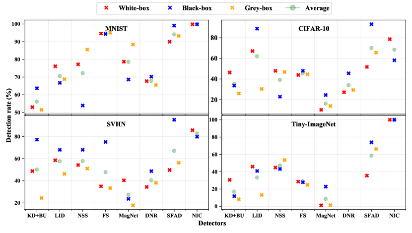
Figure 4: The average detection rate of eight detectors assessed against white-, black- and gray-box attacks scenarios. The green points represent the average over all scenarios.

In this section, we evaluate the performance of the detection methods on different datasets against different types of successful attack scenarios, white, black and gray box attacks. Tables 8, 9, 10 and 11 show detection rate and false positive rate (FPR) of the tested detectors on MNIST, CIFAR, SVHN and Tiny-ImagNet datasets, respectively, against white box attacks. Tables 12, 13, 14 and 15 show results for black box attacks, while Tables 16, 17, 18 and 19 show results for gray box attacks. The summary of all the experiments is shown in Figure 4.

In the following subsections, for each detection method, the performance results will be discussed for each attack scenario.

6.1 KD+BU feinman2017detecting

White box attacks. In general, the detector jointly combines density and uncertainty estimations. Basically, it is a two-feature binary classifier. AEs with low density probability and high uncertainty will be easily detected and that is obvious for BIM and PGD-$L_{\infty}$ attacks on CIFAR, SVHN and Tiny-ImageNet, but not for other attacks in which the detector has medium to poor performance. The detector is performing well against JSMA attacks on simple datasets like MNIST and SVHN, while it is not performing well on CIFAR and Tiny-ImageNet. Besides, for Tiny-ImageNet dataset the detector fails to learn against PGD-$L_{1}$, PGD-$L_{2}(0.5)$ and DF. One reason for this failure is due to the density bandwidth which is not appropriate for the Tiny-ImageNet dataset. Moreover, it seems that the model uncertainty of AEs is less than that of clean samples, hence the uncertainty measure, i.e., Dropout technique, is not good enough to split between them. Applying better uncertainty measures will definitely enhance the detector. On the other hand, relying on density estimation requires clean enough data and it is not appropriate for small noisy data. In terms of FPR, the detector reaches FPR in the interval between 0.0-17.09% depending on the AEs used in the training process.

Black box attacks. The detector is not very effective for detecting black box attacks. We can interpret the low accuracy of ST attack since the baseline classifiers are trained with data augmentation and hence, low uncertainty values are estimated for ST attack. HopSkipJump is a boundary-decision based attack, we run it with 40 steps, and we expect from the KD+BU detector to have effective performance against HopSkipJump attack. We get that for SVHN and MNIST, but not for CIFAR and Tiny-ImageNet, this is due to the high dimension of Tiny-ImageNet and the fact that the uncertainty of the attack remains low for clean samples after many iterations of the attack. Latter reason applies to the SA attack as well. The detector has an acceptable performance against PA attack on MNIST and SVHN, while has poor performance on CIFAR and Tiny-ImageNet.

Gray box attacks. The detector performance against gray box attacks is comparable to the performance of white box attacks except, in general, for BIM, PGD-$L_{\infty}$ and CW in which it became worse compared to white box attacks scenario. It means that the transferable attacks keep their characteristics of having high density probability and low uncertainty values and hence, the detector’s uncertainty and density estimations are not good enough.

Table 8: Detection rates (DR%) and false positive rate (FPR%) for the detectors against tested white box attacks($\epsilon$) on MNIST. Top 3 are colored with red, blue and green, respectively.

Attack	Supervised Detectors						Unsupervised Detectors
	KD+BU feinman2017detecting		LID ma2018characterizing		NSS kherchouche2020detection		FS xu2017feature		MagNet meng2017magnet		DNR sotgiu2020deep		SFAD aldahdooh2021selective		NIC ma2019nic
	DR	FPR	DR	FPR	DR	FPR	DR	FPR	DR	FPR	DR	FPR	DR	FPR	DR	FPR
FGSM(32)	85.54	3.46	81.66	1.41	100.0	0.0	97.8	5.27	100.0	0.2	59.28	10.01	97.76	10.79	100	10.12
FGSM(64)	53.8	0.64	77.09	0.07	100.0	0.0	98.06	5.27	100.0	0.2	87.81	10.01	98.74	10.79	100	10.12
FGSM(80)	49.03	0.17	73.64	0.07	100.0	0.0	98.02	5.27	100.0	0.2	91.91	10.01	99.47	10.79	100	10.12
BIM(32)	58.66	3.77	80.06	0.94	100.0	0.0	99.18	5.27	100.0	0.2	67.19	10.01	93.81	10.79	99.46	10.12
BIM(64)	48.2	5.52	74.71	0.4	100.0	0.0	95.08	5.27	100.0	0.2	51.24	10.01	70.34	10.79	99.99	10.12
BIM(80)	80.76	2.09	77.63	0.57	100.0	0.0	89.73	5.27	100.0	0.2	62.99	10.01	66.53	10.79	100	10.12
PGD-$L_{1}$(10)	71.34	3.03	77.71	2.49	65.32	0.0	97.8	5.27	5.0	0.2	57.56	10.01	95.66	10.79	100	10.12
PGD-$L_{1}$(15)	52.41	3.4	73.87	2.19	88.61	0.0	94.56	5.27	51.51	0.2	56.57	10.01	88.3	10.79	99.99	10.12
PGD-$L_{1}$(20)	28.16	3.46	65.96	1.61	98.05	0.0	88.1	5.27	94.55	0.2	49.47	10.01	78.18	10.79	98.77	10.12
PGD-$L_{2}$(1)	73.87	2.69	81.27	2.93	62.36	0.0	98.07	5.27	11.0	0.2	54.52	10.01	96.42	10.79	100	10.12
PGD-$L_{2}$(1.5)	0.04	0.0	59.34	3.46	88.51	0.0	96.07	5.27	60.79	0.2	57.83	10.01	89.61	10.79	100	10.12
PGD-$L_{2}$(2)	0.71	0.07	57.41	1.45	98.63	0.0	85.58	5.27	93.31	0.2	48.21	10.01	75.44	10.79	100	10.12
PGD-$L_{\infty}$(32)	55.32	3.97	79.04	0.98	100.0	0.0	99.2	5.27	100.0	0.2	67.13	10.01	93.47	10.79	100	10.12
PGD-$L_{\infty}$(64)	49.71	5.55	75.01	0.4	100.0	0.0	95.18	5.27	100.0	0.2	51.28	10.01	70.18	10.79	100	10.12
CW-$L_{\infty}$	42.77	0.71	64.43	3.94	2.47	0.0	98.41	5.27	40.56	0.2	57.98	10.01	98.24	10.79	100	10.12
CW-HCA(80)	32.52	1.78	69.17	0.17	58.62	0.0	100.0	5.27	100.0	0.2	79.79	10.01	98.71	10.79	100	10.12
CW-HCA(128)	86.0	3.13	99.85	0.0	5.9	0.0	99.98	5.27	100.0	0.2	100.0	10.01	100.0	10.79	100	10.12
DF	48.97	0.37	93.3	0.1	98.5	0.0	66.96	5.27	96.99	0.2	95.6	10.01	99.58	10.79	100	10.12
JSMA	88.56	0.3	84.73	0.27	0.01	0	99.88	5.27	41.47	0.2	80.48	10.01	99.88	10.79	100	10.12
Average	52.97	2.32	76.10	1.23	77.21	0	94.61	5.27	78.69	0.2	67.2	10.01	90.02	10.79	99.84	10.12

Table 9: Detection rates (DR%) and false positive rate (FPR%) for the detectors against tested white box attacks($\epsilon$) on CIFAR-10. Top 3 are colored with red, blue and green, respectively.

Attack	Supervised Detectors						Unsupervised Detectors
	KD+BU feinman2017detecting		LID ma2018characterizing		NSS kherchouche2020detection		FS xu2017feature		MagNet meng2017magnet		DNR sotgiu2020deep		SFAD aldahdooh2021selective		NIC ma2019nic
	DR	FPR	DR	FPR	DR	FPR	DR	FPR	DR	FPR	DR	FPR	DR	FPR	DR	FPR
FGSM(8)	35.03	7.3	53.0	3.84	87.59	6.56	29.33	5.07	0.72	0.77	32.09	10.01	67.94	10.9	43.64	10.08
FGSM(16)	33.23	4.5	81.23	1.44	99.94	6.56	35.34	5.07	3.11	0.77	31.35	10.01	79.9	10.9	58.48	10.08
FGSM(32)	0.08	0.04	94.23	0.11	99.67	6.56	32.83	5.07	100.0	0.77	27.24	10.01	92.58	10.9	87.32	10.08
BIM(8)	84.47	2.18	88.05	3.65	52.16	6.56	8.74	5.07	0.56	0.77	4.27	10.01	18.12	10.9	99.95	10.08
BIM(16)	99.55	0.07	98.55	0.44	87.74	6.56	0.34	5.07	0.69	0.77	17.07	10.01	45.35	10.9	100	10.08
PGD-$L_{1}$(5)	51.96	7.12	0.0	0.0	5.32	6.56	75.61	5.07	0.4	0.77	38.66	10.01	66.06	10.9	56.12	10.08
PGD-$L_{1}$(10)	9.67	1.81	48.18	24.71	8.02	6.56	70.7	5.07	0.61	0.77	28.92	10.01	30.34	10.9	74.57	10.08
PGD-$L_{1}$(15)	34.48	10.14	69.43	21.1	11.38	6.56	56.61	5.07	0.68	0.77	18.07	10.01	13.7	10.9	92.32	10.08
PGD-$L_{2}$(0.25)	36.99	6.79	30.53	16.78	7.38	6.56	73.59	5.07	0.55	0.77	30.49	10.01	34.95	10.9	72.18	10.08
PGD-$L_{2}$(0.3125)	0.12	0.11	51.83	23.39	8.75	6.56	67.14	5.07	0.62	0.77	26.12	10.01	24.08	10.9	89.1	10.08
PGD-$L_{2}$(0.5)	55.01	9.26	77.97	17.71	13.72	6.56	45.36	5.07	0.7	0.77	10.65	10.01	10.95	10.9	97.21	10.08
PGD-$L_{\infty}$(8)	92.27	0.96	94.39	1.81	57.06	6.56	8.2	5.07	0.57	0.77	11.34	10.01	29.49	10.9	100	10.08
PGD-$L_{\infty}$(16)	99.89	0.0	99.22	0.26	93.24	6.56	0.2	5.07	0.66	0.77	25.11	10.01	52.9	10.9	100	10.08
CW-$L_{\infty}$	21.12	4.54	64.52	20.58	27.48	6.56	56.18	5.07	13.23	0.77	44.15	10.01	87.68	10.9	61.68	10.08
CW-HCA(8)	37.29	6.34	44.59	15.01	40.94	6.56	68.33	5.07	0.61	0.77	34.91	10.01	57.76	10.9	75.18	10.08
CW-HCA(16)	29.69	3.95	65.46	19.25	65.12	6.56	44.28	5.07	0.44	0.77	27.79	10.01	33.94	10.9	71.39	10.08
DF	54.02	1.44	63.57	6.12	50.15	6.56	39.18	5.07	57.33	0.77	30.2	10.01	89.57	10.9	84.91	10.08
JSMA	58.95	4.32	82.26	3.69	47.11	6.56	78.18	5.07	0.5	0.77	53.32	10.01	95.02	10.9	51.64	10.08
Average	46.32	3.94	67.06	9.99	47.93	6.56	43.9	5.07	10.11	0.77	27.15	10.01	51.69	10.9	78.65	10.08

Table 10: Detection rates (DR%) and false positive rate (FPR%) for the detectors against tested white box attacks($\epsilon$) on SVHN. Top 3 are colored with red, blue and green, respectively.

Attack	Supervised Detectors						Unsupervised Detectors
	KD+BU feinman2017detecting		LID ma2018characterizing		NSS kherchouche2020detection		FS xu2017feature		MagNet meng2017magnet		DNR sotgiu2020deep		SFAD aldahdooh2021selective		NIC ma2019nic
	DR	FPR	DR	FPR	DR	FPR	DR	FPR	DR	FPR	DR	FPR	DR	FPR	DR	FPR
FGSM(8)	46.75	10.02	72.18	7.37	98.95	0.54	47.5	5.1	8.57	0.49	45.45	10.0	81.26	11.02	67.35	9.99
FGSM(16)	44.3	9.28	89.79	3.47	99.85	0.54	51.88	5.1	18.75	0.49	50.63	10.0	88.57	11.02	59.86	9.99
BIM(8)	49.49	11.01	52.38	11.01	92.08	0.54	11.71	5.1	54.29	0.49	24.8	10.0	26.07	11.02	92.91	9.99
BIM(16)	93.64	2.79	86.64	5.4	99.85	0.54	0.73	5.1	88.08	0.49	14.74	10.0	14.22	11.02	99.96	9.99
PGD-$L_{1}$(15)	9.84	6.97	43.03	19.99	0.48	0.54	43.32	5.1	20.43	0.49	36.9	10.0	46.9	11.02	91.99	9.99
PGD-$L_{1}$(20)	22.24	14.22	48.8	19.75	0.59	0.54	30.79	5.1	32.03	0.49	34.64	10.0	37.62	11.02	88.7	9.99
PGD-$L_{1}$(25)	42.67	17.09	53.67	18.86	0.78	0.54	21.62	5.1	41.71	0.49	30.16	10.0	31.06	11.02	93.45	9.99
PGD-$L_{2}$(0.3125)	20.4	5.26	22.88	9.13	0.38	0.54	59.33	5.1	7.73	0.49	37.34	10.0	60.69	11.02	71.26	9.99
PGD-$L_{2}$(0.5)	10.99	9.26	46.48	20.56	0.53	0.54	37.59	5.1	24.86	0.49	35.41	10.0	42.13	11.02	83.26	9.99
PGD-$L_{2}$(1)	71.9	13.07	64.86	16.04	2.34	0.54	9.89	5.1	59.34	0.49	19.98	10.0	22.69	11.02	99.45	9.99
PGD-$L_{\infty}$(8)	61.21	10.25	55.83	10.64	95.54	0.54	10.35	5.1	65.74	0.49	21.83	10.0	24.08	11.02	92.98	9.99
PGD-$L_{\infty}$(16)	95.75	1.82	89.77	4.13	99.95	0.54	0.53	5.1	92.95	0.49	16.19	10.0	13.96	11.02	99.99	9.99
CW-$L_{\infty}$	55.14	8.67	43.37	11.96	11.02	0.54	67.01	5.1	8.3	0.49	46.19	10.0	87.09	11.02	85.83	9.99
CW-HCA(8)	15.3	4.73	24.9	7.07	79.08	0.54	32.45	5.1	35.43	0.49	33.04	10.0	49.68	11.02	81.92	9.99
CW-HCA(16)	47.89	6.87	53.27	9.47	91.47	0.54	16.07	5.1	68.6	0.49	23.87	10.0	33.46	11.02	93.84	9.99
DF	58.47	7.58	64.74	2.3	58.8	0.54	62.33	5.1	44.98	0.49	66.7	10.0	89.55	11.02	83.25	9.99
JSMA	82.68	6.68	82.56	4.3	90.21	0.54	93.08	5.1	15.06	0.49	47.96	10.0	96.96	11.02	70.4	9.99
Average	48.74	8.56	58.54	10.76	54.23	0.54	35.07	5.1	40.4	0.49	34.46	10	49.76	11.02	85.67	9.99

Table 11: Detection rates (DR%) and false positive rate (FPR%) for the detectors against tested white box attacks($\epsilon$) on Tiny-ImageNet. Top 3 are colored with red, blue and green, respectively.

Attack	Supervised Detectors						Unsupervised Detectors
	KD+BU feinman2017detecting		LID ma2018characterizing		NSS kherchouche2020detection		FS xu2017feature		MagNet meng2017magnet		DNR sotgiu2020deep		SFAD aldahdooh2021selective		NIC ma2019nic
	DR	FPR	DR	FPR	DR	FPR	DR	FPR	DR	FPR	DR	FPR	DR	FPR	DR	FPR
FGSM(8)	4.76	1.64	0.0	0.0	83.71	21.81	23.04	5.33	0.56	0.9	-	-	50.08	16.38	100	10.09
FGSM(16)	0.0	0.0	27.89	6.52	97.01	21.81	23.88	5.33	1.16	0.9	-	-	57.74	16.38	100	10.09
BIM(8)	56.43	9.75	65.74	9.29	33.13	21.81	9.14	5.33	0.65	0.9	-	-	9.23	16.38	100	10.09
BIM(16)	85.93	2.57	90.09	3.75	59.46	21.81	1.92	5.33	0.65	0.9	-	-	6.81	16.38	100	10.09
BIM(32)	96.66	0.21	96.77	1.13	92.88	21.81	0.5	5.33	0.81	0.9	-	-	5.63	16.38	100	10.09
PGD-$L_{1}$(15)	0.0	0.0	0.0	0.0	19.69	21.81	50.68	5.33	0.7	0.9	-	-	44.2	16.38	100	10.09
PGD-$L_{1}$(20)	0.0	0.0	0.0	0.0	19.83	21.81	54.48	5.33	0.63	0.9	-	-	37.29	16.38	100	10.09
PGD-$L_{1}$(25)	0.0	0.0	54.93	34.09	20.23	21.81	55.64	5.33	0.6	0.9	-	-	30.99	16.38	100	10.09
PGD-$L_{2}$(0.5)	0.0	0.0	63.45	29.11	21.38	21.81	51.83	5.33	0.63	0.9	-	-	20.09	16.38	100	10.09
PGD-$L_{2}$(1)	40.73	3.49	75.43	14.99	23.55	21.81	28.31	5.33	0.77	0.9	-	-	10.96	16.38	100	10.09
PGD-$L_{\infty}$(8)	80.75	4.93	91.48	2.82	58.23	21.81	9.74	5.33	0.64	0.9	-	-	7.62	16.38	100	10.09
PGD-$L_{\infty}$(16)	96.71	0.41	97.54	0.87	83.65	21.81	1.99	5.33	0.64	0.9	-	-	5.91	16.38	100	10.09
CW-$L_{\infty}$	0.0	0.0	0.0	0.0	32.35	21.81	24.78	5.33	7.93	0.9	-	-	68.13	16.38	100	10.09
CW-HCA(8)	21.46	3.49	31.89	6.62	38.02	21.81	44.76	5.33	0.44	0.9	-	-	42.89	16.38	100	10.09
CW-HCA(16)	35.34	5.44	53.87	10.73	34.35	21.81	39.01	5.33	0.19	0.9	-	-	33.45	16.38	100	10.09
DF	0.0	0.0	30.88	17.73	27.2	22.68	36.96	5.33	1.28	0.9	-	-	72.32	16.38	100	10.09
JSMA	1.11	0.28	0	0	16.98	22.68	28.69	5.33	1.88	0.9	-	-	99.48	16.38	100	10.09
Average	30.58	1.89	45.88	8.10	44.80	21.86	28.55	5.33	1.19	0.9	-	-	35.46	16.38	100	10.09

6.2 LID ma2018characterizing

White box attacks. Like KD+BU, LID has better performance for BIM and PGD-$L_{\infty}$ attacks, while LID is much better than KD+BU against other attacks. Its performance against JSMA is better than KD+BU on CIFAR dataset while, for other datasets, it has comparable performance to KD+BU. It uses local intrinsic dimensionality to estimate the distance distribution of the input sample to its $k$-neighbors to assess the space-filling capability of the region surrounding that input sample. It is clear that distance-based approaches are effective in detecting AEs but not in high dimensional data, as in Tiny-ImageNet. Besides, LID needs not noisy training data to accurately train the detector to identify the boundaries between clean and adversarial inputs. That is why it is not effective in attacks with very small perturbations. The main limitation of LID detector is it has high FPR when trained using some attacks, like PGD and CW attacks, on all datasets except MNIST.

Black box attacks. The detector effectively detects ST attacks and it is effective against SA on CIFAR and Tiny-ImageNet. For PA attack, LID has acceptable detection rate for CIFAR dataset only. Moreover, for HopSkipJump attack, the detector is effective only on CIFAR dataset, while it has medium performance, around 60%, on other datasets. That is because HopSkipJump sends the attack to the boundary and makes it difficult for LID to estimate the distance distribution.

Gray box attacks. LID detector is resistant against transferable features of the attacks on MNIST dataset. For the CIFAR dataset, the detector is not effective against BIM and PGD attacks. Moreover, the detector has comparable performance to white box attacks except for BIM and PGD-$L_{\infty}$. Finally, the detector has poor performance against gray box attacks because of the same reasons discussed above in white box attacks.

6.3 NSS kherchouche2020detection

White box attacks. NSS has shown great impact in image quality assessment to estimate the artifact. For AEs detection, NSS based detectors show promised results. The work in kherchouche2020detection used NSS features to train the detector using only 1000 PGD AEs. In our experiment, we trained the detector using the whole testing data of successful attacks. The detector shows great performance on MNIST except against CW attacks. On the other hand, it has poor performance against PGD-$L_{1}$, PGD-$L_{2}$, CW, DF and JSMA. It seems that the NSS features of PGD-$L_{\infty}$ generalize well for other attacks, especially other PGD-norms. We believe that the detector will give great results if other AEs are included in the training process. NSS detector has low FPR except for Tiny-ImageNet dataset because the training data has many noise images.

Black box attacks. The PGD-based NSS features do not generalize well against the black box attacks for some attacks of specific dataset. For instance, the detector is effective only against SA attacks on MNIST and Tiny-ImageNet, and it is effective only against ST on SVHN.

Gray box attacks. Like white box attacks, the detector has comparable performance with gray box attacks with little improvement. Hence, one way to enhance NSS based detector is to include AEs generated from different models and to include some noisy samples to be trained as original samples.

Table 12: Detection rates (DR%) and false positive rate (FPR%) for the detectors against tested black box attacks($\epsilon$) on MNIST. Top 3 are colored with red, blue and green, respectively.

Attack	Supervised Detectors						Unsupervised Detectors
	KD+BU feinman2017detecting		LID ma2018characterizing		NSS kherchouche2020detection		FS xu2017feature		MagNet meng2017magnet		DNR sotgiu2020deep		SFAD aldahdooh2021selective		NIC ma2019nic
	DR	FPR	DR	FPR	DR	FPR	DR	FPR	DR	FPR	DR	FPR	DR	FPR	DR	FPR
SA	53.53	0.24	42.78	0.03	87.64	0.0	99.96	5.27	99.93	0.2	81.27	10.01	98.85	10.79	99.68	10.12
HopSkipJump	61.82	0.57	61.52	2.22	99.88	0.0	99.98	5.27	98.32	0.2	59.98	10.01	99.91	10.79	100	10.12
ST	47.94	0.5	93.81	0.64	12.26	0.0	77.49	5.27	1.61	0.2	88.0	10.01	97.61	10.79	99.83	10.12
PA	91.51	1.83	68.7	2.87	15.83	0	100	5.27	74.51	0.2	51.49	10.1	100	10.79	99.9	10.12
Average	63.7	0.79	66.7	1.44	53.9	0	94.36	5.27	68.59	0.2	70.19	10.01	99.09	10.79	99.85	10.12

Table 13: Detection rates (DR%) and false positive rate (FPR%) for the detectors against tested black box attacks($\epsilon$) on CIFAR-10. Top 3 are colored with red, blue and green, respectively.

Attack	Supervised Detectors						Unsupervised Detectors
	KD+BU feinman2017detecting		LID ma2018characterizing		NSS kherchouche2020detection		FS xu2017feature		MagNet meng2017magnet		DNR sotgiu2020deep		SFAD aldahdooh2021selective		NIC ma2019nic
	DR	FPR	DR	FPR	DR	FPR	DR	FPR	DR	FPR	DR	FPR	DR	FPR	DR	FPR
SA	0.0	0.0	85.76	4.72	1.49	6.56	17.82	5.07	94.04	0.77	52.86	10.01	93.91	10.9	61.88	10.08
HopSkipJump	28.03	7.19	88.34	11.18	21.42	6.56	84.16	5.07	0.58	0.77	38.81	10.01	95.57	10.9	67.53	10.08
ST	44.15	3.1	94.23	5.27	31.73	6.56	22.46	5.07	2.32	0.77	56.20	10.01	92.9	10.9	48.77	10.08
PA	61.94	8.65	86.85	7.27	36.56	6.56	67.21	5.07	0.9	0.77	34.2	10.1	89.76	10.9	54.44	10.08
Average	33.53	4.74	88.8	7.11	22.8	6.56	47.91	5.07	24.46	0.77	45.52	10.01	93.04	10.9	58.16	10.08

Table 14: Detection rates (DR%) and false positive rate (FPR%) for the detectors against tested black box attacks($\epsilon$) on SVHN. Top 3 are colored with red, blue and green, respectively.

Attack	Supervised Detectors						Unsupervised Detectors
	KD+BU feinman2017detecting		LID ma2018characterizing		NSS kherchouche2020detection		FS xu2017feature		MagNet meng2017magnet		DNR sotgiu2020deep		SFAD aldahdooh2021selective		NIC ma2019nic
	DR	FPR	DR	FPR	DR	FPR	DR	FPR	DR	FPR	DR	FPR	DR	FPR	DR	FPR
SA	70.02	7.45	52.01	5.95	33.36	0.54	74.76	5.1	28.32	0.49	45.56	10.0	93.23	11.02	78.59	9.99
HopSkipJump	84.85	5.72	58.26	10.6	57.59	0.54	94.42	5.1	6.13	0.49	34.57	10.0	96.47	11.02	86.33	9.99
ST	73.21	7.72	90.12	1.82	99.89	0.54	32.63	5.1	14.56	0.49	73.41	10.0	96.81	11.02	94.4	9.99
PA	80.35	6.92	71.39	6.34	81.32	0.54	98.76	5.1	45.75	0.49	41.4	10.0	93.95	11.02	59.87	9.99
Average	77.11	6.95	67.95	6.18	68.04	0.54	75.14	5.1	23.69	0.49	48.74	10	95.12	11.02	79.80	9.99

Table 15: Detection rates (DR%) and false positive rate (FPR%) for the detectors against tested black box attacks($\epsilon$) on Tiny-ImageNet. Top 3 are colored with red, blue and green, respectively.

Attack	Supervised Detectors						Unsupervised Detectors
	KD+BU feinman2017detecting		LID ma2018characterizing		NSS kherchouche2020detection		FS xu2017feature		MagNet meng2017magnet		DNR sotgiu2020deep		SFAD aldahdooh2021selective		NIC ma2019nic
	DR	FPR	DR	FPR	DR	FPR	DR	FPR	DR	FPR	DR	FPR	DR	FPR	DR	FPR
SA	33.11	5.13	89.25	4.47	95.03	21.81	25.72	5.33	81.71	0.9	-	-	75.69	16.38	100	10.09
HopSkipJump	0.0	0.0	0.0	0.0	60.19	21.81	48.92	5.33	8.42	0.9	-	-	69.17	16.38	100	10.09
ST	13.94	1.03	74.11	24.08	0.06	21.81	25.5	5.33	0.26	0.9	-	-	73.42	16.38	100	10.09
PA	0	0	0	0	17.22	21.81	10.95	5.33	0.74	0.9	-	-	77.22	16.38	100	10.09
Average	11.76	1.54	40.84	7.14	43.13	21.81	27.77	5.33	22.78	0.9	-	-	73.88	16.38	100	10.09

6.4 feature squeezing (FS) xu2017feature

White box attacks. FS is one of the promising techniques to apply if we found an effective squeezer that doesn’t affect the baseline classifier accuracy and highly gives different confidence for AEs. It shows effective performance for MNIST dataset, but obtained medium to poor performance on other datasets. These results are consistent with the original paper results. The implemented squeezer is designed for small distortion only, hence it will not succeed against AEs of large distortion regardless of the $\epsilon$ value if it is small or not. The FPR of the FS detector is around 5%, which is acceptable compared to other detectors.

Black box attacks. FS detector is shown to be effective against HopSkipJump attack except for Tiny-ImageNet dataset, and not effective against other black box attacks for the same reasons discussed with white box attacks.

Gray box attacks. FS detector is an unsupervised detector, thus we expect comparable results with white box attacks. The little difference in performance is due to the threshold value calculation. We use a random subset of testing data to calculate it and we have to use enough amount of data to estimate the threshold.

6.5 MagNet meng2017magnet

White box attacks. MagNet is a denoiser-based detection and defense method. We remind the reader, we report detection accuracy only and that why our results are not consistent with the original paper. MagNet detector works well if the AEs have high distortion within the $\epsilon$ range, which leads to high reconstruction error. This condition applied to MNIST and SVHN datasets. The small distortion of AEs of CIFAR and Tiny-ImageNet yield a small reconstruction error and are comparable to clean samples. This adversarial property doesn’t stand against the reformer, i.e., the defense, that re-project the AEs into the training samples manifold and hence, are classified correctly. Thus, one method to improve the denoiser based detectors is to design a high quality denoiser for small distortion attacks and for $L_{0}$, $L_{1}$ and $L_{2}$ based attacks. One advantage of MagNet is that it has very low FPR on all datasets, which is important in a defense method to prevent from processing the clean images.

Black box attacks. For SA, MagNet is shown to be effective except for SVHN dataset, while the detector has poor performance against other black box attacks.

Gray box attacks. Like FS detector, MagNet is an unsupervised detector and we expect comparable results with white box attacks. The little difference in performance is due the threshold value calculation since we use 5000 samples from training data to calculate the threshold.

Table 16: Detection rates (DR%) for the detectors against tested gray box attacks($\epsilon$) on MNIST. FPR is same as reported for white box attacks. Top 3 are colored with red, blue and green, respectively.

Attack	Supervised Detectors			Unsupervised Detectors
	KD+BU feinman2017detecting	LID ma2018characterizing	NSS kherchouche2020detection	FS xu2017feature	MagNet meng2017magnet	DNR sotgiu2020deep	SFAD aldahdooh2021selective	NIC ma2019nic
FGSM(32)	86.41	78.96	100.0	97.6	100.0	58.1	98.51	-
FGSM(64)	66.72	80.14	100.0	99.06	100.0	89.61	98.91	-
FGSM(80)	62.89	76.41	100.0	99.31	100.0	92.56	99.64	-
BIM(32)	78.6	74.18	100.0	98.9	100.0	57.28	97.5	-
BIM(64)	23.77	53.38	100.0	97.79	100.0	56.22	77.23	-
BIM(80)	24.64	62.99	100.0	95.92	100.0	45.87	75.88	-
PGD-$L_{1}$(10)	78.53	74.69	86.91	94.89	14.83	47.29	97.91	-
PGD-$L_{1}$(15)	70.18	69.52	98.62	95.73	81.04	55.35	95.26	-
PGD-$L_{1}$(20)	61.51	56.63	99.78	93.65	99.71	57.54	91.16	-
PGD-$L_{2}$(1)	74.63	70.99	90.78	96.24	53.01	49.94	98.41	-
PGD-$L_{2}$(1.5)	0.03	46.41	99.46	96.72	94.98	58.31	94.39	-
PGD-$L_{2}$(2)	0.13	33.36	99.93	92.01	99.73	54.95	85.68	-
PGD-$L_{\infty}$(32)	78.57	73.42	100.0	98.91	100.0	57.13	97.51	-
PGD-$L_{\infty}$(64)	23.93	53.12	100.0	97.87	100.0	56.04	77.1	-
CW-$L_{\infty}$	25.92	62.67	3.78	97.12	48.21	67.21	98.17	-
CW-HCA(80)	36.11	76.25	59.71	99.93	100.0	77.69	96.16	-
CW-HCA(128)	91.16	99.73	1.38	100.0	100.0	99.86	100.0	-
DF	42.53	95.31	99.99	60.22	99.54	98.25	99.68	-
Average	51.46	68.79	85.57	95.10	88.39	65.51	93.28	-

Table 17: Detection rates (DR%) for the detectors against tested gray box attacks($\epsilon$) on CIFAR-10. FPR is same as reported for white box attacks. Top 3 are colored with red, blue and green, respectively.

Attack	Supervised Detectors			Unsupervised Detectors
	KD+BU feinman2017detecting	LID ma2018characterizing	NSS kherchouche2020detection	FS xu2017feature	MagNet meng2017magnet	DNR sotgiu2020deep	SFAD aldahdooh2021selective	NIC ma2019nic
FGSM(8)	50.47	49.4	87.06	42.18	0.36	31.94	77.73	-
FGSM(16)	42.21	70.72	99.87	44.75	2.38	31.03	82.36	-
FGSM(32)	0.08	87.32	99.68	37.28	100.0	28.5	92.95	-
BIM(8)	2.71	3.8	26.93	54.16	0.3	21.9	41.8	-
BIM(16)	0.24	1.32	77.76	22.04	0.58	11.05	12.58	-
PGD-$L_{1}$(5)	68.29	0.0	3.29	41.8	0.13	42.63	93.55	-
PGD-$L_{1}$(10)	18.1	25.04	4.86	52.35	0.21	36.84	79.44	-
PGD-$L_{1}$(15)	14.68	15.24	7.61	60.28	0.22	32.02	65.96	-
PGD-$L_{2}$(0.25)	59.13	15.81	4.89	52.19	0.18	39.68	81.62	-
PGD-$L_{2}$(0.3125)	0.71	17.77	5.54	56.83	0.18	34.55	74.87	-
PGD-$L_{2}$(0.5)	11.32	12.82	9.78	61.02	0.27	28.47	56.45	-
PGD-$L_{\infty}$(8)	1.87	2.78	51.41	46.35	0.35	16.98	26.47	-
PGD-$L_{\infty}$(16)	0.26	0.84	91.18	14.95	0.61	8.59	8.87	-
CW-$L_{\infty}$	29.1	62.65	60.32	29.61	38.73	47.05	91.76	-
CW-HCA(8)	47.71	26.12	44.61	56.62	0.25	37.02	74.93	-
CW-HCA(16)	11.6	36.28	70.57	41.67	0.39	30.76	55.11	-
DF	83.74	88.39	50.19	42.94	89.78	19.52	97.74	-
Average	26.01	30.37	46.80	44.53	13.82	29.33	65.54	-

Table 18: Detection rates (DR%) for the detectors against tested gray box attacks($\epsilon$) on SVHN. FPR is same as reported for white box attacks. Top 3 are colored with red, blue and green, respectively.

Attack	Supervised Detectors			Unsupervised Detectors
	KD+BU feinman2017detecting	LID ma2018characterizing	NSS kherchouche2020detection	FS xu2017feature	MagNet meng2017magnet	DNR sotgiu2020deep	SFAD aldahdooh2021selective	NIC ma2019nic
FGSM(8)	48.47	78.15	99.17	47.43	4.63	46.76	89.01	-
FGSM(16)	42.05	92.09	99.93	53.23	13.04	53.62	93.43	-
BIM(8)	3.87	22.6	31.97	26.01	7.46	33.98	47.1	-
BIM(16)	15.6	41.42	99.6	5.26	28.48	21.99	23.77	-
PGD-$L_{1}$(15)	10.57	36.74	0.31	41.48	4.22	35.43	58.63	-
PGD-$L_{1}$(20)	9.83	36.75	0.37	31.47	7.24	34.25	49.37	-
PGD-$L_{1}$(25)	14.07	38.85	0.42	26.45	10.62	33.56	43.34	-
PGD-$L_{2}$(0.3125)	31.27	26.57	0.24	50.07	1.57	36.07	70.22	-
PGD-$L_{2}$(0.5)	8.09	37.54	0.32	35.67	4.86	34.21	52.99	-
PGD-$L_{2}$(1)	20.37	45.19	1.01	14.91	17.05	31.44	33.16	-
PGD-$L_{\infty}$(8)	10.09	34.73	97.0	17.4	17.13	31.48	36.58	-
PGD-$L_{\infty}$(16)	16.45	42.35	99.96	4.29	38.64	19.47	21.84	-
CW-$L_{\infty}$	46.33	53.9	27.79	57.53	14.28	53.27	88.29	-
CW-HCA(8)	22.01	24.3	82.77	33.4	12.48	82.73	56.58	-
CW-HCA(16)	18.33	39.37	93.99	18.99	35.45	33.72	42.12	-
DF	74.34	89.72	82.11	70.6	68.44	28.08	93.66	-
Average	24.48	46.27	51.06	33.39	17.85	38.13	56.26	-

Table 19: Detection rates (DR%) for the detectors against tested gray box attacks($\epsilon$) on Tiny-ImageNet. FPR is same as reported for white box attacks. Top 2 are colored with red, and blue, respectively.

Attack	Supervised Detectors			Unsupervised Detectors
	KD+BU feinman2017detecting	LID ma2018characterizing	NSS kherchouche2020detection	FS xu2017feature	MagNet meng2017magnet	DNR sotgiu2020deep	SFAD aldahdooh2021selective	NIC ma2019nic
FGSM(8)	7.14	0.0	87.16	31.22	0.37	-	65.65	-
FGSM(16)	0.0	25.23	98.23	28.88	0.84	-	64.87	-
BIM(8)	30.57	16.12	62.85	28.32	0.39	-	59.02	-
BIM(16)	11.47	10.0	82.07	31.85	0.37	-	53.26	-
BIM(32)	1.37	4.12	91.45	28.88	0.51	-	52.45	-
PGD-$L_{1}$(15)	0.0	0.0	17.22	12.16	1.11	-	81.11	-
PGD-$L_{1}$(20)	0.0	0.0	17.13	16.98	1.2	-	79.68	-
PGD-$L_{1}$(25)	0.0	25.71	18.18	15.17	0.94	-	78.06	-
PGD-$L_{2}$(0.5)	0.0	29.9	18.11	23.68	0.62	-	74.02	-
PGD-$L_{2}$(1)	13.45	25.4	19.76	21.76	0.66	-	65.38	-
PGD-$L_{\infty}$(8)	18.52	7.66	68.66	30.32	0.32	-	57.89	-
PGD-$L_{\infty}$(16)	2.07	4.16	90.29	29.61	0.36	-	55.19	-
CW-$L_{\infty}$	0.0	0.0	55.07	20.85	11.52	-	67.28	-
CW-HCA(8)	15.21	18.77	41.23	24.16	0.61	-	72.15	-
CW-HCA(16)	23.86	30.44	34.52	29.66	0.12	-	67.93	-
Average	8.24	13.17	53.46	24.90	1.33	-	66.26	-

6.6 DNR sotgiu2020deep

White box attacks. This detector trains three SVM classifiers, each has one or more layers representative output, then transfers their outputs to train the last SVM classifier. It was believed that the confidence probability of AEs is less than of clean samples. The detector has limited success on MNIST and poor to medium performance on other datasets. We didn’t test it in Tiny-ImageNet due to high complexity to train SVM classifiers. The FPR of this method is flexible and it is set to be 10%.

Black box attacks. The results show that the detector is effective for MNIST dataset against SA and ST attacks but not for HopSkipJump attacks due to attack ability to maintain the confidence probability of the AE as high as of those of clean samples.

Gray box attacks. DNR detector maintains its ability to detect the transferable attacks on all datasets against the tested attacks as compared to white box attacks.

6.7 SFAD aldahdooh2021selective

White box attacks. SFAD detector is basically an ensemble detection technique that combines an uncertainty method through the selective rejection, confidence probability, like DNR and bi-modal mismatch detection. Hence, for MNIST it achieves best performance evaluation in general compared with the tested detectors. For other datasets, the detector is effective for FGSM, CW, DF and JSMA attacks, while it has poor to medium performance for iterative attacks including BIM and PGD. The detector can be improved by tuning the different parameters of its ensemble detection to improve the detection rate and the FPR.

Black box attacks. In general, the non-gradient based attacks, like black box attacks, sound to be easily detected using SFAD detector. The results show that the detector is effective to detect all the tested black box attacks. Its power comes from the employed confidence-based detectionmethod that relies on processing the features of the selective classifiers using autoencoders, up/down sampling and noise addition.

Gray box attacks. The detector shows better performance in detecting gray box attacks compared to white box attacks on all datasets, except for PGD-$L_{\infty}$ on CIFAR. Compared to other detectors, in general, SFAD achieves better performance in detecting gray box attacks.

6.8 NIC ma2019nic

White box attacks. According to the original paper, the provenance invariant alone or the activation value invariant alone is not effective in detecting AEs. Hence, NIC combines two network invariants, the provenance channel and the activation value channel. Our results are consistent with the reported results in the original paper to the large extent. The little difference is due to the fact that our experiments didn’t optimize the OneClassSVM classifiers’ parameters because of NIC complexity issue. NIC, in general and relative to other detectors, achieves very high detection rate in most of the attacks, except for CW and JSMA attacks on CIFAR and SVHN datasets. Small distribution of PGD-$L_{1}$ and PGD-$L_{2}$ based attacks sounds to be much harder than the high distortion AE of the same attacks. That is due to the fact that some provenance and activation value channels of AEs are so close to the clean samples.

Black box attacks. Similar to SFAD, NIC is shown to be effective for black box attacks. SA, HopSkipJump and ST attacks highly trigger the provenance and the activation value channels which make them easily detected using NIC.

Gray box attacks. Due to the NIC complexity, we didn’t test it in a gray box attack scenario, but we expect its performance to be comparable with the white box attacks’ results.

Table 20: Complexity(CM), overhead(OV) and inference time latency (INF) performance for each detector in 3-star ranking. $\bigstar$=low, $\bigstar\bigstar$=middle, $\bigstar\bigstar\bigstar$=high

Performance Measure	Supervised Detectors			Unsupervised Detectors
	KD+BU feinman2017detecting	LID ma2018characterizing	NSS kherchouche2020detection	FS xu2017feature	MagNet meng2017magnet	DNR sotgiu2020deep	SFAD aldahdooh2021selective	NIC ma2019nic
OV	$\bigstar$	$\bigstar$	$\bigstar$	$\bigstar$	$\bigstar\bigstar$	$\bigstar\bigstar\bigstar$	$\bigstar\bigstar\bigstar$	$\bigstar\bigstar\bigstar$
CM	$\bigstar\bigstar\bigstar$	$\bigstar\bigstar\bigstar$	$\bigstar\bigstar$	$\bigstar$	$\bigstar\bigstar$	$\bigstar\bigstar\bigstar$	$\bigstar\bigstar$	$\bigstar\bigstar\bigstar$
INF	$\bigstar$	$\bigstar$	$\bigstar$	$\bigstar\bigstar$	$\bigstar\bigstar$	$\bigstar$	$\bigstar$	$\bigstar\bigstar\bigstar$

6.9 Performance on high resolution dataset

In this subsection, the efforts for testing the detection methods on ImageNet imagenet_cvpr09 , as a high resolution dataset, will be discussed. Table 3 shows that few detectors were tested using ImageNet. ImageNet is a dataset that contains 14 million images annotated with 1000 classes. It is widely used in computer vision research. When it is used for training the neural networks, the images are downsampled to $224\times 224$, $299\times 299$, or $384\times 384$ to match the model’s and computational requirements.

LID ma2018characterizing : ImageNet was considered in the experiments of ma2019nic . It was shown that it does not scale well on ImageNet white box and black box attacks. It achieves the detection rate 82% on average. The main reason behind this is that ImageNet’s images contain more noises, which makes it more difficult for LID to identify the boundaries between clean images and adversarial images. Moreover, LID has high FPR, around 14.5%.

NSS kherchouche2020detection : ImageNet was considered in the experiments of kherchouche2020detection , and it showed a limited success for CW attacks. It achieves a detection rate of 84% with 6.2% FPR.

FS xu2017feature : ImageNet was considered in the experiments of ma2019nic . It was shown that FS has similar low performance for FGSM and BIM based attacks. It achieves 43% 64% of detection rates for FGSM and BIM attacks, respectively.

MagNet meng2017magnet : In liao2018defense , it was shown that MagNet doesn’t scale well for high resolution images and has high FPR. Besides denoiser-based detectors requiring large computation power to be trained on large datasets, and denoiser-based detectors have also be shown to not perform well against $L_{0}$-norm attack.

DNR sotgiu2020deep and SFAD aldahdooh2021selective : SFAD is expected to perform well specially for black box attacks and for CW, DF, and $L_{0}$ attacks, as discussed in Section 6.7. The main drawback of these detectors is to train more 4 classifiers for the detection process, which is time consuming.

NIC ma2019nic : It was shown in ma2019nic that NIC performs well on ImageNet dataset but it has a high FPR, 14.6% on ResNet50, and has a high runtime overhead that reaches 28% on ResNet50.

6.10 Other performance evaluations

Performance measures related to complexity (CM), overhead (OV) and inference time latency (INF) is very important, but it is application dependent. For KD+BU feinman2017detecting and LID ma2018characterizing detectors, to train them with known attacks is time consuming taking into consideration that LID requires more time. Their overhead is very small, since we need to save only the classifier parameters, while the inference time is very small. NSS kherchouche2020detection has middle complexity since it is trained only with PGD-based AEs, and have very small overhead due to saving SVM classifier parameters, and have no latency in the inference time since feature extraction process can be done in parallel with the prediction process of the baseline classifier. For FS xu2017feature , the training complexity is very low and has no overhead, while it has middle inference time due to generating squeezed images. MagNet meng2017magnet has middle complexity and overhead due to denoiser training and its parameters saving, while it has small latency due to the detection process coming before the reformer and the baseline prediction processes. DNR sotgiu2020deep and SFAD aldahdooh2021selective have high and middle complexity, respectively. Both have high overhead due to classifiers parameters saving, and both have no inference time latency. Finally, NIC ma2019nic has high complexity, overhead and latency than other detectors due to per-layer classifiers training and parameters saving. Table 20 shows the estimate of 3-star rank for each performance measure per detector.

6.11 Supervised vs. Unsupervised Detection

In this subsection, we discuss the effectiveness of supervised and unsupervised detection methods with respect to the performance criteria that are discussed in Section 4.

• Efficiency: If the number of adversarial attacks algorithms is limited, it would be more efficient to build supervised detection models. Unfortunately, this is not the case, hence, putting more efforts to build unsupervised detection models is more effective since it has the power to model the normal samples distributions and features space, as in LID and SFAD, and to detect samples that lie out of this distribution and feature space. That will be more effective in order to detect unknown attacks, especially the black box attacks.

• Overhead: The main price that the unsupervised detection models pay is the overhead. Most of the unsupervised detection models learn extra models to help the baseline model to detect the AEs. The extra models need an additional storage space to be stored in which might not be applicable in some devices and systems. LID, for instance, models the distribution of normal samples for each layer. Moreover, DNR and SFAD model the features space of some layers, which requires additional storage space.

• Complexity: There is no preference with respect to the complexity issues. It highly depends on the complexity of implemented algorithms. For instance, FS doesn’t have any training and depends on the predicted scores of the transformed samples. On the other hand, NSS, MagNet, and SFAD have modest complexity if they are compared with NIC and LID. The source of complexity in NIC came from the training models for each layer, while the complexity source in LID came from the features extraction processes that are required for training.

• Inference time: Detection techniques have access to the baseline model outputs at different layers, which facilitates working in parallel with the baseline models. Supervised detection methods take advantage of such parallelism and don’t compromise inference time constraints, while some unsupervised detection methods, such as FS, MagNet, and NIC compromise the inference time constraints. FS has first to apply many transformation methods before running the detection. MagNet has first to apply the detection and then run the baseline model for the prediction. NIC has to wait until all layers run the corresponding detection model and then combine all model results to run the final prediction. This extra latency is not suitable for real time applications.

• False positive rate: There is no preference for any category with respect to false positive rate values. It highly depends on the implemented algorithm. For instance LID, NSS, and SFAD have high FPR for Tiny-ImageNet dataset.

6.12 Content, CNN, and Detectors related discussion

In the adversarial detection systems, we have 4 main players, content of clean images, content of attacked image, the baseline classifier and the detection method in play. In this section, we provide our observations with respect to each player. We follow our demonstration using visualisations that are generated using gradient-weighted class activation mapping (Grad-CAM) selvaraju2016grad and back-propagation based saliency springenberg2014striving . Grad-CAM uses the gradients of any target class flowing into the final convolutional layer to produce a coarse localization map highlighting the important regions in the image for predicting the class. Back-propagation based saliency is a variant of the deconvolution approach for visualizing features learned by CNNs. Figures 5, 6, 7 and 8 show different visualization methods for MNIST and CIFAR datasets. First column is the original/clean or attacked image sample. MNIST images displayed with ‘viridis’ colormap. The second column is the representative output of a specified layer of baseline classifier. The third column is the heatmap generated with Grad-CAM technique. Fourth column is a combination of the heatmap and the corresponding original or attacked image. The fifth column is the saliency map generated with back-propagation technique, while the last column is the combination of the saliency and the Grad-CAM heatmap. Many observations can be concluded from these figures:

1. The saliency regions of MNIST dataset are morerestricted to the number regions that cover the whole image, while the saliency regions of CIFAR dataset span beyond the target object, i.e., the texture around the target object. Thus, 1) this will maximize the probability of distracting the CNN model by giving importance to non-relevant regions, and 2) any small perturbation added to such images will highly affect its saliency and, as a consequence, the CNN will target another prediction class.

2. Looking at the Grad-CAM and guided Grad-CAM, we can notice that the CNN does not necessarily use saliency regions of clean images in predicting the correct class. This happens due to the use of complex/over-parametrized classifiers to solve not complex tasks madry2017towards . Hence, CNNs are vulnerable to small perturbation that will cause higher loss than of clean samples. This can be confirmed as well by looking at the Grad-CAM and the guided Grad-CAM of the AEs and notice that different small perturbations from different attacks yield different Grad-CAM and guided Grad-CAM.

3. Most of AEs detectors solutions rely on that the representative CNN layers output of adversarial input is significantly different from clean input, which is a true assumption. For MNIST, it was easy for most of the detectors to detect the AEs, while for other datasets, detectors are not able to detect AEs effectively? That might be due to 1) dataset has noisy samples, 2) CNNs either very complex or very over-parametrized, 3) the behaviors of the CNN with respect to the content itself of clean and adversarial inputs, for instance, in the case where the guided Grad-CAM, i.e., important regions, of the AE is slightly changed from the clean one, the detector work became much harder.

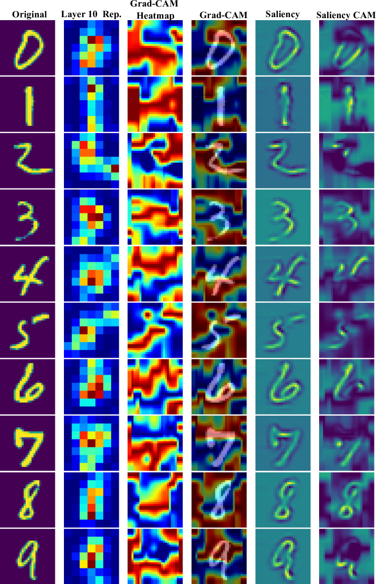
Figure 5: MNIST dataset original samples visualization. First column is the original/clean image sample. The second column is the representative output of the $10^{th}$ layer of baseline classifier. The third column is the heatmap generated with Grad-CAM technique. Fourth column is a combination of the heatmap and the corresponding original image. The fifth column is the Saliency map generated with Back-propagation technique while the last column is the combination of the saliency and the Grad-CAM heatmap.

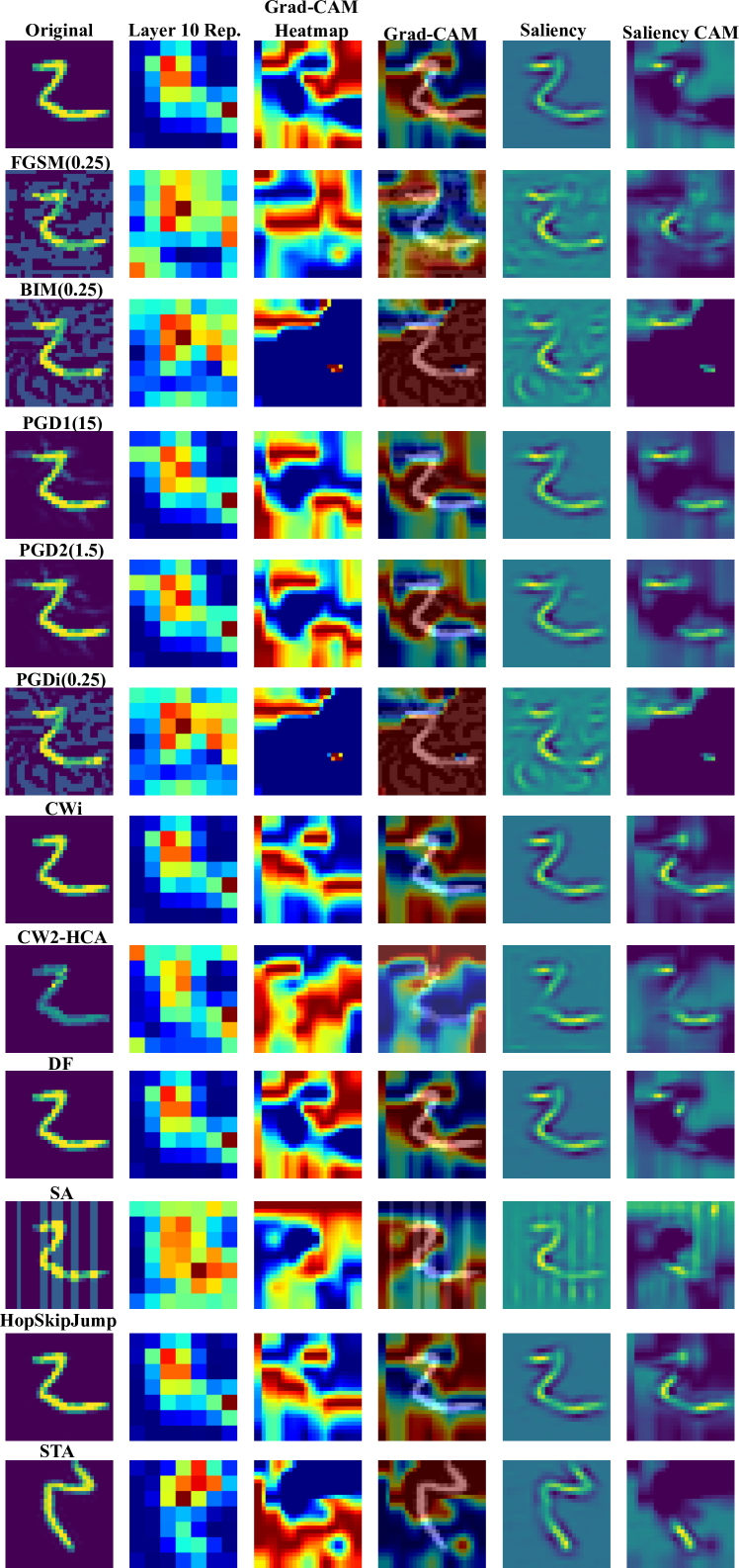
Figure 6: MNIST dataset original and adversarial samples visualization. First column is the original/clean or attacked image sample. The second column is the representative output of the $10^{th}$ layer of baseline classifier. The third column is the heatmap generated with Grad-CAM technique. Fourth column is a combination of the heatmap and the corresponding original or attacked image. The fifth column is the Saliency map generated with Back-propagation technique while the last column is the combination of the saliency and the Grad-CAM heatmap.

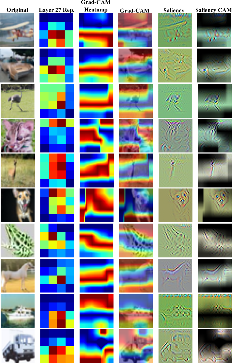
Figure 7: CIFAR dataset original samples visualization. First column is the original/clean image sample. The second column is the representative output of the $27^{th}$ layer of baseline classifier. The third column is the heatmap generated with Grad-CAM technique. Fourth column is a combination of the heatmap and the corresponding original image. The fifth column is the Saliency map generated with Back-propagation technique while the last column is the combination of the saliency and the Grad-CAM heatmap.

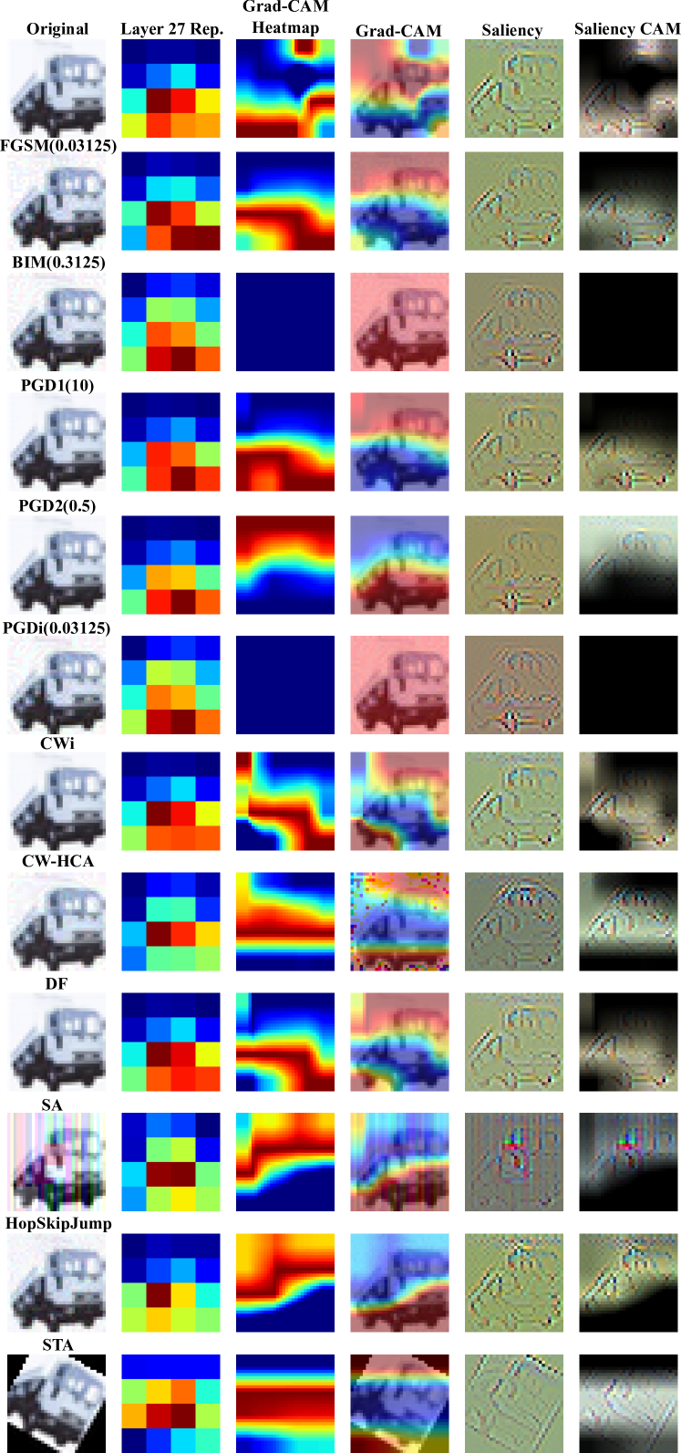
Figure 8: CIFAR dataset original and adversarial samples visualization. First column is the original/clean or attacked image sample. The second column is the representative output of the $27^{th}$ layer of baseline classifier. The third column is the heatmap generated with Grad-CAM technique. Fourth column is a combination of the heatmap and the corresponding original or attacked image. The fifth column is the Saliency map generated with Back-propagation technique while the last column is the combination of the saliency and the Grad-CAM heatmap.

7 Challenges, future perspectives, and conclusion

7.1 Challenges and future perspectives

The problem of adversarial examples is not yet solved. Figure 4 show that most of the detectors are not robust against new/unknown attacks. Moreover, findings from carlini2017adversarial ; athalye2018obfuscated show that the defenses and the detectors are vulnerable to the carefully designed adversarial perturbations. Hence, we can conclude that, to date, there are no robust defenses and detectors and more investigations are required to identify the features of the AEs. Such features will facilitate the design of robust defense and detection techniques. Moreover, researchers are facing many questions and challenges that are still open. Here we highlight them:

Supervised or Unsupervised detection? This is a confusing question. Supervised detection methods have, in general, better performance evaluation due to the detector capability to learn from labeled clean and AEs training data, but this is much restricted to known attacks and cannot be generalized to all kinds of attacks. Relatively, unsupervised detection method is much more flexible since it relies only on the clean data. The main two challenges of the unsupervised approach are 1) tuning its hyper-parameters is very challenging since it cannot be generalized to all models and datasets. 2) finding discriminating features for clean data that are not sensitive to noise and data processing like compression, for instance. As a recommendation, we need to focus on unsupervised detection methods. As discussed in Section 4, each unsupervised method proposed a way to detect the AEs and here is another confusing question, Which one to use? Denoiser based is much more effective if the denoiser has a good estimation of the training data and it does not require manual parameter tuning. Similar to denoiser based approaches, FS is highly dependent on the squeezer quality. These two approaches are not computationally expensive but have some inference test time latency. The statistical methods are effective in estimating training data distribution but it is not effective in large-scale applications with large amount of data and classes. It is time consuming in the training phase and has no inference test time latency. Most auxiliary models and NIC approaches depend on the underlying techniques and they require a lot of hyper-parameters tuning to be suitable for different DL based applications. Consequently, we leave the choice of the model to the application requirement.

Generalization. The wide view of generalization is the capability of the detector to detect white, black, gray (transferability) box attacks, and counter-counter attacks. The reported performance in Section 5 shows that we still need more research efforts to push detectors towards the generalization.

Lightweight detection. Lightweight detector is a detector that 1) has very small overhead, 2) has no inference time latency and 3) is not time consuming in training phase (some industries don’t care about that). According to the reported results of the reviewed detector, one of these factors is compromised. Thus, detectors that trade-off between these factors are highly recommended.

Ensemble Detection. It is believed that ensemble techniques can boost one detection technique. For instance,SFAD model used ensemble detection methods,selective/uncertainty prediction, softmax based predictionand bi-match prediction. These techniques are jointly integrated and give promised results with a little price to FPR. Hence, ensemble detection is highly recommended without compromising the FPR.

Meet the defense. As discussed in the Section 1, defense techniques, especially robust classification techniques, try to correctly classify input samples, whether attacked or not. Providing defense and detection jointly is an added value to the deployed model since it makes the adversary work much harder. In this approach, the adversary tries to generate AE with more perturbation to fool the defense, but in this case, it will be easy for the detector to detect it.

Training data Matters? Yes, the training data plays an important role. Firstly, not noisy training data helps a lot in understanding and recognizing AE features and properties in supervised and unsupervised detection methods. Secondly, findings in schmidt2018adversarially show that adversarially robust generalization requires more data. Hence, enough data helps in building CNN and detectors that generalize well. Finally, the designed CNN should be suitable and not complex with respect to the training data and the classification task.

Consider high resolution data. As discussed in Section 6.9, detectors face a huge challenge when they are tested on high resolution data such as ImageNet. They might be not effective, have high FPR, have high overhead, or/and are time consuming. Designing effective detectors for high resolution data is highly required.

7.2 Conclusion

This paper reviewed the detection methods of evasion attacks for neural networks classifiers of image classification task. We firstly categorized the AE detection methods into supervised and unsupervised methods. Then, each category is subdivided into statistical, auxiliary models, network invariant, feature squeezing, denoiser-based and object-based methods. Secondly, we demonstrated the performance evaluation of eight state-of-the-art algorithms experimentally in terms of detection rates, false positive rates, complexity, overhead and test time inference latency. We showed, as well, the impact of the content and the CNN with respect to detection methods. Finally, we highlighted the fact that the tested algorithms lack generalization and that more research efforts should be made in this research direction.

References

- [1] Alex Krizhevsky, Ilya Sutskever, and Geoffrey E Hinton. Imagenet classification with deep convolutional neural networks. In Advances in neural information processing systems, pages 1097–1105, 2012.
- [2] Karen Simonyan and Andrew Zisserman. Very deep convolutional networks for large-scale image recognition. In Yoshua Bengio and Yann LeCun, editors, 3rd International Conference on Learning Representations, ICLR 2015, San Diego, CA, USA, May 7-9, 2015, Conference Track Proceedings, 2015.
- [3] Shaoqing Ren, Kaiming He, Ross Girshick, and Jian Sun. Faster r-cnn: Towards real-time object detection with region proposal networks. In Advances in neural information processing systems, pages 91–99, 2015.
- [4] Jonathan Long, Evan Shelhamer, and Trevor Darrell. Fully convolutional networks for semantic segmentation. In Proceedings of the IEEE conference on computer vision and pattern recognition, pages 3431–3440, 2015.
- [5] Luca Bertinetto, Jack Valmadre, Joao F Henriques, Andrea Vedaldi, and Philip HS Torr. Fully-convolutional siamese networks for object tracking. In European conference on computer vision, pages 850–865. Springer, 2016.
- [6] Martin Danelljan, Goutam Bhat, Fahad Shahbaz Khan, and Michael Felsberg. Eco: Efficient convolution operators for tracking. In Proceedings of the IEEE conference on computer vision and pattern recognition, pages 6638–6646, 2017.
- [7] Justin Ker, Lipo Wang, Jai Rao, and Tchoyoson Lim. Deep learning applications in medical image analysis. IEEE Access, 6:9375–9389, 2017.
- [8] Dzmitry Bahdanau, Kyunghyun Cho, and Yoshua Bengio. Neural machine translation by jointly learning to align and translate. In Yoshua Bengio and Yann LeCun, editors, 3rd International Conference on Learning Representations, ICLR 2015, San Diego, CA, USA, May 7-9, 2015, Conference Track Proceedings, 2015.
- [9] Awni Y. Hannun, Carl Case, Jared Casper, Bryan Catanzaro, Greg Diamos, Erich Elsen, Ryan Prenger, Sanjeev Satheesh, Shubho Sengupta, Adam Coates, and Andrew Y. Ng. Deep speech: Scaling up end-to-end speech recognition. CoRR, abs/1412.5567, 2014.
- [10] Alexey Kurakin, Ian Goodfellow, and Samy Bengio. Adversarial examples in the physical world. ICLR Workshop, 2017.
- [11] Ivan Evtimov, Kevin Eykholt, Earlence Fernandes, Tadayoshi Kohno, Bo Li, Atul Prakash, Amir Rahmati, and Dawn Song. Robust physical-world attacks on machine learning models. CoRR, abs/1707.08945, 2017.
- [12] Tianyu Gu, Brendan Dolan-Gavitt, and Siddharth Garg. Badnets: Identifying vulnerabilities in the machine learning model supply chain. CoRR, abs/1708.06733, 2017.
- [13] Nicolas Papernot, Patrick McDaniel, Ian Goodfellow, Somesh Jha, Z Berkay Celik, and Ananthram Swami. Practical black-box attacks against machine learning. In Proceedings of the 2017 ACM on Asia conference on computer and communications security, pages 506–519, 2017.
- [14] Marco Melis, Ambra Demontis, Battista Biggio, Gavin Brown, Giorgio Fumera, and Fabio Roli. Is deep learning safe for robot vision? adversarial examples against the icub humanoid. In Proceedings of the IEEE International Conference on Computer Vision Workshops, pages 751–759, 2017.
- [15] Keiron O’Shea and Ryan Nash. An introduction to convolutional neural networks. arXiv preprint arXiv:1511.08458, 2015.
- [16] Kaiming He, Xiangyu Zhang, Shaoqing Ren, and Jian Sun. Deep residual learning for image recognition. In Proceedings of the IEEE conference on computer vision and pattern recognition, pages 770–778, 2016.
- [17] Christian Szegedy, Vincent Vanhoucke, Sergey Ioffe, Jonathon Shlens, and Zbigniew Wojna. Rethinking the inception architecture for computer vision. In 2016 IEEE Conference on Computer Vision and Pattern Recognition, CVPR 2016, Las Vegas, NV, USA, June 27-30, 2016, pages 2818–2826. IEEE Computer Society, 2016.
- [18] Andrew G. Howard, Menglong Zhu, Bo Chen, Dmitry Kalenichenko, Weijun Wang, Tobias Weyand, Marco Andreetto, and Hartwig Adam. Mobilenets: Efficient convolutional neural networks for mobile vision applications. CoRR, abs/1704.04861, 2017.
- [19] Yann LeCun, Léon Bottou, Yoshua Bengio, and Patrick Haffner. Gradient-based learning applied to document recognition. Proceedings of the IEEE, 86(11):2278–2324, 1998.
- [20] A. Krizhevsky and G. Hinton. Learning multiple layers of features from tiny images. Master’s thesis, Department of Computer Science, University of Toronto, 2009.
- [21] Yuval Netzer, Tao Wang, Adam Coates, Alessandro Bissacco, Bo Wu, and Andrew Y. Ng. Reading digits in natural images with unsupervised feature learning. In NIPS Workshop on Deep Learning and Unsupervised Feature Learning 2011, Granada, Spain, 2011.
- [22] Leon Yao and John Miller. Tiny imagenet classification with convolutional neural networks. CS 231N, 2(5):8, 2015.
- [23] J. Deng, W. Dong, R. Socher, L.-J. Li, K. Li, and L. Fei-Fei. ImageNet: A Large-Scale Hierarchical Image Database. In CVPR09, 2009.
- [24] Ross Girshick, Jeff Donahue, Trevor Darrell, and Jitendra Malik. Rich feature hierarchies for accurate object detection and semantic segmentation. In Proceedings of the IEEE conference on computer vision and pattern recognition, pages 580–587, 2014.
- [25] Ross B. Girshick. Fast R-CNN. In 2015 IEEE International Conference on Computer Vision, ICCV 2015, Santiago, Chile, December 7-13, 2015, pages 1440–1448. IEEE Computer Society, 2015.
- [26] Joseph Redmon, Santosh Kumar Divvala, Ross B. Girshick, and Ali Farhadi. You only look once: Unified, real-time object detection. In 2016 IEEE Conference on Computer Vision and Pattern Recognition, CVPR 2016, Las Vegas, NV, USA, June 27-30, 2016, pages 779–788. IEEE Computer Society, 2016.
- [27] Jacob Devlin, Ming-Wei Chang, Kenton Lee, and Kristina Toutanova. BERT: pre-training of deep bidirectional transformers for language understanding. In Proceedings of the 2019 Conference of the North American Chapter of the Association for Computational Linguistics: Human Language Technologies, NAACL-HLT 2019, Minneapolis, MN, USA, June 2-7, 2019, Volume 1 (Long and Short Papers), pages 4171–4186. Association for Computational Linguistics, 2019.
- [28] Zhilin Yang, Zihang Dai, Yiming Yang, Jaime G. Carbonell, Ruslan Salakhutdinov, and Quoc V. Le. Xlnet: Generalized autoregressive pretraining for language understanding. In Advances in Neural Information Processing Systems 32: Annual Conference on Neural Information Processing Systems 2019, NeurIPS 2019, December 8-14, 2019, Vancouver, BC, Canada, pages 5754–5764, 2019.
- [29] Zhenzhong Lan, Mingda Chen, Sebastian Goodman, Kevin Gimpel, Piyush Sharma, and Radu Soricut. ALBERT: A lite BERT for self-supervised learning of language representations. In 8th International Conference on Learning Representations, ICLR 2020, Addis Ababa, Ethiopia, April 26-30, 2020. OpenReview.net, 2020.
- [30] Nikolaos Pitropakis, Emmanouil Panaousis, Thanassis Giannetsos, Eleftherios Anastasiadis, and George Loukas. A taxonomy and survey of attacks against machine learning. Computer Science Review, 34:100199, 2019.
- [31] Yiming Li, Baoyuan Wu, Yong Jiang, Zhifeng Li, and Shu-Tao Xia. Backdoor learning: A survey. arXiv preprint arXiv:2007.08745, 2020.
- [32] Christian Szegedy, Wojciech Zaremba, Ilya Sutskever, Joan Bruna, Dumitru Erhan, Ian J. Goodfellow, and Rob Fergus. Intriguing properties of neural networks. In Yoshua Bengio and Yann LeCun, editors, 2nd International Conference on Learning Representations, ICLR 2014, Banff, AB, Canada, April 14-16, 2014, Conference Track Proceedings, 2014.
- [33] Nicholas Carlini and David Wagner. Adversarial examples are not easily detected: Bypassing ten detection methods. In Proceedings of the 10th ACM Workshop on Artificial Intelligence and Security, pages 3–14, 2017.
- [34] Andrew Ilyas, Shibani Santurkar, Dimitris Tsipras, Logan Engstrom, Brandon Tran, and Aleksander Madry. Adversarial examples are not bugs, they are features. In Advances in Neural Information Processing Systems, pages 125–136, 2019.
- [35] Naveed Akhtar and Ajmal Mian. Threat of adversarial attacks on deep learning in computer vision: A survey. IEEE Access, 6:14410–14430, 2018.
- [36] Han Xu Yao Ma Hao-Chen, Liu Debayan Deb, Hui Liu Ji-Liang Tang Anil, and K Jain. Adversarial attacks and defenses in images, graphs and text: A review. International Journal of Automation and Computing, 17(2):151–178, 2020.
- [37] Ian J. Goodfellow, Jonathon Shlens, and Christian Szegedy. Explaining and harnessing adversarial examples. In Yoshua Bengio and Yann LeCun, editors, 3rd International Conference on Learning Representations, ICLR 2015, San Diego, CA, USA, May 7-9, 2015, Conference Track Proceedings, 2015.
- [38] Seyed-Mohsen Moosavi-Dezfooli, Alhussein Fawzi, and Pascal Frossard. Deepfool: a simple and accurate method to fool deep neural networks. In Proceedings of the IEEE conference on computer vision and pattern recognition, pages 2574–2582, 2016.
- [39] Nicholas Carlini and David Wagner. Towards evaluating the robustness of neural networks. In 2017 ieee symposium on security and privacy (sp), pages 39–57. IEEE, 2017.
- [40] Aleksander Madry, Aleksandar Makelov, Ludwig Schmidt, Dimitris Tsipras, and Adrian Vladu. Towards deep learning models resistant to adversarial attacks. In 6th International Conference on Learning Representations, ICLR 2018, Vancouver, BC, Canada, April 30 - May 3, 2018, Conference Track Proceedings. OpenReview.net, 2018.
- [41] Nicolas Papernot, Patrick D. McDaniel, and Ian J. Goodfellow. Transferability in machine learning: from phenomena to black-box attacks using adversarial samples. CoRR, abs/1605.07277, 2016.
- [42] Pin-Yu Chen, Huan Zhang, Yash Sharma, Jinfeng Yi, and Cho-Jui Hsieh. Zoo: Zeroth order optimization based black-box attacks to deep neural networks without training substitute models. In Proceedings of the 10th ACM Workshop on Artificial Intelligence and Security, pages 15–26, 2017.
- [43] Logan Engstrom, Brandon Tran, Dimitris Tsipras, Ludwig Schmidt, and Aleksander Madry. Exploring the landscape of spatial robustness. In International Conference on Machine Learning, pages 1802–1811, 2019.
- [44] Jiawei Su, Danilo Vasconcellos Vargas, and Kouichi Sakurai. One pixel attack for fooling deep neural networks. IEEE Transactions on Evolutionary Computation, 23(5):828–841, 2019.
- [45] Shashank Kotyan and Danilo Vasconcellos Vargas. Adversarial robustness assessment: Why both and attacks are necessary. arXiv e-prints, pages arXiv–1906, 2019.
- [46] Cihang Xie, Jianyu Wang, Zhishuai Zhang, Yuyin Zhou, Lingxi Xie, and Alan L. Yuille. Adversarial examples for semantic segmentation and object detection. In IEEE International Conference on Computer Vision, ICCV 2017, Venice, Italy, October 22-29, 2017, pages 1378–1387. IEEE Computer Society, 2017.
- [47] Jiajun Lu, Hussein Sibai, Evan Fabry, and David A. Forsyth. NO need to worry about adversarial examples in object detection in autonomous vehicles. CoRR, abs/1707.03501, 2017.
- [48] Wei Emma Zhang, Quan Z Sheng, Ahoud Alhazmi, and Chenliang Li. Adversarial attacks on deep-learning models in natural language processing: A survey. ACM Transactions on Intelligent Systems and Technology (TIST), 11(3):1–41, 2020.
- [49] Lichao Sun, Kazuma Hashimoto, Wenpeng Yin, Akari Asai, Jia Li, Philip S. Yu, and Caiming Xiong. Adv-bert: BERT is not robust on misspellings! generating nature adversarial samples on BERT. CoRR, abs/2003.04985, 2020.
- [50] Di Li, Danilo Vasconcellos Vargas, and Kouichi Sakurai. Universal rules for fooling deep neural networks based text classification. In IEEE Congress on Evolutionary Computation, CEC 2019, Wellington, New Zealand, June 10-13, 2019, pages 2221–2228. IEEE, 2019.
- [51] Donghua Wang, Rangding Wang, Li Dong, Diqun Yan, Xueyuan Zhang, and Yongkang Gong. Adversarial examples attack and countermeasure for speech recognition system: A survey. In International Conference on Security and Privacy in Digital Economy, pages 443–468. Springer, 2020.
- [52] Huali Ren, Teng Huang, and Hongyang Yan. Adversarial examples: attacks and defenses in the physical world. International Journal of Machine Learning and Cybernetics, pages 1–12, 2021.
- [53] Prithviraj Dasgupta and Joseph Collins. A survey of game theoretic approaches for adversarial machine learning in cybersecurity tasks. AI Magazine, 40(2):31–43, 2019.
- [54] Samuel G. Finlayson, Isaac S. Kohane, and Andrew L. Beam. Adversarial attacks against medical deep learning systems. CoRR, abs/1804.05296, 2018.
- [55] Cihang Xie, Mingxing Tan, Boqing Gong, Alan L. Yuille, and Quoc V. Le. Smooth adversarial training. CoRR, abs/2006.14536, 2020.
- [56] Florian Tramèr, Alexey Kurakin, Nicolas Papernot, Ian J. Goodfellow, Dan Boneh, and Patrick D. McDaniel. Ensemble adversarial training: Attacks and defenses. In 6th International Conference on Learning Representations, ICLR 2018, Vancouver, BC, Canada, April 30 - May 3, 2018, Conference Track Proceedings. OpenReview.net, 2018.
- [57] Cihang Xie, Yuxin Wu, Laurens van der Maaten, Alan L Yuille, and Kaiming He. Feature denoising for improving adversarial robustness. In Proceedings of the IEEE Conference on Computer Vision and Pattern Recognition, pages 501–509, 2019.
- [58] Tejas Borkar, Felix Heide, and Lina Karam. Defending against universal attacks through selective feature regeneration. In Proceedings of the IEEE/CVF Conference on Computer Vision and Pattern Recognition, pages 709–719, 2020.
- [59] Fangzhou Liao, Ming Liang, Yinpeng Dong, Tianyu Pang, Xiaolin Hu, and Jun Zhu. Defense against adversarial attacks using high-level representation guided denoiser. In Proceedings of the IEEE Conference on Computer Vision and Pattern Recognition, pages 1778–1787, 2018.
- [60] Yassine Bakhti, Sid Ahmed Fezza, Wassim Hamidouche, and Olivier Déforges. Ddsa: a defense against adversarial attacks using deep denoising sparse autoencoder. IEEE Access, 7:160397–160407, 2019.
- [61] Aamir Mustafa, Salman H Khan, Munawar Hayat, Jianbing Shen, and Ling Shao. Image super-resolution as a defense against adversarial attacks. IEEE Transactions on Image Processing, 29:1711–1724, 2019.
- [62] Aaditya Prakash, Nick Moran, Solomon Garber, Antonella DiLillo, and James Storer. Deflecting adversarial attacks with pixel deflection. In Proceedings of the IEEE conference on computer vision and pattern recognition, pages 8571–8580, 2018.
- [63] Nicolas Papernot, Patrick McDaniel, Xi Wu, Somesh Jha, and Ananthram Swami. Distillation as a defense to adversarial perturbations against deep neural networks. In 2016 IEEE Symposium on Security and Privacy (SP), pages 582–597. IEEE, 2016.
- [64] Shixiang Gu and Luca Rigazio. Towards deep neural network architectures robust to adversarial examples. In Yoshua Bengio and Yann LeCun, editors, 3rd International Conference on Learning Representations, ICLR 2015, San Diego, CA, USA, May 7-9, 2015, Workshop Track Proceedings, 2015.
- [65] Aran Nayebi and Surya Ganguli. Biologically inspired protection of deep networks from adversarial attacks. CoRR, abs/1703.09202, 2017.
- [66] Kathrin Grosse, Praveen Manoharan, Nicolas Papernot, Michael Backes, and Patrick D. McDaniel. On the (statistical) detection of adversarial examples. CoRR, abs/1702.06280, 2017.
- [67] Dongyu Meng and Hao Chen. Magnet: a two-pronged defense against adversarial examples. In Proceedings of the 2017 ACM SIGSAC conference on computer and communications security, pages 135–147, 2017.
- [68] Weilin Xu, David Evans, and Yanjun Qi. Feature squeezing: Detecting adversarial examples in deep neural networks. In 25th Annual Network and Distributed System Security Symposium, NDSS 2018, San Diego, California, USA, February 18-21, 2018. The Internet Society, 2018.
- [69] Kathrin Grosse, Nicolas Papernot, Praveen Manoharan, Michael Backes, and Patrick D. McDaniel. Adversarial perturbations against deep neural networks for malware classification. CoRR, abs/1606.04435, 2016.
- [70] Shiqing Ma and Yingqi Liu. Nic: Detecting adversarial samples with neural network invariant checking. In Proceedings of the 26th Network and Distributed System Security Symposium (NDSS 2019), 2019.
- [71] Guillermo Ortiz-Jiménez, Apostolos Modas, Seyed-Mohsen Moosavi-Dezfooli, and Pascal Frossard. Optimism in the face of adversity: Understanding and improving deep learning through adversarial robustness. Proceedings of the IEEE, 109(5):635–659, 2021.
- [72] Xiaoyong Yuan, Pan He, Qile Zhu, and Xiaolin Li. Adversarial examples: Attacks and defenses for deep learning. IEEE transactions on neural networks and learning systems, 30(9):2805–2824, 2019.
- [73] Anirban Chakraborty, Manaar Alam, Vishal Dey, Anupam Chattopadhyay, and Debdeep Mukhopadhyay. Adversarial attacks and defences: A survey. CoRR, abs/1810.00069, 2018.
- [74] Xianmin Wang, Jing Li, Xiaohui Kuang, Yu-an Tan, and Jin Li. The security of machine learning in an adversarial setting: A survey. Journal of Parallel and Distributed Computing, 130:12–23, 2019.
- [75] Gabriel Resende Machado, Eugênio Silva, and Ronaldo Ribeiro Goldschmidt. Adversarial machine learning in image classification: A survey towards the defender’s perspective. CoRR, abs/2009.03728, 2020.
- [76] Saikiran Bulusu, Bhavya Kailkhura, Bo Li, Pramod K Varshney, and Dawn Song. Anomalous example detection in deep learning: A survey. IEEE Access, 8:132330–132347, 2020.
- [77] David Miller, Yujia Wang, and George Kesidis. When not to classify: Anomaly detection of attacks (ada) on dnn classifiers at test time. Neural computation, 31(8):1624–1670, 2019.
- [78] David J Miller, Zhen Xiang, and George Kesidis. Adversarial learning targeting deep neural network classification: A comprehensive review of defenses against attacks. Proceedings of the IEEE, 108(3):402–433, 2020.
- [79] Alex Serban, Erik Poll, and Joost Visser. Adversarial examples on object recognition: A comprehensive survey. ACM Computing Surveys (CSUR), 53(3):1–38, 2020.
- [80] Battista Biggio, Igino Corona, Davide Maiorca, Blaine Nelson, Nedim Šrndić, Pavel Laskov, Giorgio Giacinto, and Fabio Roli. Evasion attacks against machine learning at test time. In Joint European conference on machine learning and knowledge discovery in databases, pages 387–402. Springer, 2013.
- [81] Yanpei Liu, Xinyun Chen, Chang Liu, and Dawn Song. Delving into transferable adversarial examples and black-box attacks. In 5th International Conference on Learning Representations, ICLR 2017, Toulon, France, April 24-26, 2017, Conference Track Proceedings. OpenReview.net, 2017.
- [82] Battista Biggio, Giorgio Fumera, and Fabio Roli. Pattern recognition systems under attack: Design issues and research challenges. International Journal of Pattern Recognition and Artificial Intelligence, 28(07):1460002, 2014.
- [83] Battista Biggio, Igino Corona, Blaine Nelson, Benjamin IP Rubinstein, Davide Maiorca, Giorgio Fumera, Giorgio Giacinto, and Fabio Roli. Security evaluation of support vector machines in adversarial environments. In Support Vector Machines Applications, pages 105–153. Springer, 2014.
- [84] Battista Biggio and Fabio Roli. Wild patterns: Ten years after the rise of adversarial machine learning. Pattern Recognition, 84:317–331, 2018.
- [85] Dong C Liu and Jorge Nocedal. On the limited memory bfgs method for large scale optimization. Mathematical programming, 45(1-3):503–528, 1989.
- [86] Francesco Croce and Matthias Hein. Reliable evaluation of adversarial robustness with an ensemble of diverse parameter-free attacks. In Proceedings of the 37th International Conference on Machine Learning, ICML 2020, 13-18 July 2020, Virtual Event, volume 119 of Proceedings of Machine Learning Research, pages 2206–2216. PMLR, 2020.
- [87] Seyed-Mohsen Moosavi-Dezfooli, Alhussein Fawzi, Omar Fawzi, and Pascal Frossard. Universal adversarial perturbations. In Proceedings of the IEEE conference on computer vision and pattern recognition, pages 1765–1773, 2017.
- [88] Nicolas Papernot, Patrick McDaniel, Somesh Jha, Matt Fredrikson, Z Berkay Celik, and Ananthram Swami. The limitations of deep learning in adversarial settings. In 2016 IEEE European symposium on security and privacy (EuroS&P), pages 372–387. IEEE, 2016.
- [89] Sara Sabour, Yanshuai Cao, Fartash Faghri, and David J. Fleet. Adversarial manipulation of deep representations. In Yoshua Bengio and Yann LeCun, editors, 4th International Conference on Learning Representations, ICLR 2016, San Juan, Puerto Rico, May 2-4, 2016, Conference Track Proceedings, 2016.
- [90] Shumeet Baluja and Ian Fischer. Adversarial transformation networks: Learning to generate adversarial examples. CoRR, abs/1703.09387, 2017.
- [91] Anish Athalye, Logan Engstrom, Andrew Ilyas, and Kevin Kwok. Synthesizing robust adversarial examples. In International conference on machine learning, pages 284–293. PMLR, 2018.
- [92] Anish Athalye, Nicholas Carlini, and David A. Wagner. Obfuscated gradients give a false sense of security: Circumventing defenses to adversarial examples. In Jennifer G. Dy and Andreas Krause, editors, Proceedings of the 35th International Conference on Machine Learning, ICML 2018, Stockholmsmässan, Stockholm, Sweden, July 10-15, 2018, volume 80 of Proceedings of Machine Learning Research, pages 274–283. PMLR, 2018.
- [93] Maksym Andriushchenko, Francesco Croce, Nicolas Flammarion, and Matthias Hein. Square attack: A query-efficient black-box adversarial attack via random search. In Andrea Vedaldi, Horst Bischof, Thomas Brox, and Jan-Michael Frahm, editors, Computer Vision - ECCV 2020 - 16th European Conference, Glasgow, UK, August 23-28, 2020, Proceedings, Part XXIII, volume 12368 of Lecture Notes in Computer Science, pages 484–501. Springer, 2020.
- [94] Wieland Brendel, Jonas Rauber, and Matthias Bethge. Decision-based adversarial attacks: Reliable attacks against black-box machine learning models. In 6th International Conference on Learning Representations, ICLR 2018, Vancouver, BC, Canada, April 30 - May 3, 2018, Conference Track Proceedings. OpenReview.net, 2018.
- [95] Jianbo Chen, Michael I Jordan, and Martin J Wainwright. Hopskipjumpattack: A query-efficient decision-based attack. In 2020 ieee symposium on security and privacy (sp), pages 1277–1294. IEEE, 2020.
- [96] Sayantan Sarkar, Ankan Bansal, Upal Mahbub, and Rama Chellappa. UPSET and ANGRI : Breaking high performance image classifiers. CoRR, abs/1707.01159, 2017.
- [97] Anh Nguyen, Jason Yosinski, and Jeff Clune. Deep neural networks are easily fooled: High confidence predictions for unrecognizable images. In Proceedings of the IEEE conference on computer vision and pattern recognition, pages 427–436, 2015.
- [98] Nicholas Carlini and David A. Wagner. Defensive distillation is not robust to adversarial examples. CoRR, abs/1607.04311, 2016.
- [99] Jiajun Lu, Theerasit Issaranon, and David Forsyth. Safetynet: Detecting and rejecting adversarial examples robustly. In Proceedings of the IEEE International Conference on Computer Vision, pages 446–454, 2017.
- [100] Stefanos Pertigkiozoglou and Petros Maragos. Detecting adversarial examples in convolutional neural networks. CoRR, abs/1812.03303, 2018.
- [101] Fabio Carrara, Rudy Becarelli, Roberto Caldelli, Fabrizio Falchi, and Giuseppe Amato. Adversarial examples detection in features distance spaces. In Proceedings of the European Conference on Computer Vision (ECCV), pages 0–0, 2018.
- [102] Jan Hendrik Metzen, Tim Genewein, Volker Fischer, and Bastian Bischoff. On detecting adversarial perturbations. In 5th International Conference on Learning Representations, ICLR 2017, Toulon, France, April 24-26, 2017, Conference Track Proceedings. OpenReview.net, 2017.
- [103] Hasan Ferit Eniser, Maria Christakis, and Valentin Wüstholz. RAID: randomized adversarial-input detection for neural networks. CoRR, abs/2002.02776, 2020.
- [104] Reuben Feinman, Ryan R. Curtin, Saurabh Shintre, and Andrew B. Gardner. Detecting adversarial samples from artifacts. CoRR, abs/1703.00410, 2017.
- [105] Lewis Smith and Yarin Gal. Understanding measures of uncertainty for adversarial example detection. In Amir Globerson and Ricardo Silva, editors, Proceedings of the Thirty-Fourth Conference on Uncertainty in Artificial Intelligence, UAI 2018, Monterey, California, USA, August 6-10, 2018, pages 560–569. AUAI Press, 2018.
- [106] Dan Hendrycks and Kevin Gimpel. A baseline for detecting misclassified and out-of-distribution examples in neural networks. In 5th International Conference on Learning Representations, ICLR 2017, Toulon, France, April 24-26, 2017, Conference Track Proceedings. OpenReview.net, 2017.
- [107] Jonathan Aigrain and Marcin Detyniecki. Detecting adversarial examples and other misclassifications in neural networks by introspection. CoRR, abs/1905.09186, 2019.
- [108] João Monteiro, Isabela Albuquerque, Zahid Akhtar, and Tiago H Falk. Generalizable adversarial examples detection based on bi-model decision mismatch. In 2019 IEEE International Conference on Systems, Man and Cybernetics (SMC), pages 2839–2844. IEEE, 2019.
- [109] Zhitao Gong, Wenlu Wang, and Wei-Shinn Ku. Adversarial and clean data are not twins. CoRR, abs/1704.04960, 2017.
- [110] Hossein Hosseini, Yize Chen, Sreeram Kannan, Baosen Zhang, and Radha Poovendran. Blocking transferability of adversarial examples in black-box learning systems. CoRR, abs/1703.04318, 2017.
- [111] Julia Lust and Alexandru Paul Condurache. Gran: An efficient gradient-norm based detector for adversarial and misclassified examples. In 28th European Symposium on Artificial Neural Networks, Computational Intelligence and Machine Learning, ESANN 2020, Bruges, Belgium, October 2-4, 2020, pages 7–12, 2020.
- [112] Anouar Kherchouche, Sid Ahmed Fezza, Wassim Hamidouche, and Olivier Déforges. Detection of adversarial examples in deep neural networks with natural scene statistics. In 2020 International Joint Conference on Neural Networks (IJCNN), pages 1–7. IEEE, 2020.
- [113] Fei Zuo and Qiang Zeng. Exploiting the sensitivity of L2 adversarial examples to erase-and-restore. In Jiannong Cao, Man Ho Au, Zhiqiang Lin, and Moti Yung, editors, ASIA CCS ’21: ACM Asia Conference on Computer and Communications Security, Virtual Event, Hong Kong, June 7-11, 2021, pages 40–51. ACM, 2021.
- [114] Xin Li and Fuxin Li. Adversarial examples detection in deep networks with convolutional filter statistics. In Proceedings of the IEEE International Conference on Computer Vision, pages 5764–5772, 2017.
- [115] Xingjun Ma, Bo Li, Yisen Wang, Sarah M. Erfani, Sudanthi N. R. Wijewickrema, Grant Schoenebeck, Dawn Song, Michael E. Houle, and James Bailey. Characterizing adversarial subspaces using local intrinsic dimensionality. In 6th International Conference on Learning Representations, ICLR 2018, Vancouver, BC, Canada, April 30 - May 3, 2018, Conference Track Proceedings. OpenReview.net, 2018.
- [116] Gilad Cohen, Guillermo Sapiro, and Raja Giryes. Detecting adversarial samples using influence functions and nearest neighbors. In Proceedings of the IEEE/CVF Conference on Computer Vision and Pattern Recognition, pages 14453–14462, 2020.
- [117] Kimin Lee, Kibok Lee, Honglak Lee, and Jinwoo Shin. A simple unified framework for detecting out-of-distribution samples and adversarial attacks. In Advances in Neural Information Processing Systems, pages 7167–7177, 2018.
- [118] Scott Freitas, Shang-Tse Chen, Zijie J. Wang, and Duen Horng Chau. Unmask: Adversarial detection and defense through robust feature alignment. In IEEE International Conference on Big Data, Big Data 2020, Atlanta, GA, USA, December 10-13, 2020, pages 1081–1088. IEEE, 2020.
- [119] Yang Song, Taesup Kim, Sebastian Nowozin, Stefano Ermon, and Nate Kushman. Pixeldefend: Leveraging generative models to understand and defend against adversarial examples. In 6th International Conference on Learning Representations, ICLR 2018, Vancouver, BC, Canada, April 30 - May 3, 2018, Conference Track Proceedings. OpenReview.net, 2018.
- [120] Dan Hendrycks and Kevin Gimpel. Early methods for detecting adversarial images. In 5th International Conference on Learning Representations, ICLR 2017, Toulon, France, April 24-26, 2017, Workshop Track Proceedings. OpenReview.net, 2017.
- [121] Zhihao Zheng and Pengyu Hong. Robust detection of adversarial attacks by modeling the intrinsic properties of deep neural networks. In Advances in Neural Information Processing Systems, pages 7913–7922, 2018.
- [122] Bin Liang, Hongcheng Li, Miaoqiang Su, Xirong Li, Wenchang Shi, and Xiaofeng Wang. Detecting adversarial image examples in deep neural networks with adaptive noise reduction. IEEE Trans. Dependable Secur. Comput., 18(1):72–85, 2021.
- [123] Fabio Carrara, Fabrizio Falchi, Roberto Caldelli, Giuseppe Amato, Roberta Fumarola, and Rudy Becarelli. Detecting adversarial example attacks to deep neural networks. In Proceedings of the 15th International Workshop on Content-Based Multimedia Indexing, pages 1–7, 2017.
- [124] Tianyu Pang, Chao Du, Yinpeng Dong, and Jun Zhu. Towards robust detection of adversarial examples. In Advances in Neural Information Processing Systems, pages 4579–4589, 2018.
- [125] Fatemeh Sheikholeslami, Swayambhoo Jain, and Georgios B. Giannakis. Minimum uncertainty based detection of adversaries in deep neural networks. In Information Theory and Applications Workshop, ITA 2020, San Diego, CA, USA, February 2-7, 2020, pages 1–16. IEEE, 2020.
- [126] Angelo Sotgiu, Ambra Demontis, Marco Melis, Battista Biggio, Giorgio Fumera, Xiaoyi Feng, and Fabio Roli. Deep neural rejection against adversarial examples. EURASIP Journal on Information Security, 2020:1–10, 2020.
- [127] Ahmed Aldahdooh, Wassim Hamidouche, and Olivier Déforges. Revisiting model’s uncertainty and confidences for adversarial example detection. arXiv preprint arXiv:2103.05354, 2021.
- [128] Nicholas Carlini and David A. Wagner. Magnet and ”efficient defenses against adversarial attacks” are not robust to adversarial examples. CoRR, abs/1711.08478, 2017.
- [129] Nitish Srivastava, Geoffrey Hinton, Alex Krizhevsky, Ilya Sutskever, and Ruslan Salakhutdinov. Dropout: a simple way to prevent neural networks from overfitting. The journal of machine learning research, 15(1):1929–1958, 2014.
- [130] Christian Szegedy, Vincent Vanhoucke, Sergey Ioffe, Jonathon Shlens, and Zbigniew Wojna. Rethinking the inception architecture for computer vision. 2015. arXiv preprint arXiv:1512.00567, 2015.
- [131] Anish Mittal, Anush Krishna Moorthy, and Alan Conrad Bovik. No-reference image quality assessment in the spatial domain. IEEE Transactions on image processing, 21(12):4695–4708, 2012.
- [132] Arthur Gretton, Karsten M Borgwardt, Malte J Rasch, Bernhard Schölkopf, and Alexander Smola. A kernel two-sample test. The Journal of Machine Learning Research, 13(1):723–773, 2012.
- [133] Xiaofeng Mao, Yuefeng Chen, Yuhong Li, Yuan He, and Hui Xue. Learning to characterize adversarial subspaces. In ICASSP 2020-2020 IEEE International Conference on Acoustics, Speech and Signal Processing (ICASSP), pages 2438–2442. IEEE, 2020.
- [134] Ashish Vaswani, Noam Shazeer, Niki Parmar, Jakob Uszkoreit, Llion Jones, Aidan N. Gomez, Lukasz Kaiser, and Illia Polosukhin. Attention is all you need. In Advances in Neural Information Processing Systems 30: Annual Conference on Neural Information Processing Systems 2017, December 4-9, 2017, Long Beach, CA, USA, pages 5998–6008, 2017.
- [135] Yonatan Geifman and Ran El-Yaniv. Selectivenet: A deep neural network with an integrated reject option. CoRR, abs/1901.09192, 2019.
- [136] Solomon Kullback and Richard A Leibler. On information and sufficiency. The annals of mathematical statistics, 22(1):79–86, 1951.
- [137] Aaron Van den Oord, Nal Kalchbrenner, Lasse Espeholt, Oriol Vinyals, Alex Graves, et al. Conditional image generation with pixelcnn decoders. Advances in neural information processing systems, 29:4790–4798, 2016.
- [138] Gao Huang, Zhuang Liu, Laurens Van Der Maaten, and Kilian Q Weinberger. Densely connected convolutional networks. In Proceedings of the IEEE conference on computer vision and pattern recognition, pages 4700–4708, 2017.
- [139] Maria-Irina Nicolae, Mathieu Sinn, Minh Ngoc Tran, Beat Buesser, Ambrish Rawat, Martin Wistuba, Valentina Zantedeschi, Nathalie Baracaldo, Bryant Chen, Heiko Ludwig, Ian M. Molloy, and Ben Edwards. Adversarial robustness toolbox v1.0.0, 2019.
- [140] Kaiming He, Xiangyu Zhang, Shaoqing Ren, and Jian Sun. Identity mappings in deep residual networks. In European conference on computer vision, pages 630–645. Springer, 2016.
- [141] Ramprasaath R. Selvaraju, Michael Cogswell, Abhishek Das, Ramakrishna Vedantam, Devi Parikh, and Dhruv Batra. Grad-cam: Visual explanations from deep networks via gradient-based localization. In IEEE International Conference on Computer Vision, ICCV 2017, Venice, Italy, October 22-29, 2017, pages 618–626. IEEE Computer Society, 2017.
- [142] Jost Tobias Springenberg, Alexey Dosovitskiy, Thomas Brox, and Martin A. Riedmiller. Striving for simplicity: The all convolutional net. In Yoshua Bengio and Yann LeCun, editors, 3rd International Conference on Learning Representations, ICLR 2015, San Diego, CA, USA, May 7-9, 2015, Workshop Track Proceedings, 2015.
- [143] Ludwig Schmidt, Shibani Santurkar, Dimitris Tsipras, Kunal Talwar, and Aleksander Madry. Adversarially robust generalization requires more data. In Advances in Neural Information Processing Systems 31: Annual Conference on Neural Information Processing Systems 2018, NeurIPS 2018, December 3-8, 2018, Montréal, Canada, pages 5019–5031, 2018.