On a nodal observer for a semilinear model for the flow in gas networks

Abstract

The flow of gas through networks of pipes can be modeled by coupling hyperbolic systems of partial differential equations that describe the flow through the pipes that form the edges of the graph of the network by algebraic node conditions that model the flow through the vertices of the graph. In the network, measurements of the state are available at certain points in space. Based upon these nodal observations, the complete system state can be approximated using an observer system. In this paper we present a nodal observer, and prove that the state of the observer system converges to the original state exponentially fast. Numerical experiments confirm the theoretical findings.

This work was supported by DFG in the framework of the Collaborative Research Centre CRC/Transregio 154, Mathematical Modelling, Simulation and Optimization Using the Example of Gas Networks, Project C03 and Project C05.

Introduction

In this contribution we study the problem to construct an observer for the flow of gas through networks of pipelines. In this application, in general, many pipelines are very long and the graph of the network can be quite complex. We consider a semilinear model for a gas pipeline network where at the nodes the solutions for the adjacent pipes are coupled by algebraic node conditions that require the conservation of mass and the continuity of the pressure. The semilinear model is a resonable simplification of the quasilinear isothermal Euler equations if the Mach number of the flow is quite small. In the operation of gas transportation systems this is the case, since the velocity of the gas flow is much smaller than the sound speed. The eigenvalues of the quasilinear system have the form $c+v$ and $-c+v$, where $v$ denotes the velocity of the gas and $c$ denotes the sound speed. In order to obtain a semilinear model the eigenvalues are replaced by the sound speed, that is by $-c$ and $c$, at some reference density. While we linearize the convection, in our semilinear model we keep the nonlinear source term. This source term plays an essential role in the model of gas network flow, since the friction effects lead to a decrease of the pressure along each pipe in the direction of the flow.

In this paper, we present a nodal observer system for the network flow where the coupling to the original system is governed at each vertex $v$ by a parameter $\mu^{v}\in[-1,1]$. We show that the observer system yields an approximation of the state in the original system where the error decays exponentially fast in the sense of the $L^{2}$-norm if the $L^{\infty}$-norm of the initial state is sufficiently small. Moreover, we also show that the $H^{1}$-norm of the approximation error decays exponentially fast if the state of the original system is sufficiently regular (i.e. in $W^{1,\infty}$). It is desirable to have such an observer since it allows to obtain a reliable approximation for the complete state in the original system. The state estimation that is obtained with the observer system can be used in the construction of feedback laws. The proofs are based upon nodal observability inequalities for the flow.

Observers, using distributed measurements, have been constructed for semi-linear hyperbolic equations [6, 7] and quasi-linear hyperbolic equations [1]. The results for semi-linear hyperbolic equations are based on stabilization results for (locally) damped wave equations [17]. The result for quasi-linear problems is based on a kinetic formulation and, thus, uses a rather different approach. In [18] the backstepping method has been used to construct a boundary observer for semi-linear hyperbolic problems. For results about the recovery of an unknown initial state using an observer see [20]. In [10], the design of boundary observers for a linear system of ODEs in cascade with hyperbolic PDEs is studied and more references on observer design are given. We want to emphasize that the novelty of our contribution is the construction of an observer for a system that is governed by networked semilinear pdes and uses observations that are located pointwise in space, whereas in the previous contributions distributed observations coming from subdomains in space have been considered.

This paper has the following structure. In Section 1.1 we introduce the quasilinear isothermal Euler equations. In Section 1.2, we present the corresponding Riemann invariants and transform the system in diagonal form. In Section 2 we present the node conditions that model the flow through the junctions in a gas pipeline network. Then we derive the semilinear model that provides an approximation for small gas velocities.

We are working in the framework of solutions that are defined through a fixed point iteration along the characteristics. The definition of the fixed point mapping is derived from the integral equations along the characteristic curves that are known a priori for the semilinear model. A well–posedness result that is based on this approach is presented in Section 3.

In Section 6 we show that the error of the observer converges to zero in $L^{2}$ exponentially fast. For the proof, in Section 4 we first introduce a quadratic $L^{2}$-Lyapunov function and show that it decays exponentially fast on finite time intervals without additional constraints on the lengths of the pipes. In the proof we use an observability inequality for the $L^{2}$-norm. Then in Section 5 we define a quadratic Lyapunov function with exponential weights to show that the time derivatives also decay exponentially fast. This yields the exponential decay of the $H^{1}$-norm of the state for initial states with sufficiently small $H^{1}$-norm. This is also shown in Section 6. However, the result about the exponential decay in $H^{1}$ requires strict bounds on the lengths of the pipes. In Section 7 at the end of the paper, numerical results are presented.

1 Motivating the semilinear model from the Euler equations

1.1 The isothermal Euler equations along the pipes

The isothermal Euler equations as a model for the flow through gas pipelines have been stated for example in [3]. Let a finite graph $G=(V,\,E)$ of a pipeline network be given. Here $V$ denotes the set of vertices and $E$ denotes the set of edges. Each edge $e\in E$ corresponds to an interval $[0,\,L^{e}]$ that represents a pipe of length $L^{e}>0$. Let $D^{e}>0$ denote the diameter and $\lambda_{fric}^{e}>0$ the friction coefficient in pipe $e$. Define $\theta^{e}=\frac{\lambda_{fric}^{e}}{D^{e}}$. Let $\rho^{e}$ denote the gas density, $p^{e}$ the pressure and $q^{e}$ the mass flow rate. Since we will linearize the convective part of the equations, we will not specify any pressure law. The isothermal or isentropic Euler equations are hyperbolic provided the pressure $p=p(\rho)$ is given as a monotone increasing function of the density. We will assume that this monotonicity is strict. Typical examples are isentropic law $p(\rho)=a\rho^{\gamma}$ with $a>0$ and $\gamma>1$ and the model of the American Gas Association (AGA), see [15],

$$p(\rho)=\frac{R_{s}T\rho}{1-\tilde{\alpha}\rho}$$

where $T$ is the temperature of the pipe, $R_{s}$ is the gas constant and $\tilde{\alpha}\leqslant 0$. Note that for $\tilde{\alpha}=0$ the AGA model reduces to the isothermal law $p(\rho)=R_{s}T\rho$. We study a model that is based upon the $2$ Euler equations, i.e. there is no energy conservation equation,

$$\left\{\begin{array}[]{l}\rho_{t}^{e}+q_{x}^{e}=0,\\ q_{t}^{e}+\left(p^{e}+\frac{(q^{e})^{2}}{\rho^{e}}\right)_{x}=-\frac{1}{2}\theta^{e}\frac{q^{e}\;|q^{e}|}{\rho^{e}}\end{array}\right.$$ (1)

that govern the flow through pipe $e$. In order to deal with large networks, it is desirable to replace the quasilinear Euler equations by a simpler semilinear model. In the sequel, we will present such a model. We proceed in the following way. First we transform the system to a system in diagonal form for the Riemann invariants. Then we observe that in the normal operational of range gas pipeline flow (that is for slow transients), the matrix in the diagonal form is close to a constant matrix. We obtain a semilinear model by replacing the system matrix by this constant matrix.

1.2 The system in terms of Riemann invariants

Hyperbolic systems of conservation laws can be diagonalized by Riemann invariants, i.e. quantities whose derivatives with respect to the conserved variables are orthogonal to all but one of the left eigenvectors of the Jacobian of the flux.

Here the flux, its Jacobian, and the eigenvectors are given by

$$f(\rho,q)=\begin{pmatrix}q\\ \frac{q^{2}}{\rho}+p\end{pmatrix},\ Df(\rho,q)=\begin{pmatrix}0&1\\ -\frac{q^{2}}{\rho^{2}}+p^{\prime}(\rho)&2\frac{q}{\rho}\end{pmatrix},\ \ell_{\pm}(\rho,q)=\begin{pmatrix}-1\\ \frac{q}{\rho}\pm\sqrt{p^{\prime}(\rho)}.\end{pmatrix}$$

As explained in [8, Chapter 7.3] every $2\times 2$ system of hyperbolic conservation laws is endowed with a system of Riemann invariants. For the Euler equations with general pressure law they are given by

$$R_{\pm}(\rho,q)=\tilde{R}(\rho)\pm\frac{q}{\rho}$$

where $\tilde{R}$ is defined by $\tilde{R}(\rho)=\int_{1}^{\rho}\frac{\sqrt{p^{\prime}(r)}}{r}\,dr.$ Specific formulas for Riemann invariants for the isentropic law $p(\rho)=a\rho^{\gamma}$ can be found in [8, Chapter 7.3] while the specific formulas for the AGA model was computed in [15]. Note that Riemann invariants are only unique up operations that leave the direction of the gradient unchanged.

2 The Node Conditions for the Network Flow

In this section we introduce the coupling conditions that model the flow through the nodes of the network. For any node $v\in V$ let $E_{0}(v)$ denote the set of edges in the graph that are incident to $v\in V$ and let $x^{e}(v)\in\{0,L^{e}\}$ denote the end of the interval $[0,L^{e}]$ that corresponds to the edge $e$ that is adjacent to $v$. Let $V_{0}(e)$ denote the set of nodes adjacent to some edge $e$. Define

$${\mathfrak{s}}(v,\,e):=\left\{\begin{array}[]{rll}-1&{\rm if}&x^{e}(v)=0\;\mbox{\rm and }\;e\in E_{0}(v),\\ 1&{\rm if}&x^{e}(v)=L^{e}\;\mbox{\rm and }\;e\in E_{0}(v),\\ 0&{\rm if}&e\not\in E_{0}(v).\end{array}\right.$$ (2)

We impose the Kirchhoff condition

$$\sum_{e\in E_{0}(v)}{\mathfrak{s}}(v,\,e)\,(D^{e})^{2}\,q^{e}(x^{e}(v))=0$$ (3)

that expresses conservation of mass at the nodes.

In order to close the system, additional coupling conditions are needed . A typical choice, leading to well-posed Riemann problems [3], is to require the continuity of the pressure at $v$, which means that for all $e$, $f\in E_{0}(v)$ we have

$$p(\rho^{e}(t,x^{e}(v)))=p(\rho^{f}(t,x^{f}(v))).$$ (4)

another choice, which was advocated by [23] is continuity of enthalpy: for all $e$, $f\in E_{0}(v)$ we have

$$P^{\prime}(\rho^{e}(t,x^{e}(v)))+\frac{(q^{e}(t,x^{e}(v))^{2}}{(\rho^{e}(t,x^{e}(v))^{2}}=P^{\prime}(\rho^{e}(t,x^{f}(v)))+\frac{(q^{f}(t,x^{e}(v))^{2}}{(\rho^{f}(t,x^{e}(v))^{2}}$$ (5)

where $P=P(\rho)$ is the pressure potential that is defined by

$$P(\rho)=\rho\int_{1}^{\rho}\frac{p(r)}{r^{2}}dr,$$ (6)

Our interest is in simplified models where velocities are much smaller than the speed of sound. Let us note that in the $\tfrac{q}{\rho}\rightarrow 0$ limit both (4) and (5) enforce continuity of densities, since $p(\rho)$ and $P^{\prime}(\rho)$ are both strictly monotone increasing. Since both conditions coincide (asymptotically) in the limit of interest, we will use (4) for our further discussions, irrespective of the question of which coupling is correct for general flows.

Now also state the node conditions in terms of Riemann invariants.

Define the vectors $R_{in}^{v}(t)$, $R_{out}^{v}(t)\in{\mathbb{R}}^{|E_{0}(v)|}$ in the following manner:
If $e\in E_{0}(v)$ and ${\mathfrak{s}}(v,\,e)=1$, $R^{e}_{+}(t,\,x^{e}(v))$ is a component of $R_{in}^{v}(t)$ that we refer to as $R_{in}^{e}(t,x^{e}(v))$ and if $e\in E_{0}(v)$ and ${\mathfrak{s}}(v,\,e)=-1$, $R_{in}^{v}(t)$ contains $R^{e}_{-}(t,\,x^{e}(v))$ as a component that we also refer to as $R_{in}^{e}(t,x^{e}(v))$.
Moreover, if $e\in E_{0}(v)$ and ${\mathfrak{s}}(v,\,e)=1$, $R^{e}_{-}(t,\,x^{e}(v))$ is a component of $R_{out}^{v}$ that we refer to as $R_{out}^{e}(t,x^{e}(v))$ and if $e\in E_{0}(v)$ and ${\mathfrak{s}}(v,\,e)=-1$, $R_{out}^{v}(t)$ contains $R^{e}_{+}(t,x^{e}(v))$ as a component that we also refer to as $R_{out}^{e}(t,x^{e}(v))$.

We assume that the components are ordered in such a way that the $j$-th component of $R_{out}^{v}$ corresponds to the same edge $e\in E_{0}(v)$ as the $j$-th component of $R_{in}^{v}$.

Lemma 1

For any node $v\in V$ of the graph and $e\in E_{0}(v)$ the node conditions (4), (3) can be written in the form of the linear equation

$$R_{out}^{e}(t,\,x^{e}(v))=-R^{e}_{in}(t,\,x^{e}(v))+\omega_{v}\sum\limits_{g\in E_{0}(v)}(D^{g})^{2}\,R^{g}_{in}(t,\,x^{g}(v)).$$ (7)

where

$$\omega_{v}:=\frac{2}{\sum\limits_{f\in E_{0}(v)}(D^{f})^{2}}.$$ (8)

Proof: Equation (7) implies that for all $e\in E$, the value of $R_{+}^{e}(t,\,x^{e}(v))+R^{e}_{-}(t,\,x^{e}(v))$ is the same, which implies that the value of $\tilde{R}(\rho^{e})$ is independent of $e$. Since $\rho\mapsto\tilde{R}(\rho)$ is strictly monotone increasing, this implies (4). Moreover, (7) implies

$$\sum_{e\in E_{0}(v)}(D^{e})^{2}\left[R^{e}_{out}(t,\,x^{e}(v))-R^{e}_{in}(t,\,x^{e}(v))\right]=0.$$

Due to (4) this implies that equation (3) holds.

For each $v\in V$, let a number $\mu^{v}\in[-1,\,1]$ be given.

For a boundary node $v\in V$ where $|E_{0}(v)|=1$ we state the boundary conditions in terms of Riemann invariants in the form

$$R^{e}_{out}(t,\,x^{e}(v)) =(1-\mu^{v})\,u^{e}(t)+\mu^{v}R^{e}_{in}(t,\,x^{e}(v)).$$ (9)

Remark 1

For $\mu^{v}=0$, (9) encodes Dirichlet boundary conditions for the incoming Riemann invariant. For $\mu^{v}=1$ (9) expresses a Dirichlet boundary condition for the velocity, and for $\mu^{v}=-1$ we obtain a Dirichlet boundary condition for the pressure.

For $e\in E$, let $\nu^{e}=\frac{1}{4}\theta^{e}$ be given and define

$$\sigma^{e}(R_{+}^{e},\,R_{-}^{e})=\nu^{e}\,\left|R_{+}^{e}-R_{-}^{e}\right|\,(R_{+}^{e}-R_{-}^{e}).$$ (10)

Define $\tilde{\Delta}^{e}$ as the diagonal $2\times 2$ matrix that contains the eigenvalues

$$\tilde{\lambda}^{e}_{\pm} = \frac{R_{+}^{e}-R_{-}^{e}}{2}\pm\sqrt{p^{\prime}\left(\tilde{R}^{-1}\left(\frac{R_{+}^{e}+R_{-}^{e}}{2}\right)\right)}$$ (11)

In terms of the Riemann invariants, the quasilinear system (1) has the following diagonal form:

$$\partial_{t}\left(\begin{array}[]{r}R_{+}^{e}\\ R_{-}^{e}\end{array}\right)+\tilde{\Delta}^{e}\partial_{x}\left(\begin{array}[]{r}R_{+}^{e}\\ R_{-}^{e}\end{array}\right)=\sigma^{e}(R_{+}^{e},\,R_{-}^{e})\;\left(\begin{array}[]{r}-1\\ 1\end{array}\right)$$

With a reference density $\rho_{\text{ref}}>0$, define the number $c=\sqrt{p^{\prime}(\rho_{ref})}$.

In order to simplify the model, we replace the eigenvalues by the constants

$$\lambda^{e}_{\pm} = \pm c,$$ (12)

This definition implies that $\lambda^{e}_{-}=-\lambda^{e}_{+}$. Moreover, for all $e,\,f\in E$ we have $\lambda^{e}_{+}=\lambda^{f}_{+}$. Define $\Delta^{e}$ as the diagonal $2\times 2$ matrix that contains the eigenvalues $\lambda^{e}_{+}$ and $\lambda^{e}_{-}$. The approximation of $\tilde{\lambda}^{e}_{+}$ by $\lambda^{e}_{+}$ and $\tilde{\lambda}^{e}_{-}$ by $\lambda^{e}_{-}$ is justified by the fact that in the practical applications, the fluid velocity is several meters per second while the speed of sound is several hundred meters per second, i.e., $v$ can be neglected relative to $c$. In addition, the variation of the speed of sound due to density variations is rather small. In contrast, the friction term cannot be neglected as this would cause a large relative error. In this way, we obtain a semilinear model. We do not claim that solutions to the isothermal Euler equations and the semilinear system are close to each other for all times, but we do expect that solutions to both systems share important qualitative features. Let us note that the difference between the models becomes smaller the closer solutions get to equilibrium. This is in agreement with the simplifications that we have made for the coupling conditions, as discussed below equation (5). With the diagonal matrix $\Delta^{e}$, the semilinear model has the following form:

$${\bf(S)}\left\{\begin{array}[]{l}S_{+}^{e}(0,x)=y_{+}^{e}(x),\,x\in(0,L^{e}),\,e\in E,\\ S_{-}^{e}(0,x)=y_{-}^{e}(x),\,x\in(0,L^{e}),\,e\in E,\\ S_{out}^{e}(t,x^{e}(v))=(1-\mu^{v})\,u^{e}(t)+\mu^{v}S_{in}^{e}(t,L^{e}),\,t\in(0,T),\;\mbox{\rm if }\;|E_{0}(v)|=1,\\ S_{out}^{e}(t,x^{e}(v))=-S^{e}_{in}(t,\,x^{e}(v))+\omega_{v}\sum\limits_{g\in E_{0}(v)}(D^{g})^{2}\,S^{g}_{in}(t,\,x^{g}(v)),\,t\in(0,T),\\ \hfill\;\mbox{\rm if }\;|E_{0}(v)|\geqslant 2,\\ \partial_{t}\!\left(\begin{array}[]{r}S_{+}^{e}\\ S_{-}^{e}\end{array}\right)+\Delta^{e}\partial_{x}\!\left(\begin{array}[]{r}S_{+}^{e}\\ S_{-}^{e}\end{array}\right)=\sigma^{e}(S_{+}^{e},\,S_{-}^{e})\;\left(\begin{array}[]{r}-1\\ 1\end{array}\right)\;\;\mbox{\rm on }\;[0,T]\times[0,L^{e}],\,e\in E.\end{array}\right.$$

Note that for any given $(S^{e}_{+},\,S^{e}_{-})\in\mathbb{R}^{2}$ we have

$$p^{e}=p\left(\tilde{R}^{-1}\left(\frac{S^{e}_{+}+S^{e}_{-}}{2}\right)\right)$$

For the special case of the isentropic and AGA model we have

$$p^{e}=a^{-\frac{1}{2\gamma}}\left(\frac{S^{e}_{+}+S^{e}_{-}}{2}+a^{\frac{1}{2}}\right)^{\frac{2\gamma}{\gamma-1}}\quad\text{ and }\quad p^{e}=\exp\left(\frac{S^{e}_{+}+S^{e}_{-}}{2}\right),$$

respectively. In particular, this implies $p^{e}>0$. On account of the physical interpretation of the pressure it is very desirable that for the solutions we have $p^{e}>0$. This is an advantage of the model that is given by system ${\bf(S)}$.

A similar semilinear model for gas transport has been studied in [19] in the context of identification problems. The model in [19] has the disadvantage that the matrix of the linearization of the source term is indefinite. However, the results from [19] can be adapted to the model that we consider in this paper.

We introduce the observer system ${\bf(R)}$ that depends on numbers $\mu^{v}\in[-1,1]$ that are given for all $v\in V$ and control the flow of information from the original system to the observer system. For an interior node with $\mu^{v}=0$, the values at the node $v$ in the observer system are fully determined by the information from the original system.

The observer system has a similar structure as ${\bf(S)}$:

$${\bf(R)}\left\{\begin{array}[]{l}R_{+}^{e}(0,x)=z_{+}^{e}(x),\,x\in(0,L^{e}),\,e\in E,\\ R_{-}^{e}(0,x)=z_{-}^{e}(x),\,x\in(0,L^{e}),\,e\in E,\\ R_{out}^{e}(t,x^{e}(v))=(1-\mu^{v})\,u^{e}(t)+\mu^{v}\,R_{in}^{e}(t,x^{e}(v)),\,t\in(0,T),\;\mbox{\rm if }\;|E_{0}(v)|=1,\\ R_{out}^{e}(t,x^{e}(v))=S^{e}_{out}(t,\,x^{e}(v))-\mu^{v}\left[R_{in}^{e}(t,x^{e}(v))-S^{e}_{in}(t,\,x^{e}(v))\right]\\ \hfill+\mu^{v}\,\omega_{v}\sum\limits_{g\in E_{0}(v)}(D^{g})^{2}\,\left[R^{g}_{in}(t,\,x^{g}(v))-S^{g}_{in}(t,\,x^{g}(v))\right],\\ \hfill t\in(0,T),\;\mbox{\rm if }\;|E_{0}(v)|\geqslant 2,\\ \\ \partial_{t}\!\left(\begin{array}[]{r}R_{+}^{e}\\ R_{-}^{e}\end{array}\right)+\Delta^{e}\partial_{x}\left(\begin{array}[]{r}R_{+}^{e}\\ R_{-}^{e}\end{array}\right)=\sigma^{e}(R_{+}^{e},\,R_{-}^{e})\left(\begin{array}[]{r}-1\\ 1\end{array}\right)\mbox{\rm on }\;[0,T]\times[0,L^{e}],\,e\in E.\end{array}\right.$$

The initial state $(z_{+}^{e},z_{-}^{e})$ represents an estimation of the initial state of the original system. Note that the data $S^{e}_{-}(t,\,0)$ from the original system ${\bf(S)}$ enter the system state through the node conditions. Indeed, for $\mu^{v}=0$ the Riemann invariants of the observer coincide with the Riemann invariants of the observed system. In contrast, for $\mu^{v}=0$ the observer satisfies the same coupling conditions as the observed system, i.e. no measurement information is inserted.

For the analysis of the exponential decay, we study the difference

$$\delta=R-S$$

between the state $R$ that is generated in the observer ${\bf(R)}$ and the original state $S$. For the difference $\delta$ we obtain the system

$${\bf(D{iff})}\left\{\begin{array}[]{l}\delta_{+}^{e}(0,x)=z_{+}^{e}(x)-y_{+}^{e}(x),\,x\in(0,L^{e}),\,e\in E,\\ \delta_{-}^{e}(0,x)=z_{-}^{e}(x)-y_{-}^{e}(x),\,x\in(0,L^{e}),\,e\in E,\\ \delta_{out}^{e}(t,x^{e}(v))=\mu^{v}\,\delta_{in}^{e}(t,x^{e}(v)),\,t\in(0,T),\;\mbox{\rm if }\;|E_{0}(v)|=1,\\ \delta_{out}^{e}(t,x^{e}(v))=-\mu^{v}\,\delta^{e}_{in}(t,\,x^{e}(v))+\mu^{v}\,\omega_{v}\sum\limits_{g\in E_{0}(v)}(D^{g})^{2}\,\delta^{g}_{in}(t,\,x^{g}(v)),\\ \hfill\,t\in(0,T),\;\mbox{\rm if }\;|E_{0}(v)|\geqslant 2,\\ \partial_{t}\left(\begin{array}[]{r}\delta_{+}^{e}\\ \delta_{-}^{e}\end{array}\right)+\Delta^{e}\partial_{x}\left(\begin{array}[]{r}\delta_{+}^{e}\\ \delta_{-}^{e}\end{array}\right)=\left(\sigma^{e}(\delta_{+}^{e}+S_{+}^{e},\,\delta_{-}^{e}+S_{-}^{e})-\sigma^{e}(S_{+}^{e},\,S_{-}^{e})\right)\left(\begin{array}[]{r}-1\\ 1\end{array}\right)\\ \;\;\mbox{\rm on }\;[0,T]\times[0,L^{e}],\,e\in E.\end{array}\right.$$

For the values of the solutions of (Diff) at the nodes, we have the following lemma.

Lemma 2

Let $\{\delta_{\pm}^{e}\}_{e\in E}$ be a solution of (Diff). Then, at any node $v\in V$

$$\sum_{e\in E_{0}(v)}(D^{e})^{2}\,|\delta^{e}_{out}(\tau,\,x^{e}(v))|^{2}=|\mu^{v}|^{2}\sum_{e\in E_{0}(v)}(D^{e})^{2}\,|\delta^{e}_{in}(\tau,\,x^{e}(v))|^{2},$$ (13)

Proof: We only give the proof for inner nodes since the result is straightforward for boundary nodes, i.e., for $|E_{0}(v)|=1.$ Let $v$ be arbitrary but fixed. Let us note that

$$\sum_{e\in E_{0}(v)}(D^{e})^{2}\,\big{[}\delta^{e}_{out}(\tau,\,x^{e}(v))-\mu^{v}\delta^{e}_{in}(\tau,\,x^{e}(v))\big{]}\\ =\sum_{e\in E_{0}(v)}(D^{e})^{2}\,\big{[}-2\mu^{v}\delta^{e}_{in}(\tau,\,x^{e}(v))+\mu^{v}\,\omega_{v}\sum\limits_{g\in E_{0}(v)}(D^{g})^{2}\,\delta^{g}_{in}(t,\,x^{g}(v))\big{]}=0$$ (14)

where we have used the definition of $\omega_{v}$ in the last step. We multiply (14) with $\delta_{out}^{e}(t,x^{e}(v))+\mu^{v}\,\delta^{e}_{in}(t,\,x^{e}(v))$ and obtain

$$\sum_{e\in E_{0}(v)}(D^{e})^{2}\,\big{[}|\delta^{e}_{out}(\tau,\,x^{e}(v))|^{2}-|\mu^{v}|^{2}|\delta^{e}_{in}(\tau,\,x^{e}(v))|^{2}\Big{]}=0$$ (15)

where we have used that $\delta_{out}^{e}(t,x^{e}(v))+\mu^{v}\,\delta^{e}_{in}(t,\,x^{e}(v))$ is independent of $e$. Equation (15) is equivalent to the statement of the lemma by elementary operations.

3 A well–posedness result

In the semilinear model that we consider, the constant eigenvalues in the diagonal system matrix define two families of characteristics with constant slopes $c$ and $-c$. For $e\in E$, define the sets

$$\Gamma_{+}^{e}=\{0\}\times[0,\,L^{e}]\cup[0,\,T]\times\{0\},\;\;\;\Gamma_{-}^{e}=\{0\}\times[0,\,L^{e}]\cup[0,\,T]\times\{L^{e}\}.$$

For $t\geqslant 0$, $e\in E$ and the space variable $x\in[0,\,L^{e}]$ we define the ${\mathbb{R}}^{2}$-valued function $\xi^{e}_{\pm}(s,\,x,\,t)$ as the solution of the initial value problem

$$\left\{\begin{array}[]{r}\xi^{e}_{\pm}(t,\,x,\,t)=(t,\,x),\\ \partial_{s}\xi^{e}_{\pm}(s,\,x,\,t)=(1,\,\pm c).\end{array}\right.$$

This implies that

$$\xi^{e}_{+}(s,\,x,\,t)=(s,\,x+c(s-t)),\quad\xi^{e}_{-}(s,\,x,\,t)=(s,\,x-c(s-t)).$$

Define the points

$$P_{0}^{e\pm}(t,\,x)=\Gamma^{e}_{\pm}\cap\{\xi^{e}_{\pm}(s,\,x,\,t),\,s\in\mathbb{R}\}\in{\mathbb{R}}^{2}.$$

For the $t$-component of $P_{0}^{e\pm}(t,\,x)$ we use the notation $t^{e}_{\pm}(x,\,t)\geqslant 0$. For the discussion of the well–posedness we focus on the discussion of ${\bf(S)}$. The discussion for the observer system ${\bf(R)}$ and the error system ${\bf(Diff)}$ is analogous. The solution of ${\bf(S)}$ can be defined by rewriting the partial differential equation in the system as integral equations along these characteristic curves, that is

$$S^{e}_{\pm}(t,\,x)=S^{e}_{\pm}(P_{0}^{e\pm}(t,\,x))-\int_{t^{e}_{\pm}(x,\,t)}^{t}\pm\sigma^{e}(S^{e}_{+},\,S^{e}_{-})(\xi^{e}_{\pm}(s,\,t,\,x))\,ds.$$ (16)

Note that almost everywhere the values of $S^{e}_{\pm}(P_{0}^{e\pm}(t,\,x))$ are given on $\Gamma^{e}_{\pm}$ either by the initial data, that is $y^{e}_{+}$, $y^{e}_{-}$ respectively (if the $t$-component of $P_{0}^{e\pm}(t,\,x)$, that is $t^{e}_{\pm}(x,\,t)$ is zero), the boundary condition (9) (if the $x$-component of $P_{0}^{e\pm}(t,\,x)$ is zero or $L^{e}$ and for the corresponding node we have $|E_{0}(v)|=1$) or by the node condition (7) if for the corresponding node we have $|E_{0}(v)|\geqslant 2$. For a finite time interval $[0,T]$, the characteristic curves that start at $t=0$ with the information from the initial data reach a point at the terminal time after a finite number of reflections at the boundaries $x=L^{e}$ ($e\in E$) or $x=0$.

The definition of the solutions of semilinear hyperbolic boundary value problems based upon (16) is described for example in [5]. For $L^{\infty}$-solutions, we have the following theorem.

Theorem 1

Let $T>0$, a real number $J$ and a number $M>0$ be given.

Then there exists a number $\varepsilon(T,\,M)>0$ such that for initial data $y^{e}_{+}$, $y^{e}_{-}\in L^{\infty}(0,\,L^{e})$ ($e\in E$) such that

$$\|y^{e}_{\pm}-J\|_{L^{\infty}(0,L^{e})}\leqslant\varepsilon(T,\,M)$$

and control functions $u^{e}\in L^{\infty}(0,\,T)$ ($e\in E$) such that

$$\|u^{e}-J\|_{L^{\infty}(0,T)}\leqslant\varepsilon(T,\,M)$$

there exists a unique solution of ${\bf(S)}$ that satisfies the integral equations (16) for all $e\in E$ along the characteristic curves with $S^{e}_{+}$, $S^{e}_{-}\in L^{\infty}((0,\,L^{e})\times(0,\,T))$ ($e\in E$) and the boundary condition (9) at the boundary nodes and the node condition (7) at the interior nodes almost everywhere in $[0,\,T]$ such that for all $e\in E$ we have

$$\|S^{e}_{\pm}-J\|_{L^{\infty}((0,\,T)\times(0,\,L^{e}))}\leqslant M.$$ (17)

This solution depends in a stable way on the initial and boundary data in the sense that for initial data $\|z^{e}_{\pm}-J\|_{L^{\infty}(0,L^{e})}\leqslant\varepsilon(T,\,M)$ and control functions $v^{e}\in L^{\infty}(0,\,T)$ ($e\in E$) such that $\|v^{e}-J\|_{L^{\infty}(0,T)}\leqslant\varepsilon(T,\,M)$ for the corresponding solution $\tilde{S}^{e}_{\pm}$ we have the inequality

$$\|\tilde{S}^{e}_{\pm}-S^{e}_{\pm}\|_{L^{\infty}((0,\,T)\times(0,\,L^{e}))}\leqslant C(T)\;\max_{e\in E}\{\|y^{e}_{\pm}-z^{e}_{\pm}\|_{L^{\infty}(0,L^{e})};\|u^{e}-v^{e}\|_{L^{\infty}(0,T)}\}$$

where $C(T)>0$ is a constant that does not depend on $z^{e}_{\pm}$ or $v^{e}$. If

$$T\leqslant\min_{e\in E}\frac{L^{e}}{c}$$ (18)

the solution satisfies the a priori bound

$$\mbox{{e}ss}\sup_{s\in[0,\,T]}\max_{e\in E}\left\{\|R^{e}_{+}(s,\,x)-J\|_{L^{\infty}(0,\,L^{e})},\;\|R^{e}_{-}(s,\,x)-J\|_{L^{\infty}(0,\,L^{e})}\right\}$$ (19)

$$\leqslant\varepsilon(T,\,M)\exp(16\,\max_{e\in E}\nu^{e}\,M\,T).$$

Proof: The proof is based upon Banach’s fixed point theorem with the canonical fixed point iteration. It has to be shown that this map is a contraction in the Banach space $X=\times_{e\in E}\left(L^{\infty}((0,\,T)\times(0,\,L^{e}))\right)^{2}$ on the set $B(M)$

$$=\times_{e\in E}\left\{(S^{e}_{+},\;S^{e}_{-})\in X:\;(\ref{lunendlichbound})\;\mbox{\rm and the initial conditions of ${\bf(S)}$ at $t=0$ hold}\right\}.$$

In order to show this, we use an upper bound for the source term in (16) that is given by the continuously differentiable function $\sigma^{e}(R^{e}_{+},\,R^{e}_{-})$. In fact, for $R\in B(M)$ for all $e\in E$ due to (10) we have $|\sigma^{e}(R^{e}_{+},\,R^{e}_{-})|\leqslant 4\,\nu^{e}\,M^{2}$.

Moreover, it has to be shown that the iteration map maps from $B(M)$ into $B(M)$. This is true if $M$ and $\varepsilon(T,\,M)$ are chosen sufficiently small.

In this analysis, it has to be taken into account that the characteristic curves can be reflected at the boundaries of the edges a finite number of times. Due to the linear node condition (7) in each such crossing the absolute value of the outgoing Riemann invariants can be at most three times as large as the largest absolute values of the incoming Riemann invariants. For $t\in[0,T]$ almost everywhere and $v\in V$ with $|E_{0}(v)|\geqslant 2$ we have the inequality

$$|S^{e}_{out}(t,\,x^{e}(v))-J|\leqslant 3\,\max_{f\in E_{0}(v)}|S^{f}_{in}(t,\,x^{e}(v))-J|.$$ (20)

In a first step, we assume that the time horizon is sufficiently small in the sense that

$$T<\frac{1}{16}\,\frac{1}{\max_{e\in E}\nu^{e}\,M}.$$ (21)

holds. For given ${({\cal R}^{e}})_{e\in E}=((R^{e}_{+},\,R^{e}_{-}))_{e\in E}\in B(M)$ we define

$$\Phi_{+}^{e}(R^{e}_{+},\,R^{e}_{-})(t,x) = \Xi^{e}_{+}(t^{e}_{+}(x,t),\,\xi^{e}_{+}(t^{e}_{+}(x,t),\,x,\,t))$$

$$- \int_{t^{e}_{+}(x,t)}^{t}\sigma^{e}(R^{e}_{+},\,R^{e}_{-})\,\left(\tau,\,\xi^{e}_{+}(\tau,\,x,\,t)\right)\,d\tau$$

with $\sigma^{e}$ as defined in (10). Here we define

$$\Xi^{e}_{+}(t^{e}_{+}(x,t),\,\xi^{e}_{+}(t^{e}_{+}(x,t),\,x,\,t))$$

$$=\left\{\begin{array}[]{r}(1-\mu^{v})u_{+}^{e}(t^{e}_{+}(x,t))+\mu^{v}R^{e}_{-}(t^{e}_{+}(x,t),\,\xi^{e}_{+}(t^{e}_{+}(x,t),\,x,\,t))\\ {\rm if}\;t^{e}_{+}(x,t)>0,\,0=x^{e}(v)\;{\rm and}\;|E_{0}(v)|=1;\\ y_{+}^{e}(\xi^{e}_{+}(0,\,x,\,t))\;\;{\rm if}\;t^{e}_{+}(x,t)=0;\\ \Omega_{v}^{e}\,R^{v}_{in}(t^{e}_{+}(x,t))\;\;{\rm if}\;t^{e}_{+}(x,t)>0,\,0=x^{e}(v)\;{\rm and}\;|E_{0}(v)|\geqslant 2.\end{array}\right.$$

Here $\Omega^{v}$ is the square matrix that describes the linear interior node conditions (7).

The components of $R^{v}_{in}(t)$ that appear in the last line are in turn obtained by integrating along the characteristic curves $\xi^{e}_{\pm}$. Due to (18), they can be followed back to the initial state, that is for $f\in E_{0}(v)$ the components of $R^{v}_{in}(t)$ have the form

$$R^{f}_{\pm}(t,\,x^{f}(v))=y_{\pm}^{f}(\xi^{f}_{\pm}(0,\,x,\,t))\mp\int_{0}^{t}\sigma^{f}(R^{f}_{+},\,R^{f}_{-})\,\left(\tau,\,\xi^{f}_{\pm}(\tau,\,x,\,t)\right)\,d\tau$$ (22)

without further reflections. Analogously we define

$$\Phi_{-}^{e}(R^{e}_{+},\,R^{e}_{-})(t,x) = \Xi^{e}_{-}(t^{e}_{-}(x,t),\,\xi^{e}_{-}(t^{e}_{-}(x,t),\,x,\,t))$$

$$+ \int_{t^{e}_{-}(x,t)}^{t}\sigma^{e}(R^{e}_{+},\,R^{e}_{-})\,\left(\tau,\,\xi^{e}_{-}(\tau,\,x,\,t)\right)\,d\tau.$$

Here we define

$$\Xi^{e}_{-}(t^{e}_{+}(x,t),\,\xi^{e}_{-}({e}_{+}(x,t),\,x,\,t))$$

$$=\left\{\begin{array}[]{r}(1-\mu^{v})u_{-}(t^{e}_{-}(x,t))+\mu^{v}R^{e}_{+}(t^{e}_{+}(x,t),\,\xi^{e}_{-}({e}_{+}(x,t),\,x,\,t))\\ {\rm if}\;t^{e}_{-}(x,t)>0,\,L^{e}=x^{e}(v)\;{\rm and}\;|E_{0}(v)|=1;\\ y_{-}(\xi^{e}_{-}(0,\,x,\,t))\;\;{\rm if}\,t^{e}_{-}(x,t)=0;\\ \Omega_{v}^{e}\,R^{v}_{in}(t^{e}_{-}(x,t))\;\;{\rm if}\,t^{e}_{-}(x,t)>0,\,L^{e}=x^{e}(v)\;{\rm and}\;|E_{0}(v)|\geqslant 2.\end{array}\right.$$

Again the components of $R^{v}_{in}(t)$ are obtained by integrating along the corresponding characteristic curves $\xi^{f}_{\pm}$ for $f\in E_{0}(v)$ going back to the given initial values as in (22).

In this way we get the fixed point iteration where for all $e\in E$ we define

$$\left(\begin{array}[]{c}\rho^{e,(k+1)}_{+}(t,x)\\ \rho^{e,(k+1)}_{-}(t,x)\end{array}\right)=\left(\begin{array}[]{c}\Phi_{+}^{e}(\rho^{e,(k)}_{+},\,\rho^{e,(k)}_{-})(t,x)\\ \Phi_{-}^{e}(\rho^{e,(k)}_{+},\,\rho^{e,(k)}_{-})(t,x)\end{array}\right)$$ (23)

and that we start with functions $(\rho^{e,(1)}_{+},\,\rho^{e,(1)}_{-})_{e\in E}\in B(M)$. Our aim is to apply Banach’s fixed point theorem. We check in several steps that the assumptions hold. First we show that the fixed point iteration is well–defined.

Step 1 (The fixed point iteration is well–defined) In order to show that the fixed point iteration is well–defined, we show that the iterates remain in $B(M)$. Assume that $\rho^{e,(k)}=\left(\rho^{e,(k)}_{+},\,\rho^{e,(k)}_{-}\right)\in B(M)$. For $e\in E$, define

$${\cal S}^{e,(k+1)}(t):=\mbox{\rm ess}\sup_{x\in[0,L^{e}]}\left\{|\rho^{e,(k+1)}_{\pm}(t,x)-J|\right\}\;\mbox{ {and} }{\cal S}^{(k+1)}(t):=\max_{e\in E}{\cal S}^{e,(k+1)}(t).$$ (24)

As long as there is at most one crossing of a characteristic curve through an edge the definition of (S) implies

$${\cal S}^{e,(k+1)}(t)\leqslant 3\,\varepsilon(T,\,M)+16\,\max_{e\in E}\nu^{e}\,M^{2}\,T.$$

Define $\bar{\nu}=\max_{e\in E}\nu^{e}$. Then we have ${\cal S}^{e,(k+1)}(t)\leqslant 3\,\varepsilon(T,\,M)+16\,\bar{\nu}\,M^{2}\,T$. Thus we have

$$\mbox{\rm ess}\sup_{t\in[0,T],\,x\in[0,L^{e}]}|\rho^{e,(k+1)}_{\pm}(t,x)-J|\leqslant 3\,\varepsilon(T,\,M)+16\,\bar{\nu}\,M^{2}\,T.$$

Now $M$ and $\varepsilon(T,\,M)$ have to be chosen in such a way that

$$3\,\varepsilon(T,\,M)+16\,\bar{\nu}\,M^{2}\,T\leqslant M.$$ (25)

Due to (21) this is possible for $\varepsilon(T,\,M)=\frac{M}{3}\left(1-16\,\bar{\nu}\,M\,T\right)>0$. Then we have

$$|\rho^{e,(k+1)}_{\pm}(t,x)-J|\leqslant M.$$

By induction this implies that for all $k\in\{1,2,3,...\}$ we have $(\rho^{e,(k)}_{+},\,\rho^{e,(k)}_{-})\in B(M)$. Hence all the iterates of the fixed point iteration remain in the set $B(M)$.

Step 2: Contractivity The next step is to show that $\Phi$ is a contraction. Let $(R^{e}_{+},\,R^{e}_{-})$, $(S^{e}_{+},\,S^{e}_{-})\in B(M)$. For $(t,x)\in[0,T]\times[0,L^{e}]$, the definition of $\Phi_{\pm}$ implies the inequality

$$\left|\Phi^{e}_{\pm}(R^{e}_{+},R^{e}_{-})-\Phi^{e}_{\pm}(S^{e}_{+},S^{e}_{-})\right|(t,x)\leqslant A^{e}+I^{e},$$

with

$$A^{e} = \left|R^{e}_{\pm}(t^{e}_{\pm}(x,t),\,\xi^{{e}}_{\pm}(t^{{e}}_{\pm}(x,t),\,x,\,t))-S^{e}_{\pm}(t^{e}_{\pm}(x,t),\,\xi^{{e}}_{\pm}(t^{e}_{\pm}(x,t),\,x,\,t))\right|,$$

$$I^{e} = \int_{0}^{t}\left|\sigma^{e}(R^{e}_{+},\,R^{e}_{-})\left(\tau,\,\xi^{e}_{\pm}(\tau,\,x,\,t)\right)-\sigma^{e}(S^{e}_{+},\,S^{e}_{-})\left(\tau,\,\xi^{{e}}_{\pm}(\tau,\,x,\,t)\right)\right|\,d\tau.$$

We have the inequality

$$I^{e} \leqslant \int_{0}^{t}\,4\,\nu^{e}\,M\,\left|R^{e}_{+}\left(\tau,\,\xi^{{e}}_{\pm}(\tau,\,x,\,t)\right)-S^{e}_{+}\left(\tau,\,\xi^{{e}}_{\pm}(\tau,\,x,\,t)\right)\right|\,d\tau$$

$$+ \int_{0}^{t}\,4\,\nu^{e}\,M\,\left|R^{e}_{-}\left(\tau,\,\xi^{{e}}_{\pm}(\tau,\,x,\,t)\right)-S^{e}_{-}\left(\tau,\,\xi^{{e}}_{\pm}(\tau,\,x,\,t)\right)\right|\,d\tau$$

$$\leqslant 4\,T\,\nu^{e}\,M\,\left\|{{\cal R}^{e}}-{{\cal S}^{e}}\right\|_{L^{\infty}([0,T]\times[0,L^{e}])^{2}}.$$

Hence we have the inequality

$$I^{e} \leqslant 4\,T\,\nu^{e}\,M\,\|{{\cal R}^{e}}-{{\cal S}^{e}}\|_{L^{\infty}([0,T]\times[0,L^{e}])^{2}}.$$

Now we look at the term $A^{e}$. We consider three cases i)-iii). Case i): If $t^{e}_{\pm}(x,\,t)=0$, due to the initial conditions, we have $A^{e}=0$. Case ii): If $t^{e}_{\pm}(x,\,t)>0$, $P^{e\pm}_{0}(t,\,x)=(t^{e}_{\pm}(x,\,t),\,x^{e}(v))$ and for the corresponding $v\in V$ we have $|E_{0}(v)|=1$, then due to the fact that (18) implies that the characteristics entering $v$ can be traced back directly to the initial time, and $|\mu^{e}|<1$ we have

$$|A^{e}|\leqslant|\mu^{e}|\max_{f\in E}\;I^{f}\leqslant 12\,T\,M\,\max_{f\in E}\;\nu^{f}\|{{\cal R}^{f}}-{{\cal S}^{f}}\|_{L^{\infty}([0,T]\times[0,L^{f}])^{2}}.$$

Case iii): Similarly, if $t^{e}_{\pm}(x,\,t)>0$, $P^{e\pm}_{0}(t,\,x)=(t^{e}_{\pm}(x,\,t),\,x^{e}(v))$ and for the corresponding $v\in V$ we have $|E_{0}(v)|>1$, due to the fact that (18) implies that there is at most one crossing through a node that can result at most by an increase by the factor $3$, we obtain $|A^{e}|\leqslant 12\,T\,M\,\max_{f\in E}\;\nu^{f}\|{{\cal R}^{f}}-{{\cal S}^{f}}\|_{L^{\infty}([0,T]\times[0,L^{f}])^{2}}$.

Hence for the term $A^{e}$ we have the Lipschitz constant $12\,\max_{e\in E}T\,\nu^{e}\,M$.

With our results for $I^{e}$ and $A^{e}$ we obtain the Lipschitz inequality for $\Phi^{e}_{\pm}$

$$\left\|\Phi^{e}_{\pm}(R^{e}_{+},\,R^{e}_{-})-\Phi^{e}_{\pm}(S^{e}_{+},S^{e}_{-})\right\|_{L^{\infty}([0,\,T]\times[0,L^{e}])}$$

$$\leqslant I^{e}+A^{e}\leqslant\max_{f\in E}\left[16\,T\,\nu^{f}\,M\right]\,\|{{\cal R}^{f}}-{{\cal S}^{f}}\|_{L^{\infty}([0,T]\times[0,L^{f}])^{2}}.$$

With the notation $Y^{e}=L^{\infty}([0,T]\times[0,L^{e}])$ this implies

$$\max_{e\in E}\left\{\left\|\Phi^{e}_{+}(R^{e}_{+},R^{e}_{-})-\Phi^{e}_{+}(S^{e}_{+},S^{e}_{-})\right\|_{Y^{e}},\;\left\|\Phi^{e}_{-}(R^{e}_{+},R^{e}_{-})-\Phi^{e}_{-}(S^{e}_{+},S^{e}_{-})\right\|_{Y^{e}}\right\}$$

$$\leqslant L_{\text{k}ontr}\;\max_{e\in E}\left\{\left\|R^{e}_{+}-S^{e}_{+}\right\|_{Y^{e}},\;\left\|R^{e}_{-}-S^{e}_{-}\right\|_{Y^{e}}\right\}$$

with the contraction constant $L_{\text{k}ontr}=\max_{e\in E}\left[16\,T\,\nu^{e}\,M\right].$ Due to (21) we have $L_{\text{k}ontr}<1$. Hence the map $\Phi=(\Phi_{+},\Phi_{-})$ is a contraction. Thus Banach’s fixed point theorem implies the existence of a unique fixed point of the map, which solves our semilinear initial boundary value problem ${\bf(S)}$ if $T$ satisfies (21) and (18). For $t\in[0,\,T]$, define the number

$$U(t)=\mbox{{e}ss}\sup_{s\in[0,\,t]}\max_{e\in E}\left\{\|R^{e}_{+}(s,\,x)-J\|_{L^{\infty}(0,\,L^{e})},\;\|R^{e}_{-}(s,\,x)-J\|_{L^{\infty}(0,\,L^{e})}\right\}.$$

Since the solution $R^{e}_{\pm}$ is a fixed point of $\Phi^{e}_{\pm}$, the definition of $\Phi^{e}_{\pm}$ implies the integral inequality

$$U(t)\leqslant U(0)+\int_{0}^{t}16\,\max_{e\in E}\nu^{e}\,M\,\,U(\tau)\,d\tau$$

for all $t\in[0,\,T]$. Now we can apply Gronwall’s Lemma (see for example [16]) and obtain for all $s\in[0,\,T]$ the upper bound

$$U(s)\leqslant U(0)\;\exp(16\,\max_{e\in E}\nu^{e}\,M\,s)\leqslant\varepsilon(T,\,M)\exp(16\,\max_{e\in E}\nu^{e}\,M\,T).$$

Thus we have shown the a–priori bound (19) for sufficiently small time-horizons $T$ that satisfy (18) and (21).

For arbitrarily large $T>0$, we obtain a solution in the following way: Define $T_{0}=\min_{e\in E}L^{e}/c.$ Then we obtain a solution on the interval $[0,\,T_{0}]$ as shown above, and the a priori bound (19) yields the bound

$$\|R^{e}_{\pm}(T_{0},\cdot)-J\|_{L^{\infty}(0,L^{e})}\leqslant\varepsilon(T,\,M)\exp(16\,\max_{e\in E}\nu^{e}\,M\,T_{0})$$ (26)

for the state at time $T_{0}$. Define $\varepsilon_{1}(T,\,M)=\varepsilon(T,\,M)\exp(-16\,\max_{e\in E}\nu^{e}\,M\,T_{0}).$ Then if we start with data that satisfy

$$\|y^{e}_{\pm}-J\|_{L^{\infty}(0,L^{e})}\leqslant\varepsilon_{1}(T,\,M)$$

and control functions $u^{e}\in L^{\infty}(0,\,2\,T_{0})$ ($e\in E$) such that

$$\|u^{e}-J\|_{L^{\infty}(0,2\,T_{0})}\leqslant\varepsilon_{1}(T,\,M)$$

we obtain first a solution on $[0,\,T_{0}]$. Due to (26) and the definition of $\varepsilon_{1}(T,\,M)$ we can use the same argument again to obtain the solution on the time interval $[T_{0},\,2\,T_{0}]$. More generally, for $n\in\{1,2,3,...\}$ if the data satisfy

$$\|y^{e}_{\pm}-J\|_{L^{\infty}(0,L^{e})}\leqslant\varepsilon_{n}(M)\;\mbox{ {and} }\|u^{e}-J\|_{L^{\infty}(0,\,n\,T_{0})}\leqslant\varepsilon_{n}(T,\,M)$$

where $\varepsilon_{n}(T,\,M)=\varepsilon(T,\,M)\exp(-16n\,\max_{e\in E}\nu^{e}\,M\,T_{0})$ then we obtain a solution on the interval $[0,\,n\,T_{0}]$. Thus we have proved Theorem 1. $\Box$

Remark 2

An analogous existence result holds for more regular solutions in $C([0,\,T],\,H^{1}(0,L^{e}))$, ($e\in E$) (in the space $C([0,\,T],\,W^{1,\infty}(0,L^{e}))$, ($e\in E$) respectively) for initial and boundary data that are compatible with each other and with the node conditions such that $y^{e}_{\pm}-J$ and $u^{e}-J$ have sufficiently small norms in $H^{1}$ ($W^{1,\infty}$ respectively).

The existence result for solutions with $H^{2}$-regularity (more precisely in the space $\times_{e\in E}C([0,\,T],\,H^{2}(0,L^{e}))$) for quasilinear systems given in [4] requires $C^{2}$-regularity of the source term. In our case, the source term only has $C^{1}$-regularity. Therefore, the result from [4] cannot be applied.

For the proof of the exponential decay of the $L^{2}$-norm of $\delta$, we need an observability inequality for the $L^{2}$-norm which is presented in Section 4. An observability inequality for the $H^{1}$-norm is shown in Section 5. It allows to analyze the exponential decay of the $H^{1}$-norm of $\delta$,

4 An $L^{2}$–observability inequality for a network

In this section we derive an observability inequality for a network. The aim is to get an upper bound for the $L^{2}$-norm of the system state on any edge $e$ at the time $t$ in terms of the $L^{2}$-norm of the trace of the state at one of the nodes adjacent to $e$ on the time interval $[t-T,\,t+T]$ with $T>0$ sufficiently large. In [9], an observability inequality for a star-shaped network of strings (without source term) is derived.

Theorem 2

Let $v\in V$, $e\in E_{0}(v)$. Assume that $T>\frac{L^{e}}{c}$ and $t>T$. Assume that system (Diff) has a solution on $[0,\,t+T]$ such that for $x$ almost everywhere in $[0,\,L^{e}]$ we have $\delta^{e}_{+}(\cdot,\,x)$, $\delta^{e}_{-}(\cdot,\,x)\in L^{2}(0,\,T+t)$ and that there exists a constant $\tilde{M}$ such that for almost all $x$ in $[0,\,L^{e}]$ for the solution of (S) we have the inequalities

$$|S^{e}_{+}(s,\,x)-S^{e}_{-}(s,\,x)|\leqslant\tilde{M},\;\;|S^{e}_{+}(s,\,x)-S^{e}_{-}(s,\,x)+\delta^{e}_{+}(s,\,x)-\delta^{e}_{-}(s,\,x)|\leqslant\tilde{M}$$ (27)

for $s$ almost everywhere in $[0,\,t+T]$. Then, there exists a constant $C_{0}^{e}(\tilde{M})$ such that for all $t>T$ the following inequality holds:

$$\int_{0}^{L^{e}}|\delta^{e}_{+}(t,\,x)|^{2}+|\delta^{e}_{-}(t,\,x)|^{2}\,dx\\ \leqslant C_{0}^{e}(\tilde{M})\,\int_{t-T}^{t+T}|\delta^{e}_{+}(s,\,x^{e}(v))|^{2}+|\delta^{e}_{-}(s,\,x^{e}(v))|^{2}\,ds$$ (28)

Remark 3

In Theorem 2, we observe from one end $x^{e}(v)$ of $e$ only. If we observe from both sides, the constant improves by a factor of $2$.

Remark 4

Since (17) with $M=\frac{1}{2}\,\tilde{M}$ implies (27) , Theorem 1 applied to $R$ and $S$ yields sufficient conditions for (27) if $\tilde{M}$ is sufficiently small.

An a priori upper bound (27) also holds for classical solutions (even in the sense of a maximum), see [21]. Also for solutions in $C([0,\,T],\;H^{1}(0,\,L^{e}))$, (27) holds.

Proof: Let us give the proof of (28):

For $v\in V$, $e\in E_{0}(v)$, $t\geqslant T$ and $x\in[0,L^{e}]$ consider

$${\cal H}^{e}(x)=\frac{1}{2}\int_{t-\frac{L^{e}-|x^{e}(v)-x|}{c}}^{t+\frac{L^{e}-|x^{e}(v)-x|}{c}}\left|\delta^{e}_{+}(s,x)\right|^{2}+\left|\delta^{e}_{-}(s,x)\right|^{2}\,ds\geqslant 0.$$ (29)

Then we have ${\cal H}^{e}(L^{e}-x^{e}(v))=0$.

In order to make the proof more readable, we only give it in case $x^{e}(v)=L^{e}$. The case $x^{e}(v)=0$ is analogous. For the derivative of ${\cal H}^{e}$ with respect to $x$ we have almost everywhere

$$\frac{d}{dx}{\cal H}^{e}(x)=\int_{t-\frac{x}{c}}^{t+\frac{x}{c}}\delta^{e}_{+}(s,x)\,\partial_{x}\delta^{e}_{+}(s,x)+\delta^{e}_{-}(s,x)\,\partial_{x}\delta^{e}_{-}(s,x)\,ds\\ +\frac{1}{2\,c}\left[\left|\delta^{e}_{+}(t+\frac{x}{c}\,,x)\right|^{2}+\left|\delta^{e}_{-}(t+\frac{x}{c}\,,x)\right|^{2}+\left|\delta^{e}_{+}(t-\frac{x}{c}\,,x)\right|^{2}+\left|\delta^{e}_{-}(t-\frac{x}{c}\,,x)\right|^{2}\right].$$

Due to the partial differential equation in system ${\bf(Diff)}$ this yields $\frac{d}{dx}{\cal H}^{e}(x)$

$$= \int_{t-\frac{x}{c}}^{t+\frac{x}{c}}-\delta^{e}_{+}(s,x)\,\frac{1}{c}\partial_{t}\delta^{e}_{+}(s,x)+\frac{1}{c}\,\delta^{e}_{-}(s,x)\,\partial_{t}\delta^{e}_{-}(s,x)$$

$$\quad-\frac{1}{c}\,(\delta^{e}_{+}+\delta^{e}_{-})\,\left[\sigma^{e}(\delta_{+}^{e}+S_{+}^{e},\,\delta_{-}^{e}+S_{-}^{e})-\sigma^{e}(S_{+}^{e},\,S_{-}^{e})\right]\,ds$$

$$\quad+\frac{1}{2\,c}\left[\left|\delta^{e}_{+}(t+\frac{x}{c}\,,x)\right|^{2}+\left|\delta^{e}_{-}(t+\frac{x}{c}\,,x)\right|^{2}+\left|\delta^{e}_{+}(t-\frac{x}{c}\,,x)\right|^{2}+\left|\delta^{e}_{-}(t-\frac{x}{c}\,,x)\right|^{2}\right]$$

$$= \int_{t-\frac{x}{c}}^{t+\frac{x}{c}}-\frac{1}{2c}\partial_{t}\left|\delta^{e}_{+}(s,x)\right|^{2}+\frac{1}{2c}\partial_{t}\left|\delta^{e}_{-}(s,x)\right|^{2}$$

$$\quad-\frac{1}{c}\,(\delta^{e}_{+}+\delta^{e}_{-})\,\left[\sigma^{e}(\delta_{+}^{e}+S_{+}^{e},\,\delta_{-}^{e}+S_{-}^{e})-\sigma^{e}(S_{+}^{e},\,S_{-}^{e})\right]\,ds$$

$$\quad+\frac{1}{2\,c}\left[\left|\delta^{e}_{+}(t+\frac{x}{c}\,,x)\right|^{2}+\left|\delta^{e}_{-}(t+\frac{x}{c}\,,x)\right|^{2}+\left|\delta^{e}_{+}(t-\frac{x}{c}\,,x)\right|^{2}+\left|\delta^{e}_{-}(t-\frac{x}{c}\,,x)\right|^{2}\right]$$

$$= \frac{1}{2c}\left[-\left|\delta^{e}_{+}(s,x)\right|^{2}+\left|\delta^{e}_{-}(s,x)\right|^{2}\right]\Bigg{|}_{s=t-\frac{x}{c}}^{t+\frac{x}{c}}$$

$$\quad-\int_{t-\frac{x}{c}}^{t+\frac{x}{c}}\frac{1}{c}\,(\delta^{e}_{+}+\delta^{e}_{-})\,\left[\sigma^{e}(\delta_{+}^{e}+S_{+}^{e},\,\delta_{-}^{e}+S_{-}^{e})-\sigma^{e}(S_{+}^{e},\,S_{-}^{e})\right]\,ds$$

$$\quad+\frac{1}{2\,c}\left[\left|\delta^{e}_{+}(t+\frac{x}{c}\,,x)\right|^{2}+\left|\delta^{e}_{-}(t+\frac{x}{c}\,,x)\right|^{2}+\left|\delta^{e}_{+}(t-\frac{x}{c}\,,x)\right|^{2}+\left|\delta^{e}_{-}(t-\frac{x}{c}\,,x)\right|^{2}\right]$$

$$\color[rgb]{0,0,0}{\geqslant} {-}\int_{t-\frac{x}{c}}^{t+\frac{x}{c}}\frac{1}{c}\,\left[2\,\nu^{e}\,\tilde{M}\right]{\color[rgb]{0,0,0}{|}}\delta^{e}_{+}+\delta^{e}_{-}{\color[rgb]{0,0,0}{|}}\,{\color[rgb]{0,0,0}{|}}\delta^{e}_{+}-\delta^{e}_{-}{\color[rgb]{0,0,0}{|}}\,ds$$

$$+\left[\frac{1}{2\,c}+\frac{1}{2c}\right]\left|\delta^{e}_{-}(t+\frac{x}{c},x)\right|^{2}+\left[\frac{1}{2\,c}+\frac{1}{2c}\right]\left|\delta^{e}_{+}(t-\frac{x}{c},x)\right|^{2}.$$

Here the last inequality follows with the mean value theorem from the definition (10) of the function $\sigma^{e}$, since the function $z\mapsto\nu^{e}\,z\,|z|$ is differentiable with the derivative $z\mapsto 2\,\nu^{e}\,|z|$. Then, assumption (27) is applied to obtain an upper bound. This implies the inequality

$$\frac{d}{dx}{\cal H}^{e}(x)\geqslant-4\,\frac{\nu^{e}}{c}\,\tilde{M}\,{\cal H}^{e}(x)$$ (30)

for $x\in[0,\,L^{e}]$ almost everywhere. With (27), due to Gronwall’s Lemma, this implies the inequality

$${\cal H}^{e}(x)\leqslant\exp\left(4\,\frac{\nu^{e}}{c}\tilde{M}\,(L^{e}-x)\right)\,{\cal H}^{e}(L^{e})$$ (31)

for all $x\in[0,\,L^{e}]$. Since for real numbers $r_{1}$, $r_{2}$ we have $(r_{1}+r_{2})^{2}\leqslant 2\,r_{1}^{2}+2\,r_{2}^{2}$, for $x\in[0,\,L^{e}]$ almost everywhere we obtain

$$|\delta^{e}_{+}(t,\,x)|^{2}$$

$$= \left|\delta^{e}_{+}(t+\frac{L^{e}-x}{c},L^{e})-\frac{1}{c}\int_{x}^{L^{e}}\,\left(\sigma^{e}(\delta_{+}^{e}+S_{+}^{e},\,\delta_{-}^{e}+S_{-}^{e})-\sigma^{e}(S_{+}^{e},\,S_{-}^{e})\right)(t+\frac{s-x}{c},\,s)\,ds\right|^{2}$$

$$\leqslant 2\,\left|\delta^{e}_{+}(t+\frac{L^{e}-x}{c},L^{e})\right|^{2}+2\,\left|\frac{1}{c}\int_{x}^{L^{e}}\,\left(\sigma^{e}(\delta_{+}^{e}+S_{+}^{e},\,\delta_{-}^{e}+S_{-}^{e})-\sigma^{e}(S_{+}^{e},\,S_{-}^{e})\right)(t+\frac{s-x}{c},\,s)\,ds\right|^{2}$$

$$\leqslant 2\,\left|\delta^{e}_{+}(t+\frac{L^{e}-x}{c},L^{e})\right|^{2}+2\,\left|\frac{1}{c}\int_{x}^{L^{e}}\,2\,\nu^{e}\,\tilde{M}\left[|\delta^{e}_{+}|+|\delta^{e}_{-}|\right](t+\frac{s-x}{c},\,s)\,ds\right|^{2}$$

$$\leqslant 2\,\left|\delta^{e}_{+}(t+\frac{L^{e}-x}{c},L^{e})\right|^{2}+16\,\frac{1}{c^{2}}\,L^{e}\,(\nu^{e})^{2}\,(\tilde{M})^{2}\,\,\int_{x}^{L^{e}}\,\left[|\delta^{e}_{+}|^{2}+|\delta^{e}_{-}|^{2}\right](t+\frac{s-x}{c},\,s)\,ds.$$

Thus we have

$$\int_{0}^{L^{e}}|\delta^{e}_{+}(t,\,x)|^{2}\,dx$$

$$\leqslant 2\,\int_{0}^{L^{e}}\left|\delta^{e}_{+}(t+\frac{L^{e}-x}{c},L^{e})\right|^{2}\,dx$$

$$+ \frac{16}{c^{2}}\,L^{e}\,(\nu^{e})^{2}\,(\tilde{M})^{2}\int_{0}^{L^{e}}\int_{x}^{L^{e}}\,\left[|\delta^{e}_{+}|^{2}+|\delta^{e}_{-}|^{2}\right](t+\frac{s-x}{c},\,s)\,ds\,dx$$

$$\leqslant 2\,\int_{0}^{L^{e}}\left|\delta^{e}_{+}(t+\frac{L^{e}-x}{c},L^{e})\right|^{2}\,dx$$

$$+ \frac{16}{c}\,L^{e}\,(\nu^{e})^{2}\,(\tilde{M})^{2}\int_{0}^{L^{e}}\int_{t-\frac{x}{c}}^{t+\frac{x}{c}}\left|\delta^{e}_{+}(s,x)\right|^{2}+\left|\delta^{e}_{-}(s,x)\right|^{2}\,ds\,dx.$$

Hence, using the definition (29) of ${\cal H}^{e}(x)$ and inequality (31), we obtain

$$\int_{0}^{L^{e}}|\delta^{e}_{+}(t,\,x)|^{2}\,dx$$

$$\leqslant 2\,\int_{0}^{L^{e}}\left|\delta^{e}_{+}(t+\frac{L^{e}-x}{c},L^{e})\right|^{2}\,dx+\frac{32\,L^{e}\,(\nu^{e}\,\tilde{M})^{2}}{c}\int_{0}^{L^{e}}{\cal H}^{e}(x)\,dx$$

$$\leqslant 2\,\int_{0}^{L^{e}}\left|\delta^{e}_{+}(t+\frac{L^{e}-x}{c},L^{e})\right|^{2}\,dx+\frac{32}{c}\,L^{e}\,(\nu^{e})^{2}\,(\tilde{M})^{2}\int_{0}^{L^{e}}\exp\left(4\,\frac{\nu^{e}\,\tilde{M}\,(L^{e}-x)}{c}\right)\,dx\,{\cal H}^{e}(L^{e})$$

$$\leqslant 2\,c\,\int_{t}^{t+\frac{L^{e}}{c}}\left|\delta^{e}_{+}(s,\,L^{e})\right|^{2}\,ds$$

$$+4\,L^{e}\,\nu^{e}\,\tilde{M}\,\exp\left(4\,\frac{\nu^{e}}{c}\tilde{M}\,L^{e}\right)\,\int_{t-\frac{L^{e}}{c}}^{t+\frac{L^{e}}{c}}\left|\delta^{e}_{+}(s,\,L^{e})\right|^{2}+\left|\delta^{e}_{-}(s,\,L^{e})\right|^{2}\,ds$$

$$\leqslant \left[2\,c+4\,L^{e}\,\nu^{e}\,\tilde{M}\,\exp\left(4\,\frac{\nu^{e}\,\tilde{M}\,L^{e}}{c}\right)\right]\,\int_{t-\frac{L^{e}}{c}}^{t+\frac{L^{e}}{c}}\left|\delta^{e}_{+}(s,\,L^{e})\right|^{2}+\left|\delta^{e}_{-}(s,\,L^{e})\right|^{2}\,ds.$$

Similarly as above, this yields

$$\int_{0}^{L^{e}}|\delta^{e}_{-}(t,\,x)|^{2}\,dx\\ \leqslant\left[2\,c+4\,L^{e}\,\nu^{e}\,\tilde{M}\,\exp\left(4\,\frac{\nu^{e}}{c}\tilde{M}\,L^{e}\right)\right]\,\int_{t-\frac{L^{e}}{c}}^{t+\frac{L^{e}}{c}}\left|\delta^{e}_{+}(s,\,L^{e})\right|^{2}+\left|\delta^{e}_{-}(s,\,L^{e})\right|^{2}\,ds.$$

Adding up the inequalities for $\delta^{e}_{+}$ and $\delta^{e}_{-}$ yields the observability inequality (28) with

$$C_{0}^{e}(\tilde{M})=2\,\left[2\,c+4\,L^{e}\,\nu^{e}\,\tilde{M}\,\exp\left(4\,\frac{L^{e}\,\nu^{e}\,\tilde{M}}{c}\right)\right].$$ (32)

5 An $H^{1}$–norm–observability inequality

Now we prove an observability inequality where the norm of the time derivative is included. This yields an observability inequality for the $H^{1}$-norm.

Theorem 3

Assume that $T>\max_{e\in E}\frac{L^{e}}{c}$ and $t>T$. Assume that systems (Diff) and (S) have a solution on $[0,\,t+T]$ such that for all $e\in E$ and $x$ almost everywhere in $[0,\,L^{e}]$ we have $\delta^{e}_{+}(\cdot,\,x)$, $\delta^{e}_{-}(\cdot,\,x)$, $S^{e}_{+}(\cdot,\,x)$, $S^{e}_{-}(\cdot,\,x)$, $\partial_{t}\delta^{e}_{+}(\cdot,\,x)$, $\partial_{t}\delta^{e}_{-}(\cdot,\,x)$, $\partial_{t}S^{e}_{+}(\cdot,\,x)$, $\partial_{t}S^{e}_{-}(\cdot,\,x)\in L^{2}(0,\,T+t)$ and that there exists a constant $\tilde{M}$ such that (27) holds for all $e\in E$ and for $s$ almost everywhere in $[0,\,t+T]$ for the solutions of (Diff) and (S). Assume that there exists a real number $\tilde{B}>0$ such that

$$\|\partial_{t}(S^{e}_{+}-S^{e}_{-})(\cdot,\,x)\|_{L^{\infty}(t-\frac{L^{e}-|x^{e}(v)-x|}{c},\,t+\frac{L^{e}+|x^{e}(v)-x|}{c})}\leqslant\tilde{B}$$ (33)

for $x$ almost everywhere in $(0,\,L^{e})$. Then there exists a constant $C_{1}(\tilde{M},\tilde{B})$ such that for all $v\in V$, $e\in E_{0}(v)$ and for all $t>T$, we have the inequalities

$$\int_{0}^{L^{e}}|\partial_{t}\delta^{e}_{+}(t,\,x)|^{2}+|\partial_{t}\delta^{e}_{-}(t,\,x)|^{2}\,dx+\int_{0}^{L^{e}}|\delta^{e}_{+}(t,\,x)|^{2}+|\delta^{e}_{-}(t,\,x)|^{2}\,dx\\ \leqslant C_{1}(\tilde{M},\,\tilde{B})\int_{t-T}^{t+T}|\partial_{t}\delta^{e}_{+}(s,\,x^{e}(v))|^{2}+|\partial_{t}\delta^{e}_{-}(s,\,x^{e}(v))|^{2}\,ds\\ +C_{1}(\tilde{M},\,\tilde{B})\int_{t-T}^{t+T}|\delta^{e}_{+}(s,\,x^{e}(v))|^{2}+|\delta^{e}_{-}(s,\,x^{e}(v))|^{2}\,ds.$$ (34)

Remark 5

Note that (33) assumes more regularity of the observed solution than we can expect, i.e. than is guaranteed by our well-posedness result Theorem 1. It is possible to obtain the same result (with a larger constant $C_{1}$) if (33) is replaced by the weaker assumption that there exist $\epsilon>0$ and $\overline{B}<\infty$ such that

$$\|\partial_{t}(S^{e}_{+}-S^{e}_{-})\|_{L^{2+\epsilon}([0,T]\times[0,L^{e}])}\leqslant\overline{B}.$$ (35)

Note that (35) is weaker than (33) but also not guaranteed by Theorem 1.

The key ingredient in the proof that uses (35) is the observation that whenever $\partial_{t}(S^{e}_{+}-S^{e}_{-})$ appears it is multiplied by $\delta^{e}_{+}-\delta^{e}_{-}$ and the fact that (in two space dimensions), every $L^{p}$-norm with $p<\infty$ is controlled by the $H^{1}$-norm.

In what follows, we present the proof under the stronger assumption (33) as it is clearer and seems more appropriate to convey the main ideas.

Proof. In order to prove (34), we note that the evolution of the space derivatives $(\delta^{e}_{\pm})_{x}$ is governed by the following partial differential equations:

$$\partial_{xt}\left(\delta^{e}_{+}\right)=\frac{1}{c}\left[-\partial_{tt}\left(\delta^{e}_{+}\right)-2\,\nu^{e}\,|\delta^{e}_{+}-\delta^{e}_{-}+S^{e}_{+}-S^{e}_{-}|\,\partial_{t}(\delta^{e}_{+}-\delta^{e}_{-}+S^{e}_{+}-S^{e}_{-})\right.\\ \left.+2\,\nu^{e}\,|S^{e}_{+}-S^{e}_{-}|\,\partial_{t}(S^{e}_{+}-S^{e}_{-})\right]$$ (36)

$$\partial_{xt}\left(\delta^{e}_{-}\right)_{=}\frac{1}{c}\left[\partial_{tt}\left(\delta^{e}_{+}\right)-2\,\nu^{e}\,|\delta^{e}_{+}-\delta^{e}_{-}+S^{e}_{+}-S^{e}_{-}|\,\partial_{t}(\delta^{e}_{+}-\delta^{e}_{-}+S^{e}_{+}-S^{e}_{-})\right.\\ \left.+2\,\nu^{e}\,|S^{e}_{+}-S^{e}_{-}|\,\partial_{t}(S^{e}_{+}-S^{e}_{-})\right].$$ (37)

For $v\in V,\,e\in E_{0}(v)$, $t\geqslant T$ and $x\in[0,L^{e}]$ consider

$${\cal K}^{e}(x):=\frac{1}{2}\int_{t-\frac{L^{e}-|x^{e}(v)-x|}{c}}^{t+\frac{L^{e}-|x^{e}(v)-x|}{c}}\left|\partial_{t}\delta^{e}_{+}(s,x)\right|^{2}+\left|\partial_{t}\delta^{e}_{-}(s,x)\right|^{2}\,ds\geqslant 0.$$ (38)

Then we have ${\cal K}^{e}(L^{e}-x^{e}(v))=0$.

Now for the sake of readability, we consider the case $x^{e}(v)=L^{e}$. For the derivative of ${\cal K}^{e}$ with respect to $x$ we have almost everywhere

$$\frac{d}{dx}{\cal K}^{e}(x)=\int_{t-\frac{x}{c}}^{t+\frac{x}{c}}\partial_{t}\,\delta^{e}_{+}(s,x)\,\partial_{xt}\delta^{e}_{+}(s,x)+\partial_{t}\,\delta^{e}_{-}(s,x)\,\partial_{xt}\,\delta^{e}_{-}(s,x)\,ds$$

$$+ \frac{1}{2\,c}\left[\left|\partial_{t}\,\delta^{e}_{+}(t+\frac{x}{c}\,,x)\right|^{2}+\left|\partial_{t}\,\delta^{e}_{-}(t+\frac{x}{c}\,,x)\right|^{2}+\left|\partial_{t}\,\delta^{e}_{+}(t-\frac{x}{c}\,,x)\right|^{2}+\left|\partial_{t}\,\delta^{e}_{-}(t-\frac{x}{c}\,,x)\right|^{2}\right].$$

Due to (36) this yields $\frac{d}{dx}{\cal K}^{e}(x)$

$$= \int_{t-\frac{x}{c}}^{t+\frac{x}{c}}-\frac{1}{c}\,(\partial_{t}\,\delta^{e}_{+}(s,x))\,\partial_{tt}\delta^{e}_{+}(s,x)+\frac{1}{c}(\partial_{t}\,\delta^{e}_{-}(s,x))\,\partial_{tt}\delta^{e}_{-}(s,x)$$

$$-\frac{1}{c}\,(\partial_{t}\,\delta^{e}_{+}+\partial_{t}\,\delta^{e}_{-})\,\partial_{t}\left(\sigma^{e}(\delta_{+}^{e}+S_{+}^{e},\,\delta_{-}^{e}+S_{-}^{e})-\sigma^{e}(S_{+}^{e},\,S_{-}^{e})\right)\,\,ds$$

$$+\frac{1}{2\,c}\left[\left|\partial_{t}\,\delta^{e}_{+}(t+\frac{x}{c}\,,x)\right|^{2}+\left|\partial_{t}\,\delta^{e}_{-}(t+\frac{x}{c}\,,x)\right|^{2}+\left|\partial_{t}\,\delta^{e}_{+}(t-\frac{x}{c}\,,x)\right|^{2}+\left|\partial_{t}\,\delta^{e}_{-}(t-\frac{x}{c}\,,x)\right|^{2}\right]$$

$$= \int_{t-\frac{x}{c}}^{t+\frac{x}{c}}-\frac{1}{c}\,(\partial_{t}\,\delta^{e}_{+}+\partial_{t}\,\delta^{e}_{-})\,\partial_{t}\left(\sigma^{e}(\delta_{+}^{e}+S_{+}^{e},\,\delta_{-}^{e}+S_{-}^{e})-\sigma^{e}(S_{+}^{e},\,S_{-}^{e})\right)\,\,ds$$

$$+\frac{1}{c}\left[\left|\partial_{t}\,\delta^{e}_{-}(t+\frac{x}{c}\,,x)\right|^{2}+\left|\partial_{t}\,\delta^{e}_{+}(t-\frac{x}{c}\,,x)\right|^{2}\right]$$

$$\geqslant -\int_{t-\frac{x}{c}}^{t+\frac{x}{c}}\frac{1}{c}\,(\partial_{t}\,\delta^{e}_{+}+\partial_{t}\,\delta^{e}_{-})\,\partial_{t}\left(\sigma^{e}(\delta_{+}^{e}+S_{+}^{e},\,\delta_{-}^{e}+S_{-}^{e})-\sigma^{e}(S_{+}^{e},\,S_{-}^{e})\right)\,\,ds\,.$$

Using the specific form of $\sigma^{e}$ from (10), the reverse triangle inequality, assumption (27) and (33) we obtain

$$(\partial_{t}\,\delta^{e}_{+}+\partial_{t}\,\delta^{e}_{-})\,\partial_{t}\left(\sigma^{e}(\delta_{+}^{e}+S_{+}^{e},\,\delta_{-}^{e}+S_{-}^{e})-\sigma^{e}(S_{+}^{e},\,S_{-}^{e})\right)$$

$$= 2\,\nu^{e}(\partial_{t}\,\delta^{e}_{+}+\partial_{t}\,\delta^{e}_{-})\,[|\delta_{+}^{e}+S_{+}^{e}-\delta_{-}^{e}-S_{-}^{e}|\partial_{t}(\delta_{+}^{e}+S_{+}^{e}-\delta_{-}^{e}-S_{-}^{e})-|S_{+}^{e}-S_{-}^{e}|\,\partial_{t}(S_{+}^{e}-S_{-}^{e})]$$

$$= 2\,\nu^{e}(\partial_{t}\,\delta^{e}_{+}+\partial_{t}\,\delta^{e}_{-})\left[\partial_{t}(\delta_{+}^{e}-\delta_{-}^{e})|\delta_{+}^{e}+S_{+}^{e}-\delta_{-}^{e}-S_{-}^{e}|\right.$$

$$\quad\qquad\qquad\left.+\partial_{t}(S_{+}^{e}-S_{-}^{e})(|\delta_{+}^{e}+S_{+}^{e}-\delta_{-}^{e}-S_{-}^{e}|-|S_{+}^{e}-S_{-}^{e}|)\right]$$

$$\leqslant 2\,\nu^{e}|\partial_{t}\,\delta^{e}_{+}|^{2}\,\tilde{M}+2\,\nu^{e}\,|\partial_{t}\,\delta^{e}_{+}+\partial_{t}\,\delta^{e}_{-}|\,\tilde{B}\,|\delta_{+}^{e}-\delta_{-}^{e}|$$

$$\leqslant 2\,\nu^{e}|\partial_{t}\,\delta^{e}_{+}|^{2}\,\tilde{M}+\nu^{e}\,\tilde{B}\,\left[|\partial_{t}\,\delta^{e}_{+}+\partial_{t}\,\delta^{e}_{-}|^{2}+|\delta_{+}^{e}-\delta_{-}^{e}|^{2}\right]$$

$$\leqslant 2\,\nu^{e}\,\tilde{B}\,\left(|\delta_{+}^{e}|^{2}+|\delta_{-}^{e}|^{2}\right)+2\,\nu^{e}\,\left[\tilde{M}+\tilde{B}\right]\,\left[|\partial_{t}\,\delta^{e}_{+}|^{2}+|\partial_{t}\,\delta^{e}_{-}|^{2}\right].$$

This yields

$$\frac{d}{dx}{\cal K}^{e}(x) \geqslant -\frac{2\,\nu^{e}}{c}\int_{t-\frac{x}{c}}^{t+\frac{x}{c}}\tilde{B}\,\left(|\delta_{+}^{e}|^{2}+|\delta_{-}^{e}|^{2}\right)+\left[\tilde{M}+\tilde{B}\right]\left[|\partial_{t}\,\delta^{e}_{+}|^{2}+|\partial_{t}\,\delta^{e}_{-}|^{2}\right]\,dx$$

$$\geqslant -\frac{4\,\nu^{e}}{c}\tilde{B}\,{\cal H}^{e}(x)-\frac{4\,\nu^{e}}{c}\left[\tilde{M}+\tilde{B}\right]{\cal K}^{e}(x).$$

Thus, using (30), we obtain

$$\frac{d}{dx}({\cal H}^{e}(x)+{\cal K}^{e}(x))\geqslant-4\frac{\nu^{e}\,(\tilde{M}+\tilde{B})}{c}\big{(}{\cal K}^{e}(x)+{{\cal H}^{e}(x)}\big{)}$$ (39)

for $x\in[0,\,L^{e}]$ almost everywhere. Due to Gronwall’s Lemma for all $x\in[0,\,L^{e}]$ this implies

$${\cal H}^{e}(x)+{\cal K}^{e}(x)\leqslant\exp\left(4\,\frac{\nu^{e}}{c}(\tilde{M}+\tilde{B})\,(L^{e}-x)\right)\,\left({\cal H}^{e}(L^{e})+{\cal K}^{e}(L^{e})\right).$$ (40)

This enables us to estimate $|\partial_{t}\delta^{e}_{+}(t,x)|^{2}$

$$= \Big{|}\partial_{t}\delta^{e}_{+}(t+\frac{L^{e}-x}{c},L^{e})+\frac{2\,\nu^{e}}{c}\int_{x}^{L^{e}}|\delta^{e}_{+}-\delta^{e}_{-}+S^{e}_{+}-S^{e}_{-}|\,\partial_{t}(\delta^{e}_{+}-\delta^{e}_{-}+S^{e}_{+}-S^{e}_{-})$$

$$\qquad\qquad\qquad\qquad\qquad\qquad\qquad\qquad\qquad\qquad\qquad\qquad-|S^{e}_{+}-S^{e}_{-}|\,\partial_{t}(S^{e}_{+}-S^{e}_{-})\,ds\Big{|}^{2}$$

$$\leqslant \Big{|}\big{|}\partial_{t}\delta^{e}_{+}(t+\frac{L^{e}-x}{c},L^{e})\big{|}$$

$$\qquad+\frac{2\,\nu^{e}}{c}\int_{x}^{L^{e}}\left|\left|\delta^{e}_{+}-\delta^{e}_{-}+S^{e}_{+}-S^{e}_{-}\right|\,\partial_{t}(\delta^{e}_{+}-\delta^{e}_{-}+S^{e}_{+}-S^{e}_{-})-|S^{e}_{+}-S^{e}_{-}|\,\partial_{t}(S^{e}_{+}-S^{e}_{-})\Big{|}\,ds\right|^{2}$$

$$\leqslant \Bigg{|}\big{|}\partial_{t}\delta^{e}_{+}(t+\frac{L^{e}-x}{c},L^{e})\big{|}$$

$$\qquad+\frac{2\,\nu^{e}}{c}\int_{x}^{L^{e}}\left|\delta^{e}_{+}-\delta^{e}_{-}\right|\,\left|\partial_{t}(S^{e}_{+}-S^{e}_{-})\right|+\left|\delta^{e}_{+}-\delta^{e}_{-}+S^{e}_{+}-S^{e}_{-}\right|\,\left|\partial_{t}(\delta^{e}_{+}-\delta^{e}_{-})\right|\,ds\Bigg{|}^{2}$$

$$\leqslant 2\,\big{|}\partial_{t}\delta^{e}_{+}(t+\frac{L^{e}-x}{c},L^{e})\big{|}^{2}$$

$$\qquad+\frac{8\,(\nu^{e})^{2}}{c^{2}}\left|\int_{x}^{L^{e}}\left|\delta^{e}_{+}-\delta^{e}_{-}\right|\,\left|\partial_{t}(S^{e}_{+}-S^{e}_{-})\right|+\left|\delta^{e}_{+}-\delta^{e}_{-}+S^{e}_{+}-S^{e}_{-}\right|\,\left|\partial_{t}(\delta^{e}_{+}-\delta^{e}_{-})\right|\,ds\right|^{2}$$

$$\leqslant 2\,\Big{|}\partial_{t}\delta^{e}_{+}(t+\frac{L^{e}-x}{c},L^{e})\Big{|}^{2}+\frac{8\,(\nu^{e})^{2}}{c^{2}}\left|\int_{x}^{L^{e}}\tilde{B}\left|\delta^{e}_{+}-\delta^{e}_{-}\right|\,+\tilde{M}\,\left|\partial_{t}(\delta^{e}_{+}-\delta^{e}_{-})\right|\,ds\right|^{2}$$

$$\leqslant 2\,\Big{|}\partial_{t}\delta^{e}_{+}(t+\frac{L^{e}-x}{c},L^{e})\Big{|}^{2}+\frac{16\,(\nu^{e})^{2}\,L^{e}}{c^{2}}\,\int_{x}^{L^{e}}(\tilde{B})^{2}\left|\delta^{e}_{+}-\delta^{e}_{-}\right|^{2}\,+(\tilde{M})^{2}\left|\partial_{t}(\delta^{e}_{+}-\delta^{e}_{-})\right|^{2}\,ds$$

where the integrands are to be evaluated at $(t+\tfrac{s-x}{c},s).$ Thus we have

$$\int_{0}^{L^{e}}|\partial_{t}\delta^{e}_{+}(t,x)|^{2}\,dx$$

$$\leqslant 2\,\int_{0}^{L^{e}}\Big{|}\partial_{t}\delta^{e}_{+}(t+\frac{L^{e}-x}{c},L^{e})\Big{|}^{2}\,dx$$

$$+ \frac{16\,(\nu^{e})^{2}\,L^{e}}{c^{2}}\int_{0}^{L^{e}}\,\int_{x}^{L^{e}}(\tilde{B})^{2}\left|\delta^{e}_{+}-\delta^{e}_{-}\right|^{2}\,+(\tilde{M})^{2}\left|\partial_{t}(\delta^{e}_{+}-\delta^{e}_{-})(t+\tfrac{s-x}{c},s)\right|^{2}\,ds\,dx$$

$$\leqslant 2\,\int_{0}^{L^{e}}\Big{|}\partial_{t}\delta^{e}_{+}(t+\frac{L^{e}-x}{c},L^{e})\Big{|}^{2}\,dx$$

$$+ \frac{16\,(\nu^{e})^{2}\,L^{e}}{c}\int_{0}^{L^{e}}\,\int_{t-\frac{x}{c}}^{t+\frac{x}{c}}(\tilde{B})^{2}\left|(\delta^{e}_{+}-\delta^{e}_{-})(s,x)\,\right|^{2}+(\tilde{M})^{2}\left|\partial_{t}(\delta^{e}_{+}-\delta^{e}_{-})(s,x)\right|^{2}\,ds\,dx.$$

Hence using definition (29) of ${\cal H}^{e}(x)$ and definition (38) of ${\cal K}^{e}(x)$ we obtain

$$\int_{0}^{L^{e}}|\partial_{t}\delta^{e}_{+}(t,x)|^{2}\,dx\leqslant 2\,\int_{0}^{L^{e}}\Big{|}\partial_{t}\delta^{e}_{+}(t+\frac{L^{e}-x}{c},L^{e})\Big{|}^{2}\,dx\\ +\frac{64\,(\nu^{e})^{2}\,L^{e}}{c}\int_{0}^{L^{e}}\,(\tilde{B})^{2}{\cal H}^{e}(x)+(\tilde{M})^{2}{\cal K}^{e}(x)\,dx\,.$$ (41)

With (40) and the notation $\Upsilon=\frac{\max\{(\tilde{B})^{2},\,(\tilde{M})^{2}\}}{\tilde{M}+\tilde{B}}$ this yields

$$\int_{0}^{L^{e}}|\partial_{t}\delta^{e}_{+}(t,x)|^{2}\,dx$$

$$\leqslant 2\,\int_{0}^{L^{e}}\Big{|}\partial_{t}\delta^{e}_{+}(t+\frac{L^{e}-x}{c},L^{e})\Big{|}^{2}\,dx$$

$$+ \frac{64\,(\nu^{e})^{2}\,L^{e}}{c}\max\{(\tilde{B})^{2},\,(\tilde{M})^{2}\}\int_{0}^{L^{e}}\exp\left(4\,\frac{\nu^{e}}{c}(\tilde{M}+\tilde{B})\,(L^{e}-x)\right)\,\left({\cal H}^{e}(L^{e})+{\cal K}^{e}(L^{e})\right)\,dx$$

$$\leqslant 2\,\int_{0}^{L^{e}}\Big{|}\partial_{t}\delta^{e}_{+}(t+\frac{L^{e}-x}{c},L^{e})\Big{|}^{2}\,dx$$

$$+ \left(16\,\nu^{e}\,L^{e}\right)\Upsilon\exp\left(4\,\frac{\nu^{e}}{c}(\tilde{M}+\tilde{B})\,L^{e}\right)\,\left({\cal H}^{e}(L^{e})+{\cal K}^{e}(L^{e})\right)$$

$$\leqslant 2\,c\,\int_{t}^{t+\frac{L^{e}}{c}}\left|\partial_{t}\delta^{e}_{+}(s,\,L^{e})\right|^{2}\,ds$$

$$+ \left(16\,\nu^{e}\,L^{e}\right)\Upsilon\exp\left(4\,\frac{\nu^{e}}{c}(\tilde{M}+\tilde{B})\,L^{e}\right)\,\left({\cal H}^{e}(L^{e})+{\cal K}^{e}(L^{e})\right).$$

Similarly we obtain the same upper bound for $\int_{0}^{L^{e}}|\partial_{t}\delta^{e}_{-}(t,x)|^{2}\,dx.$

Adding up the inequalities for $\partial_{t}\delta^{e}_{+}$ and $\partial_{t}\delta^{e}_{-}$ yields

$$\int_{0}^{L^{e}}|\partial_{t}\delta^{e}_{+}(t,x)|^{2}+|\partial_{t}\delta^{e}_{-}(t,x)|^{2}\,dx$$

$$\leqslant 4\,c\,{\cal K}^{e}(x^{e}(v))+\left(32\,\nu^{e}\,L^{e}\right)\Upsilon\,\exp\left(4\,\frac{\nu^{e}}{c}(\tilde{M}+\tilde{B})\,L^{e}\right)\,\left({\cal H}^{e}(x^{e}(v))+{\cal K}^{e}(x^{e}(v))\right).$$

For the case $x^{e}(v)=0$ we obtain the analogous inequality. Adding up this inequality and (28) yields the desired observability inequality (34) with

$$C_{1}(\tilde{M},\,\tilde{B})=C_{0}(\tilde{M})+2\,c+\max_{e\in E}\left(16\,\nu^{e}\,L^{e}\right)\Upsilon\,\exp\left(4\,\frac{\nu^{e}}{c}(\tilde{M}+\tilde{B})\,L^{e}\right).$$

6 Exponential decay of the observer error on the network

In this section, we analyse the evolution of the state $R$ of the observer ${\bf(R)}$. We show that $R$ approaches the state $S$ of system ${\bf(S)}$ exponentially fast on each edge. In order to show this, we study the evolution of the error system ${\bf(Diff)}$ and show that the solution $\delta$ decays exponentially fast.

Theorem 4 has two parts. In the first part, a sufficient condition for the exponential decay of the $L^{2}$-norm (42) on a finite time interval $[0,\,T]$ is provided under the assumption (27). This first part of Theorem 4 can be applied to $L^{\infty}$-solutions as discussed in Theorem 1. For the proof of the first part, the observability inequality from Theorem 2 is used.

In the second part of Theorem 4, more regular $H^{1}$-solutions are considered. For the proof, the observability inequality from Theorem 3 is used.

Theorem 4

Define $T_{0}=\max_{e\in E}\frac{L^{e}}{c}$. Let $T>2\,T_{0}$ be given. For all $e\in E$, let initial states $y^{e}_{+}$, $y^{e}_{-}$, $z^{e}_{+}$, $z^{e}_{-}\in L^{\infty}(0,\,L^{e})$ be given. Assume that for each node $v\in V$ a number $|\mu^{v}|\leqslant 1$ is given.

Assume that there exists a set $\tilde{V}\subset V$ with the following property: For all $e\in E$ there exists $v\in\tilde{V}$ such that $e\in E_{0}(v)$ and $|\mu^{v}|<1$.

Assume that there exists a real number $J$ such that for the initial states $y^{e}_{\pm}-J$, $z^{e}_{\pm}-J$ and for the boundary controls (for all $e\in E$ where $|E_{0}(v)|=1$) $u^{e}-J\in L^{\infty}(0,\,T)$ have a sufficiently small $L^{\infty}$-norm such that solutions of systems ${\bf(S)}$ and ${\bf(R)}$ exist on $[0,\,T]$ in $\times_{e\in E}L^{\infty}((0,\,T)\times(0,\,L^{e}))$ and satisfy (27). Then the solution of system ${\bf(Diff)}$ is exponentially stable in the sense that there exist constants $C_{1}>0$ and $\mu_{0}>0$ such that for all $t\in[0,\,T]$ the following inequality holds:

$$\sum_{e\in E}(D^{e})^{2}\int_{0}^{L^{e}}\left|\delta^{e}_{+}(t,\,x)\right|^{2}+\left|\delta^{e}_{-}(t,\,x)\right|^{2}\,dx\\ \leqslant C_{1}\exp(-\mu_{0}\,t)\,\sum_{e\in E}(D^{e})^{2}\int_{0}^{L^{e}}\left|\delta^{e}_{+}(0,\,x)\right|^{2}+\left|\delta^{e}_{-}(0,\,x)\right|^{2}\,dx.$$ (42)

Hence the $L^{2}$-norm of the difference $\delta$ between the state $R$ of the observer and the state $S$ of the original system decays exponentially fast.

Assume in addition that $\partial_{t}y^{e}_{\pm}$ has a sufficiently small $L^{\infty}$-norm and is compatible with the node condition and the boundary conditions such that a solution of system ${\bf(S)}$ exists on $[0,\,T]$ in $\times_{e\in E}C([0,\,T],\,W^{1,\infty}(0,\,L^{e}))$ and satisfies (27) and (33). Assume that

$$8\,T_{0}\,\left(\Delta(\nu T_{0})\right)^{2}\,\max_{e\in E}\nu^{e}\leqslant\frac{c}{C_{1}(\tilde{M},\,\tilde{B})}\min_{e\in E}\left[\sum_{v\in V_{0}(e)}\frac{1-|\mu^{v}|^{2}}{1+|\mu^{v}|^{2}}\right]$$ (43)

where

$$\Delta(\nu T_{0}):=\exp\left(8\,\max_{e\in E}\nu^{e}\tilde{B}\,T_{0}\right)\,.$$ (44)

Then in addition to (42) also the $L^{2}$-norm of the time-derivatives decay exponentially fast in the sense that there exists a number $\mu_{1}\in(0,\,\mu_{0})$ such that for some $\tilde{C}>0$ we have

$$\sum_{e\in E}(D^{e})^{2}\int_{0}^{L^{e}}\left|\partial_{t}\delta^{e}_{+}(t,\,x)\right|^{2}+\left|\partial_{t}\delta^{e}_{-}(t,\,x)\right|^{2}\,dx\\ \leqslant\frac{\tilde{C}}{\mbox{{e}}^{\mu_{1}\,t}}\;\sum_{e\in E}(D^{e})^{2}\Bigg{[}\int_{0}^{L^{e}}\left|\partial_{t}\delta^{e}_{+}(0,\,x)\right|^{2}+\left|\partial_{t}\delta^{e}_{-}(0,\,x)\right|^{2}+\left|\delta^{e}_{+}(0,\,x)\right|^{2}+\left|\delta^{e}_{-}(0,\,x)\right|^{2}\,dx\Bigg{]}.$$

Remark 6

It is important to note that for the exponential decay of the $L^{2}$-norm we do not need any restrictions on the lengths of $L^{e}$.

Assumption (43) holds if for all $e\in E$, friction coefficients $\nu^{e}$ or the lengths $L^{e}$ are sufficiently small. This is similar to the assumptions in [14] where the decay of the $L^{2}$-norm has been studied. Note that assumption (43) also holds if the initial data have a sufficiently small $H^{1}$-norm such that we can choose $\tilde{M}$ and $\tilde{B}$ sufficiently small. This implies that for arbitrary large values of the lengths $L^{e}$, there exists an $H^{1}$-neighbourhood of the constant state, such for initial states in this neighbourhood the $H^{1}$-norm of the system state decays exponentially.

Remark 7

We can prove a similar result to Theorem 4 if we replace assumption (33) by (35). Going to the weaker assumption (35) reduces the decay rates $\mu_{0}$ and $\mu_{1}$ and leads to a much more restrictive condition on the problem parameters in place of (43).

Proof of Theorem 4. Let $\bar{t}\in(0,t)$ be given. For $e\in E$ the partial differential equation in ${\bf(Diff)}$ implies that

$$\partial_{t}\delta^{e}_{+}(t,\,x)=-c\,\partial_{x}\delta^{e}_{+}(t,\,x)-\left[\sigma^{e}(\delta^{e}_{+}+S^{e}_{+},\,\delta^{e}_{-}+S^{e}_{-})-\sigma^{e}(S^{e}_{+},\,S^{e}_{-})\right].$$

We multiply this equation by $\delta^{e}_{+}$ and integrate over the interval $(t-\bar{t},\,t+\bar{t})$ to obtain

$$\int_{t-\bar{t}}^{t+\bar{t}}\int_{0}^{L^{e}}\delta^{e}_{+}(\tau,\,x)\,\partial_{t}\delta^{e}_{+}(\tau,\,x)\,dx\,d\tau\\ =\int_{t-\bar{t}}^{t+\bar{t}}\int_{0}^{L^{e}}-c\,\delta^{e}_{+}(\tau,\,x)\,\partial_{x}\delta^{e}_{+}(t,\,x)\\ -\delta^{e}_{+}(\tau,\,x)\left[\sigma^{e}(\delta^{e}_{+}+S^{e}_{+},\,\delta^{e}_{-}+S^{e}_{-})-\sigma^{e}(S^{e}_{+},\,S^{e}_{-})\right]\,dx\,d\tau.$$ (45)

This yields

$$-\frac{c}{2}\,\int_{t-\bar{t}}^{t+\bar{t}}\left[|\delta^{e}_{+}(\tau,\,x)|^{2}\right]|_{x=0}^{L^{e}}\\ -\int_{0}^{L^{e}}\delta^{e}_{+}(\tau,\,x)\,\left[\sigma^{e}(\delta^{e}_{+}+S^{e}_{+},\,\delta^{e}_{-}+S^{e}_{-})-\sigma^{e}(S^{e}_{+},\,S^{e}_{-})\right]\,dx\,d\tau\\ =\frac{1}{2}\,\int_{0}^{L^{e}}\left[|\delta^{e}_{+}(\tau,\,x)|^{2}\right]|_{\tau=t-\bar{t}}^{t+\bar{t}}\,dx.$$ (46)

Similarly, we obtain

$$\frac{c}{2}\,\int_{t-\bar{t}}^{t+\bar{t}}\left[|\delta^{e}_{-}(\tau,\,x)|^{2}\right]|_{x=0}^{L^{e}}\\ +\int_{0}^{L^{e}}\delta^{e}_{-}(\tau,\,x)\left[\sigma^{e}(\delta^{e}_{+}+S^{e}_{+},\,\delta^{e}_{-}+S^{e}_{-})-\sigma^{e}(S^{e}_{+},\,S^{e}_{-})\right]\,dx\,d\tau\\ =\frac{1}{2}\,\int_{0}^{L^{e}}\left[|\delta^{e}_{-}(\tau,\,x)|^{2}\right]|_{\tau=t-\bar{t}}^{t+\bar{t}}\,dx.$$ (47)

For $e\in E$ and $t\in[0,T]$, we define

$${\cal L}_{0}^{e}(t):=\frac{(D^{e})^{2}}{2}\,\int_{0}^{L^{e}}\left|\delta^{e}_{+}(t,\,x)\right|^{2}+\left|\delta^{e}_{-}(t,\,x)\right|^{2}\,dx\ \text{and}\ {\cal L}_{0}(t):=\sum_{e\in E}{\cal L}_{0}^{e}(t).$$ (48)

Then we have

$${\cal L}_{0}(t+\bar{t})-{\cal L}_{0}(t-\bar{t})=\sum_{e\in E}-\frac{c\,(D^{e})^{2}}{2}\,\int_{t-\bar{t}}^{t+\bar{t}}\left[|\delta^{e}_{+}(\tau,\,x)|^{2}-|\delta^{e}_{-}(\tau,\,x)|^{2}\right]\Big{|}_{x=0}^{L^{e}}\\ -\int_{0}^{L^{e}}(D^{e})^{2}(\delta^{e}_{+}(\tau,\,x)-\delta^{e}_{-}(\tau,\,x))\,\left[\sigma^{e}(\delta^{e}_{+}+S^{e}_{+},\,\delta^{e}_{-}+S^{e}_{-})-\sigma^{e}(S^{e}_{+},\,S^{e}_{-})\right]\,dx\,d\tau.$$

Hence due to the definition of $\sigma^{e}$ with the mean value theorem we obtain the inequality

$${\cal L}_{0}(t+\bar{t})-{\cal L}_{0}(t-\bar{t})\leqslant\sum_{e\in E}-\frac{c\,(D^{e})^{2}}{2}\,\int_{t-\bar{t}}^{t+\bar{t}}\left[|\delta^{e}_{+}(\tau,\,x)|^{2}-|\delta^{e}_{-}(\tau,\,x)|^{2}\right]\Big{|}_{x=0}^{L^{e}}\,d\tau.$$

i.e.

$${\cal L}_{0}(t+\bar{t})-{\cal L}_{0}(t-\bar{t})\\ \leqslant\sum_{e\in E}\frac{c\,(D^{e})^{2}}{2}\,\int_{t-\bar{t}}^{t+\bar{t}}-|\delta^{e}_{+}(\tau,\,L^{e})|^{2}+|\delta^{e}_{-}(\tau,\,L^{e})|^{2}+|\delta^{e}_{+}(\tau,\,0)|^{2}-|\delta^{e}_{-}(\tau,\,0)|^{2}\,d\tau.$$ (49)

At any interior node $v\in V$ (i.e. $|E_{0}(v)|>1$) the node conditions imply

$$\sum_{e\in E_{0}(v)}(D^{e})^{2}\,|\delta^{e}_{out}(\tau,\,x^{e}(v))|^{2}=|\mu^{v}|^{2}\sum_{e\in E_{0}(v)}(D^{e})^{2}\,|\delta^{e}_{in}(\tau,\,x^{e}(v))|^{2},$$ (50)

hence we have

$$\sum_{e\in E_{0}(v)}(D^{e})^{2}\,\left[|\delta^{e}_{out}(\tau,\,x^{e}(v))|^{2}-|\delta^{e}_{in}(\tau,\,x^{e}(v))|^{2}\right]\\ \leqslant\frac{|\mu^{v}|^{2}-1}{|\mu^{v}|^{2}+1}\sum_{e\in E_{0}(v)}(D^{e})^{2}\,\left[|\delta^{e}_{-}(\tau,\,x^{e}(v))|^{2}+|\delta^{e}_{+}(\tau,\,x^{e}(v))|^{2}\right].$$ (51)

Similarly, the boundary conditions at any boundary node $v\in V$ (with $|E_{0}(v)|=1$) imply

$$|\delta^{e}_{out}(\tau,\,x^{e}(v))|^{2}=|\mu^{v}|^{2}|\delta^{e}_{in}(\tau,\,x^{e}(v))|^{2},\text{ for }e\in E_{0}(v)$$ (52)

so that

$$\sum_{e\in E_{0}(v)}(D^{e})^{2}\,\left[-|\delta^{e}_{in}(\tau,\,x^{e}(v))|^{2}+|\delta^{e}_{out}(\tau,\,x^{e}(v))|^{2}\right]\\ \leqslant\frac{|\mu^{v}|^{2}-1}{|\mu^{v}|^{2}+1}\sum_{e\in E_{0}(v)}(D^{e})^{2}\,\left[|\delta^{e}_{-}(\tau,\,x^{e}(v))|^{2}+|\delta^{e}_{+}(\tau,\,x^{e}(v))|^{2}\right].$$ (53)

This yields

$${\cal L}_{0}(t+\bar{t})-{\cal L}_{0}(t-\bar{t})\\ \leqslant\sum_{v\in V}\frac{|\mu^{v}|^{2}-1}{|\mu^{v}|^{2}+1}\sum_{e\in E_{0}(v)}\frac{c\,(D^{e})^{2}}{2}\int_{t-\bar{t}}^{t+\bar{t}}|\delta^{e}_{-}(\tau,\,x^{e}(v))|^{2}+|\delta^{e}_{+}(\tau,\,x^{e}(v))|^{2}\,d\tau\,.$$ (54)

Since $|\mu^{v}|^{2}\leqslant 1$ for all $v\in V$ , in particular, we have ${\cal L}_{0}(t+\bar{t})\leqslant{\cal L}_{0}(t-\bar{t})$. Since the above inequality can be derived for all $\bar{t}\in(0,t)$, this implies that ${\cal L}_{0}$ is decreasing.

We choose $\bar{t}=T_{0}>0$. For all $v\in V$ and $e\in E_{0}(v)$ the observability inequality (28) implies

$$\int_{t-T_{0}}^{t+T_{0}}\left|\delta^{e}_{+}(\tau,\,x^{e}(v))\right|^{2}+\left|\delta^{e}_{-}(\tau,\,x^{e}(v))\right|^{2}\,d\tau\\ \geqslant\frac{1}{C_{0}(\tilde{M})}\,\int_{0}^{L^{e}}|\delta^{e}_{+}(t,\,x)|^{2}+|\delta^{e}_{-}(t,\,x)|^{2}\,dx$$ (55)

with $C_{0}(\tilde{M})$ as defined in (32). Inserting this into (54) implies

$${\cal L}_{0}(t+\bar{t})-{\cal L}_{0}(t-\bar{t})\\ \leqslant\frac{1}{C_{0}(\tilde{M})}\sum_{e\in E}\sum_{v\in V_{0}(e)}\frac{|\mu^{v}|^{2}-1}{|\mu^{v}|^{2}+1}\frac{c(D^{e})^{2}}{2}\int_{0}^{L^{e}}|\delta^{e}_{+}(t,\,x)|^{2}+|\delta^{e}_{-}(t,\,x)|^{2}\,dx$$ (56)

where $V_{0}(e)$ denotes the set of nodes adjacent to $e$. This yields the inequality

$${\cal L}_{0}(t+T_{0})-{\cal L}_{0}(t-T_{0})\leqslant-\frac{c}{C_{0}(\tilde{M})}\min_{e\in E}\left\{\sum_{v\in V_{0}(e)}\frac{1-|\mu^{v}|^{2}}{|\mu^{v}|^{2}+1}\right\}{\cal L}_{0}(t).$$

Define the constant

$$\upsilon_{0}:=\min_{e\in E}\left\{\sum_{v\in V_{0}(e)}\frac{1-|\mu^{v}|^{2}}{|\mu^{v}|^{2}+1}\right\}$$

Since ${\cal L}_{0}$ is decreasing this yields

$${\cal L}_{0}(t+T_{0})\leqslant{\cal L}_{0}(t-T_{0})-\frac{c}{C_{0}(\tilde{M})}\,\upsilon_{0}{\cal L}_{0}(t+T_{0}).$$

Hence we have

$${\cal L}_{0}(t+T_{0})\leqslant\frac{1}{1+\frac{c}{C_{0}(\tilde{M})}\,\upsilon_{0}}\,{\cal L}_{0}(t-T_{0}).$$

Similarly as in Lemma 2 from [12], this implies that ${\cal L}_{0}$ decays exponentially fast.

Now we consider the evolution of the time-derivatives. Note that here the analysis is more involved than for the $L^{2}$-estimate, since the sign of the friction term cannot be determined a priori. In addition, the time derivative of the friction term requires an estimate for the term $\partial_{t}(S^{e}_{+}-S^{e}_{-})$, see assumption (33).

Similar as in the proof of the observability inequality, it is necessary to consider the sum ${\cal L}_{0}+{\cal L}_{1}$ to obtain an estimate.

For $e\in E$ and $t\in[0,T]$, we define

$${\cal L}_{1}^{e}(t):=\frac{1}{2}\,(D^{e})^{2}\int_{0}^{L^{e}}\left|\partial_{t}\delta^{e}_{+}(t,\,x)\right|^{2}+\left|\partial_{t}\delta^{e}_{-}(t,\,x)\right|^{2}\,dx\ \text{and}\ {\cal L}_{1}(t):=\sum_{e\in E}{\cal L}_{1}^{e}(t).$$ (57)

Due to the partial differential equation in system ${\bf(S)}$, for solutions with $H^{2}$-regularity we have

$$\partial_{tt}\left(\begin{array}[]{r}\delta_{+}^{e}\\ \delta_{-}^{e}\end{array}\right)=c\,\partial_{xt}\left(\begin{array}[]{r}-\delta_{+}^{e}\\ \delta_{-}^{e}\end{array}\right)+\partial_{t}\left(\sigma^{e}(\delta^{e}_{+}+S^{e}_{+},\,\delta^{e}_{-}+S^{e}_{-})-\sigma^{e}(S^{e}_{+},\,S^{e}_{-})\right)\;\left(\begin{array}[]{r}-1\\ 1\end{array}\right).$$

For the time-derivative of ${\cal L}_{1}^{e}$ we have

$$\frac{d}{dt}{\cal L}^{e}_{1}(t) = (D^{e})^{2}\int_{0}^{L^{e}}\,\partial_{t}\delta^{e}_{+}(t,\,x)\,\partial_{tt}\delta^{e}_{+}(t,\,x)+\partial_{t}\delta^{e}_{-}(t,\,x)\,\partial_{tt}\delta^{e}_{-}(t,\,x)\,dx.$$

With the partial differential equation for $\partial_{t}\delta$ this yields

$$\frac{d}{dt}{\cal L}^{e}_{1}(t) = (D^{e})^{2}\int_{0}^{L^{e}}\partial_{t}\delta^{e}_{+}\,[-c\,\partial_{tx}\delta^{e}_{+}-\partial_{t}\left(\sigma^{e}(\delta^{e}_{+}+S^{e}_{+},\,\delta^{e}_{-}+S^{e}_{-})-\sigma^{e}(S^{e}_{+},\,S^{e}_{-})\right)]$$

$$\qquad\qquad+\partial_{t}\delta^{e}_{-}\,[c\,\partial_{tx}\delta^{e}_{-}+\partial_{t}\left(\sigma^{e}(\delta^{e}_{+}+S^{e}_{+},\,\delta^{e}_{-}+S^{e}_{-})-\sigma^{e}(S^{e}_{+},\,S^{e}_{-})\right)]\,dx$$

$$= (D^{e})^{2}\int_{0}^{L^{e}}\partial_{t}\delta^{e}_{+}\,[-c\,\partial_{xt}\delta^{e}_{+}]+\partial_{t}\delta^{e}_{-}(t,\,x)\,[c\,\partial_{tx}\delta^{e}_{-}]$$

$$\qquad\qquad-\left[\partial_{t}\delta_{+}^{e}-\partial_{t}\delta_{-}^{e}\right]\,\partial_{t}\left(\sigma^{e}(\delta^{e}_{+}+S^{e}_{+},\,\delta^{e}_{-}+S^{e}_{-})-\sigma^{e}(S^{e}_{+},\,S^{e}_{-})\right)\,dx.$$

This yields

$$\frac{d}{dt}{\cal L}^{e}_{1}(t) = c\,\frac{(D^{e})^{2}}{2}\int_{0}^{L^{e}}-\partial_{x}\left(\partial_{t}\delta^{e}_{+}(t,\,x)\right)^{2}+\partial_{x}\left(\partial_{t}\delta^{e}_{-}(t,\,x)\right)^{2}\,dx$$

$$-(D^{e})^{2}\int_{0}^{L^{e}}\partial_{t}\left(\sigma^{e}(\delta^{e}_{+}+S^{e}_{+},\,\delta^{e}_{-}+S^{e}_{-})-\sigma^{e}(S^{e}_{+},\,S^{e}_{-})\right)\,\left[\partial_{t}\delta_{+}^{e}-\partial_{t}\delta_{-}^{e}\right]\,dx.$$

Note that we have

$$\partial_{t}\left(\sigma^{e}(\delta^{e}_{+}+S^{e}_{+},\,\delta^{e}_{-}+S^{e}_{-})-\sigma^{e}(S^{e}_{+},\,S^{e}_{-})\right)\,\left[\partial_{t}\delta_{+}^{e}-\partial_{t}\delta_{-}^{e}\right]$$

$$= 2\,\nu^{e}\,\left[|\delta^{e}_{+}-\delta^{e}_{-}+S^{e}_{+}-S^{e}_{-}|\,\partial_{t}(\delta^{e}_{+}-\delta^{e}_{-}+S^{e}_{+}-S^{e}_{-})-|S^{e}_{+}-S^{e}_{-}|\,\partial_{t}(S^{e}_{+}-S^{e}_{-})\right]\left[\partial_{t}\delta_{+}^{e}-\partial_{t}\delta_{-}^{e}\right]$$

$$= 2\,\nu^{e}\,\left\{\left[|\delta^{e}_{+}-\delta^{e}_{-}+S^{e}_{+}-S^{e}_{-}|-|S^{e}_{+}-S^{e}_{-}|\right]\partial_{t}(S^{e}_{+}-S^{e}_{-})\right.$$

$$\qquad\quad\qquad\quad\qquad\quad\qquad+\left.|\delta^{e}_{+}-\delta^{e}_{-}+S^{e}_{+}-S^{e}_{-}|\,\partial_{t}(\delta^{e}_{+}-\delta^{e}_{-})\right\}\left[\partial_{t}\delta_{+}^{e}-\partial_{t}\delta_{-}^{e}\right].$$

Due to (27) and (33) this yields the lower bound

$$\Big{[}\partial_{t}\left(\sigma^{e}(\delta^{e}_{+}+S^{e}_{+},\,\delta^{e}_{-}+S^{e}_{-})-\sigma^{e}(S^{e}_{+},\,S^{e}_{-})\right)\,\left[\partial_{t}\delta_{+}^{e}-\partial_{t}\delta_{-}^{e}\right]\Big{]}$$

$$\geqslant 2\,\nu^{e}\,|\delta^{e}_{+}-\delta^{e}_{-}+S^{e}_{+}-S^{e}_{-}|\,\left[\partial_{t}\delta_{+}^{e}-\partial_{t}\delta_{-}^{e}\right]^{2}$$

$$-2\,\nu^{e}\,\left\{|\delta^{e}_{+}-\delta^{e}_{-}|\,|\partial_{t}(S^{e}_{+}-S^{e}_{-})|\,\left|\partial_{t}\delta_{+}^{e}-\partial_{t}\delta_{-}^{e}\right|\right\}$$

$$\geqslant -\nu^{e}\,\left[|\delta^{e}_{+}-\delta^{e}_{-}|^{2}+\left|\partial_{t}\delta_{+}^{e}-\partial_{t}\delta_{-}^{e}\right|^{2}\right]|\partial_{t}(S^{e}_{+}-S^{e}_{-})|$$

$$\geqslant -\nu^{e}\,\tilde{B}\,\left[|\delta^{e}_{+}-\delta^{e}_{-}|^{2}+\left|\partial_{t}\delta_{+}^{e}-\partial_{t}\delta_{-}^{e}\right|^{2}\right].$$

Integration yields

$$\frac{d}{dt}{\cal L}^{e}_{1}(t) = c\,\frac{(D^{e})^{2}}{2}\,\left[-\left(\partial_{t}\delta^{e}_{+}(t,\,x)\right)^{2}+\left(\partial_{t}\delta^{e}_{-}(t,\,x)\right)^{2}\right]|_{x=0}^{L^{e}}$$

$$-(D^{e})^{2}\int_{0}^{L^{e}}\left(\sigma^{e}(\delta^{e}_{+}+S^{e}_{+},\,\delta^{e}_{-}+S^{e}_{-})-\sigma^{e}(S^{e}_{+},\,S^{e}_{-})\right)_{t}\,\left[\partial_{t}\delta_{+}^{e}-\partial_{t}\delta_{-}^{e}\right]\,\,dx$$

$$\leqslant c\,\frac{(D^{e})^{2}}{2}\,\left[-\left(\partial_{t}\delta^{e}_{+}(t,\,L^{e})\right)^{2}+\left(\partial_{t}\delta^{e}_{-}(t,\,L^{e})\right)^{2}+\left(\partial_{t}\delta^{e}_{+}(t,\,0)\right)^{2}-\left(\partial_{t}\delta^{e}_{-}(t,\,0)\right)^{2}\right]$$

$$+(D^{e})^{2}\,\nu^{e}\int_{0}^{L^{e}}\tilde{B}\left[|\delta^{e}_{+}-\delta^{e}_{-}|^{2}+\left|\partial_{t}\delta_{+}^{e}-\partial_{t}\delta_{-}^{e}\right|^{2}\right]\,dx$$

$$\leqslant c\,\frac{(D^{e})^{2}}{2}\,\left[-\left(\partial_{t}\delta^{e}_{+}(t,\,L^{e})\right)^{2}+\left(\partial_{t}\delta^{e}_{-}(t,\,L^{e})\right)^{2}+\left(\partial_{t}\delta^{e}_{+}(t,\,0)\right)^{2}-\left(\partial_{t}\delta^{e}_{-}(t,\,0)\right)^{2}\right]$$

$$+4\,\nu^{e}\tilde{B}\,\left[{\cal L}^{e}_{0}(t)+{\cal L}^{e}_{1}(t)\right].$$

The boundary conditions and the coupling conditions imply that at any node $v\in V$ we have

$$\sum_{e\in E}(D^{e})^{2}(\partial_{t}\delta^{e}_{out}(t,x^{e}(v)))^{2}=(\mu^{v})^{2}\sum_{e\in E}(D^{e})^{2}\,(\partial_{t}\delta^{e}_{in}(t,x^{e}(v)))^{2}$$

Thus, we obtain the inequality

$$\frac{d}{dt}{\cal L}_{1}(t) \leqslant -\sum_{e\in E}c\,\frac{(D^{e})^{2}}{2}\,\left[\sum_{v\in V_{0}(e)}\frac{1-|\mu^{v}|^{2}}{1+|\mu^{v}|^{2}}\left(\left(\partial_{t}\delta^{e}_{+}(t,\,x^{e}(v))\right)^{2}+\left(\partial_{t}\delta^{e}_{-}(t,\,x^{e}(v))\right)^{2}\right)\right]$$ (58)

$$\qquad\quad+4\,\nu^{e}\tilde{B}\,\left[{\cal L}^{e}_{0}(t)+{\cal L}^{e}_{1}(t)\right].$$

Note that there is no second order derivative in (58) and it can be extended to $H^{1}$ solutions by a density argument. As in the $H^{1}$-norm observability result, we need to consider the sum ${\cal L}_{\Sigma}:={\cal L}_{0}+{\cal L}_{1}$ and obtain

$$\frac{d}{dt}{\cal L}_{\Sigma}(t)$$

$$\leqslant -\sum_{e\in E}c\,\frac{(D^{e})^{2}}{2}\,\Bigg{[}\sum_{v\in V_{0}(e)}\frac{1-|\mu^{v}|^{2}}{1+|\mu^{v}|^{2}}\Bigg{(}\left(\partial_{t}\delta^{e}_{+}(t,\,x^{e}(v))\right)^{2}+\left(\partial_{t}\delta^{e}_{-}(t,\,x^{e}(v))\right)^{2}$$

$$\qquad\qquad\qquad\qquad+\left(\delta^{e}_{+}(t,\,x^{e}(v))\right)^{2}+\left(\delta^{e}_{-}(t,\,x^{e}(v))\right)^{2}\Bigg{)}\Bigg{]}+4\,\nu^{e}\tilde{B}\,\left[{\cal L}^{e}_{0}(t)+{\cal L}^{e}_{1}(t)\right].$$

We integrate over $[t-T_{0},t+T_{0}]$ and obtain

$${\cal L}_{\Sigma}(t+T_{0})-{\cal L}_{\Sigma}(t-T_{0})$$

$$\leqslant -\sum_{v\in V}\frac{1-|\mu^{v}|^{2}}{1+|\mu^{v}|^{2}}\sum_{e\in E_{0}(v)}c\,\frac{(D^{e})^{2}}{2}\,\int_{t-T_{0}}^{t+T_{0}}\left|\delta^{e}_{+}(\tau,\,x^{e}(v))\right|^{2}+\left|\delta^{e}_{-}(\tau,\,x^{e}(v))\right|^{2}$$

$$\qquad\qquad\qquad\qquad\qquad\qquad\qquad\qquad+\left|\partial_{t}\delta^{e}_{+}(\tau,\,x^{e}(v))\right|^{2}+\left|\partial_{t}\delta^{e}_{-}(\tau,\,x^{e}(v))\right|^{2}\,d\tau$$

$$+4\,\max_{e\in E}\nu^{e}\,\tilde{B}\,\int_{t-T_{0}}^{t+T_{0}}{\cal L}_{\Sigma}(\tau)\,d\tau$$

$$\leqslant \frac{-1}{C_{1}(\tilde{M},\tilde{B})}\sum_{v\in V}\frac{1-|\mu^{v}|^{2}}{1+|\mu^{v}|^{2}}\sum_{e\in E_{0}(v)}c\,({\cal L}^{e}_{0}(t)+{\cal L}^{e}_{1}(t))+4\,\max_{e\in E}\nu^{e}\,\tilde{B}\,\int_{t-T_{0}}^{t+T_{0}}{\cal L}_{\Sigma}(\tau)\,d\tau$$

We apply the observability inequalities (34) and obtain

$${\cal L}_{\Sigma}(t+T_{0})-{\cal L}_{\Sigma}(t-T_{0})\\ \leqslant-\frac{c}{C_{1}(\tilde{M},\tilde{B})}\upsilon_{0}{\cal L}_{\Sigma}(t)+4\,\max_{e\in E}\nu^{e}\,\tilde{B}\,\int_{t-T_{0}}^{t+T_{0}}{\cal L}_{\Sigma}(\tau)\,d\tau.$$ (59)

Now we need to control the integral on the right hand side of (59). To this end, we derive an estimate that shows that locally around $t$, the growth of ${\cal L}_{\Sigma}$ is limited. We have

$$\frac{d}{dt}{\cal L}_{\Sigma}(t)\leqslant 4\,\nu^{e}\tilde{B}\,{\cal L}_{\Sigma}(t).$$

Consider $\bar{t}\in(0,t)$. Then for all $s\in[-\bar{t},\,\bar{t}]$ we have ${\cal L}_{\Sigma}(t+s)\leqslant\Delta(\nu\bar{t})\,{\cal L}_{\Sigma}(t-\bar{t})$ with $\Delta(\nu\bar{t})=\exp\left(8\,\max_{e\in E}\nu^{e}\tilde{B}\,\bar{t}\right).$ In particular, we have

$${\cal L}_{\Sigma}(t)\geqslant\exp\left(-8\,\max_{e\in E}\nu^{e}\tilde{B}\,\bar{t}\right){\cal L}_{\Sigma}(t+\bar{t})\\ =\frac{1}{\Delta(\nu\bar{t})}\,{\cal L}_{\Sigma}(t+\bar{t}).$$ (60)

Hence the increase of ${\cal L}_{\Sigma}$ is limited. Note that we did not show that ${\cal L}_{\Sigma}$ is decreasing.

Now we return to the question of exponential decay of ${\cal L}_{\Sigma}$. For this purpose in order to be able to use the observability inequality we choose $\bar{t}=T_{0}>0$.

We apply (60) in (59) and obtain

$${\cal L}_{\Sigma}(t+T_{0})-{\cal L}_{\Sigma}(t-T_{0})\leqslant-\frac{c}{C_{1}(\tilde{M},\,\tilde{B})}\upsilon_{0}\frac{1}{\Delta(\nu\,T_{0})}\,{\cal L}_{\Sigma}(t+T_{0})\\ +8\,T_{0}\,\max_{e\in E}\nu^{e}\,\tilde{B}\,\Delta(\nu\bar{t})\,{\cal L}_{\Sigma}(t-T_{0}).$$

Thus, we have

$${\cal L}_{\Sigma}(t+T_{0})\left[1+\frac{c\upsilon_{0}}{\Delta(\nu\,T_{0})\,C_{1}({\tilde{M}},{\tilde{B}})}\right]\\ \leqslant\left[1+8\,T_{0}\,\max_{e\in E}\nu^{e}\,\Delta(\nu\,T_{0})\,\right]{\cal L}_{\Sigma}(t-T_{0}).$$ (61)

If (43) holds, similarly as in Lemma 2 from [12], this implies that ${\cal L}_{\Sigma}={\cal L}_{0}+{\cal L}_{1}$ decays exponentially fast. Thus we have shown the exponential decay of the time derivatives. Thus we have proved Theorem 4.

7 Numerical Experiments

In this section, we present numerical experiments to illustrate the theoretical results. For the discretization of the convective terms, we have used a finite difference upwind scheme in space and explicit Euler in time, while the temporal discretization of the friction terms is implicit Euler. Therefore we can use the maximal time step allowed by the CFL condition so that discontinuities in the solution are not smoothed out by numerical diffusion.

In order to verify the exponential convergence predicted by Theorem 6, we have plotted $\mathcal{L}_{0}$ (see (48)) over time for different values of the parameters $\mu^{v}$ (see definition of the systems ($\mathbf{S}$) and ($\mathbf{R}$)). For continuous solutions, we have also plotted $\mathcal{L}_{1}$ (see (57)).

For the numerical experiments, we have used a modified version of the GasLib-40 network (see [https://gaslib.zib.de], [24]; we have removed the compressors) that is shown in Figure 1. This network has 34 pipes with different lengths between $3.068\text{\,}\mathrm{k}\mathrm{m}$ and $86.690\text{\,}\mathrm{k}\mathrm{m}$ and diameters between $0.4\text{\,}\mathrm{m}$ and $1\text{\,}\mathrm{m}$. Additionally, we have used the parameters $\theta=$0.0137\text{\,}\frac{1}{m}$,\ c=$340\text{\,}\frac{m}{s}$$ together with the pressure law $p(\rho)=c^{2}\rho$. In all computations the initial velocity is zero and both systems ($\mathbf{S}$) and ($\mathbf{R}$) have the same boundary value $u^{e}(t)$, which is piecewise linear in time and can be computed for all $t>0$ from the pressure

$$p=\begin{cases}$59.5\text{\,}\mathrm{b}\mathrm{a}\mathrm{r}$,&t=$0\text{\,}\mathrm{s}$\\ $60.5\text{\,}\mathrm{b}\mathrm{a}\mathrm{r}$,&t=$100\text{\,}\mathrm{s}$\\ $60\text{\,}\mathrm{b}\mathrm{a}\mathrm{r}$,&t\geq$200\text{\,}\mathrm{s}$\end{cases}$$

at all nodes and the (one-dimensional) mass flow

$$m=\begin{cases}$41.788\text{\,}\mathrm{k}\mathrm{g}\mathrm{/}\mathrm{s}$,&\text{for nodes 0, 1 and 2 (`sources')}\\ $-4.323\text{\,}\mathrm{k}\mathrm{g}\mathrm{/}\mathrm{s}$,&\text{else}.\end{cases}$$

The numerical results confirm that if $|\mu^{v}|<1$ at all nodes, the difference $\delta$ between the system ($\mathbf{S}$) and the observer system ($\mathbf{R}$) decays to zero at least exponentially.

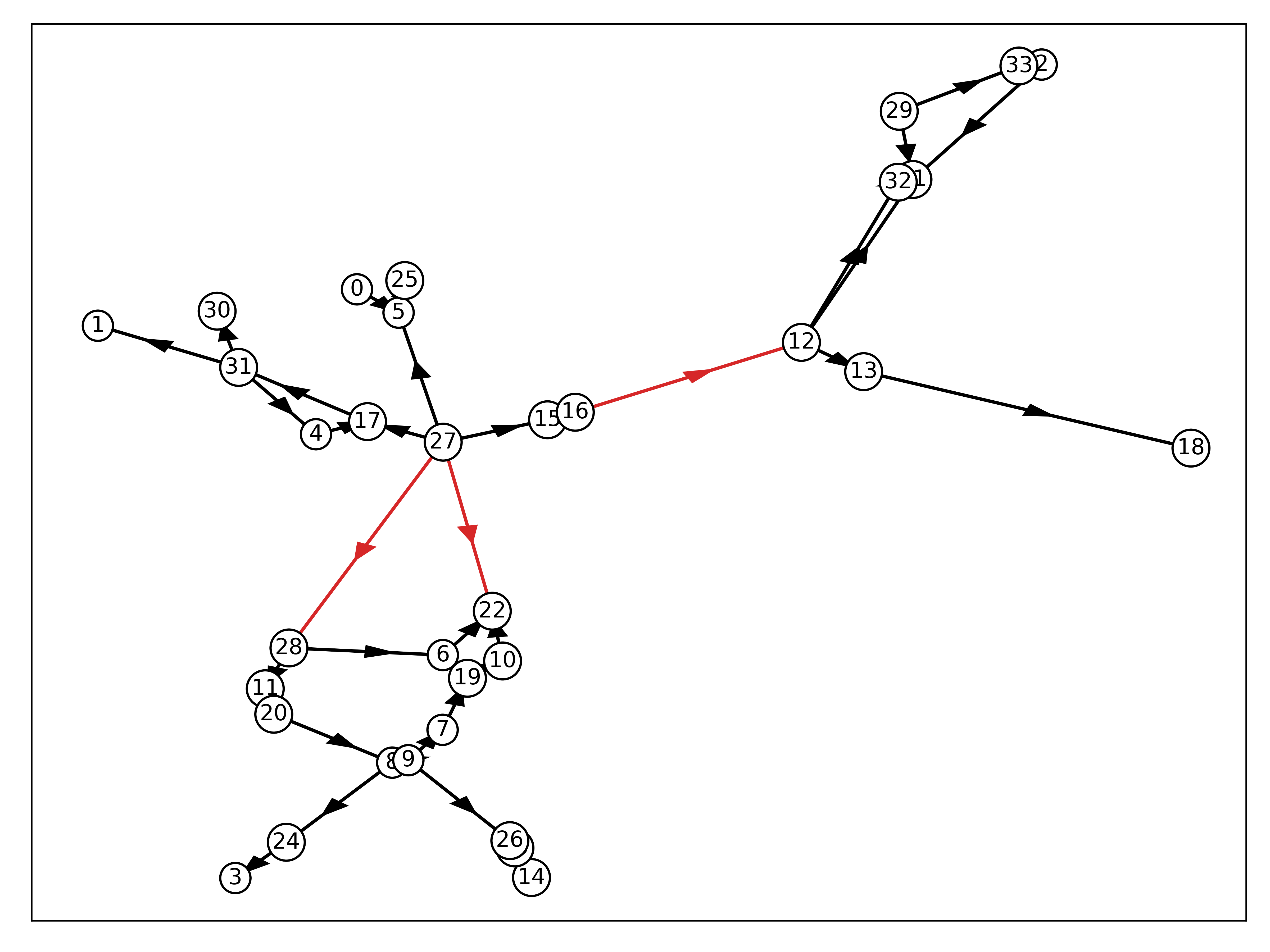
Figure 1: Sketch of the network for the numerical experiments. The arrows show the direction of the orientation of the pipes, which in general does not coincide with the direction of the flow. In red we have marked the edges on which the initial pressure for the original system and the observer system differ.

7.1 Discontinuous initial data and friction

The initial data for the first experiment is a piecewise constant function, i.e., the initial pressure on the pipes connecting nodes 12 and 16, 27 and 28, 22 and 27 (see Figure 1) is $$60\text{\,}\mathrm{b}\mathrm{a}\mathrm{r}$+h^{e}$ on the half of the pipes adjacent to the node with smaller index and $60\text{\,}\mathrm{b}\mathrm{a}\mathrm{r}$ on the other half of the pipe. For the system ($\mathbf{S}$) we have used $h^{e}=$2\text{\,}\mathrm{b}\mathrm{a}\mathrm{r}$$ for the edges connecting nodes 12 and 16, 27 and 28 and $h^{e}=$1\text{\,}\mathrm{b}\mathrm{a}\mathrm{r}$$ for the edge between node 22 and 27, while for the observer system ($\mathbf{R}$) we have used $h^{e}=$1.5\text{\,}\mathrm{b}\mathrm{a}\mathrm{r}$$ and $h^{e}=$0.75\text{\,}\mathrm{b}\mathrm{a}\mathrm{r}$$, respectively. For all other pipes, the initial pressure is constant $60\text{\,}\mathrm{b}\mathrm{a}\mathrm{r}$ for both systems.

We plot the result for $\mathcal{L}_{0}$ in Figure 2. As predicted, $\mathcal{L}_{0}$ decays exponentially for all cases except for $\mu^{v}=1$ at all nodes, which is in accordance with the theoretical results. As expected, we see the fastest convergence for $\mu^{v}=0$ at all nodes. In addition, snapshots of the difference of the numerical solutions at times $t=$0\text{\,}\mathrm{s}$$, $t\approx$90\text{\,}\mathrm{s}$$ and $t\approx$180\text{\,}\mathrm{s}$$ for $\mu^{v}=0$ at all nodes are shown in Figure 3. The pictures show that the difference $\delta$ between the two systems decreases over time.

Figure 2: Discontinuous initial data and friction: Temporal evolution of $\mathcal{L}_{0}$ for different values of $\mu^{v}$. In all but one cases we have set the same value of $\mu^{v}$ for all nodes, while ‘mixed’ means that $\mu^{v}=0$ at all nodes with even index and additionally at the nodes 1, 5, 7, 15, 17, 29 and $\mu^{v}=1$ for the remaining nodes.

Figure 3: Discontinuous initial data and friction: Snapshots of solutions at times $t=$0\text{\,}\mathrm{s}$$, $t\approx$90\text{\,}\mathrm{s}$$ and $t\approx$180\text{\,}\mathrm{s}$$ for $\mu^{v}=0$ at all nodes. On all pipes, $\delta_{+}$ is a red continuous line, $\delta_{-}$ is a blue dashed line and the network is shown by black dotted lines.

7.2 Discontinuous initial data without friction

For this experiment we use the same initial data as in the previous section but set the friction to zero (that is $\theta=0$). We plot the result for $\mathcal{L}_{0}$ in Figure 4. Again, $\mathcal{L}_{0}$ decays exponentially for $|\mu^{v}|<1$ at all nodes and for the ‘mixed’ case. It can be seen that, in the case $\mu^{v}=0$ at all nodes, $\mathcal{L}_{0}$ vanishes after about $257.5\text{\,}\mathrm{s}$, which is approximately the time that a wave needs to travel through the longest pipe (that connects nodes 27 and 28 and has a length of about $86.7\text{\,}\mathrm{k}\mathrm{m}$).

For the case $\mu^{v}=0$ on half of the nodes and $\mu^{v}=1$ at the remaining nodes, $\mathcal{L}_{0}$ vanishes after about $385\text{\,}\mathrm{s}$. So in the case of a source term that is zero, the observer and the original system can be synchronized in finite-time.

In addition, snapshots of the difference of the numerical solutions at times $t=$0\text{\,}\mathrm{s}$$, $t\approx$90\text{\,}\mathrm{s}$$ and $t\approx$180\text{\,}\mathrm{s}$$ for $\mu^{v}=0$ at all nodes are shown in Figure 5. The pictures show that the discontinuities in the solution remain, since the discretization of the convective terms produces no numerical diffusion.

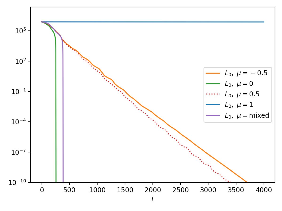
Figure 4: Discontinuous initial data without friction: Temporal evolution of $\mathcal{L}_{0}$ for different values of $\mu^{v}$. In all but one case we have set the same value of $\mu^{v}$ for all nodes, while ‘mixed’ means that $\mu^{v}=0$ at all nodes with even index and additionally at the nodes 1, 5, 7, 15, 17, 29 and $\mu^{v}=1$ for the remaining nodes.

Figure 5: Discontinuous initial data without friction: Snapshots of solutions at times $t=$0\text{\,}\mathrm{s}$$, $t\approx$90\text{\,}\mathrm{s}$$ and $t\approx$180\text{\,}\mathrm{s}$$ for $\mu^{v}=0$ at all nodes. On all pipes, $\delta_{+}$ is a red continuous line, $\delta_{-}$ is a blue dashed line and the network is shown by black dotted lines.

7.3 Continuous initial data and friction

In this experiment the initial pressure is a continuous function, i.e., the initial pressure on the pipes connecting nodes 12 and 16, 27 and 28, 22 and 27 (see Figure 1) is ${p(x)=\left(60+h^{e}\sin(f^{e}\frac{\pi x}{L})\right)\text{bar}}$. For the system ($\mathbf{S}$) we have used $h^{e}=2$ and $f^{e}=2$ for the edges connecting nodes 12 and 16, 27 and 28 and $h^{e}=1$, $f^{e}=4$ for the edge between node 22 and 27, while for the observer system ($\mathbf{R}$) we have used $h^{e}=1.5$, $f^{e}=2$ and $h^{e}=0.75$, $f^{e}=4$, respectively. For all other pipes, the initial pressure is constant $60\text{\,}\mathrm{b}\mathrm{a}\mathrm{r}$ for both systems.

We plot the results for $\mathcal{L}_{0}$ and $\mathcal{L}_{1}$ in Figure 6. As in the experiment with discontinuous initial data, $\mathcal{L}_{0}$ converges exponentially to zero for $|\mu^{v}|<1$ at all nodes and for the ’mixed’ case. Here we show additionally the value of $\mathcal{L}_{1}$, which also converges exponentially except in the case $\mu^{v}=1$ at all nodes.

The snapshots of the difference of the numerical solutions at times $t=$0\text{\,}\mathrm{s}$$, $t\approx$90\text{\,}\mathrm{s}$$ and $t\approx$180\text{\,}\mathrm{s}$$ for $\mu^{v}=0$ at all nodes, displayed in Figure 7, show that the difference already reduces significantly in the first $180\text{\,}\mathrm{s}$.

Figure 6: Continuous initial data and friction: Temporal evolution of $\mathcal{L}_{0}$ (left) and $\mathcal{L}_{1}$ (right) for different values of $\mu^{v}$. In all but one case we have set the same value of $\mu^{v}$ for all nodes, while ‘mixed’ means that $\mu^{v}=0$ at all nodes with even index and additionally at the nodes 1, 5, 7, 15, 17, 29 and $\mu^{v}=1$ for the remaining nodes.

Figure 7: Continuous initial data and friction: Snapshots of solutions at times $t=$0\text{\,}\mathrm{s}$$, $t\approx$90\text{\,}\mathrm{s}$$ and $t\approx$180\text{\,}\mathrm{s}$$ for $\mu^{v}=0$ at all nodes. On all pipes, $\delta_{+}$ is a red continuous line, $\delta_{-}$ is a blue dashed line and the network is shown by black dotted lines.

7.4 Continuous initial data without friction

Now we consider the case without friction, while we use the same initial data as in the previous experiment. We plot the results for $\mathcal{L}_{0}$ and $\mathcal{L}_{1}$ in Figure 8. Similar to the experiment for discontinuous initial data without friction, $\mathcal{L}_{0}$ and $\mathcal{L}_{1}$ vanish after about $257.5\text{\,}\mathrm{s}$ for $\mu^{v}=0$ at all nodes and after about $512.5\text{\,}\mathrm{s}$ for the ‘mixed’ case.

The snapshots of the difference of the numerical solutions at times $t=$0\text{\,}\mathrm{s}$$, $t\approx$90\text{\,}\mathrm{s}$$ and $t\approx$180\text{\,}\mathrm{s}$$ for $\mu^{v}=0$ at all nodes in Figure 9 show that the difference is zero on large parts of the network after $180\text{\,}\mathrm{s}$.

Figure 8: Continuous initial data without friction: Temporal evolution of $\mathcal{L}_{0}$ (left) and $\mathcal{L}_{1}$ (right) for different values of $\mu^{v}$. In all but one case we have set the same value of $\mu^{v}$ for all nodes, while ‘mixed’ means that $\mu^{v}=0$ at all nodes with even index and additionally at the nodes 1, 5, 7, 15, 17, 29 and $\mu^{v}=1$ for the remaining nodes.

Figure 9: Continuous initial data without friction: Snapshots of solutions at times $t=$0\text{\,}\mathrm{s}$$, $t\approx$90\text{\,}\mathrm{s}$$ and $t\approx$180\text{\,}\mathrm{s}$$ for $\mu^{v}=0$ at all nodes. On all pipes, $\delta_{+}$ is a red continuous line, $\delta_{-}$ is a blue dashed line and the network is shown by black dotted lines.

8 Conclusion

In this paper, we have analyzed the performance of an observer system for the gas flow through a pipeline network that is governed by a semilinear model. As input data for the observer system, measurement data that is obtained at certain points in space in the network is used. We have shown that under suitable regularity conditions for the solution the observation error decays exponentially. The theoretical findings are illustrated by numerical experiments.