]also at Jawaharlal Nehru Centre For Advanced Scientific Research, Jakkur, Bangalore, India

Arrhythmogenicity of cardiac fibrosis: fractal measures and Betti numbers

Abstract

Infarction- or ischaemia-induced cardiac fibrosis can be arrythmogenic. We use mathematcal models for diffuse fibrosis ($\mathcal{DF}$), interstitial fibrosis ($\mathcal{IF}$), patchy fibrosis ($\mathcal{PF}$), and compact fibrosis ($\mathcal{CF}$) to study patterns of fibrotic cardiac tissue that have been generated by new mathematical algorithms. We show that the fractal dimension $\mathbb{D}$, the lacunarity $\mathcal{L}$, and the Betti numbers $\beta_{0}$ and $\beta_{1}$ of such patterns are fibrotic-tissue markers that can be used to characterise the arrhythmogenicity of different types of cardiac fibrosis. We hypothesize, and then demonstrate by extensive in silico studies of detailed mathematical models for cardiac tissue, that the arrhytmogenicity of fibrotic tissue is high when $\beta_{0}$ is large and the lacunarity parameter $b$ is small.

Sudden cardiac death (SCD) continues to be a leading cause of death in the industrialised world (see, e.g., Refs. Kawara et al. (2001); Biernacka and Frangogiannis (2011); Nguyen et al. (2014); Hinderer and Schenke-Layland (2019) and  SCA Foundation ). Even young athletes Stormholt et al. (2021) may be victims of SCD; and a recent study has suggested that there is a correlation between out-of-hospital cardiac arrest and COVID-19  Baldi et al. (2020); Kuck (2020). Ventricular arrhythmias, such as ventricular tachycardia (VT) and ventricular fibrillation (VF), are often the root cause of SCDs Mehra (2007); Rubart et al. (2005). Myocardial infarction and ischaemia lead to cardiac-tissue fibrosis, which is one of the important contributors to arrhythmogenesis, and, therefore, to SCDs. Several experimental studies, such as those in Refs. Kawara et al. (2001); Hocini et al. (2002); Balaban et al. (2018), have demonstrated the arrythmogenicity of cardiac fibrosis, which induces reentry by delaying local conduction. Fibrosis has been observed to alter the dynamics of the electrical waves passing through fibrotic regions; this leads to the formation of re-entrant waves that can precipitate cardiac arrythmias Majumder et al. (2012); Morgan et al. (2016); Jousset et al. (2016); Clayton (2018).

In the heart, fibrotic tissue is made up of cardiac fibroblast cells or collagen fibers; and it has been classified visually Nguyen et al. (2014); Hansen et al. (2017) into four different types with (a) diffuse fibrosis ($\mathcal{DF}$), (b) interstitial fibrosis ($\mathcal{IF}$), (c) patchy fibrosis ($\mathcal{PF}$), and (d) compact fibrosis ($\mathcal{CF}$). However, in-vivo, ex-vivo, or in-vitro studies have not been used hitherto for a quantitative statistical characterization of these types of fibrosis, perhaps because large-enough data sets of images are not available. We show, via detailed analysis, that recently developed mathematical models Jakes et al. (2019) for fibrotic tissue, which use Perlin noise, and idealised models, which we define below, can be used to distinguish quantitatively between $\mathcal{DF}$, $\mathcal{IF}$, $\mathcal{CF}$, and $\mathcal{PF}$ by obtaining the fractal dimension $\mathbb{D}$, the lacunarity $\mathcal{L}(\epsilon)$, and Betti numbers $\beta_{0}$ and $\beta_{1}$ (see, e.g., Refs. de la Calleja and Zenit (2020); Gould et al. (2011)) of patterns of fibrotic tissue. For fibrosis patterns, which we obtain from Perlin noise, we employ the notations $\mathcal{DFP}$, $\mathcal{IFP}$, $\mathcal{CFP}$, and $\mathcal{PFP}$ for diffuse, interstitial, patchy, and compact fibrosis, respectively; their counterparts for the idealised model are $\mathcal{DFI}$, $\mathcal{IFI}$, $\mathcal{CFI}$, and $\mathcal{PFI}$. We show how to compute such properties by the digitisation of images of fibrotic tissue. These properties serve as fibrotic-tissue markers; and they can be used to characterise the arrhythmogenicity of different types of cardiac fibrosis. We hypothesize, and then demonstrate by extensive in silico studies of detailed mathematical models for cardiac tissue, that the arrhythmogenicity of fibrotic tissue is high when $\beta_{0}$ is large and the lacunarity parameter $b$ is small. Our study has implications for clinical cardiology, because, even at a qualitative level, we find that (a) $\mathcal{DF}$ is most arrythogenic and (b) $\mathcal{CF}$ is least arrythmogenic.

For the dynamics of cardiac myocytes we use the biologically realistic human-ventricular-cell model Ten Tusscher and Panfilov (2006), due to ten Tusscher and Panfilov (henceforth, the TP06 model), in which the spatiotemporal evolution of the transmembrane potential $V_{m}$ is governed by the following reaction-diffusion partial differential equation (PDE):

$$\frac{\partial{{V_{m}}}}{\partial{t}}+\frac{I_{{ion}}}{C_{m}}=\nabla.(D\nabla{V_{m}});$$ (1)

here, $I_{ion}$ is the sum of all the ionic currents (Eq. 2), $C_{m}$ is the membrane capacitance, and, in the case of tissue with healthy myocytes, we use a scalar diffusion constant $D=0.00154\ cm^{2}/ms$; in the region of the tissue with fibrosis and with collageneous fibers we use $D=0$.

$$I_{ion} = I_{Na}+I_{CaL}+I_{to}+I_{Ks}+I_{Kr}+I_{K1}+I_{NaCa}$$ (2)

$$+ I_{NaK}+I_{pCa}+I_{pK}+I_{bNa}+I_{bCa}.$$

For the details of the currents we refer the reader to the Ref. Ten Tusscher and Panfilov (2006); and we use the standard TP06-model parameters Ten Tusscher and Panfilov (2006) for ion-channel conductances. We obtain the ordinary differential equation (ODE) for a single cardiomyocyte by setting $D=0$ in Eq. 1. Our model for cardiac tissue has three types of regions:

• those in which we have normal, TP06-model mycoytes that evolve according to Eq. 1 with $D=0.00154\ cm^{2}/ms$;

• in the vicinities of fibrotic areas, there are regions in which remodelled cardiomyocytes evolve according to Eq. 1, with $D=0.00154\ cm^{2}/ms$, but with modified conductances [we change the maximal ion-channel conductances $G_{Na},\ G_{CaL},\ G_{Kr}\ \text{and}\ G_{Ks}$, in the TP06 model, to $0.38*G_{Na},\ 0.31*G_{CaL},\ 0.3*G_{Kr}\ \text{and}\ 0.2*G_{Ks}$, respectively, (see, e.g., Ref. Zlochiver et al. (2008); McDowell et al. (2011); Nguyen et al. (2014))];

• fibrotic-tissue regions in which we set $D=0$.

First we show the effect of remodeling on a single myocyte cell. In Fig. 1 we contrast the action potential (AP) of a normal-myocyte (NM) and a remodelled-myocyte (RM): The upstroke-velocity $\frac{dV}{dt}_{max}$ of the AP decreases and the action-potential duration (APD) increases if we replace a NM by RM. Furthermore, when we pace these myocytes, with a pacing frequency of $2.5$ Hz, we observe alternans only in RM. We expect, therefore, that in those parts of the tissue that have RMs the conduction velocity of the wave decreases and its wavelength $\lambda$ increases. (For the importance of such remodeling, see Fig. S5 in the Supplemental Material Sup .)

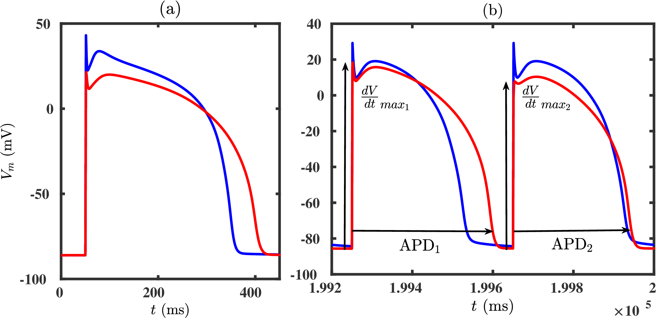
Figure 1: (Color online) Plots from our simulations of APs of normal (NM) [blue] and remodelled (RM) [red] myocytes: (A) Both the NM and the RM are given a single stimulus pulse; and (B) the $1000^{th}$ and $999^{th}$ APs of NM and RM that are paced with a pacing frequency of PCL=$400$ ms ($2.5$ Hz); here, we observe alternans for the RM but not for the NM.

We use the following two classes of mathematical models for the organization of fibrotic tissue:

• (A) A recently developed model Jakes et al. (2019) yields fibrotic textures of types $\mathcal{DF}$, $\mathcal{IF}$, $\mathcal{PF}$, and $\mathcal{CF}$, for which we give illustrative plots in Figs. 2 (a), (b), (c), and (d), respectively, with normal (yellow) and fibrotic (blue) regions. This model creates synthetic textures, for different types of fibrotic tissue, by using Perlin noise and approximate Bayesian computation Jakes et al. (2019); these textures match well with those observed in experiments.

• (B) Idealised models, which we define below, in a square region ($R\times R$ grid of myocytes); these models include parameters like $p_{f}$, the percentage of fibrotic sites, and $\theta\ \in\ [0,\pi]$, the angle that fibrotic strands make with the horizontal axis; these parameters can be tuned easily.

  • (i) $\mathcal{DFI}$: we replace, randomly, a percentage $p_{f}$ of myocytes by fibrotic, nonconducting ($D=0$) sites (Fig. 2 (e));

  • (ii) $\mathcal{IFI}$: we introduce long, thin strands of non-conducting fibers ($D=0$), with orientation $\theta$; fiber thickness: $2-3$ grid points; fiber lengths go from a minimum of $2$ to at most $50-60$ grid points (Fig. 2 (f)).

  • (iii) $\mathcal{PFI}$: we use strands, as in $\mathcal{IF}$, but with two different angles for interstitial fibers, say $\theta_{1}=60^{\circ}$ and $\theta_{2}=90^{\circ}+60^{\circ}$, with thicknesses and lengths of $2-3$ grid points; at the intersection of fibers, we add small patches of diffuse fibrosis with $p_{f}=5-10\%$ (Fig. 2 (g)).

  • (iv) $\mathcal{CFI}$: we generate compact regions with random shapes (Fig. 2 (h)) by using the pinta software (Ref. Pinta ), a program for drawing.

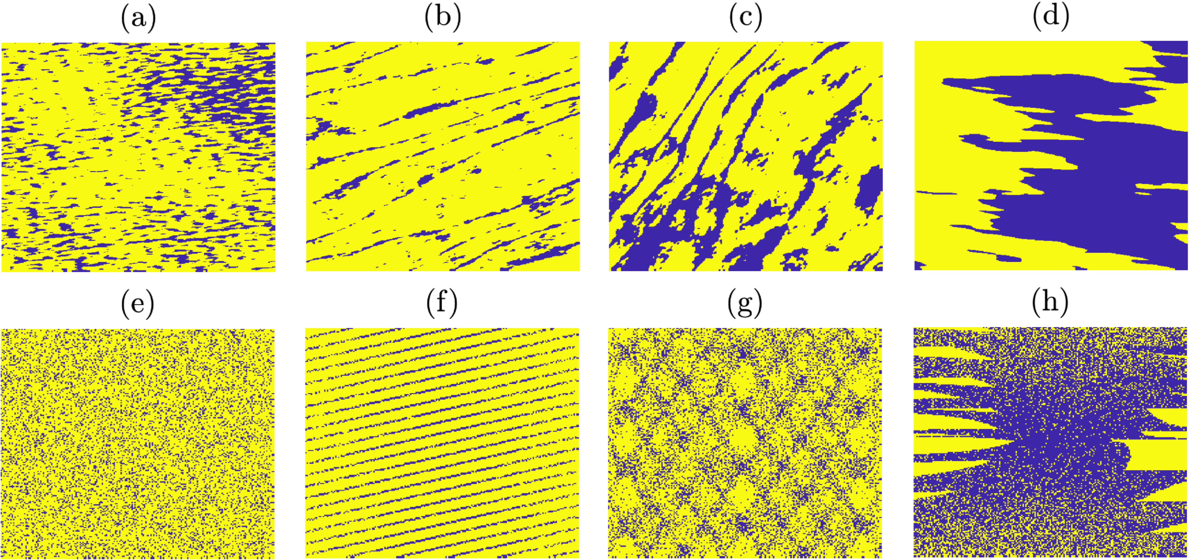
Figure 2: (Color online) Illustrative plots of fibrotic textures of types (a) $\mathcal{DFP}$, (b) $\mathcal{IFP}$, (c) $\mathcal{PFP}$, and (d) $\mathcal{CFP}$, from the Perlin-noise model (A) (see text and Ref.  Jakes et al. (2019)); regions with myocytes and with fibrotic tissue are indicated in yellow and blue, respectively. (e) $\mathcal{DFI}$, (f) $\mathcal{IFI}$, (g) $\mathcal{PFI}$, and (g) $\mathcal{CFI}$ in the second row are the counterparts of (a)-(d) for the idealised model (B) (see text).

Arrhythmogenicity arises because of the interaction between the wave of electrical activation and the fibrotic tissue. The ratio of the wavelength of this wave and the linear size of the fibrotic tissue is an important control parameter Ref. Majumder et al. (2014); Zimik and Pandit (2017). We use the following simulation domains: (a) For the Perlin-noise model (A): a square domain with $720\times 720$ grid points; most of the sites in these domains contain normal myocytes, except in a central fibrotic region with $400\times 250$ grid points. (b) For the idealised model (B): a square domain with $512\times 512$ grid points, with normal myocytes, except in a central fibrotic region with $200\times 200$ grid points. The area fractions of fibrotic regions are $\simeq 0.19$ and $\simeq 0.15$ in domains (a) and (b), respectively. In our numerical simulations, we use fixed time and space steps $\Delta t=0.02\ ms$ and $\Delta x=0.025\ cm$, respectively, and a finite-difference scheme, with a five-point stencil for the Laplacian in Eq. 1. The value of $D=0.00154\ cm^{2}/ms$ that we use leads to the experimentally observed conduction velocity $CV\simeq 70\ cm/s$ in a region with normal myocytes Ten Tusscher and Panfilov (2006).
A wave of electrical activation slows down in a region with RMs; this can lead to conduction blocks that are arrhythmogenic. We pace our simulation domain at its lower boundary with a high-frequency ($\omega=3.3$ Hz) current pulse. The resulting spatiotemporal evolution of $V_{m}$, given in the video V1 of the Supplemental Material Sup , shows the birth of proto spirals, a clear signature of arrhythmogenesis; we give illustrative pseudocolor plots of $V_{m}$ in Fig. 3 for $\mathcal{DF}$, $\mathcal{IF}$), $\mathcal{PF}$, and $\mathcal{CF}$ in models (A) [top row] and (B) [bottom row].

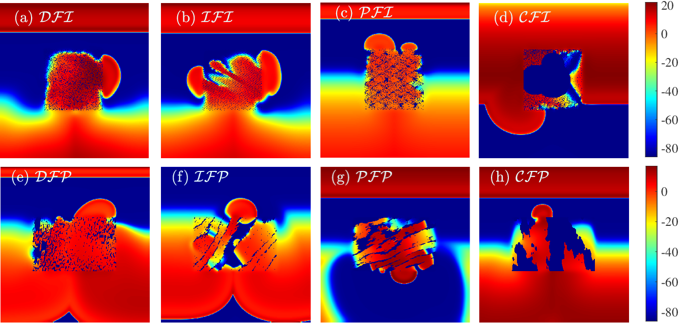
Figure 3: (Color online) Illustrative pseudocolor plots of $V_{m}$ when we pace our simulation domain at its lower boundary with a high-frequency ($\omega=3.3$ Hz) current pulse. (For the full spatiotemporal evolution of $V_{m}$ see the video V1 in the Supplemental Material Sup .) Top row for the idealised model (B): (a) $\mathcal{DFI}$; (b) $\mathcal{IFI}$; (c) $\mathcal{PFI}$; and (d) $\mathcal{CFI}$. Bottom row for the Perlin-noise model (A): (e) $\mathcal{DFP}$; (f) $\mathcal{IFP}$; (g) $\mathcal{PFP}$; and (h) $\mathcal{CFP}$.

To quantify the statistical properties of these fibrotic-tissue patterns, we first calculate their fractal dimensions $\mathbb{D}$ and lacunarity $\mathcal{L}(\epsilon)$ (see, e.g., Refs. de la Calleja and Zenit (2020); Gould et al. (2011)), at a length scale $\epsilon$, by using, respectively, the box-counting and gliding-box-counting algorithms Tolle et al. (2008); Gould et al. (2011). $\mathcal{L}(\epsilon)$, which measures the distribution of the sizes of lacunae, the degree of inhomogeneity, and translational and rotational invariance of a pattern Gould et al. (2011); Karperien and Jelinek (2015), is given by

$$\mathcal{L}(\epsilon)=\frac{N(\epsilon)Q_{1}}{Q_{2}},$$ (3)

where $N(\epsilon)$ is the number of square boxes of side $\epsilon$, $p(i,\epsilon)$ the number of signal pixels in the $i^{th}$ box with $i\in[1,N(\epsilon)]$, $Q_{1}\equiv\sum_{i}p(i,\epsilon)$, and $Q_{2}\equiv\sum_{i}p(i,\epsilon)^{2}$. For the values of $\epsilon$ we use, we find, as in Ref. Gould et al. (2011), that our data can be fit to the form

$$\mathcal{L}(\epsilon)=b\ \epsilon^{-a},$$ (4)

where $b$ is the lacunarity parameter and $a$ is the lacunarity exponent (see Figs. S4 and S5 in the Supplemental Material Sup ); a small value of $b$ leads to wide concavity in the hyperbolic fit (see Eq. 4). We also characterize these 2D fibrotic textures by their Betti numbers de la Calleja and Zenit (2020) $\beta_{0}$ and $\beta_{1}$, which measure, respectively, the number of connected components and the number of holes that are completely enclosed by occupied pixels (see Fig.S1 in the Supplemental Material Sup ). To obtain $\beta_{0}$ and $\beta_{1}$, we convert the fibrotic-tissue data sets into the bit-map (bmp) image format; and then we use the computational-homology-project software CHomP to get $\beta_{0}$ and $\beta_{1}$ for the particular fibrotic image.

In Fig. 4, we present plots of the mean number $\langle N_{r}\rangle$ of re-entries that we observe, while pacing the fibrotic tissue with PCL=$300$ ms in the idealised model (B); these data are averaged over $10$ realisations. The larger the value of $\langle N_{r}\rangle$, the more arrhythmogenic this tissue. In Fig. 4 (a) we plot $\langle N_{r}\rangle$ versus $p_{f}$ for $\mathcal{DFI}$; for $p_{f}>35\%$, there is no re-entry because of the very low conduction velocity of the excitations within the fibrotic region; but $\langle N_{r}\rangle>0$, for $0\%<p_{f}\leq 30\%$, so $\mathcal{DFI}$ is clearly arrhythmogenic. In Fig. 4 (b) we show how $\langle N_{r}\rangle$, for $\mathcal{IFI}$, depends on the angle $\theta$ of the inclination of the fibrotic strands with the pacing plane wave; $\langle N_{r}\rangle$ is highest in the range $\theta\simeq 75^{\circ}-105^{\circ}$ and it decreases outside this range. Clearly, $\theta$ is an important parameter which determines the arrhytmogenicity of $\mathcal{IFI}$. We find that $\langle N_{r}\rangle$ in $\mathcal{PFI}$ is comparable to that in $\mathcal{IFI}$. By contrast, $\mathcal{CFI}$ shows much lower values of $\langle N_{r}\rangle$ than the other types of fibrotic patterns.

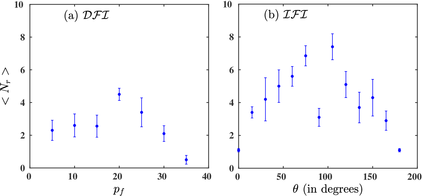
Figure 4: (Color online) Plots of the mean number $\langle N_{r}\rangle$ of re-entries that we observe, while pacing the fibrotic tissue with PCL=$300$ ms in the idealised model (B): (a) versus the percentage $p_{f}$ of randomly placed fibrotic sites (in $\mathcal{DFI}$); (b) versus the angle $\theta$ of the inclination of the fibrotic strands with the pacing plane wave (in $\mathcal{IFI}$).

In Fig. 5 we present, for the Perlin-noise model (A), plots versus the realisation number $r=1,2,\ldots,955$ of the fractal dimension $\mathbb{D}$ (left panel) and the lacunarity parameter (right panel) $b$, defined in Eq. 4, for all types of fibrotic regions, namely, $\mathcal{DFP}$ (blue), $\mathcal{IFP}$ (red), $\mathcal{PFP}$ (black), and $\mathcal{CFP}$ (pink); we use angular brackets for mean values. We see from these plots that $\mathbb{D}$ is the same (within error bars) for $\mathcal{DFP}$ and $\mathcal{PFP}$; however, these four different fibrotic patterns are distinguished clearly by their lacunarity parameters $b$.

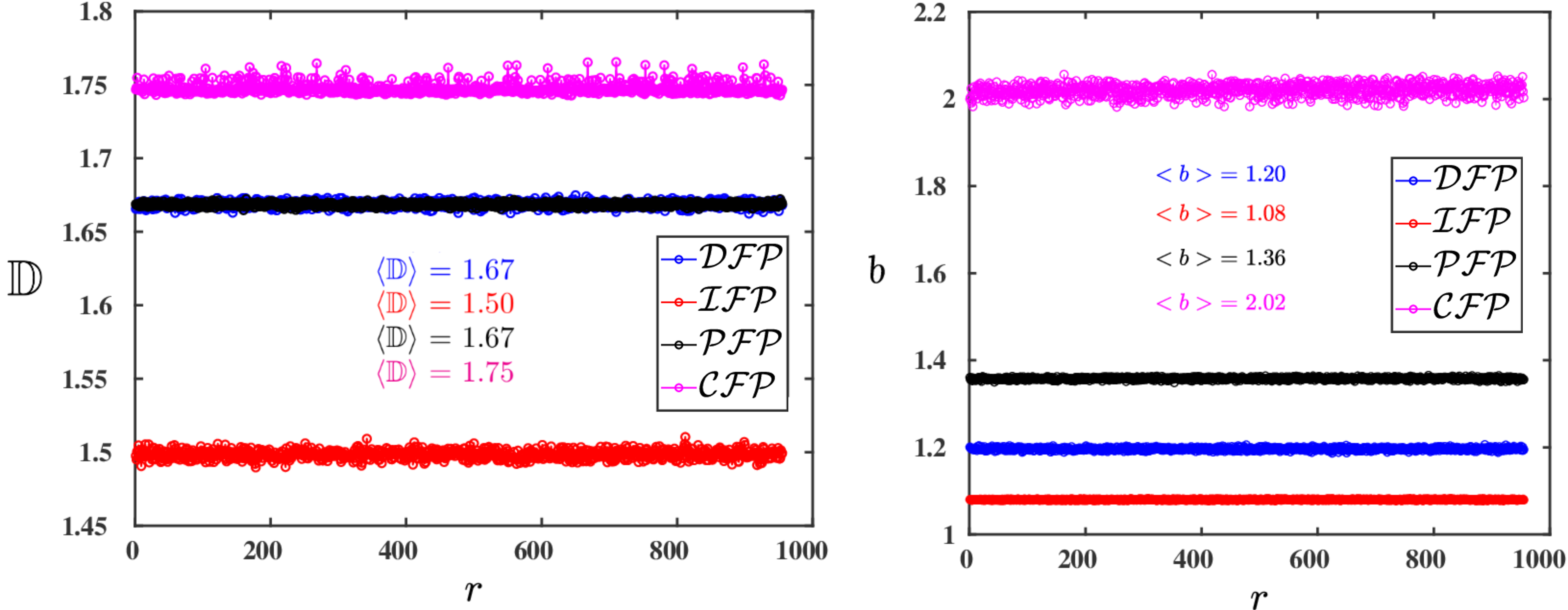
Figure 5: (Color online) Plots versus the realisation number $r=1,2,\ldots,955$, for the Perlin-noise model (A), of the fractal dimension $\mathbb{D}$ (left panel) and the lacunarity parameter $b$ (right panel) in Eq. 4 fibrotic regions of types $\mathcal{DFP}$ (blue), $\mathcal{IFP}$ (red), $\mathcal{PFP}$ (black), and $\mathcal{CFP}$ (pink); we use angular brackets for mean values.

In Fig. 6 we present, in the top row, plots versus the realisation number $r=1,2,\ldots,955$, for the Perlin-noise model (A), of the Betti numbers $\beta_{0}$ (blue) and $\beta_{1}$ (red) for (a) $\mathcal{DFP}$, (b) $\mathcal{IFP}$, (c) $\mathcal{PFP}$, and (d) $\mathcal{CFP}$; we use angular brackets for mean values. In the bottom row of Fig. 6 we give histograms of $N_{r}$, which we obtain from $150$ model-(A) realizations of the fibrotic regions $\mathcal{DFP}$, $\mathcal{IFP}$, $\mathcal{PFP}$, and $\mathcal{CFP}$; here, $\mu$ and $\sigma$ denote, respectively, the mean and standard deviation.

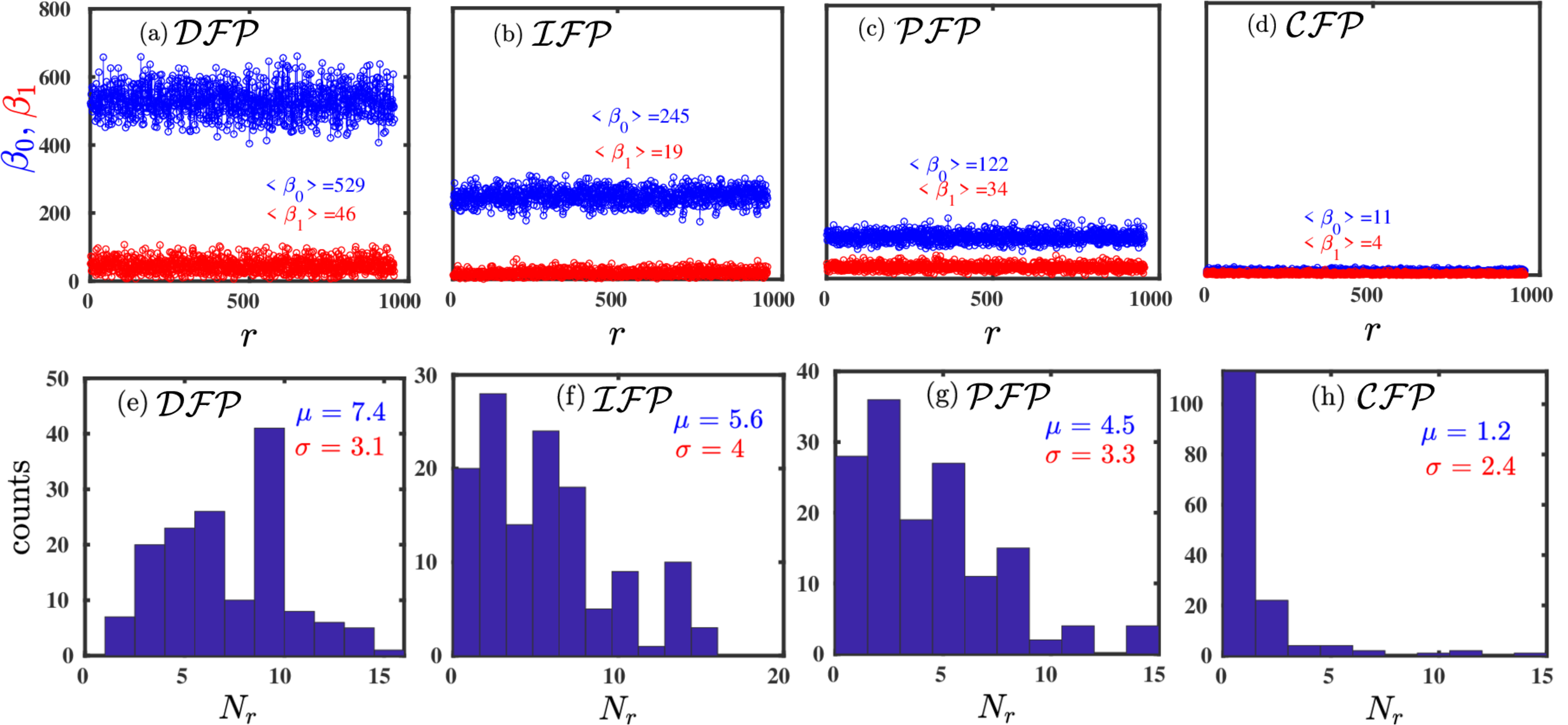
Figure 6: (Color online) Plots versus the realisation number $r=1,2,\ldots,955$, for the Perlin-noise model (A), of the Betti numbers $\beta_{0}$ (blue) and $\beta_{1}$ (red) for (a) $\mathcal{DFP}$, (b) $\mathcal{IFP}$, (c) $\mathcal{PFP}$, and (d) $\mathcal{CFP}$; we use angular brackets for mean values. Histograms of $N_{r}$, for $150$ model-(B) realizations of fibrotic regions, for (e) $\mathcal{DFP}$, (f) $\mathcal{IFP}$, (g) $\mathcal{PFP}$, and (h) $\mathcal{CFP}$; $\mu$ and $\sigma$ are, respectively, the mean and standard deviation.

We conclude from Figs. 5 and 6 that fibrotic patterns with small values of $b$ and with large values of $\beta_{0}$ are most arrhythmogenic. We show this explicitly for model-(B) realizations of $\mathcal{DFI}$ in Fig. 7: In Fig. 7(a), we plot versus $p_{f}$ the Betti numbers $\beta_{0}$ (blue) and $\beta_{1}$ (maroon), and the lacunarity parameter $b$ (green); the light-green rectangle indicates the region in which there is significant re-entry with a significant value of $\langle N_{r}\rangle$. In Fig. 7(b) we plot, versus $p_{f}$, $N_{r}/\langle N_{r}\rangle$ (blue curve) and $n_{r}/\langle n_{r}\rangle$ (pink curve), where $n_{r}\equiv\beta_{0}/b$; these curves (blue and pink) are correlated to the extent that they are large in the same range of values of $p_{f}$.

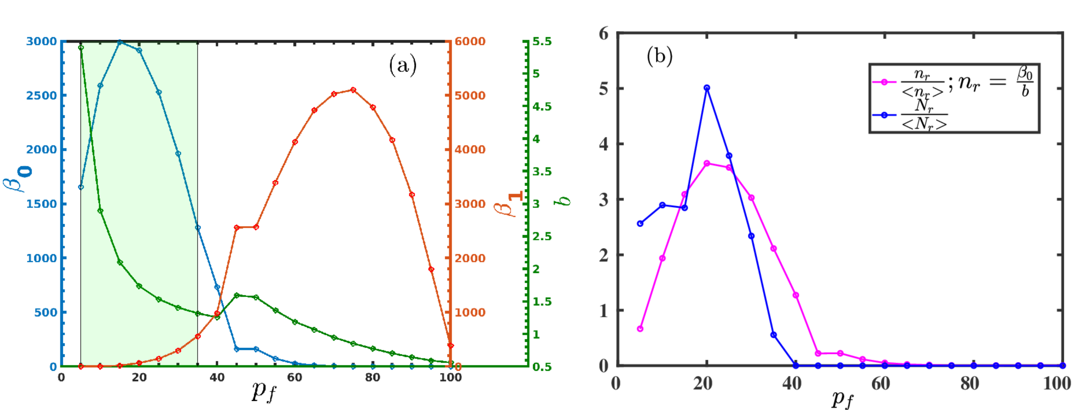
Figure 7: (Color online) Plots versus $p_{f}$: (a) the Betti numbers $\beta_{0}$ (blue) and $\beta_{1}$ (maroon) and the lacunarity parameter $b$ (green); the light-green rectangle indicates the region in which $\langle N_{r}\rangle$ is significant; (b) $N_{r}/\langle N_{r}\rangle$ (blue curve) and $n_{r}/\langle n_{r}\rangle$ (pink curve).

Earlier computational studies of cardiac-tissue fibrosis include Refs. Zlochiver et al. (2008); Xie et al. (2009); McDowell et al. (2011); Nayak et al. (2013); Nayak and Pandit (2015); Ten Tusscher and Panfilov (2007); Majumder et al. (2012); Alonso et al. (2016); these are, roughly speaking, of two different types: (A) those that model the myocyte-fibroblast coupling Zlochiver et al. (2008); Xie et al. (2009); McDowell et al. (2011); Nayak et al. (2013); Nayak and Pandit (2015); and (b) those that use geometrical modeling for $\mathcal{DF}$ tissue Ten Tusscher and Panfilov (2007); Majumder et al. (2012); Alonso et al. (2016). There have been no studies, heretofore, which have investigated arrhythmogenesis, systematically and simultaneously, in all four types of fibrotic tissue. Our study leads to a natural way of quantifying the arrhythmogenicity of diffuse fibrosis ($\mathcal{DF}$), interstitial fibrosis ($\mathcal{IF}$), patchy fibrosis ($\mathcal{PF}$), and compact fibrosis ($\mathcal{CF}$) in cardiac tissue. We have shown that the statistical properties of these fibrotic-tissue patterns, such as their fractal dimension $\mathbb{D}$, lacunarity parameter $b$, and Betti numbers $\beta_{0}$ and $\beta_{1}$ are important in determining the arrhythmogenicity of fibrotic tissue. Our work sets the stage for (a) to experimental investigations of arrhythmogenesis in $\mathcal{DF}$, $\mathcal{IF}$, $\mathcal{PF}$, and $\mathcal{CF}$ and (b) in silico studies of such studies that go beyond our model by using anatomically realistic simulation domains, with muscle-fiber orientation, realistic myocyte-fibroblast couplings, and bidomain models.