Data Augmentation in High Dimensional Low Sample Size Setting Using a Geometry-Based Variational Autoencoder

Abstract

In this paper, we propose a new method to perform data augmentation in a reliable way in the High Dimensional Low Sample Size (HDLSS) setting using a geometry-based variational autoencoder (VAE). Our approach combines the proposal of 1) a new VAE model, the latent space of which is modeled as a Riemannian manifold and which combines both Riemannian metric learning and normalizing flows and 2) a new generation scheme which produces more meaningful samples especially in the context of small data sets. The method is tested through a wide experimental study where its robustness to data sets, classifiers and training samples size is stressed. It is also validated on a medical imaging classification task on the challenging ADNI database where a small number of 3D brain magnetic resonance images (MRIs) are considered and augmented using the proposed VAE framework. In each case, the proposed method allows for a significant and reliable gain in the classification metrics. For instance, balanced accuracy jumps from 66.3% to 74.3% for a state-of-the-art convolutional neural network classifier trained with 50 MRIs of cognitively normal (CN) and 50 Alzheimer disease (AD) patients and from 77.7% to 86.3% when trained with 243 CN and 210 AD while improving greatly sensitivity and specificity metrics.

1 Introduction

Even though always larger data sets are now available, the lack of labeled data remains a tremendous issue in many fields of application. Among others, a good example is healthcare where practitioners have to deal most of the time with (very) low sample sizes (think of small patient cohorts) along with very high dimensional data (think of neuroimaging data that are 3D volumes with millions of voxels). Unfortunately, this leads to a very poor representation of a given population and makes classical statistical analyses unreliable [1, 2]. Meanwhile, the remarkable performance of algorithms heavily relying on the deep learning framework [3] has made them extremely attractive and very popular. However, such results are strongly conditioned by the number of training samples since such models usually need to be trained on huge data sets to prevent over-fitting or to give statistically meaningful results [4].

A way to address such issues is to perform data augmentation (DA) [5]. In a nutshell, DA is the art of increasing the size of a given data set by creating synthetic labeled data. For instance, the easiest way to do this on images is to apply simple transformations such as the addition of Gaussian noise, cropping or padding, and assign the label of the initial image to the created ones. While such augmentation techniques have revealed very useful, they remain strongly data dependent and limited. Some transformations may indeed be uninformative or even induce bias. For instance, think of a digit representing a 6 which gives a 9 when rotated. While assessing the relevance of augmented data may be quite straightforward for simple data sets, it reveals very challenging for complex data and may require the intervention of an expert assessing the degree of relevance of the proposed transformations. In addition to the lack of data, imbalanced data sets also severely limit generalizability since they tend to bias the algorithm toward the most represented classes. Oversampling is a method that aims at balancing the number of samples per class by up-sampling the minority classes. The Synthetic Minority Over-sampling TEchnique (SMOTE) was first introduced in [6] and consists in interpolating data points belonging to the minority classes in their feature space. This approach was further extended in other works where the authors proposed to over-sample close to the decision boundary using either the $k$-Nearest Neighbor ($k$-NN) algorithm [7] or a support vector machine (SVM) [8] and so insist on samples that are potentially misclassified. Other over-sampling methods aiming at increasing the number of samples from the minority classes and taking into account their difficulty to be learned were also proposed [9, 10]. However, these methods hardly scale to high-dimensional data [11, 12].

The recent rise in performance of generative models such as generative adversarial networks (GAN) [13] or variational autoencoders (VAE) [14, 15] has made them very attractive models to perform DA. GANs have already seen a wide use in many fields of application [16, 17, 18, 19, 20], including medicine [21]. For instance, GANs were used on magnetic resonance images (MRIs) [22, 23], computed tomography (CT) [24, 25], X-ray [26, 27, 28], positron emission tomography (PET) [29], mass spectroscopy data [30], dermoscopy [31] or mammography [32, 33] and demonstrated promising results. Nonetheless, most of these studies involved either a quite large training set (above 1000 training samples) or quite small dimensional data, whereas in everyday medical applications it remains very challenging to gather such large cohorts of labeled patients. As a consequence, as of today, the case of high dimensional data combined with a very low sample size remains poorly explored. When compared to GANs, VAEs have only seen a very marginal interest to perform DA and were mostly used for speech applications [34, 35, 36]. Some attempts to use such generative models on medical data either for classification [37, 38] or segmentation tasks [39, 40, 41] can nonetheless be noted. The main limitation to a wider use of these models is that they most of the time produce blurry and fuzzy samples. This undesirable effect is even more emphasized when they are trained with a small number of samples which makes them very hard to use in practice to perform DA in the high dimensional (very) low sample size (HDLSS) setting.

In this paper, we argue that VAEs can actually be used for data augmentation in a reliable way even in the context of HDLSS data, provided that we bring some modeling of the latent space and amend the way we generate the data. Hence, in this paper we propose the following contributions:

• We propose a new geometry-aware VAE model, the latent space of which is seen as a Riemannian manifold and combining Riemannian metric learning and normalizing flows.

• We introduce a new non-prior based generation procedure consisting in sampling from the inverse of the Riemannian metric volume element learned by the model. The choice of this framework is discussed, motivated and compared to other VAE models.

• We propose to use such a framework to perform data augmentation in the challenging context of HDLSS data. The robustness of the augmentation method to data sets and classifiers changes along with its reliance to the number of training samples and the complexity of the classifier is then tested through a series of experiments.

• We validate the proposed method on several real-life classification tasks on complex 3D MRI from ADNI and AIBL databases where the augmentation method allows for a significant gain in classification metrics even when only 50 samples per class are considered.

2 Variational Autoencoder

In this section, we quickly recall the idea behind VAEs along with some proposed improvements relevant to this paper.

2.1 Model Setting

Let $x\in\mathcal{X}$ be a set of data. A VAE aims at maximizing the likelihood of a given parametric model $\{\mathbb{P}_{\theta},\theta\in\Theta\}$. It is assumed that there exist latent variables $z$ living in a lower dimensional space $\mathcal{Z}$, referred to as the latent space, such that the marginal distribution of the data can be written as:

$$p_{\theta}(x)=\int\limits_{\mathcal{Z}}p_{\theta}(x|z)q(z)dz\,,$$ (1)

where $q$ is a prior distribution over the latent variables acting as a regulation factor and $p_{\theta}(x|z)$ is most of the time taken as a simple parametrized distribution (e.g. Gaussian, Bernoulli, etc.). Such a distribution is referred to as the decoder, the parameters of which are usually given by neural networks. Since the integral of Eq. (1) is most of the time intractable, so is the posterior distribution:

$$p_{\theta}(z|x)=\frac{p_{\theta}(x|z)q(z)}{\int\limits_{\mathcal{Z}}p_{\theta}(x|z)q(z)dz}\,.$$

This makes direct application of Bayesian inference impossible and so recourse to approximation techniques such as variational inference [42] is needed. Hence, a variational distribution $q_{\phi}(z|x)$ is introduced and aims at approximating the true posterior distribution $p_{\theta}(z|x)$ [14]. This variational distribution is often referred to as the encoder. In the initial version of the VAE, $q_{\phi}$ is taken as a multivariate Gaussian whose parameters $\mu_{\phi}$ and $\Sigma_{\phi}$ are again given by neural networks. Importance sampling is then applied to get an unbiased estimate of $p_{\theta}(x)$ we want to maximize in Eq. (1)

$$\hat{p}_{\theta}(x)=\frac{p_{\theta}(x|z)q(z)}{q_{\phi}(z|x)}\hskip 5.69054pt\text{and}\hskip 5.69054pt\mathbb{E}_{z\sim q_{\phi}}\big{[}\hat{p}_{\theta}\big{]}=p_{\theta}(x)\,.$$ (2)

Using Jensen’s inequality allows finding a lower bound on the objective function of Eq. (1)

$$\log p_{\theta}(x) =\log\mathbb{E}_{z\sim q_{\phi}}\big{[}\hat{p}_{\theta}\big{]}$$ (3)

$$\geq\mathbb{E}_{z\sim q_{\phi}}\big{[}\log\hat{p}_{\theta}\big{]}$$

$$\geq\mathbb{E}_{z\sim q_{\phi}}\big{[}\log p_{\theta}(x|z)\big{]}-D_{KL}(q_{\phi}(z|x)\lVert p(z))\,.$$

The Evidence Lower BOund (ELBO) is now tractable since all distributions are known and so can be optimized with respect to the encoder and decoder parameters.

2.2 Improving the Model: Literature Review

In recent years, many attempts to improve the VAE model have been made and we briefly discuss three main areas of improvement that are relevant to this paper in this section.

2.2.1 Enhancing the Variational Approximate Distribution

When looking at Eq. (3), it can be noticed that we are nonetheless trying to optimize only a lower bound on the true objective function. Therefore, much efforts have been focused on making this lower bound tighter and tighter [43, 44, 45, 46, 47, 48]. One way to do this is to enhance the expressiveness of the approximate posterior distribution $q_{\phi}$. This is indeed due to the ELBO expression which can be also written as follows:

$$ELBO=\log p_{\theta}(x)-D_{KL}(q_{\phi}(z|x)||p_{\theta}(z|x))\,.$$

This expression makes two terms appear. The first one is the function we want to maximize while the second one is the Kullback–Leibler (KL) divergence between the approximate posterior distribution $q_{\phi}(z|x)$ and the true posterior $p_{\theta}(z|x)$. This very term is always non-negative and equals 0 if and only if $q_{\phi}=p_{\theta}$ almost everywhere. Hence, trying to tweak the approximate posterior distribution so that it becomes closer to the true posterior should make the ELBO tighter and enhance the model. To do so, a method proposed in [49] consisted in adding $K$ Markov chain Monte Carlo (MCMC) sampling steps on the top of the approximate posterior distribution and targeting the true posterior. More precisely, the idea was to start from $z_{0}\sim q_{\phi}(z|x)$ and use parametrized forward (resp. reverse) kernels $r(z_{k+1}|z_{k},x)$ (resp. $r(z_{k}|z_{k+1},x)$) to create a new estimate of the true marginal distribution $p_{\theta}(x)$. With the same objective, parametrized invertible mappings $f_{x}$ called normalizing flows were instead proposed in [50] to sample $z$. A starting random variable $z_{0}$ is drawn from an initial distribution $q_{\phi}(z|x)$ and then $K$ normalizing flows are applied to $z_{0}$ resulting in a random variable $z_{K}=f_{x}^{K}\circ\cdots\circ f_{x}^{1}(z_{0})$ whose density writes:

$$q_{\phi}(z_{K}|x)=q_{\phi}(z_{0}|x)\prod\limits_{k=1}^{K}|\det\mathbf{J}_{f_{x}^{k}}|^{-1}\,,$$

where $\mathbf{J}_{f_{x}^{k}}$ is the Jacobian of the $k^{\mathrm{th}}$ normalizing flow. Ideally, we would like to have access to normalizing flows targeting the true posterior and allowing enriching the above distribution and so improve the lower bound. In that particular respect, a model inspired by the Hamiltonian Monte Carlo sampler [51] and relying on Hamiltonian dynamics was proposed in [49] and [52]. The strength of such a model relies in the choice of the normalizing flows which are guided by the gradient of the true posterior distribution.

2.2.2 Improving the Prior Distribution

While enhancing the approximate posterior distribution resulted in major improvements of the model, it was also argued that the prior distribution over the latent variables plays a crucial role as well [53]. Since the vanilla VAE uses a standard Gaussian distribution as prior, a natural improvement consisted in using a mixture of Gaussian instead [54, 55] which was further enhanced with the proposal of the variational mixture of posterior (VAMP) [56]. In addition, other models trying to amend the prior and relying on hierarchical latent variables have been proposed [57, 43, 58]. Prior learning is also a promising idea that has emerged (e.g. [59]) or more recently [60, 61, 62] and allows accessing complex prior distributions. In the same vein, ex-post density estimation was also proposed and consists in fitting a simple distribution such as a mixture of Gaussian in the latent space post training [63]. This approach aimed at alleviating the poor expressiveness of the prior. Another approach relying on accept/reject sampling to improve the prior distribution [64] can also be cited. While these proposals improved the model, the choice of the prior distribution remains tricky and strongly conditioned by the training data and the tractability of the ELBO.

2.2.3 Adding Geometrical Consideration to the Model

In the mean time, several papers have been arguing that geometrical aspects should also be taken into account. For instance, on the ground that the vanilla VAE fails to apprehend data having a latent space with a specific geometry, several latent space modelings were proposed as a hypershere [65] where Von-Mises distributions are considered instead of Gaussian or as a Poincare disk [66, 67]. Other works trying to introduce Riemannian geometry within the VAE framework proposed to model either the input data space [68, 69] or the latent space (or both) [70, 71, 72, 73] as Riemannian manifolds.

3 The Proposed Method

In this section, we first present a new geometry-aware VAE model bridging the gap between Sec. 2.2.1 and Sec. 2.2.3. It combines MCMC sampling and Riemannian metric learning to improve the expressiveness of the posterior distribution and learn meaningful latent representations of the data. Secondly, we propose a new non-prior based generation scheme taking into account the learned geometry of the data. We indeed argue that while the vast majority of works dealing with VAE generate new data using the prior distribution, which is standard procedure, this is often sub-optimal, in particular in the context of small data sets. We believe that the choice of the prior distribution is strongly data set dependent and is also constrained to be simple so that the ELBO in Eq. (3) remains tractable. Hence, the view adopted here is to consider the VAE only as a dimensionality reduction tool which is able to extract the latent structure of the data, i.e. the latent space modeled as the Riemannian manifold $(\mathbb{R}^{d},g)$ where $d$ is the dimension of the manifold and $g$ is the associated Riemannian metric. Before going further we first recall some elements on Riemannian geometry.

3.1 Some Elements on Riemannian Geometry

In the framework of differential geometry, one may define a (connected) Riemannian manifold $\mathcal{M}$ as a smooth manifold endowed with a Riemannian metric $g$ that is a smooth inner product $g:p\to\langle\cdot|\cdot\rangle_{p}$ on the tangent space $T_{p}\mathcal{M}$ defined at each point of the manifold $p\in\mathcal{M}$. We call a chart (or coordinate chart) $(U,\varphi)$ a homeomorphism mapping an open set $U$ of the manifold to an open set $V$ of an Euclidean space. The manifold is called a $d-$dimension manifold if for each chart of an atlas we further have $V\subset\mathbb{R}^{d}$. That is there exists a neighborhood $U$ of each point $p$ of the manifold such that $U$ is homeomorphic to $\mathbb{R}^{d}$. Given $p\in U$, the chart $\varphi:(x^{1},\dots,x^{d})$ induces a basis $\Big{(}\frac{\partial}{\partial x^{1}},\dots,\frac{\partial}{\partial x^{d}}\Big{)}_{p}$ on the tangent space $T_{p}\mathcal{M}$. Hence, a local representation of the metric of a Riemannian manifold in the chart $(U,\varphi)$ can be written as a positive definite matrix $\mathbf{G}(p)=(g_{i,j})_{p,0\leq i,j\leq d}=(\langle\frac{\partial}{\partial x^{i}}|\frac{\partial}{\partial x^{j}}\rangle_{p})_{0\leq i,j\leq d}$ at each point $p\in U$. That is for $v,w\in T_{p}\mathcal{M}$ and $p\in U$, we have $\langle u|w\rangle_{p}=u^{\top}\mathbf{G}(p)w$. Since we propose to work in the ambient-like manifold ($\mathbb{R}^{d}$, $g$), there exists a global chart given by $\varphi=id$. Hence, for the following, we assume that we work in this coordinate system and so $\mathbf{G}$ will refer to the metric’s matrix representation in this chart. The length of a curve $\gamma:[0,1]\to\mathcal{M}$ travelling from $z_{1}\in\mathcal{M}$ to $z_{2}\in\mathcal{M}$ such that $\gamma(0)=z_{1}$ and $\gamma(1)=z_{2}$ is then given by

$$\mathcal{L}(\gamma)=\int\limits_{0}^{1}\lVert\dot{\gamma}(t)\rVert_{\gamma(t)}\mathrm{d}t=\int\limits_{0}^{1}\sqrt{\langle\dot{\gamma}(t)|\dot{\gamma}(t)\rangle_{\gamma(t)}}\mathrm{d}t\,.$$

Curves minimizing $\mathcal{L}$ are called geodesics and a distance $\mathrm{dist}$ between any $z_{1},z_{2}\in\mathcal{M}$ can be introduced as follows:

$$\mathrm{dist}(z_{1},z_{2})=\inf_{\gamma}\mathcal{L}(\gamma)\hskip 14.22636pt\mathrm{s.t.}\hskip 14.22636pt\gamma(0)=z_{1},\gamma(1)=z_{2}$$ (4)

The manifold $\mathcal{M}$ is said to be geodesically complete if all geodesic curves can be extended to $\mathbb{R}$.

3.2 A Geometry-Aware VAE

We now assume that the latent space is the Riemannian manifold $\mathcal{M}=(\mathbb{R}^{d}$, $\mathbf{G}$) with $\mathbf{G}$ being the Riemanian metric. Building upon the Hamiltonian VAE (HVAE) [52], we propose to exploit the assumed Riemannian structure of the latent space by using Riemannian Hamiltonian dynamics [74] instead. The main goal remains the same and consists in using the Riemannian Hamiltonian Monte Carlo (RHMC) sampler to be able to enrich the variational posterior $q_{\phi}(z|x)$ such that it targets the true (unknown) posterior $p_{\theta}(z|x)$ while exploiting the properties of Riemannian manifolds.

3.2.1 Riemannian Hamiltonian Monte Carlo Sampler

In a nutshell, given the Riemannian manifold $\mathcal{M}=(\mathbb{R}^{d},\mathbf{G})$ and a target density $p_{\mathrm{target}}(z)$ we want to sample from with $z\in\mathcal{M}$, the idea of the RHMC sampler is to introduce a random variable $v\sim\mathcal{N}(0,\mathbf{G}(z))$ and rely on Riemannian Hamiltonian dynamics to sample from complex distributions. Likewise physical systems, $z$ is seen as the position and $v$ as the velocity of a particle traveling in $\mathcal{M}$ and whose potential energy $U(z)$ and kinetic energy $K(z,v)$ write

$$U(z) =-\log p_{\mathrm{target}}(z)$$

$$K(v,z) =\frac{1}{2}\Big{[}\log\big{(}(2\pi)^{d}|\mathbf{G}(z)|\big{)}+v^{\top}\textbf{G}^{-1}(z)v\Big{]}\,.$$

The sum of these energies give together the Hamiltonian $H(z,v)$ [75, 76]. The RHMC simulates the evolution in time of such a particle by solving Hamilton’s equations which can be integrated using a discretization scheme known as the generalized leapfrog integrator.

$$v(t+\varepsilon/2)=v(t) -\frac{\varepsilon}{2}\nabla_{z}H\Bigl{(}z(t),v(t+\varepsilon/2)\Bigr{)}\,,$$ (5)

$$z(t+\varepsilon)=z(t) +\frac{\varepsilon}{2}\Bigl{[}\nabla_{v}H\Bigl{(}z(t),v(t+\varepsilon/2)\Bigr{)}$$

$$+\nabla_{v}H\Bigl{(}z(t+\varepsilon),v(t+\varepsilon/2)\Bigr{)}\Bigr{]}\,,$$

$$v(t+\varepsilon)=v(t+\varepsilon/2) -\frac{\varepsilon}{2}\nabla_{z}H\Bigl{(}z(t+\varepsilon),v(t+\varepsilon/2)\Bigr{)}\,,$$

where $\varepsilon$ is the leapfrog stepsize. This integrator ensures that the target distribution is preserved by Hamiltonian dynamics and it was shown that it is also volume preserving and time reversible [77, 76]. The RHMC then creates a Markov chain $(z^{n})$ using this integrator. More precisely, given $z_{0}^{n}$, the current state of the chain, an initial velocity is sampled $v_{0}\sim\mathcal{N}(0,\mathbf{G}(z_{0}^{n}))$ and Eq. (5) are run $K$ times to move from ($z_{0}^{n}$, $v_{0}$) to ($z_{K}^{n}$, $v_{K}$). The proposal $z_{K}^{n}$ is then accepted with probability $\alpha=\min\Big{(}1,\frac{\exp(-H(z_{K}^{n},v_{K}))}{\exp(-H(z_{0}^{n},v_{0}))}\Big{)}$ and we iterate. It was shown that the chain $(z^{n})$ converges to its stationary distribution $p_{\mathrm{target}}$[75, 78, 51]. We provide additional details in Appendix B.

3.2.2 RHMC within the VAE

Likewise the HVAE, we set $p_{\mathrm{target}}$ to the joint distribution $p_{\theta}(x,z)=p_{\theta}(x|z)p(z)$ since given an input data point $x\in\mathcal{X}$ we have $p_{\theta}(x,z)\propto p_{\theta}(z|x)$ the true posterior and so the RHMC sampler is guided by the gradient of the true posterior distribution through the leapfrog steps in Eq. (5). Note that the target distribution is now tractable since both the prior and the conditional distribution are known. As in [52], we also use a tempering scheme consisting in starting from an initial temperature $\beta_{0}$ (which can be learned) and decreasing the velocity $v$ by a factor $\alpha_{k}=\sqrt{\beta_{k-1}/\beta_{k}}$ after each leapfrog step $k$ ($\beta_{K}=1$). The temperature is then updated:

$$\sqrt{\beta_{k}}=\Biggl{(}\Biggl{(}1-\frac{1}{\sqrt{\beta_{0}}}\Bigg{)}\frac{k^{2}}{K^{2}}+\frac{1}{\sqrt{\beta_{0}}}\Bigg{)}^{-1}\,.$$

As discussed in [49], the acceptation/rejection step is omitted throughout training so that the flow is differentiable with respect to the encoder’s parameters allowing optimization. Hence, the RHMC steps can be seen as a specific kind of normalizing flow informed both by the target distribution through Eq. (5) and by the latent space geometry thanks to the metric $\mathbf{G}$. Our intuition is that using the underlying geometry of the manifold in which the latent variables live would better guide the approximate posterior distribution leading to better variational posterior estimates. It must be nonetheless noted that the generalized leapfrog integrator in Eq. (5) is no longer explicit and so requires the use of fixed point iterations to be solved. Fortunately, only few iterations are needed to stabilize the scheme (we use 3 iterations). To compute the gradient involved in the integrator we rely on automatic differentiation [79]. Finally, the volume preservation property of the flow leads to a closed form derivation of the extended approximate posterior:

$$q_{\phi}(z_{K},v_{K}|x) =q_{\phi}(z_{0}|x)p(v_{0}|z_{0})\prod_{k=1}^{K}|\det\mathbf{J}_{g^{k}}{}|$$

$$=q_{\phi}(z_{0}|x)p(v_{0}|z_{0})\prod_{k=1}^{K}\Big{(}\frac{\beta_{k-1}}{\beta_{k}}\Big{)}^{d/2}\,,$$

where $\mathbf{J}_{g^{k}}$ is the Jacobian of $k^{\text{th}}$ leapfrog step. Now, an unbiased estimate of the marginal $p_{\theta}(x)$ is given by:

$$\hat{p}_{\theta}(x)=\frac{p_{\theta}(x,z_{K},v_{K})}{q_{\phi}(z_{K},v_{K}|x)}=\frac{p_{\theta}(x|z_{K})p(v_{K}|z_{K})q(z_{K})}{q_{\phi}(z_{0}|x)p(v_{0}|z_{0})\beta_{0}^{-d/2}}\,.$$ (6)

Note that the expression of the variational posterior remains computable so that the ELBO remains tractable.

$$\mathrm{ELBO}_{\mathrm{Riemannian}}=\mathbb{E}_{(z_{0},v_{0})\sim q_{\phi}(\cdot,\cdot)}[\log\widehat{p}_{\theta}(x)]$$ (7)

We provide the training algorithm in Appendix B.

3.2.3 The Metric

Since the latent space is now seen as the Riemannian manifold $(\mathbb{R}^{d},\mathbf{G})$, it is in particular characterised by the Riemannian metric $\mathbf{G}$ whose choice is crucial. While several attempts have been made to try to put a Riemannian structure over the latent space of VAEs [80, 71, 72, 81, 73, 82], the proposed metrics involved the Jacobian of the generator function which is hard to use in practice and is constrained by the generator network architecture. As a consequence, we instead decide to rely on the idea of Riemannian metric learning [83]. Hence, we propose to use a parametric metric inspired from [84] as follows:

$$\mathbf{G}^{-1}(z)=\sum_{i=1}^{N}L_{\psi_{i}}L_{\psi_{i}}^{\top}\exp\Big{(}-\frac{\lVert z-c_{i}\rVert_{2}^{2}}{T^{2}}\Big{)}+\lambda I_{d}\,,$$ (8)

where $N$ is the number of observations, $L_{\psi_{i}}$ are lower triangular matrices with positive diagonal coefficients learned from the data and parametrized with neural networks, $c_{i}$ are referred to as the centroids and correspond to the mean $\mu_{\phi}(x_{i})$ of the encoded distributions of the latent variables $z_{i}$ $(z_{i}\sim q_{\phi}(z_{i}|x_{i})=\mathcal{N}(\mu_{\phi}(x_{i}),\Sigma_{\phi}(x_{i}))$, $T$ is a temperature scaling the metric close to the centroids and $\lambda$ is a regularization factor that also scales the metric tensor far from the latent codes. The shape of this metric is very powerful since we have access to a closed-form expression of the inverse metric tensor which is usually useful to compute shortest paths (through the exponential map). Moreover, this metric is very smooth, differentiable everywhere and allows scaling the Riemannian volume element $\sqrt{\det\mathbf{G}(z)}$ far from the data very easily through the regularization factor $\lambda$.

3.2.4 Training Process

The model’s architecture is displayed in Fig. 1. The idea is to encode the input data points $x_{i}$ and so get the means $\mu_{\phi}(x_{i})$ of the posterior distributions associated with the encoded latent variables $z_{i,0}\sim\mathcal{N}(\mu_{\phi}(x_{i}),\Sigma_{\phi}(x_{i}))$. These means are then used to update the metric centroids $c_{i}$. In the mean time, the input data points $x_{i}$ are fed to another neural network which outputs the matrices $L_{\psi_{i}}$ used to update the metric. The updated metric is then used to sample $z_{i,K}$ from $z_{i,0}$ using Eq. (5) as explained in Sec. 3.2.2. The $z_{i,K}$ are then fed to the decoder network which outputs the parameters $\pi_{\theta}$ of the conditional distribution $p_{\theta}(x|z)$. The reparametrization trick is used to sample $z_{i,0}$ as is common and since the Riemannian Hamiltonian equations are deterministic with respect to $z$, back-propagation can be performed. A scheme of the geometry-aware VAE model framework can be found in Fig. 1. In the following, we will refer to the proposed model either as geometry-aware VAE or RHVAE for short. An implementation using PyTorch [79] is available in the supplementary materials.

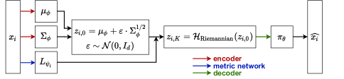
(a)

Figure 1: Geometry-aware VAE framework. Neural networks are highlighted with the colored arrows and $\mathcal{H}_{\mathrm{Riemannian}}$ are the normalizing flows using Riemannian Hamiltonian equations.

3.2.5 Discussion on the Posterior Expressiveness

Theoretically, using geometry-aware Hamiltonian normalizing flows should conduct to a better estimate of the true posterior $p_{\theta}(z|x)$ and so a better ELBO leading to a potentially higher likelihood $p_{\theta}(x)$. To validate this empirically, we report the estimated log-likelihood computed using Importance Sampling with the approximate posterior and Eq. (2) and Eq. (7). We use 100 importance samples and compute it three times on MNIST test set. Hamiltonian based models use 3 leapfrog steps. We also report the value of the ELBO and compute $D_{KL}(q_{\phi}(z|x)\lVert p_{\theta}(z|x))$. As shown in Table I, using geometry-aware normalizing flows leads to a higher estimated $p_{\theta}$ and a smaller gap between the estimated true posterior $p_{\theta}(z|x)$ and the variational approximation $q_{\phi}(z|x)$ measured by the KL divergence between both distributions. Note that all models are trained with the same architectures and training settings.

TABLE I: Effect of geometrical considerations on the estimated log-likelihood and ELBO on MNIST test set.

Model	$\log p_{\theta}(x)$ $\uparrow$	ELBO	$D_{KL}(q_{\phi}(z|x)\lVert p_{\theta}(z|x))$ $\downarrow$
VAE	-92.94 (0.01)	-100.06 (0.09)	7.12 (0.09)
HVAE	-85.33 (0.01)	-88.93 (0.02)	3.61 (0.02)
RHVAE	-82.64 (0.01)	-86.21 (0.04)	3.57 (0.03)

3.2.6 Sampling from the Latent Space

In this paper, we propose to amend the standard sampling procedure of classic VAEs after training to better exploit the Riemannian structure of the latent space. The geometry-aware VAE is indeed here seen as a tool able to capture the intrinsic latent structure of the data and so we propose to exploit this property directly within the generation procedure. This differs greatly from the standard fully probabilistic view where the prior distribution is used to generate new data. We believe that such an approach remains far from being optimal when one considers small data sets since, depending on its choice, the prior may either poorly prospect the latent space or sample in locations without any usable information. In that respect, our approach can be seen as part of the recently proposed prior learning based methods or methods relying on ex-post density estimation discussed earlier. Some of these methods were indeed proposed on the ground that there may exist a mismatch between the chosen prior distribution $p(z)$ and the optimal one given by the the aggregated posterior distribution $q(z)=\mathbb{E}_{x\sim p_{\mathrm{data}}(x)}[q_{\phi}(z|x)]$ [53, 85, 64, 63], where $p_{\mathrm{data}}(x)$ is the empirical distribution of the data [56]. Moreover, since our method is mainly about increasing the expressiveness of the variational posterior $q_{\phi}$ there exists no apparent reason that the latent codes are distributed according to the prior either. However, instead of learning a prior, we propose to directly use the metric that provides information on the geometry of the latent space as discussed and illustrated in Sec. 3.2.7 and Sec. 3.3. We indeed propose to sample from the following distribution:

$$p(z)=\frac{\mathbf{1}_{S}(z)\sqrt{\det\mathbf{G}^{-1}(z)}}{\int\limits_{\mathbb{R}^{d}}\mathbf{1}_{S}(z)\sqrt{\det\mathbf{G}^{-1}(z)dz}}\,,$$ (9)

where $S$ is a compact set so that the integral is well defined. Fortunately, since we use a parametrized metric given by Eq. (8) and whose inverse has a closed form, it is pretty straightforward to evaluate the numerator of Eq. (9). Then, classic MCMC sampling methods can be employed to sample from $p$ on $\mathbb{R}^{d}$. In this paper, we propose to use the Hamiltonian Monte Carlo (HMC) sampler [86] since the gradient of the log-density is computable. We provide some additional details in Appendix C.

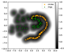
(a)

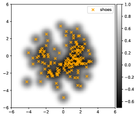
(b)

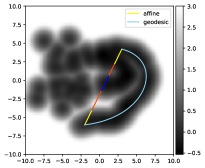
(c)

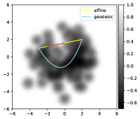
(d)

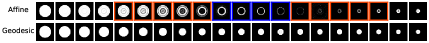
(e)

(f)

Figure 2: Geodesic interpolations under the learned metric in two different latent spaces. Top: Latent spaces with the log metric volume element presented in gray scale. Second row: The resulting interpolations under the Euclidean metric or the Riemannian metric. Third row: The learned manifolds and corresponding decoded samples. Bottom: Decoded samples all along the interpolation curves.

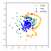
(a) Vanilla VAE

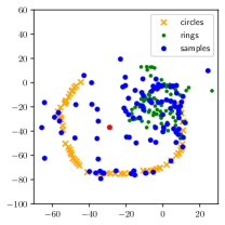
(b) VAE - VAMP prior

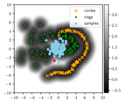
(c) Geometry-aware VAE - $\mathcal{N}(0,I_{d})$

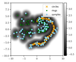
(d) Geometry-aware VAE - Ours

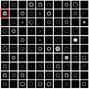
(e)

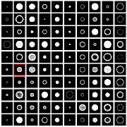
(f)

(g)

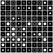
(h)

Figure 3: VAE sampling comparison. Top: The learned latent space along with the means $\mu_{\phi}(x_{i})$ of the latent code distributions (colored dots and crosses) and 100 latent space samples (blue dots) using either the prior distribution or the proposed scheme. For the geometry-aware VAEs, the log metric volume element is presented in gray scale in the background. Bottom: The 100 corresponding decoded samples in the data space.

3.2.7 Discussion on the Sampling Distribution

One may wonder what is the rationale behind the use of the distribution $p$ formerly defined in Eq. (9). By design, the metric is such that the metric volume element $\sqrt{\det\mathbf{G}(z)}$ is scaled by the factor $\lambda$ far from the encoded data points. Hence, choosing a relatively small $\lambda$ imposes that shortest paths travel through the most populated area of the latent space, i.e. next to the latent codes. As such, the metric volume element can be seen as a way to quantify the amount of information contained at a specific location of the latent space. The smaller the volume element the more information we have access to. Fig. 2 illustrates well these aspects. On the first row are presented two learned latent spaces along with the log of the metric volume element displayed in gray scale for two different data sets. The first one is composed of 180 binary disks and rings of different diameters and thicknesses while the second one is composed of 160 samples extracted from the FashionMNIST data set [87]. The means $\mu_{\phi}(x_{i})$ of the distributions associated with the latent variables are presented with the crosses and dots for each class. As expected, the metric volume element is smaller close to the latent variables since small $\lambda$’s were considered ($10^{-3}$ resp. $10^{-1}$). A common way to study the learned Riemannian manifold consists in finding geodesic curves, i.e. the shortest paths with respect to the learned Riemannian metric. Hence, on the second row of Fig. 2, we compare two types of interpolation in each latent space. For each experiment, we pick two points in the latent space and perform either a linear or a geodesic interpolation (i.e. using the Riemannian metric). The bottom row illustrates the decoded samples all along each interpolation curve. The first outcome of such an experiment is that, as expected, geodesic curves travel next to the codes and so do not explore areas of the latent space with no information whereas linear interpolations do. Therefore, decoding along geodesic curves produces far better and more meaningful interpolations in the input data space since in both cases we clearly see the starting sample being progressively distorted until the path reaches the ending point. This allows for instance interpolating between two shoes and keep the intrinsic topology of the data all along the path since each decoded sample on the interpolation curve looks like a shoe. This is made impossible under the Euclidean metric where shortest paths are straight lines and so may travel through areas of least interest. For instance, the affine interpolation travels through areas with no latent data and so produces decoded samples that are mainly a superposition of samples (see the red lines and corresponding decoded samples framed in red) or crosses areas with codes belonging to the other class (see the blue line and the corresponding blue frames). This study demonstrates that most of the information in the latent space is contained next to the codes and so, if we want to generate new samples that look-like the input data, we need to sample around them and that is why we elected the distribution in Eq. (9). Noteworthy is the fact that likewise [63], the prior $\mathcal{N}(0,I_{d})$ is now only reduced to a latent code regularizer during training ensuring that the covariances do not collapse to $0_{d}$ and the codes remains close to the origin and is never used to generate samples.

3.3 Generation Comparison

In this section, we propose to compare the new generation procedure with other generation methods in the context of low sample size data sets.

3.3.1 Qualitative Comparison

First, we validate the proposed generation method on a hand-made synthetic data set composed of 180 binary disks and rings of different diameters and thicknesses (see Appendix E). We then train 1) a vanilla VAE, 2) a VAE with VAMP prior [56], 3) a geometry-aware VAE but using the prior to generate and 4) a geometry-aware VAE with the proposed generation scheme, and compare the generated samples. Each model is trained until the ELBO does not improve for 20 epochs and any relevant parameter setting is made available in Appendix D. In Fig. 3, we compare the sampling obtained with each model. The first row shows the learned latent spaces along with the means of the encoded training data points for each class (crosses and dots) and 100 samples issued by the generation methods (blue dots). For the RHVAE models, the log metric volume element $\sqrt{\det\mathbf{G}}$ is also displayed in gray scale in the background. The bottom row shows the resulting 100 decoded samples in the data space.

The first outcome of this experiment is that sampling from the prior distribution leads to a quite poor latent space prospecting. This drawback is very well illustrated when a standard Gaussian distribution is used to sample from the latent space (see 1^st and 3^rd column of the 1^st row). The prior distribution having a higher mass close to zero will insist on latent samples close to the origin. Unfortunately, in such a case, latent codes close to the origin only belong to a single class (rings). Therefore, even though the number of training samples was roughly the same for disks and rings, we end up with a model over-generating samples belonging to a certain class (rings) and even to a specific type of data within this very class. This undesirable effect seems even ten-folded when considering the geometry-based VAE model since adding MCMC steps in the training process, as explained in Fig. 1, tends to stretch the latent space. It can be nonetheless noted that using a multi-modal prior such as the VAMP prior mitigates this and allows for a better prospecting. However, such a model remains hard to fit when trained with small data sets as it may overfit (resp. underfit) the training samples if the number of pseudo-inputs is too high (resp. low). Another limitation of prior-based generation methods lies in their inability to assess a given sample quality. They may indeed sample in areas of the latent space containing very few information and so conduct to generated samples that are meaningless. This appears even more striking when small data sets are considered. An interesting observation that was noted among others in [80] is that neural networks tend to interpolate very poorly in unseen locations (i.e. far from the training data points). When looking at the decoded latent samples (bottom row of Fig. 3) we eventually end up with the same conclusion. Actually, it appears that the networks interpolate quite linearly between the training data points in our case. This may be illustrated for instance by the red dots in the latent spaces in Fig. 3 whose corresponding decoded sample is framed in red. The sample is located between two classes and when decoded it produces an image mainly corresponding to a superposition of samples belonging to different classes. This aspect is also supported by the observations made when discussing the relevance of geodesic interpolations on Fig. 2 of Sec. 3.2.7. Therefore, these drawbacks may conduct to a (very) poor representation of the actual data set diversity while presenting quite a few irrelevant samples. Obviously the notion of irrelevance is here disputable but if the objective is to represent a given set of data we expect the generated samples to be close to the training data while having some specificities to enrich it. Impressively, sampling against the inverse of the metric volume element as proposed in Sec. 3.2.6 allows for a far more meaningful sample generation. Furthermore, the new sampling scheme avoids regions with no latent code, which thus contain poor information, and focuses on areas of interest so that almost every decoded sample is visually satisfying. Similar effects are observed on reduced versions of EMNIST [88], MNIST [89] and FashionMNIST data sets and higher dimensional latent spaces (dimension 10) where samples are most of the time degraded when the classic generation is employed while the new one allows the generation of more diverse and sharper samples (see Appendix E). Finally, the proposed method does not overfit the train data since the samples are not located on the centroids. The quantitative metrics of the next section also support this point.

TABLE II: GAN-train (the higher the better) and GAN-test (the closer to the baseline the better) scores. A benchmark DenseNet model is trained with five independent runs on the generated data $\mathcal{S}_{g}$ (resp. the real train set $\mathcal{S}_{\mathrm{train}}$) and tested on the real test set $\mathcal{S}_{\mathrm{test}}$ (resp. $\mathcal{S}_{g}$) to compute the GAN-train (resp. GAN-test) score. 1000 synthetic samples per class are considered for $\mathcal{S}_{g}$ so that it matches the size of $\mathcal{S}_{\mathrm{test}}$.

	reduced MNIST		reduced MNIST		reduced EMNIST
	(balanced)		(unbalanced)
Metric	GAN-train	GAN-test	GAN-train	GAN-test	GAN-train	GAN-test
Baseline	$90.6\pm 1.2$	-	$82.8\pm 0.7$	-	$84.5\pm 1.3$	-
VAE - $\mathcal{N}(0,I_{d})$	$83.4\pm 2.4$	$67.1\pm 4.9$	$74.7\pm 3.2$	$52.8\pm 10.6$	$75.3\pm 1.4$	$54.5\pm 6.5$
VAMP	$72.8\pm 6.7$	$77.6\pm 4.8$	$68.2\pm 6.6$	$76.7\pm 11.0$	$70.7\pm 8.0$	$69.0\pm 6.4$
VAE - GMM	$82.9\pm 2.4$	$76.5\pm 8.9$	$74.4\pm 3.8$	$68.4\pm 12.3$	$74.0\pm 2.6$	$57.6\pm 4.6$
RAE - GMM(2)	$90.8\pm 3.0$	$91.7\pm 1.9$	$85.5\pm 1.3$	$83.8\pm 6.2$	$80.3\pm 1.5$	$69.8\pm 7.2$
RAE - GMM(10)	$90.3\pm 2.3$	$\underline{95.3}\pm 1.6$	$81.0\pm 4.4$	$\underline{93.3}\pm 3.2$	$80.6\pm 1.6$	$83.4\pm 4.8$
RAE - GMM(20)	$\boldsymbol{91.1\pm 1.6}$	$\underline{96.6}\pm 1.5$	$84.3\pm 1.7$	$\underline{95.4}\pm 3.1$	$79.5\pm 1.1$	$\boldsymbol{85.0\pm 4.8}$
2-stage VAE	$84.8\pm 2.3$	$71.4\pm 8.3$	$80.8\pm 2.7$	$60.2\pm 9.2$	$79.6\pm 2.3$	$55.9\pm 3.9$
RHVAE - $\mathcal{N}(0,I_{d})$	$82.0\pm 2.9$	$63.1\pm 4.1$	$69.3\pm 1.8$	$46.9\pm 8.4$	$73.6\pm 4.1$	$55.6\pm 5.0$
Ours	$90.1\pm 1.4$	$\boldsymbol{88.1\pm 2.7}$	$\boldsymbol{86.2\pm 1.8}$	$\mathbf{83.8\pm 4.0}$	$\boldsymbol{82.6\pm 1.3}$	$76.0\pm 4.0$

3.3.2 Quantitative Comparison

In order to compare quantitatively the diversity and relevance of the samples generated by a generative model, several metrics were proposed [90, 91, 92, 93]. Since they suffer from some drawbacks [94, 95], we decide to use the GAN-train / GAN-test measure discussed in [94] as it appears to us well suited to measure the ability of a generative model to perform data augmentation. These two metrics consist in comparing the accuracy of a benchmark classifier trained on a set of generated data $\mathcal{S}_{g}$ and tested on a set of real images $\mathcal{S}_{\mathrm{test}}$ (GAN-train) or trained on the original train set $\mathcal{S}_{\mathrm{train}}$ (real images used to train the generative model) and tested on $\mathcal{S}_{g}$ (GAN-test). Those accuracies are then compared to the baseline accuracy given by the same classifier trained on $\mathcal{S}_{\mathrm{train}}$ and tested on $\mathcal{S}_{\mathrm{test}}$. These two metrics are quite interesting for our application since the first one (GAN-train) measures the quality and diversity of the generated samples (the higher the better) while the second one (GAN-test) accounts for the generative model’s tendency to overfit (a score significantly higher than the baseline accuracy means overfitting). Ideally, the closer to the baseline the GAN-test score the better. To stick to our low sample size setting, we compute these scores on three data sets created by down-sampling well-known databases. The first data set is created by extracting 500 samples from MNIST ensuring balanced classes (reduced MNIST). For the second one, 500 samples of the MNIST database are again considered but a random split is applied such that some classes are under-represented (reduced unbalanced MNIST). The last one consists in selecting 500 samples from 10 classes of the EMNIST data set having both lowercase and uppercase letters (reduced EMNIST) so that we end up with a small database with strong variability within classes. The balance matches the one in the initial data set (by merge). These three data sets are then divided into a baseline train set $\mathcal{S}_{\mathrm{train}}$ (80%) and a validation set $\mathcal{S}_{\mathrm{val}}$ (20%) used for the classifier training. Since the initial databases are huge, we use the original test set for $\mathcal{S}_{\mathrm{test}}$ so that it provides statistically meaningful results. For this comparison, we add a regularized autoencoder (RAE) [63], a 2-stage VAE [85] and a VAE where we use a 10-components mixture of Gaussian (GMM) instead of the prior to generate [63], to the models presented in Sec. 3.3.1. Each model is then trained on each class of $\mathcal{S}_{\mathrm{train}}$ to generate 1000 samples per class and $\mathcal{S}_{g}$ is created for each VAE by gathering all generated samples. A benchmark classifier chosen as a DenseNet [97] is then 1) trained on $\mathcal{S}_{\mathrm{train}}$ and tested on $\mathcal{S}_{\mathrm{test}}$ (baseline); 2) trained on $\mathcal{S}_{g}$ and tested on $\mathcal{S}_{\mathrm{test}}$ (GAN-train) and 3) trained on $\mathcal{S}_{\mathrm{train}}$ and tested on $\mathcal{S}_{g}$ (GAN-test) until the loss does not improve for 50 epochs on $\mathcal{S}_{\mathrm{val}}$. For each experiment, the model is trained five times and we report the mean score and the associated standard deviation in Table II. For the RAE we use a GMM and indicate the number of components between parentheses. As expected, the proposed method allows producing samples that are far more meaningful and relevant, in particular to perform DA. This is first illustrated by the GAN-train scores that are either very close to the accuracy obtained with the baseline or higher (see MNIST (unbalanced) in Table II). The fact that we are able to enhance the classifier’s accuracy even when trained only with synthetic data is very encouraging. Firstly, it proves that the created samples are close to the real ones and so we were able to capture the true distribution of the data. Secondly, it shows that we do not overfit the initial training data since we are able to add some relevant information through the synthetic samples. This last observation is also supported by the GAN-test scores for the proposed method which are quite close to the accuracies achieved on the baseline. In case of overfitting, the GAN-test score would be significantly higher than the baseline since the classifier is tested on the generated samples while trained on the real data that were also used to train the generative model. This is for instance the case for the RAE (underlined scores) where the number of components in the GMM impacts greatly the GAN-test metric. Having a score close to the baseline illustrates that the generative model is able to capture the distribution of the data and does not only memorize it [94]. Finally, this study again shows the relevance of considering new ways to generate data from VAEs, such as fitting a mixture of Gaussian in the latent space, using a 2-stage VAE or using the proposed method, as they all improve in almost all cases the metrics when compared to prior-based methods (lines 2 and 9 of Table II).

4 Data Augmentation: Evaluation and Robustness

In this section we show the relevance of the proposed improvements to perform data augmentation in a HDLSS setting through a series of experiments.

4.1 Setting

The setting we employ for DA consists in selecting a data set and splitting it into a train set (the baseline), a validation set and a test set. The baseline is then augmented using the proposed VAE framework and generation procedure. The generated samples are finally added to the original train set (i.e. the baseline) and fed to a classifier. The whole data augmentation procedure is illustrated in Fig. 4.

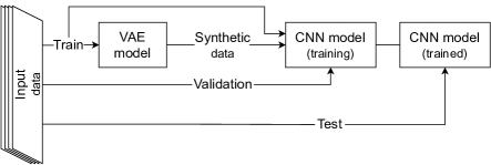
(a)

Figure 4: Overview of the data augmentation procedure. The input data set is divided into a train set (the baseline), a validation set and a test set. The train set is augmented using the VAE framework and generated data are then added to the baseline to train a benchmark classifier.

4.2 Toy Data Sets

The proposed VAE framework is here used to perform DA on several down-sampled well-known databases such that only tens of real training samples per class are considered so that we stick to the low sample size setting. First, the robustness of the method across these data sets is tested with a standard benchmark classifier. Then, its reliability across other common classifiers is stressed. Finally, its scalability to larger data sets and more complex models is discussed.

4.2.1 Materials

In this section, we use the same three data sets described in Sec. 3.3.2 and add one using the FashionMNIST data set and three classes we find hard to distinguish (i.e. T-shirt, dress and shirt). The data set is composed of 300 samples ensuring balanced classes (reduced Fashion). Finally, we also select 150 samples from three balanced classes of CIFAR10 [98] hard to classify (cat, dog and horse). In summary, we built five data sets having different class numbers, class splits and sample sizes. These data sets are again pre-processed such that 80% is allocated for training (referred to as the Baseline) and 20% for validation. Since the original data sets are huge, we use the test set provided in the original databases (e.g. $\approx$1000 samples per class for MNIST) so that it provides statistically meaningful results while allowing for a reliable assessment of the model’s generalization power on unseen data.

4.2.2 Robustness Across Data Sets

TABLE III: Data augmentation with a DenseNet model as benchmark. Mean accuracy and standard deviation across five independent runs are reported. The first three rows (Aug.) correspond to basic transformations (noise, crop, etc.). In gray are the cells where the accuracy is higher on synthetic data than on the baseline (i.e. the raw data). The test set is the one proposed in the entire original data set (e.g. $\approx$1000 samples per class for MNIST) so that it provides statistically meaningful results and allows for a good assessment of the model’s generalization power.

	MNIST	MNIST	EMNIST	FASHION	CIFAR	MNIST	MNIST	EMNIST	FASHION	CIFAR
		(unbal.)	(unbal.)				(unbal.)	(unbal.)
	Baseline + Synthetic					Synthetic Only
Baseline	$89.9/0.6$	$81.5/0.7$	$82.6/1.4$	$76.0/1.5$	$42.6/7.6$	-	-	-	-	-
Aug. (X5)	$92.8/0.4$	$86.5/0.9$	$85.6/1.3$	$77.5/2.0$	$47.7/2.3$	-	-	-	-	-
Aug. (X10)	$88.2/2.2$	$82.0/2.4$	$85.7/0.3$	$79.2/0.6$	$48.2/1.7$	-	-	-	-	-
Aug. (X15)	$92.8/0.7$	$85.8/3.4$	$86.6/0.8$	$80.0/0.5$	$48.0/2.2$	-	-	-	-	-
VAE - 200	$88.5/0.9$	$84.0/2.0$	$81.7/3.0$	$78.6/0.4$	$46.9/1.3$	$69.9/1.5$	$64.6/1.8$	$65.7/2.6$	$73.9/3.0$	$40.5/4.1$
VAE - 1k	$91.2/1.0$	$86.0/2.5$	$84.3/1.6$	$77.6/2.1$	$47.7/1.4$	$83.4/2.4$	$74.7/3.2$	$75.3/1.4$	$71.4/6.1$	$41.3/2.4$
VAMP - 200	$91.4/1.9$	$81.1/2.7$	$84.2/0.8$	$79.8/0.8$	$45.6/6.9$	$61.3/3.2$	$52.4/3.0$	$67.4/1.4$	$70.4/3.2$	$40.6/6.6$
VAMP - 1k	$\boldsymbol{93.6/0.9}$	$88.0/1.1$	$86.2/1.1$	$79.6/0.4$	$45.2/6.1$	$72.8/6.7$	$68.2/6.6$	$70.7/8.0$	$69.2/5.4$	$39.7/7.7$
RHVAE - 200∗	$89.9/0.5$	$82.3/0.9$	$83.0/1.3$	$77.6/1.3$	$45.2/1.9$	$76.0/1.8$	$61.5/2.9$	$59.8/2.6$	$72.8/3.6$	$42.4/1.2$
RHVAE - 1k∗	$91.7/0.8$	$84.7/1.8$	$84.7/2.4$	$79.3/1.6$	$42.1/2.9$	$82.0/2.9$	$69.3/1.8$	$73.6/4.1$	$76.0/4.1$	$40.7/3.2$
VAE GMM - 200	$90.5/1.1$	$82.9/2.2$	$84.8/1.0$	$79.6/0.7$	$44.9/1.9$	$76.5/1.5$	$64.0/2.6$	$70.5/1.5$	$71.9/2.2$	$38.7/4.2$
VAE GMM - 1k	$92.0/1.8$	$86.7/1.0$	$86.1/1.1$	$79.5/0.7$	$38.9/2.4$	$82.9/2.4$	$74.4/3.8$	$74.0/2.6$	$73.9/2.5$	$41.6/2.7$
2-stage VAE - 200	$91.2/1.2$	$83.5/1.5$	$85.3/1.9$	$\boldsymbol{80.5/0.6}$	$44.4/2.3$	$82.3/1.1$	$74.9/2.3$	$76.7/1.3$	$76.2/2.0$	$38.1/2.6$
2-stage VAE - 1k	$93.3/0.7$	$87.7/2.4$	$86.7/1.1$	$79.5/0.9$	$38.8/3.0$	$84.8/2.3$	$80.8/2.7$	$79.6/2.3$	$75.8/1.8$	$37.9/3.6$
RAE - 200	$91.6/1.1$	$81.3/1.3$	$85.2/0.9$	$80.1/0.8$	$46.2/2.9$	$83.6/2.8$	$74.5/1.6$	$76.9/1.6$	$66.5/4.4$	$33.7/1.7$
RAE - 1k	$93.3/0.8$	$88.3/1.1$	$85.8/0.9$	$79.8/1.3$	$44.1/2.6$	$\pagecolor{gray!30}\boldsymbol{90.3/2.3}$	$81.0/4.4$	$80.6/1.6$	$62.0/5.1$	$33.6/0.4$
Ours - 200	$91.0/1.0$	$84.1/2.0$	$85.1/1.1$	$77.0/0.8$	$46.8/2.2$	$87.2/1.1$	$79.5/1.6$	$77.0/1.6$	$\pagecolor{gray!30}77.0/0.8$	$\pagecolor{gray!30}\boldsymbol{47.3/1.7}$
Ours - 1k	$93.2/0.8$	$\mathbf{89.7/0.8}$	$\boldsymbol{87.0/1.0}$	$80.2/0.8$	$\boldsymbol{49.2/2.3}$	$\pagecolor{gray!30}90.1/1.4$	$\pagecolor{gray!30}\boldsymbol{86.2/1.8}$	$\pagecolor{gray!30}\boldsymbol{82.6/1.3}$	$\pagecolor{gray!30}\boldsymbol{79.3/0.6}$	$\pagecolor{gray!30}46.7/3.1$

The first experiment we conduct consists in assessing the method’s robustness across the five aforementioned data sets. For this study, we propose to consider a DenseNet model as benchmark classifier. On the one hand, the training data (the baseline) is augmented by a factor 5, 10 and 15 using classic data augmentation methods (random noise, random crop, rotation, etc.) so that the proposed method can be compared with classic and simple augmentation techniques. On the other hand, the protocol described in Fig. 4 is employed with the same VAEs as before. The generative models are trained individually on each class of the baseline until the ELBO does not improve for 20 epochs. The VAEs are then used to produce 200 or 1000 new synthetic samples per class using the same generation protocols as described in Sec. 3.3.2. Finally, the benchmark DenseNet model is trained with five independent runs on either 1) the baseline, 2) the augmented data using classic augmentation methods, 3) the augmented data using the VAEs or 4) only the synthetic data created by the generative models. For each experiment, the mean accuracy and the associated standard deviation across those five runs are reported in Table III. An early stopping strategy is employed and CNN training is stopped if the loss does not improve on the validation set for 50 epochs.

The first outcome of such a study is that, as expected, generating synthetic samples with the proposed method seems to enhance their relevance in particular for data augmentation tasks. This is for instance illustrated by the first column of Table III where synthetic samples are added to the baseline. While adding samples generated either by a VAE or RHVAE and using the prior distribution seems to improve the classifier accuracy when compared with the baseline, the gain remains limited since it struggles to exceed the gain reached with classic augmentation methods. On the contrary, methods using either more complex priors (VAMP), a second VAE or a GMM allow improving classification results on MNIST and Fashion but still under-perform on EMNIST and CIFAR. Finally, the proposed generation method is able to produce very useful samples for the CNN model since in all cases it allows the classifier to either achieve the best result (highlighted in bold) or comparable performance than peers while keeping a relatively low standard deviation. Secondly, the relevance of the samples produced by the proposed scheme is even more supported by the second column of Table III where the classifier is trained only using the synthetic samples generated by the VAEs. First, even with a quite small number of samples generated with our method (200 per class), the classifier is almost able to reach the accuracy achieved with the baseline. For instance, when the CNN is trained on reduced MNIST with 200 synthetic samples per class generated with our method, it is able to achieve an accuracy of 87.2% vs. 89.9% with the baseline. In comparison, any other method fails to produce meaningful samples since a quite significant loss in accuracy is observed. The fact that the classifier almost performs as well on the synthetic data as on the baseline is good news since it shows that the proposed framework is able to produce samples accounting for the original data set diversity even with a small number of generated samples. Even more interesting, as the number of synthetic data increases, the classifier is able to perform much better on the synthetic data than on the baseline since a gain of 3 to 6 points in accuracy is observed. Again, this strengthens the observations made in Sec. 3.3.1 and 3.3.2 where we noted that the proposed method is able to enrich the initial data set with relevant and realistic samples.

Finally, it can be seen in this experiment why geometric data augmentation methods are still questionable and remain data set dependent. For example, augmenting the baseline by a factor 10 (where we add flips and rotations on the original data) seems to have no significant effect on the reduced MNIST data sets while it still improves results on reduced EMNIST, Fashion and CIFAR. We see here how the expert knowledge comes into play to assess the relevance of the transformations applied to the data. Fortunately, the method we propose does not require such knowledge and appears to be quite robust to data set changes.

4.2.3 Robustness Across Classifiers

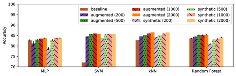
(a) reduced MNIST balanced

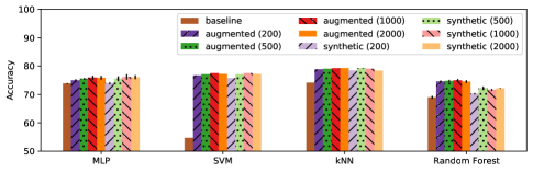
(b) reduced MNIST unbalanced

Figure 5: Evolution of the accuracy of four benchmark classifiers on reduced balanced MNIST (left) and reduced unbalanced MNIST data sets (right). Stochastic classifiers are trained with five independent runs and we report the mean accuracy and standard deviation on the test set.

In addition to assessing the robustness of the method to data sets changes, we also propose to evaluate its reliability across classifiers. To do so, we consider very different common supervised classifiers: a multi layer perceptron (MLP) [3], a random forest [99], the $k$-NN algorithm and a SVM [100]. Each of the aforementioned classifiers is again trained either on 1) the original training data set (the baseline); 2) the augmented data using the proposed method and 3) only the synthetic data generated by our method with five independent runs and using the same data sets as presented in Sec. 4.2.1. Finally, we report the mean accuracy and standard deviation across these runs for each classifier and data set. The results for the balanced (resp. unbalanced) reduced MNIST data set can be found in Fig. 5a (resp. Fig. 5b). Metrics obtained on reduced EMNIST and Fashion are available in Appendix F but reflect the same tendency.

As illustrated in Fig. 5, the method appears quite robust to classifier changes as well since it allows improving the model’s accuracy significantly for almost all classifiers (the accuracy achieved on the baseline is represented by the leftmost bar in Fig. 5 for each classifier). The method’s strength is even more striking when unbalanced data sets are considered since the method is able to produce meaningful samples even with a very small number of training data and so it is able to over-sample the minority classes in a reliable way. Moreover, as observed earlier, synthetic samples are again helpful to enhance classifiers’ generalization power since they perform better when trained only on synthetic data than on the baseline in almost all cases.

4.2.4 A Note on the Method Scalability

Finally, we also discuss the method scalability to larger data sets, bigger models and higher dimensional latent spaces. To do so, we consider the MNIST data set and a benchmark classifier taken as a DenseNet which performs well on such data. First, we down-sample the original MNIST database in order to progressively decrease the number of samples per class. We start by creating a data set having 1000 samples per class to finally reach 20 samples per class. For each created data set, we allocate 80% for training (the baseline) and reserve 20% for the validation set. A geometry-aware VAE is then trained on each class of the baseline until the ELBO does not improve for 50 epochs and is used to generate synthetic samples (12.5$\times$ the baseline). The benchmark CNN is trained with five independent runs on either 1) the baseline, 2) the augmented data or 3) only the synthetic data generated with our model. The evolution of the mean accuracy on the original test set ($\approx$1000 samples per class) according to the number of samples per class is presented in Fig. 6 (left). Second, we only consider 50 samples per class and train the VAE on each class to generate 1000 samples per class. The number of the classifier’s parameters is also progressively changed and we report the mean accuracy of the CNN according to the number of parameters in Fig. 6 (middle). Finally, we consider several latent space dimensions for the VAE ranging from 2 to 50 and plot the evolution of the CNN accuracy according the latent space dimension (right).

First, this experiment shows that the fewer samples in the training set, the more useful the method appears. Using the proposed augmentation framework indeed allows for a gain of more than 9.0 points in the CNN accuracy when only 20 samples per class are considered. In other words, as the number of samples increases, the marginal gain seems to decrease. Nevertheless, this reduction must be put into perspective since it is commonly acknowledged that, as the results on the baseline increase (and thus get closer to the perfect score), it is even more challenging to improve the score with the augmented data. In this experiment, we are nonetheless still able to improve the model accuracy even when it already achieves a very high score. For instance, with 500 samples per class, the augmentation method still allows increasing the model accuracy from 97.7% to 98.8%. Finally, for data sets with fewer than 500 samples per class, the classifier is able to outperform the baseline even when trained only with the synthetic data. This shows again the strong generalization power of the proposed method which allows creating new relevant data for the classifier. Another interesting take from these experiments is that the augmentation method seems to benefit both simple and more complex models since the gain in the model accuracy remains quite steady ($\approx$ 3 pts) regardless of the number of parameters in the classifier (Fig. 6 (middle)). Finally, the impact of the dimension of the latent space remains limited for such a framework as the classification accuracy remains stable. Nonetheless, this may be due to the simplicity of the database and more complex data might need higher dimensional latent spaces.

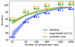
(a)

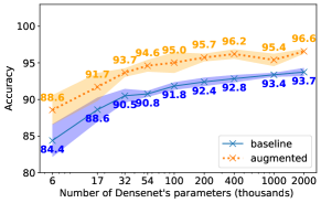
(b)

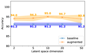
(c)

Figure 6: Evolution of the accuracy of a benchmark DenseNet classifier according to the number of samples in the train set (i.e. the baseline) (left), the number of parameters of the Densenet (middle) and the latent space dimension of the VAE (right) on MNIST. Curves show the mean accuracy and standard deviation across 5 runs on the original test set for the baseline (blue), the augmented data (orange) and the synthetic ones (green).

5 Validation on Medical Imaging

With this last series of experiments, we assess the validity of our data augmentation framework on a binary classification task consisting in differentiating Alzheimer’s disease (AD) patients from cognitively normal (CN) subjects based on T1-weighted (T1w) MR images of human brains. Such a task is performed using a CNN trained, as before, either on 1) real images, 2) synthetic samples or 3) both. In this section, label definition, preprocessing, quality check, data split and CNN training and evaluation is done using Clinica [101] and ClinicaDL [102], two open-source software packages for neuroimaging processing.

5.1 Data Augmentation Literature for AD vs CN Task

Even though many studies use CNNs to differentiate AD from CN subjects with anatomical MRI [103], we did not find any meta-analysis on the use of data augmentation for this task. Some results involving DA can nonetheless be cited and are presented in Table IV. However, assessing the real impact of data augmentation on the performance of the models remains challenging. For instance, this is illustrated by the works of [104] and [105], which are two examples in which DA was used and led to two significantly different results, although a similar framework was used in both studies. Interestingly, as shown in Table IV, studies using DA for this task only relied on simple affine and pixel-level transformations, which may reveal data dependent. Note that complex DA was actually performed for AD vs CN classification tasks on PET images, but PET is less frequent than MRI in neuroimaging data sets [106]. As noted in the previous sections, our method would apply pretty straightforwardly to this modality as well. For MRI, other techniques such as transfer learning [107] and weak supervision [108] were preferred to handle the small amount of samples in data sets and may be coupled with DA to further improve the classifier performance.

TABLE IV: Accuracy obtained by studies performing AD vs CN classification with CNNs applied on T1w MRI and using data augmentation

				Accuracy
Study	Methods	Subj.	Images	Baseline	Augmented
[109]	rotate, flip, shift	417	417	78.8	81.3
[110]	flip	340	1198	–	90.1
[111]	shift, sample, rotate	193	193	–	85.5
[104]	shift, blur, flip	720	720	82.8	83.7
[105]	shift, blur	720	720	–	90.0

5.2 Materials

Data used in this section were obtained from the Alzheimer’s Disease Neuroimaging Initiative (ADNI) database (adni.loni.usc.edu) and the Australian Imaging, Biomarkers and Lifestyle (AIBL) study (aibl.csiro.au).

The ADNI was launched in 2003 as a public-private partnership, led by Principal Investigator Michael W. Weiner, MD. The primary goal of ADNI has been to test whether serial MRI, PET, other biological markers, and clinical and neuropsychological assessment can be combined to measure the progression of mild cognitive impairment and early AD. For up-to-date information, see www.adni-info.org. The ADNI data set is composed of four cohorts: ADNI-1, ADNI-GO, ADNI-2 and ADNI-3. The data collection of ADNI-3 has not ended yet, hence our data set contains all images and metadata that were already available on May 6, 2019. Similarly to ADNI, the AIBL data set seeks to discover which biomarkers, cognitive characteristics, and health and lifestyle factors determine the development of AD. This cohort is also longitudinal and the diagnosis is given according to a series of clinical tests [112]. Data collection for this cohort is over.

Two diagnoses are considered for the classification task:

• CN: baseline session of participants who were diagnosed as cognitively normal at baseline and stayed stable during the follow-up;

• AD: baseline session of participants who were diagnosed as demented at baseline and stayed stable during the follow-up.

Table V summarizes the demographics, the mini-mental state examination (MMSE) and global clinical dementia rating (CDR) scores at baseline of the participants included in our data set. The MMSE and the CDR scores are classical clinical scores used to assess dementia. The MMSE score has a maximal value of 30 for cognitively normal persons and decreases if symptoms are detected. The CDR score has a minimal value of 0 for cognitively normal persons and increases if symptoms are detected.

TABLE V: Summary of participant demographics, mini-mental state examination (MMSE) and global clinical dementia rating (CDR) scores at baseline.

Data set	Label	Subj.	Age	Sex M/F	MMSE	CDR
ADNI	CN	403	$73.3\pm 6.0$	185/218	$29.1\pm 1.1$	0: 403
	AD	362	$74.9\pm 7.9$	202/160	$23.1\pm 2.1$	0.5: 169, 1: 192
						2: 1
AIBL	CN	429	$73.0\pm 6.2$	183/246	$28.8\pm 1.2$	0: 406, 0.5: 22
						1: 1
	AD	76	$74.4\pm 8.0$	33/43	$20.6\pm 5.5$	0.5: 31, 1: 36
						2: 7, 3: 2

5.3 Preprocessing of T1-Weighted MRI

The steps performed in this section correspond to the procedure followed in [103] and are listed below:

1. Raw data are converted to the BIDS standard [113],

2. Bias field correction is applied using N4ITK [114],

3. T1w images are linearly registered to the MNI standard space [115, 116] with ANTS [117] and cropped. This produced images of size 169$\times$208$\times$179 with 1 mm³ isotropic voxels.

4. An automatic quality check is performed using an open-source pretrained network [118]. All images passed the quality check.

5. NIfTI files are converted to tensor format.

6. (Optional) Images are down-sampled with a trilinear interpolation leading to a size of 84$\times$104$\times$89.

7. Intensity rescaling between the minimum and maximum values of each image is performed.

These steps lead to 1) down-sampled images (84$\times$104$\times$89) or 2) high-resolution images (169$\times$208$\times$179).

5.4 Evaluation Procedure

The ADNI data set is split into three sets: training, validation and test. First, the test set is created using 100 randomly chosen participants for each diagnostic label (i.e. 100 CN, 100 AD). The rest of the data set is split between the training (80%) and the validation (20%) sets. We ensure that age, sex and site distributions between the three sets are not significantly different.

A smaller training set (denoted as train-50) is extracted from the obtained training set (denoted as train-full). This set comprises only 50 images per diagnostic label, instead of 243 CN and 210 AD for train-full. We ensure that age and sex distributions between train-50 and train-full are not significantly different. This is not done for the site distribution as there are more than 50 sites in the ADNI data set (so they could not all be represented in this smaller training set). AIBL data are never used for training or hyperparameter tuning and are only used as an independent test set.

5.5 CNN Classifiers

A CNN takes as input an image and outputs a vector of size $C$ corresponding to the number of labels existing in the data set. Then, a CNN predicts the label of a given image by selecting the highest probability in the output vector.

5.5.1 Hyperparameter Choices

As for the VAE, the architecture of the CNN depends on the size of the input. Then, there is one architecture per input size: down-sampled images and high-resolution images (see Appendix D.4). Moreover, two different paradigms are used to choose the architecture. First, we reuse the same architecture as in [103]. This architecture was obtained by optimizing manually the networks on the ADNI data set for the same task (AD vs CN). A slight adaption is done for the down-sampled images, which consists in resizing the number of nodes in the fully-connected layers to keep the same ratio between the input and output feature maps in all layers. We denote these architectures as baseline. Secondly, we launch a random search [119] that allows exploring different hyperperameter values. The hyperparameters explored for the architecture are the number of convolutional blocks, of filters in the first layer and of convolutional layers in a block, the number of fully-connected layers and the dropout rate. Other hyperparameters such as the learning rate and the weight decay are also part of the search. 100 different random architectures are trained on the 5-fold cross-validation done on train-full. For each input, we choose the architecture that obtained the best mean balanced accuracy across the validation sets of the cross-validation. We denote these architectures as optimized.

5.5.2 Network Training

The weights of the convolutional and fully-connected layers are initialized as described in [120], which corresponds to the default initialization method in PyTorch. Networks are trained for 100 epochs for baseline and 50 epochs for optimized. The training and validation losses are computed with the cross-entropy loss. For each experiment, the final model is the one that obtained the highest validation balanced accuracy during training. The balanced accuracy of the model is evaluated at the end of each epoch.

5.6 Experimental Protocol

As done in the previous sections, we perform three types of experiments and train the model on 1) only the real images, 2) only on synthetic data and 3) on synthetic and real images. Due to the current implementation, augmentation on high-resolution images is not possible due to computational time and so these images are only used to assess the baseline performance of the CNN with the maximum information available. Each series of experiments is done once for each training set (train-50 and train-full). The CNN and the VAE share the same training set, and the VAE does not use the validation set during its training. For each training set, two VAEs are trained, one on the AD label only and the other on the CN label only. Examples of real and generated AD images are shown in Fig. 7. For each experiment 20 runs of the CNN training are launched. The use of a smaller training set train-50 allows mimicking the behavior of the framework on smaller data sets, which are frequent in the medical domain.

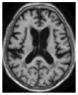
(a)

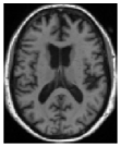
(b)

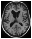
(c)

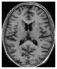
(d)

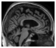
(e)

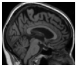
(f)

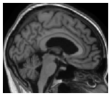
(g)

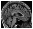
(h)

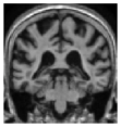
(i)

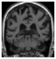
(j)

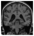
(k)

(l)

Figure 7: Example of two true patients compared to two generated by our method. Can you find the intruders ? Answers in Appendix H.

5.7 Results

Results presented in Table VI (resp. Table VII) are obtained with baseline (resp. optimized) hyperparameters and using either the train-full or train-50 data set. Scores on synthetic images only are given in Appendix I. Experiments are done on down-sampled images unless high-resolution is specified.

TABLE VI: Mean test performance of each series of 20 runs trained with the baseline hyperparameters

		ADNI			AIBL
training	data set	sensitivity	specificity	balanced	sensitivity	specificity	balanced
set				accuracy			accuracy
train-50	real	$70.3\pm 12.2$	$62.4\pm 11.5$	$66.3\pm 2.4$	$60.7\pm 13.7$	$73.8\pm 7.2$	$67.2\pm 4.1$
	real (high-resolution)	$78.5\pm 9.4$	$57.4\pm 8.8$	$67.9\pm 2.3$	$57.2\pm 11.2$	$75.8\pm 7.0$	$66.5\pm 3.0$
	500 synthetic + real	$71.9\pm 5.3$	$67.0\pm 4.5$	$69.4\pm 1.6$	$55.9\pm 6.8$	$81.1\pm 3.1$	$68.5\pm 2.5$
	2000 synthetic + real	$72.2\pm 4.4$	$70.3\pm 4.3$	$71.2\pm 1.6$	$66.6\pm 7.1$	$79.0\pm 4.1$	$72.8\pm 2.2$
	5000 synthetic + real	$\boldsymbol{74.7\pm 5.3}$	$\boldsymbol{73.5\pm 4.8}$	$\boldsymbol{74.1\pm 2.2}$	$\boldsymbol{71.7\pm 10.0}$	$80.5\pm 4.4$	$\boldsymbol{76.1\pm 3.6}$
	10000 synthetic + real	$74.7\pm 7.0$	$73.4\pm 6.1$	$74.0\pm 2.7$	$69.1\pm 9.9$	$\boldsymbol{80.7\pm 5.1}$	$74.9\pm 3.2$
train-full	real	$79.1\pm 6.2$	$76.3\pm 4.2$	$77.7\pm 2.5$	$70.6\pm 6.7$	$86.3\pm 3.6$	$78.4\pm 2.4$
	real (high-resolution)	$84.5\pm 3.8$	$76.7\pm 4.0$	$80.6\pm 1.1$	$71.6\pm 6.4$	$89.2\pm 2.7$	$80.4\pm 2.6$
	500 synthetic + real	$82.5\pm 3.4$	$81.9\pm 5.4$	$82.2\pm 2.4$	$76.0\pm 6.3$	$89.7\pm 3.3$	$82.9\pm 2.5$
	2000 synthetic + real	$\boldsymbol{85.4\pm 4.0}$	$86.4\pm 5.9$	$85.9\pm 1.6$	$77.2\pm 6.9$	$90.4\pm 3.8$	$83.8\pm 2.2$
	5000 synthetic + real	$84.6\pm 4.2$	$86.9\pm 3.6$	$85.7\pm 2.1$	$76.9\pm 5.2$	$\boldsymbol{91.4\pm 3.0}$	$84.2\pm 2.2$
	10000 synthetic + real	$84.2\pm 2.8$	$\boldsymbol{88.5\pm 2.9}$	$\boldsymbol{86.3\pm 1.8}$	$\boldsymbol{79.1\pm 4.7}$	$91.0\pm 2.6$	$\boldsymbol{85.1\pm 1.9}$

TABLE VII: Mean test performance of each series of 20 runs trained with the optimized hyperparameters

		ADNI			AIBL
training	image type	sensitivity	specificity	balanced	sensitivity	specificity	balanced
set				accuracy			accuracy
train-50	real	$75.4\pm 5.0$	$75.5\pm 5.3$	$75.5\pm 2.7$	$68.6\pm 8.5$	$82.6\pm 4.2$	$75.6\pm 4.1$
	real (high-resolution)	$73.6\pm 6.2$	$70.6\pm 5.9$	$72.1\pm 3.1$	$57.8\pm 12.3$	$84.6\pm 4.2$	$71.2\pm 5.1$
	500 synthetic + real	$73.2\pm 4.2$	$78.0\pm 3.3$	$75.6\pm 2.5$	$69.2\pm 9.4$	$\boldsymbol{82.7\pm 4.1}$	$76.0\pm 4.2$
	2000 synthetic + real	$75.2\pm 3.8$	$\boldsymbol{78.6\pm 4.4}$	$76.9\pm 2.4$	$77.8\pm 8.8$	$82.2\pm 4.5$	$80.0\pm 3.6$
	5000 synthetic + real	$77.1\pm 3.7$	$76.7\pm 4.1$	$76.9\pm 2.5$	$80.7\pm 6.1$	$81.2\pm 3.7$	$80.9\pm 2.7$
	10000 synthetic + real	$\boldsymbol{77.8\pm 4.6}$	$78.2\pm 4.9$	$\boldsymbol{78.0\pm 2.1}$	$\boldsymbol{81.7\pm 4.9}$	$81.9\pm 4.6$	$\boldsymbol{81.9\pm 2.2}$
train-full	real	$82.5\pm 4.2$	$88.5\pm 6.6$	$85.5\pm 2.4$	$75.1\pm 8.4$	$88.7\pm 9.0$	$81.9\pm 3.2$
	real (high-resolution)	$82.6\pm 4.5$	$88.9\pm 6.3$	$85.7\pm 2.5$	$78.9\pm 5.4$	$89.9\pm 4.0$	$84.4\pm 1.7$
	500 synthetic + real	$82.3\pm 2.3$	$89.8\pm 2.7$	$86.0\pm 1.8$	$74.9\pm 5.0$	$91.4\pm 2.6$	$83.2\pm 2.4$
	2000 synthetic + real	$\boldsymbol{83.1\pm 4.2}$	$\boldsymbol{91.3\pm 3.2}$	$\boldsymbol{87.2\pm 1.7}$	$76.0\pm 4.7$	$92.0\pm 2.4$	$84.0\pm 2.0$
	5000 synthetic + real	$81.9\pm 3.5$	$90.9\pm 2.5$	$86.4\pm 1.3$	$74.1\pm 4.9$	$\boldsymbol{92.9\pm 1.9}$	$83.5\pm 2.2$
	10000 synthetic + real	$82.2\pm 3.4$	$91.2\pm 3.6$	$86.7\pm 1.8$	$\boldsymbol{76.4\pm 4.2}$	$92.1\pm 2.1$	$\boldsymbol{84.3\pm 1.8}$

Even though the VAE augmentation is performed on down-sampled images, the classification performance is at least as good as that of the best baseline performance, or can greatly exceed it:

• train-50 and baseline model: balanced accuracy increases by 6.2 pts on ADNI and 8.9 pts on AIBL,

• train-full and baseline model: balanced accuracy increases by 5.7 pts on ADNI and 4.7 pts on AIBL,

• train-50 and optimized model: balanced accuracy increases by 2.5 pts on ADNI and 6.3 pts on AIBL,

• train-full and optimized model balanced accuracy increases by 1.5 pts on ADNI and -0.1 pts on AIBL.

Then, the performance increase thanks to DA is higher when using the baseline hyperparameters than the optimized ones. A possible explanation could be that the optimized network is already close to the maximum performance that can be reached with this setup and cannot be much improved with DA. Moreover, the VAE has not been subject to a similar search, which places it at a disadvantage. For both hyperparameters, the performance gain is higher on train-50 than on train-full, which supports the results obtained in the previous section (see Fig. 6). The baseline balanced accuracy with the baseline hyperparameters on train-full, 80.6% on ADNI and 80.4% on AIBL, are similar to the results of [103]. With DA, we improve our balanced accuracy to 86.3% on ADNI and 85.1% on AIBL: this performance is similar to their result using autoencoder pretraining (which can be very long to compute) and longitudinal data (1830 CN and 1106 AD images) instead of baseline data (243 CN and 210 AD images) as we did.

In each table, the first two rows display the baseline performance obtained on real images only. As expected, training on high-resolution images leads to a better performance than training on down-sampled images. This is not the case for the optimized network on train-50, which obtained a balanced accuracy of 72.1% on ADNI and 71.2% on AIBL with high-resolution images versus 75.5% on ADNI and 75.6% on AIBL with down-sampled images. This is explained by the fact that the hyperparameter choices are made on train-full and so there is no guarantee that they could lead to similar results with fewer data samples.

6 Discussion

Contrary to techniques that are specific to a field of application, our method produced relevant data for diverse data sets including 2D natural images (MNIST, EMNIST, Fashion and CIFAR) or 3D medical images (ADNI and AIBL). Moreover, we noted that the networks trained on ADNI gave similar balanced accuracies on the ADNI test subset and AIBL showing that our synthetic data learned on ADNI benefit in the same way AIBL, and that it did not overfit the characteristics of ADNI. In addition to the robustness across data sets, the relevance of synthetic data for diverse classifiers was assessed. For toy data, these classifiers were a MLP, a random forest, a k-NN algorithm and a SVM. On medical image data, two different CNNs were studied: a baseline one that has been only slightly optimized in a previous study and an optimized one found with a more extensive search (random search). All these classifiers performed best on augmented data than real data only. However, for medical image data, we noted that the data augmentation was more beneficial to the baseline network, than to the optimized one but both networks obtained a similar performance with data augmentation on the largest training set. This means that data augmentation could avoid spending time and/or resources optimizing a classifier. The ability of the model to generate relevant data and enrich the original training data was also supported by the fact that almost all classifiers could achieve a better classification performance when trained only on synthetic data than on the real train. The method scalability to larger data sets and more complex models was also discussed.

Our generation framework appears also very well suited to perform data augmentation in a HDLSS setting (the binary classification of AD and CN subjects using T1w MRI). In all cases, the classification performance was at least as good as the maximum performance obtained with real data and could even be much better. For instance, the method allowed the balanced accuracy of the baseline CNN to jump from 66.3% to 74.3% when trained with only 50 images per class and from 77.7% to 86.3% when trained with 243 CN and 210 AD while still improving greatly sensitivity and specificity metrics. We witnessed a greater performance improvement than the other studies using a CNN on T1w MRI to differentiate AD and CN subjects [109, 110, 111, 104, 105]. Indeed, these studies used simple transforms (affine and pixel-wise) that may not bring enough variability to improve the CNN performance. Though many complex methods now exist to perform data augmentation, they are still not widely adopted in the field of medical imaging. We suspect that this is mainly due to the lack of reproducibility of such frameworks. Hence we provide the source code, as well as scripts to easily reproduce the experiments of this paper from the ADNI and AIBL data set download to the final evaluation of the CNN performance. We also developed a software implementing the method and making it easily accessible to the community.

However, our classification performance on synthetic data could be improved in many ways. First, we chose in this study not to spend much time optimizing the VAE’s hyperparameters and so in Sec. 5 we chose to work with down-sampled images to deal with memory issues. We could look for another architecture to train the VAE directly on high-resolution images leading potentially to a better performance as witnessed in experiments on real images only. Moreover, we could couple the advantages of other techniques such as autoencoder pretraining or weak supervision to our data augmentation framework. However, the advantages may not stack as observed when using DA on optimized hyperparameters. Finally, we chose to train our networks with only one image per participant, but our framework could also benefit from the use of the whole follow-up of all patients to further improve performance. However, a long follow-up is rather an exception in the context of medical imaging. This is why we assessed the relevance of our DA framework in the context of small data sets which is a main issue in this field. Nonetheless, a training set of 50 images per class can still be seen as large in the case of rare diseases and so it may be interesting to evaluate the reliability of our method on even smaller training sets.

7 Conclusion

In this paper, we proposed a new VAE-based data augmentation framework whose performance and robustness were validated on classification tasks on toy and real-life data sets. This method relies on a model combining a proper latent space modeling of the VAE seen as a Riemannian manifold and a new generation procedure exploiting such geometrical aspects. In particular, the generation method does not use the prior as is standard since we showed that, depending on its choice and the data set considered, it may lead to a very poor latent space prospecting and a degraded sampling while the proposed method does not suffer from such drawbacks. The proposed amendments were motivated, discussed and compared to other VAE models and demonstrated promising results. The model indeed appeared to be able to generate new data faithfully and demonstrated a strong generalization power which makes it very well suited to perform data augmentation even in the challenging context of HDLSS data. For each augmentation experiment, it was able to enrich the initial data set so that a classifier performs better on augmented data than only on the real ones. Future work would consist in building a framework able to handle longitudinal data and so able to generate not only one image but a whole patient trajectory.

Clément Chadebec is a PhD student at Université de Paris and Inria and funded by $PR[AI]RIE$. His research interests include machine learning and in particular generative models along with Riemannian geometry and computational statistics for medicine. He received master degrees from Ecole Nationale des Mines de Paris and Ecole Normale Supérieure Paris-Saclay.

Elina Thibeau-Sutre is a PhD student at Sorbonne Université and Inria. Her research interest includes deep learning application to neuroimaging data, its interpretability and reproducibility. She received master degrees from Ecole Nationale des Mines de Paris and Ecole supérieure de physique et de chimie industrielles (Paris, France).

Ninon Burgos CNRS researcher in the ARAMIS Lab, a joint laboratory between Sorbonne Université, CNRS, Inserm and Inria within the Paris Brain Institute, France. She completed her PhD at University College London, UK, in 2016. Her research focuses on the development of computational imaging tools to improve the understanding and diagnosis of dementia.

Stéphanie Allassonnière Pr. of Applied Mathematics in Université de Paris, $PR[AI]RIE$ fellow and deputy directeor. She received her PhD degree in Applied Mathematics (2007), studies one year as postdoctoral fellow in the CIS, JHU, Baltimore. She then joined the Applied Mathematics department of Ecole Polytechnique in 2008 as assistant professor and moved to Paris Descartes school of medicine in 2016 as Professor. Her researches focus on statistical analysis of medical databases in order to: understanding the common features of populations, designing classification, early prediction and decision support systems.

Appendix A Riemannian Geometry

In the framework of differential geometry, one may define a Riemannian manifold $\mathcal{M}$ as a smooth manifold endowed with a Riemannian metric $g$ that is a smooth inner product $g:p\to\langle\cdot|\cdot\rangle_{p}$ on the tangent space $T_{p}\mathcal{M}$ defined at each point of the manifold $p\in\mathcal{M}$. We call a chart (or coordinate chart) $(U,\varphi)$ a homeomorphism mapping an open set $U$ of the manifold to an open set $V$ of an Euclidean space. The manifold is called a $d-$dimension manifold if for each chart of an atlas we further have $V\subset\mathbb{R}^{d}$. That is there exists a neighborhood $U$ of each point $p$ of the manifold such that $U$ is homeomorphic to $\mathbb{R}^{d}$. Given $p\in U$, the chart $\varphi:(x^{1},\dots,x^{d})$ induces a basis $\Big{(}\frac{\partial}{\partial x^{1}},\dots,\frac{\partial}{\partial x^{d}}\Big{)}_{p}$ on the tangent space $T_{p}\mathcal{M}$. Hence, a local representation of the metric of a Riemannian manifold in the chart $(U,\varphi)$ can be written as a positive definite matrix $\mathbf{G}(p)=(g_{i,j})_{p,0\leq i,j\leq d}=(\langle\frac{\partial}{\partial x^{i}}|\frac{\partial}{\partial x^{j}}\rangle_{p})_{0\leq i,j\leq d}$ at each point $p\in U$. That is for $v,w\in T_{p}\mathcal{M}$ and $p\in U$, we have $\langle u|w\rangle_{p}=u^{\top}\mathbf{G}(p)w$. Since we propose to work in the ambient-like manifold ($\mathbb{R}^{d}$, $g$), there exists a global chart given by $\varphi=id$. Hence, for the following, we assume that we work in this coordinate system and so $\mathbf{G}$ will refer to the metric’s matrix representation in this chart.

There are two ways to apprehend manifolds. The extrinsic view assumes that the manifold is embedded within a higher dimensional Euclidean space (think of the 2-dimensional sphere $\mathcal{S}^{2}$ embedded within $\mathbb{R}^{3}$). The intrinsic view, which is adopted in this paper, does not make such an assumption since the manifold is studied using its underlying structure. For example, a curve’s length cannot be interpreted using the distance defined on an Euclidean space but requires the use of the metric defined onto the manifold itself. The length of a curve $\gamma$ between two points of the manifold $z_{1},z_{2}\in\mathcal{M}$ and parametrized by $t\in[0,1]$ such that $\gamma(0)=z_{1}$ and $\gamma(1)=z_{2}$ is then given by

Curves minimizing such a length are called geodesics and a distance $\mathrm{dist}$ between elements of a (connected) manifold can be introduced as follows:

$$\mathrm{dist}(z_{1},z_{2})=\inf_{\gamma}\mathcal{L}(\gamma)\hskip 14.22636pt\mathrm{s.t.}\hskip 14.22636pt\gamma(0)=z_{1},\gamma(1)=z_{2}$$ (10)

The manifold $\mathcal{M}$ is said to be geodesically complete if all geodesic curves can be extended to $\mathbb{R}$. In other words, at each point $p$ of the manifold one may draw a straight line (with respect to the formerly defined distance) indefinitely and in any direction.

Appendix B Some Further Details on Riemannian Hamiltonian Equations

We recall that the Riemannian Hamiltonian Monte Carlo (RHMC) sampler aims at sampling from complex target probability distributions $p_{\mathrm{target}}(z)$ where $z$ is assumed to live in a Riemannian manifold $\mathcal{M}$. The main idea is to introduce a random variable $v\sim\mathcal{N}(0,\mathbf{G}(z))$ where $\mathbf{G}$ is the Riemannian metric associated to $\mathcal{M}$ and rely on Riemannian Hamiltonian dynamics. Analogous to physical systems, $z\in\mathcal{M}$ is seen as the position and $v$ as the velocity of a particle whose potential energy $U(z)$ and kinetic energy $K(z,v)$ are given by

$$U(z) =-\log p_{\mathrm{target}}(z)$$

$$K(v,z) =\frac{1}{2}\Big{[}\log\big{(}(2\pi)^{d}|\mathbf{G}(z)|\big{)}+v^{\top}\textbf{G}^{-1}(z)v\Big{]}\,.$$

These two energies give together the Hamiltonian $H(z,v)$ [75, 76].

$$H(z,v)=U(z)+\frac{1}{2}\log((2\pi)^{D}\det\mathbf{G}(z))+\frac{1}{2}v^{\top}\mathbf{G}(z)^{-1}v\,.$$ (11)

The evolution in time of such a particle is governed by Hamilton’s equations which write:

$$\frac{\partial H}{\partial v_{i}}=\big{(}\mathbf{G}^{-1}(z)v\big{)}_{i}\,,$$ (12)

$$-\frac{\partial H}{\partial z_{i}}=\frac{\partial\log p_{\mathrm{target}}(z)}{\partial z_{i}} -\frac{1}{2}\mathrm{tr}\Biggl{(}\mathbf{G}^{-1}\frac{\partial\mathbf{G}(z)}{\partial z_{i}}\Biggr{)}$$

$$+\frac{1}{2}v^{\top}\mathbf{G}^{-1}(z)\frac{\partial\mathbf{G}(z)}{\partial z_{i}}\mathbf{G}^{-1}(z)v\,.$$

These equations can be integrated using a discretization scheme known as the generalized leapfrog integrator.

$$v(t+\varepsilon/2)=v(t) -\frac{\varepsilon}{2}\nabla_{z}H\Bigl{(}z(t),v(t+\varepsilon/2)\Bigr{)}\,,$$ (13)

$$z(t+\varepsilon)=z(t) +\frac{\varepsilon}{2}\Bigl{[}\nabla_{v}H\Bigl{(}z(t),v(t+\varepsilon/2)\Bigr{)}$$

$$+\nabla_{v}H\Bigl{(}z(t+\varepsilon),v(t+\varepsilon/2)\Bigr{)}\Bigr{]}\,,$$

$$v(t+\varepsilon)=v(t+\varepsilon/2) -\frac{\varepsilon}{2}\nabla_{z}H\Bigl{(}z(t+\varepsilon),v(t+\varepsilon/2)\Bigr{)}\,,$$

where $\varepsilon$ is the integrator step size. By running $K$ times this integrator simulating the behavior of the particle, this sampler aims at creating a Markov Chain $(z^{n})$ converging to the target distribution $p_{\mathrm{target}}$. In our case, the target density is set to be the joint distribution $p(z,x)=p(z)p(x|z)$ that is known thanks to the assumed generation process:

$$\left\{\begin{aligned} z\sim p(z)&=\mathcal{N}(0,I_{d}),\\ x\sim p(x|z)&=\mathcal{N}(\mu_{\theta}(z),\sigma I_{d})\Big{(}~{}\text{or}~{}\emph{e.g.}~{}\prod_{i}\mathcal{B}(\pi_{\theta}(z))\Big{)}\end{aligned}\right.$$

Hence, we can compute every terms of Eq. (12) and so use the generalized leapfrog integrator as proposed in the manuscript. Finally, we also provide the full pseudo-code training algorithm of the method in Alg. 1. In this paper, a typical choice for $\varepsilon$ and $K$ is $\varepsilon\in[0.0001,0.01]$ and $K\in[1,15]$.

Initialize $\mathbf{G}$ ;

  // We put $c_{i}=0$ and $L_{\psi_{i}}=I_{d}$

while not converged do

      $\mathcal{L}\leftarrow 0$ ;

       for $n=1\to N_{B}$ do

            Collect a batch of data $X_{n}=(x_{1},\cdots,x_{\text{bs}})$;

             $c_{i}\leftarrow\text{encode}(x_{i})$;

             $L_{\psi_{i}}\leftarrow m_{\psi}(x_{i})$ ;

              // Use the metric network to get $L_{\psi_{i}}$

             Update the metric $\mathbf{G}$ according to Eq. (8);

             $z_{0}\sim\mathcal{N}(\mu(x),\Sigma(x)),$ $v_{0}\sim\mathcal{N}(0,\mathbf{G}(z_{0}))$;

             $v_{0}\leftarrow v_{0}/\sqrt{\beta_{0}}$;

             for $k=1\to K$ do

                  $\bar{v}\leftarrow v_{k-1}-\frac{\varepsilon}{2}\nabla_{z}H(z_{k-1},\bar{v})$ ;

                    // fixed point it.

                   $z_{k}\leftarrow z_{k-1}+\frac{\varepsilon}{2}\Big{(}\nabla_{v}H(z_{k-1},\bar{v})+\nabla_{v}H(z_{k},\bar{v})\Big{)}$ ;

                    // fixed point it.

                   $v^{\prime}\leftarrow\bar{v}-\frac{\varepsilon}{2}\nabla_{z}H(z_{k},\bar{v})$;

                   $\sqrt{\beta_{k}}\leftarrow\Big{(}\Big{(}1-\frac{1}{\sqrt{\beta_{0}}}\Big{)}\frac{k^{2}}{K^{2}}+\frac{1}{\sqrt{\beta_{0}}}\Big{)}^{-1}$ ;

                   $v_{k}\leftarrow\frac{\sqrt{\beta_{k-1}}}{\sqrt{\beta_{k}}}v^{\prime}$ ;

             end for

            $p\leftarrow p_{\theta}(x,z_{K},v_{K})$ ;

             $q\leftarrow q_{\phi}(z_{0},v_{0}|x)\beta_{0}^{-d/2}$;

             $\mathcal{L}_{\mathrm{batch}}\leftarrow\log p-\log q$ ;

             $\mathcal{L}=\mathcal{L}+\mathcal{L}_{\mathrm{batch}}/N_{B}$ ;

       end for

      Update $\theta$, $\phi$ and $\psi$ using gradient descent;

end while

Algorithm 1 RHVAE with metric learning

Appendix C On the Generation Process

We recall that to sample from the defined target distribution given by the inverse of the volume element of the Riemannian manifold we recourse to the Hamiltonian Monte Carlo (HMC) sampler since the normalizing constant is hard to compute. Hence, we recall in this section some elements on the HMC sampler and how it applies in our specific framework.

Likewise the RHMC presented in the previous section, given a target density $p_{\mathrm{target}}$ we want to sample from, the idea behind the HMC sampler is to introduce a random variable $v\sim\mathcal{N}(0,I_{d})$ independent from $z$ and rely on Hamiltonian dynamics. Analogous to physical systems, $z$ can again be seen as the position and $v$ as the velocity of a particle whose potential energy $U(z)$ and kinetic energy $K(v)$ are given by

$$U(z)=-\log p_{\mathrm{target}}(z),\hskip 14.22636ptK(v)=\frac{1}{2}v^{\top}v\,.$$

These two energies give together the Hamiltonian [75, 76]

$$H(z,v)=U(z)+K(v)\,.$$

The evolution in time of such a particle is governed by Hamilton’s equations as follows

$$\frac{\partial z_{i}}{\partial t}=\frac{\partial H}{\partial v_{i}},\hskip 14.22636pt\frac{\partial v_{i}}{\partial t}=-\frac{\partial H}{\partial z_{i}}\,.$$

Such equations can be integrated using a discretization scheme known as the Stormer-Verlet or leapfrog integrator which is run $l$ times

$$v(t+\gamma/2) =v(t)-\frac{\gamma}{2}\cdot\nabla_{z}U(z(t))\,,$$ (14)

$$z(t+\gamma) =z(t)+\gamma\cdot v(t+\gamma/2)\,,$$

$$v(t+\gamma) =v(t+\gamma/2)-\frac{\gamma}{2}\nabla_{z}U(z(t+\gamma))\,,$$

where $\gamma$ is the integrator step size. The HMC sampler produces a Markov chain $(z^{n})$ with the aforementioned integrator. More precisely, given $z_{0}^{n}$, the current state of the chain, an initial velocity is sampled $v_{0}\sim\mathcal{N}(0,I_{d})$ and then Eq. (14) are run $l$ times to move from ($z_{0}^{n}$, $v_{0}$) to ($z_{l}^{n}$, $v_{l}$). The proposal $z_{l}^{n}$ is then accepted with probability $\alpha=\min\Big{(}1,\frac{\exp(-H(z_{l}^{n},v_{l}))}{\exp(-H(z_{0}^{n},v_{0}))}\Big{)}$. It was shown that the chain $(z^{n})$ is time-reversible and converges to its stationary distribution $p_{\mathrm{target}}$ [75, 78, 51].

In our method $p_{\mathrm{target}}$ is given by Eq. (8) and

$$p(z)=\frac{\mathbf{1}_{S}(z)\sqrt{\det\mathbf{G}^{-1}(z)}}{\int\limits_{\mathbb{R}^{d}}\mathbf{1}_{S}(z)\sqrt{\det\mathbf{G}^{-1}(z)dz}}\,,$$ (15)

where $S$ is a compact set so that the integral is well defined. Fortunately, since the HMC sampler allows sampling from densities known up to a normalizing constant (thanks to the acceptance ratio), the computation of the denominator of $p_{\mathrm{target}}$ is not needed and the Hamiltonian follows

$$H(z,v) =U(z)+K(v)\propto-\frac{1}{2}\log\det\mathbf{G}^{-1}(z)+\frac{1}{2}v^{\top}v\,$$

and is easy to compute. Hence, the only difficulty left is the computation of the gradient $\nabla_{z}U(z)$ needed in the leapfrog integrator which is actually pretty straightforward using the chain rule. In this paper, a typical choice for $\gamma$ and $l$, the sampler’s parameters, is $\gamma\in[0.01,0.05]$ and $l\in[10,15]$. We would also like to mention the recent work of [82] where the authors used the distribution $q(z)\propto(1+\sqrt{\det\mathbf{G}(z)})^{-1}$ to sample from a Wasserstein GAN [121]. Nonetheless, both the framework and the metric remain quite different.

Appendix D Detailed Experimental Setting

D.1 Parameters of Sec. 3.3. Generation Comparison

For this experiment and for a fair comparison, each model is trained with the same neural network architecture for the encoder and decoder presented in Table VIII along with the same latent space dimension set to 2. The main parameters for the geometry-aware VAE are presented in Table IX. Each model is trained until the ELBO does not improve for 20 epochs with an Adam optimizer [122] and a learning rate of $10^{-3}$. Since the data sets sizes are small, the training is performed in a single batch.

TABLE VIII: Neural Net Architectures for MNIST, EMNIST and fashion. The same architectures are used for the VAEs, VAMP, RAE and geometry-aware VAEs.

$\mu_{\phi}$	($D$, 400, relu)	(400, $d$, linear)
$\Sigma_{\phi}$		(400, $d$, linear)
$\pi_{\theta}$	($d$, 400, relu)	(400, $D$, sigmoid)
$L_{\psi}^{\text{diag.}}$	($D$, 400, relu)	(400, $d$, linear)
$L_{\psi}^{\text{low.}}$		(400, $\frac{d(d-1)}{2}$, linear)
$D$: Input space dimension
$d$: Latent space dimension

TABLE IX: Geometry-aware VAE parameters.

Data sets	Parameters
	$d^{*}$	$K$	$\varepsilon$	$T$	$\lambda$	$\sqrt{\beta_{0}}$
Synthetic shapes	2	3	$10^{-2}$	0.8	$10^{-3}$	0.3
reduced MNIST (bal.)	2	3	$10^{-2}$	0.8	$10^{-3}$	0.3
reduced MNIST (unbal.)	2	3	$10^{-2}$	0.8	$10^{-3}$	0.3
reduced EMNIST	2	3	$10^{-2}$	0.8	$10^{-3}$	0.3
* Latent space dimension (same for the other models)

D.2 Parameters of Sec. 4. Data Augmentation

For this experiment, we consider a vanilla VAE, a VAE with VAMP prior, a geometry-aware VAE using the prior to generate, a geometry-aware VAE using the proposed method, a regularized autoencoder with a penalty on the gradient of the decoder as proposed in [63] and consider two other approaches proposed in the litterature to improve the generation from a VAE. The first one is a two stage VAE as proposed in [85] and the second one consists in fitting a mixture of Gaussian in the latent space of the VAE post-training [63].

D.2.1 MNIST, EMNIST and Fashion

For these data sets, we use the same parameters and neural network architectures as presented in the former section and Table VIII except for reduced Fashion where the dimension of the latent space is set to 5. As to training parameters for the VAEs, for each model we use an Adam optimizer with a learning rate set to $10^{-3}$. Since the data sets sizes are small the training is performed in a single batch. An implementation of all the models can be found at https://github.com/clementchadebec/benchmark_VAE.

D.2.2 CIFAR

For CIFAR, each model is trained for 500 epochs and we keep the model achieving the best ELBO. The latent space dimension is set to 5 for all models. The training is performed with an Adam optimizer [122] and a learning rate of $10^{-4}$. Since the data sets sizes are small the training is performed in a single batch. All the models share again the same neural network architectures for both the encoder and decoder which is described in Table X.

TABLE X: Neural Net Architectures for CIFAR. The same architectures are used for the VAEs, VAMP, RAE and geometry-aware VAEs.

	CIFAR10
Encoder	(3, 32, 32)
Layer 1	Conv(128, (4, 4), stride=2)
	Batch normalization
	Relu
Layer 2	Conv(256, (4, 4), stride=2)
	Batch normalization
	Relu
Layer 3	Conv(512, (4, 4), stride=2)
	Batch normalization
	Relu
Layer 4	Conv(1024, (4, 4), stride=2)
	Batch normalization
	Relu
Layer 5	Linear(4096, 10)
Decoder	(10)
Layer 1	Linear(65536)
	Reshape(1024, 8, 8)
Layer 2	ConvT(512, (4, 4), stride=2)
	Batch normalization
	Relu
Layer 3	ConvT(256, (4, 4), stride=2)
	Batch normalization
	Relu
Layer 4	ConvT(3, (4, 4), stride=1)
	Batch normalization
	Sigmoid

D.2.3 Classifiers Settings

As to the classifiers, for Sec. 4.2.2, we use a DenseNet [97] as benchmark for data augmentation. The implementation we use is the one proposed in [96] with a growth rate equals to 10, depth of 20 and 0.5 reduction and the model is trained with a learning rate of $10^{-3}$, weight decay of $10^{-4}$ and a batch size of 200. The classifier is trained until the loss does not improve on the validation set for 50 epochs and tested on the original test sets (e.g. $\approx 1000$ samples per class for MNIST). For Sec. 4.2.3., the MLP has 400 hidden units with relu activation function. It is trained with Adam optimizer and a learning rate of $10^{-3}$. Training is stopped if the loss does not improve on the validation set for 20 epochs. In Sec. 4.2.4, we consider a DenseNet again and increase (resp. decrease) its depth to increase (resp. decrease) the number of parameters of the classifier. Any other parameter is set to the value mentionned earlier.

D.3 Parameters of Sec. 5 Validation on Medical Imaging

To generate new data on the ADNI database we amend the neural network architectures and use the one described in Table XI. The parameters used in the geometry-aware VAE are provided in Table XII. An Adam optimizer with a learning rate of $10^{-5}$ and batch size of 25 are used. The VAE model is trained until the ELBO does not improve for 50 epochs. Generating 50 ADNI images takes approx. 30 s. with the proposed method on Intel Core i7 CPU (6x1.1GHz) and 16 GB RAM.

TABLE XI: Neural Net Architecture

$\mu_{\phi}$	($D$, h1, rel)	(h1, h2, relu)	(h2, h3, relu)	(h3, $d$, lin)
$\Sigma_{\phi}$		(h1, h2, relu)	(h2, h3, relu)	(h3, $d$, lin)
$\pi_{\theta}$	($d$, h3, relu)	(h3, h2, relu)	(h2, h1, relu)	(h1, $D$, sig)
$L_{\psi}^{\text{diag.}}$	($D$, h3, relu)	(h3, $d$, lin)	-	-
$L_{\psi}^{\text{low.}}$		(h3, $\frac{d(d-1)}{2}$, lin)	-	-
D	h1	h2	h3	d
777504	500	500	400	10

TABLE XII: Geometry-aware parameters settings for ADNI database

Data set	Parameters
	$d$	$K$	$\varepsilon$	$T$	$\lambda$	$\sqrt{\beta_{0}}$
ADNI	10	3	$10^{-3}$	1.5	$10^{-2}$	0.3

D.4 Classifiers Architectures for ADNI

In Fig. 8 are presented the neural network architectures used for the classifier in ADNI classification tasks. As explained in the paper, we consider one architecture for each input size (i.e. down-sampled and high-resolution images). The baseline architecture is taken from the study of [103] and was obtained by optimizing manually the networks on the ADNI data set for the same task (AD vs CN). The optimized one is obtained with a random search [119] across 100 architectures that allows exploring different hyperparameter values such as the number of convolutional blocks, the number of filters in the first layer, the number of convolutional layers in a block, the number of fully-connected layers, the dropout rate, the learning rate and the weight decay. The architectures are trained on the 5-fold cross-validation on train-full and for each input size we choose the architecture obtaining the best mean balanced accuracy across the validation sets of the cross-validation.

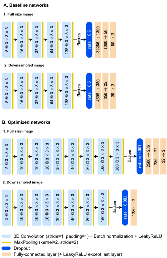
Figure 8: Diagrams of the network architectures used for classification. The first baseline architecture (A1) is the one used in [103], the second one (A2) is a very similar one adapted to process smaller inputs. The optimized architectures (B1) and (B2) are obtained independently with two different random searches. For convolution layers we specify the number of channels @ the kernel size and for the fully-connected layers we specify the number of input nodes $\rightarrow$ the number of output nodes. Each fully-connected layer is followed by a LeakyReLU activation except for the last one. For the dropout layer, the dropout rate is specified.

Appendix E A Few More Sampling Comparisons (Sec. 3.3)

In addition to the comparison performed in Sec. 3.3.1, we also compare qualitatively a Vanilla VAE, a VAE with VAMP prior and a geometry-aware VAE on four reduced data sets and in higher dimensional latent spaces of dimension 10. The first one is created with 180 binary rings and disks with different diameters and thicknesses ensuring balanced classes. The second one is composed of 120 samples of EMNIST (letter M) and referred to as reduced EMNIST. Another one is created with 120 samples from the classes 0, 1 and 2 of MNIST database ensuring balanced classes and is called reduced MNIST. The last one, reduced Fashion, is again composed of 120 samples from three classes (shoes, trouser and bag) from FashionMNIST and ensuring balanced classes. The models have the same architectures as described in Table VIII and are trained with the parameters stated in Table. XIII. Each model is trained until the ELBO does not improve for 20 epochs with Adam optimizer, a learning rate of $10^{-3}$ and in a single batch. In Fig. 10 are presented from top to bottom: 1) an extract of the training samples for each data set; 2) samples obtained with a vanilla VAE with a Gaussian prior; 2) data generated from a VAE with VAMP prior; 3) samples created by a geometry-aware VAE and using the prior or 4) samples from our method. As discussed in the paper, the proposed method is again able to visually outperform peers since for all data sets it is able to create sharper and more meaningful samples even if the number of training samples is quite small.

TABLE XIII: Geometry-aware VAE parameters.

Data sets	Parameters
	$d^{*}$	$K$	$\varepsilon$	$T$	$\lambda$	$\sqrt{\beta_{0}}$
Synthetic shapes	10	3	$10^{-2}$	1.5	$10^{-3}$	0.3
reduced MNIST	10	3	$10^{-2}$	1.5	$10^{-3}$	0.3
reduced EMNIST	10	3	$10^{-2}$	1.5	$10^{-3}$	0.3
reduced Fashion	10	3	$10^{-2}$	1.5	$10^{-3}$	0.3
* Latent space dimension (same for VAE and VAMP-VAE)

Appendix F Additional Results (Sec.4.2.3)

Further to the experiments presented in Sec. 4.2.3, we also provide the results of the four classifiers on reduced EMNIST and reduced Fashion in Fig. 9. Again, for most classifiers the proposed method either equals or greatly outperform the baseline.

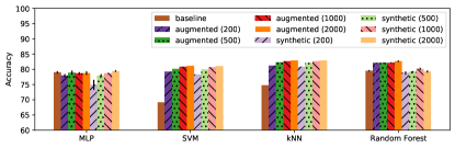
(a) reduced EMNIST

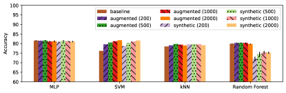
(b) reduced FashionMNIST

Figure 9: Evolution of the accuracy of four benchmark classifiers on the reduced EMNIST data set (top) and the reduced Fashion data set (bottom). Stochastic classifiers are trained with five independent runs and we report the mean accuracy and standard deviation on the test set.

Appendix G A few More Sample Generation on ADNI

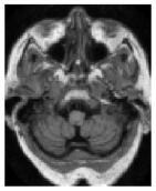
(a)

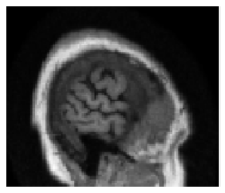
(b)

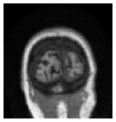
(c)

(d)

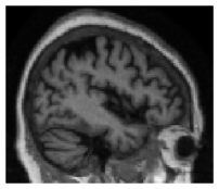
(e)

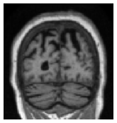
(f)

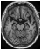
(g)

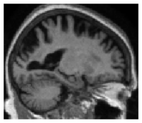
(h)

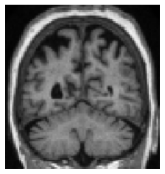
(i)

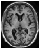
(j)

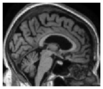
(k)

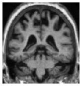
(l)

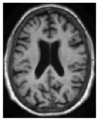
(m)

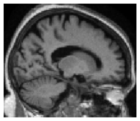
(n)

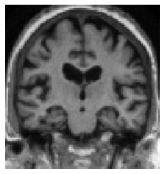
(o)

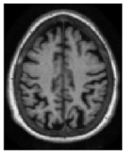
(p)

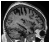
(q)

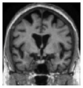
(r)

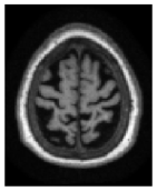
(s)

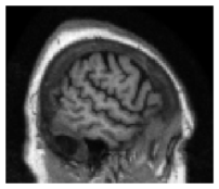
(t)

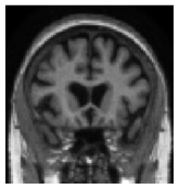
(u)

Figure 11: Several slices of a generated image. The model is trained on the AD class of train-50 (i.e. 50 images of AD patients).

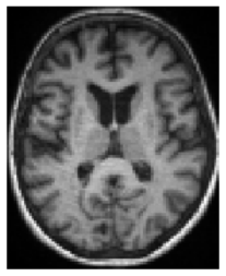
(a)

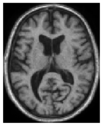
(b)

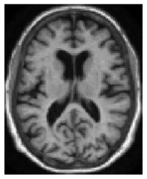
(c)

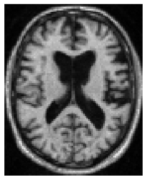
(d)

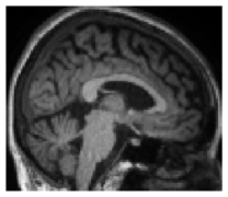
(e)

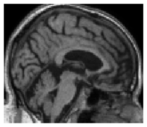
(f)

(g)

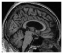
(h)

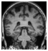
(i)

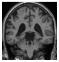
(j)

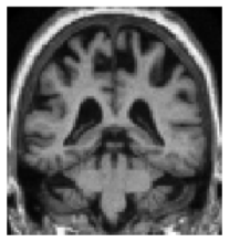
(k)

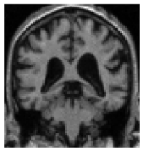
(l)

Figure 12: Images generated by our method when trained on train-50. Left: CN generated patients. Right: AD generated patients.

In this section, we first provide several slices of a 3D image generated by our model. The model is trained on the class AD of train-50 (i.e. on 50 MRI of patient having been diagnosed with Alzheimer’s disease). The generated image is presented in Fig. 11. We also present in Fig. 12, four generated patients for a model trained on train-50. The two left images show cognitively normal generated patients while the rightmost images represent AD generated patients.

Appendix H The Intruders: Answers to Fig. 7

In Fig. 7 of the paper, the synthetic samples are the leftmost and rightmost images while the real patients are in the middle. The model is trained on the class AD of train-full i.e. 210 images.

Appendix I Complementary Results on Medical Images

The comprehensive results for the classification task on MRIs are added in Tables XIV to XVII. As observed on the toy examples, the proposed model is again able to produce meaningful synthetic samples since each CNN outperforms greatly the baseline (i.e. the real training data) either on train-50 or train-full. The fact that classification performances on AIBL (which is never used for training) are better for a classifier trained on synthetic data than on the baseline shows again that the generative model does not overfit the training data (coming from ADNI) but rather produces samples that are also relevant for another database. Moreover, we again see that the classifier is able to outperform the baseline with only synthetic samples proof of good generalization power.

Training
samples       VAE +
$\mathcal{N}(0,I_{d})$       VAE +
VAMP prior       RHVAE +
$\mathcal{N}(0,I_{d})$       RHVAE +
Ours

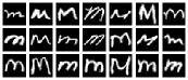
(a) reduced EMNIST (120)

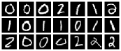
(b) reduced MNIST (120)

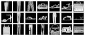
(c) reduced Fashion (120)

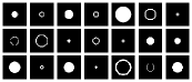
(d) Synthetic (180)

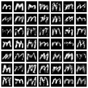
(e)

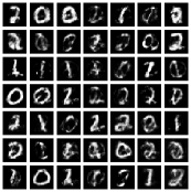
(f)

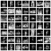
(g)

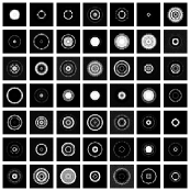
(h)

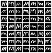
(i)

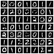
(j)

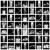
(k)

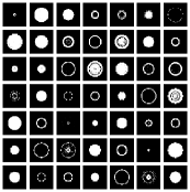
(l)

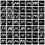
(m)

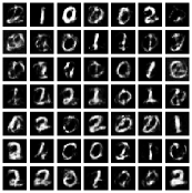
(n)

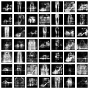
(o)

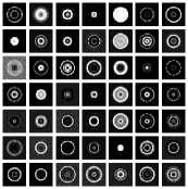
(p)

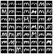
(q)

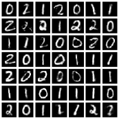
(r)

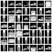
(s)

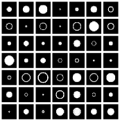
(t)

Figure 10: Comparison of four sampling methods on reduced EMNIST (120 letters M), reduced MNIST, reduced FashionMNIST and the synthetic data sets in higher dimensional latent spaces (dimension 10). From top to bottom: 1) samples extracted from the training set; 2) samples generated with a Vanilla VAE and using the prior ($\mathcal{N}(0,I_{d}$)); 3) from the VAMP prior VAE ; 4) from a RHVAE and the prior-based generation scheme and 5) from a RHVAE and using the proposed method. All the models are trained with the same encoder and decoder networks and identical latent space dimension. An early stopping strategy is adopted and consists in stopping training if the ELBO does not improve for 20 epochs. The number of training samples is noted between parenthesis.

TABLE XIV: Mean test performance of the 20 runs trained on train-50 with the baseline hyperparameters

		ADNI			AIBL
image type	synthetic	sensitivity	specificity	balanced	sensitivity	specificity	balanced
	images			accuracy			accuracy
real	-	$70.3\pm 12.2$	$62.4\pm 11.5$	$66.3\pm 2.4$	$60.7\pm 13.7$	$73.8\pm 7.2$	$67.2\pm 4.1$
real (high-resolution)	-	$78.5\pm 9.4$	$57.4\pm 8.8$	$67.9\pm 2.3$	$57.2\pm 11.2$	$75.8\pm 7.0$	$66.5\pm 3.0$
synthetic	500	$72.4\pm 6.4$	$65.6\pm 8.1$	$69.0\pm 1.9$	$56.6\pm 9.9$	$80.0\pm 5.3$	$68.3\pm 3.0$
synthetic	1000	$75.0\pm 6.2$	$65.6\pm 7.4$	$70.3\pm 2.0$	$62.7\pm 9.7$	$78.8\pm 5.3$	$70.8\pm 3.5$
synthetic	2000	$71.4\pm 6.6$	$70.4\pm 6.6$	$70.9\pm 3.0$	$62.1\pm 8.8$	$80.5\pm 4.7$	$71.3\pm 3.6$
synthetic	3000	$70.6\pm 5.2$	$\boldsymbol{73.8\pm 4.2}$	$72.2\pm 1.4$	$65.7\pm 6.9$	$80.5\pm 4.6$	$73.1\pm 1.8$
synthetic	5000	$\boldsymbol{78.1\pm 6.1}$	$69.0\pm 6.9$	$73.5\pm 2.0$	$\boldsymbol{74.5\pm 7.8}$	$77.3\pm 5.4$	$\boldsymbol{76.5\pm 2.9}$
synthetic	10000	$75.2\pm 6.8$	$73.4\pm 4.8$	$\boldsymbol{74.3\pm 1.9}$	$73.6\pm 10.8$	$\boldsymbol{79.4\pm 6.0}$	$75.9\pm 2.5$
synthetic + real	500	$71.9\pm 5.3$	$67.0\pm 4.5$	$69.4\pm 1.6$	$55.9\pm 6.8$	$81.1\pm 3.1$	$68.5\pm 2.5$
synthetic + real	1000	$69.8\pm 6.6$	$71.2\pm 3.7$	$70.5\pm 2.1$	$59.1\pm 9.0$	$82.1\pm 3.7$	$70.6\pm 3.1$
synthetic + real	2000	$72.2\pm 4.4$	$70.3\pm 4.3$	$71.2\pm 1.6$	$66.6\pm 7.1$	$79.0\pm 4.1$	$72.8\pm 2.2$
synthetic + real	3000	$71.8\pm 4.9$	$73.4\pm 5.5$	$72.6\pm 1.6$	$66.1\pm 9.3$	$81.1\pm 5.0$	$73.6\pm 3.0$
synthetic + real	5000	$\boldsymbol{74.7\pm 5.3}$	$\boldsymbol{73.5\pm 4.8}$	$\boldsymbol{74.1\pm 2.2}$	$\boldsymbol{71.7\pm 10.0}$	$80.5\pm 4.4$	$\boldsymbol{76.1\pm 3.6}$
synthetic + real	10000	$74.7\pm 7.0$	$73.4\pm 6.1$	$74.0\pm 2.7$	$69.1\pm 9.9$	$\boldsymbol{80.7\pm 5.1}$	$74.9\pm 3.2$

TABLE XV: Mean test performance of the 20 runs trained on train-full with the baseline hyperparameters

		ADNI			AIBL
image type	synthetic	sensitivity	specificity	balanced	sensitivity	specificity	balanced
	images			accuracy			accuracy
real	-	$79.1\pm 6.2$	$76.3\pm 4.2$	$77.7\pm 2.5$	$70.6\pm 6.7$	$86.3\pm 3.6$	$78.4\pm 2.4$
real (high-resolution)	-	$84.5\pm 3.8$	$76.7\pm 4.0$	$80.6\pm 1.1$	$71.6\pm 6.4$	$89.2\pm 2.7$	$80.4\pm 2.6$
synthetic	500	$81.6\pm 6.8$	$79.5\pm 5.8$	$80.5\pm 2.4$	$74.7\pm 9.3$	$87.3\pm 4.8$	$81.0\pm 3.2$
synthetic	1000	$82.9\pm 4.5$	$82.0\pm 5.8$	$82.4\pm 1.9$	$77.2\pm 7.4$	$88.8\pm 5.2$	$83.0\pm 2.0$
synthetic	2000	$81.9\pm 4.5$	$87.7\pm 3.4$	$84.8\pm 2.0$	$74.7\pm 6.3$	$92.1\pm 1.9$	$83.4\pm 2.7$
synthetic	3000	$\boldsymbol{84.9\pm 3.5}$	$87.4\pm 3.5$	$86.1\pm 1.5$	$77.4\pm 5.8$	$90.9\pm 3.0$	$84.2\pm 1.8$
synthetic	5000	$84.0\pm 3.5$	$88.4\pm 3.3$	$86.2\pm 1.7$	$76.8\pm 4.2$	$\boldsymbol{92.2\pm 1.8}$	$\boldsymbol{84.5\pm 1.8}$
synthetic	10000	$84.2\pm 5.4$	$\boldsymbol{88.6\pm 3.9}$	$\boldsymbol{86.4\pm 1.8}$	$\boldsymbol{77.5\pm 7.4}$	$91.0\pm 3.2$	$84.2\pm 2.4$
synthetic + real	500	$82.5\pm 3.4$	$81.9\pm 5.4$	$82.2\pm 2.4$	$76.0\pm 6.3$	$89.7\pm 3.3$	$82.9\pm 2.5$
synthetic + real	1000	$84.6\pm 4.4$	$84.3\pm 5.1$	$84.4\pm 1.8$	$77.0\pm 7.0$	$90.4\pm 3.4$	$83.7\pm 2.3$
synthetic + real	2000	$\boldsymbol{85.4\pm 4.0}$	$86.4\pm 5.9$	$85.9\pm 1.6$	$77.2\pm 6.9$	$90.4\pm 3.8$	$83.8\pm 2.2$
synthetic + real	3000	$84.7\pm 3.6$	$86.8\pm 4.5$	$85.8\pm 1.7$	$77.2\pm 4.8$	$\boldsymbol{91.7\pm 2.9}$	$84.4\pm 1.8$
synthetic + real	5000	$84.6\pm 4.2$	$86.9\pm 3.6$	$85.7\pm 2.1$	$76.9\pm 5.2$	$91.4\pm 3.0$	$84.2\pm 2.2$
synthetic + real	10000	$84.2\pm 2.8$	$\boldsymbol{88.5\pm 2.9}$	$\boldsymbol{86.3\pm 1.8}$	$\boldsymbol{79.1\pm 4.7}$	$91.0\pm 2.6$	$\boldsymbol{85.1\pm 1.9}$

TABLE XVI: Mean test performance of the 20 runs trained on train-50 with the optimized hyperparameters

		ADNI			AIBL
image type	synthetic	sensitivity	specificity	balanced	sensitivity	specificity	balanced
	images			accuracy			accuracy
real	-	$75.4\pm 5.0$	$75.5\pm 5.3$	$75.5\pm 2.7$	$68.6\pm 8.5$	$82.6\pm 4.2$	$75.6\pm 4.1$
real (high-resolution)	-	$73.6\pm 6.2$	$70.6\pm 5.9$	$72.1\pm 3.1$	$57.8\pm 12.3$	$84.6\pm 4.2$	$71.2\pm 5.1$
synthetic	500	$75.8\pm 3.0$	$77.6\pm 5.3$	$76.7\pm 2.8$	$73.2\pm 9.0$	$\boldsymbol{83.6\pm 4.0}$	$78.4\pm 4.0$
synthetic	1000	$76.7\pm 4.6$	$78.5\pm 4.9$	$\boldsymbol{77.6\pm 3.7}$	$78.7\pm 7.5$	$83.2\pm 4.8$	$80.9\pm 4.3$
synthetic	2000	$73.9\pm 3.6$	$\boldsymbol{79.8\pm 4.0}$	$76.8\pm 3.0$	$78.2\pm 6.9$	$82.4\pm 3.7$	$80.3\pm 3.5$
synthetic	3000	$74.4\pm 6.1$	$79.8\pm 4.9$	$77.1\pm 4.0$	$76.4\pm 10.1$	$82.4\pm 4.3$	$79.4\pm 4.7$
synthetic	5000	$77.1\pm 4.5$	$77.4\pm 5.2$	$77.2\pm 2.1$	$81.1\pm 5.9$	$82.0\pm 3.9$	$\boldsymbol{81.5\pm 2.6}$
synthetic	10000	$\boldsymbol{77.5\pm 5.3}$	$77.3\pm 4.7$	$77.4\pm 3.1$	$\boldsymbol{81.7\pm 5.4}$	$79.7\pm 4.1$	$80.7\pm 2.9$
synthetic + real	500	$73.2\pm 4.2$	$78.0\pm 3.3$	$75.6\pm 2.5$	$69.2\pm 9.4$	$\boldsymbol{82.7\pm 4.1}$	$76.0\pm 4.2$
synthetic + real	1000	$76.1\pm 5.3$	$\boldsymbol{79.5\pm 2.9}$	$77.8\pm 2.3$	$79.3\pm 5.8$	$82.5\pm 4.2$	$80.9\pm 3.2$
synthetic + real	2000	$75.2\pm 3.8$	$78.6\pm 4.4$	$76.9\pm 2.4$	$77.8\pm 8.8$	$82.2\pm 4.5$	$80.0\pm 3.6$
synthetic + real	3000	$76.5\pm 3.8$	$79.2\pm 4.2$	$77.8\pm 1.9$	$80.9\pm 7.9$	$81.4\pm 4.2$	$81.2\pm 3.7$
synthetic + real	5000	$77.1\pm 3.7$	$76.7\pm 4.1$	$76.9\pm 2.5$	$80.7\pm 6.1$	$81.2\pm 3.7$	$80.9\pm 2.7$
synthetic + real	10000	$\boldsymbol{77.8\pm 4.6}$	$78.2\pm 4.9$	$\boldsymbol{78.0\pm 2.1}$	$\boldsymbol{81.7\pm 4.9}$	$81.9\pm 4.6$	$\boldsymbol{81.9\pm 2.2}$

TABLE XVII: Mean test performance of the 20 runs trained on train-full with the optimized hyperparameters

		ADNI			AIBL
image type	synthetic	sensitivity	specificity	balanced	sensitivity	specificity	balanced
	images			accuracy			accuracy
real	-	$82.5\pm 4.2$	$88.5\pm 6.6$	$85.5\pm 2.4$	$75.1\pm 8.4$	$88.7\pm 9.0$	$81.9\pm 3.2$
real (high-resolution)	-	$82.6\pm 4.5$	$88.9\pm 6.3$	$85.7\pm 2.5$	$78.9\pm 5.4$	$89.9\pm 4.0$	$84.4\pm 1.7$
synthetic	500	$81.7\pm 3.6$	$90.5\pm 3.9$	$86.1\pm 1.4$	$75.5\pm 7.1$	$89.8\pm 4.3$	$82.6\pm 2.9$
synthetic	1000	$82.8\pm 3.4$	$90.0\pm 4.0$	$86.4\pm 2.1$	$76.8\pm 4.5$	$91.5\pm 2.5$	$84.2\pm 1.7$
synthetic	2000	$81.3\pm 2.8$	$91.2\pm 2.8$	$86.2\pm 1.7$	$76.2\pm 6.7$	$\boldsymbol{92.2\pm 3.6}$	$84.2\pm 2.6$
synthetic	3000	$82.2\pm 4.9$	$90.6\pm 4.5$	$86.4\pm 2.0$	$77.7\pm 6.3$	$90.8\pm 4.4$	$84.3\pm 2.0$
synthetic	5000	$80.6\pm 3.4$	$\boldsymbol{91.6\pm 2.5}$	$86.1\pm 1.9$	$75.3\pm 5.4$	$92.4\pm 2.5$	$83.8\pm 2.0$
synthetic	10000	$\boldsymbol{84.0\pm 3.8}$	$89.1\pm 3.1$	$\boldsymbol{86.5\pm 1.7}$	$\boldsymbol{79.2\pm 5.2}$	$90.1\pm 3.7$	$\boldsymbol{84.7\pm 2.3}$
synthetic + real	500	$82.3\pm 2.3$	$89.8\pm 2.7$	$86.0\pm 1.8$	$74.9\pm 5.0$	$91.4\pm 2.6$	$83.2\pm 2.4$
synthetic + real	1000	$82.5\pm 3.3$	$90.5\pm 4.1$	$86.5\pm 1.9$	$76.4\pm 5.6$	$91.0\pm 3.4$	$83.7\pm 2.0$
synthetic + real	2000	$\boldsymbol{83.1\pm 4.2}$	$\boldsymbol{91.3\pm 3.2}$	$\boldsymbol{87.2\pm 1.7}$	$76.0\pm 4.7$	$92.0\pm 2.4$	$84.0\pm 2.0$
synthetic + real	3000	$81.3\pm 3.7$	$90.4\pm 3.4$	$85.8\pm 2.6$	$74.9\pm 7.3$	$92.3\pm 2.6$	$83.6\pm 3.2$
synthetic + real	5000	$81.9\pm 3.5$	$90.9\pm 2.5$	$86.4\pm 1.3$	$74.1\pm 4.9$	$\boldsymbol{92.9\pm 1.9}$	$83.5\pm 2.2$
synthetic + real	10000	$82.2\pm 3.4$	$91.2\pm 3.6$	$86.7\pm 1.8$	$\boldsymbol{76.4\pm 4.2}$	$92.1\pm 2.1$	$\boldsymbol{84.3\pm 1.8}$

References

- [1] K. S. Button, J. P. Ioannidis, C. Mokrysz, B. A. Nosek, J. Flint, E. S. Robinson, and M. R. Munafò, “Power failure: why small sample size undermines the reliability of neuroscience,” Nature Reviews Neuroscience, vol. 14, no. 5, pp. 365–376, 2013.
- [2] B. O. Turner, E. J. Paul, M. B. Miller, and A. K. Barbey, “Small sample sizes reduce the replicability of task-based fMRI studies,” Communications Biology, vol. 1, no. 1, pp. 1–10, 2018.
- [3] I. Goodfellow, Y. Bengio, A. Courville, and Y. Bengio, Deep learning. MIT press Cambridge, 2016, vol. 1, issue: 2.
- [4] C. Shorten and T. M. Khoshgoftaar, “A survey on Image Data Augmentation for Deep Learning,” Journal of Big Data, vol. 6, no. 1, p. 60, 2019.
- [5] M. A. Tanner and W. H. Wong, “The calculation of posterior distributions by data augmentation,” Journal of the American statistical Association, vol. 82, no. 398, pp. 528–540, 1987.
- [6] N. V. Chawla, K. W. Bowyer, L. O. Hall, and W. P. Kegelmeyer, “SMOTE: synthetic minority over-sampling technique,” Journal of artificial intelligence research, vol. 16, pp. 321–357, 2002.
- [7] H. Han, W.-Y. Wang, and B.-H. Mao, “Borderline-SMOTE: A new over-sampling method in imbalanced data sets learning,” in Advances in Intelligent Computing, D.-S. Huang, X.-P. Zhang, and G.-B. Huang, Eds. Springer Berlin Heidelberg, 2005, vol. 3644, pp. 878–887, series Title: LNCS.
- [8] H. M. Nguyen, E. W. Cooper, and K. Kamei, “Borderline over-sampling for imbalanced data classification,” International Journal of Knowledge Engineering and Soft Data Paradigms, vol. 3, no. 1, pp. 4–21, 2011.
- [9] Haibo He, Yang Bai, E. A. Garcia, and Shutao Li, “ADASYN: Adaptive synthetic sampling approach for imbalanced learning,” in 2008 IEEE International Joint Conference on Neural Networks (IEEE World Congress on Computational Intelligence). IEEE, 2008, pp. 1322–1328.
- [10] S. Barua, M. M. Islam, X. Yao, and K. Murase, “MWMOTE–majority weighted minority oversampling technique for imbalanced data set learning,” IEEE Transactions on Knowledge and Data Engineering, vol. 26, no. 2, pp. 405–425, 2012.
- [11] R. Blagus and L. Lusa, “SMOTE for high-dimensional class-imbalanced data,” BMC Bioinformatics, vol. 14, no. 1, p. 106, 2013.
- [12] A. Fernández, S. Garcia, F. Herrera, and N. V. Chawla, “SMOTE for learning from imbalanced data: progress and challenges, marking the 15-year anniversary,” Journal of artificial intelligence research, vol. 61, pp. 863–905, 2018.
- [13] I. Goodfellow, J. Pouget-Abadie, M. Mirza, B. Xu, D. Warde-Farley, S. Ozair, A. Courville, and Y. Bengio, “Generative adversarial nets,” in Advances in Neural Information Processing Systems, 2014, pp. 2672–2680.
- [14] D. P. Kingma and M. Welling, “Auto-encoding variational bayes,” arXiv:1312.6114 [cs, stat], 2014.
- [15] D. J. Rezende, S. Mohamed, and D. Wierstra, “Stochastic backpropagation and approximate inference in deep generative models,” in International conference on machine learning. PMLR, 2014, pp. 1278–1286.
- [16] X. Zhu, Y. Liu, J. Li, T. Wan, and Z. Qin, “Emotion classification with data augmentation using generative adversarial networks,” in Pacific-Asia conference on knowledge discovery and data mining. Springer, 2018, pp. 349–360.
- [17] G. Mariani, F. Scheidegger, R. Istrate, C. Bekas, and C. Malossi, “BAGAN: Data Augmentation with Balancing GAN,” arXiv:1803.09655, 2018.
- [18] A. Antoniou, A. Storkey, and H. Edwards, “Data augmentation generative adversarial networks,” arXiv:1711.04340 [cs, stat], 2018-03-21.
- [19] S. K. Lim, Y. Loo, N.-T. Tran, N.-M. Cheung, G. Roig, and Y. Elovici, “Doping: Generative data augmentation for unsupervised anomaly detection with gan,” in 2018 IEEE International Conference on Data Mining (ICDM). IEEE, 2018, pp. 1122–1127.
- [20] Y. Zhu, M. Aoun, M. Krijn, J. Vanschoren, and H. T. Campus, “Data Augmentation using Conditional Generative Adversarial Networks for Leaf Counting in Arabidopsis Plants.” in BMVC, 2018, p. 324.
- [21] X. Yi, E. Walia, and P. Babyn, “Generative adversarial network in medical imaging: A review,” Medical image analysis, vol. 58, p. 101552, 2019.
- [22] H.-C. Shin, N. A. Tenenholtz, J. K. Rogers, C. G. Schwarz, M. L. Senjem, J. L. Gunter, K. P. Andriole, and M. Michalski, “Medical image synthesis for data augmentation and anonymization using generative adversarial networks,” in International Workshop on Simulation and Synthesis in Medical Imaging, ser. LNCS. Springer, 2018, pp. 1–11.
- [23] F. Calimeri, A. Marzullo, C. Stamile, and G. Terracina, “Biomedical data augmentation using generative adversarial neural networks,” in International conference on artificial neural networks. Springer, 2017, pp. 626–634.
- [24] M. Frid-Adar, I. Diamant, E. Klang, M. Amitai, J. Goldberger, and H. Greenspan, “GAN-based synthetic medical image augmentation for increased CNN performance in liver lesion classification,” Neurocomputing, vol. 321, pp. 321–331, 2018.
- [25] V. Sandfort, K. Yan, P. J. Pickhardt, and R. M. Summers, “Data augmentation using generative adversarial networks (CycleGAN) to improve generalizability in CT segmentation tasks,” Scientific reports, vol. 9, no. 1, p. 16884, 2019.
- [26] A. Madani, M. Moradi, A. Karargyris, and T. Syeda-Mahmood, “Chest x-ray generation and data augmentation for cardiovascular abnormality classification,” in Medical Imaging 2018: Image Processing, vol. 10574. International Society for Optics and Photonics, 2018, p. 105741M.
- [27] H. Salehinejad, S. Valaee, T. Dowdell, E. Colak, and J. Barfett, “Generalization of deep neural networks for chest pathology classification in x-rays using generative adversarial networks,” in 2018 IEEE International Conference on Acoustics, Speech and Signal Processing (ICASSP). IEEE, 2018, pp. 990–994.
- [28] A. Waheed, M. Goyal, D. Gupta, A. Khanna, F. Al-Turjman, and P. R. Pinheiro, “Covidgan: data augmentation using auxiliary classifier gan for improved covid-19 detection,” Ieee Access, vol. 8, pp. 91 916–91 923, 2020.
- [29] L. Bi, J. Kim, A. Kumar, D. Feng, and M. Fulham, “Synthesis of Positron Emission Tomography (PET) Images via Multi-channel Generative Adversarial Networks (GANs),” in Molecular Imaging, Reconstruction and Analysis of Moving Body Organs, and Stroke Imaging and Treatment, ser. LNCS. Springer, 2017, pp. 43–51.
- [30] Y. Liu, Y. Zhou, X. Liu, F. Dong, C. Wang, and Z. Wang, “Wasserstein gan-based small-sample augmentation for new-generation artificial intelligence: a case study of cancer-staging data in biology,” Engineering, vol. 5, no. 1, pp. 156–163, 2019.
- [31] C. Baur, S. Albarqouni, and N. Navab, “Generating highly realistic images of skin lesions with GANs,” in OR 2.0 Context-Aware Operating Theaters, Computer Assisted Robotic Endoscopy, Clinical Image-Based Procedures, and Skin Image Analysis. Springer, 2018, pp. 260–267.
- [32] D. Korkinof, T. Rijken, M. O’Neill, J. Yearsley, H. Harvey, and B. Glocker, “High-resolution mammogram synthesis using progressive generative adversarial networks,” arXiv preprint arXiv:1807.03401, 2018.
- [33] E. Wu, K. Wu, D. Cox, and W. Lotter, “Conditional infilling gans for data augmentation in mammogram classification,” in Image analysis for moving organ, breast, and thoracic images. Springer, 2018, pp. 98–106.
- [34] W.-N. Hsu, Y. Zhang, and J. Glass, “Unsupervised domain adaptation for robust speech recognition via variational autoencoder-based data augmentation,” in 2017 IEEE Automatic Speech Recognition and Understanding Workshop (ASRU). IEEE, 2017, pp. 16–23.
- [35] H. Nishizaki, “Data augmentation and feature extraction using variational autoencoder for acoustic modeling,” in 2017 Asia-Pacific Signal and Information Processing Association Annual Summit and Conference (APSIPA ASC). IEEE, 2017, pp. 1222–1227.
- [36] Z. Wu, S. Wang, Y. Qian, and K. Yu, “Data augmentation using variational autoencoder for embedding based speaker verification,” in Interspeech 2019. ISCA, 2019, pp. 1163–1167.
- [37] P. Zhuang, A. G. Schwing, and O. Koyejo, “fMRI data augmentation via synthesis,” in 2019 IEEE 16th International Symposium on Biomedical Imaging (ISBI 2019). IEEE, 2019, pp. 1783–1787.
- [38] X. Liu, Y. Zou, L. Kong, Z. Diao, J. Yan, J. Wang, S. Li, P. Jia, and J. You, “Data augmentation via latent space interpolation for image classification,” in 2018 24th International Conference on Pattern Recognition (ICPR). IEEE, 2018, pp. 728–733.
- [39] N. Painchaud, Y. Skandarani, T. Judge, O. Bernard, A. Lalande, and P.-M. Jodoin, “Cardiac MRI segmentation with strong anatomical guarantees,” in International Conference on Medical Image Computing and Computer-Assisted Intervention. Springer, 2019, pp. 632–640.
- [40] R. Selvan, E. B. Dam, N. S. Detlefsen, S. Rischel, K. Sheng, M. Nielsen, and A. Pai, “Lung segmentation from chest x-rays using variational data imputation,” arXiv:2005.10052 [cs, eess, stat], 2020.
- [41] A. Myronenko, “3D MRI brain tumor segmentation using autoencoder regularization,” in International MICCAI Brainlesion Workshop. Springer, 2018, pp. 311–320.
- [42] M. I. Jordan, Z. Ghahramani, T. S. Jaakkola, and L. K. Saul, “An introduction to variational methods for graphical models,” Machine Learning, vol. 37, no. 2, pp. 183–233, 1999.
- [43] Y. Burda, R. Grosse, and R. Salakhutdinov, “Importance weighted autoencoders,” arXiv:1509.00519 [cs, stat], 2016-11-07.
- [44] A. A. Alemi, I. Fischer, J. V. Dillon, and K. Murphy, “Deep variational information bottleneck,” arXiv preprint arXiv:1612.00410, 2016.
- [45] I. Higgins, L. Matthey, A. Pal, C. Burgess, X. Glorot, M. Botvinick, S. Mohamed, and A. Lerchner, “beta-VAE: Learning basic visual concepts with a constrained variational framework.” ICLR, vol. 2, no. 5, p. 6, 2017.
- [46] C. Cremer, X. Li, and D. Duvenaud, “Inference suboptimality in variational autoencoders,” in International Conference on Machine Learning. PMLR, 2018, pp. 1078–1086.
- [47] C. Zhang, J. Bütepage, H. Kjellström, and S. Mandt, “Advances in variational inference,” IEEE Transactions on Pattern Analysis and Machine Intelligence, vol. 41, no. 8, pp. 2008–2026, 2018.
- [48] F. Ruiz and M. Titsias, “A contrastive divergence for combining variational inference and mcmc,” in International Conference on Machine Learning. PMLR, 2019, pp. 5537–5545.
- [49] T. Salimans, D. Kingma, and M. Welling, “Markov chain monte carlo and variational inference: Bridging the gap,” in International Conference on Machine Learning, 2015, pp. 1218–1226.
- [50] D. Rezende and S. Mohamed, “Variational inference with normalizing flows,” in International Conference on Machine Learning. PMLR, 2015, pp. 1530–1538.
- [51] R. M. Neal and others, “MCMC using hamiltonian dynamics,” Handbook of Markov Chain Monte Carlo, vol. 2, no. 11, p. 2, 2011.
- [52] A. L. Caterini, A. Doucet, and D. Sejdinovic, “Hamiltonian variational auto-encoder,” in Advances in Neural Information Processing Systems, 2018, pp. 8167–8177.
- [53] M. D. Hoffman and M. J. Johnson, “Elbo surgery: yet another way to carve up the variational evidence lower bound,” in Workshop in Advances in Approximate Bayesian Inference, NIPS, vol. 1, 2016, p. 2.
- [54] E. Nalisnick, L. Hertel, and P. Smyth, “Approximate inference for deep latent gaussian mixtures,” in NIPS Workshop on Bayesian Deep Learning, vol. 2, 2016, p. 131.
- [55] N. Dilokthanakul, P. A. M. Mediano, M. Garnelo, M. C. H. Lee, H. Salimbeni, K. Arulkumaran, and M. Shanahan, “Deep unsupervised clustering with gaussian mixture variational autoencoders,” arXiv:1611.02648 [cs, stat], 2017.
- [56] J. Tomczak and M. Welling, “Vae with a vampprior,” in International Conference on Artificial Intelligence and Statistics. PMLR, 2018, pp. 1214–1223.
- [57] C. K. Sønderby, T. Raiko, L. Maaløe, S. K. Sønderby, and O. Winther, “Ladder variational autoencoder,” in 29th Annual Conference on Neural Information Processing Systems (NIPS 2016), 2016.
- [58] A. Klushyn, N. Chen, R. Kurle, and B. Cseke, “Learning Hierarchical Priors in VAEs,” Advances in neural information processing systems, p. 10, 2019.
- [59] X. Chen, D. P. Kingma, T. Salimans, Y. Duan, P. Dhariwal, J. Schulman, I. Sutskever, and P. Abbeel, “Variational lossy autoencoder,” arXiv preprint arXiv:1611.02731, 2016.
- [60] A. Razavi, A. v. d. Oord, and O. Vinyals, “Generating diverse high-fidelity images with vq-vae-2,” Advances in Neural Information Processing Systems, 2020.
- [61] B. Pang, T. Han, E. Nijkamp, S.-C. Zhu, and Y. N. Wu, “Learning latent space energy-based prior model,” Advances in Neural Information Processing Systems, vol. 33, 2020.
- [62] J. Aneja, A. Schwing, J. Kautz, and A. Vahdat, “NCP-VAE: Variational autoencoders with noise contrastive priors,” arXiv:2010.02917 [cs, stat], 2020.
- [63] P. Ghosh, M. S. Sajjadi, A. Vergari, M. Black, and B. Schölkopf, “From variational to deterministic autoencoders,” in 8th International Conference on Learning Representations, ICLR 2020, 2020.
- [64] M. Bauer and A. Mnih, “Resampled priors for variational autoencoders,” in The 22nd International Conference on Artificial Intelligence and Statistics. PMLR, 2019, pp. 66–75.
- [65] T. R. Davidson, L. Falorsi, N. De Cao, T. Kipf, and J. M. Tomczak, “Hyperspherical variational auto-encoders,” in 34th Conference on Uncertainty in Artificial Intelligence 2018, UAI 2018. Association For Uncertainty in Artificial Intelligence (AUAI), 2018, pp. 856–865.
- [66] E. Mathieu, C. Le Lan, C. J. Maddison, R. Tomioka, and Y. W. Teh, “Continuous hierarchical representations with poincaré variational auto-encoders,” in Advances in neural information processing systems, 2019, pp. 12 565–12 576.
- [67] I. Ovinnikov, “Poincaré wasserstein autoencoder,” arXiv:1901.01427 [cs, stat], 2020-03-16.
- [68] L. Falorsi, P. de Haan, T. R. Davidson, N. De Cao, M. Weiler, P. Forré, and T. S. Cohen, “Explorations in homeomorphic variational auto-encoding,” arXiv:1807.04689 [cs, stat], 2018.
- [69] N. Miolane and S. Holmes, “Learning weighted submanifolds with variational autoencoders and riemannian variational autoencoders,” in Proceedings of the IEEE/CVF Conference on Computer Vision and Pattern Recognition, 2020, pp. 14 503–14 511.
- [70] G. Arvanitidis, L. K. Hansen, and S. Hauberg, “A locally adaptive normal distribution,” Advances in Neural Information Processing Systems, pp. 4258–4266, 2016.
- [71] N. Chen, A. Klushyn, R. Kurle, X. Jiang, J. Bayer, and P. Smagt, “Metrics for deep generative models,” in International Conference on Artificial Intelligence and Statistics. PMLR, 2018, pp. 1540–1550.
- [72] H. Shao, A. Kumar, and P. T. Fletcher, “The riemannian geometry of deep generative models,” in 2018 IEEE/CVF Conference on Computer Vision and Pattern Recognition Workshops (CVPRW). IEEE, 2018, pp. 428–4288.
- [73] D. Kalatzis, D. Eklund, G. Arvanitidis, and S. Hauberg, “Variational autoencoders with riemannian brownian motion priors,” in International Conference on Machine Learning. PMLR, 2020, pp. 5053–5066.
- [74] M. Girolami and B. Calderhead, “Riemann manifold langevin and hamiltonian monte carlo methods,” Journal of the Royal Statistical Society: Series B (Statistical Methodology), vol. 73, no. 2, pp. 123–214, 2011.
- [75] S. Duane, A. D. Kennedy, B. J. Pendleton, and D. Roweth, “Hybrid monte carlo,” Physics Letters B, vol. 195, no. 2, pp. 216–222, 1987.
- [76] B. Leimkuhler and S. Reich, Simulating hamiltonian dynamics. Cambridge university press, 2004, vol. 14.
- [77] E. Hairer, C. Lubich, and G. Wanner, Geometric numerical integration: structure-preserving algorithms for ordinary differential equations. Springer Science & Business Media, 2006, vol. 31.
- [78] J. S. Liu, Monte Carlo strategies in scientific computing. Springer Science & Business Media, 2008.
- [79] A. Paszke, S. Gross, S. Chintala, G. Chanan, E. Yang, Z. DeVito, Z. Lin, A. Desmaison, L. Antiga, and A. Lerer, “Automatic differentiation in pytorch,” 2017.
- [80] G. Arvanitidis, L. K. Hansen, and S. Hauberg, “Latent space oddity: On the curvature of deep generative models,” in 6th International Conference on Learning Representations, ICLR 2018, 2018.
- [81] M. F. Frenzel, B. Teleaga, and A. Ushio, “Latent space cartography: Generalised metric-inspired measures and measure-based transformations for generative models,” arXiv preprint arXiv:1902.02113, 2019.
- [82] G. Arvanitidis, S. Hauberg, and B. Schölkopf, “Geometrically enriched latent spaces,” arXiv:2008.00565 [cs, stat], 2020-08-02.
- [83] G. Lebanon, “Metric learning for text documents,” IEEE Transactions on Pattern Analysis and Machine Intelligence, vol. 28, no. 4, pp. 497–508, 2006.
- [84] M. Louis, “Computational and statistical methods for trajectory analysis in a Riemannian geometry setting,” PhD Thesis, Sorbonnes universités, 2019.
- [85] B. Dai and D. Wipf, “Diagnosing and enhancing vae models,” in International Conference on Learning Representations, 2018.
- [86] R. M. Neal, “Hamiltonian importance sampling,” in talk presented at the Banff International Research Station (BIRS) workshop on Mathematical Issues in Molecular Dynamics, 2005.
- [87] H. Xiao, K. Rasul, and R. Vollgraf, “Fashion-mnist: a novel image dataset for benchmarking machine learning algorithms,” arXiv preprint arXiv:1708.07747, 2017.
- [88] G. Cohen, S. Afshar, J. Tapson, and A. Van Schaik, “Emnist: Extending mnist to handwritten letters,” in 2017 International Joint Conference on Neural Networks (IJCNN). IEEE, 2017, pp. 2921–2926.
- [89] Y. LeCun, “The MNIST database of handwritten digits,” 1998.
- [90] T. Salimans, I. Goodfellow, W. Zaremba, V. Cheung, A. Radford, and X. Chen, “Improved techniques for training gans,” in Advances in Neural Information Processing Systems, 2016.
- [91] M. Heusel, H. Ramsauer, T. Unterthiner, B. Nessler, and S. Hochreiter, “Gans trained by a two time-scale update rule converge to a local nash equilibrium,” in Advances in Neural Information Processing Systems, 2017.
- [92] T. Karras, T. Aila, S. Laine, and J. Lehtinen, “Progressive growing of gans for improved quality, stability, and variation,” in International Conference on Learning Representations (ICLR), 2017.
- [93] M. Lucic, K. Kurach, M. Michalski, S. Gelly, and O. Bousquet, “Are GANs created equal? a large-scale study,” in Advances in Neural Information Processing Systems, 2018, p. 10.
- [94] K. Shmelkov, C. Schmid, and K. Alahari, “How good is my gan?” in Proceedings of the European Conference on Computer Vision (ECCV), 2018, pp. 213–229.
- [95] A. Borji, “Pros and cons of GAN evaluation measures,” Computer Vision and Image Understanding, vol. 179, pp. 41–65, 2019.
- [96] B. Amos, “bamos/densenet.pytorch,” 2020, original-date: 2017-02-09T15:33:23Z. [Online]. Available: https://github.com/bamos/densenet.pytorch
- [97] G. Huang, Z. Liu, L. Van Der Maaten, and K. Q. Weinberger, “Densely connected convolutional networks,” in 2017 IEEE Conference on Computer Vision and Pattern Recognition (CVPR). IEEE, 2017, pp. 2261–2269.
- [98] A. Krizhevsky, G. Hinton et al., “Learning multiple layers of features from tiny images,” 2009.
- [99] L. Breiman, “Random forests,” Machine Learning, vol. 45, no. 1, pp. 5–32, 2001.
- [100] S. B. Kotsiantis, I. Zaharakis, and P. Pintelas, “Supervised machine learning: A review of classification techniques,” Emerging artificial intelligence applications in computer engineering, vol. 160, no. 1, pp. 3–24, 2007.
- [101] A. Routier, N. Burgos, M. Díaz, M. Bacci, S. Bottani, O. El-Rifai, S. Fontanella, P. Gori, J. Guillon, A. Guyot, R. Hassanaly, T. Jacquemont, P. Lu, A. Marcoux, T. Moreau, J. Samper-González, M. Teichmann, E. Thibeau-Sutre, G. Vaillant, J. Wen, A. Wild, M.-O. Habert, S. Durrleman, and O. Colliot, “Clinica: An Open-Source Software Platform for Reproducible Clinical Neuroscience Studies,” Frontiers in Neuroinformatics, vol. 15, p. 689675, 2021.
- [102] E. Thibeau-Sutre, M. Diaz, R. Hassanaly, A. M. Routier, D. Dormont, O. Colliot, and N. Burgos, “ClinicaDL: An open-source deep learning software for reproducible neuroimaging processing,” 2021.
- [103] J. Wen, E. Thibeau-Sutre, M. Diaz-Melo, J. Samper-González, A. Routier, S. Bottani, D. Dormont, S. Durrleman, N. Burgos, and O. Colliot, “Convolutional neural networks for classification of Alzheimer’s disease: Overview and reproducible evaluation,” Medical Image Analysis, vol. 63, p. 101694, 2020.
- [104] K. Aderghal, M. Boissenin, J. Benois-Pineau, G. Catheline, and K. Afdel, “Classification of sMRI for AD diagnosis with convolutional neuronal networks: A pilot 2-D+ study on ADNI,” in MultiMedia Modeling, vol. 10132 LNCS, 2017, pp. 690–701.
- [105] K. Aderghal, A. Khvostikov, A. Krylov, J. Benois-Pineau, K. Afdel, and G. Catheline, “Classification of Alzheimer Disease on Imaging Modalities with Deep CNNs Using Cross-Modal Transfer Learning,” in 2018 IEEE 31st International Symposium on Computer-Based Medical Systems (CBMS), 2018, pp. 345–350, iSSN: 2372-9198.
- [106] J. Islam and Y. Zhang, “GAN-based synthetic brain PET image generation,” Brain Informatics, vol. 7, no. 1, 2020.
- [107] K. Oh, Y.-C. Chung, K. W. Kim, W.-S. Kim, and I.-S. Oh, “Classification and Visualization of Alzheimer’s Disease using Volumetric Convolutional Neural Network and Transfer Learning,” Scientific Reports, vol. 9, no. 1, p. 18150, 2019.
- [108] M. Liu, J. Zhang, C. Lian, and D. Shen, “Weakly Supervised Deep Learning for Brain Disease Prognosis Using MRI and Incomplete Clinical Scores,” IEEE Transactions on Cybernetics, vol. 50, no. 7, pp. 3381–3392, 2020.
- [109] A. Valliani and A. Soni, “Deep Residual Nets for Improved Alzheimer’s Diagnosis,” in 8th ACM International Conference on Bioinformatics, Computational Biology,and Health Informatics - ACM-BCB ’17. Boston, Massachusetts, USA: ACM Press, 2017, pp. 615–615.
- [110] K. Bäckström, M. Nazari, I.-H. Gu, and A. Jakola, “An efficient 3D deep convolutional network for Alzheimer’s disease diagnosis using MR images,” in 2018 IEEE 15th International Symposium on Biomedical Imaging (ISBI 2018), vol. 2018-April, 2018, pp. 149–153.
- [111] D. Cheng and M. Liu, “CNNs based multi-modality classification for AD diagnosis,” in 2017 10th International Congress on Image and Signal Processing, BioMedical Engineering and Informatics (CISP-BMEI), 2017, pp. 1–5.
- [112] K. A. Ellis, A. I. Bush, D. Darby, D. De Fazio, J. Foster, P. Hudson, N. T. Lautenschlager, N. Lenzo, R. N. Martins, P. Maruff, C. Masters, A. Milner, K. Pike, C. Rowe, G. Savage, C. Szoeke, K. Taddei, V. Villemagne, M. Woodward, D. Ames, and AIBL Research Group, “The Australian Imaging, Biomarkers and Lifestyle (AIBL) study of aging: methodology and baseline characteristics of 1112 individuals recruited for a longitudinal study of Alzheimer’s disease,” International Psychogeriatrics, vol. 21, no. 4, pp. 672–687, 2009.
- [113] K. J. Gorgolewski, T. Auer, V. D. Calhoun, R. C. Craddock, S. Das, E. P. Duff, G. Flandin, S. S. Ghosh, T. Glatard, Y. O. Halchenko, D. A. Handwerker, M. Hanke, D. Keator, X. Li, Z. Michael, C. Maumet, B. N. Nichols, T. E. Nichols, J. Pellman, J.-B. Poline, A. Rokem, G. Schaefer, V. Sochat, W. Triplett, J. A. Turner, G. Varoquaux, and R. A. Poldrack, “The brain imaging data structure, a format for organizing and describing outputs of neuroimaging experiments,” Scientific Data, vol. 3, no. 1, p. 160044, 2016.
- [114] N. J. Tustison, B. B. Avants, P. A. Cook, Yuanjie Zheng, A. Egan, P. A. Yushkevich, and J. C. Gee, “N4ITK: Improved N3 Bias Correction,” IEEE Transactions on Medical Imaging, vol. 29, no. 6, pp. 1310–1320, 2010.
- [115] V. Fonov, A. Evans, R. McKinstry, C. Almli, and D. Collins, “Unbiased nonlinear average age-appropriate brain templates from birth to adulthood,” NeuroImage, vol. 47, p. S102, 2009.
- [116] V. Fonov, A. C. Evans, K. Botteron, C. R. Almli, R. C. McKinstry, and D. L. Collins, “Unbiased average age-appropriate atlases for pediatric studies,” NeuroImage, vol. 54, no. 1, pp. 313–327, 2011.
- [117] B. B. Avants, N. J. Tustison, M. Stauffer, G. Song, B. Wu, and J. C. Gee, “The Insight ToolKit image registration framework,” Frontiers in Neuroinformatics, vol. 8, 2014.
- [118] V. S. Fonov, M. Dadar, T. P.-A. R. Group, and D. L. Collins, “Deep learning of quality control for stereotaxic registration of human brain MRI,” bioRxiv, p. 303487, 2018.
- [119] J. Bergstra and Y. Bengio, “Random Search for Hyper-Parameter Optimization,” Journal of Machine Learning Research, vol. 13, no. Feb, pp. 281–305, 2012.
- [120] K. He, X. Zhang, S. Ren, and J. Sun, “Delving Deep into Rectifiers: Surpassing Human-Level Performance on ImageNet Classification,” in 2015 IEEE International Conference on Computer Vision (ICCV). Santiago, Chile: IEEE, 2015, pp. 1026–1034.
- [121] M. Arjovsky, S. Chintala, and L. Bottou, “Wasserstein GAN,” arXiv:1701.07875 [cs, stat], 2017-12-06.
- [122] D. P. Kingma and J. Ba, “Adam: A method for stochastic optimization,” arXiv preprint arXiv:1412.6980, 2014.