Gaudin Models and Multipoint Conformal Blocks: General Theory

Abstract

The construction of conformal blocks for the analysis of multipoint correlation functions with $N>4$ local field insertions is an important open problem in higher dimensional conformal field theory. This is the first in a series of papers in which we address this challenge, following and extending our short announcement in Buric:2020dyz . According to Dolan and Osborn, conformal blocks can be determined from the set of differential eigenvalue equations that they satisfy. We construct a complete set of commuting differential operators that characterize multipoint conformal blocks for any number $N$ of points in any dimension and for any choice of OPE channel through the relation with Gaudin integrable models we uncovered in Buric:2020dyz . For 5-point conformal blocks, there exist five such operators which are worked out smoothly in the dimension $d$.

1 Introduction and Summary of Results

In the last few decades conformal field theories have steadily gained importance, first in $d=2$ and then for $d>2$. They provide a powerful source of new paradigms that advance our understanding of quantum field theory deep in the quantum regime which is inaccessible to perturbation theory. Through the AdS/CFT correspondence conformal field theories have even begun to teach us about some of the deepest mysteries of quantum gravity.

In a conformal field theory, Poincare symmetry is enhanced to conformal symmetry. This symmetry enhancement turns out to be highly constraining, even in $d>2$, where the conformal group is finite dimensional and only contains $d+1$ generators outside of the Poincare group. These few additional generators provide enormous control over the operator product expansion (OPE) of local fields and in fact fix these products up to some numerical OPE coefficients. The latter determine all higher correlations, at least in principle. In practice, however, higher correlations with more than $N=3$ field insertions possess an intricate dependence on the insertion points of the local fields and their simplicity only becomes visible after expanding correlators in a basis of conformal blocks. The latter are very much like plane waves in ordinary Fourier analysis, i.e. conformal blocks (or rather the closely related conformal partial waves) are to conformal symmetry what plane waves are to the translation group. Once the basis of conformal blocks is known, one can expand the correlation function. Conformal symmetry then implies that the coefficients are simply products of the coefficients that appear in the OPE.

All this is of course well known since the early days of conformal field theory, see Ferrara:1973vz ; Ferrara:1973yt ; Mack:1976pa . But the pioneers of conformal field theory were only able to write down integral formulas for conformal blocks Ferrara:1972uq ; Dobrev:1977qv . These so-called shadow integrals are very much like Feynman integrals. In particular, it is a considerable challenge to relate shadow integrals to some known special functions, to read off their properties and to find relations between them, at least for $d>2$ where the integrations cannot be performed directly. There has been little progress on this problem until Dolan and Osborn shifted attention from the integrals to the differential equations that these integrals satisfy Dolan:2000ut ; Dolan:2003hv . Once they had constructed their so-called Casimir differential operators they were able to extract a wealth of information on $4$-point blocks, see also Dolan:2011dv ; Hogervorst:2013sma ; Penedones:2015aga . This work has been the decisive input for the modern conformal bootstrap program (see Poland:2018epd for a review and many references to the original literature) and its spectacular applications to the $d=3$ Ising model, in particular ElShowk:2012ht ; El-Showk:2014dwa ; Kos:2016ysd ; Simmons-Duffin:2016wlq . More recently, it was observed that the Casimir differential operators studied by Dolan and Osborn could be identified with the Hamiltonians of an integrable 2-particle quantum mechanics system of Calogero-Sutherland type Isachenkov:2016gim . The observation was later explained in the context of harmonic analysis for the conformal group Schomerus:2016epl ; Schomerus:2017eny ; Buric:2019rms ; Buric:2020buk . Calogero-Sutherland Hamiltonians and their eigenfunctions have actually been studied in mathematics for several decades where it has become instrumental in developing the modern theory of multivariate hypergeometric functions. After the relation with conformal blocks was noticed it became clear that most of the results on $4$-point blocks had been known long before the work in conformal field theory, mostly from the early work on Calogero-Sutherland models by Heckman and Opdam Heckman-Opdam , see Isachenkov:2017qgn .

In principle it is possible to probe a conformal field theory by studying the entire set of 4-point functions for the infinite number of (spinning) conformal primary fields. And even though the theory of spinning conformal blocks is reasonably well developed by now, see e.g. Costa:2011dw ; Costa:2011mg ; Echeverri:2016dun ; Karateev:2017jgd , working with an infinite number of correlation functions seems impossible at least in the absence of any additional algebraic structure. In practice, it may appear more promising to study higher correlations of a small set of fundamental fields of the theory. The $8$-point function of a fundamental scalar field, for example, already contains as much dynamical information as an infinite set of spinning $4$-point functions. Given that it took more than 30 years to develop a theory of $4$-point blocks, it may seem like a daunting task to actually extend this theory to multi-point blocks, though there has been significant activity in this direction lately, see e.g. Rosenhaus:2018zqn ; Parikh:2019ygo ; Fortin:2019dnq ; Parikh:2019dvm ; Fortin:2019zkm ; Irges:2020lgp ; Fortin:2020yjz ; Pal:2020dqf ; Fortin:2020bfq ; Hoback:2020pgj ; Goncalves:2019znr ; Anous:2020vtw ; Fortin:2020zxw ; Poland:2021xjs . The embedding of $4$-point blocks into harmonic analysis of the conformal group and the profound relations with integrable quantum mechanical models may be viewed as a strong hint towards the appropriate mathematical tools for the study of multi-point blocks. And in fact, as we have announced in Buric:2020dyz , the relation to integrable models is not restricted to the case of $4$-point blocks. As we have outlined, multi-point blocks for any number $N$ of local fields can be characterized as joint eigenfunctions of a complete set of commuting differential operators. The latter were argued to arise as Hamiltonians of Gaudin integrable models.

Our goal in this paper and its sequels is to substantiate our claims and to develop them into a full theory of multi-point blocks. In this paper we perform the first step of this program and explain in detail the relation between multi-point conformal blocks and Gaudin integrable systems. We will actually go further than Buric:2020dyz which only sketched the construction of differential operators for the so-called comb channel conformal blocks Rosenhaus:2018zqn . The results described in this work apply to any channel, i.e. they provide a complete set of commuting differential operators for whatever channel one is interested in, including e.g. the snowflake channel that has also received some attention lately, Fortin:2020yjz ; Fortin:2020bfq . As we shall explain below, in any given channel, the differential operators split into two groups: the Dolan-Osborn-like Casimir differential operators that measure the weight and spin of intermediate fields, and the novel vertex differential operators that measure a choice of tensor structure in the operator product of intermediate (spinning) fields. In a second paper of this series we will address such internal vertices for the comb channel of 3- and 4-dimensional conformal field theories. These vertices give rise to a single vertex differential operator, see Buric:2020dyz for an example, that we will identify as the Hamiltonian of an elliptic Calogero-Moser system for some complex crystallographic reflection group, first obtained in etingof2021elliptic . Extensions to vertices with more than one degree of freedom, which are relevant e.g. for the snowflake channel in $4D$, as well as a theory of solutions for single and multi-variable vertices will be addressed in the future.

The main results of this work are the following. We construct the Casimir and vertex differential operators that are simultaneously diagonalized by conformal blocks. Commutativity of this set of operators is established by realizing it as a limit of the Gaudin integrable model. The connection to the Gaudin model seems to be necessary for the full proof, although some parts of the proof can be established by elementary arguments. Further, we provide evidence that independent Casimir and vertex operators are equal in number to independent cross ratios and can thus be used to completely characterize conformal blocks. This is done by exhibiting a number of relations between the operators, leaving us with an explicit commuting system with no apparent further dependencies. Finally, we construct the five commuting Casimir and vertex operators for $5$-point functions explicitly as differential operators in the five cross ratios.

For the remainder of this introduction we will give a more precise summary of the main results and place them in the context of conformal field theory.

Summary of Results In this work we consider correlation functions of $N$ local scalar primary fields $\phi_{i}$ with conformal weights denoted by $\Delta_{i}$,

$$\mathcal{G}_{N}(x_{i},\Delta_{i}):=\langle 0|\phi_{1}(x_{1})\cdots\phi_{N}(x_{N})|0\rangle\ .$$ (1)

The fields are inserted at points $x_{i},i=1,\dots,N$, of $d$-dimensional Euclidean space $\mathbb{R}^{d}$. Scalar primary fields are characterized by their commutation relations with the generators of the conformal algebra which take the form

$$[T_{\alpha},\phi_{i}(x_{i})]={\mathcal{T}}_{\alpha}^{(i)}\phi_{i}(x_{i}),$$ (2)

where $\cal{T}_{\alpha}$ are the usual first order differential operators and $\alpha$ runs through the set of conformal generators.

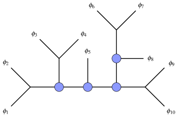
Figure 1: Choice of an OPE channel for a 10-point function. Vertices highlighted in blue are associated with non-trivial tensor structures.

Prerequisites and notation. Conformal correlation functions are symmetric with respect to the exchange of any two fields. On the other hand, the way we compute them is not. In fact, $N$-point correlation functions are evaluated by a repeated use of operator product expansions (OPEs) and the precise sequence of performing these expansions determines what is known as an OPE channel. These channels can be represented as (plane) tree diagrams $\mathcal{C}^{N}_{\textit{OPE}}$ with enumerated leaves. Figure 1 shows one such example for the 10-point function. Given a fixed enumeration of the external scalar fields, the number of OPE channels is $(2N-5)!!$. Each of these channels is associated with a system of conformal blocks that provide a Fourier-like expansion of the correlation function. After stripping off some appropriate prefactors $\Omega(x_{i}|\Delta_{i})$, the conformal blocks depend only on conformally invariant cross ratios. It is well known that one can form

$$n_{\textit{cr}}(N,d)=\left\{\begin{array}[]{ll}\frac{1}{2}N(N-3)&N\leq d+2\\[8.53581pt] Nd-\frac{1}{2}(d+2)(d+1)&N>d+2\end{array}\right.$$ (3)

of such independent cross ratios from a set of $N$ points $x_{i}\in\mathbb{R}^{d}$. Note that this number is independent of the OPE channel. The conformal blocks we want to expand our correlation functions in must depend on the same number of labels. For example, in the case of a 4-point function in $d>1$ one has two cross ratios. The associated blocks are famously labeled by the conformal weight $\Delta$ and the spin $l$ of the field that is exchanged in the intermediate channel. Since the latter transforms in a symmetric traceless tensor representation of the rotation subgroup, a single number $l$ is sufficient to characterize the spin.

When dealing with higher correlation functions, it is easy to see that the quantum numbers of fields exchanged in the intermediate channels are not sufficient. The precise number of such intermediate field labels does depend on the channel topology, at least for $N>5$, but it is always strictly smaller than the number $n_{\textit{cr}}$ of cross ratios. As an example let us consider $N=5$.

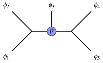
Figure 2: Choice of OPE diagram for 5-point correlator.

In this case there exist $15$ OPE channels but they all possess the same topology. In Figure 2 we have displayed one of the fifteen OPE channels. All other 14 channels are related to this one by a permutation of the leaves, modulo symmetries of the bare OPE diagram that has been stripped of its leaves. As one can readily see, the OPE evaluation involves two intermediate fields. Since these appear in the operator product of scalar fields, they are symmetric traceless tensors and hence characterized by two quantum numbers each. The intermediate fields thus carry four quantum numbers in total. We think of these as being attached to the (internal) links of the OPE diagram. But in order to fully characterize the relevant blocks we need five quantum numbers and so we are short by one. As we shall show below, this remaining quantum number is attached to the central vertex of the 5-point OPE diagram. Note that two legs of this central vertex are associated with a symmetric traceless tensor while only one is scalar. For $d\geq 3$, such 3-point functions are not determined by conformal symmetry. They require the choice of a so-called tensor structure. For a very particular basis in the space of tensor structures it becomes possible to assign a fifth quantum number to the choice of tensor structure, one that can be measured simultaneously with the four independent eigenvalues of the Casimir operators. Measuring a complete set of quantum numbers simultaneously through a sufficiently large set of commuting differential operators is the main goal of this work. We want to do so in any $d$, for any number $N$ of external points and for all OPE channels. Quantum numbers are measured by acting with differential operators in the cross ratios. The latter divide into two families. First, differential operators that measure the quantum numbers of intermediate fields are associated with the links of the OPE diagram and are referred to as Casimir differential operators, since they are straightforward generalizations of the Casimir differential operators constructed for $N=4$ by Dolan and Osborn. Second, differential operators that measure choices of tensor structure, the first example of which was introduced recently in Buric:2020dyz , are referred to as vertex differential operators. Let us note that for scalar blocks, the choice of tensor structures and hence the vertex differential operators are relevant as soon as multiple non-scalar exchanges are involved. These types of blocks have only been considered very recently in Poland:2021xjs and (Goncalves:2019znr, , Appendix E) for five-point blocks, and in a certain limit in Vieira:2020xfx for five or six scalar legs.

Before we can describe our results on both types of differential operators we need to set up some notation. Given an OPE channel we enumerate internal lines by Latin indices $r=1,\dots,N-3$ and vertices by Greek indices $\rho=1,\dots,N-2$. There are no rules on how to enumerate these two sets of objects. OPE diagrams are (plane) trees and hence by cutting any internal line with label $r$ we separate the diagram into two disconnected pieces. Hence, $r$ is associated with a partition of the external fields into two disjoint sets,

$$\underline{N}=\{1,\dots,N\}=I_{r,1}\mathbin{\mathchoice{\leavevmode\vtop{\halign{\hfil$\m@th\displaystyle#$\hfil\cr\cup\cr\cdot\crcr}}}{\leavevmode\vtop{\halign{\hfil$\m@th\textstyle#$\hfil\cr\cup\cr\cdot\crcr}}}{\leavevmode\vtop{\halign{\hfil$\m@th\scriptstyle#$\hfil\cr\cup\cr\cdot\crcr}}}{\leavevmode\vtop{\halign{\hfil$\m@th\scriptscriptstyle#$\hfil\cr\cup\cr\cdot\crcr}}}}I_{r,2}\ .$$ (4)

Similarly, any vertex $\rho$ gives rise to a partition of $\underline{N}$ into three disjoint sets

$$\underline{N}=I_{\rho,1}\mathbin{\mathchoice{\leavevmode\vtop{\halign{\hfil$\m@th\displaystyle#$\hfil\cr\cup\cr\cdot\crcr}}}{\leavevmode\vtop{\halign{\hfil$\m@th\textstyle#$\hfil\cr\cup\cr\cdot\crcr}}}{\leavevmode\vtop{\halign{\hfil$\m@th\scriptstyle#$\hfil\cr\cup\cr\cdot\crcr}}}{\leavevmode\vtop{\halign{\hfil$\m@th\scriptscriptstyle#$\hfil\cr\cup\cr\cdot\crcr}}}}I_{\rho,2}\mathbin{\mathchoice{\leavevmode\vtop{\halign{\hfil$\m@th\displaystyle#$\hfil\cr\cup\cr\cdot\crcr}}}{\leavevmode\vtop{\halign{\hfil$\m@th\textstyle#$\hfil\cr\cup\cr\cdot\crcr}}}{\leavevmode\vtop{\halign{\hfil$\m@th\scriptstyle#$\hfil\cr\cup\cr\cdot\crcr}}}{\leavevmode\vtop{\halign{\hfil$\m@th\scriptscriptstyle#$\hfil\cr\cup\cr\cdot\crcr}}}}I_{\rho,3}\ .$$ (5)

Given any subset $I\subset\underline{N}$ we can define the following set of first order differential operators in the insertion points $x_{i}$,

$$\mathcal{T}^{(I)}_{\alpha}=\sum_{i\in I}\mathcal{T}^{(i)}_{\alpha}\ .$$ (6)

Let us note that for two disjoint sets $I_{1},I_{2}\subset\underline{N}$ we have

$$\mathcal{T}^{(I_{1}\mathbin{\mathchoice{\leavevmode\vtop{\halign{\hfil$\m@th\displaystyle#$\hfil\cr\cup\cr\cdot\crcr}}}{\leavevmode\vtop{\halign{\hfil$\m@th\textstyle#$\hfil\cr\cup\cr\cdot\crcr}}}{\leavevmode\vtop{\halign{\hfil$\m@th\scriptstyle#$\hfil\cr\cup\cr\cdot\crcr}}}{\leavevmode\vtop{\halign{\hfil$\m@th\scriptscriptstyle#$\hfil\cr\cup\cr\cdot\crcr}}}}I_{2})}_{\alpha}=\mathcal{T}^{(I_{1})}_{\alpha}+\mathcal{T}^{(I_{2})}_{\alpha}\ ,\quad[\,\mathcal{T}^{(I_{1})}_{\alpha}\,,\,\mathcal{T}^{(I_{2})}_{\beta}\,]=0\ .$$ (7)

Casimir differential operators. With this notation it is very easy to construct the differential operators that measure the quantum numbers of the intermediate fields,

$$\mathcal{C}\textit{\!as\,}^{p}_{r}=\mathcal{D}^{p}_{r,1}=\kappa_{p}^{\alpha_{1},\dots,\alpha_{p}}\left[\mathcal{T}^{(I_{r,1})}_{\alpha_{1}}\cdots\mathcal{T}^{(I_{r,1})}_{\alpha_{p}}\right]_{|\mathcal{G}}=\mathcal{D}^{p}_{r,2}\ .$$ (8)

Here $\kappa_{p}$ denotes symmetric conformally invariant tensors of order $p$ and the superscript $p$ runs through

$$p=2,4,\dots\left\{\begin{array}[]{ll}d+1=2r_{d}&\textit{for $d$ odd}\\[5.69054pt] d=2r_{d}-2&\textit{for $d$ even}\end{array}\right.$$ (9)

The number $r_{d}=[(d+2)/2]$ denotes the rank of the conformal Lie algebra. In even dimensions $d$, the symmetric invariant tensor $\kappa_{p}$ of order $p=2r_{d}=d+2$ actually possesses a square root of order $p=r_{d}$ that also commutes with all generators of the conformal algebra. This so-called Pfaffian differential operator has the same form as in (8), but with a symmetric invariant tensor $\kappa_{p}$ of order $p=d/2+1$,

$$\mathcal{P}\textit{\!f\,}_{r}=\mathcal{D}^{d/2+1}_{r,1}=\kappa_{d/2+1}^{\alpha_{1},\dots,\alpha_{d/2+1}}\left[\mathcal{T}^{(I_{r,1})}_{\alpha_{1}}\cdots\mathcal{T}^{(I_{r,1})}_{\alpha_{d/2+1}}\right]_{|\mathcal{G}}=-(-1)^{d/2}\mathcal{D}^{d/2+1}_{r,2}\ .$$ (10)

When $d=4k+2$, the symmetric invariants of order $p=d/2+1$ are twofold degenerate and we should use two different symbols for these two invariants of order $d/2+1$. In order not to clutter notation too much, we decided to ignore this distinction. In other words, we will consider $\kappa_{d/2+1}$ as a pair of symmetric invariants when $d=4k+2$.

In our formulas for the differential operators we have placed a subscript $|\mathcal{G}$ to stress that they are defined as operators acting on correlations functions, i.e. on functions $\mathcal{G}$ that satisfy the conformal Ward identities

$$\mathcal{T}^{(\underline{N})}_{\alpha}\mathcal{G}_{N}(x_{i},\Delta_{i})=0\ .$$ (11)

In our construction of the differential operators we have favored the set $I_{r,1}$ over $I_{r,2}$. But from the conformal Ward identities we can conclude that

$$\mathcal{T}^{(I_{r,1})}_{\alpha}\mathcal{G}_{N}(x_{i},\Delta_{i})=-\mathcal{T}^{(I_{r,2})}_{\alpha}\mathcal{G}_{N}(x_{i},\Delta_{i})\ .$$

Though some caution is needed when we apply this relation to the evaluation of the Casimir differential operator, see Subsection 2.1 for details, it is not difficult to see that all differential operators of even order come out the same if we pick $I_{r,2}$ rather than $I_{r,1}$. There is only one family for which the set matters, namely for the Pfaffian operators when $d$ is a multiple of four. In that case the operator flips sign when we change the set. Of course, overall factors are a matter of convention and hence of no concern. Therefore, we shall drop the reference to the set we use in the construction of Casimir differential operators, writing $\mathcal{D}^{p}_{r}$ instead of $\mathcal{D}^{p}_{r,1}$.

An important point to note is that the Casimir differential operators need not be independent. To illustrate this, consider the case $N=4$ for $d>2$. Since all external fields are assumed to be scalar, the single intermediate field is a symmetric traceless tensor and is hence characterized by two numbers only, its weight $\Delta$ and spin $l$. These can be measured by the Casimir differential operators $\mathcal{D}^{2}$ and $\mathcal{D}^{4}$. But starting from $d=4$, the conformal algebra possesses Casimir elements of higher order which are independent in general, but become dependent on the lower order ones when evaluated on symmetric traceless tensors. More generally, the number of independent Casimir differential operators at a given internal line $r$ is given by

$$\mathfrak{d}_{r}(\mathcal{C}^{N}_{\textit{OPE}},d)=\mathfrak{d}(I_{r,1},d),\quad\textit{where}\quad\mathfrak{d}(I,d)=\textit{min}(|I|,N-|I|,r_{d}),$$ (12)

and $|I|$ denotes the order of the set $I$. We shall refer to the number $\mathfrak{d}(I,d)$ as the depth of the index set $I$ and to $\mathfrak{d}_{r}$ as the depth of the link $r$. Note that $\mathfrak{d}_{r}=\mathfrak{d}(I_{r,1},d)=\mathfrak{d}(I_{r,2},d)$ is independent of which of the two index sets we choose to compute it with. By summing the depths of all internal links, we can determine the total number of independent Casimir differential operators to be

$$n_{\textit{cdo}}(\mathcal{C}^{N}_{\textit{OPE}},d)=\sum_{r=1}^{N-3}\mathfrak{d}_{r}(\mathcal{C}^{N}_{\textit{OPE}},d)\ .$$ (13)

Let us note that the total number of Casimir differential operators does depend on the topology of the OPE channel, not just on the number $N$ of points. In the case of $N=6$ and $d\geq 4$, for example, there are $n_{\textit{cdo}}(\mathcal{C}^{N=6}_{\textit{comb}},d)=7$ Casimir differential operators in the comb channel, while the snowflake channel admits only $n_{\textit{cdo}}(\mathcal{C}^{N=6}_{\textit{snowflake}},d)=6$ of such operators.

Vertex differential operators. What we have described so far is nothing new, and can be established by elementary means. But as we have explained, starting from $N=5$ the Casimir differential operators do not suffice to resolve all quantum numbers of the conformal blocks, i.e. $n_{\textit{cdo}}$ is strictly smaller that $n_{\textit{cr}}$ for all OPE channels. Our main task is to construct additional differential operators that can measure the choice of tensor structures at the vertices independently of the weights and spins of the intermediate fields, i.e. we need to find a complete set of vertex differential operators that commute with the Casimir differential operators and among themselves. In this work we describe how to accomplish this task, for any number $N$ of external scalar fields and any OPE topology. One central claim is that these vertex differential operators take the form

$$\mathcal{D}^{p,\nu}_{\rho,12}=\kappa_{p}^{\alpha_{1},\dots,\alpha_{\nu},\alpha_{\nu+1},\dots,\alpha_{p}}\left[\mathcal{T}^{(I_{\rho,1})}_{\alpha_{1}}\cdots\mathcal{T}^{(I_{\rho,1})}_{\alpha_{\nu}}\mathcal{T}^{(I_{\rho,2})}_{\alpha_{\nu+1}}\cdots\mathcal{T}^{(I_{\rho,2})}_{\alpha_{p}}\right]_{|\mathcal{G}}$$ (14)

where $\nu=1,\dots,p-1$ and $p=2,4,\dots,2r_{d}=d+1$ when $d$ is odd. For even $d$, we let $p$ run through even integers until we reach $d$ and add a set of Pfaffian vertex operators $\mathcal{P}\textit{f\;}^{\nu}_{\rho,12},\nu=1,2,\dots d/2$ which are constructed with a symmetric invariant tensor $\kappa_{p}$ of order $p=d/2+1$. Let us note that the definition of all these vertex differential operators also makes sense for $\nu=0$ and $\nu=p$. The corresponding objects coincide with Casimir differential operators for the links that enter the first and second leg of the vertex. This is why we have excluded them from our list. The remaining operators still allow us to reconstruct the Casimir operators for the link that enters the third leg. Therefore, there is one linear relation for each value that $p$ can assume, i.e. we have $r_{d}$ linear relations in total. One may use these relations to eliminate e.g. the operator with $\nu=p/2$.

Let us note that the definition of the vertex operators $\mathcal{D}^{p,\nu}_{\rho,ij}$ depends on the choice of labeling of the subsets $I_{\rho,j}$ forming the partition $\underline{N}=I_{\rho,1}\mathbin{\mathchoice{\leavevmode\vtop{\halign{\hfil$\m@th\displaystyle#$\hfil\cr\cup\cr\cdot\crcr}}}{\leavevmode\vtop{\halign{\hfil$\m@th\textstyle#$\hfil\cr\cup\cr\cdot\crcr}}}{\leavevmode\vtop{\halign{\hfil$\m@th\scriptstyle#$\hfil\cr\cup\cr\cdot\crcr}}}{\leavevmode\vtop{\halign{\hfil$\m@th\scriptscriptstyle#$\hfil\cr\cup\cr\cdot\crcr}}}}I_{\rho,2}\mathbin{\mathchoice{\leavevmode\vtop{\halign{\hfil$\m@th\displaystyle#$\hfil\cr\cup\cr\cdot\crcr}}}{\leavevmode\vtop{\halign{\hfil$\m@th\textstyle#$\hfil\cr\cup\cr\cdot\crcr}}}{\leavevmode\vtop{\halign{\hfil$\m@th\scriptstyle#$\hfil\cr\cup\cr\cdot\crcr}}}{\leavevmode\vtop{\halign{\hfil$\m@th\scriptscriptstyle#$\hfil\cr\cup\cr\cdot\crcr}}}}I_{\rho,3}$ associated with the vertex $\rho$, which is arbitrary. However, the algebra generated by the vertex operators $\mathcal{D}^{p,\nu}_{\rho}$ is in fact independent of this choice: more precisely, the vertex operators constructed from another choice of labeling of the $I_{\rho,j}$’s are linear combinations of the operators $\mathcal{D}^{p,\nu}_{\rho,12}$, modulo the use of the conformal Ward identities (11), see Section 2.2.

The number of vertex differential operators at a given vertex is now easy to count. Taking into account that one additional linear relation among the operators listed in eq. (14), one finds

$$n_{v}(d)=\left\{\begin{array}[]{ll}\frac{1}{4}(d^{2}-4)&\textit{for d even}\\[5.69054pt] \frac{1}{4}(d^{2}-1)&\textit{for d odd}\end{array}\right.$$ (15)

The first key result of this work is that these vertex differential operators commute among themselves and with the Casimir differential operators. Commutation between Casimir and vertex differential operators is obvious. Similarly, it is easy to show that two vertex operators commute if they are associated with different vertices $\rho\neq\rho^{\prime}$. The deepest part of our claim concerns the fact that also vertex operators associated with the same vertex commute. It does not seem straightforward to prove this statement by elementary manipulations. Below we shall use an indirect strategy in which we identify these vertex differential operators with Hamiltonians of some Gaudin integrable system defined on a 3-punctured sphere. For the latter, commutativity has already been established.

Of course the vertex differential operators we listed may not all be independent, as for the Casimir operators, see discussion above. In order to count the number of independent vertex differential operators, we shall employ the depth function $\mathfrak{d}(I,d)$ we introduced in eq. (12). For a given vertex $\rho$ inside an OPE channel $\mathcal{C}^{N}_{\textit{OPE}}$, the number of independent vertex differential operators is expected to be equal to the degrees of freedom associated to this vertex

$$n_{\textit{vdo},\rho}(\mathcal{C}^{N}_{\textit{OPE}},d)=n_{\textit{cr}}(\sum_{i=1}^{3}\mathfrak{d}_{\rho,i},d)-\sum_{i=1}^{3}\mathfrak{d}_{\rho,i}(\mathfrak{d}_{\rho,i}-1)\leq n_{v}(d)$$ (16)

where $\mathfrak{d}_{\rho,i}=\mathfrak{d}(I_{\rho,i},d)$ with $i=1,2,3$. The inequality is saturated for vertices $\rho$ with $\mathfrak{d}_{\rho,i}=r_{d}$. For the special vertices that can appear in the comb channel and in which one of the legs is scalar, the formula becomes

$$n_{\textit{vdo},\rho_{m}}=m-1\ ,\quad n_{\textit{vdo},\rho_{r_{d}}}=r_{d}-1-\delta_{d,\textit{even}}$$

for $m=1,\dots,r_{d}-1$. Here $\rho_{m}$ is a vertex with $\mathfrak{d}_{\rho_{m},1}=m,\mathfrak{d}_{\rho_{m},2}=1$ and $\mathfrak{d}_{\rho_{m},3}=m+1$, see Figure 3, and $\rho_{d}$ is the maximal comb channel vertex with $\mathfrak{d}_{\rho_{r_{d}},1}=r_{d}=\mathfrak{d}_{\rho_{r_{d}},3}$. The total number $n_{\textit{vdo}}(\mathcal{C}^{N}_{\textit{OPE}},d)$ of vertex differential operators is obtained by summing over all $N-2$ vertices, i.e.

$$n_{\textit{vdo}}(\mathcal{C}^{N}_{\textit{OPE}},d)=\sum_{\rho=1}^{N-2}n_{\textit{vdo},\rho}(\mathcal{C}^{N}_{\textit{OPE}},d)\ .$$

At least for the comb channel, it is easy to verify that the number of independent Casimir and vertex differential operators coincides with the number of cross ratios,

$$n_{\textit{cdo}}(\mathcal{C}^{N}_{\textit{OPE}},d)+n_{\textit{vdo}}(\mathcal{C}^{N}_{\textit{OPE}},d)=n_{\textit{cr}}(N,d)\ .$$

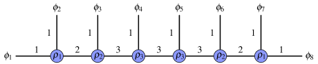
Figure 3: OPE diagram in the comb channel for a scalar eight-point function in $d=4$. The edge labels correspond to the depth $\mathfrak{d}$ of the associated links. When taking an OPE with a scalar field, the depth always increases by one until the maximal allowed depth $\mathfrak{d}=r_{d}$ is reached.

The formula holds of course for all OPE channels. Below we shall exhibit the relations among vertex differential operators that are responsible for the reduction from the $n_{v}(d)$ operators in our list (14) (with $\nu=p/2$ removed) to the $n_{\textit{vdo},\rho}(\mathcal{C}^{N}_{\textit{OPE}},d)$ independent vertex differential operators that are needed to characterize the vertex $\rho$. This is the second key result of this work. It will allow us in particular to determine the precise order of each independent vertex differential operator.

While Gaudin models for the 3-punctured sphere only enter the discussion as a convenient tool to construct commuting vertex differential operators at the individual vertices, the relation between conformal blocks and Gaudin models turns out to reach much further. In fact, is is possible to embed the whole set of Casimir and vertex differential operators for arbitrary scalar $N$-point functions into Gaudin models on the $N$-punctured sphere. The latter contains $N$ additional complex parameters that are not present in correlation functions. In the Gaudin integrable model these parameters correspond to the poles of the Lax matrix and they enter all Gaudin Hamiltonians. By considering different limiting configurations of these parameters is is possible to recover the full set of Casimir and vertex differential operators for scalar $N$-point functions in all the OPE channels. This construction not only embeds our differential operators into a unique Gaudin integrable model, but also shows that operators in different channels are related by a smooth deformation.

Let us finally outline the content of the following sections. Section 2 is mostly devoted to the study of the individual vertices. After a brief discussion of commutativity for Casimir differential operators and also vertex differential operators assigned to different vertices, we shall zoom into the individual vertices for most of Section 2. In Section 2.2 we construct the vertex differential operators in terms of the commuting Hamiltonians of a 3-site Gaudin integrable system. Section 2.3 addresses the relations between these operators for restricted vertices. The main purpose of Section 3 is to embed the whole set of Casimir and vertex differential operators for arbitrary scalar $N$-point functions into Gaudin models on the $N$-punctured sphere. In Section 4 we discuss one concrete example, namely we construct all five differential operators that characterize the blocks of a scalar 5-point function in any $d\geq 3$. Two of these operators are of order two while the other three are of fourth order. The paper concludes with a summary, outlook to further results and a list of interesting open problems to be addressed.

2 The Vertex Integrable System

The aim of this section is to address the key new element in the construction of multi-point conformal blocks for $d\geq 3$: the vertices themselves. In the first subsection we shall show that the construction of commuting differential operators for scalar $N$-point blocks can be reduced by rather elementary arguments to the construction of commuting differential operators for 3-point functions of spinning fields. Recall that the dependence on spin degrees of freedom can be encoded in auxiliary variables from which one is often able to construct non-trivial cross ratios, even in the case of a 3-point function. Constructing sufficiently many commuting vertex differential operators that act on such cross ratios of the 3-point function requires more powerful technology from integrability which we shall turn to in the second subsection. There we construct commuting differential operators for vertices from the Gaudin integrable model for the 3-punctured sphere. The basic construction provides $n_{v}(d)$ of such commuting operators and hence sufficiently many even for the most generic vertices. For special vertices, such as those appearing in the comb channel with external scalars, there exist linear relations between these operators. These are the subject of the third subsection.

2.1 Reduction to the vertex systems

Our goal here is to prove that Casimir and vertex operators constructed around different vertices of an OPE diagram commute. More precisely we shall show that

$$[\,\mathcal{D}^{p}_{r}\,,\,\mathcal{D}^{q}_{r^{\prime}}\,]=0\quad,\quad[\,\mathcal{D}^{p}_{r}\,,\,\mathcal{D}^{q,\nu}_{\rho,a}\,]=0$$ (17)

for every pair $(r,p),(r^{\prime},q)$ of Casimir operators and any choice $(\rho,q,\nu)$ of a vertex operator, including the Pfaffian Casimir and vertex operators that appear at order $p,q=d/2+1$ when the dimension $d$ is even. Note that the individual vertex differential operators also depend on the choice $a\in\{12,23,13\}$ of a pair of legs. In addition, we shall also establish that vertex operators associated with different vertices commute,

$$[\,\mathcal{D}^{p,\nu}_{\rho,a}\,,\,\mathcal{D}^{q,\mu}_{\rho^{\prime},b}\,]=0\quad\mathit{for}\ \rho\neq\rho^{\prime}$$ (18)

and all triples $(p,\nu,a)$ and $(q,\mu,b)$. This leaves only the commutativity of operators attached to the same vertex which is deferred to the next subsection.

The properties (17) and (18) are in fact elementary. They require global conformal invariance, the tree structure of OPE diagrams and the commutativity property (7). To begin with, let us recall that we associated two disjoint sets $I_{r,1}$ and $I_{r,2}$ to every link. As we pointed out before, the Casimir differential operators (8) do not depend on whether we used the generators $\mathcal{T}_{\alpha}^{(I_{r,1})}$ or $\mathcal{T}_{\alpha}^{(I_{r,2})}$ to construct them. Let us briefly discuss the details of the proof. Note that we think of $\mathcal{D}$ as an operator acting on correlation functions $\mathcal{G}$. This is signaled by the subscript $|\mathcal{G}$ in the definition of the Casimir differential operators. In evaluating products of first order differential operators, one can only apply the Ward identity (11) to the rightmost operator, which acts directly on the correlation function, and not on some derivative thereof. But once we have converted the rightmost operators $\mathcal{T}^{(I_{r,1})}$ into $-\mathcal{T}^{(I_{r,2})}$, they will commute with all operators to their left, such that we can freely move them all the way to the left and proceed to apply the Ward identity to the next set of first order operators, and so on. If we finally take into account that the invariants $\kappa$ of the conformal Lie algebra are symmetric, we arrive at an expression for the Casimir differential operators in terms of $\mathcal{T}^{(I_{r,2})}$.

A similar analysis can be carried out for vertex operators, see also Subsection 2.2. Without loss of generality we can assume that we have constructed our vertex operators in terms of the generators $\mathcal{T}^{(I_{\rho,1})}$ and $\mathcal{T}^{(I_{\rho,2})}$ and want to switch to constructing them from $\mathcal{T}^{(I_{\rho,1})}$ and $\mathcal{T}^{(I_{\rho,3})}$ instead. To do so we make use of the invariance condition

$$\left[\mathcal{T}^{(I_{\rho,2})}_{\alpha}\right]_{|\mathcal{G}}=-\left[\mathcal{T}^{(I_{\rho,1})}_{\alpha}-\mathcal{T}^{(I_{\rho,3})}_{\alpha}\right]_{|\mathcal{G}}\$$ (19)

that follows from relations (5) and (11). After we apply this to the rightmost operator in the vertex differential operator, we use the commutativity property (7) to move the generators $\mathcal{T}^{(I_{\rho,1})}$ and $\mathcal{T}^{(I_{\rho,3})}$ to the left of $\mathcal{T}^{(I_{\rho,2})}$. We continue this replacement process until all the generators $\mathcal{T}^{(I_{\rho,2})}$ are removed and using symmetry of the tensor $\kappa$ we find

$$\mathcal{D}^{p,\nu}_{\rho,12}=(-1)^{p-\nu}\sum_{\mu=0}^{p-\nu}\binom{p-\nu}{\mu}\mathcal{D}^{p,\nu+\mu}_{\rho,13}$$ (20)

along with a similar relation for the Pfaffian vertex operators for $p=d/2+1$ and $d$ even. Since the last term in this sum with $\mu=p-\nu$ is just a Casimir operator, we have managed to express all vertex differential operators that are constructed from the generators associated with $I_{\rho,1}$ and $I_{\rho,2}$ as a linear combination of the vertex operators associated with the pair $I_{\rho,1}$ and $I_{\rho,3}$ and a Casimir operator. This is the main input in proving the commutativity statements (17) and (18).

Let us start with a pair of links $r,r^{\prime}$. Each of these links divides the set of external points into the two disjoint sets $I_{r,1},I_{r,2}$ and $I_{r^{\prime},1},I_{r^{\prime},2}$ respectively. Since the OPE diagram is a tree, it is always possible to find a pair $i,j=1,2$ such that $I_{r,i}\cap I_{r^{\prime},j}=\emptyset$. For this choice

$$[\,\mathcal{D}^{p}_{r}\,,\,\mathcal{D}^{q}_{r^{\prime}}\,]=[\,\mathcal{D}^{p}_{r,i}\,,\,\mathcal{D}^{q}_{r^{\prime},j}\,]=0$$ (21)

because of the commutativity property (7). This proves our first claim. Note that the same arguments also apply to the case in which $r=r^{\prime}$ and also if one or both operators are Pfaffian, i.e. if $d$ is even and $p,q=d/2+1$.

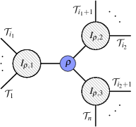
Figure 4: Schematic representation of a generic OPE diagram with focus on one vertex. The choice of a vertex automatically divides the diagram into three branches.

Let us now extend this argument to include vertex differential operators. In order to prove that the Casimir operators associated to a link $r$ commute with the vertex operators associated to any vertex $\rho$ we recall that any choice of a vertex $\rho$ on an OPE diagram divides the diagram into the three distinct branches that are glued to the vertex, and we denote these by $I_{\rho,j}$ as in Figure 4. A quick glance at Figure 4 suffices to conclude that given $r$ and $\rho$ it is possible to find a pair $i\in{1,2}$ and $j\in{1,2,3}$ such that $I_{r,i}\subset I_{\rho,j}$, since the link $r$ must be in one of the three branches. It follows that $I_{r,i}\cap\left(I_{\rho,j_{1}}\cup I_{\rho,j_{2}}\right)=\emptyset$ for $j_{1}\neq j\neq j_{2}$. Commutativity of Casimir and vertex differential operators then follows since we can construct the Casimir differential operators in terms of the generators for $I_{r,i}$ while using the generators for $I_{\rho,j_{1}}$ and $I_{\rho,j_{2}}$ for the vertex differential operators.

Figure 5: Schematic representation of a generic OPE diagram with focus on two internal vertices. Operators supported around distinct vertices trivially commute, as they can be written in terms of generators that belong to different branches.

Let us finally consider any two distinct vertices $\rho$ and $\rho^{\prime}$ on an OPE diagram. As we highlight in Figure 5, any configuration of two vertices divides the diagram into five parts: four external branches $I_{\rho,j}$, $I_{\rho^{\prime},j}$, $j=1,2$, attached to only one vertex, and the central part $\mathcal{C}$ of the diagram that is attached to both vertices $\rho$ and $\rho^{\prime}$. Following what we just claimed with focus on one vertex, we can use diagonal conformal symmetry to rewrite the operators around $\rho$ and $\rho^{\prime}$ to depend on disjoint sets of legs $I_{\rho,j}$, $I_{\rho^{\prime},j}$ with $j=1,2$. Since generators associated to these sets commute (7), it follows automatically that operators constructed around different vertices must commute as well.

This implies that to prove commutativity of our set of operators, we can just focus on operators that live around one single vertex. To prove the commutativity of these vertex operators we will now make use of the integrability technology that is provided by Gaudin models.

2.2 The vertex system and Gaudin models

In this section, we will explain how the operators (14) associated with a vertex $\rho$ in the OPE diagram naturally arise from a specific Gaudin model, which in particular will provide us with a proof of their commutativity. Let us start by reviewing briefly how Gaudin models are defined Gaudin_76a ; Gaudin_book83 . They are integrable systems naturally constructed from a choice of a simple Lie algebra $\mathfrak{g}$. Having in mind applications of these systems to conformal field theories, we will choose $\mathfrak{g}$ to be the conformal Lie algebra $\mathfrak{so}(d+1,1)$ of the Euclidean space $\mathbb{R}^{d}$, with basis $T_{\alpha}$ as in the previous section. The Gaudin model depends in general on $M$ complex numbers $w_{j}$, called its sites, to which are attached $M$ independent representations of the algebra $\mathfrak{g}$. To obtain the vertex system we address in this section, we restrict our attention here to the case $M=3$ and associate with these three sites the representations of $\mathfrak{g}$ corresponding to the three fields attached to the vertex $\rho$. More precisely, using the notation defined in Section 1 and in particular the partition $\underline{N}=I_{\rho,1}\mathbin{\mathchoice{\leavevmode\vtop{\halign{\hfil$\m@th\displaystyle#$\hfil\cr\cup\cr\cdot\crcr}}}{\leavevmode\vtop{\halign{\hfil$\m@th\textstyle#$\hfil\cr\cup\cr\cdot\crcr}}}{\leavevmode\vtop{\halign{\hfil$\m@th\scriptstyle#$\hfil\cr\cup\cr\cdot\crcr}}}{\leavevmode\vtop{\halign{\hfil$\m@th\scriptscriptstyle#$\hfil\cr\cup\cr\cdot\crcr}}}}I_{\rho,2}\mathbin{\mathchoice{\leavevmode\vtop{\halign{\hfil$\m@th\displaystyle#$\hfil\cr\cup\cr\cdot\crcr}}}{\leavevmode\vtop{\halign{\hfil$\m@th\textstyle#$\hfil\cr\cup\cr\cdot\crcr}}}{\leavevmode\vtop{\halign{\hfil$\m@th\scriptstyle#$\hfil\cr\cup\cr\cdot\crcr}}}{\leavevmode\vtop{\halign{\hfil$\m@th\scriptscriptstyle#$\hfil\cr\cup\cr\cdot\crcr}}}}I_{\rho,3}$ constructed from the vertex $\rho$, we will attach to the three sites $w_{j}$, $j=1,2,3$, of the Gaudin model the generators $\mathcal{T}_{\alpha}^{(I_{\rho,j})}$ which define representations of $\mathfrak{g}$ in terms of first-order differential operators in the insertion points $x_{i}$.

A key ingredient in the construction of the Gaudin model is its so-called Lax matrix, whose components in the basis $T^{\alpha}$ are defined here as

$$\mathcal{L}^{\rho}_{\alpha}(z)=\sum_{j=1}^{3}\frac{\mathcal{T}_{\alpha}^{(I_{\rho,j})}}{z-w_{j}},$$ (22)

where $z$ is an auxiliary complex variable called the spectral parameter. In the above equation, we have denoted the Lax matrix as $\mathcal{L}^{\rho}_{\alpha}(z)$ to emphasize that this is the matrix corresponding to the vertex $\rho$. For any elementary symmetric invariant tensor $\kappa_{p}$ of degree $p$ on $\mathfrak{g}$, there is a corresponding $z$-dependent Gaudin Hamiltonian of the form

$$\mathcal{H}^{(p)}_{\rho}(z) = \kappa_{p}^{\alpha_{1}\cdots\alpha_{p}}\mathcal{L}_{\alpha_{1}}^{\rho}(z)\cdots\mathcal{L}_{\alpha_{p}}^{\rho}(z)+\dots,$$ (23)

where $\dots$ represent quantum corrections, involving a smaller number of components of the Lax matrix $\mathcal{L}_{\alpha}^{\rho}$ and their derivatives with respect to $z$. These corrections are chosen specifically to ensure that the Gaudin Hamiltonians commute for all values of the spectral parameter and all degrees:

$$\bigl{[}\mathcal{H}_{\rho}^{(p)}(z),\mathcal{H}_{\rho}^{(q)}(w)\bigr{]}=0,\qquad\forall\,z,w\in\mathbb{C},\quad\forall\,p,q\ .$$ (24)

The existence of such commuting Hamiltonians was first proven in Feigin:1994in , using some previously established results Feigin:1991wy on the so-called Feigin-Frenkel center of affine algebras at the critical level. The explicit expression for the quantum corrections was obtained in Talalaev:2004qi ; Chervov:2006xk for Lie algebras of type A and in Molev:2013 for types B, C, D, which is the case we are concerned with here (indeed, $\mathfrak{g}=\mathfrak{so}(d+1,1)$ is of type B for $d$ odd and of type D for $d$ even). We refer to Molev:2018 for a summary of these results. The properties of the Feigin-Frenkel center were further studied in the recent work Yakimova:2019 , the results of which imply that the quantum corrections in $\mathcal{H}^{(p)}_{\rho}(z)$ are sums of terms of the form

$$\tau^{\alpha_{1}\cdots\alpha_{q}}\;\partial_{z}^{r_{1}-1}\mathcal{L}^{\rho}_{\alpha_{1}}(z)\cdots\partial_{z}^{r_{q}-1}\mathcal{L}^{\rho}_{\alpha_{q}}(z),$$ (25)

where $q<p$, $\tau^{\alpha_{1}\cdots\alpha_{q}}$ is a completely symmetric invariant tensor of degree $q$ on $\mathfrak{g}$ and $r_{1},\cdots,r_{q}$ are positive integers such that $r_{1}+\cdots+r_{q}=p$. For what follows, it will be useful to consider the leading part of the Hamiltonian (23) alone, without quantum corrections, which we will denote as

$$\widehat{\mathcal{H}}^{(p)}_{\rho}(z)=\kappa^{\alpha_{1}\cdots\alpha_{p}}\mathcal{L}_{\alpha_{1}}^{\rho}(z)\cdots\mathcal{L}_{\alpha_{p}}^{\rho}(z)\ .$$ (26)

Let us finally note that the quantum corrections are absent for both the quadratic Hamiltonian $\mathcal{H}^{(2)}_{\rho}(z)$ and the Pfaffian Hamiltonian $\mathcal{H}^{(d/2+1)}_{\rho}(z)$ that exists for $d$ even, such that these two Hamiltonians coincide with their leading parts.

To make the link with the vertex operators defined in Section 1, we will make a specific choice of the parameters $w_{j}$ of the Gaudin model. More precisely, we set

$$w_{1}=0,\qquad w_{2}=1\qquad\text{ and }\qquad w_{3}=\infty\ .$$ (27)

In particular, the Lax matrix (22) reduces to

$$\mathcal{L}^{\rho}_{\alpha}(z)=\frac{\mathcal{T}_{\alpha}^{(I_{\rho,1})}}{z}+\frac{\mathcal{T}_{\alpha}^{(I_{\rho,2})}}{z-1}\ .$$ (28)

Let us now study the Gaudin Hamiltonians $\mathcal{H}^{(p)}_{\rho}(z)$ for this particular choice of parameters. We will first focus on their leading part $\widehat{\mathcal{H}}^{(p)}_{\rho}(z)$. Reinserting the above expression of the Lax matrix in eq. (26), we simply find

$$\widehat{\mathcal{H}}^{(p)}_{\rho}(z)=\sum_{\nu=0}^{p}\binom{p}{\nu}\,\frac{\mathcal{D}_{\rho,12}^{p,\nu}}{z^{\nu}(z-1)^{p-\nu}},$$ (29)

where $\mathcal{D}_{\rho,12}^{p,\nu}$ is the vertex operator defined in eq. (14). To obtain this expression, we have used the fact that $\mathcal{T}_{\alpha}^{(I_{\rho,1})}$ and $\mathcal{T}_{\beta}^{(I_{\rho,2})}$ commute to bring all $\mathcal{T}_{\alpha}^{(I_{\rho,1})}$’s to the left, as well as the symmetry of the tensor $\kappa_{p}^{\alpha_{1}\cdots\alpha_{p}}$ to relabel the Lie algebra indices as in eq. (14). Noting that the fractions $z^{-\nu}(z-1)^{\nu-p}$ for $\nu=0,\cdots,p$ are linearly independent functions of $z$, it is then clear that one can extract all the vertex operators $\mathcal{D}_{\rho,12}^{p,\nu}$ from $\widehat{\mathcal{H}}^{(p)}_{\rho}(z)$. Note that the “extremal” operators $\mathcal{D}_{\rho,12}^{p,0}$ and $\mathcal{D}_{\rho,12}^{p,p}$ coincide with the Casimir operators of the fields at the branches $I_{\rho,1}$ and $I_{\rho,2}$ of the vertex. The same equation also holds for the Pfaffian operators $\mathcal{H}^{(d/2+1)}_{\rho}(z)$.

Our goal in this section is to prove the commutativity of the vertex operators $\mathcal{D}_{\rho,12}^{p,\nu}$ using known results on Gaudin models. This would follow automatically from the commutativity (24) of the Gaudin Hamiltonians $\mathcal{H}_{\rho}^{(p)}(z)$ if these Hamiltonians contained the operators $\mathcal{D}_{\rho,12}^{p,\nu}$. But we have already proven above that the latter are naturally extracted from the leading parts $\widehat{\mathcal{H}}^{(p)}_{\rho}(z)$ of the Gaudin Hamiltonians, without the quantum corrections. These quantum corrections are in general crucial for the commutativity of the Hamiltonians. However, we shall prove below that the quantum corrections of the specific Gaudin model considered here can always be expressed in terms of lower-degree Hamiltonians, and can thus be discarded without breaking the commutativity property. In this case, the non-corrected Hamiltonians $\widehat{\mathcal{H}}^{(p)}_{\rho}(z)$ pairwise commute for all values of the spectral parameter and all degrees, thus demonstrating the desired commutativity of the vertex operators $\mathcal{D}_{\rho,12}^{p,\nu}$.

Let us then analyze these quantum corrections. Recall that they are composed of terms of the form (25). Reinserting the expression (28) of the Lax matrix for the present choice of parameters $w_{j}$ in this equation, we find that the quantum corrections contain only terms of the form

$$\tau^{\alpha_{1}\cdots\alpha_{q}}\;\mathcal{T}_{\alpha_{1}}^{(I_{\rho,1})}\cdots\mathcal{T}_{\alpha_{\nu}}^{(I_{\rho,1})}\mathcal{T}_{\alpha_{\nu+1}}^{(I_{\rho,2})}\cdots\mathcal{T}_{\alpha_{q}}^{(I_{\rho,2})},$$ (30)

with prefactors composed of powers of $z$ and $z-1$, and where $\tau^{\alpha_{1}\cdots\alpha_{q}}$ is a completely symmetric invariant tensor on $\mathfrak{g}$ of degree $q<p$, as in eq. (25). In particular, $\tau^{\alpha_{1}\cdots\alpha_{q}}$ decomposes as a product of elementary symmetric invariant tensors $\kappa_{k}$, symmetrized over the indices $\alpha_{i}$, with $k\leq q<p$. The correction in the above equation can thus be re-expressed as an algebraic combination of lower-degree vertex operators $\mathcal{D}_{\rho,12}^{k,\nu}$. Since these are the coefficients of the non-corrected Hamiltonian $\widehat{\mathcal{H}}^{(k)}_{\rho}(z)$, recursion on the degrees shows that the quantum corrections can indeed be expressed in terms of lower-degree Hamiltonians, as anticipated.

Let us end this subsection with a brief discussion on the role played by the choice of labeling of the branches $I_{\rho,1}$, $I_{\rho,2}$ and $I_{\rho,3}$ attached to the vertex $\rho$. As mentioned in Section 1, this choice is arbitrary but enters the definition (14) of the vertex operators $\mathcal{D}_{\rho,12}^{p,\nu}$, which in this case contain only the generators $\mathcal{T}_{\alpha}^{(I_{\rho,1})}$ and $\mathcal{T}_{\alpha}^{(I_{\rho,2})}$. In the context of the 3-sites Gaudin model considered in this subsection, this is related to the choice of positions $w_{j}$ of the sites made in eq. (27). In particular, the absence of generators $\mathcal{T}_{\alpha}^{(I_{\rho,3})}$ in the Gaudin Hamiltonians $\mathcal{H}^{(p)}(z)$ is due to the fact that we sent the site $w_{3}$ to infinity. One could have made another choice of labeling and constructed vertex operators $\mathcal{D}_{\rho,23}^{p,\nu}$ from the generators $\mathcal{T}_{\alpha}^{(I_{\rho,3})}$ and $\mathcal{T}_{\alpha}^{(I_{\rho,2})}$, for instance. The corresponding choice of positions of the sites would then be related to the initial one by the Möbius transformation that exchanges $0$ and $\infty$ and fixes $1$, i.e. the inversion $z\mapsto\frac{1}{z}$. More precisely, under such a transformation of the spectral parameter, the Lax matrix of the Gaudin model behaves as a 1-form on the Riemann sphere and satisfies

$$-\frac{1}{z^{2}}\mathcal{L}_{\alpha}^{\rho}\left(\frac{1}{z}\right)=-\frac{\mathcal{T}_{\alpha}^{(I_{\rho,1})}+\mathcal{T}_{\alpha}^{(I_{\rho,2})}}{z}+\frac{\mathcal{T}_{\alpha}^{(I_{\rho,2})}}{z-1}\ .$$ (31)

Acting on the correlation function $\mathcal{G}_{N}$, which satisfies the Ward identities (11), this Lax matrix then becomes

$$-\frac{1}{z^{2}}\mathcal{L}_{\alpha}^{\rho}\left(\frac{1}{z}\right)_{|\mathcal{G}}=\left[\frac{\mathcal{T}_{\alpha}^{(I_{\rho,3})}}{z}+\frac{\mathcal{T}_{\alpha}^{(I_{\rho,2})}}{z-1}\right]_{|\mathcal{G}},$$ (32)

and thus coincides with the Lax matrix from which one would build the vertex operators $\mathcal{D}_{\rho,23}^{p,\nu}$ with generators $\mathcal{T}_{\alpha}^{(I_{\rho,3})}$ and $\mathcal{T}_{\alpha}^{(I_{\rho,2})}$. This proves that the operators $\mathcal{D}_{\rho,23}^{p,\nu}$ can naturally be extracted from the generating functions

$$\frac{(-1)^{p}}{z^{2p}}\widehat{\mathcal{H}}_{\rho}^{(p)}\left(\frac{1}{z}\right)_{|\mathcal{G}}\ .$$ (33)

Using the expression (29) of $\widehat{\mathcal{H}}_{\rho}^{(p)}\left(z\right)$ in terms of the initial vertex operators $\mathcal{D}_{\rho,12}^{p,\nu}$, we thus get that the $\mathcal{D}_{\rho,23}^{p,\nu}$’s are linear combinations of the $\mathcal{D}_{\rho,12}^{p,\nu}$’s, as was demonstrated by direct computation in the previous subsection. Let us note that the use of the Ward identities was a crucial step in the above reasoning, as highlighted for instance by the subscript $\mathcal{G}$ in eq. (33). This step should be performed with care, in particular when using the Ward identities to replace $-\mathcal{T}_{\alpha}^{(I_{\rho,1})}-\mathcal{T}_{\alpha}^{(I_{\rho,2})}$ by $\mathcal{T}_{\alpha}^{(I_{\rho,3})}$ in the Hamiltonians (33). Indeed, one can use the Ward identities only for generators on the right. In order to do so, one thus has to commute generators to bring them to the right, replace them through the Ward identities and commute them back to their original place. Although this procedure can in general create non-trivial corrections, it can in fact be done freely in the case at hand: indeed, commuting operators $\mathcal{T}_{\alpha_{k}}^{(I_{\rho,j})}$ and $\mathcal{T}_{\alpha_{l}}^{(I_{\rho,j})}$ within the Hamiltonian $\widehat{\mathcal{H}}_{\rho}^{(p)}$ creates a term proportional to the structure constant $f_{\alpha_{k}\alpha_{l}}^{\hskip 17.0pt\beta}$, which vanishes when contracted with the symmetric tensor $\kappa_{p}^{\alpha_{1}\cdots\alpha_{p}}$. This ensures that the Hamiltonian (33) indeed serves as a generating function of the operators $\mathcal{D}_{\rho,23}^{p,\nu}$ built from $\mathcal{T}_{\alpha}^{(I_{\rho,3})}$ and $\mathcal{T}_{\alpha}^{(I_{\rho,2})}$. A similar reasoning applies for the other choices of labeling, by considering the appropriate Möbius transformations that permute the sites $0$, $1$ and $\infty$ of our 3-site Gaudin model.

2.3 Restricted vertices and relations between vertex operators

In the previous subsection we have shown that all of the operators listed in eq. (14) commute with each other. As we have pointed out before, we did not include operators with $\nu=0$ and $\nu=p$ in the list since these coincide with Casimir differential operators,

$$\mathcal{D}^{p,0}_{\rho,12}=\mathcal{D}^{p}_{r_{1}}\quad,\quad\mathcal{D}^{p,p}_{\rho,12}=\mathcal{D}^{p}_{r_{2}}\ .$$ (34)

Here $r_{i}$ denotes the link that is attached to the $i^{th}$ leg of the vertex $\rho$, i.e. for which $I_{r_{i},j}=I_{\rho,i}$ with either $j=1$ or $j=2$. The remaining $p-1$ operators satisfy one more linear relation since

$$\sum_{\nu=0}^{p}\binom{p}{\nu}\,\mathcal{D}^{p,\nu}_{\rho}=\mathcal{D}^{p}_{r_{3}}\ .$$ (35)

Let us note that this relation also applies to the Pfaffian vertex operators that exist for $p=d/2+1$ when $d$ is even. We have used this relation to drop one of the vertex differential operators. Once these obvious relations are taken care of, the total number of commuting vertex differential operators is given by eq. (15) and matches precisely the maximal number of cross ratios that can be associated to a single (generic) vertex, see upper bound of eq. (16) in the introduction. But restricted vertices carry fewer variables, so their corresponding differential operators (constructed in the previous section) must obey further relations. It is the main goal of this subsection to discuss these relations. We will also check that, once these are taken into account, the number of remaining vertex differential operators matches the number (16) of cross ratios at restricted vertices.

Our arguments are based on an important auxiliary result concerning the differential operators $\mathcal{T}^{(I)}_{\alpha}$ that are associated to some subset $I\subset\underline{N}$ of order $|I|\leq N/2$. To present this requires a bit of preparation. Up to this point there was no need to spell out the precise form of the symmetric invariant tensors $\kappa_{p}$ that we used to construct our differential operators. Now we need to be a bit more specific. As is well known, such tensors can be realized as symmetrized traces,

$$\kappa^{\alpha_{1}\cdots\alpha_{p}}_{p}=\textit{tr}\left(T^{(\,\alpha_{1}}\cdots T^{\alpha_{p}\,)}\right)=\textit{str}\left(T^{\alpha_{1}}\cdots T^{\alpha_{p}}\right)\ .$$ (36)

Here $T^{\alpha}$ denote the generators of the conformal Lie algebra and $(\dots)$ signal symmetrization with respect to the indices. In the following we shall use the symbol str to denote this symmetrized trace. The trace can be taken in any faithful representation. The simplest of such choices is to use the fundamental representation. In order to construct the associated symmetric invariants more explicitly, we shall replace the index $\alpha$ that enumerates the basis of the conformal algebra by a pair $\alpha=[AB]$ where $A,B$ run through $A,B=0,1,\dots,d+1$ with $T^{[AB]}=-T^{[BA]}$. In the fundamental representation, the matrix elements of these generators take the form

$$\bigl{(}T^{[AB]}_{f}\bigr{)}^{C}_{\;\;D}=\eta^{AC}\,\delta^{B}_{\ D}-\eta^{BC}\,\delta^{A}_{\ D}\ ,$$

where $\eta_{AB}$ is the Minkowski metric with signature $(d+1,1)$ and $\eta^{AB}$ is its inverse. This makes it now easy to compute $\kappa_{p}$ explicitly. The only issue arises in even $d$. In this case the symmetrized traces in the fundamental representation do not generate all the invariants. In order to obtain the missing invariant, one has to include the trace in a chiral representation. The standard construction employs the spinor representation in which generators $T^{[AB]}$ are represented as

$$\bigl{(}T^{[AB]}_{s}\bigr{)}^{\sigma}_{\;\;\tau}=\frac{1}{4}\,[\,\gamma^{A}\,,\,\gamma^{B}\,]^{\sigma}_{\;\;\tau}\ ,$$

where $\gamma^{A}$ are the $d+2$-dimensional $\gamma$ matrices and the matrix indices are $\sigma,\tau=1,\dots,2^{d/2+1}$. One can then project to a chiral spinor representation with the help of $\gamma_{c}\sim\gamma^{0}\cdots\gamma^{d+1}$.

Let us now introduce the symbol $\mathcal{T}^{(I)}$ to denote the following Lie-algebra valued differential operators

$$\mathcal{T}^{(I)}=T^{\alpha}\,\cdot\,\mathcal{T}^{(I)}_{\alpha}=\frac{1}{2}T^{[AB]}\,\cdot\,\mathcal{T}^{(I)}_{[AB]}\ .$$

Upon evaluation in some finite-dimensional representation, such as the fundamental or the spinor representation, these become matrix valued differential operators. With this notation we write our set (14) as

$$\mathcal{D}^{p,\nu}_{\rho,12}=\textit{str}_{f}\left(\underbrace{\mathcal{T}^{(I_{\rho,1})}...\mathcal{T}^{(I_{\rho,1})}}_{\nu}\underbrace{\mathcal{T}^{(I_{\rho,2})}...\mathcal{T}^{(I_{\rho,2})}}_{p-\nu}\right)_{|\mathcal{G}}$$ (37)

when $d$ is odd and the parameters $p$ and $\nu$ assume the values $p=2,4,\dots,d+1$ and $\nu=1,\dots,p-1$, as usual. For even dimension $d$, on the other hand, we use the symmetrized trace in the fundamental representation for $p=2,4,\dots,d$ and construct the missing Pfaffian vertex differential operators as

$$\mathcal{D}^{d/2+1,\nu}_{\rho,12}=\textit{str}_{s}\left(\underbrace{\mathcal{T}^{(I_{\rho,1})}...\mathcal{T}^{(I_{\rho,1})}}_{\nu}\underbrace{\mathcal{T}^{(I_{\rho,2})}...\mathcal{T}^{(I_{\rho,2})}}_{d/2+1-\nu}\gamma_{c}\right)_{|\mathcal{G}}$$ (38)

where we take the trace in the spinor representation and include the factor $\gamma_{c}$ in the argument.

In finding relations between the vertex differential operators for restricted vertices we actually work with the total symbols of the differential operators rather than the operators themselves. This means that we replace the partial derivatives $\partial^{(i)}_{\mu}$ with commuting coordinates $p^{i}_{\mu}$. The associated matrices of functions of $x_{i}^{\mu}$ and $p^{i}_{\mu}$ will be denoted by $\bar{\mathcal{T}}^{(I)}$. As before we shall add a subscript $f,s$ to denote the matrices in the fundamental and the spinor representation. After passing to the total symbol the entries of the matrices commute and we can drop the symmetrization prescription when taking traces. As a result, the total symbols of the vertex differential operators are simply traces of powers of the matrices $\bar{\mathcal{T}}^{(I)}$.

We are now ready to state the main result needed to elucidate the relations between vertex differential operators. It concerns the matrix elements of the $n^{\textit{th}}$ power of the matrices $\bar{\mathcal{T}}^{(I)}_{f,s}$ for the fundamental and the spinor representations. In both cases, these matrix elements are functions of $x_{i}^{\mu}$ and $p_{\mu}^{i}$ with $i\in I$. Our main claim is that these matrix elements can be expressed in terms of lower order ones of the same form whenever $n>2\mathfrak{d}_{I}$, where $\mathfrak{d}_{I}=\mathfrak{d}(I,d)$ is the integer defined in eq. (12). More precisely, for each matrix element $AB$ there exist coefficients $\varrho^{(n,m)}_{AB}$ such that

$$\bigl{(}\bar{\mathcal{T}}^{(I)\,n}_{f}\bigr{)}{}^{A}_{\;\;B}=\sum_{m=0}^{2\mathfrak{d}_{I}}\varrho^{(n,m)}_{f;AB}\,\bigl{(}\bar{\mathcal{T}}^{(I)\,m}_{f}\bigr{)}{}^{A}_{\;\;B}\ .$$ (39)

Note that there is no summation over $A,B$ on the right hand side. The coefficients $\varrho_{AB}$ depend only on the external conformal weights $\Delta_{i}$ and the total symbols $\bar{\mathcal{D}}^{p}_{(I)}$ of the Casimir operators associated with the index set $I$. If the index set $I$ has depth $\mathfrak{d}_{I}=1$, for example, i.e.  if the $\bar{\mathcal{T}}^{(I)}$ describe the action of the conformal algebra on a single scalar primary, then starting from $n=3$ all matrix elements can be expressed in terms of lower order ones. In the case of the spinor representation one has a very similar relation

$$\bigl{(}\bar{\mathcal{T}}^{(I)\,n}_{s}\bigr{)}{}^{\sigma}_{\;\;\tau}=\sum_{m=0}^{\mathfrak{d}_{I}}\varrho^{(n,m)}_{s;\sigma,\tau}\,\bigl{(}\bar{\mathcal{T}}^{(I)\,m}_{s}\bigr{)}{}^{\sigma}_{\;\;\tau}\ .$$ (40)

which now applies for $n>\mathfrak{d}_{I}$ and involves a summation over $m$ that ends at $\mathfrak{d}_{I}=\mathfrak{d}(I,d)$, see definition (12). So if $\mathfrak{d}_{I}=1$, for example, the matrix elements of the square are expressible in terms of the matrix elements of $\bar{\mathcal{T}}^{(I)}_{s}$. We verify both statements (39) and (40) in Appendix C using embedding space formalism, see Appendix B.

We are now prepared to discuss relations between vertex differential operators. Let us consider a vertex $\rho$ inside our OPE diagram. As we have explained before, $\rho$ splits the set $\underline{N}$ into three subsets $I_{\rho,i}$ with $i=1,2,3$. Each of these sets determines an integer $\mathfrak{d}_{i}=\mathfrak{d}(I_{\rho,i},d)$. Let us suppose that we construct the vertex differential operators using $\mathcal{T}^{(I_{\rho,i})}$ for $i=1,2$ as in eq. (37). If one of the integers $\mathfrak{d}_{1}$ or $\mathfrak{d}_{2}$ is smaller than $r_{d}$ we immediately obtain relations among the vertex differential operators. In fact, when applied to the matrices $\bar{\mathcal{T}}^{(I_{\rho},1)}$, our claim (39) implies that all operators we obtain when $\nu>2\mathfrak{d}_{1}$ can be expressed in terms of Casimir and vertex differential operators of lower order. The same is true when $p-\nu>2\mathfrak{d}_{2}$, as follows again from eq. (39), but this time applied to $\bar{\mathcal{T}}^{(I_{\rho},2)}$. Consequently, for any $p\geq 2\mathfrak{d}_{1},2\mathfrak{d}_{2}$, we can restrict the range of the index $\nu$ to be $p-2\mathfrak{d}_{2}\leq\nu\leq 2\mathfrak{d}_{1}$, with $\nu=0,p$ excluded as before.

But this does not yet include the full set of relations that appears whenever $\mathfrak{d}_{3}$ is smaller than $\textit{min}(\mathfrak{d}_{1}+\mathfrak{d}_{2},r_{d})$. One of the simplest examples of this occurs in the 6-point snowflake channel in $d>3$, see Figure 6, where two symmetric traceless tensor operators on two branches are combined at the central vertex $\rho$ to form another symmetric traceless tensor on the third branch.

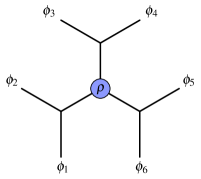
Figure 6: Snowflake OPE diagram. Here the tensor product of any two branches around the vertex $\rho$ would allow a mixed symmetry tensor of depth $\mathfrak{d}=4$ to appear in $d\geq 7$, but diagonal conformal symmetry constrains this to match with the symmetric traceless tensor produced on the third branch.

To take restrictions from the third branch $I_{3}$ into account, it is sufficient to use the total symbol of eq. (19) and impose once more our dependence statement (39) for product matrices, this time for $\mathcal{T}^{(I_{\rho,3})}$. This tells us that the matrix elements of powers

$$\left(\bar{\mathcal{T}}^{(I_{\rho,1})}+\bar{\mathcal{T}}^{(I_{\rho,2})}\right)^{n\,\,A}_{\hskip 14.0ptB}$$ (41)

with $n>2\mathfrak{d}_{3}$ can be written in terms of lower order terms. In order to convert this observation into relations among the vertex differential operators of order $p$, we can multiply the expression (41) with some appropriate powers of $\bar{\mathcal{T}}^{(I_{\rho,i})}$, $i=1,2$, and consider the matrix elements of the products

$$\left(\bar{\mathcal{T}}^{(I_{\rho,1})}+\bar{\mathcal{T}}^{(I_{\rho,2})}\right)^{n}\left(\bar{\mathcal{T}}^{(I_{\rho,2})}\right)^{\nu}\left(\bar{\mathcal{T}}^{(I_{\rho,1})}\right)^{p-n-\nu}$$ (42)

for $n>2\mathfrak{d}_{3}$, any allowed value of $p>n$ and $\nu=0,\dots,p-n$. By binomial expansion, we can write the expression (42) as a linear combination of our basic vertex differential operators. After taking relations on the branches $I_{\rho,1}$ and $I_{\rho,2}$ into account, we obtain an additional nontrivial relation from the third branch $I_{\rho,3}$. For example, in the cases where $n$ is odd, contracting (41) with $\bigl{(}\mathcal{T}^{(I_{\rho,2})}\bigr{)}^{B}_{\;\;A}$ leads to a relation between vertex and Casimir operators of order $n+1$ and further lower order operators. This effectively reduces the amount of vertex operators at order $p$ by up to $p-2\mathfrak{d}_{3}-1$, though the actual number can be lower in case there are less than $p-2\mathfrak{d}_{3}-1$ vertex operators at order $p$ left after imposing the constraints from the first two branches. If we are interested in counting the number of vertex operators at a given even order $p$, the procedure we just outlined is summarized in the following counting formula

$$n_{vdo,\rho}^{(p)}=\textit{max}\left[\left((p-2)-\sum_{i=1}^{3}\Theta_{0}(p-2\mathfrak{d}_{i})(p-2\mathfrak{d}_{i}-1)\right),0\right]\,,$$ (43)

where $\Theta_{0}$ is the Heaviside step function with $\Theta_{0}(0)=0$, the factor $(p-2)$ gives the maximal amount of vertex operators at order $p$, the factor $(p-2\mathfrak{d}_{i}-1)$ corresponds to the number of relations introduced for every $\mathfrak{d}_{i}<p/2$, and the maximum enforces the number to be $0$ if there are more than $(p-2)$ relations in total.

Our description of relations between vertex differential operators exploited the auxiliary statement (39) and did not include the Pfaffian vertex differential operators. It is clear, however, that precisely the same reasoning also applies to the latter using eq. (40) instead of eq. (39). The counting formula (43) gets also slightly modified for this Pfaffian case

$$n_{vdo,\rho}^{(p=d/2+1)}=\textit{max}\left[\left((p-2)-\sum_{i=1}^{3}\Theta_{0}(p-\mathfrak{d}_{i})(p-\mathfrak{d}_{i}-1)\right),0\right]\,.$$ (44)

Note that the arguments we have outlined here exhibit relations between vertex operators, but we have not shown that these relations are complete, i.e. that the remaining vertex differential operators are in fact independent. A priori, it could in fact happen that the exceeding relations we get from here, or additional relations obtained from a different reasoning, could provide additional dependencies. We checked however that summing the counting formulas (43) and (44) for all allowed orders $p$ in a given dimension $d$, gives rise to a number of vertex differential operators equal to the number of cross ratios (16) associated with every allowed vertex. This provides strong evidence in favor of the independence of our vertex differential operators. In some particularly relevant cases in lower dimensions we can also prove independence.

Example: The $N=6$ snowflake channel for $d=7$. Let us see how all of this works in the example of a snowflake channel in $d=7$, presented in Figure 6. We enumerate the internal links by $r=1,2,3$. The associated index sets $I_{r,i}$ are $I_{1,1}=\{1,2\},I_{2,1}=\{3,4\},\dots$. Here we have two symmetric traceless tensors associated with $r=1,2$. In a more general OPE diagram these could produce a mixed symmetry tensor with maximal depth $\mathfrak{d}=r_{d}=4$, but in the snowflake diagram the field on the third link must also be a symmetric traceless tensor of depth $\mathfrak{d}(I_{3},d=7)=2$. Our prescription tells us to consider operators (37) up to $p=8$. Eliminating powers of $\mathcal{T}_{1}=\mathcal{T}^{(12)}$ and $\mathcal{T}_{2}=\mathcal{T}^{(34)}$ higher than 4, it immediately follows that there are no vertex operators of order 8

$$\cancel{\mathcal{T}_{1}^{7}\mathcal{T}_{2}}\,,\quad\cancel{\mathcal{T}_{1}^{6}\mathcal{T}_{2}^{2}}\,,\quad\cancel{\mathcal{T}_{1}^{5}\mathcal{T}_{2}^{3}}\,,\quad\cancel{\mathcal{T}_{1}^{3}\mathcal{T}_{2}^{5}}\,,\quad\cancel{\mathcal{T}_{1}^{2}\mathcal{T}_{2}^{6}}\,,\quad\cancel{\mathcal{T}_{1}\mathcal{T}_{2}^{7}}\,,$$ (45)

while there could be up to two operators of order 6

$$\cancel{\mathcal{T}_{1}^{5}\mathcal{T}_{2}}\,,\quad\mathcal{T}_{1}^{4}\mathcal{T}_{2}^{2}\,,\quad\mathcal{T}_{1}^{2}\mathcal{T}_{2}^{4}\,,\quad\ \cancel{\mathcal{T}_{1}\mathcal{T}_{2}^{5}}\,,$$ (46)

and two operators of order 4

$$\mathcal{T}_{1}^{3}\mathcal{T}_{2}\,,\quad\mathcal{T}_{1}\mathcal{T}_{2}^{3}\,.$$ (47)

Here and in the following steps we are using notation for which stroked terms are dependent on lower order operators. Let us also recall that the operators with $\nu=p/2$ have been omitted to account for the relation between the vertex and Casimir differential operators for the third leg. The reduction of $\mathcal{T}_{3}=\mathcal{T}^{(56)}$ to a symmetric traceless tensor implies the existence of $p-2\mathfrak{d}_{3}-1$ relations between $p$ order monomials. The only useful relation in this case is the one produced for $p=6$, coming from the expansion

$$\cancel{\left(\mathcal{T}_{1}+\mathcal{T}_{2}\right)^{5}}=\mathcal{T}_{1}^{5}+5\mathcal{T}_{1}^{4}\mathcal{T}_{2}+10\mathcal{T}_{1}^{3}\mathcal{T}_{2}^{2}+10\mathcal{T}_{1}^{2}\mathcal{T}_{2}^{3}+5\mathcal{T}_{1}\mathcal{T}_{2}^{4}+\mathcal{T}_{2}^{5}\,,$$ (48)

which can be contracted with either $\mathcal{T}_{1}$ or $\mathcal{T}_{2}$ and traced over to get a relation between the sixth order monomials (including the one associated to the Casimir of the third leg):

$$\cancel{\left(\mathcal{T}_{1}+\mathcal{T}_{2}\right)^{5}\mathcal{T}_{2}}=\cancel{\mathcal{T}_{1}^{5}\mathcal{T}_{2}}+5\mathcal{T}_{1}^{4}\mathcal{T}_{2}^{2}+10\mathcal{T}_{1}^{3}\mathcal{T}_{2}^{3}+10\mathcal{T}_{1}^{2}\mathcal{T}_{2}^{4}+5\cancel{\mathcal{T}_{1}\mathcal{T}_{2}^{5}}+\cancel{\mathcal{T}_{2}^{6}}\,.$$ (49)

This reduces the amount of independent vertex operators by one, bringing us to a total of three independent operators, which matches with the number of associated cross ratios.

3 OPE channels and limits of Gaudin models

At this point we have defined a set of differential operators associated with the intermediate fields and the individual vertices of a given OPE diagram with $N$ external fields. The new vertex operators were constructed in Subsection 2.2 from a Gaudin model with three sites, which was crucial in proving their commutativity. Our construction of the vertex operators has been local in its focus on a particular building block, namely a single vertex that is associated to a local element of the OPE diagram. The purpose of this section is to adopt a more global perspective by showing that the whole set of Casimir and vertex differential operators for any $N$-point OPE channel can be obtained by taking an appropriate limit of an $N$-site Gaudin model. The $N$-site Gaudin model itself makes no reference to the choice of OPE channel. The latter enters only through the choice of limit. We will therefore refer to these limits as OPE limits of the $N$-site Gaudin model. These OPE limits are generalizations of the so-called bending flow and caterpillar limits that have been considered in the mathematical literature, see e.g. Chervov:2007dn ; Chervov:2009 ; rybnikov2016cactus . The same limit of a $4$-site Gaudin model - which may be identified with the elliptic Inozemtsev model Argyres:2021iws - has also appeared in the physics literature recently Eberhardt:2020ewh . Eberhardt, Komatsu and Mizera have shown that the limit theory coincides with the hyperbolic Calogero-Sutherland model, which is known to describe the Casimir equations of $4$-point conformal blocks.

3.1 $N$ sites Gaudin model and OPE limits

Let us first define the Gaudin model that we will use in this section. Since this construction is similar to the one of the 3-sites Gaudin model considered in Section 2.2, we refer to that section for details and references. As before, we consider a Gaudin model based on the conformal Lie algebra $\mathfrak{g}=\mathfrak{so}(d+1,1)$ but now with $N$ sites, whose positions $w_{1},\cdots,w_{N}\in\mathbb{C}$ are for the moment arbitrary. We naturally associate these sites with the $N$ external fields in the correlation function under consideration and more precisely attach to each site $i\in\{1,\cdots,N\}$ the representation of $\mathfrak{g}$ defined by the generators $\mathcal{T}_{\alpha}^{(i)}$, which describe the action of the conformal transformations on the scalar field $\phi_{i}(x_{i})$ in terms of first-order differential operators. Then we define the (components of the) Lax matrix of the model as

$$\mathcal{L}_{\alpha}(z,w_{i})=\sum_{i=1}^{N}\frac{\mathcal{T}_{\alpha}^{(i)}}{z-w_{i}}\ .$$ (50)

The associated Gaudin Hamiltonians $\mathcal{H}^{(p)}(z,w_{i})$ of degree $p$ are given by the same equation (23) that we used for the 3-site case. Recall that $\kappa_{p}$ denotes the conformally invariant symmetric tensor of degree $p$ and $\dots$ represent quantum corrections. The latter have the same form as in the 3-site case, see eq. (25). It is well known that these $N$-site Gaudin Hamiltonians commute, just as their three site analogues, i.e. they satisfy eq. (24). At the same time, it is easy to verify that they are invariant under diagonal conformal transformations,

$$\bigl{[}\mathcal{H}^{(p)}(z,w_{i}),\mathcal{T}^{(\underline{N})}_{\alpha}\bigr{]}=0,\qquad\forall\,z\in\mathbb{C},\quad\forall\,p,$$ (51)

where $\mathcal{T}^{(\underline{N})}_{\alpha}=\sum_{i=1}^{N}\mathcal{T}^{(i)}_{\alpha}$ are the diagonal conformal generators that also appear in the Ward identities (11). This means that Gaudin Hamiltonians descend to correlation functions $\mathcal{G}$.

The Hamiltonian $\mathcal{H}^{(p)}(z,w_{i})$ of the $N$-site Gaudin model depends on the $N$ complex parameters $w_{i}$ that specify the poles of the Lax matrix. These parameters have no a priori interpretation in the context of correlation functions. Note that we can always apply Möbius transformations on the $z$-variable to fix three of the $w_{i}$. This is what allowed us in the previous section to set the parameters of the 3-site Gaudin model to the specific values (27), in which case the Lax matrix (28) and its corresponding differential operators contain no extra parameters. Our main claim is that we can reconstruct the entire set of 3-site Lax matrices $\mathcal{L}^{\rho}_{\alpha}(z)$, as well as the associated vertex Hamiltonians $\mathcal{H}^{(p)}_{\rho}(z)$, one set for each vertex $\rho$, from the $N$-site Lax matrix and the associated Gaudin Hamiltonians $\mathcal{H}^{(p)}(z)=\mathcal{H}^{(p)}(z,w_{i})$ by taking appropriate scaled limits of the complex parameters $w_{i}$.

In order to make a precise statement, we need a bit of preparation. The limits we are about to discuss must depend on the choice of the OPE channel. So let us assume we are given such a channel $\mathcal{C}$. In order to define the limits we pick an (arbitrary) external edge in the diagram, which will serve as a reference point and which, up to reordering, we can suppose to have label $N$. As this edge is external, it is attached to a unique vertex, which we will denote by $\rho_{\ast}$. Such a choice of reference vertex defines a so-called rooted tree representation of the diagram. We then draw the OPE diagram on a plane, with the vertex $\rho_{\ast}$ situated at the top and with each vertex having two downward edges attached. Such a representation on a plane forces us to make a choice of which edges are pointing towards the left and which edges are pointing towards the right: this choice is arbitrary, and gives rise to what is called a plane (or ordered) representation of the underlying rooted tree. We give an example of such a plane rooted tree representation for an 8-point OPE diagram in Figure 7 below.

Figure 7: Plane rooted tree representation of an OPE diagram with 8 external fields.

Recall from Section 1 that each vertex $\rho$ of the OPE diagram defines a partition $\underline{N}=I_{\rho,1}\mathbin{\mathchoice{\leavevmode\vtop{\halign{\hfil$\m@th\displaystyle#$\hfil\cr\cup\cr\cdot\crcr}}}{\leavevmode\vtop{\halign{\hfil$\m@th\textstyle#$\hfil\cr\cup\cr\cdot\crcr}}}{\leavevmode\vtop{\halign{\hfil$\m@th\scriptstyle#$\hfil\cr\cup\cr\cdot\crcr}}}{\leavevmode\vtop{\halign{\hfil$\m@th\scriptscriptstyle#$\hfil\cr\cup\cr\cdot\crcr}}}}I_{\rho,2}\mathbin{\mathchoice{\leavevmode\vtop{\halign{\hfil$\m@th\displaystyle#$\hfil\cr\cup\cr\cdot\crcr}}}{\leavevmode\vtop{\halign{\hfil$\m@th\textstyle#$\hfil\cr\cup\cr\cdot\crcr}}}{\leavevmode\vtop{\halign{\hfil$\m@th\scriptstyle#$\hfil\cr\cup\cr\cdot\crcr}}}{\leavevmode\vtop{\halign{\hfil$\m@th\scriptscriptstyle#$\hfil\cr\cup\cr\cdot\crcr}}}}I_{\rho,3}$, with the sets $I_{\rho,j}$ formed by the labels of the external fields attached to the three branches of the vertex. Although the choice of labeling of these branches was arbitrary in Section 1, we will now fix it using the plane rooted tree representation of the diagram picked above: choose the branch $I_{\rho,1}$ to be the one pointing to the bottom left and the branch $I_{\rho,2}$ to be the one pointing to the bottom right. By construction, the last branch $I_{\rho,3}$ then always points to the top and contains the reference point $N$.

Each vertex $\rho$ in the diagram is thereby associated with a sequence $s^{\rho}=(s^{\rho}_{1},s^{\rho}_{2},\dots,s^{\rho}_{n_{\rho}})$ of elements $s^{\rho}_{a}\in\{1,2\}$. This sequence $s^{\rho}$ encodes the path from $\rho_{\ast}$ to $\rho$. It tells us whether we have to move to the left (for $s_{a}^{\rho}=1$) or right (for $s_{a}^{\rho}=2$) every time we reach a new vertex until we arrive at $\rho$ after $n_{\rho}$ steps. We shall also refer to the length $n_{\rho}$ of the sequence as the depth of the vertex and to $s^{\rho}$ as the binary sequence of $\rho$. Note that the top vertex $\rho_{\ast}$ has depth $n_{\rho_{\ast}}=0$. Let us point out that the notion of depth used in this section refers to the distance from the root $\rho_{\ast}$ and is very different from the depth $\mathfrak{d}$ introduced in eq. (12) of the introduction.

In order to construct the limit of the Gaudin model that we are interested in, we will need to assign a polynomial $g_{\rho}(\varpi)$ to each vertex $\rho$. If $s^{\rho}$ is the binary sequence associated with the vertex $\rho$, the polynomial $g_{\rho}$ is defined as

$$g_{\rho}(\varpi)=\sum_{a=1}^{n_{\rho}}\varpi^{a-1}\delta_{s_{a}^{\rho},2}\ .$$ (52)

Obviously the top vertex $\rho_{\ast}$ is assigned to $g_{\rho_{\ast}}(\varpi)=0$. The vertices of depth $n_{\rho}=1$ are associated with $g_{\rho_{1}}(\varpi)=0$ or $g_{\rho_{2}}(\varpi)=1$, depending on whether they are reached from $\rho_{\ast}$ by going down to the left ($\rho_{1}$) or to the right ($\rho_{2}$).

Similarly, we can assign polynomials $f_{i}(\varpi)$ to each external edge $1\leq i<N$ at the bottom of the plane rooted tree. Once again, we can encode the path from $\rho_{\ast}$ down to the edge $i$ by a binary sequence $s^{i}=(s^{i}_{1},s^{i}_{2},\dots,s_{n_{i}}^{i})$. The length $n_{i}$ of the sequence $s^{i}$ is also referred to as the depth of the edge $i$. Now we introduce

$$f_{i}(\varpi)=\sum_{a=1}^{n_{i}}\varpi^{a-1}\delta_{s^{i}_{a},2}+\varpi^{n_{i}}\delta_{s^{i}_{n_{i}},1}\ .$$ (53)

and set

$$f_{N}(\varpi)=\varpi^{-1}$$ (54)

for the external edge of the reference field at the top of the plane rooted tree. Thereby we have now set up all the necessary notation that is needed to construct the relevant scaling limits of the $N$-site Gaudin model.

We can now move on to the main result of this section, namely how to reconstruct the vertex Hamiltonians $\mathcal{H}^{(p)}_{\rho}(z)$ of the 3-site Gaudin model of the previous section from the $N$-site Hamiltonians $\mathcal{H}^{(p)}(z)=\mathcal{H}^{(p)}(z,w_{i})$. To this end, we will first construct the vertex Lax matrices (28) from the Lax matrix (50) before studying the associated Hamiltonians (23) in the limit. As it turns out, we can recover the parameter free Lax matrix $\mathcal{L}^{\rho}$ that is associated with the vertex $\rho$ as

$$\mathcal{L}_{\alpha}^{\rho}(z)=\frac{\mathcal{T}_{\alpha}^{(I_{\rho,1})}}{z}+\frac{\mathcal{T}_{\alpha}^{(I_{\rho,2})}}{z-1}=\lim_{\varpi\to 0}\ \varpi^{n_{\rho}}\mathcal{L}_{\alpha}\bigl{(}\varpi^{n_{\rho}}z+g_{\rho}(\varpi),w_{i}=f_{i}(\varpi)\bigr{)}\ .$$ (55)

Let us note that in the limit, the site $w_{N}=\varpi^{-1}$ associated with the reference field $N$ goes to infinity, while the sites of the other external fields approach $z=0$ or $z=1$ depending on whether they are located at the right or left branch of the the plane rooted tree, i.e. whether their binary sequence $s^{\rho}$ starts with $s^{\rho}_{1}=1$ or $s^{\rho}_{1}=2$. We shall prove eq. (55) in the third Subsection 3.3 through a recursive procedure that will also offer insight into the construction of the polynomials $g_{\rho}$ and $f_{i}$.

Let us now turn to the limit construction for the Gaudin Hamiltonians. We claim that the Hamiltonians $\mathcal{H}^{(p)}(z,w_{i})$ of the $N$-sites Gaudin model give rise to the Hamiltonians $\mathcal{H}^{(p)}_{\rho}(z)$ of the different 3-sites vertex Gaudin models defined in Section 2.2 as

$$\mathcal{H}_{\rho}^{(p)}(z)=\lim_{\varpi\to 0}\varpi^{pn_{\rho}}\mathcal{H}^{(p)}\bigl{(}\varpi^{n_{\rho}}z+g_{\rho}(\varpi),w_{i}=f_{i}(\varpi)\bigr{)}\ .$$ (56)

The fact that this statement holds for the leading part of the Hamiltonians, without quantum corrections, follows directly from the corresponding limit (55) of the Lax matrix

$$\varpi^{pn_{\rho}}\kappa_{p}^{\alpha_{1}\cdots\alpha_{p}}\mathcal{L}_{\alpha_{1}}\bigl{(}\varpi^{n_{\rho}}z+g_{\rho}(\varpi)\bigr{)}\cdots\mathcal{L}_{\alpha_{p}}\bigl{(}\varpi^{n_{\rho}}z+g_{\rho}(\varpi)\bigr{)}\xrightarrow{\varpi\to 0}\kappa^{\alpha_{1}\cdots\alpha_{p}}\mathcal{L}_{\alpha_{1}}^{\rho}(z)\cdots\mathcal{L}_{\alpha_{p}}^{\rho}(z)\ .$$

But it requires a bit of work to argue that the quantum corrections also have the required behaviour under the limit. Consider a term of the form (25) in the correction: by appropriately distributing the powers $\varpi^{pn_{\rho}}$, using the fact that $r_{1}+\cdots+r_{q}=p$, and performing the change of spectral parameter $z\mapsto z^{\prime}_{\rho}(\varpi)=\varpi^{n_{\rho}}z+g_{\rho}(\varpi)$ in the derivatives, we find that

$$\varpi^{pn_{\rho}}\tau^{\alpha_{1}\cdots\alpha_{q}}\;\partial_{z^{\prime}_{\rho}(\varpi)}^{r_{1}-1}\mathcal{L}_{\alpha_{1}}\bigl{(}z^{\prime}_{\rho}(\varpi)\bigr{)}\cdots\partial_{z^{\prime}_{\rho}(\varpi)}^{r_{q}-1}\mathcal{L}_{\alpha_{q}}\bigl{(}z^{\prime}_{\rho}(\varpi)\bigr{)}$$

$$\hskip 15.0pt=\hskip 15.0pt\tau^{\alpha_{1}\cdots\alpha_{q}}\partial^{r_{1}-1}_{z}\Bigl{(}\omega^{n_{\rho}}\mathcal{L}_{\alpha_{1}}\bigl{(}\varpi^{n_{\rho}}z+g_{\rho}(\varpi)\bigr{)}\Bigr{)}\cdots\partial^{r_{q}-1}_{z}\Bigl{(}\omega^{n_{\rho}}\mathcal{L}_{\alpha_{q}}\bigl{(}\varpi^{n_{\rho}}z+g_{\rho}(\varpi)\bigr{)}\Bigr{)}$$

$$\hskip 7.0pt\xrightarrow{\varpi\to 0}\hskip 7.0pt\tau^{\alpha_{1}\cdots\alpha_{q}}\;\partial_{z}^{r_{1}-1}\mathcal{L}^{\rho}_{\alpha_{1}}(z)\cdots\partial_{z}^{r_{q}-1}\mathcal{L}^{\rho}_{\alpha_{q}}(z),$$

such that this correction term reduces in the OPE limit to the corresponding correction in $\mathcal{H}_{\rho}^{(p)}(z)$.

As the vertex operators $\mathcal{D}_{\rho}^{p,\nu}$ and the Casimir operators $\mathcal{D}_{r}^{p}$ of the intermediate fields attached to the vertex $\rho$ are naturally extracted from the Hamiltonian $\mathcal{H}^{(p)}_{\rho}(z)$, the property (56) shows that the full set of operators defined in Section 1 can be obtained from the limit of the $N$-sites Gaudin model considered here. Before the limit $\varpi\to 0$, The commutativity property (24) of the $N$-site Gaudin Hamiltonians can be written as

$$\Bigl{[}\mathcal{H}^{(p)}\bigl{(}\varpi^{n_{\rho}}z+g_{\rho}(\varpi)\bigr{)},\mathcal{H}^{(q)}\bigl{(}\varpi^{n_{\rho}}w+g_{\rho}(\varpi)\bigr{)}\Bigr{]}=0,\qquad\forall\,z,w\in\mathbb{C},\quad\forall\,p,q,\quad\forall\,\rho,\rho^{\prime}.$$ (57)

for arbitrary $\varpi$, and is therefore preserved in the limit $\varpi\to 0$,

$$\bigl{[}\mathcal{H}^{(p)}_{\rho}(z),\mathcal{H}^{(q)}_{\rho^{\prime}}(w)\bigr{]}=0,\qquad\forall\,z,w\in\mathbb{C},\quad\forall\,p,q,\quad\forall\,\rho,\rho^{\prime}.$$ (58)

This provides an alternative proof of the commutativity of all Casimir operators $\mathcal{D}_{r}^{p}$ and vertex operators $\mathcal{D}_{\rho}^{p,\nu}$. Moreover, this statement now holds without needing to use conformal Ward identities. The proof relies on a specific choice of labeling of the edges at vertices, given by a plane rooted tree representation of the OPE diagram. Different such representations of the diagram correspond to different limits of the same underlying $N$-sites Gaudin model and give rise to different sets of commuting operators, which however generate the same algebra when acting on solutions of the conformal Ward identities. Finally, let us note that the above construction automatically ensures the compatibility of these operators with the conformal Ward identities, since taking appropriate limits of eq. (51) demonstrates that they commute with the diagonal conformal generators $\mathcal{T}_{\alpha}^{(\underline{N})}$.

3.2 Examples

Before we prove our main result, let us illustrate the construction of the operators from limits of Gaudin models with two examples. The first one addresses the so-called comb channel OPE diagrams for which we have already outlined the limit in Buric:2020dyz . The second example deals with the snowflake OPE channel of the $N=6$-point function.

Comb channel.

Let us consider the comb channel OPE diagram with $N$ external fields. To apply the construction of the present section, we first need to pick a plane rooted tree representation of this diagram. We will choose to represent it with all internal edges pointing towards the bottom left. We then label the external edges of the tree as follows: we let $N$ be the top edge of the tree, $1$ be edge furthest to the left and label by $2,\cdots,N-1$ the external edges pointing to the bottom right at each vertex, from the bottom to the top. Moreover, following our conventions in Buric:2020dyz , we enumerate the vertices $\rho=[r]$ by an integer $r=1,\dots,N-2$, from bottom to top. We represent this plane rooted tree in Figure 8 below, with external edges indicated in black and vertices in blue.

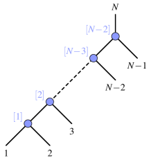
Figure 8: Choice of plane rooted tree representation of the comb channel OPE diagram with $N$ points.

One can compute the limit of the Gaudin model associated with this tree using the construction outlined in the previous subsection. For the polynomials $f_{i}$ that determine the parameters $w_{i}$ of the Gaudin model, one finds from eq. (53) that

$$w_{i}=f_{i}(\varpi)=\varpi^{N-1-i},\qquad\forall\,i\in\{1,\cdots,N\}\ .$$ (59)

Let us now consider the vertices $\rho=[r]$, with $r=1,\dots,N-2$. From the general construction, and formula (52) in particular, we find

$$n_{[r]}=N-2-r\qquad\text{ and }\qquad g_{[r]}(\varpi)=0,\qquad\forall\,r\in\{1,\cdots,N-2\}\ .$$ (60)

Note in particular that for this choice of plane rooted tree, the polynomial functions $g_{\rho}$ are all zero, since all vertices $\rho=[r]$ sit on the most left branch of the tree. The limit of the Gaudin Lax matrix

$$\mathcal{L}_{\alpha}(z,w_{i}=f_{i}(\varpi))=\sum_{i=1}^{N}\frac{\mathcal{T}^{(i)}_{\alpha}}{z-\varpi^{N-1-i}}$$ (61)

associated with the vertex $[r]$ then reads

$$\varpi^{N-2-r}\mathcal{L}_{\alpha}\bigl{(}\varpi^{N-2-r}z\bigr{)}\xrightarrow{\varpi\to 0}\mathcal{L}_{\alpha}^{[r]}(z)=\frac{\mathcal{T}_{\alpha}^{(1)}+\cdots+\mathcal{T}_{\alpha}^{(r)}}{z}+\frac{\mathcal{T}^{(r+1)}}{z-1}.$$ (62)

In sum, the vertex Gaudin Hamiltonians of the comb channel OPE limit are

$$\varpi^{p(N-2-r)}\mathcal{H}^{(p)}\bigl{(}\varpi^{N-2-r}z\bigr{)}\xrightarrow{\varpi\to 0}\mathcal{H}_{[r]}^{(p)}(z).$$ (63)

The above limit coincides exactly with the one introduced in Buric:2020dyz to describe the comb channel, thus showing that the results of Buric:2020dyz are contained in the more general construction discussed here.

Snowflake channel.

The results of the present article allow us to discuss more general topologies of OPE diagrams than the comb channel. The first example of such a topology is the snowflake channel of $6$-point functions. We represent this OPE diagram as a plane rooted tree following the conventions of Figure 9, where the external edges are labeled in black from $1$ to $6$ and the vertices are labeled in blue from $[1]$ to $[4]$. Note in particular that the internal vertex of the diagram corresponds here to the label $[3]$.

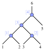
Figure 9: Choice of plane rooted tree representation of the snowflake OPE diagram.

We can immediately read off the depth of the four vertices as

$$n_{[1]}=n_{[2]}=2,\qquad n_{[3]}=1,\qquad n_{[4]}=0.$$ (64)

We can now encode the positions of all four vertices in a binary sequence and apply the formulas (52) to construct the polynomials $g_{\rho}$, yielding

$$g_{[1]}(\varpi)=g_{[3]}(\varpi)=g_{[4]}(\varpi)=0\qquad\text{ and }\qquad g_{[2]}(\varpi)=\varpi.$$ (65)

Similarly, one can encode the five external edges at the bottom of the diagram in binary sequences and apply eq. (53) to determine the positions of the $N=6$ sites,

$$w_{1}=\varpi^{3},\qquad w_{2}=\varpi^{2},\qquad w_{3}=\varpi+\varpi^{3},\qquad w_{4}=\varpi+\varpi^{2},\qquad w_{5}=1,\qquad w_{6}=\frac{1}{\varpi}.$$ (66)

Inserting this parameterization of the complex parameters $w_{i}$ in terms of $\varpi$ back into the Lax matrix of the 6-sites Gaudin model, we obtain

$$\mathcal{L}_{\alpha}(z)=\frac{\mathcal{T}_{\alpha}^{(1)}}{z-\varpi^{3}}+\frac{\mathcal{T}_{\alpha}^{(2)}}{z-\varpi^{2}}+\frac{\mathcal{T}_{\alpha}^{(3)}}{z-\varpi-\varpi^{3}}+\frac{\mathcal{T}_{\alpha}^{(4)}}{z-\varpi-\varpi^{2}}+\frac{\mathcal{T}_{\alpha}^{(5)}}{z-1}+\frac{\varpi\,\mathcal{T}_{\alpha}^{(6)}}{\varpi\,z-1}.$$ (67)

Given this expression and our formulas for $n_{\rho}$ and $g_{\rho}$, it is now straightforward to check the limits (55) for all four vertices,

$$\varpi^{2}\mathcal{L}_{\alpha}(\varpi^{2}z)\xrightarrow{\varpi\to 0}\frac{\mathcal{T}_{\alpha}^{(1)}}{z}+\frac{\mathcal{T}_{\alpha}^{(2)}}{z-1},\qquad\varpi^{2}\mathcal{L}_{\alpha}(\varpi^{2}z+\varpi)\xrightarrow{\varpi\to 0}\frac{\mathcal{T}_{\alpha}^{(3)}}{z}+\frac{\mathcal{T}_{\alpha}^{(4)}}{z-1},$$ (68)

$$\varpi\mathcal{L}_{\alpha}(\varpi z)\xrightarrow{\varpi\to 0}\frac{\mathcal{T}_{\alpha}^{(1)}+\mathcal{T}_{\alpha}^{(2)}}{z}+\frac{\mathcal{T}_{\alpha}^{(3)}+\mathcal{T}_{\alpha}^{(4)}}{z-1},\qquad\mathcal{L}_{\alpha}(z)\xrightarrow{\varpi\to 0}\frac{\mathcal{T}_{\alpha}^{(1)}+\mathcal{T}_{\alpha}^{(2)}+\mathcal{T}_{\alpha}^{(3)}+\mathcal{T}_{\alpha}^{(4)}}{z}+\frac{\mathcal{T}_{\alpha}^{(5)}}{z-1}.$$

These indeed give the expected vertex Lax matrices $\mathcal{L}_{\alpha}^{\rho}=\mathcal{L}_{\alpha}^{[r]}$ for the vertices labeled by $r=1,2,3,4$. These two examples suffice to gain a first intuition into how we take limits of Gaudin models and thereby manage to embed the vertex Lax matrices into the full $N$-sites model. We will now explain the derivation of our results for general OPE diagrams.

3.3 Recursive proof of the limits

Subtrees.

Our goal in this subsection is to prove that our limit construction is indeed able to recover all vertex Lax matrices, as we have claimed. Let us consider some OPE channel $\mathcal{C}$ represented by a plane rooted tree $T$. The approach that we follow is recursive. Let us consider the top vertex $\rho_{\ast}$ of the tree, which is by construction attached to the external edge $N$. We denote by $e^{\prime}$ and $e^{\prime\prime}$ the left and right downward edges attached to $\rho_{\ast}$ (which can correspond to either external or intermediate fields depending on the topology of the diagram). We can then see the tree $T$ as being composed of the vertex $\rho_{\ast}$ and of two (plane rooted) subtrees with reference edges $e^{\prime}$ and $e^{\prime\prime}$, which we will call $T^{\prime}$ and $T^{\prime\prime}$ respectively. In Figure 10 below, we illustrate the two subtrees obtained in the example of Figure 7.

Figure 10: Subtrees of the tree 7.

We will now prove that if the limit construction of Subsection 3.1 holds for the subtrees $T^{\prime}$ and $T^{\prime\prime}$, then it also holds for the initial tree $T$, thus proving that it holds for any tree by induction. Let us first introduce some useful notation. We will denote by $E^{\prime}$ and $E^{\prime\prime}$ the external edges of $T$ that belong to the subtrees $T^{\prime}$ and $T^{\prime\prime}$ respectively. Note that if $T^{\prime}$ is not trivial, i.e. if $e^{\prime}$ is not an external edge of the initial tree $T$, then the full set of external edges of $T^{\prime}$ is $E^{\prime}\mathbin{\mathchoice{\leavevmode\vtop{\halign{\hfil$\m@th\displaystyle#$\hfil\cr\cup\cr\cdot\crcr}}}{\leavevmode\vtop{\halign{\hfil$\m@th\textstyle#$\hfil\cr\cup\cr\cdot\crcr}}}{\leavevmode\vtop{\halign{\hfil$\m@th\scriptstyle#$\hfil\cr\cup\cr\cdot\crcr}}}{\leavevmode\vtop{\halign{\hfil$\m@th\scriptscriptstyle#$\hfil\cr\cup\cr\cdot\crcr}}}}\{e^{\prime}\}$ (since $e^{\prime}$ is external in $T^{\prime}$ but not in $T$). On the other hand, if $e^{\prime}$ is external in $T$, then we simply have $E^{\prime}=\{e^{\prime}\}$ and the subtree $T^{\prime}$ is trivial. Let us also denote by $V$, $V^{\prime}$ and $V^{\prime\prime}$ the set of vertices of $T$, $T^{\prime}$ and $T^{\prime\prime}$, such that $V=V^{\prime}\mathbin{\mathchoice{\leavevmode\vtop{\halign{\hfil$\m@th\displaystyle#$\hfil\cr\cup\cr\cdot\crcr}}}{\leavevmode\vtop{\halign{\hfil$\m@th\textstyle#$\hfil\cr\cup\cr\cdot\crcr}}}{\leavevmode\vtop{\halign{\hfil$\m@th\scriptstyle#$\hfil\cr\cup\cr\cdot\crcr}}}{\leavevmode\vtop{\halign{\hfil$\m@th\scriptscriptstyle#$\hfil\cr\cup\cr\cdot\crcr}}}}V^{\prime\prime}\mathbin{\mathchoice{\leavevmode\vtop{\halign{\hfil$\m@th\displaystyle#$\hfil\cr\cup\cr\cdot\crcr}}}{\leavevmode\vtop{\halign{\hfil$\m@th\textstyle#$\hfil\cr\cup\cr\cdot\crcr}}}{\leavevmode\vtop{\halign{\hfil$\m@th\scriptstyle#$\hfil\cr\cup\cr\cdot\crcr}}}{\leavevmode\vtop{\halign{\hfil$\m@th\scriptscriptstyle#$\hfil\cr\cup\cr\cdot\crcr}}}}\{\rho_{\ast}\}$.

Recursion relations.

Recall the polynomial $g_{\rho}(\varpi)$ defined in eq. (52) for any vertex $\rho\in V$ of $T$ in terms of the binary sequence $s^{\rho}=(s^{\rho}_{1},\cdots,s^{\rho}_{n_{\rho}})$. Let us suppose that this vertex is contained in the subtree $T^{\prime}$ and thus belongs to $V^{\prime}$: it is then associated with a binary sequence $s^{\prime\,\rho}=(s^{\prime\,\rho}_{1},\cdots,s^{\prime\,\rho}_{n^{\prime}_{\rho}})$ in $T^{\prime}$. By construction, the depth $n^{\prime}_{\rho}$ of $\rho$ in $T^{\prime}$ is given by $n_{\rho}-1$. Moreover, it is clear that the binary sequence of $\rho$ in $T$ is related to that in $T^{\prime}$ by $s^{\rho}=(1,s^{\prime\,\rho}_{1},\cdots,s^{\prime\,\rho}_{n_{\rho}-1})$. Indeed, since $\rho$ belongs to $T^{\prime}$, the path from $\rho_{\ast}$ to $\rho$ starts by going to the bottom left ($s^{\rho}_{1}=1$), and is then given by the path from $e^{\prime}$ to $\rho$, encoded by $s^{\prime\,\rho}$. It is then clear that the polynomial $g_{\rho}(\varpi)$ defined by eq. (52) is related to the corresponding polynomial $g^{\prime}_{\rho}(\varpi)$ defined for $T^{\prime}$ by $g_{\rho}(\varpi)=\varpi\,g^{\prime}_{\rho}(\varpi)$. Similarly, if $\rho$ belongs to $V^{\prime\prime}$, we have $s^{\rho}=(2,s^{\prime\prime\,\rho}_{1},\cdots,s^{\prime\prime\,\rho}_{n_{\rho}-1})$ and thus $g_{\rho}(\varpi)=1+\varpi\,g^{\prime\prime}_{\rho}(\varpi)$. In conclusion, the polynomials $g_{\rho}(\varpi)$ satisfy the recursion relation

$$g_{\rho}(\varpi)=\left\{\begin{array}[]{ll}\varpi g^{\prime}_{\rho}(\varpi)&\text{ if }\rho\in V^{\prime},\\ 1+\varpi g^{\prime\prime}_{\rho}(\varpi)&\text{ if }\rho\in V^{\prime\prime},\\ 0&\text{ if }\rho=\rho_{\ast}.\end{array}\right.$$ (69)

A similar analysis can be performed for the sites $w_{i}=f_{i}(\varpi)$ associated with the external edges $i\in\underline{N}$ through eq. (53), distinguishing three cases. If $i=N$ is the top reference edge, then we recall that $w_{N}=f_{N}(\varpi)=\varpi^{-1}$. If $i\in E^{\prime}$ is an edge belonging to the subtree $T^{\prime}$, then one can relate the binary sequences $s^{i}$ and $s^{\prime\,i}$ describing $i$ in $T$ and $T^{\prime}$ in a similar way as for the vertices in the paragraph above. We then find that the polynomial $f_{i}(\varpi)$ satisfy the recursion relation

$$f_{i}(\varpi)=\left\{\begin{array}[]{ll}\varpi&\text{ if }e^{\prime}\text{ is external in }T,\\ \varpi f^{\prime}_{i}(\varpi)&\text{ else.}\end{array}\right.$$ (70)

Note that in the first case, the subtree $T^{\prime}$ is trivial and the index $i$ is then necessarily equal to $e^{\prime}$, while in the second case $i$ is different from $e^{\prime}$ and the subtree $T^{\prime}$ is therefore non-trivial. Finally, if $i\in E^{\prime\prime}$ belongs to the subtree $T^{\prime\prime}$, then we similarly find

$$f_{i}(\varpi)=\left\{\begin{array}[]{ll}1&\text{ if }e^{\prime\prime}\text{ is external in }T,\\ 1+\varpi f^{\prime\prime}_{i}(\varpi)&\text{ else.}\end{array}\right.$$ (71)

Here, $i=e^{\prime\prime}$ in the first case and $i\neq e^{\prime\prime}$ in the second one.

Induction hypotheses.

We will now suppose that the limit procedure defined in Subsection 3.1 holds for the subtrees $T^{\prime}$ and $T^{\prime\prime}$. To phrase these induction hypotheses more precisely, let us focus first on the subtree $T^{\prime}$. If it is non-trivial, i.e. if $e^{\prime}$ is not external in $T$, the external edges of $T^{\prime}$ are $E^{\prime}\mathbin{\mathchoice{\leavevmode\vtop{\halign{\hfil$\m@th\displaystyle#$\hfil\cr\cup\cr\cdot\crcr}}}{\leavevmode\vtop{\halign{\hfil$\m@th\textstyle#$\hfil\cr\cup\cr\cdot\crcr}}}{\leavevmode\vtop{\halign{\hfil$\m@th\scriptstyle#$\hfil\cr\cup\cr\cdot\crcr}}}{\leavevmode\vtop{\halign{\hfil$\m@th\scriptscriptstyle#$\hfil\cr\cup\cr\cdot\crcr}}}}\{e^{\prime}\}$. We then introduce the Gaudin Lax matrix associated with $T^{\prime}$ as

$$\mathcal{L}^{\prime}_{\alpha}(z)=\sum_{i\in E^{\prime}\mathbin{\mathchoice{\leavevmode\vtop{\halign{\hfil$\m@th\displaystyle#$\hfil\cr\cup\cr\cdot\crcr}}}{\leavevmode\vtop{\halign{\hfil$\m@th\textstyle#$\hfil\cr\cup\cr\cdot\crcr}}}{\leavevmode\vtop{\halign{\hfil$\m@th\scriptstyle#$\hfil\cr\cup\cr\cdot\crcr}}}{\leavevmode\vtop{\halign{\hfil$\m@th\scriptscriptstyle#$\hfil\cr\cup\cr\cdot\crcr}}}}\{e^{\prime}\}}\frac{\mathcal{T}_{\alpha}^{(i)}}{z-f^{\prime}_{i}(\varpi)},$$ (72)

where the sites associated with the external edges $E^{\prime}\mathbin{\mathchoice{\leavevmode\vtop{\halign{\hfil$\m@th\displaystyle#$\hfil\cr\cup\cr\cdot\crcr}}}{\leavevmode\vtop{\halign{\hfil$\m@th\textstyle#$\hfil\cr\cup\cr\cdot\crcr}}}{\leavevmode\vtop{\halign{\hfil$\m@th\scriptstyle#$\hfil\cr\cup\cr\cdot\crcr}}}{\leavevmode\vtop{\halign{\hfil$\m@th\scriptscriptstyle#$\hfil\cr\cup\cr\cdot\crcr}}}}\{e^{\prime}\}$ are set to the positions $f^{\prime}_{i}(\varpi)$ prescribed by the limit procedure of Subsection 3.1. Here, the generators $\mathcal{T}_{\alpha}^{(i)}$ associated with external fields $i\in E^{\prime}$ are defined by their expression in the initial tree $T$, while the generators associated with $e^{\prime}$ are defined by $\mathcal{T}_{\alpha}^{(e^{\prime})}=\mathcal{T}_{\alpha}^{(\underline{N}\setminus E^{\prime})}$. By construction, the latter satisfy the commutation relations of $\mathfrak{g}$ and commute with the other generators $\mathcal{T}_{\alpha}^{(i)}$, $i\in E^{\prime}$, as required. Moreover, this definition ensures that the diagonal conformal generators $\sum_{i\in\underline{N}}\mathcal{T}_{\alpha}^{(i)}$ of the tree $T$ coincides with the ones $\sum_{i\in E^{\prime}\mathbin{\mathchoice{\leavevmode\vtop{\halign{\hfil$\m@th\displaystyle#$\hfil\cr\cup\cr\cdot\crcr}}}{\leavevmode\vtop{\halign{\hfil$\m@th\textstyle#$\hfil\cr\cup\cr\cdot\crcr}}}{\leavevmode\vtop{\halign{\hfil$\m@th\scriptstyle#$\hfil\cr\cup\cr\cdot\crcr}}}{\leavevmode\vtop{\halign{\hfil$\m@th\scriptscriptstyle#$\hfil\cr\cup\cr\cdot\crcr}}}}\{e^{\prime}\}}\mathcal{T}_{\alpha}^{(i)}$ of $T^{\prime}$ (however, as we will see, the definition of $\mathcal{T}_{\alpha}^{(e^{\prime})}$ is in fact irrelevant for the recursive proof).

As $T^{\prime}$ is assumed to be non-trivial here, its vertex set $V^{\prime}$ is non-empty. The induction hypothesis that we make in this subsection is then that eq. (55) holds for the subtree $T^{\prime}$, that is to say

$$\mathcal{L}_{\alpha}^{\rho}(z)=\frac{\mathcal{T}_{\alpha}^{(I_{\rho,1})}}{z}+\frac{\mathcal{T}_{\alpha}^{(I_{\rho,2})}}{z-1}=\lim_{\varpi\to 0}\ \varpi^{n^{\prime}_{\rho}}\mathcal{L}^{\prime}_{\alpha}\bigl{(}\varpi^{n^{\prime}_{\rho}}z+g^{\prime}_{\rho}(\varpi)\bigr{)},\qquad\forall\rho\in V^{\prime}.$$ (73)

In this equation, we used the Lax matrix $\mathcal{L}_{\alpha}^{\rho}(z)$ associated with the vertex $\rho$ as defined in the initial tree $T$: indeed, it is clear that this vertex Lax matrix coincides with the one associated with $\rho$ in the subtree $T^{\prime}$ (in particular, the subsets of external edges $I_{\rho,1}$ and $I_{\rho,2}$ associated with the left and right branches of $\rho$ are the same when defined for $T$ as when defined for $T^{\prime}$).

Similarly, if $T^{\prime\prime}$ is non-trivial, we consider the associated Lax matrix

$$\mathcal{L}^{\prime\prime}_{\alpha}(z)=\sum_{i\in E^{\prime\prime}\mathbin{\mathchoice{\leavevmode\vtop{\halign{\hfil$\m@th\displaystyle#$\hfil\cr\cup\cr\cdot\crcr}}}{\leavevmode\vtop{\halign{\hfil$\m@th\textstyle#$\hfil\cr\cup\cr\cdot\crcr}}}{\leavevmode\vtop{\halign{\hfil$\m@th\scriptstyle#$\hfil\cr\cup\cr\cdot\crcr}}}{\leavevmode\vtop{\halign{\hfil$\m@th\scriptscriptstyle#$\hfil\cr\cup\cr\cdot\crcr}}}}\{e^{\prime\prime}\}}\frac{\mathcal{T}_{\alpha}^{(i)}}{z-f^{\prime\prime}_{i}(\varpi)},$$ (74)

and suppose that it satisfies the induction hypothesis

$$\mathcal{L}_{\alpha}^{\rho}(z)=\frac{\mathcal{T}_{\alpha}^{(I_{\rho,1})}}{z}+\frac{\mathcal{T}_{\alpha}^{(I_{\rho,2})}}{z-1}=\lim_{\varpi\to 0}\ \varpi^{n^{\prime\prime}_{\rho}}\mathcal{L}^{\prime\prime}_{\alpha}\bigl{(}\varpi^{n^{\prime\prime}_{\rho}}z+g^{\prime\prime}_{\rho}(\varpi)\bigr{)},\qquad\forall\rho\in V^{\prime\prime}.$$ (75)

Proof of the induction.

We are now in a position to prove that the induction carries from the subtrees $T^{\prime}$ and $T^{\prime\prime}$ to $T$. For that, we will show that the limit (55) holds for every vertex $\rho\in V$, with three cases to distinguish. If $\rho\in V^{\prime}$ belongs to the subtree $T^{\prime}$, we will use the induction hypothesis (73) and the recursion relations (69), first case, and (70). Similarly, if $\rho\in V^{\prime\prime}$ belongs to $T^{\prime\prime}$, we will use the induction hypothesis (75) and the recursion relations (69), second case, and (71). Finally, if $\rho$ is the reference vertex $\rho_{\ast}$, then the limit will follow without having to use any induction hypothesis. As these proofs are rather technical, we gather them in Appendix A.

4 Example: 5-point conformal blocks

As an example of our construction of commuting differential operators, let us consider a correlator of five scalar fields

$$\expectationvalue{\phi_{1}\phi_{2}\phi_{3}\phi_{4}\phi_{5}}$$ (76)

and fix the OPE decomposition as in Figure 2.

This correlator can be be written schematically as

$$\expectationvalue{\phi_{1}\phi_{2}\phi_{3}\phi_{4}\phi_{5}}=\Omega^{(\Delta_{i})}_{5}(x_{i})\psi^{(\Delta_{i})}(u_{1},\dots,u_{5})$$ (77)

where $\Omega^{(\Delta_{i})}_{5}(x_{i})$ is a prefactor that takes into account the covariance of the correlator with respect to conformal transformations, while $\psi^{(\Delta_{i})}(u_{1},\dots,u_{5})$ is a conformally invariant function which depends on five cross ratios and admits a conformal block decomposition. In order to obtain differential equations for 5-point conformal blocks, one first needs to determine which Casimir and vertex operators characterize these blocks, and then compute their action on the space of cross ratios $u_{i}$.

For the OPE decomposition of Figure 2, the recipe of Section 2 instructs us to construct four Casimir operators, two for each internal leg

$$\mathcal{D}^{2}_{(12)}= \left(\mathcal{T}_{1}+\mathcal{T}_{2}\right)_{[AB]}\left(\mathcal{T}_{1}+\mathcal{T}_{2}\right)^{[BA]}\,,$$ (78)

$$\mathcal{D}^{2}_{(45)}= \left(\mathcal{T}_{4}+\mathcal{T}_{5}\right)_{[AB]}\left(\mathcal{T}_{4}+\mathcal{T}_{5}\right)^{[BA]}\,,$$ (79)

$$\mathcal{D}^{4}_{(12)}= \left(\mathcal{T}_{1}+\mathcal{T}_{2}\right)_{[AB]}\left(\mathcal{T}_{1}+\mathcal{T}_{2}\right)^{[BC]}\left(\mathcal{T}_{1}+\mathcal{T}_{2}\right)_{[CD]}\left(\mathcal{T}_{1}+\mathcal{T}_{2}\right)^{[DA]}\,,$$ (80)

$$\mathcal{D}^{4}_{(45)}= \left(\mathcal{T}_{4}+\mathcal{T}_{5}\right)_{[AB]}\left(\mathcal{T}_{4}+\mathcal{T}_{5}\right)^{[BC]}\left(\mathcal{T}_{4}+\mathcal{T}_{5}\right)_{[CD]}\left(\mathcal{T}_{4}+\mathcal{T}_{5}\right)^{[DA]}\,,$$ (81)

and one vertex operator

$$\mathcal{D}_{\rho,(12)3}^{4,3}=\left(\mathcal{T}_{1}+\mathcal{T}_{2}\right)_{[AB]}\left(\mathcal{T}_{1}+\mathcal{T}_{2}\right)^{[BC]}\left(\mathcal{T}_{1}+\mathcal{T}_{2}\right)_{[CD]}\left(\mathcal{T}_{3}\right)^{[DA]}\,.$$ (82)

Note that – in agreement with the general recipe – the vertex operator is not uniquely defined and (82) can be shifted by terms proportional to $(\mathcal{T}_{1}+\mathcal{T}_{2})^{2}(\mathcal{T}_{3})^{2}$ or to the Casimir operators.

To make explicit computations, we will use the embedding space formalism of Costa:2011mg , with which one can efficiently compute the action of the differential operators in cross ratio space; we briefly review this formalism in Appendix B. Note here that the dimension of spacetime only appears in our computations as a parameter when contracting Kronecker deltas $\delta^{A}_{A}=d+2$, and can be therefore kept generic.

The first step is the choice of prefactor $\Omega^{(\Delta_{i})}_{5}$ and cross ratios $u_{i}$. We chose to use the same conventions as Rosenhaus:2018zqn , where the author computed 5-point blocks in the case of scalar exchange; the expression for $\Omega^{(\Delta_{i})}_{5}$ in physical space coordinates can be easily translated into one in embedding space through the simple relation

$$-2X_{i}\cdot X_{j}=(x_{i}-x_{j})^{2}\,,$$ (83)

and one obtains (up to an overall normalization) the prefactor

$$\Omega^{(\Delta_{i})}_{5}=\frac{\left(\frac{X_{2}\cdot X_{3}}{X_{1}\cdot X_{3}}\right)^{\frac{\Delta_{1}-\Delta_{2}}{2}}\left(\frac{X_{2}\cdot X_{4}}{X_{2}\cdot X_{3}}\right)^{\frac{\Delta_{3}}{2}}\left(\frac{X_{3}\cdot X_{5}}{X_{3}\cdot X_{4}}\right)^{\frac{\Delta_{4}-\Delta_{5}}{2}}}{\left(X_{1}\cdot X_{2}\right)^{\frac{\Delta_{1}+\Delta_{2}}{2}}\left(X_{3}\cdot X_{4}\right)^{\frac{\Delta_{3}}{2}}\left(X_{4}\cdot X_{5}\right)^{\frac{\Delta_{4}+\Delta_{5}}{2}}}\,.$$ (84)

Regarding the cross ratios, it is natural to build four of these using the same construction of the standard 4-point cross ratios $(u,v)$ introduced in Dolan:2000ut , but supported on two different sets of points

$$\begin{gathered}u_{1}=\frac{\left(X_{1}\cdot X_{2}\right)\left(X_{3}\cdot X_{4}\right)}{\left(X_{1}\cdot X_{3}\right)\left(X_{2}\cdot X_{4}\right)}\,,\qquad u_{2}=\frac{\left(X_{1}\cdot X_{4}\right)\left(X_{2}\cdot X_{3}\right)}{\left(X_{1}\cdot X_{3}\right)\left(X_{2}\cdot X_{4}\right)}\,,\\ u_{3}=\frac{\left(X_{2}\cdot X_{3}\right)\left(X_{4}\cdot X_{5}\right)}{\left(X_{2}\cdot X_{4}\right)\left(X_{3}\cdot X_{5}\right)}\,,\qquad u_{4}=\frac{\left(X_{2}\cdot X_{5}\right)\left(X_{3}\cdot X_{4}\right)}{\left(X_{2}\cdot X_{4}\right)\left(X_{3}\cdot X_{5}\right)}\,,\end{gathered}$$ (85)

while an interesting choice for the fifth cross ratio is

$$u_{5}=\frac{\left(X_{1}\cdot X_{5}\right)\left(X_{2}\cdot X_{3}\right)\left(X_{3}\cdot X_{4}\right)}{\left(X_{2}\cdot X_{4}\right)\left(X_{1}\cdot X_{3}\right)\left(X_{3}\cdot X_{5}\right)}\,.$$ (86)

In comparison with a potentially more natural parameterization using five independent 4-point cross ratios, as in e.g. Parikh:2019dvm ; Vieira:2020xfx , this parameterization of cross ratio space has the advantage of presenting all of our differential operators with polynomial coefficients in the $u_{i}$.

Using the scalar representation for generators in the embedding space (123), the operators (78)–(82) can be easily expressed as objects $D_{(X_{i})}$ acting on the coordinates $X_{i}^{A}$. To obtain their action on the space of cross ratios $\mathcal{D}_{(u_{i})}$, one simply conjugates the $D_{(X_{i})}$ by the prefactor as follows

$$\mathcal{D}_{(u_{i})}F(u_{1},\dots,u_{5})=\frac{1}{\Omega^{(\Delta_{i})}_{5}}D_{\left(X_{i}\right)}\left(\Omega^{(\Delta_{i})}_{5}F(u_{1},\dots,u_{5})\right)\,.$$ (87)

In practical terms, the RHS above is expressed in terms of the generators (123) and the expressions (84)–(86) of $\Omega_{5}^{(\Delta_{i})}$ and the $u_{i}$’s in terms of scalar products. The LHS is then obtained by solving (85–86) for five different scalar products and substituting them in the RHS after the conjugation has been done; the remaining scalar products will drop out and the final answer for the LHS will be expressed only in terms of the cross ratios.

To implement this procedure more concretely, we attach to this publication a Mathematica notebook, where we present the explicit computation of the quadratic Casimirs, as well as the final expressions one gets for the fourth-order Casimirs and the vertex operator (82) by trivially extending the same algorithm.

As an attempt to simplify the analytic expressions for the differential equations, it is natural to try to extend the 4-point change of coordinates of Dolan and Osborn Dolan:2003hv ; Dolan:2011dv

$$u=z\bar{z}\,,\qquad v=(1-z)(1-\bar{z})$$ (88)

to the 5-point case. A very good candidate for this purpose is the change of coordinates

$$\begin{gathered}u_{1}=z_{1}\bar{z_{1}}\,,\qquad u_{2}=(1-z_{1})(1-\bar{z}_{1})\,,\\ u_{3}=z_{2}\bar{z}_{2}\,,\qquad u_{4}=(1-z_{2})(1-\bar{z}_{2})\,,\\ u_{5}=w(z_{1}-\bar{z}_{1})(z_{2}-\bar{z}_{2})+(1-z_{1}-z_{2})(1-\bar{z}_{1}-\bar{z}_{2})\,,\end{gathered}$$ (89)

which leads to the simplest expressions for the quadratic Casimirs that we could find. Indeed, by introducing the notation

$$\epsilon=\frac{d-2}{2}\,,$$ (90)

$$a=\frac{\Delta_{1}-\Delta_{2}}{2}\,,\qquad\tilde{a}=\frac{\Delta_{5}-\Delta_{4}}{2}\,,\qquad b=-\frac{\Delta_{3}}{2}\,,$$ (91)

$$U_{i}^{(k)}=z_{i}^{k}\partial_{z_{i}}-\bar{z}_{i}^{k}\partial_{\bar{z}_{i}}$$ (92)

$$V_{i,j}=\frac{z_{i}\bar{z}_{i}}{z_{i}-\bar{z}_{i}}\left(U_{i}^{(0)}-U_{i}^{(1)}+\frac{1}{z_{i}-\bar{z}_{i}}\left(1+w(z_{i}+\bar{z}_{i}-2)+\frac{z_{i}\bar{z}_{j}-z_{j}\bar{z}_{i}}{z_{j}-\bar{z}_{j}}\right)\partial_{w}\right)$$ (93)

$$W_{i,j}=\frac{z_{j}+\bar{z}_{j}}{z_{j}-\bar{z}_{j}}U_{i}^{(2)}+\frac{2z_{i}\bar{z}_{i}}{z_{i}-\bar{z}_{i}}U_{j}^{(1)}+\frac{2z_{i}\bar{z}_{i}}{z_{i}-\bar{z}_{i}}\left(\frac{1}{z_{i}-\bar{z}_{i}}-w\frac{z_{j}+\bar{z}_{j}}{z_{j}-\bar{z}_{j}}+\frac{z_{i}\bar{z}_{j}-z_{j}\bar{z}_{i}}{(z_{i}-\bar{z}_{i})(z_{j}-\bar{z}_{j})}\right)\partial_{w}$$ (94)

and the expression for the $d=1$ quadratic Casimirs

$$D_{z_{1},z_{2}}^{(a,b)}=z_{1}^{2}(1-z_{1})\partial_{z_{1}}^{2}-(a+b+1)z_{1}^{2}\partial_{z_{1}}-abz_{1}-z_{1}^{2}z_{2}\partial_{z_{1}}\partial_{z_{2}}-az_{1}z_{2}\partial_{z_{2}}$$ (95)

one obtains the following compact expressions for the quadratic Casimirs in arbitrary dimension

$$\mathcal{D}^{2}_{(12)}\!=\!D_{z_{1},z_{2}}^{(a,b)}\!+\!D_{\bar{z}_{1}\bar{z}_{2}}^{(a,b)}\!+\!2\epsilon V_{1,2}+w(1-w)\frac{(z_{2}-\bar{z}_{2})^{1+a}}{(z_{1}-\bar{z}_{1})^{a}}W_{1,2}\frac{(z_{1}-\bar{z}_{1})^{a}}{(z_{2}-\bar{z}_{2})^{1+a}}\partial_{w}+\frac{w}{(z_{1}\bar{z}_{1})^{a}}U_{1}^{(2)}(z_{1}\bar{z}_{1})^{a}U_{2}^{(1)}\,,$$ (96)

$$\mathcal{D}^{2}_{(45)}\!=\!D_{z_{2},z_{1}}^{(\tilde{a},b)}\!+\!D_{\bar{z}_{2}\bar{z}_{1}}^{(\tilde{a},b)}\!+\!2\epsilon V_{2,1}+w(1-w)\frac{(z_{1}-\bar{z}_{1})^{1+\tilde{a}}}{(z_{2}-\bar{z}_{2})^{\tilde{a}}}W_{2,1}\frac{(z_{2}-\bar{z}_{2})^{\tilde{a}}}{(z_{1}-\bar{z}_{1})^{1+\tilde{a}}}\partial_{w}+\frac{w}{(z_{2}\bar{z}_{2})^{\tilde{a}}}U_{2}^{(2)}(z_{2}\bar{z}_{2})^{\tilde{a}}U_{1}^{(1)}\,.$$ (97)

We have also attempted similar types of factorizations for the quartic Casimirs and the vertex operator, in the spirit of the decomposition in equation $(4.14)$ of Dolan:2011dv ; so far to no great avail.

5 Conclusions and Outlook

In this paper we have initiated the construction of multipoint conformal blocks for correlation functions of $N$ scalar fields. More concretely, we constructed a number of independent commuting differential operators on $N$-point functions that matches the number of conformally invariant cross ratios. In consequence, these operators uniquely determine conformal blocks as bases of joint eigenfunctions into which one can expand any correlation function of $N$ scalar fields. The set of commuting differential operators depends on the choice of an OPE channel. We constructed them for all channel topologies, extending the results we announced in Buric:2020dyz . Our construction relies on the identification of these operators with the Hamiltonians of certain OPE limits of integrable Gaudin models, see Section 3. Let us note that, in the special case of $d=2$, the relation between conformal blocks and Gaudin models is consistent with recent observations in Roehrig:2020kck concerning ambitwistor realizations of scattering equations in $AdS_{3}$, given the close connection between conformal blocks and scattering amplitudes in anti-de Sitter space Hijano:2015zsa . But it is important to stress that the $N$-site Gaudin Hamiltonians simplify significantly in the OPE limits relevant to the theory of conformal blocks. While the 4-site Gaudin system for $d=1$ is related to the Heun equation, for example, one obtains hypergeometric differential equations in the OPE limits.

In any given channel, the set of differential operators decomposes into two subsets formed by Casimir differential operators on the one hand, and the novel vertex differential operators on the other hand. Individual vertices can give rise to multivariable integrable systems with up to $n_{v}(d)$ independent commuting Hamiltonians in the most generic case. All such Hamiltonians are of order higher than two and they have not received much attention in the physics literature so far. In order to develop a theory of these vertex systems it seems reasonable to start with the single-variable cases. According to formula (16), all vertices that appear in the comb channel of an $N$-point function in $d=3,4$ contribute one single degree of freedom. The same is true for the nontrivial vertices in the comb channel of $N=5,6$-point functions in any $d>2$. Therefore, single-variable vertex systems already cover many cases of interest. The associated vertex differential operator has already been constructed in Buric:2020dyz , though not for the most general case. In the sequel to this work we will revisit this operator, construct it for all single-variable vertex systems, and show that it can be mapped to the fourth order Hamiltonian of an elliptic Calogero-Moser-Sutherland model that was first discovered about 10 years ago by Etingof, Felder, Ma and Veselov in etingof2021elliptic .

There are two important directions that we will address in order to develop the theory of multi-point blocks. The first one concerns the extension of what we described in the previous paragraph to vertices with more variables, such as the central vertex in the snowflake channel of a $6$-point function in $d>2$. We will discuss this in a forthcoming paper. The second important direction concerns the study of (joint) eigenfunctions for the vertex differential operator(s). Unlike the single variable of a 4-point function in $d=1$, for which the Casimir differential equation is the ordinary hypergeometric equation, even the single variable case of the vertex system seems to be uncharted, let alone its multi-variable extensions. We plan to address this challenge in the future before we combine the knowledge about vertex systems back into a full theory of multi-point conformal blocks. In this context, it would also be interesting to examine the relations of our approach with the weight shifting technology of multi-point blocks with non-scalar exchange recently exhibited in Poland:2021xjs .

While executing the entire program still requires a significant amount of work, applications can be pursued in parallel. This applies in particular to the multi-point bootstrap that was also advocated recently in Vieira:2020xfx . One can expect the study of multi-point correlation functions to give access to new dynamical information that is not visible in scalar 4-point functions. The analytic bootstrap study of 4-point functions has provided powerful access to anomalous dimensions of double twist operators, as well as OPE coefficients for the operator product of two fundamental scalars into double twist operators Alday:2015eya ; Alday:2016njk . Similarly, crossing symmetry for $N=6$-point functions constrains the anomalous dimensions of triple twist operators and various OPEs of the fundamental field with double twist operators, depending on channel topologies that are analyzed.

Acknowledgements: We are grateful to Gleb Arutyunov, Luke Corcoran, Pavel Etingof, Aleix Gimenez-Grau, Mikhail Isachenkov, Apratim Kaviraj, Madalena Lemos, Pedro Liendo, Junchen Rong, Joerg Teschner and Benoît Vicedo for useful discussions. This project received funding from the German Research Foundation DFG under Germany’s Excellence Strategy – EXC 2121 Quantum Universe – 390833306 and from the European Union’s Horizon 2020 research and innovation programme under the MSC grant agreement No.764850 “SAGEX”.

Appendix A Proof of the induction in the limits of Gaudin models

In this appendix, we detail the induction in the proof of the limit procedure of Section 3. We thus refer to this section for notation and definitions. Our main goal is to show that for every vertex $\rho\in V$, the Lax matrix of the $N$-sites Gaudin model satisfies the limit (55). For the purposes of this appendix, it will be useful to rewrite this limit as

$$\varpi^{n_{\rho}}\mathcal{L}_{\alpha}\bigl{(}h_{\rho}(z,\varpi)\bigr{)}\xrightarrow{\varpi\to 0}\mathcal{L}_{\alpha}^{\rho}(z)=\frac{\mathcal{T}_{\alpha}^{(I_{\rho,1})}}{z}+\frac{\mathcal{T}_{\alpha}^{(I_{\rho,2})}}{z-1},$$ (98)

where we introduced

$$h_{\rho}(z,\varpi)=\varpi^{n_{\rho}}z+g_{\rho}(\varpi).$$ (99)

In the left-hand side of (98), and in all this appendix, we fix the sites $w_{i}$ of the Gaudin model to their value $w_{i}=f_{i}(\varpi)$ prescribed by the limit procedure of Subsection 3.1. Recall that $\rho$ is either the reference vertex $\rho_{\ast}$, in $V^{\prime}$ or in $V^{\prime\prime}$. We will treat these three cases separately.

A.1 Reference vertex

Let us first consider the reference vertex $\rho_{\ast}$. The definition of $n_{\rho_{\ast}}$ and $g_{\rho_{\ast}}$ made in Subsection 3.1 can be simply rewritten as

$$n_{\rho_{\ast}}=0\qquad\text{ and }\qquad h_{\rho_{\ast}}(z,\varpi)=z.$$ (100)

We then have

$$\varpi^{n_{\rho_{\ast}}}\mathcal{L}_{\alpha}\bigl{(}h_{\rho_{\ast}}(z,\varpi)\bigr{)}=\mathcal{L}_{\alpha}(z)=\sum_{i=1}^{N}\frac{\mathcal{T}_{\alpha}^{(i)}}{z-w_{i}}.$$ (101)

To proceed further, we decompose this sum over external edges $i\in\{1,\cdots,N\}$ into three parts.

Contribution of the reference edge.

The first part is the contribution from the reference edge $N$, with corresponding site $w_{N}=f_{N}(\varpi)=\varpi^{-1}$, according to eq. (54). It simply reads

$$\frac{\mathcal{T}_{\alpha}^{(N)}}{z-w_{N}}=\frac{\varpi\,\mathcal{T}_{\alpha}^{(N)}}{\varpi\,z-1}\xrightarrow{\varpi\to 0}0$$ (102)

and thus does not contribute to the limit of (101) when $\varpi\to 0$.

Contribution of the subtree $T^{\prime}$.

The second part is the contribution from the subtree $T^{\prime}$ attached to $e^{\prime}$, for which we should distinguish the cases where $e^{\prime}$ is external or not. If $e^{\prime}$ is external (in which case $T^{\prime}$ is trivial and $e^{\prime}$ is the only contribution from this subtree), recall from the first case of eq. (70) that we then have $w_{e^{\prime}}=f_{e^{\prime}}(\varpi)=\varpi$, so that the contribution to (101) simply is

$$\frac{\mathcal{T}_{\alpha}^{(e^{\prime})}}{z-\varpi}\xrightarrow{\varpi\to 0}\frac{\mathcal{T}_{\alpha}^{(e^{\prime})}}{z}.$$ (103)

Note that as $e^{\prime}$ is external, we have $E^{\prime}=\{e^{\prime}\}$ so that the generators $\mathcal{T}_{\alpha}^{(e^{\prime})}$ coincide with $\mathcal{T}_{\alpha}^{(E^{\prime})}$.

If $e^{\prime}$ is intermediate in the initial diagram then the contribution from the subtree $T^{\prime}$ comes from the edges $i\in E^{\prime}\subset\underline{N}$, with corresponding sites $w_{i}=f_{i}(\varpi)=\varpi\,f^{\prime}_{i}(\varpi)$ as in the second line of eq. (70). By construction, the functions $f_{i}^{\prime}(\varpi)$ associated with the external edges $i\in E^{\prime}$ stay finite when $\varpi\to 0$: indeed, as we supposed $T^{\prime}$ non-trivial, the edges $i\in E^{\prime}$ are not the reference edge $e^{\prime}$ of $T^{\prime}$ and are thus associated with polynomial functions $f^{\prime}_{i}(\varpi)$. Thus, we get that the corresponding sites $w_{i}=\varpi\,f^{\prime}_{i}(\varpi)$ in the initial tree tend to 0 when $\varpi\to 0$. In this limit, the contribution of this subtree $T^{\prime}$ to the sum (101) then simply becomes

$$\sum_{i\in E^{\prime}}\frac{\mathcal{T}_{\alpha}^{(i)}}{z-w_{i}}\xrightarrow{\varpi\to 0}\frac{1}{z}\sum_{i\in E^{\prime}}\mathcal{T}_{\alpha}^{(i)}.$$ (104)

To conclude, let us observe that the sum in the right-hand side of the above equation is by definition $\mathcal{T}_{\alpha}^{(E^{\prime})}$. Combined with the eq. (103) and the discussion that followed it for the case where $e^{\prime}$ is external, we thus observe that in both cases $e^{\prime}$ external and internal, the contribution of the subtree $T^{\prime}$ in the limit $\varpi\to 0$ of eq. (101) is simply

$$\sum_{i\in E^{\prime}}\frac{\mathcal{T}_{\alpha}^{(i)}}{z-w_{i}}\xrightarrow{\varpi\to 0}\frac{\mathcal{T}_{\alpha}^{(E^{\prime})}}{z}.$$ (105)

Contribution of the subtree $T^{\prime\prime}$.

A similar argument applies to the contribution of the right subtree $T^{\prime\prime}$, attached to $e^{\prime\prime}$. If the latter is external, this contribution is simply equal to

$$\frac{\mathcal{T}_{\alpha}^{(e^{\prime\prime})}}{z-1},$$ (106)

since we then have $w_{e^{\prime\prime}}=1$ – see the first line of eq. (71). If $e^{\prime\prime}$ is intermediate, the corresponding sites $w_{i}$, $i\in E^{\prime\prime}$, are given by the second line of eq. (71) and read $w_{i}=f_{i}(\varpi)=1+\varpi\,f^{\prime\prime}_{i}(\varpi)$, which thus tend to 1 when $\varpi\to 0$. In both cases, we find that the contribution to (101) is given by

$$\sum_{i\in E^{\prime\prime}}\frac{\mathcal{T}_{\alpha}^{(i)}}{z-w_{i}}\xrightarrow{\varpi\to 0}\frac{\mathcal{T}_{\alpha}^{(E^{\prime\prime})}}{z-1},$$ (107)

where in the first case $\mathcal{T}_{\alpha}^{(E^{\prime\prime})}=\mathcal{T}_{\alpha}^{(e^{\prime\prime})}$ while in the second case $\mathcal{T}_{\alpha}^{(E^{\prime\prime})}$ is a composite operator formed by the sum of $\mathcal{T}_{\alpha}^{(i)}$ for $i\in E^{\prime\prime}$.

Conclusion.

Summing the contributions (102), (105) and (107) in the limit of eq. (101) when $\varpi\to 0$, we then find

$$\varpi^{n_{\rho_{\ast}}}\mathcal{L}_{\alpha}\bigl{(}h_{\rho_{\ast}}(z,\varpi)\bigr{)}\xrightarrow{\varpi\to 0}\frac{\mathcal{T}_{\alpha}^{(E^{\prime})}}{z}+\frac{\mathcal{T}_{\alpha}^{(E^{\prime\prime})}}{z-1}.$$ (108)

To conclude, we observe that the labeling of branches at vertices made in Subsection 3.1 using the plane rooted tree representation $T$ of the diagram implies that $E^{\prime}=I_{\rho_{\ast},1}$ and $E^{\prime\prime}=I_{\rho_{\ast},2}$. This shows that the limit (98) is satisfied for the reference vertex $\rho_{\ast}$.

A.2 Vertices in $\boldmath{V^{\prime}}$.

Let us now consider the case of a vertex $\rho\in V^{\prime}$ in the subtree attached to $e^{\prime}$. Note that the existence of this vertex requires the subtree $T^{\prime}$ to be non-trivial and thus the edge $e^{\prime}$ to be intermediate in the initial diagram. The definition of $n_{\rho}$ and the recursion relation for $g_{\rho}(\varpi)$ in the first line of eq. (69) can be rewritten as

$$n_{\rho}=n^{\prime}_{\rho}+1\qquad\text{ and }\qquad h_{\rho}(z,\varpi)=\varpi\,h^{\prime}_{\rho}(z,\varpi),$$ (109)

where we have defined $h^{\prime}_{\rho}(z,\varpi)=\varpi^{n^{\prime}_{\rho}}z+g^{\prime}_{\rho}(\varpi)$ as the equivalent of $h_{\rho}(z,\varpi)$ for the subtree $T^{\prime}$. We thus have

$$\varpi^{n_{\rho}}\mathcal{L}_{\alpha}\bigl{(}h_{\rho}(z,\varpi)\bigr{)}=\varpi^{n^{\prime}_{\rho}+1}\mathcal{L}_{\alpha}\bigl{(}\varpi\,h^{\prime}_{\rho}(z,\varpi)\bigr{)}=\sum_{i=1}^{N}\frac{\varpi^{n^{\prime}_{\rho}+1}\mathcal{T}_{\alpha}^{(i)}}{\varpi\,h^{\prime}_{\rho}(z,\varpi)-w_{i}}.$$ (110)

We will once again separate this expression in three parts, coming from the contributions of the reference edge $N$ and the two subtrees.

Contribution of the reference edge.

Let us start with the edge $N$, with associated site $w_{N}=f_{N}(\varpi)=\varpi^{-1}$. Its contribution to (110) in the limit $\varpi\to 0$ is then given by

$$\frac{\varpi^{n^{\prime}_{\rho}+1}\mathcal{T}_{\alpha}^{(N)}}{\varpi\,h^{\prime}_{\rho}(z,\varpi)-w_{N}}=\frac{\varpi^{n^{\prime}_{\rho}+2}\mathcal{T}_{\alpha}^{(N)}}{\varpi^{2}\,h^{\prime}_{\rho}(z,\varpi)-1}\;\xrightarrow{\varpi\to 0}\,0.$$ (111)

Contribution of the subtree $T^{\prime\prime}$.

Let us now consider the contribution coming from the subtree $T^{\prime\prime}$ attached to $e^{\prime\prime}$. If $e^{\prime\prime}$ is external in the initial tree $T$, then we simply have $w_{e^{\prime\prime}}=1$ according to the first line of eq. (71) and the contribution to (110) is

$$\frac{\varpi^{n^{\prime}_{\rho}+1}T_{\alpha}^{(e^{\prime\prime})}}{\varpi\,h^{\prime}_{\rho}(z,\varpi)-1}\;\xrightarrow{\varpi\to 0}\,0.$$ (112)

If $e^{\prime\prime}$ is initially intermediate, then the contribution comes from the external edges $i\in E^{\prime\prime}\subset\underline{N}$ whose corresponding sites are given by the second line of eq. (71) to be $w_{i}=f_{i}(\varpi)=1+\varpi\,f^{\prime\prime}_{i}(\varpi)$. In particular, these tend to 1 when $\varpi\to 0$. Thus, in this case, the contribution of the subtree $T^{\prime\prime}$ to (110) also vanishes:

$$\sum_{i\in E^{\prime\prime}}\frac{\varpi^{n^{\prime}_{\rho}+1}\mathcal{T}_{\alpha}^{(i)}}{\varpi\,h^{\prime}_{\rho}(z,\varpi)-w_{i}}\;\xrightarrow{\varpi\to 0}\,0.$$ (113)

Contribution of the subtree $T^{\prime}$.

Thus, the only non-vanishing contribution to (110) in the limit $\varpi\to 0$ comes from the subtree $T^{\prime}$ attached to $e^{\prime}$. Recall that $T^{\prime}$ is non-trivial since it possesses a vertex $\rho$: the external edges $i\in E^{\prime}\subset\underline{N}$ are thus different from $e^{\prime}$ and are associated with the sites $w_{i}=f_{i}(\varpi)=\varpi f^{\prime}_{i}(\varpi)$, according to the second line of eq. (70). The contribution of $T^{\prime}$ to (110) then reads

$$\sum_{i\in E^{\prime}}\frac{\varpi^{n^{\prime}_{\rho}+1}\mathcal{T}_{\alpha}^{(i)}}{\varpi\,h^{\prime}_{\rho}(z,\varpi)-w_{i}}=\sum_{i\in E^{\prime}}\frac{\varpi^{n^{\prime}_{\rho}}\mathcal{T}_{\alpha}^{(i)}}{h^{\prime}_{\rho}(z,\varpi)-f^{\prime}_{i}(\varpi)}.$$ (114)

The Gaudin Lax matrix of the subtree $T^{\prime}$ (the one of the full tree, not the ones associated with vertices) is given by eq. (72) and thus can be rewritten as

$$\mathcal{L}^{\prime}_{\alpha}(z)=\sum_{i\in E^{\prime}}\frac{\mathcal{T}_{\alpha}^{(i)}}{z-f^{\prime}_{i}(\varpi)}+\frac{\varpi\,\mathcal{T}_{\alpha}^{(e^{\prime})}}{\varpi\,z-1},$$ (115)

where we used the fact that $f^{\prime}_{e^{\prime}}(\varpi)=\varpi^{-1}$ since $e^{\prime}$ is the reference edge of $T^{\prime}$. Thus, we can rewrite the above contribution (114) as

$$\sum_{i\in E^{\prime}}\frac{\varpi^{n^{\prime}_{\rho}+1}\mathcal{T}_{\alpha}^{(i)}}{\varpi\,h^{\prime}_{\rho}(z,\varpi)-w_{i}}=\varpi^{n^{\prime}_{\rho}}\mathcal{L}^{\prime}_{\alpha}\bigl{(}h^{\prime}_{\rho}(z,\varpi)\bigr{)}-\frac{\varpi^{n^{\prime}_{\rho}+1}\mathcal{T}_{\alpha}^{(e^{\prime})}}{\varpi\,h^{\prime}_{\rho}(z,\varpi)-1}.$$ (116)

The second term vanishes in the limit $\varpi\to 0$. Moreover, by the induction hypothesis (73) for the subtree $T^{\prime}$, the first term tends to $\mathcal{L}_{\alpha}^{\rho}(z)$ in this limit. In conclusion, we thus get

$$\sum_{i\in E^{\prime}}\frac{\varpi^{n^{\prime}_{\rho}+1}\mathcal{T}_{\alpha}^{(i)}}{\varpi\,h^{\prime}_{\rho}(z,\varpi)-w_{i}}\xrightarrow{\varpi\to 0}\mathcal{L}_{\alpha}^{\rho}(z).$$ (117)

Conclusion.

Since the contribution (117) is the only non-vanishing term in the limit of eq. (110) when $\varpi\to 0$, we thus get in the end that

$$\varpi^{n_{\rho}}\mathcal{L}_{\alpha}\bigl{(}h_{\rho}(z,\varpi)\bigr{)}\xrightarrow{\varpi\to 0}\mathcal{L}_{\alpha}^{\rho}(z),$$ (118)

as required. This indeed shows that the limit (98) is satisfied for vertices $\rho\in V^{\prime}$, using the induction hypothesis (73) that a similar property also holds in the subtree $T^{\prime}$.

A.3 Vertices in $\boldmath{V^{\prime\prime}}$

Let us finally consider a vertex $\rho\in V^{\prime\prime}$. The procedure here will resemble the one in the previous subsection so we will not describe it in detail. The definition of $n_{\rho}$ and the recursion relation for $g_{\rho}(\varpi)$ in the second line of eq. (69) can be rewritten as

$$n_{\rho}=n^{\prime\prime}_{\rho}+1\qquad\text{ and }\qquad h_{\rho}(z,\varpi)=1+\varpi\,h^{\prime\prime}_{\rho}(z,\varpi).$$ (119)

The main difference with the case of a vertex in $V^{\prime}$ is that we introduced a shift by $1$ in the expression of $h_{\rho}(z,\varpi)$. The effect of this shift is that in the computation of the limit of $\varpi^{n_{\rho}}\mathcal{L}_{\alpha}\bigl{(}h_{\rho}(z,\varpi)\bigr{)}$ when $\varpi\to 0$, the only non-vanishing contribution now comes from the subtree $T^{\prime\prime}$ and not from $T^{\prime}$. More precisely, using the fact that the shift by $1$ cancels with the $1$ in the recursive expression (71) of the sites $w_{i}$, $i\in E^{\prime\prime}$, we find in the end that

$$\lim_{\varpi\to 0}\varpi^{n_{\rho}}\mathcal{L}_{\alpha}\bigl{(}h_{\rho}(z,\varpi)\bigr{)}=\lim_{\varpi\to 0}\varpi^{n^{\prime\prime}_{\rho}}\mathcal{L}^{\prime\prime}_{\alpha}\bigl{(}h^{\prime\prime}_{\rho}(z,\varpi)\bigr{)}=\mathcal{L}_{\alpha}^{\rho}(z),$$ (120)

with $\mathcal{L}^{\prime\prime}_{\alpha}$ the Lax matrix (74) associated with the subtree $T^{\prime\prime}$, and where the last equality follows from the induction hypothesis (75) for the subtree $T^{\prime\prime}$. This then completes the proof of the induction.

Appendix B Embedding space formalism and index-free notation

In this section we will briefly review the embedding space formalism of Costa:2011mg , as well as a slight generalization of their index-free notation that we are going to use in the proof of Appendix C. We will in particular focus on scalar and tensorial representations. In short, the embedding space formalism makes use of the isomorphism between the conformal group in $d$ dimensions and the Lorentz group in $d+2$ dimensions – both corresponding to $SO(d+1,1)$ – to map objects from one space to the other. Points $x\in\mathbb{R}^{d}$ are mapped to $(d+2)$-dimensional vectors $X^{A}=(X^{+},X^{-},X^{\mu})$, here presented in light-cone coordinates with metric $ds^{2}=-dX^{-}dX^{+}+\delta_{\mu\nu}dX^{\mu}dX^{\nu}$, and to make the degrees of freedom match, these vectors are constrained to the projective light-cone

$$X^{A}=X^{+}(1,x^{2},x^{\mu})\simeq(1,x^{2},x^{\mu})\,.$$ (121)

With this mapping, scalar fields become homogeneous objects of degree $-\Delta$ with respect to the coordinates $X^{A}$ they depend on

$$\mathcal{O}_{\Delta}(\lambda X)=\lambda^{-\Delta}\mathcal{O}_{\Delta}(X)\,.$$ (122)

This has the big advantage that the conformal generators, some of which are non-linear, once mapped to the embedding space, acquire all the same linear form, namely the one of Lorentz generators:

$$\mathcal{T}_{[AB]}=X_{A}\partial_{B}-X_{B}\partial_{A}\,,$$ (123)

where $X_{A}$ is obtained by lowering the index of $X^{A}$ by contraction with the flat metric $\eta_{AB}$. This not only simplifies the analytic expressions that one works with, but also allows one to carry out computer algebra computations in a much faster and general way through the implementation of indices; this proves very useful for the computation of operators for scalar multipoint blocks like those of Section 4.

When one considers fields in spinning representations, labeled by $L$ spins $l_{1}\geq l_{2}\geq\dots\geq l_{L}$

$$\mathcal{O}_{\Delta,\{l_{i}\}}\equiv\mathcal{O}_{\left(A^{(1)}_{1}\dots A^{(1)}_{l_{1}}\right)\dots\left(A^{(L)}_{1}\dots A^{(L)}_{l_{L}}\right)}\,,$$ (124)

where indices in the same bracket are symmetrized over, one also requires them to be transverse with respect to any index

$$X^{A_{i}^{(j)}}\mathcal{O}_{\left(A^{(1)}_{1}\dots A^{(1)}_{l_{1}}\right)\dots A_{i}^{(j)}\dots\left(A^{(L)}_{1}\dots A^{(L)}_{l_{L}}\right)}=0\,,$$ (125)

and traceless with respect to any pair of indices

$$\eta^{A^{(j_{1})}_{i_{1}}A^{(j_{2})}_{i_{2}}}\mathcal{O}_{A^{(1)}_{1}\dots A^{(j_{1})}_{i_{1}}\dots A^{(j_{2})}_{i_{2}}\dots A^{(L)}_{l_{L}}}(X)=0\,.$$ (126)

Expressions involving these tensorial representations can be further simplified by the use of an index-free notation in embedding space. One can implement this by either making the antisymmetries of the tensors manifest with fermionic variables, as was first done in Costa:2014rya , or by making the symmetries manifest with bosonic variables, in a form like Appendix B of Kologlu:2019mfz . In agreement with our choice of representation for (124), we will keep the symmetries manifest and use the latter formalism. The core idea is to remove indices from the tensorial expressions (124) by converting them to polynomials on $m$ auxiliary vectors $Z_{i}\in\mathbb{C}^{d+2}$ through the contractions

$$\mathcal{O}_{\Delta,\{l_{i}\}}(X,\{Z_{i}\})\equiv\mathcal{O}_{\left(A^{(1)}_{1}\dots A^{(1)}_{l_{1}}\right)\dots\left(A^{(L)}_{1}\dots A^{(L)}_{l_{L}}\right)}\left(Z_{1}^{A_{1}^{(1)}}\cdots Z_{1}^{A_{l_{1}}^{(1)}}\right)\cdots\left(Z_{L}^{A_{1}^{(L)}}\cdots Z_{L}^{A_{l_{L}}^{(L)}}\right)\,.$$ (127)

To keep everything consistent with the conformal covariance, tracelessness and transversality of the tensors, the coordinate vectors need to satisfy

$$X^{2}=X\cdot Z_{i}=Z_{i}\cdot Z_{j}=0\,,\qquad\qquad\forall i,j\in\{1,2,\dots,L\}\,,$$ (128)

while the fields need to have polynomial dependence on all the $Z_{i}$, be homogeneous in every coordinate

$$\mathcal{O}_{\Delta,\{l_{i}\}}\!\left(\lambda_{0}X,\{\lambda_{i}Z_{i}\}\right)=\lambda_{0}^{-\Delta}\lambda_{1}^{l_{1}}\cdots\lambda_{L}^{l_{L}}\mathcal{O}_{\Delta,\{l_{i}\}}(X,\{Z_{i}\})\,,$$ (129)

and invariant under the following gauge transformations

$$\mathcal{O}_{\Delta,\{l_{i}\}}\!\Bigl{(}X,\Bigl{\{}Z_{i}+\beta_{i,0}X+\sum_{j<i}\beta_{i,j}Z_{j}\Bigr{\}}\Bigr{)}=\mathcal{O}_{\Delta,\{l_{i}\}}(X,\{Z_{i}\})\,,\qquad\forall\beta_{ij}\in\mathbb{C}\,.$$ (130)

Note how the $Z_{i}$ are not all on equal footing, but there is rather a hierarchy of gauge transformations (130) that respects the hierarchy of spins $l_{1}\geq\dots\geq l_{L}$: the $Z_{i}$ associated to larger spins are less constrained than the ones for smaller spins. In fact, a function $\mathcal{O}_{\Delta,\{l_{i}\}}(X,\{Z_{i}\})$ satisfying the constraints (130) is a section of a line bundle over the flag manifold $\mathrm{SO}(1,d+1)/P_{d,L}$, $P_{d,L}=(\mathrm{SO}(1,1)\times(\mathrm{SO}(2)\times(...\times(\mathrm{SO}(2)\times\mathrm{SO}(d-2L))\ltimes\mathbb{C}^{d-2L})\ltimes\mathbb{C}^{d-2L+2})...)\ltimes\mathbb{C}^{d-2})\ltimes\mathbb{R}^{d})$, each point of which is labeled by an embedding of vector spaces $\{0\}\subset\mathrm{Span}(X)\subset\mathrm{Span}(X,Z_{1})\subset...\subset\mathrm{Span}(X,Z_{1},...,Z_{L})\subset\mathbb{C}^{d+2}$.

The action of the conformal generators on these fields is also modified to take into account the $Z_{i}$ dependence, so (123) becomes

$$\mathcal{T}_{[AB]}=X_{A}\partialderivative{X^{B}}+\sum_{i=1}^{L}Z_{i\,A}\partialderivative{Z^{B}_{i}}-(A\leftrightarrow B)\,.$$ (131)

Using this type of representation for generators and fields, it becomes much simpler to obtain Casimir and vertex differential operators for spinning external fields.

B.1 Classical Embedding space

For the proof in Appendix C we are going to need a classical version of the embedding space formalism for the spinning fields that we have just discussed. For this purpose, we introduce $P_{A}$ as the conjugate momentum to $X^{A}$, and $Q_{A}^{i}$ as conjugate momenta of the auxiliary variables $Z_{i}^{A}$.

To see which constraints are imposed on these classical variables, one can check the action of the operators

$$X\cdot\partialderivative{X}\,,\qquad X\cdot\partialderivative{Z_{i}}\,,\qquad Z_{i}\cdot\partialderivative{X}\,,\qquad Z_{i}\cdot\partialderivative{Z_{j}}$$ (132)

on fields or correlation functions to get conditions that need to be satisfied by scalar products of coordinates and momenta. Some of the operators in (132) are in fact evaluated to constants on correlation functions. By imposing the same behavior when replacing derivatives with momenta, one obtains the following relations for phase space variables:

$$\begin{gathered}X^{2}=Z_{i}^{2}=Z_{i}\cdot Z_{j}=0\,,\\ X\cdot Z_{i}=X\cdot Q_{i}=0\,,\\ Z_{i}\cdot Q_{j}=0\quad\forall\,i<j\,,\\ X\cdot P=-\Delta\,,\quad Z_{i}\cdot Q_{i}=l_{i}\,.\end{gathered}$$ (133)

One can directly verify that the conditions (133) combined with the classical version of the generators (131)

$$\bar{\mathcal{T}}_{[AB]}=X_{A}P_{B}+\sum_{i=1}^{L}Z_{i\,A}Q_{i\,B}-(A\leftrightarrow B)$$ (134)

lead to the correct classical Casimirs associated to mixed-symmetry tensors:

$$\mathcal{C}\textit{\!as\,}^{2p}=2\Delta^{2p}+2\sum_{i=1}^{L}l_{i}^{2p}\,.$$ (135)

Appendix C Relations among vertex differential operators

Our goal in this appendix is to justify the relations (39) and (40) for the total symbols of our vertex differential operators. There are many ways to derive these relations. Here we shall follow a more pedestrian approach that does not require much background from representation theory.

In order to derive the relations (39), (40) we first note that these were formulated in terms of the coordinates and momenta of the external scalar fields. The representation of the conformal algebra that is associated to the index set $I$ decomposes into an infinite number of spinning representations. Each of the irreducible components can be prepared in embedding space formalism (see appendix B). Here we shall study the relations (39) for a given irreducible component so that the coefficients $\varrho_{f,s}$ are functions of the associated weight and spins rather than functions of symbols of the Casimir differential operators.

After these introductory comments let us approach relation (39) by considering the simplest example in which the intermediate irreducible representation is scalar. We can construct explicitly the first three matrices $(\bar{\mathcal{T}}^{n})^{A}_{\;\;\,B}$ in the classical embedding space that we introduced in Appendix B.1:

$$\begin{gathered}\left(\bar{\mathcal{T}}^{1}\right)^{A}_{\;\;\,B}=X^{A}P_{B}-X_{B}P^{A}\\ \left(\bar{\mathcal{T}}^{2}\right)^{A}_{\;\;\,B}=\Delta\left(X^{A}P_{B}+X_{B}P^{A}\right)-P^{2}X^{A}X_{B}\\ \left(\bar{\mathcal{T}}^{3}\right)^{A}_{\;\;\,B}=\Delta^{2}\left(X^{A}P_{B}-X_{B}P^{A}\right)=\Delta^{2}\left(\bar{\mathcal{T}}^{1}\right)^{A}_{\;\;\,B}\,.\end{gathered}$$ (136)

It is then clear that, when considering scalar representations, the powers of generators $\bar{\mathcal{T}}^{n}$ with $n\geq 3$ will be dependent on lower powers of the generators. This directly implies that any vertex operator of the type (37) that contains a power of a scalar generator higher than two will become dependent on operators of lower order, e.g.

$$\bar{\mathcal{T}}^{3}\cdot\mathcal{B}\propto\bar{\mathcal{T}}\cdot\mathcal{B}\,.$$ (137)

We would now like to prove that something analogous to (136) is valid for representations of higher depth $\mathfrak{d}$ and higher powers, respectively. Let us then consider the generators for a mixed symmetry tensor of depth $\mathfrak{d}$,

$$\bar{\mathcal{T}}_{[AB]}=X_{A}P_{B}+\sum_{i=1}^{\mathfrak{d}-1}Z_{i\,A}Q_{i\,B}-(A\leftrightarrow B);$$ (138)

we expect the $n$-fold contractions of generators $\bar{\mathcal{T}}^{n}$ to be independent up to power $n=2\mathfrak{d}$, with the first dependent object produced at power $n=2\mathfrak{d}+1$. To prove this, let us focus on a specific matrix entry $(\bar{\mathcal{T}}^{n})^{A}_{\;\;\,B}$ of the powers $\bar{\mathcal{T}}^{n}$ and construct the following submatrix of the Jacobian for fixed indices $A$, $B$ and $C$:

$$\left(\begin{array}[]{cccccc}\partialderivative{{(\bar{\mathcal{T}}^{1})}^{A}_{\;\;\,B}}{X^{C}}&\partialderivative{{(\bar{\mathcal{T}}^{1})}^{A}_{\;\;\,B}}{P^{C}}&\partialderivative{{(\bar{\mathcal{T}}^{1})}^{A}_{\;\;\,B}}{Z_{1}^{C}}&\partialderivative{{(\bar{\mathcal{T}}^{1})}^{A}_{\;\;\,B}}{Q_{1}^{C}}&\cdots&\partialderivative{{(\bar{\mathcal{T}}^{1})}^{A}_{\;\;\,B}}{Q_{\mathfrak{d}-1}^{C}}\\ \vdots&\vdots&\vdots&\vdots&&\vdots\\ \partialderivative{{(\bar{\mathcal{T}}^{2\mathfrak{d}+1})}^{A}_{\;\;\,B}}{X^{C}}&\partialderivative{{(\bar{\mathcal{T}}^{2\mathfrak{d}+1})}^{A}_{\;\;\,B}}{P^{C}}&\partialderivative{{(\bar{\mathcal{T}}^{2\mathfrak{d}+1})}^{A}_{\;\;\,B}}{Z_{1}^{C}}&\partialderivative{{(\bar{\mathcal{T}}^{2\mathfrak{d}+1})}^{A}_{\;\;\,B}}{Q_{1}^{C}}&\cdots&\partialderivative{{(\bar{\mathcal{T}}^{2\mathfrak{d}+1})}^{A}_{\;\;\,B}}{Q_{\mathfrak{d}-1}^{C}}\end{array}\right)\,.$$ (139)

If what we argued above holds, we should be able to see that some $2\mathfrak{d}$-minors of (139) are equal to zero, while the same matrix with the last row dropped out has all nonzero $2\mathfrak{d}$-minors. We checked this with Mathematica symbolically for the case of symmetric traceless tensors, and numerically for mixed symmetry tensors of depth $\mathfrak{d}\leq 6$, exhausting all tensorial representations that are allowed in the range of dimensions of known CFTs. One can use a similar reasoning to show eq. (40).

Let us finally comment on a more conceptual interpretation of the results of this appendix. We consider first the case of a scalar representation, whose generators can be gathered in the matrix $(\bar{\mathcal{T}}_{f})^{A}_{\;\;\,B}=X^{A}P_{B}-X_{B}P^{A}$ in the fundamental representation. Using the relations $X^{A}X_{A}=0$ and $X^{A}P_{A}=-\Delta$, one can show that the matrix $\bar{\mathcal{T}}_{f}$ is diagonalisable, with eigenvalues $\Delta$, $-\Delta$ and $0$ (with multiplicity $d$). It is a standard result of linear algebra that $\bar{\mathcal{T}}_{f}$ is then annihilated by the polynomial with simple roots equal to these eigenvalues, namely $T(T-\Delta)(T+\Delta)=T^{3}-\Delta^{2}T$: we recover this way that $\bar{\mathcal{T}}_{f}^{3}=\Delta^{2}\bar{\mathcal{T}}_{f}$.

A similar argument can be formulated for a representation with higher depth $\mathfrak{d}=L+1$, characterized by a weight $\Delta$ and $L$ spins $l_{1},\dots,l_{L}$. The (symbols of the) generators of this representation are given by eq. (134) and can be gathered in a matrix $\bar{\mathcal{T}}_{f}$ valued in the fundamental representation. The traces of odd powers of $\bar{\mathcal{T}}_{f}$ vanish, while the traces of even powers are given by the classical Casimirs (135). These traces are the Newton sums $\sum_{i=1}^{d+2}\lambda_{i}^{p}$ of the eigenvalues $\lambda_{1},\cdots,\lambda_{d+2}$ of $\bar{\mathcal{T}}_{f}$ and thus determine these eigenvalues uniquely (up to permutation). More precisely, we find that $\bar{\mathcal{T}}_{f}$ has eigenvalues $\Delta,-\Delta,l_{1},-l_{1},\dots,l_{L},-l_{L}$ and $0$ (with multiplicity $d-2L$). If we suppose that $\bar{\mathcal{T}}_{f}$ is diagonalizable, it is then annihilated by the polynomial with simple roots equal to these eigenvalues, hence

$$\bar{\mathcal{T}}_{f}\bigl{(}\bar{\mathcal{T}}_{f}^{2}-\Delta^{2}\bigr{)}\bigl{(}\bar{\mathcal{T}}_{f}^{2}-l_{1}^{2}\bigr{)}\cdots\bigl{(}\bar{\mathcal{T}}_{f}^{2}-l_{L}^{2}\bigr{)}=0.$$ (140)

This shows that the power $\bar{\mathcal{T}}_{f}^{2L+3}=\bar{\mathcal{T}}_{f}^{2\mathfrak{d}+1}$ is expressible in terms of lower power $\bar{\mathcal{T}}_{f}^{n}$, $n\leq 2\mathfrak{d}$, as expected. Let us finally note that the coefficients in the relation (140) are elementary symmetric polynomials in the variables $(\Delta^{2},l_{1}^{2},\dots,l_{L}^{2})$: by the Newton identities, these coefficients are then also polynomials in the Newton sums $\Delta^{2p}+\sum_{i=1}^{L}l_{i}^{2p}$ and thus in the values (135) of the classical Casimirs. This ensures that the coefficients $\varrho^{(n,m)}_{f;AB}$ in eq. (39) are polynomials in the total symbols of the Casimir operators.

References

- (1) I. Buric, S. Lacroix, J. A. Mann, L. Quintavalle and V. Schomerus, “From Gaudin Integrable Models to -dimensional Multipoint Conformal Blocks”, Phys. Rev. Lett. 126, 021602 (2021), arxiv:2009.11882.
- (2) S. Ferrara, A. F. Grillo, G. Parisi and R. Gatto, “Covariant expansion of the conformal four-point function”, Nucl. Phys. B49, 77 (1972), [Erratum: Nucl. Phys.B53,643(1973)].
- (3) S. Ferrara, A. F. Grillo and R. Gatto, “Tensor representations of conformal algebra and conformally covariant operator product expansion”, Annals Phys. 76, 161 (1973).
- (4) G. Mack, “Convergence of Operator Product Expansions on the Vacuum in Conformal Invariant Quantum Field Theory”, Commun.Math.Phys. 53, 155 (1977).
- (5) S. Ferrara, A. F. Grillo, G. Parisi and R. Gatto, “The shadow operator formalism for conformal algebra. Vacuum expectation values and operator products”, Lett. Nuovo Cim. 4S2, 115 (1972), [Lett. Nuovo Cim.4,115(1972)].
- (6) V. K. Dobrev, G. Mack, V. B. Petkova, S. G. Petrova and I. T. Todorov, “Harmonic Analysis on the n-Dimensional Lorentz Group and Its Application to Conformal Quantum Field Theory”, Lect. Notes Phys. 63, 1 (1977).
- (7) F. Dolan and H. Osborn, “Conformal four point functions and the operator product expansion”, Nucl.Phys. B599, 459 (2001), hep-th/0011040.
- (8) F. Dolan and H. Osborn, “Conformal partial waves and the operator product expansion”, Nucl.Phys. B678, 491 (2004), hep-th/0309180.
- (9) F. Dolan and H. Osborn, “Conformal Partial Waves: Further Mathematical Results”, arxiv:1108.6194.
- (10) M. Hogervorst and S. Rychkov, “Radial Coordinates for Conformal Blocks”, Phys. Rev. D87, 106004 (2013), arxiv:1303.1111.
- (11) J. Penedones, E. Trevisani and M. Yamazaki, “Recursion Relations for Conformal Blocks”, arxiv:1509.00428.
- (12) D. Poland, S. Rychkov and A. Vichi, “The Conformal Bootstrap: Theory, Numerical Techniques, and Applications”, Rev. Mod. Phys. 91, 015002 (2019), arxiv:1805.04405.
- (13) S. El-Showk, M. F. Paulos, D. Poland, S. Rychkov, D. Simmons-Duffin et al., “Solving the 3D Ising Model with the Conformal Bootstrap”, Phys.Rev. D86, 025022 (2012), arxiv:1203.6064.
- (14) S. El-Showk, M. F. Paulos, D. Poland, S. Rychkov, D. Simmons-Duffin et al., “Solving the 3d Ising Model with the Conformal Bootstrap II. c-Minimization and Precise Critical Exponents”, J.Stat.Phys. xx, xx (2014), arxiv:1403.4545.
- (15) F. Kos, D. Poland, D. Simmons-Duffin and A. Vichi, “Precision Islands in the Ising and Models”, arxiv:1603.04436.
- (16) D. Simmons-Duffin, “The Lightcone Bootstrap and the Spectrum of the 3d Ising CFT”, JHEP 1703, 086 (2017), arxiv:1612.08471.
- (17) M. Isachenkov and V. Schomerus, “Superintegrability of -dimensional Conformal Blocks”, Phys. Rev. Lett. 117, 071602 (2016), arxiv:1602.01858.
- (18) V. Schomerus, E. Sobko and M. Isachenkov, “Harmony of Spinning Conformal Blocks”, JHEP 1703, 085 (2017), arxiv:1612.02479.
- (19) V. Schomerus and E. Sobko, “From Spinning Conformal Blocks to Matrix Calogero-Sutherland Models”, JHEP 1804, 052 (2018), arxiv:1711.02022.
- (20) I. Buric, V. Schomerus and E. Sobko, “Superconformal Blocks: General Theory”, arxiv:1904.04852.
- (21) I. Burić, V. Schomerus and E. Sobko, “The superconformal -ing equation”, JHEP 2010, 147 (2020), arxiv:2005.13547.
- (22) G. J. Heckman and E. M. Opdam, “Root systems and hypergeometric functions. I”, Compositio Mathematica 64, 329 (1987).
- (23) M. Isachenkov and V. Schomerus, “Integrability of conformal blocks. Part I. Calogero-Sutherland scattering theory”, JHEP 1807, 180 (2018), arxiv:1711.06609.
- (24) M. S. Costa, J. Penedones, D. Poland and S. Rychkov, “Spinning Conformal Blocks”, JHEP 1111, 154 (2011), arxiv:1109.6321.
- (25) M. S. Costa, J. Penedones, D. Poland and S. Rychkov, “Spinning Conformal Correlators”, JHEP 1111, 071 (2011), arxiv:1107.3554.
- (26) A. Castedo Echeverri, E. Elkhidir, D. Karateev and M. Serone, “Seed Conformal Blocks in 4D CFT”, JHEP 1602, 183 (2016), arxiv:1601.05325.
- (27) D. Karateev, P. Kravchuk and D. Simmons-Duffin, “Weight Shifting Operators and Conformal Blocks”, JHEP 1802, 081 (2018), arxiv:1706.07813.
- (28) V. Rosenhaus, “Multipoint Conformal Blocks in the Comb Channel”, JHEP 1902, 142 (2019), arxiv:1810.03244.
- (29) S. Parikh, “Holographic dual of the five-point conformal block”, JHEP 1905, 051 (2019), arxiv:1901.01267.
- (30) J.-F. Fortin and W. Skiba, “New methods for conformal correlation functions”, JHEP 2006, 028 (2020), arxiv:1905.00434.
- (31) S. Parikh, “A multipoint conformal block chain in dimensions”, JHEP 2005, 120 (2020), arxiv:1911.09190.
- (32) J.-F. Fortin, W. Ma and W. Skiba, “Higher-Point Conformal Blocks in the Comb Channel”, JHEP 2007, 213 (2020), arxiv:1911.11046.
- (33) N. Irges, F. Koutroulis and D. Theofilopoulos, “The conformal -point scalar correlator in coordinate space”, arxiv:2001.07171.
- (34) J.-F. Fortin, W.-J. Ma and W. Skiba, “Six-point conformal blocks in the snowflake channel”, JHEP 2011, 147 (2020), arxiv:2004.02824.
- (35) A. Pal and K. Ray, “Conformal Correlation functions in four dimensions from Quaternionic Lauricella system”, arxiv:2005.12523.
- (36) J.-F. Fortin, W.-J. Ma and W. Skiba, “Seven-point conformal blocks in the extended snowflake channel and beyond”, Phys. Rev. D 102, 125007 (2020), arxiv:2006.13964.
- (37) S. Hoback and S. Parikh, “Towards Feynman rules for conformal blocks”, JHEP 2101, 005 (2021), arxiv:2006.14736.
- (38) V. Gonçalves, R. Pereira and X. Zhou, “ Five-Point Function from Supergravity”, JHEP 1910, 247 (2019), arxiv:1906.05305.
- (39) T. Anous and F. M. Haehl, “On the Virasoro six-point identity block and chaos”, JHEP 2008, 002 (2020), arxiv:2005.06440.
- (40) J.-F. Fortin, W.-J. Ma and W. Skiba, “All Global One- and Two-Dimensional Higher-Point Conformal Blocks”, arxiv:2009.07674.
- (41) D. Poland and V. Prilepina, “Recursion relations for 5-point conformal blocks”, arxiv:2103.12092.
- (42) P. Etingof, G. Felder, X. Ma and A. Veselov, “On elliptic Calogero-Moser systems for complex crystallographic reflection groups”, arxiv:1003.4689.
- (43) C. Bercini, V. Gonçalves and P. Vieira, “Light-Cone Bootstrap of Higher Point Functions and Wilson Loop Duality”, Phys. Rev. Lett. 126, 121603 (2021), arxiv:2008.10407.
- (44) M. Gaudin, “Diagonalisation d’une classe d’hamiltoniens de spin”, Journal de Physique 37 (10), 1087 (1976).
- (45) M. Gaudin, “La fonction d’onde de Bethe”, Masson (1983).
- (46) B. Feigin, E. Frenkel and N. Reshetikhin, “Gaudin model, Bethe ansatz and correlation functions at the critical level”, Commun. Math. Phys. 166, 27 (1994), hep-th/9402022.
- (47) B. Feigin and E. Frenkel, “Affine Kac-Moody algebras at the critical level and Gelfand-Dikii algebras”, Int. J. Mod. Phys. A7S1A, 197 (1992).
- (48) D. Talalaev, “Quantization of the Gaudin system”, hep-th/0404153.
- (49) A. Chervov and D. Talalaev, “Quantum spectral curves, quantum integrable systems and the geometric Langlands correspondence”, hep-th/0604128.
- (50) A. I. Molev, “Feigin-Frenkel center in types B, C and D”, Inventiones Mathematicae 191, 1 (2013), arxiv:1105.2341.
- (51) A. Molev, “Sugawara Operators for Classical Lie Algebras”, Mathematical surveys and monographs, American Mathematical Society (2018).
- (52) O. Yakimova, “Symmetrisation and the Feigin-Frenkel centre”, arxiv:1910.10204.
- (53) A. Chervov, G. Falqui and L. Rybnikov, “Limits of Gaudin algebras, quantization of bending flows, Jucys-Murphy elements and Gelfand-Tsetlin bases”, Lett. Math. Phys. 91, 129 (2010), arxiv:0710.4971.
- (54) A. Chervov, G. Falqui and L. Rybnikov, “Limits of Gaudin Systems: Classical and Quantum Cases”, SIGMA 5, 029 (2009), arxiv:0903.1604.
- (55) L. Rybnikov, “Cactus group and monodromy of Bethe vectors”, arxiv:1409.0131.
- (56) P. Argyres, O. Chalykh and Y. Lü, “Inozemtsev System as Seiberg-Witten Integrable system”, arxiv:2101.04505.
- (57) L. Eberhardt, S. Komatsu and S. Mizera, “Scattering equations in AdS: scalar correlators in arbitrary dimensions”, JHEP 2011, 158 (2020), arxiv:2007.06574.
- (58) K. Roehrig and D. Skinner, “Ambitwistor Strings and the Scattering Equations on AdSS3”, arxiv:2007.07234.
- (59) E. Hijano, P. Kraus, E. Perlmutter and R. Snively, “Witten Diagrams Revisited: The AdS Geometry of Conformal Blocks”, JHEP 1601, 146 (2016), arxiv:1508.00501.
- (60) L. F. Alday, A. Bissi and T. Lukowski, “Large spin systematics in CFT”, JHEP 1511, 101 (2015), arxiv:1502.07707.
- (61) L. F. Alday, “Large Spin Perturbation Theory for Conformal Field Theories”, Phys. Rev. Lett. 119, 111601 (2017), arxiv:1611.01500.
- (62) M. S. Costa and T. Hansen, “Conformal correlators of mixed-symmetry tensors”, JHEP 1502, 151 (2015), arxiv:1411.7351.
- (63) M. Kologlu, P. Kravchuk, D. Simmons-Duffin and A. Zhiboedov, “The light-ray OPE and conformal colliders”, JHEP 2101, 128 (2021), arxiv:1905.01311.