New Observational Constraints on the Winds of M Dwarf Stars¹¹affiliation: Based on observations made with the NASA/ESA Hubble Space Telescope, obtained at the Space Telescope Science Institute, which is operated by the Association of Universities for Research in Astronomy, Inc., under NASA contract NAS 5-26555. These observations are associated with program GO-15326.

Brian E. Wood²²affiliation: Naval Research Laboratory, Space Science Division, Washington, DC 20375, USA; brian.wood@nrl.navy.mil , Hans-Reinhard Müller³³affiliation: Department of Physics and Astronomy, Dartmouth College, Hanover, NH 03755, USA , Seth Redfield⁴⁴affiliation: Astronomy Department and Van Vleck Observatory, Wesleyan University, Middletown, CT 06459-0123, USA , Fallon Konow⁴⁴affiliation: Astronomy Department and Van Vleck Observatory, Wesleyan University, Middletown, CT 06459-0123, USA , Hunter Vannier⁴⁴affiliation: Astronomy Department and Van Vleck Observatory, Wesleyan University, Middletown, CT 06459-0123, USA , Jeffrey L. Linsky⁵⁵affiliation: JILA, University of Colorado and NIST, Boulder, CO 80309-0440, USA , Allison Youngblood⁶⁶affiliation: Laboratory for Atmospheric and Space Physics, University of Colorado, Boulder, CO 80303, USA , Aline A. Vidotto⁷⁷affiliation: School of Physics, Trinity College Dublin, College Green, Dublin-2, Ireland , Moira Jardine⁸⁸affiliation: SUPA, School of Physics and Astronomy, North Haugh, St. Andrews, Fife KY16 9SS, UK , Julián D. Alvarado-Gómez⁹⁹affiliation: Karl Schwarzschild Fellow, Leibniz Institute for Astrophysics Potsdam, An der Sternwarte 16, D-14482 Potsdam, Germany , Jeremy J. Drake¹⁰¹⁰affiliation: Smithsonian Astrophysical Observatory, 60 Garden St., Cambridge, MA 02138, USA

Abstract

High resolution UV spectra of stellar H I Lyman- $\alpha$ lines from the Hubble Space Telescope (HST) provide observational constraints on the winds of coronal main sequence stars, thanks to an astrospheric absorption signature created by the interaction between the stellar winds and the interstellar medium. We report the results of a new HST survey of M dwarf stars, yielding six new detections of astrospheric absorption. We estimate mass-loss rates for these detections, and upper limits for nondetections. These new constraints allow us to characterize the nature of M dwarf winds and their dependence on coronal activity for the first time. For a clear majority of the M dwarfs, we find winds that are weaker or comparable in strength to that of the Sun, i.e. $\dot{M}\leq 1$ $\dot{M}_{\odot}$ . However, two of the M dwarfs have much stronger winds: YZ CMi (M4 Ve; $\dot{M}=30$ $\dot{M}_{\odot}$ ) and GJ 15AB (M2 V+M3.5 V; $\dot{M}=10$ $\dot{M}_{\odot}$ ). Even these winds are much weaker than expectations if the solar relation between flare energy and coronal mass ejection (CME) mass extended to M dwarfs. Thus, the solar flare/CME relation does not appear to apply to M dwarfs, with important ramifications for the habitability of exoplanets around M dwarfs. There is evidence for some increase in $\dot{M}$ with coronal activity as quantified by X-ray flux, but with much scatter. One or more other factors must be involved in determining wind strength besides spectral type and coronal activity, with magnetic topology being one clear possibility.

Astrospheres; Stellar winds; Stellar coronae; M dwarf stars

1 Introduction

Most stars are known to exhibit some degree of mass loss, and for many types of stars these stellar winds play an important role in stellar evolution. This is even true for the rather weak winds of cool main sequence stars, which provide the means by which these stars shed angular momentum, slowing their rotation with time (Matt et al., 2012; Gallet & Bouvier, 2013, 2015; Johnstone et al., 2015a, b; Ahuir et al., 2020). The solar wind, which is believed to be representative of this type of wind, is a hot, fully ionized wind, with a relatively low mass loss rate of $\dot{M}_{\odot}=2\times 10^{-14}$ M_⊙ yr^-1. Finley et al. (2019) provide estimates of the rate of angular momentum loss for the Sun associated with this wind, based on direct measurement. Understanding how the solar rotation has evolved with time is an active area of theoretical research (Vidotto, 2021), but this requires observational constraints on the winds of solar-like stars with various ages to constrain the solar wind evolution (Suzuki, 2013; Suzuki et al., 2013; Airapetian & Usmanov, 2016; Réville et al., 2016; Shoda et al., 2020).

The solar wind’s existence is a natural consequence of the heating processes that generate the hot solar corona ( $T\sim 10^{6}$ K). The exact nature of these processes is still uncertain, but coronal heating is clearly associated with the conversion of magnetic energy to thermal energy (Cranmer, 2012; Cranmer & Winebarger, 2019). The solar corona and solar wind are therefore linked to the solar dynamo that generates magnetic fields in the Sun’s outer convection zone that then emerge through the photosphere, resulting in sunspots and other manifestations such as the hot corona that represents the Sun’s outermost atmospheric layer.

Hot stellar coronae are most easily observed in X-rays, and X-ray observations from missions such as Einstein, ROSAT, Chandra, and XMM-Newton have proven that X-ray emitting coronae are ubiquitous for main sequence stars with spectral types later than about A5 V (Schmitt et al., 1985; Güdel, 2004). This makes sense, as stars later than A5 V should all have outer convection zones that can house stellar dynamos for generating the magnetic fields that ultimately lead to stellar coronae and coronal X-ray emission. In contrast, stars earlier than A5 V possess fully radiative interiors, with no outer convection zone to host a dynamo.

Given that all main sequence stars later than A5 V seem to have hot coronae, it is generally assumed that all have coronal winds analogous to the solar wind as well. However, it has been difficult to verify this, and to study how coronal winds vary with stellar age, activity, and spectral type, because coronal winds are very hard to detect and study observationally. Such winds have densities that are too low and they are too highly ionized to provide the kinds of spectral diagnostics that are used to study more massive winds, such as the radiation pressure driven winds of hot stars (Puls et al., 2008) and the warm winds of cool giants and supergiants (Wood et al., 2016; Höfner & Olofsson, 2018; Rau et al., 2018).

Besides the solar wind, no coronal wind has ever been directly detected to this day. Attempts to detect radio free-free emission from the ionized coronal winds have led only to nondetections. Upper limits on mass-loss rates from these nondetections are orders of magnitude stronger than the solar wind, indicating that radio observations may not be sufficiently sensitive to provide many useful diagnostics for the foreseeable future (Fichtinger et al., 2017). Another direct method to try to detect coronal winds is through X-ray emission generated by charge exchange between the ionized wind and interstellar neutrals that approach the star, but once again there has not yet been a successful detection (Wargelin & Drake, 2002).

The only existing measurements of coronal winds rely on diagnostics that detect the winds indirectly. One such diagnostic is that of slingshot prominences. For certain very rapidly rotating stars, variable H $\alpha$ absorption transients have been observed that are believed to be indicative of material at chromospheric temperatures trapped within very large prominences that lie far above the stellar surface (Collier Cameron & Robinson, 1989). For at least some of these stars, Jardine & Collier Cameron (2019) have recently argued that the H $\alpha$ absorption can be used to estimate a plausible stellar mass loss rate, the idea being that the absorption is sampling coronal wind from the star that is temporarily trapped in the giant prominence, subsequently cooling to chromospheric temperatures in the process. The material therefore is temporarily observable via H $\alpha$ absorption, until the slingshot prominence erupts and releases the material back into the stellar wind. Mass-loss rates inferred from this diagnostic are 2–4 orders of magnitude stronger than the solar wind. This is intuitive, since these rapidly rotating stars are much more active than the Sun (Jardine & Collier Cameron, 2019).

Another indirect wind diagnostic is absorption from evaporating exoplanetary atmospheres that transit in front of the star. This absorption has been detected in spectroscopic observations of the H I Lyman- $\alpha$ line by the Hubble Space Telescope (HST) (Vidal-Madjar et al., 2003; Lecavelier des Etangs et al., 2010; Bourrier et al., 2016). These observations are normally seen as being of interest due to their diagnostic potential for studying exoplanetary atmospheric structure and evolution (e.g., Ekenbäck et al., 2010; Kislyakova et al., 2014; Schneiter et al., 2016), but they may be equally valuable for providing measurements of the stellar wind, as the amount of absorption depends in part on the density and velocity of the stellar wind at the exoplanet, as demonstrated by Vidotto & Bourrier (2017) for the M dwarf GJ 436.

However, the indirect wind diagnostic that has provided the most numerous wind measurements so far is astrospheric Lyman- $\alpha$ absorption, analogous to absorption that is also observable from our own heliosphere. In the immediate vicinity of the Sun, hydrogen in the interstellar medium (ISM) is partly ionized and partly neutral. As the Sun moves through the ISM, the ISM plasma is heated, compressed, and decelerated as it piles up outside the Sun’s heliopause, which is the contact surface separating the plasma flows of the ISM and the solar wind. Thanks to charge exchange, the characteristics of the plasma outside the heliopause are transmitted to the ISM neutrals as well, creating what has been called a “hydrogen wall” outside the heliopause. When Linsky & Wood (1996) analyzed the Lyman- $\alpha$ emission observed from the two components of the very nearby binary $\alpha$ Cen AB (G2 V+K0 V), they found that ISM absorption could not account for all of the absorption observed within the chromospheric emission line. The excess absorption could be explained as a combination of absorption from the hydrogen wall around our own heliosphere, and the analogous hydrogen wall around $\alpha$ Cen AB (Gayley et al., 1997).

Stronger stellar winds will lead to larger astrospheres and thicker hydrogen walls, with higher column densities and more Lyman- $\alpha$ absorption. Thus, the astrospheric Lyman- $\alpha$ absorption can be used as a diagnostic of stellar wind strength. This technique has been applied to numerous stars, including $\alpha$ Cen AB (Wood et al., 2001, 2005a, 2005b, 2014; Wood, 2018). The astrospheric absorption diagnostic has provided more coronal wind constraints than any other diagnostic, but there are still only 16 astrospheric detections, leading to 16 published stellar mass loss rate ( $\dot{M}$ ) measurements, ranging from $\dot{M}=0.15~{}\dot{M_{\odot}}$ for DK UMa (G4 III-IV) to $\dot{M}=100~{}\dot{M_{\odot}}$ for 70 Oph AB (K0 V+K5 V). The astrospheric absorption signature implies that astrospheres might in principle be detected in emission, from stellar Lyman- $\alpha$ photons scattered in the hydrogen walls. However, the expected surface brightness is very low, and an attempt made to detect this emission was unsuccessful (Wood et al., 2003).

This paper focuses on new astrospheric Lyman- $\alpha$ absorption constraints for M dwarf stars, as there are only two prior astrospheric detections for M dwarfs. One is EV Lac (M3.5 Ve), with $\dot{M}=1~{}\dot{M_{\odot}}$ (Wood et al., 2005a). This is a surprisingly modest wind considering that this is one of the most notoriously active flare stars known, which might have been thought to have a strong wind just due to coronal mass ejections (CMEs) associated with the flaring (Drake et al., 2013). The second detection is a very recent result for a much less active star, GJ 173 (M1 V), with $\dot{M}=0.75~{}\dot{M_{\odot}}$ (Vannier et al., in preparation). Our goal here is to dramatically increase the number of wind constraints for M dwarfs using new HST observations, enough to truly characterize the winds of M dwarf stars for the first time, and assess how they vary with coronal activity.

2 New M Dwarf Observations from HST

Table 1: HST/STIS Observations

Star	Spectral Type	Start Time	Grating	Wavelengths (Å)	Exp. Time (s)
GJ 15A	M2 V	2019-07-03 17:45:15	E230H	2574–2851	1826
		2019-07-03 19:17:37	E140M	1150–1700	2906
		2019-07-08 15:30:42	E140M	1150–1700	5279
GJ 205	M1.5 V	2019-08-07 00:47:52	E230H	2574–2851	1673
		2019-08-07 02:03:49	E140M	1150–1700	2810
		2019-09-15 10:05:13	E140M	1150–1700	5027
GJ 273	M3.5 V	2019-09-20 03:12:37	E230H	2574–2851	1575
		2019-09-20 04:26:55	E140M	1150–1700	2813
		2019-09-23 23:11:13	E140M	1150–1700	4973
YZ CMi	M4 V	2019-10-15 21:18:05	E230H	2574–2851	1719
		2019-10-15 22:35:09	E140H	1160–1360	2810
		2019-10-18 15:53:33	E140H	1160–1360	5024
GJ 338A	M0 V	2019-01-09 13:31:04	E230H	2574–2851	1939
		2019-01-09 14:42:00	E140M	1150–1700	3001
		2019-01-10 16:22:32	E140M	1150–1700	5481
GJ 588	M2.5 V	2018-08-23 09:34:20	E230H	2574–2851	1812
		2018-08-23 10:49:35	E140M	1150–1700	3046
		2018-09-15 05:30:18	E140M	1150–1700	5419
GJ 644B	M4 V+M4 V	2018-08-26 13:51:02	E230H	2574–2851	1782
		2018-08-26 15:07:22	E140H	1160–1360	2953
		2018-08-18 15:01:02	E140H	1160–1360	2337
GJ 860A	M3 V	2019-03-25 03:37:39	E230H	2574–2851	1879
		2019-03-25 04:53:10	E140M	1150–1700	3057
		2019-03-25 19:14:27	E140M	1150–1700	5521
GJ 887	M2 V	2018-12-13 04:21:21	E230H	2574–2851	1866
		2018-12-13 05:38:18	E140M	1150–1700	3008
		2019-10-30 13:18:21	E140M	1150–1700	2347

We here analyze the H I Lyman- $\alpha$ absorption observed toward nine nearby M dwarf stars observed by the Space Telescope Imaging Spectrograph (STIS) instrument on board HST. The observations are listed in Table 1. In choosing our target stars, we have focused on early M dwarfs, which will have higher line fluxes than later type M dwarfs, and will probably have stronger, more detectable winds simply due to larger surface areas. We use the Gliese-Jahreiss catalog numbers for the star names in Table 1, with the exception of YZ CMi (GJ 285), where we use the variable star name by which that star is more commonly known.

All of our chosen targets are within 7 pc. The close proximity not only increases the line fluxes, which maximizes the signal-to-noise (S/N) of our spectra, but also greatly improves the odds of detecting the astrospheric Lyman- $\alpha$ absorption signature for other reasons that we now describe. Within 7 pc, 10 out of 13 independent lines of sight toward cool main sequence stars previously observed by HST have yielded successful detections of astrospheric absorption, but this detection fraction decreases dramatically as stellar distance increases (Wood, 2018).

The primary reason for the low astrospheric detection likelihood beyond 7 pc is that the Sun lies within a fully ionized region of the ISM called the Local Bubble (LB), which stretches about 100 pc from the Sun in most directions (Vergely et al., 2010; Welsh et al., 2010; Lallement et al., 2014). The fully ionized plasma that predominates within the LB injects no neutrals into astrospheres embedded within it, meaning no “hydrogen wall” structures, and therefore no astrospheric absorption regardless of wind strength. However, there are small clouds of cooler, partially neutral material within the LB, and our Sun happens to lie within one of these. This is why we observe heliospheric Lyman- $\alpha$ absorption for some lines of sight, and why for nearby stars we often see the analogous astrospheric absorption from the “hydrogen wall” around the observed star. But odds of successful astrospheric detection decrease quickly beyond 7 pc, with all or most nondetections beyond this distance likely being due to the ISM around the star being fully ionized. One particularly unfortunate implication of this is that such nondetections do not even yield useful upper limits for mass-loss rates. However, this is not necessarily true within 7 pc, where the high astrospheric detection fraction is consistent with the ISM within that distance being partly neutral, meaning that nondetections can be interpreted as being due to weak stellar winds (Wood, 2018).

We use spectra processed using the standard HST/STIS software, available in the HST archive. As indicated in Table 1, the primary HST/STIS observation for each target is an exposure of a spectral range containing the primary line of interest, H I Lyman- $\alpha$ at 1216 Å. In most cases, the E140M grating is used to observe the 1150–1700 Å region. For the two most active M dwarfs with the highest expected line fluxes, YZ CMi and GJ 644B, E140M was replaced by the higher resolution E140H grating, at the cost of reducing the spectral coverage to 1160–1360 Å. For ease of scheduling, the observations were separated into two separate visits, explaining the two separate E140M (or E140H) observations listed for each target in Table 1. We coadd the individual spectra into a single spectrum for our analysis.

For each target, in addition to the far-UV (FUV) E140M/E140H spectrum we also obtain a high resolution spectrum of the near-UV (NUV) 2574–2851 Å region using the E230H grating, which contains the Mg II h&k lines at 2803 and 2796 Å, respectively, and also Fe II lines at 2600 and 2586 Å. There are two reasons these lines are of interest. One is that the ISM Mg II and Fe II absorption lines allow us to study the ISM velocity structure, and the second is that the Mg II chromospheric emission lines are useful models for the shape of the intrinsic stellar H I Lyman- $\alpha$ emission line.

With regards to the first point, the Mg II and Fe II ISM lines are very narrow, which is why they allow us to study the ISM velocity structure along the line of sight to our observed stars. This is not really possible for the broader ISM H I and D I (deuterium) Lyman- $\alpha$ absorption, where the individual velocity components are completely blended. Knowledge of the ISM velocity structure improves the accuracy of the analysis of the H I+D I Lyman- $\alpha$ line, where the primary purpose is to separate the ISM Lyman- $\alpha$ absorption from any heliospheric or astrospheric absorption that might be present.

With regards to the second point, our analysis of the H I Lyman- $\alpha$ line requires the reconstruction of the stellar chromospheric H I Lyman- $\alpha$ emission line, which is highly absorbed by the very broad ISM H I absorption. The Mg II h&k emission lines provide a useful model for the intrinsic shape of the stellar H I Lyman- $\alpha$ emission line, as Mg II h&k and H I Lyman- $\alpha$ are all highly opaque chromospheric lines, with similar profiles in the solar spectrum.

Some additional comment is necessary for the GJ 644B observation. In the HST archive, the target is listed as GJ 644A, which is an M3 V star. However, in the optical GJ 644A is nearly identical in brightness with GJ 644B, which is a spectroscopic M4 V+M4 V binary. Furthermore, the A and B components of this system are close enough ( $\sim 0.2^{\prime\prime}$ separation) that both are in the target acquisition image. The B component ended up slightly brighter than the A component in this image, so it is the B component that was acquired and observed by HST. Whether the A or B component is observed is unimportant for our purposes, as the stars are close enough to reside within the same astrosphere, and therefore the astrospheric absorption should be identical toward both (see section 4.2).

3 Absorption Line Analysis

3.1 The Mg II and Fe II Lines

Although our focus is on searching for and measuring astrospheric H I Lyman- $\alpha$ absorption, this absorption is highly blended with ISM absorption, so our analysis necessarily involves measurements of ISM absorption along the line of sight (LOS) to each of our target stars. These measurements are naturally of interest in their own right, providing new information about the character of the ISM in the solar neighborhood. We first concentrate on ISM absorption lines of Mg II and Fe II in the E230H spectra. The narrowness of these lines is useful for revealing the velocity structure of the ISM toward the star, for consideration in the following Lyman- $\alpha$ analysis.

Refer to caption — Figure 1: HST/STIS E230H spectra of the Mg II k lines of our nine M dwarf target stars (at 2796 Å), plotted on a heliocentric velocity scale. Fits to the ISM absorption lines seen within the chromospheric emission lines are shown in red, with two ISM components inferred for the GJ 273, GJ 205, and YZ CMi lines of sight (dashed lines). No ISM absorption is seen toward GJ 860A or GJ 588, with the expected location of the absorption (vertical red line) too far from the emission line.

Figure 1 shows the Mg II k lines of our nine M dwarf target stars, plotted on a heliocentric velocity scale. The chromospheric emission lines all show a self-reversal near line center, which is typical for earlier type stars as well. Two separate Mg II lines are seen for GJ 644B, as this is a 2.97 day spectroscopic binary (Ségransan et al., 2000; Mazeh et al., 2001) with the binary observed near quadrature, where the velocity difference between GJ 644Ba (M4 V) and GJ 644Bb (M4 V) is large enough to almost completely separate the two lines.

The stellar Mg II lines are all very narrow, compared to those observed from other types of cool stars. This is expected, since M dwarfs are the least luminous of main sequence stars, and for high opacity chromospheric resonance lines like Mg II h&k there is a known relation between line width and stellar absolute magnitude (e.g., Cassatella et al., 2001). This relation is generally referred to as the Wilson-Bappu effect (Wilson & Vainu Bappu, 1957). The narrowness of the lines complicates the analysis of the ISM absorption lines in various ways.

For most of the stars in Figure 1, narrow ISM absorption is superposed on the stellar Mg II emission, but in a couple cases the narrowness of the Mg II emission means that the ISM absorption misses the lines entirely. For these two stars, GJ 860A and GJ 588, Figure 1 shows the expected location of the absorption based on the Local Interstellar Cloud (LIC) flow vector of Redfield & Linsky (2008). Unlike earlier type main sequence stars, M dwarfs provide no NUV continuum emission to provide background flux for the ISM absorption lines, if they miss the chromospheric Mg II emission. Even for the other cases where the ISM absorption lands within the emission line, the narrowness of the emission causes problems with inferring the shape of the emission background for the absorption. For example, it makes it harder to separate the ISM absorption from the self-reversal of the Mg II emission, when the ISM absorption is near line center (e.g., GJ 15A, GJ 273, GJ 338A).

Table 2: Absorption Line Fit Parameters^a^aValues in parentheses are fixed relative to other component (see text).

Star	Ion	$\lambda_{rest}$ ^b^bRest wavelengths of measured lines, in vacuum.	ISM	$v$ ^c^cCentral velocity in a heliocentric rest frame.	$b$	log N
		(Å)	Cloud	(km s^-1)	(km s^-1)	log(cm^-2)
GJ 15A	Mg II	2796.3543, 2803.5315	LIC	$10.91\pm 0.32$	$3.50\pm 0.23$	$12.63\pm 0.02$
	H I (ISM)	1215.6682, 1215.6736	LIC	$8.85\pm 0.46$	$12.13\pm 0.28$	$18.02\pm 0.02$
	H I (HS/AS)	1215.6682, 1215.6736	…	$-10.6\pm 6.6$	$14.3\pm 1.9$	$14.98\pm 0.67$
GJ 205	Mg II	2796.3543, 2803.5315	?	$17.31\pm 0.19$	$1.98\pm 0.27$	$12.13^{+0.10}_{-0.11}$
	Mg II	2796.3543, 2803.5315	LIC	$21.93\pm 0.16$	$2.92\pm 0.16$	$12.49\pm 0.05$
	H I (ISM)	1215.6682, 1215.6736	?	$17.57\pm 0.22$	$8.98\pm 0.56$	$17.24\pm 0.01$
	H I (ISM)	1215.6682, 1215.6736	LIC	( $22.19\pm 0.22$ )	( $8.98\pm 0.56$ )	( $17.60\pm 0.01$ )
	H I (HS/AS)	1215.6682, 1215.6736	…	$19.76\pm 0.18$	$17.00\pm 0.69$	$15.70\pm 0.18$
GJ 273	Mg II	2796.3543, 2803.5315	LIC	$18.28\pm 0.92$	$1.66\pm 0.44$	$12.41^{+0.10}_{-0.12}$
	Mg II	2796.3543, 2803.5315	Aur	$21.38\pm 0.40$	$1.33\pm 0.64$	$12.33\pm 0.05$
	H I (ISM)	1215.6682, 1215.6736	LIC	$18.25\pm 0.19$	$11.94\pm 0.14$	$17.86\pm 0.01$
	H I (ISM)	1215.6682, 1215.6736	Aur	( $21.36\pm 0.19$ )	( $11.94\pm 0.14$ )	( $17.78\pm 0.01$ )
YZ CMi	Mg II	2796.3543, 2803.5315	LIC	$18.11\pm 0.31$	$2.25\pm 0.26$	$12.44^{+0.11}_{-0.14}$
	Mg II	2796.3543, 2803.5315	Aur	$21.73\pm 0.53$	$2.72\pm 0.43$	$12.00^{+0.10}_{-0.12}$
	Fe II	2586.6500, 2600.1729	LIC	$16.49\pm 0.53$	$2.31\pm 0.66$	$12.42^{+0.12}_{-0.16}$
	Fe II	2586.6500, 2600.1729	Aur	$21.16\pm 0.70$	$2.67\pm 0.70$	$12.20^{+0.11}_{-0.14}$
	H I (ISM)	1215.6682, 1215.6736	LIC	$18.43\pm 0.15$	$12.15\pm 0.13$	$17.89\pm 0.01$
	H I (ISM)	1215.6682, 1215.6736	Aur	( $22.06\pm 0.15$ )	( $12.15\pm 0.13$ )	( $17.45\pm 0.01$ )
	H I (HS/AS)	1215.6682, 1215.6736	…	$11.8\pm 0.5$	$29.4\pm 0.6$	$14.59\pm 0.04$
GJ 338A	Mg II	2796.3543, 2803.5315	LIC	$12.58\pm 0.09$	$2.28\pm 0.62$	$12.48^{+0.19}_{-0.33}$
	Fe II	2586.6500, 2600.1729	LIC	$12.23\pm 0.43$	$2.20\pm 0.37$	$12.33\pm 0.03$
	H I (ISM)	1215.6682, 1215.6736	LIC	$12.11\pm 0.17$	$10.67\pm 0.13$	$17.97\pm 0.01$
	H I (HS/AS)	1215.6682, 1215.6736	…	$6.4\pm 4.5$	$18.6\pm 2.0$	$14.76\pm 0.29$
GJ 588	H I (ISM)	1215.6682, 1215.6736	G	$-26.58\pm 0.56$	$11.06\pm 0.50$	$18.12\pm 0.01$
	H I (HS/AS)	1215.6682, 1215.6736	…	$-1.4\pm 6.3$	$17.6\pm 2.2$	$13.79\pm 0.32$
GJ 644B	Mg II	2796.3543, 2803.5315	Mic?	$-26.10\pm 0.59$	$4.8\pm 2.2$	$13.30^{+0.92}_{-0.22}$
	H I (ISM)	1215.6682, 1215.6736	Mic?	$-25.45\pm 0.13$	$13.75\pm 0.10$	$18.40\pm 0.01$
GJ 860A	H I (ISM)	1215.6682, 1215.6736	Eri	$-0.20\pm 0.36$	$7.64\pm 0.97$	$17.78\pm 0.02$
	H I (HS/AS)	1215.6682, 1215.6736	…	$-1.69\pm 0.40$	$19.6\pm 1.3$	$15.60\pm 0.30$
GJ 887	Mg II	2796.3543, 2803.5315	LIC	$-2.74\pm 0.21$	$3.45\pm 0.06$	$13.33\pm 0.05$
	Fe II	2586.6500, 2600.1729	LIC	$-4.00\pm 0.87$	$3.13\pm 0.75$	$12.60^{+0.15}_{-0.24}$
	H I (ISM)	1215.6682, 1215.6736	LIC	$-3.41\pm 0.16$	$12.20\pm 0.12$	$18.10\pm 0.01$
	H I (HS/AS)	1215.6682, 1215.6736	…	$-17.1\pm 5.8$	$33.7\pm 2.2$	$14.15\pm 0.15$

We fit the observed ISM absorption lines using procedures used in many past studies (Redfield & Linsky, 2002, 2004), and described more briefly below. Both the h and k lines are fitted simultaneously, though Figure 1 shows only the stronger k line. The best fit is determined by $\chi^{2}$ minimization (Bevington & Robinson, 1992). The fits include corrections for instrumental broadening (Hernandez et al., 2012). For three lines of sight (GJ 273, GJ 205, YZ CMi), fitting the data requires two separate ISM components, as shown in Figure 1. Each absorption component is defined by three paramters; the central velocity ( $v$ ), Doppler broadening parameter ( $b$ ), and column density ( $N$ ). The parameters resulting from our fits are listed in Table 2. Note that the quoted 1 $\sigma$ uncertainties only include random errors induced by the noise in the data, and do not include systematic errors such as uncertainties in the shape of the background line profile, which likely dominates the uncertainties in the analysis. For each detected ISM component, we have used the cloud radial velocities and local ISM maps from Redfield & Linsky (2008) to identify likely nearby clouds responsible for the absorption, and these are listed in the fourth column of Table 2. Absorption from the LIC, the cloud in which the Sun resides, is seen in all but three directions (GJ 588, GJ 644B, and GJ 860A). The reason it is not seen in three cases is presumably that we are close to the edge of the LIC in those directions. For GJ 588 and GJ 644B, this is unsurprising based on the shape of the LIC inferred by Linsky et al. (2019). However, the lack of LIC absorption toward GJ 860A is unexpected, suggesting that the LIC model may require revision in that direction.

The ISM absorption toward GJ 644B nearly misses the emission, lying in the far blue wing of the line. The measured Doppler parameter of the single ISM component fitted to this absorption, $b=4.8\pm 2.2$ km s^-1, is suspiciously high, suggesting that multiple ISM components are probably present, but the low S/N this far in the wing of the line does not allow us to confirm the presence of multiple components.

There are two Fe II lines in our E230H spectra that can in principle provide further ISM absorption diagnostics, with rest wavelengths of 2586.6500 Å and 2600.1729 Å. These lines can be measured in the same way as Mg II h&k. However, the stellar Fe II emission lines are significantly narrower and weaker than the Mg II lines. Thus, in most cases the ISM lines either miss the stellar emission entirely, or are observed with insufficient S/N for useful measurements to be made. We report Fe II measurements for only YZ CMi, GJ 338A, and GJ 887 in Table 2.

3.2 The H I Lyman- $\alpha$ Line

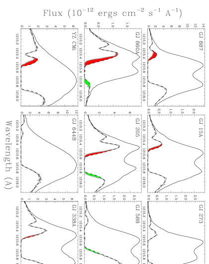
The H I Lyman- $\alpha$ lines of our nine target stars are shown in Figure 2. For each profile, the chromospheric emission line is greatly obscured by absorption. This absorption consists of very broad, fully saturated absorption from H I in between the star and Earth, and much narrower absorption from deuterium (D I), which is $-0.33$ Å blueward of the H I absorption. The D I absorption is entirely interstellar, but the H I absorption can include contributions from heliospheric and/or astrospheric absorption. It should be noted that narrow geocoronal Lyman- $\alpha$ emission has been removed from the spectra. This removal can be problematic if the geocoronal emission is blended with any of the emission observed from the star (Wood et al., 2005b). However, for all our observations the geocoronal emission is a weak, narrow emission line completely within the saturated core of the ISM absorption, unblended with any of the stellar emission and therefore easy to remove.

Hydrogen is the only element abundant enough for the heliospheric and/or astrospheric (HS/AS) absorption signature to be detectable. In the analysis of the Lyman- $\alpha$ lines, the D I absorption is crucial, as the presence of HS/AS absorption reveals itself through discrepancies between the H I and D I absorption profiles. Our analysis mirrors many past studies, and is described most extensively in Wood et al. (2005b). The H I and D I absorption lines are fitted simultaneously using $\chi^{2}$ minimization, taking into account the two hyperfine components of the H I and D I lines. We force the H I and D I absorption features to have self-consistent central velocities [e.g., $v({\rm HI})=v({\rm DI})$ ] and Doppler parameters. Given that the H I and D I lines are dominated by thermal broadening, the latter constraint means that $b({\rm HI})=\sqrt{2}\times b({\rm DI})$ . Finally, the D/H ratio has been found to be constant within the LB, with a value of ${\rm D/H}=1.56\times 10^{-5}$ (Wood et al., 2004), so in the fits we force the column density ratio of D I to H I to be consistent with this value. In this way, all three of the H I parameters are actually related to D I, meaning that in a single-component fit to the H I+D I absorption there are actually only three free parameters.

In the few cases where the Mg II analysis has indicated multiple ISM components (see Table 2), we include these components in the Lyman- $\alpha$ analysis, though the components are hopelessly blended in the broader H I and D I lines. In the H I+D I fits, the velocity separation of the components is forced to be consistent with the Mg II fit. For simplicity, we also simply force the components to have the same column density ratio as in the Mg II fit, and we assume that the components have identical Doppler parameters. Parameters fixed in this fashion are identified with parentheses in Table 2.

The Lyman- $\alpha$ analysis not only involves fitting the absorption, but also reconstructing the intrinsic stellar Lyman- $\alpha$ profile in the process, which is not trivial considering the broad extent of the H I absorption. In the $\log N({\rm HI})\approx 18.0$ column density regime represented by our nearby target stars, the Lorentzian natural line opacity profile is relevant as well as the Gaussian thermal Doppler core. The full opacity profile is a Voigt profile, which is a convolution of the Lorentzian and Gaussian components. The wing absorption apparent far from line center in Figure 2 is associated with the former, while the Doppler core of the opacity profile affects the width of the saturated core of the absorption.

In the analysis, an initial guess is made for the background shape of the stellar Lyman- $\alpha$ line, with guidance from the profile of the Mg II lines, which like Lyman- $\alpha$ are highly opaque chromospheric resonance lines that have similar profiles in the solar spectrum. After an initial fit is made to the data, the residuals of the fit are then used to modify the assumed stellar line profile to improve the fit. Further iterations are made, if necessary. The self-reversals inferred from Mg II are generally preserved in this process, but in practice the absorption fit parameters are little affected by the exact shape of the stellar profile near line center.

Every effort is made to find an acceptable fit to the data assuming only ISM absorption. However, we are successful in only two of the nine cases, GJ 273 and GJ 644B. For the other stars, the ISM-only fits are poor, presumably due to the presence of HS/AS absorption contributing to the H I absorption but not D I. Using YZ CMi as an example, Figure 3(a) explicitly shows the best ISM-only fit to the data, which is clearly unacceptable. The fitted D I absorption is too broad. This implies that the widths of the H I and D I absorption are inconsistent, with H I too broad relative to D I. In other words, there must be excess H I absorption beyond that from the ISM, but not D I because of the much lower column density in this line. Furthermore, the fitted D I absorption profile is blueshifted relative to the observed absorption, suggesting that the excess H I absorption is primarily on the blue side of the line, which is indicative of an astrospheric absorption detection.

The heliospheric and astrospheric absorption produce excess absorption on opposite sides of the ISM absorption, allowing us to the distinguish between the two. When detectable, the heliospheric absorption is apparent as excess absorption on the right side of the ISM absorption. This redshift is due to the deceleration and deflection of ISM material as it approaches the heliopause. In contrast, the astrospheric absorption is blueshifted relative to the ISM absorption for the same reason, with the difference being due to our viewpoint outside the astrosphere instead of inside.

For the seven cases where HS/AS absorption is present, it is necessary to estimate the nature of the excess H I absorption with another fit. For this purpose, we add another absorption component to the fit that is designed to approximate the HS/AS absorption regardless of whether the excess absorption is heliospheric, astrospheric, or some combination of the two. Figure 3(b) shows an example of the resulting fit for YZ CMi, consistent with excess absorption on the blue side of the line, which is the astrospheric signature. There is a hint of excess on the red side of the line as well, which could be a sign of heliospheric absorption, but we do not consider the excess sufficiently convincing to deem this a heliospheric detection.

As shown in Figure 2, we find evidence for astrospheric signatures in six of the spectra (GJ 887, GJ 15A, GJ 860A, GJ 205, YZ CMi, and GJ 338A) and heliospheric signatures in only three cases (GJ 860A, GJ 205, and GJ 588). The detectability of heliospheric absorption depends primarily on two factors. The first is the ISM H I column density, which if high enough will broaden the ISM absorption enough to obscure the heliospheric signature. The second is the angle of the LOS relative to the ISM flow direction seen by the Sun, with the heliospheric absorption much easier to detect closer to upwind directions (Wood et al., 2005b). For the three heliospheric detections, we verify that the inferred heliospheric absorption is consistent with expectations by comparing the observed excess absorption with that predicted by a heliospheric model from Wood et al. (2000), which we have found in past analyses to be successful in reproducing observed heliospheric Lyman- $\alpha$ absorption. We will say little more about the heliospheric absorption, as we are here more interested in the astrospheric detections and what they imply about the winds of their associated stars.

The final H I Lyman- $\alpha$ fit parameters are listed in Table 2. We include the parameters of the HS/AS components, although the properties of the heliosphere and/or astrosphere cannot be successfully quantified using fits of this nature. Hydrodynamic models are required for any meaningful quantitative analysis of the HS/AS absorption, as will be described in the next section.

Finally, we note in passing that the intrinsic stellar Lyman- $\alpha$ profiles are also useful products of this analysis. From such profiles, integrated Lyman- $\alpha$ line fluxes can be measured, which are excellent diagnostics of stellar chromospheric activity. The Lyman- $\alpha$ line fluxes from our analysis are listed and discussed by Melbourne et al. (2020) and Linsky et al. (2020).

4 Analysis of M Dwarf Astrospheric Absorption

4.1 Summary of M Dwarf Wind Constraints from HST

Table 3: Mass Loss Measurements for Coronal Winds

ID #	Star	Spectral	$d$	$V_{ISM}$	$\theta$	$\dot{M}$	log L_x	Radius
		Type	(pc)	(km s^-1)	(deg)	( $\dot{M}_{\odot}$ )		(R_⊙)
M DWARFS
1	Prox Cen	M5.5 V	1.30	25	79	$<0.2$	27.22	0.14
2	GJ 699^a^aNew analysis.	M4 V	1.83	121	43	$<0.2$	25.85	0.19
3	GJ 411^a^aNew analysis.	M2 V	2.55	110	36	$<0.1$	26.89	0.36
4	GJ 729	M3.5 V	2.98	11	178	…	27.06	0.20
5	GJ 887^a^aNew analysis.	M2 V	3.29	85	99	0.5	27.03	0.47
6	GJ 15AB^a^aNew analysis.	M2 V+M3.5 V	3.56	28	95	10	27.37	0.37+0.17
7	GJ 273^a^aNew analysis.	M3.5 V	3.80	75	89	$<0.2$	26.54	0.31
8	GJ 860AB^a^aNew analysis.	M3 V+M4 V	4.01	47	55	0.15	27.72	0.29+0.26
9	AD Leo	M4 V	4.97	13	114	…	28.80	0.39
10	EV Lac	M3.5 V	5.05	45	84	1	28.99	0.32
11	GJ 205^a^aNew analysis.	M1.5 V	5.70	70	79	0.3	27.66	0.59
12	GJ 588^a^aNew analysis.	M2.5 V	5.92	47	139	$<5$	27.00	0.43
13	YZ CMi^a^aNew analysis.	M4 V	5.99	20	114	30	28.57	0.33
14	GJ 644AB^a^aNew analysis.	M3+M4+M4 V	6.20	53	136	$<5$	29.04	0.3+0.3+0.3
15	GJ 338AB^a^aNew analysis.	M0 V+M0 V	6.33	29	88	0.5	27.92	0.60+0.60
16	GJ 436^b^bExoplanet transit absorption.	M3 V	9.75	79	97	0.059	26.76	0.40
17	GJ 173	M1 V	11.2	38	43	0.75	26.84	0.42
GK STARS
18	$\alpha$ Cen AB	G2 V+K0 V	1.35	25	79	0.46+1.54	26.99+27.32	1.22+0.86
19	$\epsilon$ Eri	K2 V	3.22	27	76	30	28.31	0.74
20	61 Cyg A	K5 V	3.48	86	46	0.5	27.03	0.67
21	$\epsilon$ Ind	K5 V	3.63	68	64	0.5	27.39	0.73
22	$\tau$ Cet	G8 V	3.65	56	59	$<0.1$	26.69	0.77
23	70 Oph AB	K0 V+K5 V	5.09	37	120	55.7+44.3	28.09+27.97	0.83+0.67
24	36 Oph AB	K1 V+K1 V	5.99	40	134	8.5+6.5	28.02+27.89	0.69+0.59
25	$\delta$ Pav	G8 IV	6.11	29	72	10	27.29	1.22
26	GJ 892	K3 V	6.55	49	60	0.5	26.85	0.78
27	$\xi$ Boo AB	G8 V+K4 V	6.70	32	131	0.5+4.5	28.91+28.08	0.86+0.61
28	61 Vir	G5 V	8.53	51	98	0.3	26.87	0.99
29	$\delta$ Eri	K0 IV	9.04	37	41	4	27.05	2.58
30	$\pi^{1}$ UMa	G1.5 V	14.4	43	34	0.5	28.99	0.97
31	$\lambda$ And	G8 IV-III	25.8	53	89	5	30.82	7.40
32	DK UMa	G4 III-IV	32.4	43	32	0.15	30.36	4.40
SLINGSHOT PROMINENCE STARS
33	V374 Peg	M3.5 V	9.1	9	85	200	28.45	0.34
34	AB Dor	K0 V	15.3	31	157	350	29.87	0.93
35	HK Aqr	M0 V	24.9	14	110	50	29.01	0.59
36	Speedy Mic	K3 V	66.7	25	109	130	31.06	1.06
37	LQ Lup	G8 IV	146.7	24	165	4500	30.90	1.30

The central goal of our project is to characterize the winds of M dwarf stars using all available constraints. To that end, in the top section of Table 3 we have compiled a list of all M dwarfs with relevant Lyman- $\alpha$ observations from HST that can at least in principle yield wind constraints. We include stars within 7 pc that are nondetections, since within 7 pc nondetections can possibly provide upper limits for $\dot{M}$ (see Section 2). Stars listed include the ones mentioned in Section 1, namely the astrospheric absorption detections for EV Lac and GJ 173 (Wood et al., 2005a, Vannier et al., in preparation), and the transiting exoplanet absorption constraint for GJ 436 (Vidotto & Bourrier, 2017). Also listed is the upper limit for Proxima Cen from Wood et al. (2001). Another astrospheric nondetection, AD Leo, is also listed (Wood et al., 2005b), and we here assess whether these data can provide a useful $\dot{M}$ upper limit.

The nine target stars of our new HST observing program account for most of the rest of the M dwarfs in Table 3. The exceptions are three additional very nearby stars. These include GJ 729, which is part of the Mega-MUSCLES project (HST program GO-15071: Melbourne et al., 2020; Linsky et al., 2020). The other two are GJ 699 and GJ 411, the analysis of which will be described elsewhere (Youngblood et al., in preparation). They and GJ 729 are all astrospheric nondetections, and like the AD Leo case noted above we here try to infer upper limits for $\dot{M}$ . The second section of Table 3 lists other $\dot{M}$ measurements from astrospheric Lyman- $\alpha$ constraints, as previously compiled by Wood (2018). Finally, the bottom section lists slingshot prominence stars with $\dot{M}$ measurements, from Jardine & Collier Cameron (2019).

In the case of binary stars, the companion stars are listed if they are nearby enough that both stars will lie within the same astrosphere, meaning that the astrospheric absorption will be a diagnostic of the combined winds of both stars. For example, the GJ 860AB binary (M3 V+M4 V) has a separation of only $2.4^{\prime\prime}$ , corresponding to a plane-of-sky distance of only 9.6 au, easily close enough for both stars to reside within the same astrosphere. For GJ 644AB, there are actually three stars involved, with the observed spectroscopic binary GJ 644B (M4 V+M4 V) separated from GJ 644A (M3 V) by $0.23^{\prime\prime}$ , corresponding to a distance of only 1.5 au.

The $V_{ISM}$ quantity in Table 3 is the ISM flow speed seen by the star in stellar rest frame, and $\theta$ is the angle betwen the upwind direction of the ISM flow and our LOS to the star. These are quantities that must be known to infer $\dot{M}$ from an astrospheric absorption detection, as will become clear in Section 4.2. Computing $V_{ISM}$ and $\theta$ requires knowledge of the stellar radial velocity and proper motion (very well known for such nearby stars, and obtainable from the SIMBAD database), and the LIC flow vector from Redfield & Linsky (2008). Given that multiple ISM velocity components are often seen toward even very nearby stars, other ISM flow vectors besides that of the LIC clearly exist near the Sun, and may exist around some of our observed stars, particularly the ones with multiple Mg II components (see Figure 1). However, within 7 pc the multiple ISM components, when present, are generally closely spaced in velocity, meaning that the different ISM vectors are similar. Thus, our universal assumption of the LIC vector should be a decent approximation. As an example, the existence of Aur cloud absorption toward GJ 273 means that GJ 273 probably lies within the Aur cloud instead of the LIC. Using the Aur cloud vector from Redfield & Linsky (2008), we estimate $V_{ISM}=65$ km s^-1 and $\theta=86^{\circ}$ for GJ 273, representing only a small change from the $V_{ISM}=75$ km s^-1 and $\theta=89^{\circ}$ values computed using the LIC vector.

The $\dot{M}$ column in Table 3 lists inferred mass loss rates, with new results being described below in Section 4.2. For four of the previously studied binaries, the $\dot{M}$ has been divided between the two stars, as described by Wood (2018). We will be seeking to relate $\dot{M}$ to coronal activity, so coronal X-ray luminosities (in ergs s^-1) are also listed, based mostly on ROSAT all-sky survey measurements (Schmitt & Liefke, 2004). For binaries that have been resolved in X-rays, we list separate $\log L_{X}$ values for both stars.

Finally, when comparing $\dot{M}$ and $\log L_{X}$ for stars of different sizes, it is appropriate to normalize by stellar surface area, so we also list in Table 3 the stellar radii that we are assuming. For the M dwarfs, the radii are mostly from Houdebine et al. (2019). However, for GJ 644AB no individual radii measurements exist for the three individual stars in this system, so we simply assume a typical radius for mid-M dwarfs, $R=0.3$ R_⊙, for all three stars.

4.2 Hydrodynamic Modeling of Astrospheres

Our HST survey of nearby M dwarfs has yielded detections of astrospheric absorption in six of nine cases. The 67% astrospheric detection percentage is consistent with the high detection fraction previously found for stars within 7 pc (Wood, 2018). This in turn is consistent with the notion that the local ISM within 7 pc is predominantly like the warm, partly neutral ISM known to surround the Sun, as opposed to the fully ionized ISM that more generally characterizes the LB. It is therefore likely that the three nondetections of astrospheric absorption are due to weak stellar winds, meaning that we will be able to infer upper limits for the stellar wind mass-loss rates for these nondetections.

Estimating stellar mass-loss rates from astrospheric absorption requires guidance from hydrodynamic models of the astrosphere, analogous to models of the global heliosphere that have been computed for decades to confront heliospheric observations from spacecraft such as Voyager and the Interstellar Boundary Explorer (IBEX). Analogous to past studies (Wood et al., 2005a, 2014), the code we use to model the astrospheres is a 2.5-D axisymmetric, multi-fluid code that treats the plasma as a single fluid, but the neutral hydrogen as multiple fluids corresponding to distinct heliospheric regions in which charge exchange yields different populations of neutrals, which do not equilibrate with the plasma or with each other due to the low densities (Zank et al., 1996). The neutral and plasma fluids interact primarily through charge exchange interactions, involving an electron jumping from a neutral H atom to a proton.

The heliospheric model that has long represented the starting point for our analysis is one that has consistently demonstrated its ability to reproduce heliospheric absorption detected for various lines of sight in various directions while assuming plausible values for the ISM boundary conditions of the heliosphere, including the local ISM’s flow velocity in the solar rest frame, $V_{ISM}=26$ km s^-1 (Wood et al., 2000, 2005b). We have already noted its success in reproducing the heliospheric absorption seen for three of our nine observed lines of sight.

An astrospheric model assuming a solar mass-loss rate is computed by changing $V_{ISM}$ in the heliospheric model to the value appropriate for the star (see Table 3), while keeping everything else the same. In order to experiment with different assumed stellar mass-loss rates, we simply vary the assumed stellar wind density at the inner boundary, which is typically at 1 au from the star. From such models we can compute the absorption predicted by the model by integrating along the LOS through the astrosphere, with a direction defined by the $\theta$ value in Table 3. Higher $\dot{M}$ values naturally lead to larger astrospheres, larger hydrogen wall column densities, and therefore more Lyman- $\alpha$ absorption. Rather than varying the stellar wind density to modify $\dot{M}$ , we could alternatively vary the stellar wind velocity, $V_{w}$ . However, along the lower main sequence stellar mass and radius happen to vary in such a way that the surface escape speed is relatively constant. This provides some reason to believe that the winds of lower main sequence stars might all have similar speeds, given that the solar wind velocity is similar to the Sun’s surface escape speed of 618 km s^-1. The astrospheric absorption is to first order determined by the size scale of the astrosphere, which depends on the stellar wind ram pressure, $P_{w}$ . Since $P_{w}\propto\dot{M}V_{w}$ , mass loss rate estimates will vary inversely with the assumed $V_{w}$ (Wood et al., 2002).

We have in the past estimated that $\dot{M}$ values measured in this way should be accurate to within about a factor of two (Wood et al., 2005a), with important systematic uncertainties including the unknown degree of variation in ISM properties from star to star, and possible differences in stellar wind speed. The accuracy of the physics in the heliospheric/astrospheric modeling code is another source of uncertainty, but this model dependence is not as crucial as one might suppose, because the approach of extrapolating the astrospheric models from a heliospheric model that reproduces the heliospheric absorption makes the procedure somewhat semi-empirical. The physics of how an astrosphere’s size and Lyman- $\alpha$ absorption properties respond to changes in $V_{ISM}$ and stellar wind density is relatively simple, depending on the balance of ram pressure between the two flows, so these changes should be relatively insensitive to the details of the physics in the model being used. Thus, there is little reason to believe that replacing our code with more sophisticated ones that are now available would change our conclusions significantly. More sophisticated models include ones that are fully 3-D, including heliospheric and ISM magnetic fields, and ones with a fully kinetic treatment of the neutrals (e.g., Izmodenov et al., 2009; Pogorelov et al., 2013; Opher et al., 2015).

Figure 4 shows the Lyman- $\alpha$ lines of the six M dwarfs with newly detected astrospheric absorption, zooming in on the blue side of the H I absorption profile where the astrospheric absorption lies. The figure also shows the absorption predicted by a variety of astrospheric models with different assumed mass-loss rates, after being added to the ISM absorption. Astrospheric absorption naturally increases as $\dot{M}$ is increased, due to a larger astrosphere with a thicker hydrogen wall and higher H I column densities along the observed LOS through the astrosphere.

Judging which model best reproduces the observed absorption involves some degree of subjectivity. The discrepancy with the data naturally varies along the side of the H I absorption profile. It is generally more important to fit the data near the base of the absorption than higher along the side of the profile, because reasonable adjustments to the shape of the assumed stellar Lyman- $\alpha$ emission profile can in principle improve discrepancies at higher flux levels. Such corrections are harder near the base of the absorption, as the necessary adjustments to the stellar profile would introduce implausible fine structure into the profile.

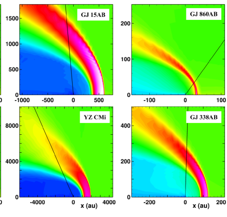
The $\dot{M}$ values that best fit the data are listed in Table 3, and Figure 5 shows H I density maps for the best-fit astrospheric models. The highest H I densities along the LOS to the star are in the hydrogen wall region, which is the parabola-shaped reddish (or purplish-red) region seen in each panel. This is where the ISM material is piled up outside of the stellar astropause, with the outer edge of the hydrogen wall marking the location of the stellar bow shock. It is this hydrogen wall region that generally dominates the astrospheric absorption signature, not just due to the higher H I densities, but also due to the decelerated flow speeds and relatively high temperatures at that location. As the ISM passes through the stellar bow shock, it is heated as well as compressed and decelerated. (It turns out that the situation is somewhat different for YZ CMi, as will be described in Section 4.3.)

The size of the astrospheres in Figure 5 varies tremendously, depending on both $V_{ISM}$ and $\dot{M}$ . The smallest astrosphere is that of GJ 205, with an upwind bow shock distance of only about 30 au, due to both a high ISM flow speed of $V_{ISM}=70$ km s^-1 and a low mass-loss rate of $\dot{M}=0.3$ $\dot{M}_{\odot}$ . This can be compared with the huge astrosphere of YZ CMi, with an upwind bow shock distance of 2000 au, due to both a low ISM flow speed of $V_{ISM}=20$ km s^-1 and a high mass-loss rate of $\dot{M}=30$ $\dot{M}_{\odot}$ . It is from these best-fit astrosphere models that we can confirm that the astrospheres of the binaries GJ 15AB, GJ 860AB, and GJ 338AB are indeed large enough to encompass both members of the binary, meaning that the stellar wind that is being diagnosed is that of the combined winds of both stars.

Turning our attention to the astrospheric nondetections within 7 pc, we note that there are eight of these listed in Table 3. For one of them, Proxima Cen, there is already a published upper limit of $\dot{M}<0.2$ $\dot{M}_{\odot}$ . We now seek to infer upper limits for the other seven stars. For GJ 729 and AD Leo, we ultimately conclude that no useful $\dot{M}$ constraints can be inferred, primarily due to the very low $V_{ISM}$ values for these stars (see Table 3). This greatly complicates the astrospheric modeling, in part due to the kinds of physical effects discussed in the next subsection about YZ CMi, which also has low $V_{ISM}$ (though not nearly as low as GJ 729 and AD Leo).

The Lyman- $\alpha$ spectra of the remaining five M dwarf astrospheric nondetections are shown in Figure 6, where we are once again zooming in on the blue side of the H I absorption line where the astrospheric absorption would be if any had been detected. We note again that the original analyses of GJ 699 and GJ 411 are presented elsewhere (Youngblood et al., in preparation). For each star, models are constructed assuming different $\dot{M}$ to see how large $\dot{M}$ must be for there to have been detectable astrospheric absorption for the observed LOS. Analogous to the situation for the astrospheric detections, there is some subjectivity in deciding how much excess astrospheric absorption must be predicted beyond that from the ISM before it should be considered detectable. Figure 6 illustrates the predicted absorption of the models that we decide represent the upper limits. These range from $\dot{M}<0.1$ $\dot{M}_{\odot}$ for GJ 411 to $\dot{M}<5$ $\dot{M}_{\odot}$ for GJ 588 and GJ 644AB.

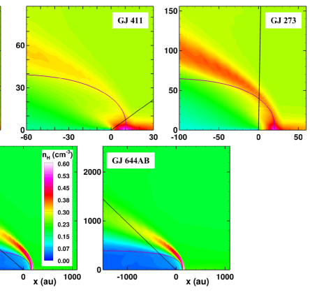
The H I number density maps of the upper limit astrospheric models are shown in Figure 7. The lines of sight to GJ 588 and GJ 644AB are particularly downwind, which is not advantageous for detecting astrospheric absorption, missing the most detectable part of the hydrogen wall. This in part explains the relatively high upper limits for $\dot{M}$ for these stars. The upper limit models for GJ 699 and GJ 411 have upwind bow shock distances of only about 10 au, due primarily to high $V_{ISM}$ . Considering that these are upper limits, these astrospheres are clearly very small, easily the most compact astrospheres inferred so far using the astrospheric Lyman- $\alpha$ absorption diagnostic.

Considering all the M dwarf $\dot{M}$ constraints from Table 3 together, we now have actual $\dot{M}$ measurements for nine stars, and upper limits for six. For 13 of the 15 M dwarfs, the results are consistent with the winds being comparable or weaker to the solar wind. Weak winds for M dwarfs are not surprising, considering the small size of these stars. However, M dwarfs can be surprisingly active, with frequent and energetic flares, so higher $\dot{M}$ values might have been expected as well. There are two M dwarf $\dot{M}$ measurements that clearly stick out for being unusually high: GJ 15AB with $\dot{M}=10$ $\dot{M}_{\odot}$ , and YZ CMi with $\dot{M}=30$ $\dot{M}_{\odot}$ . Before discussing the implications of these results further, it is necessary to discuss some important and unique characteristics of the YZ CMi astrosphere.

4.3 YZ CMi: New Physics for Astrospheric Absorption

Heliospheric and astrospheric Lyman- $\alpha$ absorption has been detected for many lines of sight toward nearby stars, despite H I column densities that are $3-5$ orders of magnitude lower than the ISM H I column densities for these lines of sight. Astrospheric absorption is nevertheless detectable because as the ISM approaches an astrosphere, it is heated and decelerated as it nears the astropause, which is the boundary separating the plasma flows of the stellar wind and the ISM. The heating results in a broader absorption profile, which helps to extend the astrospheric absorption in wavelength beyond that from the ISM, and the deceleration shifts the absorption blueward, creating the excess blue-side absorption that characterizes the astrospheric absorption signature.

Both the heating and deceleration effects are highly dependent on the ISM flow speed seen by the star, $V_{ISM}$ . The Sun sees $V_{ISM}=26.08\pm 0.21$ km s^-1 (Wood et al., 2015). This happens to correspond to a flow with a Mach number of $M\approx 1$ , leading to much debate in the space physics community about whether there is a bow shock in front of the heliosphere, or whether no real shock exists and that the pile-up region outside the heliopause is better characterized as a “bow wave” (Zank et al., 2013). Even without a bow shock, there will still be adiabatic deceleration, compression, and heating of the material in the bow wave, and there is no truly dramatic decrease in heliospheric absorption for the bow wave case with $M\approx 1$ compared to a bow shock case with $M\approx 1$ (Zank et al., 2013). Nevertheless, it is no accident that nearly all the astrospheric detections listed in Table 3 have $V_{ISM}$ higher than the solar example. This makes the existence of a bow shock far less ambiguous than for the Sun, producing more heating and deceleration of the ISM outside the astropause than the solar case, making the astrospheric absorption more detectable.

In selecting targets for our HST M dwarf observing program, we tried to avoid stars with low $V_{ISM}$ . Nevertheless, an exception was made for YZ CMi. For our sample, we wanted to include at least a couple very active M dwarfs, which still had to be within 7 pc for reasons discussed in Section 2. The best available target after GJ 644 was YZ CMi. We have been rewarded for this choice by the clear detection of astrospheric absorption for this star (see Figure 3), despite the low $V_{ISM}=20$ km s^-1 value. Furthermore, our astrospheric models are indeed able to reproduce the absorption well, with a sufficiently high mass-loss rate of $\dot{M}=30$ $\dot{M}_{\odot}$ (see Figure 4). However, examination of the YZ CMi astrospheric model reveals that the astrospheric absorption has an origin somewhat different from other astrospheric detections, which requires more discussion.

Like all other cases of astrospheric absorption, hydrogen wall neutrals are the source of the absorption, which are a population of neutral H created by charge exchange with the ISM protons that have been heated by passage through the bow shock (or by compression in the bow wave). The difference for YZ CMi is that the absorption is not coming primarily from the hydrogen wall itself, where neutral H densities are highest (the yellow and reddish region along the LOS in Figure 5), but from neutrals very near and inside the astropause (the blue and green region along the LOS in Figure 5). The neutrals have an unexpectedly high temperature in this location, explaining why they produce more absorption than the bulk of the particle population in the hydrogen wall region.

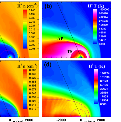
To explore this further, Figure 8 shows maps of number density and temperature for protons (H⁺) and for neutral H (H⁰), for the $\dot{M}=30$ $\dot{M}_{\odot}$ YZ CMi model. The H⁺ and H⁰ temperatures within the hydrogen wall are generally rather low, $T\approx 15,000$ K. Such temperatures are expected, given the low $V_{ISM}=20$ km s^-1 speed of the ISM flow, and are not conducive to producing detectable astrospheric absorption. Another problem is the less-than-ideal crosswind LOS to the star. There will be some blueward shift of the hydrogen wall flow relative to the ISM flow, due to deflection around the astrosphere, but not as much as if the LOS were upwind. In short, it is questionable whether the YZ CMi hydrogen wall could yield detectable astrospheric absorption even for high values of $\dot{M}$ .

However, the $H^{+}$ temperature is actually surprisingly high just outside the astropause, with $T\approx 6\times 10^{4}$ K. Although densities are significantly lower here, the large size of the astrosphere means that there is still a significant amount of charge exchange happening, thereby creating significant numbers of hydrogen wall neutrals with these high temperatures, some of which can cross the astropause and dominate the part of the LOS inside the astropause. Since our multi-fluid code uses a single Maxwellian fluid to represent all neutrals produced by charge exchange within the hydrogen wall, the mixture of hot neutrals produced very close to the astropause with the cooler neutrals produced in the bulk of the hydrogen wall yield H⁰ temperatures along the LOS that are $T=30,000-50,000$ K near and inside the astropause (see Figure 8d). Despite the relatively low H⁰ densities in this area, the huge astrospheric size means that there is still sufficient H I column density for these neutrals to yield detectable absorption. This absorption exceeds that from the much denser, but much cooler, hydrogen wall itself, and this is actually the source of the absorption shown in Figure 4.

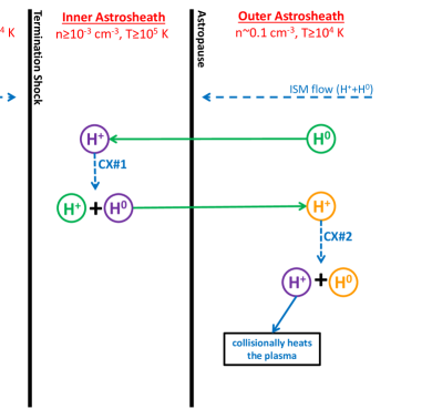
The conclusion is that the immediate source of the astrospheric absorption signature for YZ CMi is charge exchange with this surprisingly hot H⁺ just outside the astropause. But what is heating the H⁺ there? The answer is that it is being heated by outward heat transport across the astropause from neutrals created by charge exchange inside the astropause, some of which then cross the astropause and dump their energy outside of it via another charge exchange interaction. Figure 9 provides an illustration of the sequence of two charge exchange interactions that allow this to happen. The inner astrosheath region just inside the astropause is very hot, as it is characterized by stellar wind that is heated significantly by its passage through the termination shock. However, this region has very low densities (see Figure 8a). Although ISM neutrals can penetrate the astropause and charge exchange there, in most cases there are too few of these interactions for them to be important. However, the YZ CMi astrosphere in Figure 8 is so large that there are enough of these inner astrosheath neutrals created to transport significant amounts of energy out of the inner astrosheath and into the part of the hydrogen wall just outside the astropause, with the energy deposited via another charge exchange reaction. Potential effects of this kind of anomalous heating have been discussed before in the context of heliospheric models (e.g., Zank et al., 2013), but with YZ CMi we have for the first time encountered a case where this heating across the astropause has become more important than any heating occurring within the actual bow shock/wave, with regards to yielding detectable H I absorption.

One downside to the different physics involved in the YZ CMi astrospheric absorption signature is that it undoubtedly increases the uncertainty in our $\dot{M}$ measurement. The arguments in Section 4.2 about the relative unimportance of model dependence for the $\dot{M}$ measurements no longer apply, since the physics of the YZ CMi absorption is significantly different from the physics of the heliospheric Lyman- $\alpha$ absorption in the baseline heliospheric model, from which all of the astrospheric models are basically extrapolated. This is definitely a case where further modeling efforts would be worthwhile, particularly models that include a fully kinetic treatment of the neutrals. The enhanced uncertainty in the YZ CMi measurement is problematic considering how important this measurement potentially is, representing the highest $\dot{M}$ per unit surface area yet detected via the astrospheric Lyman- $\alpha$ absorption diagnostic. Nevertheless, in our discussion of the ramifications of our new $\dot{M}$ measurements in the next section, the high YZ CMi $\dot{M}$ measurement will be assumed valid.

5 Implications of the M Dwarf Wind Measurements

5.1 Relating $\dot{M}$ and Coronal Activity

With the new M dwarf $\dot{M}$ measurements provided here, we can try to characterize the winds of M dwarfs for the first time. This is most naturally done in a plot like Figure 10, showing mass loss rate per unit surface area plotted versus X-ray surface flux. This is done not only for the M dwarfs, but for the other stars listed in Table 3 as well. For the solar data point, the mean solar X-ray luminosity assumed is from Judge et al. (2003). This would vary by about a factor of 4 over the course of the activity cycle (Ayres, 2020).

Trying to relate $\dot{M}$ with $F_{X}$ is natural, given that hot coronae represent the source regions of coronal winds. The existence and basic characteristics of the solar wind can to first order be understood as simple thermal expansion from the hot solar corona (Parker, 1958). Nevertheless, it is far from obvious a priori that $\dot{M}$ and $F_{X}$ should be correlated, given that coronal X-ray emission originates from coronal loops, which are closed magnetic fields with both footpoints tied to the photosphere, while coronal wind will be coming from open field regions with only one footpoint tied to the photosphere and the other end of the field line extending out into the astrosphere. For the Sun, no correlation between $\dot{M}$ and $F_{X}$ is observed during the solar activity cycle (Cohen, 2011).

Nevertheless, Figure 10 seems to show a general trend of increasing $\dot{M}$ with $F_{X}$ , albeit with lots of scatter. A power law fit to the data points, excluding the subgiant/giant stars, yields $\dot{M}\propto F_{X}^{0.77\pm 0.04}$ , as shown in the figure. This is a somewhat flatter relation than the $\dot{M}\propto F_{X}^{1.34\pm 0.18}$ result previously reported for the GK stars alone, excluding $\xi$ Boo A and $\pi^{1}$ UMa (Wood et al., 2005a). The impression of a wide range of $\dot{M}$ at a given $F_{X}$ value is greatly increased with the inclusion of the numerous new M dwarf data points. The M dwarf measurements suggest that main sequence stars with a given $F_{X}$ value can have $\dot{M}$ values that vary by up to two orders of magnitude. This impression relies heavily on the two M dwarfs with surprisingly strong winds, GJ 15AB (star #6) with $\dot{M}=10$ $\dot{M}_{\odot}$ and YZ CMi (star #13) with $\dot{M}=30$ $\dot{M}_{\odot}$ . The GJ 15AB measurement is well over an order of magnitude higher than the $\dot{M}=0.15-0.5$ $\dot{M}_{\odot}$ measurements for GJ 860AB, GJ 205, and GJ 338AB (stars #8, #11, and #15), which have similar $F_{X}$ . At a higher activity level, the YZ CMi measurement is 30 times higher than that of EV Lac (star #10), despite similar $F_{X}$ .

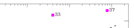
The YZ CMi data point is also notable for being the one astrospheric Lyman- $\alpha$ measurement that overlaps with the region of Figure 10 occupied by the slingshot prominence winds. The slingshot prominence stars are all characterized by extremely rapid rotation. The fastest rotator among the stars with astrospheric measurements is indeed YZ CMi, with $P_{rot}=2.78$ days (Diez Alonso et al., 2019), but this is still much slower than the slingshot prominence stars, with $P_{rot}\leq 0.5$ days (Jardine & Collier Cameron, 2019). Nevertheless, Villarreal D’Angelo et al. (2018) find that both YZ CMi and EV Lac are rotating fast enough to be in the centrifugal confinement regime that could allow the slingshot prominence phenomenon to exist, and they estimate potential mass loss rates for YZ CMi and EV Lac of up to $\dot{M}=0.7$ $\dot{M}_{\odot}$ and $\dot{M}=0.28$ $\dot{M}_{\odot}$ , respectively. These are lower than our measurements, and therefore consistent. It is possible that some fraction of the wind that we are detecting for YZ CMi and EV Lac could consist of slingshot prominence material.

Considering only the GK dwarfs in Figure 10, the impression is of a comparatively tight relation between $\dot{M}$ and $F_{X}$ for $\log F_{X}<6.0$ , with the two surprisingly low $\dot{M}$ values with $\log F_{X}>6.0$ suggesting a change of behavior in the $\dot{M}$ - $F_{X}$ relation for $\log F_{X}>6.0$ . In the past, this had been referred to as a possible “wind dividing line” (Wood et al., 2005a, 2014). The existence of such a dividing line is clearly weakened by the new M dwarf measurements. With their inclusion, the two low GK dwarf data points no longer appear clearly inconsistent with the high GK dwarf measurements seen at slightly lower activity, given the high degree of scatter apparent in the loose $\dot{M}$ - $F_{X}$ relation.

The $\dot{M}$ measurements available to date now imply that coronal wind strength is not dependent solely on spectral type and coronal activity, though this inference relies heavily on just two of the new M dwarf measurements. Without the GJ 15AB and YZ CMi data points, Figure 10 would suggest that M dwarfs all have rather low $\dot{M}$ , regardless of activity, and their winds may be exhibiting different behavior compared to the GK dwarf winds at moderate to high activity. With only two strong M dwarf winds found to date, it would be helpful in the future if other examples of strong M dwarf winds could be found, to provide support for the GJ 15AB and YZ CMi measurements.

Our wind measurements can be compared with predictions from theory. For example, Cranmer & Saar (2011) use an Alfvén wave driven wind model to predict mass-loss rates for a wide range of cool stars. However, their predictions for M dwarfs are very low ( $\dot{M}<0.005$ $\dot{M}_{\odot}$ ), clearly inconsistent with our results. Cranmer & Saar (2011) suggest that M dwarf winds may actually be dominated not by Alfvén wave driving, but by CMEs, a possibility we will return to in Section 5.4. Other Alfvén wave based models infer more substantial M dwarf winds, without resorting to CMEs (Vidotto et al., 2014; Alvarado-Gómez et al., 2016; Mesquita & Vidotto, 2020). These models predict increases in wind strength with stellar activity qualitatively consistent with the observed relation in Figure 10, although quantitative comparison with the models is complicated by the extensive scatter in the data. For example, Suzuki et al. (2013) predict $\dot{M}\propto F_{X}^{0.82}$ , in good agreement with the observed $\dot{M}\propto F_{X}^{0.77\pm 0.04}$ . It is possible that mass loss might depend on magnetic complexity as well as disk-averaged magnetic flux (Garraffo et al., 2015), which could in principle contribute to the scatter.

5.2 The Effects of Wind Variability

One possible interpretation of the scatter in the relation between coronal activity and wind strength seen in Figure 10 is that this is due to wind variability. In this interpretation, the discrepancy between the winds of the similar stars EV Lac and YZ CMi is simply due to temporal variability, rather than being indicative of any fundamental difference in wind behavior for these stars. Evalulating this possibility requires an evaluation of the timescale over which our wind measurements are applicable.

This timescale will depend on the length of time it takes a wind ram pressure signal to reach the hydrogen wall region well beyond the astropause. This naturally depends on the size of the astrosphere. For the solar example, it takes the solar wind roughly 6 months to make it to the termination shock, at which point it is decelerated to even slower speeds. This means that it takes many years for any change in solar wind pressure to register at the heliopause. Time-dependent modeling of the heliosphere (e.g., Pogorelov et al., 2013) suggests only a very weak variation in heliopause distance even on activity cycle timescales, and heliospheric absorption is coming from even further distances from the Sun. As a consequence, we do not expect there to be any observable change in heliospheric Lyman- $\alpha$ absorption even on decadal timescales, let alone shorter ones.

Returning to the EV Lac/YZ CMi comparison, the EV Lac astrosphere is somewhat more compact than the heliosphere (Wood et al., 2005a), due to higher $V_{ISM}$ , but the YZ CMi astrosphere is much bigger (see Figure 8). Our large $\dot{M}$ value for YZ CMi will be characteristic of the average mass loss over a period of many decades, if not centuries, depending on the exact stellar wind speed. If the astrosphere of YZ CMi has ever been smaller and characteristic of a weaker wind like that of EV Lac, it has not been for a long time. In general, attributing the scatter in Figure 10 to wind variability seems unlikely due to the lack of sensitivity of the astrospheric wind measurements to short timescale variability.

5.3 Relating $\dot{M}$ and Magnetic Topology

If spectral type and coronal activity level are not solely determinative of $\dot{M}$ , what is the missing factor? One likely candidate is coronal topology. It is possible to envision two stars with similar $F_{X}$ values, but with the coronal emission and associated magnetic field distributed very differently across the stellar surface, which could lead to different wind properties. Exploring this possibility requires knowledge of the magnetic field topology of our sample of stars. Fortunately, information about this is in fact available for many of the stars in the Table 3 sample, thanks to spectropolarimetric measurements (Morin et al., 2008b). A recent survey of such observations for M dwarfs is provided by Kochukhov (2021). In this section, we try to relate our wind measurements to field properties inferred by the spectropolarimetric analyses.

The M dwarfs in our sample with spectropolarimetric constraints are EV Lac (Morin et al., 2008b), YZ CMi (Morin et al., 2008b), Proxima Cen (Klein et al., 2021), and GJ 205 (Hébrard et al., 2016). There are nine other stars in Table 3 with spectropolarimetric measurements. These include studies of 61 Cyg A, $\epsilon$ Eri, $\epsilon$ Ind, $\pi^{1}$ UMa, and $\xi$ Boo AB, which Vidotto et al. (2016) previously sought to relate to wind properties. And finally, we also consider studies of GJ 892 (Folsom et al., 2018), $\lambda$ And (Fionnagáin et al., 2021), and V347 Peg (Morin et al., 2008a), this last star being one of the slingshot prominence stars.

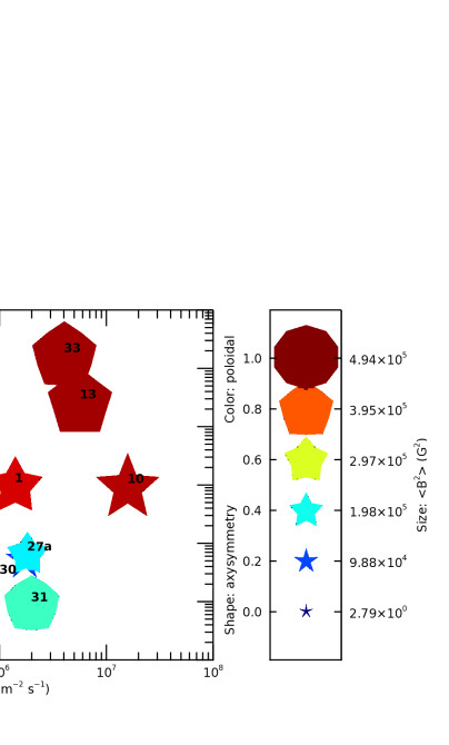
Figure 11 provides an illustration of the spectropolarimetric differences amongst the stars in our sample. It is essentially a reproduction of Figure 10, but with symbols used to indicate various topological properties of the stellar magnetic field inferred from the spectropolarimetry. This is an updated version of a figure from Vidotto et al. (2016). As described by Donati & Landstreet (2009), the size of the symbols indicates the logarithm of the average squared magnetic field ( $\langle B^{2}\rangle$ ), the color of the symbols indicates the relative importance of poloidal and toroidal fields, and the shape of the symbols indicates the degree of axisymmetry of the field. A point is plotted for the Sun at solar minimum (Vidotto, 2016).

As expected, the more active stars with the higher $F_{X}$ values tend to have the stronger fields, as indicated by the larger symbol sizes in Figure 11. There is nevertheless a very wide range in $\dot{M}$ among these more active stars. The three stars with the weakest winds (stars #27a, #30, and #31) have the most toroidal dominant fields, suggesting a possible connection between toroidal fields and weak winds. As for the M dwarf stars that are our focal point here, the EV Lac/YZ CMi comparison is once again of particular interest (stars #10 and #13). The biggest spectropolarimetric difference between these two stars lies in the inferred degree of field axisymmetry, with YZ CMi possessing a very axisymmetric field, and EV Lac exhibiting a strong departure from axisymmetry. It is EV Lac that seems more unusual in the Morin et al. (2008b) sample of M dwarfs, implying that YZ CMi may be more typical of very active M dwarfs. However, EV Lac also is a somewhat slower rotator than the other stars in the sample, with $P_{rot}=4.37$ days. See et al. (2019) estimate similar magnetic filling factors for EV Lac and YZ CMi, although their analysis does not distinguish between open and closed magnetic fields.

The picture of the YZ CMi field provided by Morin et al. (2008b) is that of a highly dipolar, axisymmetric field. However, the spectropolarimetric data is open to interpretation, and Shulyak et al. (2014) provide a somewhat different picture of the overall field topology of YZ CMi. In their analysis, they find evidence for a significant zero-field component for the surface of YZ CMi, in contrast to the other active M dwarfs in their study. This could be interpreted as a stellar analog for coronal holes, which on the Sun are locations of weak surface fields and open field lines where high speed wind streams are escaping.

The EV Lac/YZ CMi dichotomy is not the only example of two seemingly similar active M dwarfs with surprisingly different field properties. Another example is the GJ 65AB binary (BL Ceti+UV Ceti), consisting of two very similar, very active mid-M dwarfs, which nevertheless have very different magnetic topologies (Kochukhov & Lavail, 2018). This difference is likely connected to differences in X-ray and radio behavior for these two coeval stars, which has persisted for decades (Gary & Linsky, 1981; Audard et al., 2003). Ideally, wind measurements would be made for GJ 65A and GJ 65B separately to see how the differences in these coeval stars impact their winds, but the astrospheric absorption technique will not work, as the two stars are close enough to share the same astrosphere, meaning that only the combined strength of the two stellar winds could be measured.

Besides EV Lac and YZ CMi, the only other two M dwarfs in our sample with both astrospheric $\dot{M}$ constraints and spectropolarimetric measurements are GJ 205 (star #11) and Proxima Cen (star #1), which are less active and have much longer rotation periods. The former has a very poloidal, axisymmetric field topology, analogous to YZ CMi, albeit with a much weaker overall field strength, as expected for a more inactive star with a lengthy rotation period of $P_{rot}=33.6$ days. Despite the topological similarities with YZ CMi, the stellar wind of GJ 205 ( $\dot{M}=0.3$ $\dot{M}_{\odot}$ ) is over two orders of magnitude weaker than that of YZ CMi per unit surface area. Like GJ 205, Proxima Cen also has a long rotation period ( $P_{rot}=89.8\pm 4.0$ day) and a wind much weaker than that of YZ CMi ( $\dot{M}<0.2$ $\dot{M}_{\odot}$ ), but unlike GJ 205 its magnetic topology more resembles EV Lac, with significant deviation from axisymmetry.

The large scale field topology of a star is ultimately tied to the properties of its internal dynamo, which also determines the nature of any long-term activity cycle it might have. In studies relating activity cycle periods with rotation rates, there is a suggestion of a bimodality in dynamo operation for stars with relatively fast rotation periods of $P_{rot}<22$ days. The two modes consist of an inactive branch with very short activity cycles ( $P_{cyc}\leq 5$ yr) and an active branch with much longer cycles (Brandenburg et al., 1998; Metcalfe et al., 2016). There is a hint of possible bimodality in Figure 10 as well for the more active stars, separating ones with low $\dot{M}$ and those with high $\dot{M}$ . This impression is particuarly acute for the M dwarfs, with GJ 15AB and YZ CMi having winds over an order of magnitude stronger than all the other M stars. It is worth noting that EV Lac has a reported short activity cycle of $P_{cyc}\approx 5$ yr (Mavridis & Avgoloupis, 1986), while the similarly active YZ CMi, with a much stronger wind, has a much longer activity cycle of $P_{cyc}=27.5$ yr (Bondar & Katsova, 2018).

Clearly, more work is needed to explore how $\dot{M}$ and magnetic topology might be related for stars of various spectral types and activity levels. Particularly valuable would be spectropolarimetric measurements for GJ 15AB to try to explain why that binary has such a strong wind.

5.4 Are M Dwarf Winds Dominated by CMEs?

The solar wind is characterized by a more or less continuous, steady flow of plasma from the corona. However, there is a transient component to the wind, namely the CMEs. The mass lost from the Sun due to CMEs is over an order of magnitude less than the Sun’s total mass loss (Mishra et al., 2019), but the CMEs are still numerous enough to be important in many contexts, such as space weather impacts on the Earth and other planets, particularly at times of solar maximum. Solar flares are often associated with CMEs, though it is important to note that there are slow CMEs that occur with no associated flare (and indeed no associated surface activity at all), particularly at solar minimum (Wood et al., 2017). Conversely, although it is true that strong M and X-class flares on the Sun are usually found to be associated with a fast CME emanating from above the flare site, this is not always the case (Sun et al., 2015).

For the Sun, a strong correlation is found between flare strength as quantified by X-ray luminosity and CME mass (e.g., Aarnio et al., 2011). Given that we have very limited observational knowledge about the nature of CMEs emanating from other stars, it is natural to apply solar flare/CME relations to active stars that flare more frequently and energetically, in order to estimate what CMEs might contribute to the stellar winds of these stars (Moschou et al., 2019). However, doing this for truly active stars invariably leads to conclusions that such stars should have winds hundreds or thousands of times stronger than the solar wind simply due to CMEs alone (e.g., Drake et al., 2013; Odert et al., 2017). Such conclusions are in obvious conflict with our astrospheric wind measurements, which suggest only modest mass-loss rates for M dwarfs.

Young, rapidly rotating, active M dwarfs are well known for particularly frequent and energetic flaring, and EV Lac and YZ CMi within our sample of M dwarfs are two of the most notorious sources of massive flares. These include true superflares (e.g., Kowalski et al., 2010), including one for EV Lac that triggered a gamma ray burst detector, and is estimated to have produced X-ray fluxes at flare peak that exceeded the quiescent bolometric luminosity of the star (Osten et al., 2010). We note that a large UV flare occurred right at the end of our STIS/E140H YZ CMi observation, in addition to a few smaller flares. Given the frequency of such activity, as demonstrated further in the recent study of Maehara et al. (2021), even the relatively large $\dot{M}=30$ $\dot{M}_{\odot}$ value that we find for YZ CMi seems surprisingly modest, let alone the older $\dot{M}=1$ $\dot{M}_{\odot}$ measurement for EV Lac.

Clearly, the strong connection between flares and fast, massive CMEs on the Sun cannot extend to flare stars like EV Lac and YZ CMi. For such stars, CMEs must be far less common or far less massive than one might expect, given the frequent flaring. There are other observations that support this conclusion. Attempts to detect radio Type II bursts from flaring M dwarfs, associated with CME shocks, have so far proved unsuccessful (Crosley & Osten, 2018a, b; Villadsen & Hallinan, 2019). Another observational signature that has been occasionally observed during flares and interpreted as indicating a CME eruption is Doppler shifted emission or absorption in optical hydrogen Balmer lines during flares. As a CME signature this is imperfect, as it is more of a signature of an erupting prominence than a CME, but on the Sun such prominence eruptions often end up embedded within CMEs (Wood et al., 2017). Systematic attempts to detect Balmer signatures have generally found that they are very rare, and this rarity could indicate that stellar CMEs are not as frequent from active stars as one might think (Leitzinger et al., 2020; Muheki et al., 2020; Odert et al., 2020).

The Sun itself provides examples of what may be happening on active flare stars, as there are many solar cases of strong flares with no associated CMEs at all. The most recent and best studied examples are flares from active region AR 12192. This was the biggest active region of the last solar cycle, and the most productive of strong flares, particularly in 2014 October. But almost none of the flares from AR 12192 had associated CMEs (Sun et al., 2015; Thalmann et al., 2015). On the Sun this behavior is unusual, but on active stars perhaps this is the norm. The cause of this may be strong magnetic field overlying active regions that confines the flare and inhibits CME eruption. Numerical simulations of CMEs on active stars made in recent years include models of such confined eruptions (Alvarado-Gómez et al., 2018, 2019a, 2020b).

Despite the difficulties in detecting CMEs on other stars, we still cannot rule out the possibility that the stellar winds that we are detecting for M dwarfs are CME-dominated. Our measurements will typically be indicative of the average wind ram pressure over years, if not decades (see Section 5.2), and there is currently no way to tell whether this ram pressure signal is dominated by CMEs or quiescent wind.

5.5 Implications for M Dwarf Exoplanet Habitability

One important application of our new M dwarf wind measurements is to better understand the environment of exoplanets around such stars. Remarkably, nearly half of the M dwarfs listed in Table 3 are already known exoplanet hosts (Proxima Cen, GJ 699, GJ 411, GJ 887, GJ 15A, GJ 273, GJ 338B, and GJ 436). Planets in habitable zones around M dwarfs are of particular interest. Due to the ubiquity of M dwarfs, it seems likely that most planets in stellar habitable zones within the Galaxy will be orbiting M stars (Dressing & Charbonneau, 2015). One of these in fact exists around our nearest stellar neighbor, Proxima Cen (Anglada-Escudé et al., 2016).

The habitable zones of M dwarfs are much closer to the stars than for later type stars, so planets in such locations will potentially be exposed to much higher particle fluxes from stellar winds. Assessments of the potential impact of this wind exposure on planets in M dwarf systems have been underway for some time (e.g., Vidotto et al., 2013; Garraffo et al., 2016; Dong et al., 2017; Alvarado-Gómez et al., 2019b, 2020a), and these studies will greatly benefit from the constraints on M dwarf winds provided here.

The question of whether M dwarf habitable zone planets are truly habitable is in part tied to the question of whether intense exposure of such stars to stellar flares, CMEs, and energetic particles would make habitability impossible (e.g., Khodachenko et al., 2007; Youngblood et al., 2017). However, we have noted in the previous section that CMEs from M dwarfs may be much less common than generally thought, despite the high flare rate, so perhaps CME exposure is not as big a factor for habitability as often supposed. Furthermore, since in the solar example damaging interplanetary energetic particles originate from CME shocks rather than from flares, if fast CMEs are less common than generally thought, perhaps energetic particle fluxes are also lower (Fraschetti et al., 2019). Exoplanets in M dwarf habitable zones will certainly be exposed to high X-ray fluxes, both from quiescent coronal emission and flares. There is no avoiding that, but it remains highly questionable whether CMEs and energetic particles from stellar activity are a major factor.

6 Summary

We report on the results of an analysis of H I Lyman- $\alpha$ lines of nine M dwarf stars observed by HST/STIS, for purposes of studying astrospheric Lyman- $\alpha$ absorption and estimating $\dot{M}$ for these stars. Our results allow us to truly characterize the coronal winds of M dwarfs for the first time. Our findings are summarized as follows:

1.: Six of our nine HST/STIS targets yield successful detections of astrospheric Lyman- $\alpha$ absorption. This high detection fraction is consistent with previous studies of stars within 7 pc, consistent with the idea that the local ISM within 7 pc is analogous to the warm, partially neutral ISM that surrounds the Sun, rather than the fully ionized plasma that predominates within the Local Bubble.
2.: With our new measurements, there are now nine M dwarf $\dot{M}$ measurements and six meaningful $\dot{M}$ upper limits based on HST Lyman- $\alpha$ studies. Of these 15 constraints, 13 are consistent with weak winds of $\dot{M}\leq 1$ $\dot{M}_{\odot}$ . However, even if generally weak, early M dwarfs seem to have coronal winds comparable to that of the Sun when normalized by surface area. There are two M dwarfs that appear to have unusually strong winds: YZ CMi (M4 Ve; $\dot{M}=30\dot{M}_{\odot}$ ), and GJ 15AB (M2 V+M3.5 V; $\dot{M}=10\dot{M}_{\odot}$ ).
3.: The nature of the astrospheric absorption for YZ CMi is somewhat different than any observed before due mainly to the very low ISM flow speed of $V_{ISM}=20$ km s^-1 seen by the star. The heating in the hydrogen wall is here mainly from heat transport across the astropause via charge exchange rather than heating at a bow shock.
4.: A new plot of $\dot{M}$ per unit surface area versus $F_{X}$ for all main sequence stars, including the new M dwarf measurements, suggests a general increase of $\dot{M}$ with coronal activity, but with a roughly two order of magnitude scatter of $\dot{M}$ about the $\dot{M}\propto F_{X}^{0.77\pm 0.04}$ trend line. This argues that coronal activity and spectral type alone do not determine wind properties, with magnetic topology being one possible extra factor involved. The evidence for a “wind dividing line” previously suggested for GK dwarfs at a $\log F_{X}=6.0$ is now much weaker.
5.: The M dwarf wind measurements are inconsistent with the kind of supermassive CME-dominated wind that would be expected if the solar relation between flare energy and CME mass were extrapolated to active M dwarfs. Thus, the flare/CME connection that seems so strong on the Sun (e.g., Aarnio et al., 2011) does not seem to apply to M dwarfs. However, it is still possible that the winds that we detect for M dwarfs could be CME-dominated rather than quiescent in nature.
6.: The new M dwarf wind constraints have important ramifications for the habitability of exoplanets around these stars, particularly the implication that CMEs may not be nearly as prevalent around such stars as is sometimes assumed.

Support for HST program GO-15326 was provided by NASA through an award from the Space Telescope Science Institute, which is operated by the Association of Universities for Research in Astronomy, Inc., under NASA constract NAS 5-26555. This research has made use of the SIMBAD database, operated at CDS, Strasbourg, France. This work benefited from discussions within the international team “The Solar and Stellar Wind Connection: Heating processes and angular momentum loss,” supported by the International Space Science Institute (ISSI). AAV acknowledges funding from the European Research Council (ERC) under the European Union’s Horizon 2020 research and innovation programme (grant agreement No 817540, ASTROFLOW).

References

Aarnio et al. (2011) Aarnio, A. N., Stassun, K. G., Hughes, W. J., & McGregor, S. L. 2011, Sol. Phys., 268, 195
Ahuir et al. (2020) Ahuir, J., Brun, A. S., & Strugarek, A. 2020, A&A, 635, A170
Airapetian & Usmanov (2016) Airapetian, V. S., & Usmanov, A. V. 2016, ApJ, 817, L24
Alvarado-Gómez et al. (2018) Alvarado-Gómez, J. D., Drake, J. J., Cohen, O., Moschou, S. P., & Garraffo, C. 2018, ApJ, 862, 93
Alvarado-Gómez et al. (2020a) Alvarado-Gómez, J. D., Drake, J. J., Garraffo, C., et al. 2020a, ApJ, 902, L9
Alvarado-Gómez et al. (2020b) Alvarado-Gómez, J. D., Drake, J. J., Fraschetti, F., et al. 2020b, ApJ, 895, 47
Alvarado-Gómez et al. (2019a) Alvarado-Gómez, J. D., Drake, J. J., Moschou, S. P., et al. 2019a, ApJ, 884, L13
Alvarado-Gómez et al. (2019b) Alvarado-Gómez, J. D., Garraffo, C., Drake, J. J., et al. 2019b, ApJ, 875, L12
Alvarado-Gómez et al. (2016) Alvarado-Gómez, J. D., Hussain, G. A. J., Cohen, O., et al. 2016, A&A, 594, A95
Anglada-Escudé et al. (2016) Anglada-Escudé, G., Amado, P. J., Barnes, J., et al. 2016, Nature, 536, 437
Audard et al. (2003) Audard, M., Güdel, M., & Skinner, S. L. 2003, ApJ, 589, 983
Ayres (2020) Ayres, T. R. 2020, ApJS, 250, 16
Bevington & Robinson (1992) Bevington, P. R., & Robinson, D. K. 1992, Data Reduction and Error Analysis for the Physical Sciences (New York: McGraw-Hill)
Bondar & Katsova (2018) Bondar, N. I., & Katsova, M. M. 2018, Geomagnetism & Aeronomy, 58, 910
Bourrier et al. (2016) Bourrier, V., Lecavelier des Etang, A., Ehrenreich, D., Tanaka, Y. A., & Vidotto, A. A. 2016, A&A, 591, A121
Brandenburg et al. (1998) Brandenburg, A., Saar, S. H ., & Turpin, C. R. 1998, ApJ, 498, L51
Cassatella et al. (2001) Cassatella, A., Altamore, A., Badiali, M., & Cardini, D. 2001, A&A, 374, 1085
Cohen (2011) Cohen, O. 2011, MNRAS, 417, 2592
Collier Cameron & Robinson (1989) Collier Cameron, A., & Robinson, R. D. 1989, MNRAS, 236, 57
Cranmer (2012) Cranmer, S. R. 2012, Space Sci. Rev., 172, 145
Cranmer & Saar (2011) Cranmer, S. R., & Saar, S. H. 2011, ApJ, 741, 54
Cranmer & Winebarger (2019) Cranmer, S. R., & Winebarger, A. R. 2019, ARA&A, 57, 157
Crosley & Osten (2018a) Crosley, M. K., & Osten, R. A. 2018a, ApJ, 856, 39
Crosley & Osten (2018b) Crosley, M. K., & Osten, R. A. 2018b, ApJ, 862, 113
Diez Alonso et al. (2019) Diez Alonso, E., Caballero, J. A., Montes, D., et al. 2019, A&A, 621, A126
Donati & Landstreet (2009) Donati, J. -F., & Landstreet, J. D. 2009, ARA&A, 47, 333
Dong et al. (2017) Dong, C., Lingam, M., Ma, Y., & Cohen, O. 2017, ApJ, 837, L26
Drake et al. (2013) Drake, J. J., Cohen, O., Yashiro, S., & Gopalswamy, N. 2013, ApJ, 764, 170
Dressing & Charbonneau (2015) Dressing, C. D., & Charbonneau, D. 2015, ApJ, 807, 45
Ekenbäck et al. (2010) Ekenbäck, A., Holmström, M., Wurz, P., et al. 2010, ApJ, 709, 670
Fichtinger et al. (2017) Fichtinger, B., Güdel, M., Mutel, R. L., et al. 2017, A&A, 599, A127
Finley et al. (2019) Finley, A. J., Hewitt, A. L., Matt, S. P., et al. 2019, ApJ, 885, L30
Fionnagáin et al. (2021) Fionnagáin, D. Ó., Vidotto, A. A., Petit, P., et al. 2021, MNRAS, 500, 3438
Folsom et al. (2018) Folsom, C. P., Fossati, L., Wood, B. E., et al. 2018, MNRAS, 481, 5286
Fraschetti et al. (2019) Fraschetti, F., Drake, J. J., Alvarado-Gómez, J. D., et al. 2019, ApJ, 874, 21
Gallet & Bouvier (2013) Gallet, F., & Bouvier, J. 2013, A&A, 556, A36
Gallet & Bouvier (2015) Gallet, F., & Bouvier, J. 2015, A&A, 577, A98
Garraffo et al. (2015) Garraffo, C., Drake, J. J., & Cohen, O. 2015, ApJ, 807, L6
Garraffo et al. (2016) Garraffo, C., Drake, J. J., & Cohen, O. 2016, ApJ, 833, L4
Gary & Linsky (1981) Gary, D. E., & Linsky, J. L. 1981, ApJ, 250, 284
Gayley et al. (1997) Gayley, K. G., Zank, G. P., Pauls, H. L., Frisch, P. C., & Welty, D. E. 1997, ApJ, 487, 259
Güdel (2004) Güdel, M. 2004, A&ARv, 12, 71
Hébrard et al. (2016) Hébrard, É. M., Donati, J. -F., Delfosse, X., et al. 2016, MNRAS, 461, 1465
Hernandez et al. (2012) Hernandez, S., Aloisi, A., Bohlin, R., et al. 2012, STIS Instrument Handbook, Version 12.0 (Baltimore: STScI)
Höfner & Olofsson (2018) Höfner, S., & Olofsson, H. 2018, A&ARv, 26, 1
Houdebine et al. (2019) Houdebine, E. R., Mullan, D. J., Doyle, J. G., et al. 2019, AJ, 158, 56
Izmodenov et al. (2009) Izmodenov, V. V., Malama, Y. G., Ruderman, M. S., et al. 2009, Space Sci. Rev., 146, 329
Jardine & Collier Cameron (2019) Jardine, M., & Collier Cameron, A. 2019, MNRAS, 482, 2853
Johnstone et al. (2015a) Johnstone, C. P., Güdel, M., Lüftinger, T., Toth, G., & Brott, I. 2015a, A&A, 577, A27
Johnstone et al. (2015b) Johnstone, C. P., Güdel, M., Brott, I., & Lüftinger, T., 2015b, A&A, 577, A28
Judge et al. (2003) Judge, P. G., Solomon, S. C., & Ayres, T. R. 2003, ApJ, 593, 534
Kislyakova et al. (2014) Kislyakova, K. G., Holmström, M., Lammer, H., Odert, P., & Khodachenko, M. L. 2014, Science, 346, 981
Khodachenko et al. (2007) Khodachenko, M. L., Ribas, I., Lammer, H., et al. 2007, Astrobiology, 7, 167
Klein et al. (2021) Klein, B., Donati, J. -F., Hébrard, É., M., et al. 2021, MNRAS, 500, 1844
Kochukhov (2021) Kochukhov, O. 2021, A&ARv, 29, 1
Kochukhov & Lavail (2018) Kochukhov, O., & Lavail, A. 2018, ApJ, 835, L4
Kowalski et al. (2010) Kowalski, A. F., Hawley, S. L., Holtzman, J. A., Wisniewski, J. P., & Hilton, E. J. 2010, ApJ, 714, L98
Lallement et al. (2014) Lallement, R., Vergely, J. -L., Valette, B., et al. 2014, A&A, 561, A91
Lecavelier des Etangs et al. (2010) Lecavelier des Etangs, A., Ehrenreich, D., Vidal-Madjar, A., et al. 2010, A&A, 514, A72
Leitzinger et al. (2020) Leitzinger, M., Odert, P., Vida, K., et al. 2020, MNRAS, 493, 4570
Linsky et al. (2019) Linsky, J. L, Redfield, S., & Tilipman, D. 2019, ApJ, 886, 41
Linsky & Wood (1996) Linsky, J. L., & Wood, B. E. 1996, ApJ, 463, 254
Linsky et al. (2020) Linsky, J. L., Wood, B. E., Youngblood, A., et al. 2020, ApJ, 902, 3
Mavridis & Avgoloupis (1986) Mavridis, L. N., & Avgoloupis, S. 1986, A&A, 154, 171
Maehara et al. (2021) Maehara, H., Notsu, Y., Namekata, K., et al. 2021, PASJ, 73, 44
Matt et al. (2012) Matt, S. P., MacGregor, K. B., Pinsonneault, M. H., & Greene, T. P. 2012, ApJ, 754, L26
Mazeh et al. (2001) Mazeh, T., Latham, D. W., Goldberg, E., et al. 2001, MNRAS, 325, 343
Melbourne et al. (2020) Melbourne, K., Youngblood, A., France, K., et al. 2020, AJ, 160, 269
Mesquita & Vidotto (2020) Mesquita, A. L., & Vidotto, A. A. 2020, MNRAS, 494, 1297
Metcalfe et al. (2016) Metcalfe, T. S., Egeland, R., & van Saders, J. 2016, ApJ, 826, L2
Mishra et al. (2019) Mishra, W., Srivastava, N., Wang, Y., et al. 2019, MNRAS, 486, 4671
Morin et al. (2008a) Morin, J., Donati, J. -F., Forveille, T., et al. 2008a, MNRAS, 384, 77
Morin et al. (2008b) Morin, J., Donati, J. -F., Petit, P., et al. 2008b, MNRAS, 390, 567
Moschou et al. (2019) Moschou, S. -P., Drake, J. J., Cohen, O., et al. 2019, ApJ, 877, 105
Muheki et al. (2020) Muheki, P., Guenther, E. W., Mutabazi, T., & Jurua, E. 2020, MNRAS, 499, 5047
Odert et al. (2020) Odert, P., Leitzinger, M., Guenther, E. W., & Heinzel, P. 2020, MNRAS, 494, 3766
Odert et al. (2017) Odert, P., Leitzinger, M., Hanslmeier, A., & Lammer, H. 2017, MNRAS, 472, 876
Opher et al. (2015) Opher, M., Drake, J. F., Zieger, B., & Gombosi, T. I. 2015, ApJ, 800, L28
Osten et al. (2010) Osten, R. A., Godet, O., Drake, S., et al. 2010, ApJ, 721, 785
Parker (1958) Parker, E. N. 1958, ApJ, 128, 664
Pogorelov et al. (2013) Pogorelov, N. V., Suess, S. T., Borovikov, S. N., et al. 2013, ApJ, 772, 2
Puls et al. (2008) Puls, J., Vink, J. S., & Najarro, F. 2008, A&ARv, 16, 209
Rau et al. (2018) Rau, G., Nielsen, K. E., Carpenter, K. G., & Airapetian, V. 2018, ApJ, 869, 1
Redfield & Linsky (2002) Redfield, S., & Linsky, J. L. 2002, ApJS, 139, 439
Redfield & Linsky (2004) Redfield, S., & Linsky, J. L. 2004, ApJ, 602, 776
Redfield & Linsky (2008) Redfield, S., & Linsky, J. L. 2008, ApJ, 673, 283
Réville et al. (2016) Réville, V., Folsom, C. P., Strugarek, A., & Brun, A. S. 2016, ApJ, 832, 145
Schmitt et al. (1985) Schmitt, J. H. M. M., Golub, L., Harden, F. R., Jr. 1985, ApJ, 290, 307
Schmitt & Liefke (2004) Schmitt, J. H. M. M., & Liefke, C. 2004, A&A, 417, 651
Schneiter et al. (2016) Schneiter, E. M., Esquivel, A., Villarreal, D’Angelo, C. S., et al. 2016, MNRAS, 457, 1666
See et al. (2019) See, V., Matt, S. P., Folsom, C. P., et al. 2019, ApJ, 876, 118
Ségransan et al. (2000) Ségransan, D., Delfosse, X., Forveille, T., et al. 2000, A&A, 364, 665
Shoda et al. (2020) Shoda, M., Suzuki, T. K., Matt, S. P., et al. 2020, ApJ, 896, 123
Shulyak et al. (2014) Shulyak, D., Reiners, A., Seemann, U., Kochukhov, O, & Piskunov, N. 2014, A&A, 563, A35
Sun et al. (2015) Sun, X., Bobra, M. G., Hoeksema, J. T., et al. 2015, ApJ, 804, L28
Suzuki (2013) Suzuki, T. K. 2013, Astron. Nachr., 334, 81
Suzuki et al. (2013) Suzuki, T. K., Imada, S., Kataoka, R., et al. 2013, PASJ, 65, 98
Thalmann et al. (2015) Thalmann, J. K., Su, Y., Temmer, M., & Veronig, A. M. 2015, ApJ, 801, L23
Vergely et al. (2010) Vergely, J. -L., Valette, B., Lallement, R., & Raimond, S. 2010, A&A, 518, A31
Vidal-Madjar et al. (2003) Vidal-Madjar, A., Lecavelier des Etangs, A., Désert, J. -M., et al. 2003, Nature, 422, 6928
Vidotto (2016) Vidotto, A. A. 2016, MNRAS, 459, 1533
Vidotto (2021) Vidotto, A. A. 2021, LRSP, 18, 3
Vidotto & Bourrier (2017) Vidotto, A. A., & Bourrier, V. 2017, MNRAS, 470, 4026
Vidotto et al. (2016) Vidotto, A. A., Donati, J. -F., Jardine, M., et al. 2016, MNRAS, 455, L52
Vidotto et al. (2013) Vidotto, A. A., Jardine, M., Donati, J. -F., et al. 2013, A&A, 557, A67
Vidotto et al. (2014) Vidotto, A. A., Jardine, M., Morin, J. F., et al. 2014, MNRAS, 438, 1162
Villadsen & Hallinan (2019) Villadsen, J., & Hallinan, G. 2019, ApJ, 871, 214
Villarreal D’Angelo et al. (2018) Villarreal D’Angelo, C., Jardine, M., & See, V. 2018, MNRAS, 475, L25
Wargelin & Drake (2002) Wargelin, B. J., & Drake, J. J. 2002, ApJ, 578, 503
Welsh et al. (2010) Welsh, B. Y., Lallement, R., Vergeley, J. -L., & Raimond, S. 2010, A&A, 510, A54
Wilson & Vainu Bappu (1957) Wilson, O. C., & Vainu Bappu, M. K. 1957, ApJ, 125, 661
Wood (2018) Wood, B. E. 2018, Journal of Physics Conference Series, 1100, 012028
Wood et al. (2004) Wood, B. E., Linsky, J. L., Hébrard, G., Williger, G. M., Moos, H. W., & Blair, W. P. 2004, ApJ, 609, 838
Wood et al. (2001) Wood, B. E., Linsky, J. L., Müller, H. -R., & Zank, G. P. 2001, ApJ, 547, L49
Wood et al. (2003) Wood, B. E., Linsky, J. L., Müller, H. -R., & Zank, G. P. 2003, ApJ, 591, 1210
Wood et al. (2016) Wood, B. E., Müller, H. -R., & Harper, G. M. 2016, ApJ, 829, 74
Wood et al. (2014) Wood, B. E., Müller, H. -R., Redfield, S., & Edelman, E. 2014, ApJ, 781, L33
Wood et al. (2015) Wood, B. E., Müller, H. -R., & Witte, M. 2015, ApJ, 801, 62
Wood et al. (2000) Wood, B. E., Müller, H. -R., & Zank, G. P. 2000, ApJ, 542, 493
Wood et al. (2002) Wood, B. E., Müller, H. -R., Zank, G. P., & Linsky, J. L. 2002, ApJ, 574, 412
Wood et al. (2005a) Wood, B. E., Müller, H. -R., Zank, G. P., Linsky, J. L., & Redfield, S. 2005a, ApJ, 628, L143
Wood et al. (2005b) Wood, B. E., Redfield, S., Linsky, J. L., Müller, H. -R., & Zank, G. P. 2005b, ApJS, 159, 118
Wood et al. (2017) Wood, B. E., Wu, C. -C., Lepping, R. P., et al. 2017, ApJS, 229, 29
Youngblood et al. (2017) Youngblood, A., France, K., Loyd, R. O. P., et al. 2017, 843, 31
Zank et al. (2013) Zank, G. P., Heerikhuisen, J., Wood, B. E., et al. 2013, ApJ, 763, 20
Zank et al. (1996) Zank, G. P., Pauls, H. L., Williams, L. L., & Hall, D. T. 1996, J. Geophys. Res., 101, 21639