Dynamics of Open Quantum Systems I, Oscillation and Decay

Marco Merkli Affiliation: Department of Mathematics and Statistics, Memorial University of Newfoundland, St. ​John’s, A1C 5S7, Canada OrcID: 0000-0002-3990-6155 Email: merkli@mun.ca URL: https://www.math.mun.ca/˜merkli/
Abstract

We develop a framework to analyze the dynamics of a finite-dimensional quantum system S{\rm S} in contact with a reservoir R{\rm R}. The full, interacting SR{\rm S}{\rm R} dynamics is unitary. The reservoir has a stationary state but otherwise dissipative dynamics. We identify a main part of the full dynamics, which approximates it for small values of the SR{\rm S}{\rm R} coupling constant, uniformly for all times t0t\geq 0. The main part consists of explicit oscillating and decaying parts. We show that the reduced system evolution is Markovian for all times. The technical novelty is a detailed analysis of the link between the dynamics and the spectral properties of the generator of the SR{\rm S}{\rm R} dynamics, based on Mourre theory. We allow for SR{\rm S}{\rm R} interactions with little regularity, meaning that the decay of the reservoir correlation function only needs to be polynomial in time, improving on the previously required exponential decay.

In this work we distill the structural and technical ingredients causing the characteristic features of oscillation and decay of the SR{\rm S}{\rm R} dynamics. In the companion paper [27] we apply the formalism to the concrete case of an NN-level system linearly coupled to a spatially infinitely extended thermal bath of non-interacting Bosons.

Dedication: Per Bap.

1 Introduction

The fundamental evolution equation of quantum theory is the Schrödinger equation, which governs the dynamics of closed quantum systems, isolated from their surroundings. In contrast, when a system is interacting with its surroundings, then the evolution equation for the degrees of freedom of the system alone have to be deduced from other fundamental principles. One approach is to view the system plus its surroundings together as a closed system, meaning that they evolve according to the Schrödinger equation involving both, the degrees of freedom of the system and those of the surroundings. This amounts to a huge number of variables, even if the system itself is small. The evolution equation for the system is obtained by “tracing out” the degrees of freedom of the environment, and its solution is called the reduced system dynamics. Generically, this situation is described as follows. The Hilbert space of states is

=SR,{\mathcal{H}}={\mathcal{H}}_{\rm S}\otimes{\mathcal{H}}_{\rm R}, (1.1)

describing the full complex into a partition of a system part S{\rm S} and a reservoir part R{\rm R}. Traditionally, one calls the degrees of freedom making up the surroundings of S{\rm S} a reservoir (a thermal reservoir if one has in mind a big system in thermal equilibrium). The total system (S+R{\rm S}+{\rm R}) being closed, the dynamics of an initial (time t=0t=0) SR{\rm S}{\rm R} density matrix ρ(0)\rho(0) is given by

ρ(t)=eitHρ(0)eitH,\rho(t)=e^{-{\rm i}tH}\rho(0)e^{{\rm i}tH},

in accordance with the Schrödinger equation – also called the von-Neumann equation in the case of density matrices. Here, HH is the total Hamiltonian, which is the sum

H=HS+HR+λVH=H_{\rm S}+H_{\rm R}+\lambda V (1.2)

of individual system and reservoir Hamiltonians plus an interaction term λV\lambda V, where λ\lambda is a coupling constant. The operators HSH_{\rm S} and HRH_{\rm R} act non-trivially only on the system and reservoir factors of \mathcal{H}, while VV mixes up those factors. Typically V=ABV=A\otimes B (or a sum of such terms), where AA and BB are system and reservoir operators, respectively. The reduced system density matrix at time tt is given by

ρS(t)=trR(eitHρ(0)eitH),\rho_{\rm S}(t)={\rm tr}_{\rm R}\big(e^{-{\rm i}tH}\rho(0)e^{{\rm i}tH}\big), (1.3)

where trR{\rm tr}_{\rm R} denotes the partial trace over the reservoir part of \mathcal{H}. For λ=0\lambda=0, the dynamics is uncoupled, eitH=eitHSeitHRe^{-{\rm i}tH}=e^{-{\rm i}tH_{\rm S}}\otimes e^{-{\rm i}tH_{\rm R}} and each factor (subsystem) evolves individually and independently. The dynamics is usually known explicitly in the uncoupled case, and the challenge is to find out what happens when λ0\lambda\neq 0. The idea then is, usually, to carry out perturbation theory for small λ\lambda. If the initial state is not correlated, ρ(0)=ρS(0)ρR(0)\rho(0)=\rho_{\rm S}(0)\otimes\rho_{\rm R}(0), then the map

Vt:ρS(0)ρS(t)V_{t}:\rho_{\rm S}(0)\mapsto\rho_{\rm S}(t)

is well defined. It is the flow, mapping an arbitrary system initial state to its state at time t0t\geq 0. For λ=0\lambda=0, we have Vt=etSV_{t}=e^{t{\mathcal{L}}_{\rm S}}, where Sρ=i[HS,ρ]{\mathcal{L}}_{\rm S}\rho=-{\rm i}[H_{\rm S},\rho]. However, for λ0\lambda\neq 0, generically, S{\rm S} and R{\rm R} become entangled during the evolution, and this prevents VtV_{t} from having the above simple structure. Namely, VtV_{t} cannot be written as ete^{t{\mathcal{L}}} for any {\mathcal{L}}; this means that VtV_{t} is not a semigroup in tt any longer (we call ete^{t{\mathcal{L}}} a semigroup instead of a group, if we restrict the values of tt to t0t\geq 0). Apart from encoding the Markovian characteristics, any dynamics of the form ete^{t\mathcal{L}} has the practical advantage that the eigenvalues and eigenvectors of the operator \mathcal{L} encode the dynamical behaviour. Spectral theory thus becoms a main tool in the analysis of such a Markovian dynamics.

Markovian approximation. Even though the flow VtV_{t} is not of exponential (semigroup) form, one expects that under suitable conditions, VtV_{t} can be approximated by a semigroup,

Vtet(λ),V_{t}\approx e^{t{\mathcal{L}}(\lambda)},

with (0)=S{\mathcal{L}}(0)={\mathcal{L}}_{\rm S}. This is called the Markovian approximation [5, 36]. The approximate evolution equation, which reads in differential form

ρ˙M(t)=(λ)ρM(t),\dot{\rho}_{\rm M}(t)={\mathcal{L}}(\lambda)\rho_{\rm M}(t), (1.4)

is the ubiquitous Markovian master equation. On physical grounds, its validity is plausible under two main assumptions: Firstly, the reservoir loses its memory quickly and secondly, the reservoir is ‘large’ and the interaction is weak, so as to guarantee that the reservoir dynamics is not affected much by the inteaction with the system. These assumptions, also called the Markov- and Born approximations, respectively, are quantified by the decay of the reservoir correlation function (quick memory loss) and a smallness condition on λ\lambda (weak coupling). The main two issues are

  • (a)

    How to construct (λ){\mathcal{L}}(\lambda) and

  • (b)

    How to estimate the error made by the Markovian approximation.

The generator (λ){\mathcal{L}}(\lambda) has to be constructed starting from the full SR{\rm S}{\rm R} dynamics (interacting Hamiltonian HH as above) and reducing the evolution to the system component alone by tracing out the reservoir degrees of freedom. The literature on this topic is enourmous, and there have been many proposals for (λ){\mathcal{L}}(\lambda). Eventually, the so-called Davies generator [9, 10]

=S+λ2K{\mathcal{L}}={\mathcal{L}}_{\rm S}+\lambda^{2}K (1.5)

emerged as the ‘right’ generator. Here, KK is an operator describing the effect of R{\rm R} on S{\rm S}, which is explicitly determined by the interaction operator VV and the reservoir correlation function. The approximate Markovian dynamics ete^{t{\mathcal{L}}} is a so-called CPTP semigroup [1, 6] (completely positive, trace preserving), which guarantees, in particular, that the approximate solution ρM(t)\rho_{\rm M}(t) is a (positive definite, normalized) density matrix for all tt. For other generators proposed in the literature, this is not the case [13]. Of course, the Davies generator is not the remedy for all ailments. There are plenty of interesting situations where the usual Davies generator (1.5) does not lead to a good approximation. An important class of examples are systems with small energy level spacings, for which a different generator has to be used [32, 22, 40, 33, 35, 29, 30].

1.1 Goals

We have two goals:

  • G1

    Identify a general framework for the perturbation theory of the dynamics of a unitarily evolving total system-reservoir complex. Isolate the dominant term of the total dynamics for small coupling. Derive from it the open system dynamics. Do this with weak regularity requirements on the interaction between the parts.

  • G2

    Show how a widely used model of open quantum systems, an NN-level system coupled linearly to a spatially infinitely extended system of non-interacting Bosons in thermal equilibrium, fits the general framework. Show the validity of the Markovian master equation for this model, under weak regularity conditions.

We achieve the first goal in the current manuscript, while the second one is addressed in the companion paper [27]. The setup for G1 is more general than the usual setup found in the open quantum systems literature. This is motivated by us trying to distill the essential ingredients that imply characteristic oscillation and decay features of the total dynamics, as presented in our main result, Theorem 3.1. The companion paper [27] can be read independently of the current work, and the concrete model considered there will be more familiar to many researchers in the field. We hope that a reader finding the current manuscript somewhat abstract may still consult [27] for the application part, which presents new results on this classical family of models.

We consider a bipartite Hilbert space \mathcal{H}, of the form (1.1), carrying a unitary dynamics eitLλe^{{\rm i}tL_{\lambda}}, with a self-adjoint generator (compare to (1.2))

Lλ=LS+LR+λI,L_{\lambda}=L_{\rm S}+L_{\rm R}+\lambda I,

were LSL_{\rm S} and LRL_{\rm R} are called the system and reservoir Liouville operators, acting non-trivially only on the respective factors of \mathcal{H}, λ\lambda is a coupling constant and II is an interaction operator. Our assuptions are expressed mathematically precisely in (A1)-(A5), Section 2. The main two assumptions are described as follows.

  • We assume that the reservoir dynamics has a unique stationary state. In other words, the reservoir Liouvillean LRL_{\rm R} has a unique eigenvalue. This eigenvalue is zero and non-degenerate. The unique stationary state (eigenvector) is denoted by ΩR\Omega_{\rm R}.

  • We assume that away from the reservoir stationary state, the total dynamics is dissipative. By this we mean that for vectors ϕ,ψ\phi,\psi\in\mathcal{H} satisfying PRϕ=PRψ=0P_{\rm R}\phi=P_{\rm R}\psi=0, where PR=1lS|ΩRΩR|P_{\rm R}=\mathchoice{\rm 1\mskip-4.0mul}{\rm 1\mskip-4.0mul}{\rm 1\mskip-4.5mul}{\rm 1\mskip-5.0mul}_{{\mathcal{H}}_{\rm S}}\otimes|\Omega_{\rm R}\rangle\langle\Omega_{\rm R}| is the projection onto the reservoir stationary state, we have

    |ϕ,eitL¯λψ|tk for large t, for some k2.|\langle\phi,e^{{\rm i}t\bar{L}_{\lambda}}\psi\rangle|\sim t^{-k}\mbox{\qquad for large $t$, for some $k\geq 2$.} (1.6)

    Here, L¯λ\bar{L}_{\lambda} denotes the operator LλL_{\lambda} restricted to the range of PR=1lPRP_{\rm R}^{\perp}=\mathchoice{\rm 1\mskip-4.0mul}{\rm 1\mskip-4.0mul}{\rm 1\mskip-4.5mul}{\rm 1\mskip-5.0mul}-P_{\rm R} (the space of vectors ψ\psi that have a vanishing overlap with the reservoir stationary state ΩR\Omega_{\rm R}).

How do we phrase (1.6) precisely? This is done by representing eitL¯λe^{{\rm i}t\bar{L}_{\lambda}} by the Fourier-Laplace transform of the resolvent operator (L¯λz)1(\bar{L}_{\lambda}-z)^{-1}, eitL¯λ=12πieitx(L¯λxi0+)1dxe^{{\rm i}t\bar{L}_{\lambda}}=-\tfrac{1}{2\pi{\rm i}}\int_{\mathbb{R}}e^{{\rm i}tx}(\bar{L}_{\lambda}-x-{\rm i}0_{+})^{-1}dx. Using eitx=1itddxeitxe^{{\rm i}tx}=\frac{1}{\ it}\tfrac{d}{dx}e^{{\rm i}tx} and integrating by parts with respect to xx gives

eitL¯λ=1t12πeitx(L¯λxi0+)2𝑑x.e^{{\rm i}t\bar{L}_{\lambda}}=\frac{1}{t}\frac{1}{2\pi}\int_{\mathbb{R}}e^{{\rm i}tx}(\bar{L}_{\lambda}-x-{\rm i}0_{+})^{-2}dx.

Stronger decay in tt involves the Fourier-Laplace transform of higher powers (L¯λxi0+)1(\bar{L}_{\lambda}-x-{\rm i}0_{+})^{-1} (repeat the integration by parts). To estimate such integrals, we require some powers of the resolvent (L¯λz)1(\bar{L}_{\lambda}-z)^{-1} to be bounded in z={z:Imz<0}z\in{\mathbb{C}}_{-}=\{z:{\rm Im}z<0\} (weakly on a suitable set of vectors). We give a rigorous discussion of this point below, after (2.26). Our method requires decay t2\sim t^{-2}, which results in the assumption that zj(L¯λz)1\partial^{j}_{z}(\bar{L}_{\lambda}-z)^{-1} is bounded in zz\in{\mathbb{C}}_{-}, for j=0,1,2j=0,1,2, see (2.6).

  • Further conditions: We assume some non-degeneracy of the eigenvalues of LλL_{\lambda} and some suitable relative boundedness conditions on the interaction operator II (see (A1)-(A5)).

These further conditions, given in detail in Section 2, are less fundamental (and can be weakened, or entirely removed).

We now explain what we mean by weak regularity requirement on the interaction, stated in the Goals G1, G2 above. A result similar to Theorem 3.1 (which implies the validity of the Markovian approximation) was proven in [21, 26] under an analyticity condition on the reduced resolvent. Instead of requiring the first three derivatives of (L¯λz)1(\bar{L}_{\lambda}-z)^{-1} to be (weakly) bounded in zz\in{\mathbb{C}}_{-}, it was assumed in those works that (L¯λz)1(\bar{L}_{\lambda}-z)^{-1} has an analytic extension as zz moves from the lower complex plane across the real line into the upper complex plane. The difference between the two cases is not merely a technical issue, as the regularity determines physical features. For instance, the stronger analyticity condition implies that overlaps (1.6), as well as the reservoir correlation function, decay exponentially quickly in tt. Improving the ‘analytic deformation theory’ used in [20, 21, 26] to the weaker regularity regime considered in the current paper and in [27], is not totally easy. It is done using ‘Mourre theory’, which is more delicate and technically trickier than the analytic theory. This improvement is worth pursuing as it sheds light on the question of how quickly the reservoir has to lose its memory in order for the Markovian approximation still to hold. The current work and [27] show that polynomial decay of the memory (reservoir correlation function) suffices. Incidentally, this polynomial memory loss still drives an exponentially quick approach of the system to its final state (c.f. Theorem 3.1). It is well known that if the memory loss is not quick enough, then the Markovian approximation is not valid [35, 37, 23]. We plan on extending our methods to this case in the future.

  • Remarks in view of applications.

    • (1)

      In applications [27, 28], we need, in general, to describe mixed states (such as equilibrium states). The Hilbert space \mathcal{H} considered in the current paper does not, in general, describe pure states. Rather, \mathcal{H} here is the space of purification (or, vectorization) of mixed states in question. Similarly, LλL_{\lambda} is the Liouville operator, describing the dynamics expressed in the purification Hilbert space. This setup allows us to treat mixed and pure states on the same footing.

      Example. The system equilibrium state of a qubit with Hamiltonian HS=ω02σz=ω02|ω02|H_{\rm S}=\tfrac{\omega_{0}}{2}\sigma_{z}=\tfrac{\omega_{0}}{2}|\!\uparrow\rangle-\tfrac{\omega_{0}}{2}|\!\downarrow\rangle is the mixed state ρS,βeβHS\rho_{{\rm S},\beta}\propto e^{-\beta H_{\rm S}}. Its purification is given by Ψβ,Seβω0/4||+eβω0/4||\Psi_{\beta,{\rm S}}\propto e^{-\beta\omega_{0}/4}|\!\uparrow\rangle\otimes|\!\uparrow\rangle+e^{\beta\omega_{0}/4}|\!\downarrow\rangle\otimes|\!\downarrow\rangle, a normalized vector in the purification space S=22{\mathcal{H}}_{\rm S}={\mathbb{C}}^{2}\otimes{\mathbb{C}}^{2}. The Liouvillean is LS=HS1l21l2HSL_{\rm S}=H_{\rm S}\otimes\mathchoice{\rm 1\mskip-4.0mul}{\rm 1\mskip-4.0mul}{\rm 1\mskip-4.5mul}{\rm 1\mskip-5.0mul}_{{\mathbb{C}}^{2}}-\mathchoice{\rm 1\mskip-4.0mul}{\rm 1\mskip-4.0mul}{\rm 1\mskip-4.5mul}{\rm 1\mskip-5.0mul}_{{\mathbb{C}}^{2}}\otimes H_{\rm S}. The key link between ρS,β\rho_{{\rm S},\beta} and its purification ΨS,β\Psi_{{\rm S},\beta} is that for all observables AA and times tt, the expectations can be expressed as,

      tr2(eitHSρS,βeitHSA)=eitLSΨS,β,(A1l2)eitLSΨS,βS.{\rm tr}_{{\mathbb{C}^{2}}}(e^{-{\rm i}tH_{\rm S}}\rho_{{\rm S},\beta}e^{{\rm i}tH_{\rm S}}A)=\langle e^{-{\rm i}tL_{\rm S}}\Psi_{{\rm S},\beta},(A\otimes\mathchoice{\rm 1\mskip-4.0mul}{\rm 1\mskip-4.0mul}{\rm 1\mskip-4.5mul}{\rm 1\mskip-5.0mul}_{{\mathbb{C}^{2}}})e^{-{\rm i}tL_{\rm S}}\Psi_{{\rm S},\beta}\rangle_{{\mathcal{H}}_{\rm S}}.

      Given ρS,β\rho_{{\rm S},\beta} and HSH_{\rm S}, neither ΨS,β\Psi_{{\rm S},\beta} nor LSL_{\rm S} are unique – but there are standard choices for them [4, 26, 3, 18, 12]. The reservoir we consider in applications [27, 28] consists of non-interacting Bose particles in infinite position space 3{\mathbb{R}}^{3}. They are in a state of thermal equilibrium at temperature 1/β>01/\beta>0, determined by Planck’s black body momentum density distribution: there are (eβ|k|1)1d3k(e^{-\beta|k|}-1)^{-1}d^{3}k particles having momentum k3k\in{\mathbb{R}}^{3} in a volume d3kd^{3}k centered around kk, for each unit volume in position space. Usual Bosonic Fock space (L2(3,d3k)){\mathcal{F}}(L^{2}({\mathbb{R}}^{3},d^{3}k)) does not accommodate this state, as any state ψ(L2(3,d3k))\psi\in{\mathcal{F}}(L^{2}({\mathbb{R}}^{3},d^{3}k)) (or denisty matrix) describes finitely many particles, which results in a vanishing particle density at infinite volume! However, one can find a Hilbert space R{\mathcal{H}}_{\rm R} (turning out to be the tensor product of two copies of Fock space) and a vector ΩR\Omega_{\rm R} (turning out to be the tensor product of two vacua) which do represent the equilibrium state at positive density. The details of this construction are not the topic here, they can be found in textbook style in [31] (see also [26], or the original paper [2]). In the mathematical literature, representing a mixed state as a normalized vector in a Hilbert space is known as the Gelfand-Naimark-Segal construction (GNS); in the physics and chemistry literature it is also sometimes called the thermofield method.

    • (2)

      We assume that dimS<\dim{\mathcal{H}}_{\rm S}<\infty. However, the decay (1.6) necessitates that L¯λ\bar{L}_{\lambda} does not have any eigenvalues, for otherwise clearly the overlap in (1.6) would be independent of time on eigenvectors. This means that the spectrum of L¯λ\bar{L}_{\lambda} must be continuous. In particular, the Hilbert space R{\mathcal{H}}_{\rm R} has to be infinite dimensional.

      Example. In the case of a reservoir of infinitely extended Bose particles, continuous energy spectrum arises due to the infinite volume limit. We prove in Theorem 3.1 of [27] that (1.6) holds for this reservoir. The proof is based on the fact that the estimate holds for L¯λ\bar{L}_{\lambda} replaced by L¯0\bar{L}_{0}, together with a suitable perturbation theory in λ\lambda.

1.2 Explanation of the main result

Our main result is Theorem 3.1. It states that for coupling constants λ\lambda small enough, we have the expansion

eitLλ=eitM(λ)PR+PReitL¯λPR+R(λ,t),e^{{\rm i}tL_{\lambda}}=e^{{\rm i}tM(\lambda)}\otimes P_{\rm R}+P^{\perp}_{\rm R}e^{{\rm i}t\bar{L}_{\lambda}}P^{\perp}_{\rm R}+R(\lambda,t), (1.7)

valid for all t0t\geq 0. Here, PR=1lS|ΩRΩR||ΩRΩR|P_{\rm R}=\mathchoice{\rm 1\mskip-4.0mul}{\rm 1\mskip-4.0mul}{\rm 1\mskip-4.5mul}{\rm 1\mskip-5.0mul}_{{\mathcal{H}}_{\rm S}}\otimes|\Omega_{\rm R}\rangle\langle\Omega_{\rm R}|\equiv|\Omega_{\rm R}\rangle\langle\Omega_{\rm R}| is the projection onto the reservoir stationary state ΩR\Omega_{\rm R} and PR=1lPRP_{\rm R}^{\perp}=\mathchoice{\rm 1\mskip-4.0mul}{\rm 1\mskip-4.0mul}{\rm 1\mskip-4.5mul}{\rm 1\mskip-5.0mul}-P_{\rm R}. The operator on the left side, eitLλe^{{\rm i}tL_{\lambda}}, is the propagator of the full, unitary SR{\rm S}{\rm R} evolution. The first term on the right side describes a non-trivial evolution of S{\rm S}, generated by an operator M(λ)M(\lambda), while R{\rm R} is projected onto the stationary state ΩR\Omega_{\rm R}. This part of the dynamics is Markovian. The second term on the right side describes the dynamics of states (vectors) in the range of PRP^{\perp}_{\rm R}, so states with vanishing overlaps with the reservoir stationary state ΩR\Omega_{\rm R}. Finally, R(λ,t)R(\lambda,t) is a remainder term. The equality (1.7) is understood in the weak sense, that is, when ϕ,ψ\langle\phi,\cdot\,\psi\rangle is applied to both sides, for suitable vectors ψ,ϕ\psi,\phi\in\mathcal{H} belonging to a dense set. This set of vectors includes all uncorrelated SR{\rm S}{\rm R} states in which the system is in any state and the reservoir is in the stationary state ΩR\Omega_{\rm R}. However, the set also includes a wide class of correlated initial SR{\rm S}{\rm R} states; this aspect is exploited in [28] to show the validity of the Markovian approximation even for correlated initial states. In Theorem 3.1,

  • We find the detailed structure of eitM(λ)e^{{\rm i}tM(\lambda)}. It consists of explicit oscillating terms and explicit decaying terms with decay rates 1/λ2\propto 1/\lambda^{2}.

  • We show that the dissipative term decays polynomially in time,

    |ϕ,eitL¯λψ|C/(1+t2),for ϕ,ψRanPR.|\langle\phi,e^{{\rm i}t\bar{L}_{\lambda}}\psi\rangle|\leq C/(1+t^{2}),\qquad\mbox{for $\phi,\psi\in{\rm Ran}P^{\perp}_{\rm R}$.}
  • We show that the remainder satisfies |ϕ,R(λ,t)ψ|C|λ|1/4|\langle\phi,R(\lambda,t)\psi\rangle|\leq C|\lambda|^{1/4} for all t0t\geq 0.

We apply our main result (1.7) to the concrete class of open quantum systems explained in goal G2 above in [27, 28].

1.3 New results in the theory of open quantum systems

We verify in [27] that the assumptions (A1)-(A5) of Section 2 below are satisfied, and hence that Theorem 3.1 holds, for a standard class of open quantum systems described in goal G2 above. For this model, the generator M(λ)M(\lambda) is just the Davies generator \mathcal{L}, (1.5), as shown in [26], and Theorem 3.1 yields the following new results.

  • 1.

    Proof of the validity of the Markov approximation for all times [27].

    Davies [9, 10] showed the validity of the approximation in the ultra-weak coupling limit.11 1 In the mathematical literature, the term ‘weak coupling limit’, or ‘Van-Hove limit’ is used for this regime. Namely, for any a>0a>0,

    limλ0sup0λ2t<aVtet=0,\lim_{\lambda\rightarrow 0}\ \sup_{0\leq\lambda^{2}t<a}\|V_{t}-e^{t{\mathcal{L}}}\|=0,

    where \|\cdot\| is the norm of super operators and \mathcal{L} is the Davies generator (1.5). This means that ete^{t{\mathcal{L}}} is a good approximation of the true system dynamics VtV_{t} for small values of λ\lambda, but only for times up to tλ2t\sim\lambda^{-2}. In particular, Davies’ result does not guarantee that the asymptotic system dynamics is approximated by the Markovian master equation. Our results overcomes this defect. Namely, we show in [27] that there is a λ0>0\lambda_{0}>0 such that if |λ|<λ0|\lambda|<\lambda_{0}, then

    supt0VtetC|λ|1/4,\sup_{t\geq 0}\|V_{t}-e^{t{\mathcal{L}}}\|\leq C|\lambda|^{1/4}, (1.8)

    for a constant CC independent of λ,t\lambda,t.

    We can rephrase the result (1.8). Let ρS(t)\rho_{\rm S}(t) be the system density matrix (1.3) and let ρM(t)\rho_{\rm M}(t) be the solution of the Markovian master equation (1.4), with (λ)={\mathcal{L}}(\lambda)={\mathcal{L}} the Davies generator, and with equal initial conditions, ρS(0)=ρM(0)\rho_{\rm S}(0)=\rho_{\rm M}(0). Then (1.8) asserts that

    ρS(t)ρM(t)1C|λ|1/4,t0,\|\rho_{\rm S}(t)-\rho_{\rm M}(t)\|_{1}\leq C|\lambda|^{1/4},\qquad\forall t\geq 0,

    where σ1=trS(|σ|)\|\sigma\|_{1}={\rm tr}_{\rm S}(|\sigma|) is the trace norm and CC is a constant independent of the initial condition.

  • 2.

    Proof of the validity of the Born approximation [28].

    Our main result (1.7) gives an expansion of the full, interacting SR{\rm S}{\rm R} dynamics. When reduced to the system dynamics alone, it results in (1.8). However, when analyzed in full, (1.7) is shown in [28] to yield the following results.

    • For uncorrelated initial states ρ(0)=ρS(0)|ΩRΩR|\rho(0)=\rho_{\rm S}(0)\otimes|\Omega_{\rm R}\rangle\langle\Omega_{\rm R}|, where S{\rm S} is in any state and R{\rm R} is in equilibrium, the reservoir stays in equilibrium during the coupled evolution up to an error of O(|λ|1/4)O({|\lambda|^{1/4}}), for all times t0t\geq 0. This is a proof of the validity of the Born approximation, for all times.

    • For a large class of correlated initial SR{\rm S}{\rm R} states, the correlations decay polynomially in time. After this decay has happened, the reservoir is in thermal equilibrium and the system evolves according to the Markovian dynamics generated by the Davies generator, up to errors O(|λ|1/4)O(|\lambda|^{1/4}), uniformly in times t0t\geq 0.

1.4 Relation to earlier work

It is not our aim to present a detailed discussion of the huge literature on the dynamics of open quantum systems, as the goal of the current manuscript is the construction of a general mathematical framework. Let us rather discuss some mathematically rigorous works related to ours.

The spectral methods developed here have a certain similarity with the theory of metastable states in many-body quantum theory. There, the Hilbert space does not have the structure (2.1), but rather, L0L_{0} is the kinetic energy operator of NN particles and II is an (interaction) potential. In this Schrödinger operator setup, initial states close to an eigenstate of L0L_{0} stay bound (spatially localized) for a long time under the evolution eitLλe^{-{\rm i}tL_{\lambda}}, but eventually decay for large times [38, 16, 17]. It is intuitively plausible, quite generally, that eigenvectors of L0L_{0} associated to an unstable eigenvalue ee, describing a bound states of a quantum system for λ=0\lambda=0, turn into ‘almost-bound’ states for small λ0\lambda\neq 0. This phenomenon, and some related mathematical tools (complex spectral deformation and Mourre theory, resolvent representation of the propagator), are common to the many-body Schrödinger and the open system setups.

The dynamics of an NN-level system coupled linearly to a spatially infinitely extended reservoir of non-interacting Bose particles (as we will consider as an application of the current results in [27, 28]) has been investigated in detail before. It is based on the representation of the infinite volume equilibrium state as a vector in a purification Hilbert space, which was first constructed in the early sixties in [2]. However, it was not exploited to analyze the dynamics of open systems until the pioneering papers [18, 3] developed the spectral approach. In these works, the phenomenon of Return to Equilibrium (RtE) was proven: States ‘close’ to the (coupled) SR{\rm S}{\rm R} equilibrium state are driven to equilibrium in the long time limit. In contrast with usual open system dynamics results, RtE is a result about the full system-reservoir dynamics, not only about the reduced system dynamics. Averages of reservoir observables also converge to the equilibrium values. While [18, 3] based their analysis on analytic deformation methods, a Mourre theory version for RtE was developed in [15, 25]. A bit later, in [24], the formalism used to show RtE was refined and a detailed description of the dynamics of each system density matrix element was obtained. Then in [20, 21, 26] is was shown that the main term of the reduced system dynamics is a completely positive trace preserving semigroup. Under general assumptions, the generator of the semigroup is the Davies generator, as is shown in [26].

In terms of technique, the paper [20], where Mourre theory is used to analyze the dynamics, is closest to the present work. However, as explained in discussion point (v) after Theorem 3.1, the approach of [20] is not suited to show the Markovian approximation. In the present work, we make substantial changes to the method of [20], changes which we explain in Section 4.

Further rigorous work. Establishing the validity of Markovian master equations is an active research field. In [32, 22], the authors develop a so-called coarse-grained Master equation (CGME) and they compare its validity to that of the Davies and the Redfield master equations. They show that the CGME combines the advantages of the other two, but without incorporating their disadvantages. Namely, the CGME is a good approximation of the true system dynamics regardless of the system level spacing (Davies cannot do this) and the equation is CPTP (Redfield is not). However, the error bounds for neither of the three Master equations are uniform in time; the error of the CGME is O(|λ|ecλ2t)\propto O(|\lambda|e^{c\lambda^{2}t}) for some constant cc (linked explicitly to the fastest system decoherence time scale). In a similar vein, [40, 33] develop a Master equation, again a CPTP equation, which describes the approximation of the true system dynamics for arbitrarily small system level spacings, but again with remainders guaranteed to be small only for finite times. In [33] the authors also provide a bound on the error generated by the Born approximation, for finite times. We have applied our resonance theory to systems with almost degenerate system levels in [29, 30] and shown that almost degeneracy leads to a separation of time scales in the system dynamics. The papers [29, 30] assume the stronger regularity (analyticity), but we do not see any obstacle to adapting the general theory for weak regularity developed here to the case of degenerate or almost degenerate system levels.

2 Approach and assumptions

The purpose of this section is to define the setup and state precisely the assumptions we make. The core of our overall strategy is to link the dynamics to the spectral data of the generator Lλ=L0+λIL_{\lambda}=L_{0}+\lambda I. A basic mechanism producing irreversible dynamics, or decay, is the disappearence (instability) of eigenvalues of L0L_{0} under the perturbation λI\lambda I. The instability occurs because the eigenvalues of L0L_{0} are embedded in continuous spectrum. Their fate after perturbation is analyzed using ‘singular perturbation theory’. We explain the main ideas of it in Section 2.2. In Section 2.3 we explain how stable and unstable eigenvalues of LλL_{\lambda} affect the propagator eitLλe^{{\rm i}tL_{\lambda}}.

Instead of making a list of assumptions, we are trying to proceed in an inductive manner: We explain the main strategy of our approach, and while doing so, the assumptions should emerge naturally.

2.1 Basic properties of the Liouville operator LλL_{\lambda}

We consider a bipartite Hilbert space

=SR,{\mathcal{H}}={\mathcal{H}}_{\rm S}\otimes{\mathcal{H}}_{\rm R}, (2.1)

where dimS<\dim{\mathcal{H}}_{\rm S}<\infty, and a family of self-adjoint operators

Lλ=L0+λI,L_{\lambda}=L_{0}+\lambda I, (2.2)

where both L0L_{0} and II are self-adjoint, λ\lambda\in\mathbb{R} and L0L_{0} is of the form

L0=LS1lR+1lSLR.L_{0}=L_{\rm S}\otimes\mathchoice{\rm 1\mskip-4.0mul}{\rm 1\mskip-4.0mul}{\rm 1\mskip-4.5mul}{\rm 1\mskip-5.0mul}_{\rm R}+\mathchoice{\rm 1\mskip-4.0mul}{\rm 1\mskip-4.0mul}{\rm 1\mskip-4.5mul}{\rm 1\mskip-5.0mul}_{\rm S}\otimes L_{\rm R}. (2.3)

This is the setup describing the composition of a system (S{\rm S}) plus reservoir (R{\rm R}) arrangement, in which LSL_{\rm S} and LRL_{\rm R} generate the free (non interacting) dynamics of the individual components, II is an interaction operator and λ\lambda is a coupling constant.

Refer to caption
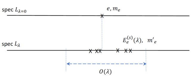
Figure 1: An eigenvalue ee of L0L_{0} splits into eigenvalues Ee(s)(λ)E_{e}^{(s)}\!(\lambda), s=1,,mes=1,\ldots,m_{e}^{\prime}, of LλL_{\lambda}.

We suppose that L0L_{0} has finitely many eigenvalues ee, of finite multiplicity mem_{e}, possibly embedded in continuous spectrum, which can cover parts or all of \mathbb{R}. The set of eigenvalues ee of L0L_{0} is denoted by 0{\mathcal{E}}_{0} and the associated orthogonal eigenprojection is PeP_{e}. We are going to impose a regularity condition (c.f. (A1) below) which implies the following picture for small λ\lambda: All eigenvalues of LλL_{\lambda} lie inside an O(λ)O(\lambda) neighbourhood of 0{\mathcal{E}}_{0}. Moreover, within such a neighbourhood around any given e0e\in{\mathcal{E}}_{0}, either LλL_{\lambda} does not have any eigenvalues for λ0\lambda\neq 0 (we say ee is unstable), or LλL_{\lambda} does have some eigenvalues, with summed multiplicity mem^{\prime}_{e} not exceeding mem_{e} (we say ee is stable if me=mem^{\prime}_{e}=m_{e}, and partially stable if 0<me<me0<m^{\prime}_{e}<m_{e}). In the analytic perturbation theory of isolated eigenvalues, the summed multiplicity mem^{\prime}_{e} would always equal mem_{e}, but for embedded eigenvalues, it is generically strictly less than mem_{e}. Fig. 1 gives a graphical depiction of the situation.

Let us now introduce the assumptions and discuss their meaning. We start with an assumption to simplify the bookkeeping. It is not essential for our method to work and could be removed at the cost of a more cumbersome presentation.

  • (A1)

    For λ0\lambda\neq 0 small enough, all eigenvalues of LλL_{\lambda} are simple.

We call these eigenvalues Ee(s)(λ)E^{(s)}_{e}(\lambda), with s=1,,memes=1,\ldots,m_{e}^{\prime}\leq m_{e}, and

limλ0Ee(s)(λ)=e,s=1,,me.\lim_{\lambda\rightarrow 0}E_{e}^{(s)}(\lambda)=e,\qquad s=1,\ldots,m_{e}^{\prime}. (2.4)

The next assumption is a key characteristic for the physical situation we want to describe. We assume that the reservoir dynamics has a single stationary state and that the coupled dynamics is dissipative on the orthogonal complement of this state.

  • (A2)

    The reservoir dynamics has a unique stationary state ΩRR\Omega_{\rm R}\in{\mathcal{H}}_{\rm R}, that is, KerLR=ΩR{\rm Ker}L_{\rm R}={\mathbb{C}}\Omega_{\rm R}. We denote

    PR=1lS|ΩRΩR|andPR=1lPR.P_{\rm R}=\mathchoice{\rm 1\mskip-4.0mul}{\rm 1\mskip-4.0mul}{\rm 1\mskip-4.5mul}{\rm 1\mskip-5.0mul}_{\rm S}\otimes|\Omega_{\rm R}\rangle\langle\Omega_{\rm R}|\qquad\mbox{and}\qquad P^{\perp}_{\rm R}=\mathchoice{\rm 1\mskip-4.0mul}{\rm 1\mskip-4.0mul}{\rm 1\mskip-4.5mul}{\rm 1\mskip-5.0mul}_{\mathcal{H}}-P_{\rm R}. (2.5)

    On the orthogonal complement the full, coupled dynamics is dissipative in the sense that there exists a λ>0\lambda_{*}>0 and a dense set 𝒟{\mathcal{D}}\subset{\mathcal{H}} such that λ\forall\lambda with 0|λ|<λ0\leq|\lambda|<\lambda_{*} and ϕ,ψ𝒟\forall\phi,\psi\in{\mathcal{D}},

    maxsupz0j2|zjϕ,RzPR(λ)ψ|\displaystyle\max_{0\leq j\leq 2}\sup_{z\in{\mathbb{C}}_{-}}\Big|\partial_{z}^{j}\langle\phi,R_{z}^{P_{\rm R}}(\lambda)\psi\rangle\Big| \displaystyle\leq C1(ϕ,ψ)<,\displaystyle C_{1}(\phi,\psi)<\infty, (2.6)
    supz|λϕ,RzPR(λ)ψ|\displaystyle\sup_{z\in{\mathbb{C}}_{-}}\Big|\partial_{\lambda}\langle\phi,R_{z}^{P_{\rm R}}(\lambda)\psi\rangle\Big| \displaystyle\leq C1(ϕ,ψ)<.\displaystyle C_{1}(\phi,\psi)<\infty. (2.7)

    Here ={z:Imz<0}{\mathbb{C}}_{-}=\{z\in{\mathbb{C}}:{\rm Im}z<0\} is the open lower complex half plane and

    RzPR(λ)=(PRLλPRz)1RanPRR_{z}^{P_{\rm R}}(\lambda)=(P^{\perp}_{\rm R}L_{\lambda}P^{\perp}_{\rm R}-z)^{-1}\upharpoonright_{{\rm Ran}P^{\perp}_{\rm R}}

    is the reduced resolvent. Here, RanPR\upharpoonright_{{\rm Ran}P^{\perp}_{\rm R}} denotes the restriction of an operator to the subspace RanPR{\rm Ran}P^{\perp}_{\rm R}. In (2.6), (2.7), C1C_{1} is well defined (finite) on 𝒟×𝒟{\mathcal{D}}\times{\mathcal{D}}.

Discussion of Assumption (A2).

  • (i)

    The estimate (2.7) is of technical nature, but the estimate (2.6) is key as it implies that the dynamics generated by L¯λPRLλPRRanPR\bar{L}_{\lambda}\equiv P^{\perp}_{\rm R}L_{\lambda}P^{\perp}_{\rm R}\upharpoonright_{{\rm Ran}P^{\perp}_{\rm R}} is dissipative, meaning that limtϕ,eitL¯λψ=0\lim_{t\rightarrow\infty}\langle\phi,e^{{\rm i}t\bar{L}_{\lambda}}\psi\rangle=0. More precisely, it follows from (2.6), with 0j20\leq j\leq 2 replaced by 0jk0\leq j\leq k, that

    |ϕ,eitL¯λψ|C(1+t2)k/2,\big|\langle\phi,e^{{\rm i}t\bar{L}_{\lambda}}\psi\rangle\big|\leq\frac{C}{(1+t^{2})^{k/2}}, (2.8)

    provided (L¯λ+i)ϕ𝒟(\bar{L}_{\lambda}+{\rm i})\phi\in{\mathcal{D}} and (L¯λ+i)ψ𝒟(\bar{L}_{\lambda}+{\rm i})\psi\in{\mathcal{D}}. Specifically, (2.6) implies time decay t2\propto t^{-2} (k=2k=2) of overlaps (2.8). We prove (2.8) at the end of this section.

  • (ii)

    We argue that (2.6) is a natural assumption. Namely, (2.6) for λ=0\lambda=0 is implied by

    maxsupz0j2|zjϕ,(LRz)1PRψR|C1(ϕ,ψ)<,\max_{0\leq j\leq 2}\sup_{z\in{\mathbb{C}}_{-}}\Big|\partial_{z}^{j}\langle\phi,(L_{\rm R}-z)^{-1}P_{\rm R}^{\perp}\psi\rangle_{{\mathcal{H}}_{\rm R}}\Big|\leq C_{1}(\phi,\psi)<\infty, (2.9)

    where we understand here (c.f. (2.5)) PR=|ΩRΩR|P_{\rm R}=|\Omega_{\rm R}\rangle\langle\Omega_{\rm R}|, PR=1lRPRP_{\rm R}^{\perp}=\mathchoice{\rm 1\mskip-4.0mul}{\rm 1\mskip-4.0mul}{\rm 1\mskip-4.5mul}{\rm 1\mskip-5.0mul}_{\rm R}-P_{\rm R}. This is readily seen by writing

    RzPR(0)=(L0z)1PR=e0PS,e(LRez)1PR,R_{z}^{P_{\rm R}}(0)=(L_{0}-z)^{-1}P^{\perp}_{\rm R}=\sum_{e\in{\mathcal{E}}_{0}}P_{{\rm S},e}\otimes(L_{\rm R}-e-z)^{-1}P^{\perp}_{\rm R},

    where PS,eP_{{\rm S},e} is the spectral projection of LSL_{\rm S} associated to ee, so that e0PS,e=1lS\sum_{e\in{\mathcal{E}}_{0}}P_{{\rm S},e}=\mathchoice{\rm 1\mskip-4.0mul}{\rm 1\mskip-4.0mul}{\rm 1\mskip-4.5mul}{\rm 1\mskip-5.0mul}_{\rm S}. In turn, (2.9) is a natural assumption on the dynamics of a reservoir, since that dynamics should be dissipative away from the stationary state. In concrete applications, one starts with (2.6) for λ=0\lambda=0 and then proves its validity for small λ0\lambda\neq 0 by perturbation theory [27].

  • (iii)

    In some recent works on the dynamics on open quantum systems [21, 26], the assumption (2.6) is replaced by the condition that zϕ,RzPR(λ)ψz\mapsto\langle\phi,R^{P_{\rm R}}_{z}(\lambda)\psi\rangle have a meromorphic continuation from zz in the lower complex plane across the real axis into the upper plane. This is a much stronger condition than (2.6). In applications to open quantum systems, this difference means that the reservoir correlation function has to decay exponentially quickly in time for the meromorphic situation, while under the present assumption, the decay only needs to be polynomial, c.f. [27].

  • (iv)

    Without loss of generality, we may assume that C1(ϕ,ψ)=C1(ψ,ϕ)C_{1}(\phi,\psi)=C_{1}(\psi,\phi) and that C1(ϕ,ψ)=C1(PRϕ,PRψ)C_{1}(\phi,\psi)=C_{1}(P^{\perp}_{\rm R}\phi,P^{\perp}_{\rm R}\psi) in (2.6), (2.7).

As is well known (see e.g. Proposition 4.1 of [8]) if AA is a self-adjoint operator and for each vector ϕ\phi in some dense set, there exists a constant C(ϕ)C(\phi) such that

lim infϵ0+supx(a,b)|ϕ,(Ax+iϵ)1ϕ|C(ϕ),\liminf_{\epsilon\rightarrow 0_{+}}\sup_{x\in(a,b)}|\langle\phi,(A-x+{\rm i}\epsilon)^{-1}\phi\rangle|\leq C(\phi),

then the spectrum of AA in the interval (a,b)(a,b) is purely absolutely continuous. Thus the estimate (2.6) with j=0j=0 implies that the spectrum of PRLλPRP^{\perp}_{\rm R}L_{\lambda}P^{\perp}_{\rm R} acting on RanPR{\rm Ran}P_{\rm R}^{\perp} is purely absolutely continuous and for λ=0\lambda=0, this implies that the spectrum of L0L_{0} reduced to RanPR{\rm Ran}P_{\rm R}^{\perp} is purely absolutely continuous. On the finite dimensional part RanPRS{\rm Ran}P_{\rm R}\cong{\mathcal{H}}_{\rm S}, the operator L0L_{0} is (identified with) LSL_{\rm S} which has pure point spectrum 0{\mathcal{E}}_{0}. Therefore L0L_{0} has absolutely continuous spectrum except for the eigenvalues 0{\mathcal{E}}_{0}, the same as those of LSL_{\rm S} and the eigenprojection PeP_{e} of L0L_{0} associated to ee is given by

Pe=(PS,e1lR)PRPS,ePR,P_{e}=(P_{{\rm S},e}\otimes\mathchoice{\rm 1\mskip-4.0mul}{\rm 1\mskip-4.0mul}{\rm 1\mskip-4.5mul}{\rm 1\mskip-5.0mul}_{\rm R})P_{\rm R}\equiv P_{{\rm S},e}\otimes P_{\rm R}, (2.10)

where PS,eP_{{\rm S},e} is the eigenprojection associated to ee as an eigenvalue of LSL_{\rm S}.

2.2 Instability of embedded eigenvalues and how to track them

If ee is an isolated eigenvalue of L0L_{0} then by standard analytic perturbation theory [19] LλL_{\lambda} has eigenvalues Ee(s)(λ)E^{(s)}_{e}(\lambda) close to ee, for λ\lambda small. Those eigenvalues coincide with the eigenvalues of the operator

ePe+λPeIPeλ2PeI(L0e)1PeIPe+O(λ3).eP_{e}+\lambda P_{e}IP_{e}-\lambda^{2}P_{e}I(L_{0}-e)^{-1}P^{\perp}_{e}IP_{e}+O(\lambda^{3}). (2.11)

Each term in the expansion (2.11) is self-adjoint. If ee is an embedded eigenvalue of L0L_{0} then the reduced resolvent (L0e)1Pe(L_{0}-e)^{-1}P^{\perp}_{e} in (2.11) is not defined as a bounded operator. However, its regularization (L0e+iϵ)1Pe(L_{0}-e+{\rm i}\epsilon)^{-1}P^{\perp}_{e} certainly is, for any ϵ>0\epsilon>0. We may hope that in a sense, the perturbation expansion (2.11) stays valid also for embedded eigenvalues, upon regularizing the resolvent and taking ϵ0+\epsilon\rightarrow 0_{+}. But due to the regularization, the operator (L0e+iϵ)1Pe(L_{0}-e+{\rm i}\epsilon)^{-1}P^{\perp}_{e} is not self-adjoint any longer! So according to (2.11), the second order corrections to the embedded eigenvalue would become complex numbers. This is, however, not compatible with LλL_{\lambda} being self-adjoint. We may then intuit that for small nonzero λ\lambda, the number mem_{e}^{\prime} of eigenvalues of LλL_{\lambda} close to ee might be strictly reduced, me<mem_{e}^{\prime}<m_{e}, and that this reduction is accounted for by the existence of complex eigenvalues of the so-called level shift operator

Λe=PeIPe(L0e+i0+)1IPe.\Lambda_{e}=-P_{e}IP^{\perp}_{e}(L_{0}-e+{\rm i}0_{+})^{-1}IP_{e}. (2.12)

Here, (L0e+i0+)1(L_{0}-e+{\rm i}0_{+})^{-1} is the limit of (L0e+iϵ)1(L_{0}-e+{\rm i}\epsilon)^{-1} as ϵ0+\epsilon\rightarrow 0_{+}, taken in the sense of the operator norm in the expression (2.12). This mechanism has the following precise formulation.

Let QQ be an orthogonal projection on \mathcal{H} and set Q=1lQQ^{\perp}=\mathchoice{\rm 1\mskip-4.0mul}{\rm 1\mskip-4.0mul}{\rm 1\mskip-4.5mul}{\rm 1\mskip-5.0mul}-Q. The Feshbach map applied to an operator AA on \mathcal{H} is defined by

𝔉(A;Q)=Q(AAQ(QAQRanQ)1A)Q,{\mathfrak{F}}(A;Q)=Q\big(A-AQ^{\perp}(Q^{\perp}AQ^{\perp}\upharpoonright_{{\rm Ran}Q^{\perp}})^{-1}A\big)Q, (2.13)

where it is assumed that QAQRanQQ^{\perp}AQ^{\perp}\upharpoonright_{{\rm Ran}Q^{\perp}} is invertible. The Feshbach map satisfies the following isospectrality property: Let aa\in\mathbb{C} be in the resolvent set of the operator QAQRanQQ^{\perp}AQ^{\perp}\upharpoonright_{{\rm Ran}Q^{\perp}}, so that 𝔉(Aa,Q){\mathfrak{F}}(A-a;Q) is well defined. Then the isospectrality property says that aa is an eigenvalue of AA if and only if zero is an eigenvalue of 𝔉(Aa,Q){\mathfrak{F}}(A-a;Q). The redeeming quality of this mapping is that 𝔉(Aa,Q){\mathfrak{F}}(A-a;Q) acts on RanQ{\rm Ran}Q, a space smaller than \mathcal{H} (reduction in dimension). Consider now, for zz\in{\mathbb{C}}_{-},

𝔉(Lλz,Pe)=Pe(ez+λIλ2IRzPe(λ)PeI)Pe,{\mathfrak{F}}(L_{\lambda}-z;P_{e})=P_{e}\Big(e-z+\lambda I-\lambda^{2}IR_{z}^{P_{e}}(\lambda)P^{\perp}_{e}I\Big)P_{e}, (2.14)

where RzPe(λ)(PeLλPez)1RanPeR_{z}^{P_{e}}(\lambda)\equiv(P_{e}^{\perp}L_{\lambda}P_{e}^{\perp}-z)^{-1}\upharpoonright_{{\rm Ran}P^{\perp}_{e}} is the reduced resolvent. The isospectrality is not of any good use to analyze the spectrum of LλL_{\lambda} directly, since RzPe(λ)R_{z}^{P_{e}}(\lambda) is not defined for real zz. However, one can show (see Theorem A1 of [20] and also Theorem 4.1 below) that the condition (A2), together with the assumption22 2 In applications, this a very weak assumption: according to (2.10), on the reservoir part, PeP_{e} projects onto the stationary state ΩR\Omega_{\rm R}. This means that the operator II only has to be applicable to vectors in SΩR{\mathcal{H}}_{\rm S}\otimes{\mathbb{C}}\Omega_{\rm R}. In particular, the reservoir part of the interaction II can be an unbounded operator, as long as ΩR\Omega_{\rm R} is in its domain. that

(A3) IPeIP_{e} is a bounded operator and   RanIPe𝒟,\displaystyle{\rm Ran}IP_{e}\subset{\mathcal{D}}, (2.15)

imply that the derivatives of order up to two of

zPeIRzPe(λ)PeIPez\mapsto P_{e}IR_{z}^{P_{e}}(\lambda)P^{\perp}_{e}IP_{e} (2.16)

are bounded uniformly in {z:|Reze|g/2}\{z\in{\mathbb{C}}_{-}:|{\rm Re}z-e|\leq g/2\}. Here,

g=min{|ee|:e,e0,ee}>0g=\min\big\{|e-e^{\prime}|:e,e^{\prime}\in{\mathcal{E}}_{0},\ e\neq e^{\prime}\big\}>0 (2.17)

denotes the minimal gap of the eigenvalues of L0L_{0} (which is the same as that of LSL_{\rm S}). The Feshbach map (2.14) is then well defined (by continuity) for zz\in\mathbb{R}, |ze|g/2|z-e|\leq g/2. Now the isospectrality property can be extended to real values of zz. Namely, one can show (see Theorem 6.1 below and also [11, 3, 20]) that any EE\in{\mathbb{R}} is an eigenvalue of LλL_{\lambda} if and only if zero is an eigenvalue of 𝔉(LλE,Pe){\mathfrak{F}}(L_{\lambda}-E;P_{e}), and that

dimKer(LλE)=dimKer(𝔉(LλE,Pe)).{\rm dim}{\rm Ker}(L_{\lambda}-E)={\rm dim}{\rm Ker}\big({\mathfrak{F}}(L_{\lambda}-E;P_{e})\big). (2.18)

Due to (2.14), eigenvalues of 𝔉(LλE,Pe){\mathfrak{F}}(L_{\lambda}-E;P_{e}) are located in an O(λ)O(\lambda) neighbourhood of 0{\mathcal{E}}_{0}, and hence by isospectrality, so are those of LλL_{\lambda}. The multiplicity of EE as an eigenvalue of LλL_{\lambda} is controlled by (2.18). We assume now

(A4) PeIPe\displaystyle P_{e}IP_{e} =0,\displaystyle=0, (2.19)

as this condition does not alter the emergence of complex eigenvalues (because PeIPeP_{e}IP_{e} is self-adjoint). We could dispense with the condition (2.19) by a simple modification of our arguments. In applications [26, 27, 28], this assumption is naturally satisfied. According to (2.12), (2.14), (2.19),

𝔉(LλE,Pe)=(eE)Pe+λ2Λe+O(λ3).{\mathfrak{F}}(L_{\lambda}-E;P_{e})=(e-E)P_{e}+\lambda^{2}\Lambda_{e}+O(\lambda^{3}). (2.20)

As it acts on the mem_{e}-dimensional space RanPe{\rm Ran}P_{e}, the operator Λe\Lambda_{e} has mem_{e} generally complex eigenvalues. Since Λe\Lambda_{e} it is a dissipative operator, meaning that

ImΛe=limϵ0+PeIϵPe(L0e)2+ϵ2IPe0,{\rm Im}\Lambda_{e}=\lim_{\epsilon\rightarrow 0_{+}}P_{e}I\frac{\epsilon P_{e}^{\perp}}{(L_{0}-e)^{2}+\epsilon^{2}}IP_{e}\,\geq 0, (2.21)

its eigenvalues have non-negative imaginary parts.33 3 It is sometimes useful to note that the real eigenvalues of Λe\Lambda_{e} are automatically semi-simple as they lie on the boundary of the numerical range of Λe\Lambda_{e}, see e.g. Proposition 3.2 of [11]. The isospectrality of the Feshbach map (2.18) and the expansion (2.20) show that for each eigenvalue Ee(s)(λ)E_{e}^{(s)}(\lambda) of LλL_{\lambda}, there is an eigenvalue ae(s)a_{e}^{(s)}\in\mathbb{R} of Λe\Lambda_{e} such that

Ee(s)(λ)=e+λ2ae(s)+O(λ3).E^{(s)}_{e}(\lambda)=e+\lambda^{2}a_{e}^{(s)}+O(\lambda^{3}). (2.22)

However, Λe\Lambda_{e} may have real eigenvalues without LλL_{\lambda} having any eigenvalues close to ee (for λ\lambda small, nonzero). This is so since the O(λ3)O(\lambda^{3}) term in (2.20) may cause the spectrum of (2.20) to be non-real. In this case, LλL_{\lambda} does not have any eigenvalues close to ee, according to (2.18). To simplify the analysis, we do not consider this higher order effect. Instead, we assume that the real eigenvalues of Λe\Lambda_{e} are in bijection with the eigenvalues Ee(s)(λ)E_{e}^{(s)}(\lambda) of LλL_{\lambda} close to ee. One way to ensure this is to impose the condition

(A5) The eigenvalues of Λe\Lambda_{e} are simple and Λe\Lambda_{e} has exactly mem^{\prime}_{e} real eigenvalues.

We recall that mem^{\prime}_{e}, defined before (2.4), is the number of (distinct and simple) eigenvalues of LλL_{\lambda} close to ee, for small λ0\lambda\neq 0. Assuming Λe\Lambda_{e} to have purely simple spectrum is done for convenience of the presentation. This restriction can be removed easily and our approach still works, as long as Λe\Lambda_{e} is diagonalizable. In some models, it can happen though that Λe\Lambda_{e} is not diagonalizable at so-called exceptional points of parameters; one then expects a qualitatively different behaviour of the dynamics (Jordan blocks of Λe\Lambda_{e} cause polynomial corrections to exponential decay in time). We do not further explore this interesting aspect here.

The condition (A5) without the simplicity assumption is also called the Fermi Golden Rule Condition. It ensures that stability or instability of eigenvalues of LλL_{\lambda} is detected at the lowest order (λ2\lambda^{2}) in the perturbation. In terms of dynamical properties, the condition (A5) means that metastable states have life-times of O(λ2)O(\lambda^{-2}), as shown in Theorem 3.1.

2.3 How to link stable and unstable eigenvalues to the dynamics

We have seen above that the (partially) stable eigenvalues of LλL_{\lambda} are the real eigenvalues of the level shift operators Λe\Lambda_{e} and that the Λe\Lambda_{e} may have eigenvalues ae(s)a_{e}^{(s)} with strictly positive imaginary part. We introduced the level shift operators Λe\Lambda_{e} as the second order (λ2)(\lambda^{2}) contributions in the Feshbach map, (2.20). The isospectrality property of the Feshbach map then linked Λe\Lambda_{e} to the spectrum of LλL_{\lambda}. As it turns out, the Feshbach map is also an ingredient in the block decomposition of an operator HH acting on =RanQRanQ{\mathcal{H}}={\rm Ran}Q\oplus{\rm Ran}Q^{\perp}, where QQ is an orthogonal projection. More precisely, one can readily verify that for any operator HH such that 𝔉(H,Q){\mathfrak{F}}(H;Q) exists, the following identity holds (see Section 6, in particular (6.5)),

H=(1lQHQRzQ01l)(𝔉(H,Q)00QHQ)(1l0RzQQHQ1l).H=\begin{pmatrix}\mathchoice{\rm 1\mskip-4.0mul}{\rm 1\mskip-4.0mul}{\rm 1\mskip-4.5mul}{\rm 1\mskip-5.0mul}&QHQ^{\perp}R_{z}^{Q}\\ 0&\mathchoice{\rm 1\mskip-4.0mul}{\rm 1\mskip-4.0mul}{\rm 1\mskip-4.5mul}{\rm 1\mskip-5.0mul}\end{pmatrix}\begin{pmatrix}{\mathfrak{F}}(H;Q)&0\\ 0&Q^{\perp}HQ^{\perp}\end{pmatrix}\begin{pmatrix}\mathchoice{\rm 1\mskip-4.0mul}{\rm 1\mskip-4.0mul}{\rm 1\mskip-4.5mul}{\rm 1\mskip-5.0mul}&0\\ R^{Q}_{z}Q^{\perp}HQ&\mathchoice{\rm 1\mskip-4.0mul}{\rm 1\mskip-4.0mul}{\rm 1\mskip-4.5mul}{\rm 1\mskip-5.0mul}\end{pmatrix}. (2.23)

The first component in the 2×22\times 2 decomposition of (2.23) is that of RanQ{\rm Ran}Q, the second one that of RanQ{\rm Ran}Q^{\perp}. Choosing in (2.23) Q=PeQ=P_{e} and H=LλzH=L_{\lambda}-z for z\z\in{\mathbb{C}}\backslash{\mathbb{R}} gives the decomposition

(Lλz)1=[𝔉(Lλz,Pe)]1+𝔅(z)+RzPe(λ),(L_{\lambda}-z)^{-1}=[{\mathfrak{F}}(L_{\lambda}-z;P_{e})]^{-1}+{\mathfrak{B}}(z)+R_{z}^{P_{e}}(\lambda), (2.24)

where (z){\mathcal{B}}(z) is a term of O(λ)O(\lambda), see (4.3). The first term on the right side is the inverse of the Feshbach map, an operator acting on RanPe{\rm Ran}P_{e} and the last term acts on RanPe{\rm Ran}P_{e}^{\perp}. The resolvent, (2.24), is linked to the propagator via the Fourier-Laplace transform, for w>0w>0,

eitLλ=12πiiweitz(Lλz)1𝑑z.e^{{\rm i}tL_{\lambda}}=\frac{-1}{2\pi{\rm i}}\int_{{\mathbb{R}}-{\rm i}w}e^{{\rm i}tz}(L_{\lambda}-z)^{-1}dz. (2.25)

Using (2.24) in (2.25) provides a link between the Feshbach map and the dynamics. We then expand the (inverse) of the first term on the right side of (2.24), 𝔉(Lλz,Pe)=ez+λ2Λe+O(|λ|3+λ2|ze|){\mathfrak{F}}(L_{\lambda}-z;P_{e})=e-z+\lambda^{2}\Lambda_{e}+O(|\lambda|^{3}+\lambda^{2}|z-e|). For zz close to ee, this links [𝔉(Lλz,Pe)]1[{\mathfrak{F}}(L_{\lambda}-z;P_{e})]^{-1} to (ez+λ2Λe)1(e-z+\lambda^{2}\Lambda_{e})^{-1}, which has poles z=e+λ2ae(s)z=e+\lambda^{2}a_{e}^{(s)} at the eigenvalues of e+λ2Λee+\lambda^{2}\Lambda_{e}. Upon “integration around” those poles, in accordance with (2.25), one can extract the dynamical factors eit(e+λ2ae(s))e^{{\rm i}t(e+\lambda^{2}a_{e}^{(s)})}. This procedure works locally, that is, for zz close to a fixed ee. So we will subdivide the integration contour in (2.25) into regions close to e0e\in{\mathcal{E}}_{0}, for each ee, and apply the Feshbach map with the appropriate PeP_{e}. On the complement, where zz is away from all eigenvalues of L0L_{0}, a similar analysis is done using the Feshbach map with projection PRP_{\rm R}. This is the outline of the idea, and we refer to Section 4 for the detailed analysis.

Proof of (2.8). Let ϕ,ψRanPR\phi,\psi\in{\rm Ran}P_{\rm R}^{\perp} and use the resolvent representation (Cauchy formula or Fourier-Laplace transform),

ϕ,eitL¯λψ=12πiiweitzϕ,RzPR(λ)ψ𝑑z,\langle\phi,e^{{\rm i}t\bar{L}_{\lambda}}\psi\rangle=\frac{-1}{2\pi{\rm i}}\int_{{\mathbb{R}}-{\rm i}w}e^{{\rm i}tz}\langle\phi,R^{P_{\rm R}}_{z}(\lambda)\psi\rangle dz, (2.26)

where w>0w>0 is arbitrary. We have

RzPR(λ)\displaystyle R_{z}^{P_{\rm R}}(\lambda) =\displaystyle= (z+i)1[1l+RzPR(λ)(L¯λ+i)]\displaystyle(z+{\rm i})^{-1}[-\mathchoice{\rm 1\mskip-4.0mul}{\rm 1\mskip-4.0mul}{\rm 1\mskip-4.5mul}{\rm 1\mskip-5.0mul}+R_{z}^{P_{\rm R}}(\lambda)\,(\bar{L}_{\lambda}+{\rm i})] (2.27)
=\displaystyle= (z+i)1(z+i)2(L¯λ+i)+(z+i)2RzPR(λ)(L¯λ+i)2.\displaystyle-(z+{\rm i})^{-1}-(z+{\rm i})^{-2}(\bar{L}_{\lambda}+{\rm i})+(z+{\rm i})^{-2}R_{z}^{P_{\rm R}}(\lambda)\,(\bar{L}_{\lambda}+{\rm i})^{2}.

Since eitx(x+i(1w))k𝑑x=0\int_{\mathbb{R}}\frac{e^{{\rm i}tx}}{(x+{\rm i}(1-w))^{k}}dx=0 for t>0t>0 and w<1w<1, the relations (2.26) and (2.27) imply

ϕ,eitL¯λψ=12πiiweitz(z+i)2(L¯λ+i)ϕ,RzPR(λ)(L¯λ+i)ψ𝑑z,\langle\phi,e^{{\rm i}t\bar{L}_{\lambda}}\psi\rangle=\frac{-1}{2\pi{\rm i}}\int_{{\mathbb{R}}-{\rm i}w}\frac{e^{{\rm i}tz}}{(z+{\rm i})^{2}}\langle(\bar{L}_{\lambda}+{\rm i})\phi,R^{P_{\rm R}}_{z}(\lambda)(\bar{L}_{\lambda}+{\rm i})\psi\rangle dz, (2.28)

for ϕ,ψDom(L¯λ)\phi,\psi\in{\rm Dom}(\bar{L}_{\lambda}). We now use eitz=(it)1zeitze^{{\rm i}tz}=({\rm i}t)^{-1}\partial_{z}e^{{\rm i}tz} and integrate in (2.28) by parts kk times,

ϕ,eitLλψ\displaystyle\langle\phi,e^{{\rm i}tL_{\lambda}}\psi\rangle =\displaystyle= 1(it)k12πiiweitzzk{(z+i)2(L¯λ+i)ϕ,RzPR(λ)(L¯λ+i)ψ}𝑑z.\displaystyle\frac{1}{({\rm i}t)^{k}}\frac{-1}{2\pi{\rm i}}\int_{{\mathbb{R}}-{\rm i}w}e^{{\rm i}tz}\partial^{k}_{z}\big\{(z+{\rm i})^{-2}\langle(\bar{L}_{\lambda}+{\rm i})\phi,R_{z}^{P_{\rm R}}(\lambda)(\bar{L}_{\lambda}+{\rm i})\psi\rangle\big\}dz.\qquad (2.29)

It now follows from (2.29) and (2.6), with 0j20\leq j\leq 2 replaced by 0jk0\leq j\leq k, that

|ϕ,eitL¯λψ|C1((L¯λ+i)ϕ,(L¯λ+i)ψ)(1+t2)k/2,\big|\langle\phi,e^{{\rm i}t\bar{L}_{\lambda}}\psi\rangle\big|\leq\frac{C_{1}\big((\bar{L}_{\lambda}+{\rm i})\phi,(\bar{L}_{\lambda}+{\rm i})\psi\big)}{(1+t^{2})^{k/2}}, (2.30)

provided (L¯λ+i)ϕ𝒟(\bar{L}_{\lambda}+{\rm i})\phi\in{\mathcal{D}} and (L¯λ+i)ϕ𝒟(\bar{L}_{\lambda}+{\rm i})\phi\in{\mathcal{D}}. In this way, smoothness of the resolvent gives rise to dissipation in the dynamics. This proves (2.8).

3 Main result

Our main result is Theorem 3.1 below. It involves a reduced system dynamics eitM(λ)e^{{\rm i}tM(\lambda)}, and we explain the generator M(λ)M(\lambda) now. The simplicity of the spectrum assumed in (A5) implies that the level shift operators Λe\Lambda_{e} is diagonalizable,

Λe=s=1meae(s)Qe(s).\Lambda_{e}=\sum_{s=1}^{m_{e}}a_{e}^{(s)}Q_{e}^{(s)}. (3.1)

The ae(s)a_{e}^{(s)} are the eigenvalues and the Qe(s)Q_{e}^{(s)} are the rank-one spectral projections, satisfying the disjointness and completeness relations

Qe(s)Qe(s)=Qe(s)δs,sδe,e ands=1meQe(s)=Pe.Q_{e}^{(s)}Q_{e^{\prime}}^{(s^{\prime})}=Q_{e}^{(s)}\delta_{s,s^{\prime}}\delta_{e,e^{\prime}}\quad\mbox{ and}\quad\sum_{s=1}^{m_{e}}Q_{e}^{(s)}=P_{e}.

Given an eigenvalue e0e\in{\mathcal{E}}_{0} of L0L_{0}, we partition the indices s=1,,mes=1,\ldots,m_{e} into the oscillating and decaying classes

𝒮eosc={s:ae(s)}and𝒮edec={s:Imae(s)>0}.{\mathcal{S}}_{e}^{\rm osc}=\big\{s:a_{e}^{(s)}\in{\mathbb{R}}\big\}\qquad\mbox{and}\qquad{\mathcal{S}}_{e}^{\rm dec}=\big\{s:{\rm Im}a_{e}^{(s)}>0\big\}. (3.2)

We define the operators

M(λ)=e0Me,Me=s𝒮edec(e+λ2ae(s))Qe(s)+s𝒮eoscEe(s)(λ)Qe(s).M(\lambda)=\bigoplus_{e\in{\mathcal{E}}_{0}}M_{e},\qquad M_{e}=\sum_{s\in{\mathcal{S}}_{e}^{\rm dec}}\big(e+\lambda^{2}a_{e}^{(s)}\big)Q_{e}^{(s)}+\sum_{s\in{\mathcal{S}}^{\rm osc}_{e}}E_{e}^{(s)}(\lambda)Q_{e}^{(s)}. (3.3)

Since Qe(s)=Qe(s)PR=PRQe(s)Q_{e}^{(s)}=Q_{e}^{(s)}P_{\rm R}=P_{\rm R}Q_{e}^{(s)} we view each MeM_{e} as an operator on RanPS,e{\rm Ran}P_{{\rm S},e}, the eigenspace of LSL_{\rm S} associated to the eigenvalue ee. The operator M(λ)M(\lambda) is then also an operator acting on the system Hilbert space S{\mathcal{H}}_{\rm S} alone. By construction, M(λ)M(\lambda) and LSL_{\rm S} commute, and M(0)=LSM(0)=L_{\rm S}.

Theorem 3.1 (Resonance expansion of propagator)

There is a constant c0>0c_{0}>0 such that if 0<|λ|<c00<|\lambda|<c_{0}, then we have weakly on 𝒟{\mathcal{D}},

eitLλ=eitM(λ)PR+PReitPRLλPRPR+R(λ,t),e^{{\rm i}tL_{\lambda}}=e^{{\rm i}tM(\lambda)}\otimes P_{\rm R}+P^{\perp}_{\rm R}e^{{\rm i}tP^{\perp}_{\rm R}L_{\lambda}P^{\perp}_{\rm R}}P^{\perp}_{\rm R}+R(\lambda,t), (3.4)

where the operator R(λ,t)R(\lambda,t) satisfies

|ϕ,R(λ,t)ψ|C|λ|1/4K(ϕ,ψ),ϕ,ψ𝒟,\big|\langle\phi,R(\lambda,t)\psi\rangle\big|\leq C|\lambda|^{1/4}\,K(\phi,\psi),\qquad\forall\phi,\psi\in{\mathcal{D}}, (3.5)

for constants CC and KK independent of t0t\geq 0.

If interested in ϕ,eitLλψ\langle\phi,e^{-{\rm i}tL_{\lambda}}\psi\rangle, t0t\geq 0, then it suffices to take the adjoint of (3.4). The choice of the sign in the exponent on the left side of (3.4) is motivated by the application of our result to the reduced system dynamics, [27]. The generator M(λ)M(\lambda) is defined in its diagonalized form (3.3) and so eitM(λ)e^{{\rm i}tM(\lambda)} is easily obtained from the functional calculus: The equality (3.4) means that for all ϕ,ψ𝒟\phi,\psi\in{\mathcal{D}},

ϕ,eitLλψ\displaystyle\langle\phi,e^{{\rm i}tL_{\lambda}}\psi\rangle =\displaystyle= e0[s𝒮edeceit(e+λ2ae(s))ϕ,Qe(s)ψ+s𝒮eosceitEe(s)(λ)ϕ,Qe(s)ψ]\displaystyle\sum_{e\in{\mathcal{E}}_{0}}\Big[\sum_{s\in{\mathcal{S}}_{e}^{\rm dec}}e^{{\rm i}t(e+\lambda^{2}a_{e}^{(s)})}\big\langle\phi,Q_{e}^{(s)}\psi\big\rangle+\sum_{s\in{\mathcal{S}}_{e}^{\rm osc}}\,e^{{\rm i}tE_{e}^{(s)}(\lambda)}\big\langle\phi,Q_{e}^{(s)}\psi\big\rangle\Big] (3.6)
+ϕ,PReitPRLλPRPRψ+ϕ,R(λ,t)ψ.\displaystyle+\langle\phi,P^{\perp}_{\rm R}e^{{\rm i}tP^{\perp}_{\rm R}L_{\lambda}P^{\perp}_{\rm R}}P^{\perp}_{\rm R}\psi\rangle+\langle\phi,R(\lambda,t)\psi\rangle.

Discussion of Theorem 3.1

  • (i)

    The operator M(λ)M(\lambda) generally contains all orders of λ\lambda in the oscillatory parts Ee(s)(λ)E_{e}^{(s)}(\lambda), see (3.3). It is clear that we need to include the exact phases (eigenvalues Ee(s)(λ)E_{e}^{(s)}(\lambda) of LλL_{\lambda} to all orders in λ\lambda) in the approximate dynamics on the right side of (3.4), for otherwise we have diverging phase differences, and we cannot get an approximation small in λ\lambda for all times. However, in the decaying terms, we can truncate the exponents at the second order in λ\lambda, keeping only e+λ2ae(s)e+\lambda^{2}a_{e}^{(s)}, and the time decay still allows us a control uniform in tt.

  • (ii)

    On the finite-dimensional part, the dynamics eitM(λ)PRe^{{\rm i}tM(\lambda)}\otimes P_{\rm R} on the right side of (3.4), there are terms oscillating in time, eitEe(s)(λ)\propto e^{{\rm i}tE_{e}^{(s)}(\lambda)}, and terms decaying in time, eit(e+λ2ae(s))\propto e^{{\rm i}t(e+\lambda^{2}a_{e}^{(s)})}. The decay is exponential, with rates λ2Imae(s)>0\lambda^{2}{\rm Im}a_{e}^{(s)}>0, since |eit(e+λ2ae(s))|=eλ2tImae(s)|e^{{\rm i}t(e+\lambda^{2}a_{e}^{(s)})}|=e^{-\lambda^{2}t{\rm Im}a_{e}^{(s)}}. On the infinite-dimensional part (i.e., on RanPR{\rm Ran}P_{\rm R}^{\perp}), the dynamics is also decaying, but only at a polynomial rate 1/t21/t^{2}, as per (2.8).

  • (iii)

    The asymptotic dynamics for times larger than all the life times (λ2Imae(s))1(\lambda^{2}{\rm Im}a_{e}^{(s)})^{-1} and large enough so that the dissipative term ϕ,PReitPRLλPRPRψt2\langle\phi,P^{\perp}_{\rm R}e^{{\rm i}tP^{\perp}_{\rm R}L_{\lambda}P^{\perp}_{\rm R}}P^{\perp}_{\rm R}\psi\rangle\sim t^{-2} has decayed (c.f. (2.8)), is given by eitLλeitM(λ)PRe^{{\rm i}tL_{\lambda}}\approx e^{{\rm i}tM(\lambda)}\otimes P_{\rm R}. If Ee(s)(λ)=0E_{e}^{(s)}(\lambda)=0 is the only eigenvalue of LλL_{\lambda}, then the dynamics relaxes to the final state Qe(s)PRQ_{e}^{(s)}\otimes P_{\rm R} modulo an error O(|λ|1/4)O(|\lambda|^{1/4}).

  • (iv)

    We may call eitM(λ)PRe^{{\rm i}tM(\lambda)}\otimes P_{\rm R} and PReitPRLλPRPRP^{\perp}_{\rm R}e^{{\rm i}tP^{\perp}_{\rm R}L_{\lambda}P^{\perp}_{\rm R}}P^{\perp}_{\rm R} of (3.4) the quasi-static and dissipative parts, respectively. The decomposition (3.4) is reminiscent of the structure of solutions of dispersive partial differential equations, which split into a dispersive wave plus a part converging towards an invariant manifold [34, 39]. In our case, after the decay of the dissipative term, the dynamics first approaches the quasi-static manifold spanned by the Qe(s)Q_{e}^{(s)} for all e,se,s. The orbits stay close to the quasi-static manifold for times up to 1/λ2\sim 1/\lambda^{2}, after which the dynamics moves to the final, invariant manifold spanned, modulo O(|λ|1/4)O(|\lambda|^{1/4}), by the Qe(s)PRQ_{e}^{(s)}\otimes P_{\rm R} with e0e\in{\mathcal{E}}_{0} and s𝒮eoscs\in{\mathcal{S}}_{e}^{\rm osc}.

  • (v)

    The approach we take to prove Theorem 3.1 is similar to [20]. In that paper, an expansion of the dynamics was given as a sum of a main part plus a remainder, similar to (3.4). The remainder of [20] converges to zero in the limit of large times, but it is not shown to be small in λ\lambda. In the current work, the remainder is small in λ\lambda for all times (3.5), but it does not converge to zero for large times. This means, incidentally, that the main term of the current work has a simpler form than the one of [20]. Indeed, the current main term is a second order approximation along the decaying terms, with s𝒮decs\in{\mathcal{S}_{\rm dec}}, of that of [20]. The result of [20] is not suitable for proving the validity of the Markovian approximation, but the current result here is.

Uncorrelated initial states. For vectors of the form ψ=ψSΩR\psi=\psi_{\rm S}\otimes\Omega_{\rm R}, ϕ=ϕSΩR\phi=\phi_{\rm S}\otimes\Omega_{\rm R} the state-dependent constant KK in the remainder (3.5), satisfies K(ϕ,ψ)=ϕSψSK(\phi,\psi)=\|\phi_{\rm S}\|\,\|\psi_{\rm S}\| (see (3.15) below). The term ϕ,PReitPRLλPRPRψ\langle\phi,P^{\perp}_{\rm R}e^{{\rm i}tP^{\perp}_{\rm R}L_{\lambda}P^{\perp}_{\rm R}}P^{\perp}_{\rm R}\psi\rangle vanishes. We then obtain the following result directly from (3.4).

Corollary 3.2

There is a constant c0c_{0} such that if 0<|λ|<c00<|\lambda|<c_{0}, then for all ψS,ϕSS\psi_{\rm S},\phi_{\rm S}\in{\mathcal{H}}_{\rm S}, t0t\geq 0,

|ϕSΩR,eitLλψSΩRSRϕS,eitM(λ)ψSS|C|λ|1/4ϕSψS.\Big|\langle\phi_{\rm S}\otimes\Omega_{\rm R},e^{{\rm i}tL_{\lambda}}\psi_{\rm S}\otimes\Omega_{\rm R}\rangle_{{\mathcal{H}}_{\rm S}\otimes{\mathcal{H}}_{\rm R}}-\langle\phi_{\rm S},e^{{\rm i}tM(\lambda)}\psi_{\rm S}\rangle_{{\mathcal{H}}_{\rm S}}\Big|\leq C|\lambda|^{1/4}\,\|\phi_{\rm S}\|\,\|\psi_{\rm S}\|. (3.7)

This corollary is the starting point for a proof that the Markovian approximation is valid for all times, which we give in [27]. We show that M(λ)M(\lambda) gives rise to a completely positive trace-preserving semigroup acting on system density matrices, which coincides with the well-known Gorini-Kossakovski-Sudarshan-Lindblad semigroup [1, 6, 26]. We point out, though, that correlated intitial states are also treatable with our method – indeed, the main result, Theorem 3.1, does not make an assumption on intital SR{\rm S}{\rm R} correlations. We explore this in [28] (see also Section 1.4).

Parameter dependence. We take some care in estimating c0c_{0}, CC and KK appearing in Theorem 3.1 and Corollary 3.2 in terms of various parameters, as we explain now. The analysis is based on a perturbation theory (λ\lambda small) and the corrections of the spectrum are governed by the level shift operators Λe\Lambda_{e}, whose spectral decomposition is given in (3.1). To quantify the perturbation theory, we introduce the quantities

a\displaystyle a =\displaystyle= mine,s{Imae(s):ae(s)}(smallest nonzero imaginary part)\displaystyle\min_{e,s}\big\{{\rm Im}a_{e}^{(s)}:a_{e}^{(s)}\not\in{\mathbb{R}}\big\}\qquad\mbox{(smallest nonzero imaginary part)} (3.8)
α\displaystyle\alpha =\displaystyle= maxe,s|ae(s)|=maxespr(Λe)(maximal spectral radius)\displaystyle\max_{e,s}|a_{e}^{(s)}|=\max_{e}{\rm spr}(\Lambda_{e})\qquad\mbox{(maximal spectral radius)} (3.9)
δ\displaystyle\delta =\displaystyle= mine,s,s{|ae(s)ae(s)|:ss}(gap in spectrum of the Λe)\displaystyle\min_{e,s,s^{\prime}}\big\{|a_{e}^{(s)}-a_{e}^{(s^{\prime})}|:s\neq s^{\prime}\big\}\qquad\mbox{(gap in spectrum of the $\Lambda_{e}$)} (3.10)
κ\displaystyle\kappa =\displaystyle= maxe,sQe(s)(size of biggest spectral projection)\displaystyle\max_{e,s}\|Q_{e}^{(s)}\|\qquad\mbox{(size of biggest spectral projection)} (3.11)

We also define

ϰ1=maxm,nC1(I(φmΩR),I(φnΩR)),\varkappa_{1}=\max_{m,n}C_{1}\big(I(\varphi_{m}\otimes\Omega_{\rm R}),I(\varphi_{n}\otimes\Omega_{\rm R})\big), (3.12)

where C1(,)C_{1}(\cdot,\cdot) is given in (2.6) and where {φm}m=1dimS\{\varphi_{m}\}_{m=1}^{\dim{\mathcal{H}}_{\rm S}} is an orthonormal eigenbasis of LSL_{\rm S}. The parameter ϰ1\varkappa_{1} is well defined since due to (2.15), the vectors IφmΩRI\varphi_{m}\otimes\Omega_{\rm R} are in 𝒟\mathcal{D}. We combine all these constants and the spectral gap gg of L0L_{0} (see (2.17)) into the following two effective constants,

ϰ0\displaystyle\varkappa_{0} =\displaystyle= max[1,1/g,κ/a,ακ,ϰ1(1+ϰ1)(1+g+1/g),\displaystyle\max\Big[1,1/g,\kappa/a,\alpha\kappa,\varkappa_{1}(1+\varkappa_{1})(1+g+1/g), (3.13)
ϰ1(1+ϰ14)κmax{1,1+αδ,1/a,1+κaδ,κ2(κa(1+κ3/δ3)(1+1/a)+1/δ2)}]\displaystyle\varkappa_{1}(1+\varkappa_{1}^{4})\kappa\max\big\{1,\tfrac{1+\alpha}{\delta},1/a,\tfrac{1+\kappa}{a\delta},\kappa^{2}\big(\tfrac{\kappa}{a}(1+\kappa^{3}/\delta^{3})(1+1/a)+1/\delta^{2}\big)\big\}\Big]\qquad
λ0\displaystyle\lambda_{0} =\displaystyle= min[1,a,δ/κ2,IPR,g3/2]max[1,ϰ1κ(1+ϰ1κ/δ),α,ϰ1].\displaystyle\frac{\min\Big[1,a,\delta/\kappa^{2},\|IP_{\rm R}\|,g^{3/2}\Big]}{\max\Big[1,\varkappa_{1}\kappa(1+\varkappa_{1}\kappa/\delta),\alpha,\varkappa_{1}\Big]}. (3.14)

Furthermore, for vectors ϕ,ψ𝒟\phi,\psi\in{\mathcal{D}} such that L¯λϕ,L¯λϕ𝒟\bar{L}_{\lambda}\phi,\bar{L}_{\lambda}\phi\in{\mathcal{D}}, with L¯λ=PRLλPR\bar{L}_{\lambda}=P^{\perp}_{\rm R}L_{\lambda}P^{\perp}_{\rm R}, we define

K(ϕ,ψ)\displaystyle K(\phi,\psi) =\displaystyle= ϕψ+maxj=1,2Cj(ϕ,ψ)\displaystyle\|\phi\|\,\|\psi\|+\max_{j=1,2}C_{j}(\phi,\psi) (3.15)
+maxj=1,2(maxmCj(IφmΩR,ϕ)maxmCj(IφmΩR,ψ))\displaystyle+\max_{j=1,2}\big(\max_{m}C_{j}(I\varphi_{m}\otimes\Omega_{\rm R},\phi)\max_{m}C_{j}(I\varphi_{m}\otimes\Omega_{\rm R},\psi)\big)
+𝔖ϕψϕmaxj,mCj(IφmΩR,ψ)\displaystyle+{\mathfrak{S}}_{\phi\leftrightarrow\psi}\|\phi\|\max_{j,m}C_{j}(I\varphi_{m}\otimes\Omega_{\rm R},\psi)
+𝔖ϕψ(ϕ+maxmC1(IφmΩR,ϕ))\displaystyle+{\mathfrak{S}}_{\phi\leftrightarrow\psi}\Big(\|\phi\|+\max_{m}C_{1}(I\varphi_{m}\otimes\Omega_{\rm R},\phi)\Big)
×(PRIPRψ+maxmC1(IφmΩR,(L¯λ+i)PRψ)).\displaystyle\quad\times\Big(\|P_{\rm R}I\|\|P^{\perp}_{\rm R}\psi\|+\max_{m}C_{1}\big(I\varphi_{m}\otimes\Omega_{\rm R},(\bar{L}_{\lambda}+{\rm i})P^{\perp}_{\rm R}\psi\big)\Big).

In (3.15) we use the notation

𝔖ϕψE(ϕ,ψ)=E(ϕ,ψ)+E(ψ,ϕ){\mathfrak{S}}_{\phi\leftrightarrow\psi}E(\phi,\psi)=E(\phi,\psi)+E(\psi,\phi) (3.16)

for any function EE of ϕ\phi and ψ\psi.

Proposition 3.3 (Parameter dependence of c0,C,Kc_{0},C,K)

The constants c0,Cc_{0},C of Theorem 3.1 and Corollary 3.2 can be written as c0=cλ04/3c_{0}=c^{\prime}\lambda_{0}^{4/3} and C=Cϰ0C=C^{\prime}\varkappa_{0}, where c,Cc^{\prime},C^{\prime} do not depend on λ,g,a,α,κ,δ\lambda,g,a,\alpha,\kappa,\delta and λ0\lambda_{0}, ϰ0\varkappa_{0} are given in (3.14) and (3.13), respectively. The constant KK in (3.5), which is a function on 𝒟×𝒟{\mathcal{D}}\times{\mathcal{D}}, is given by (3.15).

Remark. The parameter ϰ1\varkappa_{1}, (3.12), is defined in terms of the function C1C_{1}, (2.6). The latter describes the dissipative nature of the interacting dynamics and, a priori, depends on λ\lambda. However, the dissipation is due to the nature of the environment alone and so in applications, one can bound ϰ1\varkappa_{1} uniformly in λ\lambda, for small enough λ\lambda (see [27]). See also the point (ii) in the discussion of condition (A2) above. In this sense, ϰ1\varkappa_{1} and thus λ0\lambda_{0}, are independent of λ\lambda.

4 Proof of Theorem 3.1

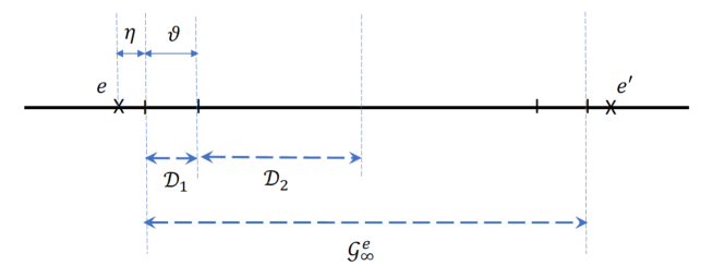
We are presenting the core strategy in Section 4.1. It involves estimates which we derive in Sections 4.3 and 4.4. We then collect the estimates and implement the outlined strategy in Section 4.5. As we explained after Theorem 3.1, our approach is similar to that of [20]. However, in order to be able to show that the remainder is small in λ\lambda for all times, (3.5), we need to substantially modify the analysis of [20]. The main alteration is the introduction of two new energy scales η\eta and ϑ\vartheta which allow for a more detailed estimation of the resolvent. See also Fig. 2 and Fig. 4.

Notational convention. For X,Y0X,Y\geq 0, we write XYX\prec Y to mean that there is a constant CC independent of the coupling constant λ\lambda as well as the parameters g,a,α,δ,κg,a,\alpha,\delta,\kappa, such that XCYX\leq CY. (Recall the definitions (2.17), (3.8)-(3.11) of those parameters.)

4.1 Strategy

Given an orthogonal projection QQ on {\mathcal{H}} we set Q=1lQQ^{\perp}=\mathchoice{\rm 1\mskip-4.0mul}{\rm 1\mskip-4.0mul}{\rm 1\mskip-4.5mul}{\rm 1\mskip-5.0mul}-Q and we denote the resolvent and reduced resolvent operators by

Rz(λ)=(Lλz)1andRzQ(λ)=(QLλQz)1RanQ.R_{z}(\lambda)=(L_{\lambda}-z)^{-1}\qquad\mbox{and}\qquad R_{z}^{Q}(\lambda)=(Q^{\perp}L_{\lambda}Q^{\perp}-z)^{-1}\upharpoonright_{{\rm Ran}Q^{\perp}}. (4.1)

The resolvent representation of the propagator is

ϕ,eitLψ=12πiiweitzϕRz(λ)ψ𝑑z,\langle\phi,\,e^{{\rm i}tL}\psi\rangle=\frac{-1}{2\pi{\rm i}}\int_{{\mathbb{R}}-{\rm i}w}e^{{\rm i}tz}\langle\phi\,R_{z}(\lambda)\psi\rangle\,dz, (4.2)

valid for any w>0w>0 if either of ψ\psi or ϕ\phi belong to Dom(L){\rm Dom}(L) (see [14]). Given an orthogonal projection QQ, the resolvent has a decomposition into a sum of three parts:44 4 Reminiscent of “… est omnis divisa in partes tres …”, [7] a part acting on RanQ{\rm Ran}Q, one acting on RanQ{\rm Ran}Q^{\perp} and one part mixing these subspaces. This decomposition reads, for z\z\in{\mathbb{C}}\backslash{\mathbb{R}},

Rz(λ)=𝔉(z)1+𝔅(z)+RzQ(λ).R_{z}(\lambda)={\mathfrak{F}}(z)^{-1}+{\mathfrak{B}}(z)+R^{Q}_{z}(\lambda). (4.3)

Here, 𝔉\mathfrak{F} is the Feshbach map (2.13),

𝔉(z)𝔉(Lz,Q)=Q(LzLQRzQ(λ)L)Q.{\mathfrak{F}}(z)\equiv{\mathfrak{F}}(L-z;Q)=Q(L-z-LQ^{\perp}R_{z}^{Q}(\lambda)L)Q. (4.4)

The operator 𝔅(z){\mathfrak{B}}(z) in (4.3) is given by

𝔅(z)=𝔉(z)1QLRzQRzQLQ𝔉(z)1+RzQLQ𝔉(z)1QLRzQ.{\mathfrak{B}}(z)=-{\mathfrak{F}}(z)^{-1}QLR_{z}^{Q}-R_{z}^{Q}LQ{\mathfrak{F}}(z)^{-1}+R^{Q}_{z}LQ{\mathfrak{F}}(z)^{-1}QLR_{z}^{Q}. (4.5)

Here and in what follows, it is convenient to simply write RzQR_{z}^{Q} for RzQ(λ)R_{z}^{Q}(\lambda). The existence of 𝔉(z)1{\mathfrak{F}}(z)^{-1} is automatic, this operator equals QRz(λ)QQR_{z}(\lambda)Q, see (4.3). It is elementary to establish the relation (4.3), see Section 6 for more detail.

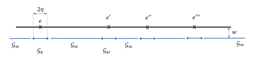
Our strategy is to partition the integration contour iw{\mathbb{R}}-{\rm i}w in (4.2) into segments, see Fig. 2, and apply (4.3) with suitable projections QQ on each segment. To describe the partition, fix an η>0\eta>0. It will be chosen as a certain positive power of |λ||\lambda| later on, so η\eta is a small parameter (relative to the eigenvalue gap gg of L0L_{0}, (2.17)). For every eigenvalue ee of L0L_{0} define the segment (see Fig. ​2)

𝒢e={xiw:|xe|η}and set𝒢={xiw:dist(x,0)>η},{\mathcal{G}}_{e}=\big\{x-{\rm i}w\ :\ |x-e|\leq\eta\big\}\quad\mbox{and set}\quad{\mathcal{G}}_{\infty}=\big\{x-{\rm i}w\ :\ {\rm dist}(x,{\mathcal{E}}_{0})>\eta\big\}, (4.6)

where w>0w>0 is the parameter in (4.2) and 0{\mathcal{E}}_{0} is the set of all eigenvalues of L0L_{0}.

Refer to caption
Figure 2: Subdivision of the integration path iw{\mathbb{R}}-{\rm i}w.

We have the disjoint decomposition iw=𝒢e0𝒢e{\mathbb{R}}-{\rm i}w={\mathcal{G}}_{\infty}\bigcup_{e\in{\mathcal{E}}_{0}}{\mathcal{G}}_{e} and (4.2) gives

ϕ,eitLλψ=e0Je(t)+J(t),withJ#(t)=12πi𝒢#eitzϕ,Rzψ𝑑z.\langle\phi,e^{{\rm i}tL_{\lambda}}\psi\rangle=\sum_{e\in{\mathcal{E}}_{0}}J_{e}(t)+J_{\infty}(t),\quad\mbox{with}\quad J_{\#}(t)=\frac{-1}{2\pi{\rm i}}\int_{{\mathcal{G}}_{\#}}e^{{\rm i}tz}\langle\phi,\,R_{z}\,\psi\rangle\,dz. (4.7)

On 𝒢e{\mathcal{G}}_{e} we will apply the Feshbach map with projection Q=PeQ=P_{e}, (2.10), and on 𝒢{\mathcal{G}}_{\infty} we use the projection Q=PRQ=P_{\rm R}, (2.5). Accordingly, it is important that we have dissipative bounds on the reduced resolvents, i.e., the following local limiting absorption principles, which follow from the global ones given in (2.6), (2.7).

Theorem 4.1 (Local limiting absorption principle)

If λ2ϰ1g\lambda^{2}\varkappa_{1}\prec g then we have for all ϕ,ψ𝒟\phi,\psi\in{\mathcal{D}} and all e0e\in{\mathcal{E}}_{0}

max0j2sup{z:|ze|g/2}|zjϕ,RzPe(λ)ψ|\displaystyle\max_{0\leq j\leq 2}\sup_{\{z\in{\mathbb{C}}_{-}\,:\,|z-e|\leq g/2\}}\Big|\partial_{z}^{j}\langle\phi,R_{z}^{P_{e}}(\lambda)\psi\rangle\Big| \displaystyle\leq C2(ϕ,ψ)<,\displaystyle C_{2}(\phi,\psi)<\infty, (4.8)
sup{z:|ze|g/2}|λϕ,RzPe(λ)ψ|\displaystyle\sup_{\{z\in{\mathbb{C}}_{-}\,:\,|z-e|\leq g/2\}}\Big|\partial_{\lambda}\langle\phi,R_{z}^{P_{e}}(\lambda)\psi\rangle\Big| \displaystyle\leq C2(ϕ,ψ)<,\displaystyle C_{2}(\phi,\psi)<\infty, (4.9)

where C2(,)C_{2}(\cdot,\cdot) is well defined (finite) on 𝒟×𝒟{\mathcal{D}}\times{\mathcal{D}} and satisfies

C2(ϕ,ψ)C1(ϕ,ψ)+max{1,1/g3}[ϕψ\displaystyle C_{2}(\phi,\psi)\prec C_{1}(\phi,\psi)+\max\{1,1/g^{3}\}\Big[\|\phi\|\,\|\psi\| (4.10)
+λ2maxmC1(ϕ,IφmΩR)C1(ψ,IφmΩR)+|λ|𝔖ϕψψmaxmC1(ϕ,IφmΩR)].\displaystyle+\lambda^{2}\max_{m}C_{1}(\phi,I\varphi_{m}\otimes\Omega_{\rm R})C_{1}(\psi,I\varphi_{m}\otimes\Omega_{\rm R})+|\lambda|{\mathfrak{S}}_{\phi\leftrightarrow\psi}\|\psi\|\max_{m}C_{1}(\phi,I\varphi_{m}\otimes\Omega_{\rm R})\Big].

Furthermore, we have

max0k2sup{z:|Reze|g/2e}|zkϕ,RzPRψ|C2(ϕ,ψ).\max_{0\leq k\leq 2}\sup_{\{z\in{\mathbb{C}}_{-}\,:\,|{\rm Re}z-e|\geq g/2\ \forall e\}}\ \big|\partial_{z}^{k}\langle\phi,R_{z}^{P_{\rm R}}\psi\rangle\big|\leq C_{2}(\phi,\psi). (4.11)

We give a proof of Theorem 4.1 in Section 5.1.1. Similar to ϰ1\varkappa_{1} defined in (3.12), we set

ϰ2=maxm,nC2(I(φmΩR),I(φnΩR)).\varkappa_{2}=\max_{m,n}C_{2}\big(I(\varphi_{m}\otimes\Omega_{\rm R}),I(\varphi_{n}\otimes\Omega_{\rm R})\big). (4.12)

Using (4.10) we get the majorization

ϰ2ϰ1+max{1,1/g3}(|λ|ϰ1+IPR)2.\varkappa_{2}\prec\varkappa_{1}+\max\{1,1/g^{3}\}\big(|\lambda|\varkappa_{1}+\|IP_{\rm R}\|\big)^{2}. (4.13)

Furthermore, imposing the constraints

|λ|ϰ1IPRandλ2ϰ1min{1,g3}|\lambda|\varkappa_{1}\prec\|IP_{\rm R}\|\quad\mbox{and}\quad\lambda^{2}\varkappa_{1}\prec\min\{1,g^{3}\} (4.14)

gives from (4.13) the simple bound,

ϰ2ϰ1.\varkappa_{2}\prec\varkappa_{1}. (4.15)

4.2 Cheat sheet

We keep track of several constants during the estimates to follow. The following cheat sheet is presented for the convenience of the reader.

Symbol Meaning Definition
aa smallest nonzero imaginary part of all Λe\Lambda_{e} (3.8)
ae(s)a_{e}^{(s)} eigenvalues of Λe\Lambda_{e} (3.1)
α\alpha maximal spectral radius of all Λe\Lambda_{e} (3.9)
β\beta inverse temperature
C1(ϕ,ψ)C_{1}(\phi,\psi), C2(ϕ,ψ)C_{2}(\phi,\psi) global, local limiting absorption constants (2.6), (4.8)
δ\delta minimal gap of all Λe\Lambda_{e} (3.10)
ee eigenvalues of LSL_{\rm S} (or L0L_{0}) after (2.2)
η\eta integration domain parameter (4.6)
gg gap of LSL_{\rm S} (2.17)
𝒢e{\mathcal{G}}_{e}, 𝒢{\mathcal{G}}_{\infty} integration domains (4.6)
ϰ1\varkappa_{1}, ϰ2\varkappa_{2} global, local limiting absorption constants (3.12), (4.12)
ϰ0\varkappa_{0}, ϰ3\varkappa_{3}, ϰ4\varkappa_{4}, ϰ5\varkappa_{5} (4.142), (5.16), (5.17), (5.19)
κ\kappa biggest norm of spectral projections of all Λe\Lambda_{e} (3.11)
λ\lambda coupling constant (2.2)
Λe\Lambda_{e} level shift operator (2.12), (3.1)
Qe(s)Q_{e}^{(s)} eigenprojections of Λe\Lambda_{e} (3.1)
𝒮eosc{\mathcal{S}}_{e}^{\rm osc}, 𝒮edec{\mathcal{S}}_{e}^{\rm dec} oscillating and decaying index sets (3.2)
ϑ\vartheta integration domain parameter beginning Section 4.4
𝔖ϕψ{\mathfrak{S}}_{\phi\leftrightarrow\psi} symmetrizer (3.16)
ww vertical integration offset (4.2)
\prec parameter independent majorization beginning section 4

4.3 Analysis of Je(t)J_{e}(t)

Fix an eigenvalue e0e\in{\mathcal{E}}_{0} of LSL_{\rm S} and choose Q=PeQ=P_{e} in the Feshbach decompositon (4.3), where PeP_{e} is the eigenprojection (2.10). The Feshbach operator (4.4) reads

𝔉(z)=ez+λ2Ae(z,λ),Ae(z,λ)=PeIRzPe(λ)IPe.{\mathfrak{F}}(z)=e-z+\lambda^{2}A_{e}(z,\lambda),\qquad A_{e}(z,\lambda)=-P_{e}IR_{z}^{P_{e}}(\lambda)IP_{e}. (4.16)

For z=ez=e and λ=0\lambda=0, Ae(z,λ)A_{e}(z,\lambda) reduces to the level shift operator Λe\Lambda_{e}. We show in Lemma 5.1 below that for zz\in{\mathbb{C}}_{-} with |ze||z-e| not too large and λ\lambda not too large, Ae(z,λ)A_{e}(z,\lambda) has simple eigenvalues (a property inherited from Λe\Lambda_{e}) and we denote the spectral representation by

Ae(z,λ)=s=1meae(s)(z,λ)Qe(s)(z,λ).A_{e}(z,\lambda)=\sum_{s=1}^{m_{e}}a_{e}^{(s)}(z,\lambda)Q_{e}^{(s)}(z,\lambda). (4.17)

Here ae(s)(z,λ)a_{e}^{(s)}(z,\lambda) are the eigenvalues and Qe(s)(z,λ)Q_{e}^{(s)}(z,\lambda) the rank one eigenprojections which extend by continuity to zz\in{\mathbb{R}} (Corollary 5.2).

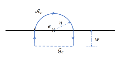
We define the oriented contour 𝒜e{\mathcal{A}}_{e}, depicted in Fig. 3, by

𝒜e={eη+iy:y[w,0]}{e+ηeia:a[π,2π]}{e+η+iy:y[0,w]}.{\mathcal{A}}_{e}=\big\{e-\eta+{\rm i}y:y\in[-w,0]\big\}\cup\big\{e+\eta e^{ia}:a\in[\pi,2\pi]\big\}\cup\big\{e+\eta+{\rm i}y:y\in[0,-w]\big\}. (4.18)
Refer to caption
Figure 3: The contour 𝒜e{\mathcal{A}}_{e}.

The main result of this section is

Proposition 4.2

Suppose that

|λ|+ηaϰ4,λ2ϰ41andλ2α+|λ|ϰ4η1.|\lambda|+\eta\prec\frac{a}{\varkappa_{4}},\quad\lambda^{2}\varkappa_{4}\prec 1\quad\mbox{and}\quad\lambda^{2}\frac{\alpha+|\lambda|\varkappa_{4}}{\eta}\prec 1. (4.19)

Then

Je(t)\displaystyle J_{e}(t) =\displaystyle= s𝒮edeceit(e+λ2ae(s)(e,λ))ϕ,Qe(s)(e,λ)ψ+s𝒮eosceitEe(s)(λ)ϕ,Qe(s)(Ee(s)(λ),λ)ψ\displaystyle\sum_{s\in{\mathcal{S}}_{e}^{\rm dec}}e^{{\rm i}t(e+\lambda^{2}a_{e}^{(s)}(e,\lambda))}\big\langle\phi,Q_{e}^{(s)}(e,\lambda)\psi\big\rangle+\sum_{s\in{\mathcal{S}}_{e}^{\rm osc}}\,e^{{\rm i}tE_{e}^{(s)}(\lambda)}\big\langle\phi,Q_{e}^{(s)}(E_{e}^{(s)}(\lambda),\lambda)\psi\big\rangle (4.20)
12πi𝒜eeitzϕ,(LSz)1PRψdz+Se,\displaystyle-\frac{1}{2\pi{\rm i}}\int_{{\mathcal{A}}_{e}}\,e^{{\rm i}tz}\big\langle\phi,(L_{\rm S}-z)^{-1}P_{\rm R}\psi\big\rangle\,dz+S_{e},

where

Se\displaystyle\|S_{e}\|\prec (4.21)
{ewtw+ηη(ηg+λ2+ϰ3(|λ|+η))+λ2\displaystyle\ \ \ \Big\{e^{wt}\frac{w+\eta}{\eta}\Big(\frac{\eta}{g}+\lambda^{2}+\varkappa_{3}(|\lambda|+\eta)\Big)+\lambda^{2}
+ηewt(ϰ3+λ2ϰ5+(ϰ4κa+ϰ3)(1+ηaλ2))}ϕψ\displaystyle\qquad+\eta e^{wt}\Big(\varkappa_{3}+\lambda^{2}\varkappa_{5}+\Big(\frac{\varkappa_{4}\kappa}{a}+\varkappa_{3}\Big)\Big(1+\frac{\eta}{a\lambda^{2}}\Big)\Big)\Big\}\|\phi\|\,\|\psi\|
+{κηa|λ|ewt+|λ|(1+η(1+ϰ3))+(w+η)ewtη(|λ|+λ2)\displaystyle+\Big\{\frac{\kappa\eta}{a|\lambda|}e^{wt}+|\lambda|\big(1+\eta(1+\varkappa_{3})\big)+\frac{(w+\eta)e^{wt}}{\eta}(|\lambda|+\lambda^{2})
+ewtλ2ηϰ5(|λ|+λ2)+λ2(1+(w+η)ewt(1+ϰ3))}\displaystyle\qquad+e^{wt}\lambda^{2}\eta\varkappa_{5}(|\lambda|+\lambda^{2})+\lambda^{2}\Big(1+(w+\eta)e^{wt}(1+\varkappa_{3})\Big)\Big\}
×[maxjC2(IφjΩ,ϕ)maxjC2(IφjΩ,ψ)+𝔖ϕψϕmaxjC2(IφjΩR,ψ)]\displaystyle\qquad\times\Big[\max_{j}C_{2}(I\varphi_{j}\otimes\Omega,\phi)\max_{j}C_{2}(I\varphi_{j}\otimes\Omega,\psi)+{\mathfrak{S}}_{\phi\leftrightarrow\psi}\|\phi\|\max_{j}C_{2}(I\varphi_{j}\otimes\Omega_{\rm R},\psi)\Big]
+ηewtC2(ϕ,ψ)\displaystyle+\eta e^{wt}C_{2}(\phi,\psi) (4.22)

with the various constants defined in Section 4.2.

Proof of Proposition 4.2. We show (4.20) by estimating separately the three contributions coming from the decomposition (4.3) of the resolvent RzR_{z},

𝒢eeitzRz𝑑z\displaystyle\int_{{\mathcal{G}}_{e}}e^{{\rm i}tz}R_{z}dz =\displaystyle= 𝒢eeitz𝔉(z)1𝑑z+𝒢eeitz𝔅(z)𝑑z+𝒢eeitzRzQ𝑑z\displaystyle\int_{{\mathcal{G}}_{e}}e^{{\rm i}tz}{\mathfrak{F}}(z)^{-1}dz+\int_{{\mathcal{G}}_{e}}e^{{\rm i}tz}{\mathfrak{B}}(z)dz+\int_{{\mathcal{G}}_{e}}e^{{\rm i}tz}R^{Q}_{z}dz (4.23)
\displaystyle\equiv D1+D2+D3.\displaystyle D_{1}+D_{2}+D_{3}.

The corresponding bounds are presented in (4.65), (4.83) and (4.84) below.

Estimate of D1D_{1} in (4.23). Our main estimate for D1D_{1} is given in (4.65) below. All estimates in this section are controlled in the operator norm sense for operators on RanPe{\rm Ran}P_{e}. We have

𝔉(z)=ez+λ2Ae(z,λ),{\mathfrak{F}}(z)=e-z+\lambda^{2}A_{e}(z,\lambda), (4.24)

where the properties of Ae(z,λ)=PeIRzPeIPe,A_{e}(z,\lambda)=-P_{e}IR_{z}^{P_{e}}IP_{e}, are discussed in Section 5.2. It follows from (5.15) that

𝔉(z)1=s=1meQe(s)(z,λ)ez+λ2ae(s)(z,λ).{\mathfrak{F}}(z)^{-1}=\sum_{s=1}^{m_{e}}\frac{Q_{e}^{(s)}(z,\lambda)}{e-z+\lambda^{2}a_{e}^{(s)}(z,\lambda)}. (4.25)

\bullet Consider (4.25) for an s𝒮edecs\in{\mathcal{S}}_{e}^{\rm dec}. The case s𝒮eoscs\in{\mathcal{S}}_{e}^{\rm osc} is dealt with below. Let z𝒢ez\in{\mathcal{G}}_{e}. We show that

Qe(s)(z,λ)ez+λ2ae(s)(z,λ)=Qe(s)(e,λ)ez+λ2ae(s)(e,λ)+T(z,λ),\frac{Q_{e}^{(s)}(z,\lambda)}{e-z+\lambda^{2}a_{e}^{(s)}(z,\lambda)}=\frac{Q_{e}^{(s)}(e,\lambda)}{e-z+\lambda^{2}a_{e}^{(s)}(e,\lambda)}+T(z,\lambda), (4.26)

where (recall the definitions (3.8) and (3.9) of a,αa,\alpha)

T(z,λ)(ϰ4κa+ϰ3)(1+α+|λ|ϰ4a).\|T(z,\lambda)\|\prec\Big(\frac{\varkappa_{4}\kappa}{a}+\varkappa_{3}\Big)\Big(1+\frac{\alpha+|\lambda|\varkappa_{4}}{a}\Big). (4.27)

To show (4.26), we start with the expression for T(z,λ)T(z,\lambda),

T(z,λ)\displaystyle T(z,\lambda) =\displaystyle= T(z,λ)+T′′(z,λ)\displaystyle T^{\prime}(z,\lambda)+T^{\prime\prime}(z,\lambda)
T(z,λ)\displaystyle T^{\prime}(z,\lambda) =\displaystyle= λ2Qe(s)(z,λ)ae(s)(z,λ)ae(s)(e,λ)ezez[ez+λ2ae(s)(z,λ)][ez+λ2ae(s)(e,λ)]\displaystyle-\lambda^{2}Q_{e}^{(s)}(z,\lambda)\frac{a_{e}^{(s)}(z,\lambda)-a_{e}^{(s)}(e,\lambda)}{e-z}\frac{e-z}{[e-z+\lambda^{2}a_{e}^{(s)}(z,\lambda)][e-z+\lambda^{2}a_{e}^{(s)}(e,\lambda)]}
T′′(z,λ)\displaystyle T^{\prime\prime}(z,\lambda) =\displaystyle= Qe(s)(z,λ)Qe(s)(e,λ)ez+λ2ae(s)(e,λ).\displaystyle\frac{Q_{e}^{(s)}(z,\lambda)-Q_{e}^{(s)}(e,\lambda)}{e-z+\lambda^{2}a_{e}^{(s)}(e,\lambda)}. (4.28)

Recall that ae(s)(e,0)=ae(s)a_{e}^{(s)}(e,0)=a_{e}^{(s)} is an eigenvalue of Λe\Lambda_{e}. We have

|ez+λ2ae(s)(z,λ)|\displaystyle|e-z+\lambda^{2}a_{e}^{(s)}(z,\lambda)| (4.29)
=\displaystyle= |ez+λ2ae(s)+λ2(ae(s)(e,λ)ae(s))+λ2(ae(s)(z,λ)ae(s)(e,λ))|\displaystyle\big|e-z+\lambda^{2}a_{e}^{(s)}+\lambda^{2}(a_{e}^{(s)}(e,\lambda)-a_{e}^{(s)})+\lambda^{2}\big(a_{e}^{(s)}(z,\lambda)-a_{e}^{(s)}(e,\lambda)\big)\big|
\displaystyle\geq |ez+λ2ae(s)|Cλ2ϰ4(|λ|+|ze|),\displaystyle|e-z+\lambda^{2}a_{e}^{(s)}|-C\lambda^{2}\varkappa_{4}\big(|\lambda|+|z-e|\big),

where we have used (5.17) (see also Corollary 5.2). Now |ez+λ2ae(s)|Im(ez+λ2ae(s))λ2Imae(s)aλ2|e-z+\lambda^{2}a_{e}^{(s)}|\geq{\rm Im}(e-z+\lambda^{2}a_{e}^{(s)})\geq\lambda^{2}{\rm Im}a_{e}^{(s)}\geq a\lambda^{2} (see (3.8)), so (4.29) yields |ez+λ2ae(s)(z,λ)|aλ2/2|e-z+\lambda^{2}a_{e}^{(s)}(z,\lambda)|\geq a\lambda^{2}/2, since ϰ4(|λ|+|ze|)a\varkappa_{4}\big(|\lambda|+|z-e|\big)\prec a by (4.19) (note that z𝒢ez\in{\mathcal{G}}_{e} so we have |ze|w2+η22η|z-e|\leq\sqrt{w^{2}+\eta^{2}}\leq\sqrt{2}\,\eta (we will take w0w\rightarrow 0 at fixed η\eta, so w<ηw<\eta without loss of generality)). We get

1|ez+λ2ae(s)(z,λ)|1aλ2.\frac{1}{|e-z+\lambda^{2}a_{e}^{(s)}(z,\lambda)|}\prec\frac{1}{a\lambda^{2}}. (4.30)

Moreover, we have

|ezez+λ2ae(s)(e,λ)|\displaystyle\Big|\frac{e-z}{e-z+\lambda^{2}a_{e}^{(s)}(e,\lambda)}\Big| \displaystyle\leq 1+λ2|ae(s)(e,λ)ez+λ2ae(s)(e,λ)|\displaystyle 1+\lambda^{2}\Big|\frac{a_{e}^{(s)}(e,\lambda)}{e-z+\lambda^{2}a_{e}^{(s)}(e,\lambda)}\Big| (4.31)
\displaystyle\prec 1+|ae(s)(e,λ)|a1+α+|λ|ϰ4a\displaystyle 1+\frac{|a_{e}^{(s)}(e,\lambda)|}{a}\prec 1+\frac{\alpha+|\lambda|\varkappa_{4}}{a}

(use (3.9) and (5.17) in the last estimate). Now we estimate T(z,λ)T^{\prime}(z,\lambda) given in (4.28), using the bound Qe(s)(z,λ)κ\|Q_{e}^{(s)}(z,\lambda)\|\prec\kappa (see (5.30)) and (4.30), (4.31) and (5.17),

T(z,λ)ϰ4κa(1+α+|λ|ϰ4a).\|T^{\prime}(z,\lambda)\|\prec\frac{\varkappa_{4}\kappa}{a}\Big(1+\frac{\alpha+|\lambda|\varkappa_{4}}{a}\Big). (4.32)

To deal with T′′(z,λ)T^{\prime\prime}(z,\lambda) in (4.28) we write

T′′(z,λ)=Qe(s)(z,λ)Qe(s)(e,λ)ezezez+λ2ae(s)(e,λ)T^{\prime\prime}(z,\lambda)=\frac{Q_{e}^{(s)}(z,\lambda)-Q_{e}^{(s)}(e,\lambda)}{e-z}\frac{e-z}{e-z+\lambda^{2}a_{e}^{(s)}(e,\lambda)} (4.33)

and use the bounds (5.16) and (4.31) to get

T′′(z,λ)ϰ3(1+α+|λ|ϰ4a).\|T^{\prime\prime}(z,\lambda)\|\prec\varkappa_{3}\Big(1+\frac{\alpha+|\lambda|\varkappa_{4}}{a}\Big). (4.34)

The combination of (4.32) and (4.34) gives (4.27).

\bullet Next we consider a term in (4.25) with s𝒮eoscs\in{\mathcal{S}}_{e}^{\rm osc}. We have to modify the above argument, since it used that the imaginary part of ae(s)a_{e}^{(s)} was strictly positive, which is not the case any more now. By the isospectrality of the Feshbach map, there is exactly one eigenvalue Ee(s)(λ)E_{e}^{(s)}(\lambda) of LλL_{\lambda} with

Ee(s)(λ)=e+λ2ae(s)(Ee(s)(λ),λ).E_{e}^{(s)}(\lambda)=e+\lambda^{2}a_{e}^{(s)}\big(E_{e}^{(s)}(\lambda),\lambda\big). (4.35)

Moreover, the projection Qe(s)(Ee(s)(λ),λ)Q_{e}^{(s)}(E_{e}^{(s)}(\lambda),\lambda) is orthogonal and so it has norm one ([11], Theorem 3.8). We decompose

Qe(s)(z,λ)ez+λ2ae(s)(z,λ)\displaystyle\frac{Q_{e}^{(s)}(z,\lambda)}{e-z+\lambda^{2}a_{e}^{(s)}(z,\lambda)} =\displaystyle= Qe(s)(Ee(s)(λ),λ)Ee(s)(λ)z+Qe(s)(z,λ)Qe(s)(Ee(s)(λ),λ)ez+λ2ae(s)(z,λ)\displaystyle\frac{Q_{e}^{(s)}(E_{e}^{(s)}(\lambda),\lambda)}{E_{e}^{(s)}(\lambda)-z}+\frac{Q_{e}^{(s)}(z,\lambda)-Q_{e}^{(s)}(E_{e}^{(s)}(\lambda),\lambda)}{e-z+\lambda^{2}a_{e}^{(s)}(z,\lambda)} (4.36)
+Qe(s)(Ee(s)(λ),λ)OPENEe(s)(λ)eλ2ae(s)(z,λ))(Ee(s)(λ)z)(ez+λ2ae(s)(z,λ)).\displaystyle+Q_{e}^{(s)}(E_{e}^{(s)}(\lambda),\lambda)\frac{E_{e}^{(s)}(\lambda)-e-\lambda^{2}a_{e}^{(s)}(z,\lambda))}{(E_{e}^{(s)}(\lambda)-z)(e-z+\lambda^{2}a_{e}^{(s)}(z,\lambda))}.

Using (4.35), the second term on the right side of (4.36) becomes

Qe(s)(Ee(s)(λ),λ)Qe(s)(z,λ)Ee(s)(λ)zλ2[ae(s)(Ee(s)(λ),λ)ae(s)(z,λ)]\displaystyle-\frac{Q_{e}^{(s)}(E_{e}^{(s)}(\lambda),\lambda)-Q_{e}^{(s)}(z,\lambda)}{E_{e}^{(s)}(\lambda)-z-\lambda^{2}[a_{e}^{(s)}(E_{e}^{(s)}(\lambda),\lambda)-a_{e}^{(s)}(z,\lambda)]} (4.37)
=Qe(s)(Ee(s)(λ),λ)Qe(s)(z,λ)Ee(s)(λ)z11λ2ae(s)(Ee(s)(λ),λ)ae(s)(z,λ)Ee(s)(λ)z.\displaystyle\qquad=-\frac{Q_{e}^{(s)}(E_{e}^{(s)}(\lambda),\lambda)-Q_{e}^{(s)}(z,\lambda)}{E_{e}^{(s)}(\lambda)-z}\frac{1}{1-\lambda^{2}\,\frac{a_{e}^{(s)}(E_{e}^{(s)}(\lambda),\lambda)-a_{e}^{(s)}(z,\lambda)}{E_{e}^{(s)}(\lambda)-z}}.

We estimate the last fraction in (4.37) by using (5.17) as

|[1λ2ae(s)(Ee(s)(λ),λ)ae(s)(z,λ)Ee(s)(λ)z]1|11Cλ2ϰ41,\Big|\Big[1-\lambda^{2}\,\frac{a_{e}^{(s)}(E_{e}^{(s)}(\lambda),\lambda)-a_{e}^{(s)}(z,\lambda)}{E_{e}^{(s)}(\lambda)-z}\Big]^{-1}\Big|\leq\frac{1}{1-C\lambda^{2}\varkappa_{4}}\prec 1, (4.38)

where the last relations holds since λ2ϰ41\lambda^{2}\varkappa_{4}\prec 1 (see (4.19)). Estimates (4.38) and (5.16) show

(4.37)ϰ3.\Big\|\eqref{m72}\Big\|\prec\varkappa_{3}. (4.39)

Consider now the last term on the right side of (4.36). Using (4.35), the fraction reads

λ2ae(s)(Ee(s)(λ),λ)ae(s)(z,λ)(Ee(s)(λ)z)211λ2ae(s)(Ee(s)(λ),λ)ae(s)(z,λ)Ee(s)(λ)z.\displaystyle\lambda^{2}\ \frac{a_{e}^{(s)}(E_{e}^{(s)}(\lambda),\lambda)-a_{e}^{(s)}(z,\lambda)}{(E_{e}^{(s)}(\lambda)-z)^{2}}\frac{1}{1-\lambda^{2}\,\frac{a_{e}^{(s)}(E_{e}^{(s)}(\lambda),\lambda)-a_{e}^{(s)}(z,\lambda)}{E_{e}^{(s)}(\lambda)-z}}. (4.40)

The second fraction in (4.40) is 1\prec 1 by (4.38). Next, we obtain from point 3. of Lemma 5.1

|ae(s)(Ee(s)(λ),λ)ae(s)(z,λ)Ee(s)(λ)zzae(s)(Ee(s)(λ),λ)|\displaystyle\Big|\frac{a_{e}^{(s)}(E_{e}^{(s)}(\lambda),\lambda)-a_{e}^{(s)}(z,\lambda)}{E_{e}^{(s)}(\lambda)-z}-\partial_{z}a_{e}^{(s)}(E_{e}^{(s)}(\lambda),\lambda)\Big| (4.41)
=\displaystyle= |zEe(s)(λ)(ζae(s)(ζ,λ)ζae(s)(Ee(s)(λ),λ))dζEe(s)(λ)z|\displaystyle\Big|\int_{z}^{E_{e}^{(s)}(\lambda)}\big(\partial_{\zeta}a_{e}^{(s)}(\zeta,\lambda)-\partial_{\zeta}a_{e}^{(s)}(E_{e}^{(s)}(\lambda),\lambda)\big)\frac{d\zeta}{E_{e}^{(s)}(\lambda)-z}\Big|
=\displaystyle= |zEe(s)(λ)dζEe(s)(λ)zζEe(s)(λ)dww2ae(s)(w,λ)|ϰ5|Ee(s)(λ)z|.\displaystyle\Big|\int_{z}^{E_{e}^{(s)}(\lambda)}\frac{d\zeta}{E_{e}^{(s)}(\lambda)-z}\int_{\zeta}^{E_{e}^{(s)}(\lambda)}dw\ \partial_{w}^{2}a_{e}^{(s)}(w,\lambda)\Big|\prec\varkappa_{5}|E_{e}^{(s)}(\lambda)-z|.

It follows that

|ae(s)(Ee(s)(λ),λ)ae(s)(z,λ)(Ee(s)(λ)z)2zae(s)(Ee(s)(λ),λ)Ee(s)(λ)z|ϰ5.\Big|\frac{a_{e}^{(s)}(E_{e}^{(s)}(\lambda),\lambda)-a_{e}^{(s)}(z,\lambda)}{(E_{e}^{(s)}(\lambda)-z)^{2}}-\frac{\partial_{z}a_{e}^{(s)}(E_{e}^{(s)}(\lambda),\lambda)}{E_{e}^{(s)}(\lambda)-z}\Big|\prec\varkappa_{5}. (4.42)

Now

(4.40)=λ2zae(s)(Ee(s)(λ),λ)Ee(s)(λ)z11λ2zae(s)(Ee(s)(λ),λ)+T′′′,\eqref{m75}=\lambda^{2}\frac{\partial_{z}a_{e}^{(s)}(E_{e}^{(s)}(\lambda),\lambda)}{E_{e}^{(s)}(\lambda)-z}\ \frac{1}{1-\lambda^{2}\partial_{z}a_{e}^{(s)}(E_{e}^{(s)}(\lambda),\lambda)}+T^{\prime\prime\prime}, (4.43)

where

T′′′\displaystyle T^{\prime\prime\prime} =\displaystyle= λ2(ae(s)(z,λ)ae(s)(z,λ)(Ee(s)(λ)z)2zae(s)(Ee(s)(λ),λ)Ee(s)(λ)z)11λ2ae(s)(Ee(s)(λ),λ)ae(s)(z,λ)Ee(s)(λ)z\displaystyle\lambda^{2}\Big(\frac{a_{e}^{(s)}(z,\lambda)-a_{e}^{(s)}(z,\lambda)}{(E_{e}^{(s)}(\lambda)-z)^{2}}-\frac{\partial_{z}a_{e}^{(s)}(E_{e}^{(s)}(\lambda),\lambda)}{E_{e}^{(s)}(\lambda)-z}\Big)\frac{1}{1-\lambda^{2}\frac{a_{e}^{(s)}(E_{e}^{(s)}(\lambda),\lambda)-a_{e}^{(s)}(z,\lambda)}{E_{e}^{(s)}(\lambda)-z}} (4.44)
+λ2zae(s)(Ee(s)(λ),λ)Ee(s)(λ)z(11λ2ae(s)(Ee(s)(λ),λ)ae(s)(z,λ)Ee(s)(λ)z11λ2zae(s)(Ee(s)(λ),λ)).\displaystyle+\lambda^{2}\frac{\partial_{z}a_{e}^{(s)}(E_{e}^{(s)}(\lambda),\lambda)}{E_{e}^{(s)}(\lambda)-z}\Big(\frac{1}{1-\lambda^{2}\frac{a_{e}^{(s)}(E_{e}^{(s)}(\lambda),\lambda)-a_{e}^{(s)}(z,\lambda)}{E_{e}^{(s)}(\lambda)-z}}-\frac{1}{1-\lambda^{2}\partial_{z}a_{e}^{(s)}(E_{e}^{(s)}(\lambda),\lambda)}\Big).

By (5.17), |zae(s)(Ee(s)(λ),λ)|ϰ4|\partial_{z}a_{e}^{(s)}(E_{e}^{(s)}(\lambda),\lambda)|\prec\varkappa_{4} and so the second fraction in (4.43) is bounded 1\prec 1 since λ2ϰ41\lambda^{2}\varkappa_{4}\prec 1 (see (4.19)).

The estimates (4.42) and (4.38) show that the first summand on the right side of (4.44) is λ2ϰ5\prec\lambda^{2}\varkappa_{5}. Next,

1Ee(s)(λ)z([1λ2ae(s)(Ee(s)(λ),λ)ae(s)(z,λ)Ee(s)(λ)z]1[1λ2zae(s)(Ee(s)(λ),λ)]1)\displaystyle\frac{1}{E_{e}^{(s)}(\lambda)-z}\Big(\Big[1-\lambda^{2}\frac{a_{e}^{(s)}(E_{e}^{(s)}(\lambda),\lambda)-a_{e}^{(s)}(z,\lambda)}{E_{e}^{(s)}(\lambda)-z}\Big]^{-1}-\Big[1-\lambda^{2}\partial_{z}a_{e}^{(s)}(E_{e}^{(s)}(\lambda),\lambda)\Big]^{-1}\Big) (4.45)
=\displaystyle= λ2zae(s)(Ee(s)(λ),λ)ae(s)(Ee(s)(λ),λ)ae(s)(z,λ)Ee(s)(λ)zEe(s)(λ)z\displaystyle\lambda^{2}\frac{\partial_{z}a_{e}^{(s)}(E_{e}^{(s)}(\lambda),\lambda)-\frac{a_{e}^{(s)}(E_{e}^{(s)}(\lambda),\lambda)-a_{e}^{(s)}(z,\lambda)}{E_{e}^{(s)}(\lambda)-z}}{E_{e}^{(s)}(\lambda)-z}
×[1λ2ae(s)(Ee(s)(λ),λ)ae(s)(z,λ)Ee(s)(λ)z]1[1λ2zae(s)(Ee(s)(λ),λ)]1\displaystyle\times\big[1-\lambda^{2}\frac{a_{e}^{(s)}(E_{e}^{(s)}(\lambda),\lambda)-a_{e}^{(s)}(z,\lambda)}{E_{e}^{(s)}(\lambda)-z}\big]^{-1}\big[1-\lambda^{2}\partial_{z}a_{e}^{(s)}(E_{e}^{(s)}(\lambda),\lambda)\big]^{-1}

which has modulus λ2ϰ5\prec\lambda^{2}\varkappa_{5} (use (4.38), (4.42), (5.17)). In conclusion, we obtain

|T′′′|λ2ϰ5.|T^{\prime\prime\prime}|\prec\lambda^{2}\varkappa_{5}. (4.46)

Combining (4.36), (4.39), (4.43) and (4.46), and also using that Qe(s)(Ee(s)(λ),λ)=1\|Q_{e}^{(s)}(E_{e}^{(s)}(\lambda),\lambda)\|=1 (c.f. after (4.35)), gives the bound for s𝒮eoscs\in{\mathcal{S}}_{e}^{\rm osc},

\displaystyle\Big\| Qe(s)(z,λ)ez+λ2ae(s)(z,λ)Qe(s)(Ee(s)(λ),λ)Ee(s)(λ)z[1+λ2zae(s)(Ee(s)(λ),λ)1λ2zae(s)(Ee(s)(λ),λ)]\displaystyle\frac{Q_{e}^{(s)}(z,\lambda)}{e-z+\lambda^{2}a_{e}^{(s)}(z,\lambda)}-\frac{Q_{e}^{(s)}(E_{e}^{(s)}(\lambda),\lambda)}{E_{e}^{(s)}(\lambda)-z}\Big[1+\lambda^{2}\frac{\partial_{z}a_{e}^{(s)}(E_{e}^{(s)}(\lambda),\lambda)}{1-\lambda^{2}\partial_{z}a_{e}^{(s)}(E_{e}^{(s)}(\lambda),\lambda)}\Big]\Big\|
ϰ3+λ2ϰ5.\displaystyle\prec\varkappa_{3}+\lambda^{2}\varkappa_{5}. (4.47)

\bullet Combining (4.25), (4.26) and (4.47) shows that for every e0e\in{\mathcal{E}}_{0},

𝔉(z)1\displaystyle{\mathfrak{F}}(z)^{-1} =\displaystyle= s𝒮edecQe(s)(e,λ)ez+λ2ae(s)(e,λ)\displaystyle\sum_{s\in{\mathcal{S}}_{e}^{\rm dec}}\frac{Q_{e}^{(s)}(e,\lambda)}{e-z+\lambda^{2}a_{e}^{(s)}(e,\lambda)} (4.48)
+s𝒮eoscQe(s)(Ee(s)(λ),λ)Ee(s)(λ)z[1+λ2zae(s)(Ee(s)(λ),λ)1λ2zae(s)(Ee(s)(λ),λ)]+𝒯(z,λ),\displaystyle+\sum_{s\in{\mathcal{S}}_{e}^{\rm osc}}\frac{Q_{e}^{(s)}(E_{e}^{(s)}(\lambda),\lambda)}{E_{e}^{(s)}(\lambda)-z}\Big[1+\lambda^{2}\ \frac{\partial_{z}a_{e}^{(s)}(E_{e}^{(s)}(\lambda),\lambda)}{1-\lambda^{2}\partial_{z}a_{e}^{(s)}(E_{e}^{(s)}(\lambda),\lambda)}\Big]+{\mathcal{T}}(z,\lambda),

where the remainder satisfies

𝒯(z,λ)ϰ3+λ2ϰ5+(ϰ4κa+ϰ3)(1+α+|λ|ϰ4a).\|{\mathcal{T}}(z,\lambda)\|\prec\varkappa_{3}+\lambda^{2}\varkappa_{5}+\Big(\frac{\varkappa_{4}\kappa}{a}+\varkappa_{3}\Big)\Big(1+\frac{\alpha+|\lambda|\varkappa_{4}}{a}\Big). (4.49)

We now analyze D1D_{1}, see (4.23). From (4.48),

D1𝒢eeitz𝔉(z)1𝑑z=Qe(s)(e,λ)s𝒮edec𝒢eeitzez+λ2ae(s)(e,λ)𝑑z\displaystyle D_{1}\equiv\int_{{\mathcal{G}}_{e}}e^{{\rm i}tz}\,{\mathfrak{F}}(z)^{-1}dz=Q_{e}^{(s)}(e,\lambda)\sum_{s\in{\mathcal{S}}_{e}^{\rm dec}}\int_{{\mathcal{G}}_{e}}\,\frac{e^{{\rm i}tz}}{e-z+\lambda^{2}a_{e}^{(s)}(e,\lambda)}\,dz\ (4.50)
+\displaystyle+ s𝒮eoscQe(s)(Ee(s)(λ),λ)[1+λ2zae(s)(Ee(s)(λ),λ)1λ2zae(s)(Ee(s)(λ),λ)]𝒢eeitzEe(s)(λ)z𝑑z+S1,\displaystyle\sum_{s\in{\mathcal{S}}_{e}^{\rm osc}}Q_{e}^{(s)}(E_{e}^{(s)}(\lambda),\lambda)\Big[1+\lambda^{2}\frac{\partial_{z}a_{e}^{(s)}(E_{e}^{(s)}(\lambda),\lambda)}{1-\lambda^{2}\partial_{z}a_{e}^{(s)}(E_{e}^{(s)}(\lambda),\lambda)}\Big]\int_{{\mathcal{G}}_{e}}\frac{e^{{\rm i}tz}}{E_{e}^{(s)}(\lambda)-z}dz+S_{1},

where the remainder S1S_{1} is due to the integration of 𝒯(z,λ){\mathcal{T}}(z,\lambda), estimated by (take into account that |𝒢e|=2η|{\mathcal{G}}_{e}|=2\eta)

S1\displaystyle\|S_{1}\| \displaystyle\prec ηewt(ϰ3+λ2ϰ5+(ϰ4κa+ϰ3)(1+α+|λ|ϰ4a))\displaystyle\eta e^{wt}\Big(\varkappa_{3}+\lambda^{2}\varkappa_{5}+\Big(\frac{\varkappa_{4}\kappa}{a}+\varkappa_{3}\Big)\Big(1+\frac{\alpha+|\lambda|\varkappa_{4}}{a}\Big)\Big)
\displaystyle\prec ηewt(ϰ3+λ2ϰ5+(ϰ4κa+ϰ3)(1+ηaλ2)).\displaystyle\eta e^{wt}\Big(\varkappa_{3}+\lambda^{2}\varkappa_{5}+\Big(\frac{\varkappa_{4}\kappa}{a}+\varkappa_{3}\Big)\Big(1+\frac{\eta}{a\lambda^{2}}\Big)\Big).

We used (4.19) in the second estimate. Now

𝒢eeitzEe(s)(λ)z𝑑z=2πieitEe(s)(λ)+𝒜eeitzEe(s)(λ)z𝑑z,\int_{{\mathcal{G}}_{e}}\frac{e^{{\rm i}tz}}{E_{e}^{(s)}(\lambda)-z}dz=-2\pi{\rm i}e^{{\rm i}tE_{e}^{(s)}(\lambda)}+\int_{{\mathcal{A}}_{e}}\frac{e^{{\rm i}tz}}{E_{e}^{(s)}(\lambda)-z}dz, (4.51)

where 𝒜e{\mathcal{A}}_{e} is given in (4.18). Note that by (4.35) and (5.17), |Ee(s)(λ)e|=λ2|ae(s)(Ee(s)(λ),λ)|λ2|ae(s)|+λ2ϰ4(|Ee(s)(λ)e|+|λ|)|E_{e}^{(s)}(\lambda)-e|=\lambda^{2}|a_{e}^{(s)}(E_{e}^{(s)}(\lambda),\lambda)|\prec\lambda^{2}|a_{e}^{(s)}|+\lambda^{2}\varkappa_{4}(|E_{e}^{(s)}(\lambda)-e|+|\lambda|), which, since λ2ϰ41\lambda^{2}\varkappa_{4}\prec 1 (see (4.19)), we can solve for (see (3.9)):

|Ee(s)(λ)e|λ2(α+|λ|ϰ4)η.\displaystyle|E_{e}^{(s)}(\lambda)-e|\prec\lambda^{2}(\alpha+|\lambda|\varkappa_{4})\prec\eta. (4.52)

In the last estimate, we used that

λ2α+|λ|ϰ4η1\lambda^{2}\frac{\alpha+|\lambda|\varkappa_{4}}{\eta}\prec 1 (4.53)

(see (4.19)). Thus (4.51) gives

|𝒢eeitzEe(s)(λ)z𝑑z|1+(w+η)ewtη.\Big|\int_{{\mathcal{G}}_{e}}\frac{e^{{\rm i}tz}}{E_{e}^{(s)}(\lambda)-z}dz\Big|\prec 1+\frac{(w+\eta)e^{wt}}{\eta}. (4.54)

Using this bound in (4.50) shows that

D1\displaystyle\Big\|D_{1} \displaystyle- s𝒮edec𝒢eeitzQe(s)(e,λ)ez+λ2ae(s)(e,λ)dzs𝒮eosc𝒢eeitzQe(s)(Ee(s)(λ),λ)Ee(s)(λ)zdz\displaystyle\sum_{s\in{\mathcal{S}}_{e}^{\rm dec}}\int_{{\mathcal{G}}_{e}}\,\frac{e^{{\rm i}tz}Q_{e}^{(s)}(e,\lambda)}{e-z+\lambda^{2}a_{e}^{(s)}(e,\lambda)}\,dz-\sum_{s\in{\mathcal{S}}_{e}^{\rm osc}}\int_{{\mathcal{G}}_{e}}\,\frac{e^{{\rm i}tz}Q_{e}^{(s)}(E_{e}^{(s)}(\lambda),\lambda)}{E_{e}^{(s)}(\lambda)-z}\,dz\ \Big\| (4.55)
\displaystyle\prec S1+λ2(1+(w+η)ewtη).\displaystyle\|S_{1}\|+\lambda^{2}\Big(1+\frac{(w+\eta)e^{wt}}{\eta}\Big).

Similarly to (4.51), we also write the contour integrals in the first sum in (4.55) as

𝒢eeitzez+λ2ae(s)(e,λ)𝑑z=2πieit(e+λ2ae(s)(e,λ))+𝒜eeitzez+λ2ae(s)(e,λ)𝑑z,\int_{{\mathcal{G}}_{e}}\frac{e^{{\rm i}tz}}{e-z+\lambda^{2}a_{e}^{(s)}(e,\lambda)}dz=-2\pi{\rm i}e^{{\rm i}t(e+\lambda^{2}a_{e}^{(s)}(e,\lambda))}+\int_{{\mathcal{A}}_{e}}\frac{e^{{\rm i}tz}}{e-z+\lambda^{2}a_{e}^{(s)}(e,\lambda)}dz, (4.56)

where 𝒜e{\mathcal{A}}_{e} is the contour (4.18). For z𝒜ez\in{\mathcal{A}}_{e} we have |ze|η|z-e|\geq\eta and so λ2|ae(s)(e,λ)/(ez)|<1\lambda^{2}|a_{e}^{(s)}(e,\lambda)/(e-z)|<1 (because we have λ2(α+|λ|ϰ4)/η<1\lambda^{2}(\alpha+|\lambda|\varkappa_{4})/\eta<1). Thus the geometric series converges,

1ez+λ2ae(s)(e,λ)=1ezn0(λ2ae(s)(e,λ)ez)n,\displaystyle\frac{1}{e-z+\lambda^{2}a_{e}^{(s)}(e,\lambda)}=\frac{1}{e-z}\sum_{n\geq 0}\big(-\frac{\lambda^{2}a_{e}^{(s)}(e,\lambda)}{e-z}\big)^{n}, (4.57)

and gives the bound

|1ez+λ2ae(s)(e,λ)1ez|λ2η(α+|λ|ϰ4).\Big|\frac{1}{e-z+\lambda^{2}a_{e}^{(s)}(e,\lambda)}-\frac{1}{e-z}\Big|\prec\frac{\lambda^{2}}{\eta}(\alpha+|\lambda|\varkappa_{4}). (4.58)

With |𝒜e|=2w+πη|{\mathcal{A}}_{e}|=2w+\pi\eta, we obtain

|𝒜eeitzez+λ2ae(s)(e,λ)𝑑z𝒜eeitzez𝑑z|ewtw+ηηλ2(α+|λ|ϰ4).\Big|\int_{{\mathcal{A}}_{e}}\frac{e^{{\rm i}tz}}{e-z+\lambda^{2}a_{e}^{(s)}(e,\lambda)}dz-\int_{{\mathcal{A}}_{e}}\frac{e^{{\rm i}tz}}{e-z}dz\Big|\prec e^{wt}\frac{w+\eta}{\eta}\lambda^{2}(\alpha+|\lambda|\varkappa_{4}). (4.59)

In the same way we obtain

|𝒜eeitzEe(s)(λ)z𝑑z𝒜eeitzez𝑑z|ewtw+ηηλ2(α+|λ|ϰ4).\Big|\int_{{\mathcal{A}}_{e}}\frac{e^{{\rm i}tz}}{E_{e}^{(s)}(\lambda)-z}dz-\int_{{\mathcal{A}}_{e}}\frac{e^{{\rm i}tz}}{e-z}dz\Big|\prec e^{wt}\frac{w+\eta}{\eta}\lambda^{2}(\alpha+|\lambda|\varkappa_{4}). (4.60)

Then using (4.56) and (4.59) in (4.55) (and similarly for the integrals over the singularity (Ee(s)(λ)z)1(E_{e}^{(s)}(\lambda)-z)^{-1}) gives

D1\displaystyle\Big\|D_{1} +\displaystyle+ s𝒮edec[2πieit(e+λ2ae(s)(e,λ))Qe(s)(e,λ)𝒜eeitzQe(s)(e,λ)ez𝑑z]\displaystyle\sum_{s\in{\mathcal{S}}_{e}^{\rm dec}}\Big[2\pi{\rm i}\,e^{{\rm i}t(e+\lambda^{2}a_{e}^{(s)}(e,\lambda))}Q_{e}^{(s)}(e,\lambda)-\int_{{\mathcal{A}}_{e}}\frac{e^{{\rm i}tz}Q_{e}^{(s)}(e,\lambda)}{e-z}dz\Big] (4.61)
+s𝒮eosc[2πieitEe(s)(λ)Qe(s)(Ee(s)(λ),λ)𝒜eeitzQe(s)(Ee(s)(λ),λ)ezdz]\displaystyle+\sum_{s\in{\mathcal{S}}_{e}^{\rm osc}}\Big[2\pi{\rm i}\,e^{{\rm i}tE_{e}^{(s)}(\lambda)}Q_{e}^{(s)}(E_{e}^{(s)}(\lambda),\lambda)-\int_{{\mathcal{A}}_{e}}\frac{e^{{\rm i}tz}Q_{e}^{(s)}(E_{e}^{(s)}(\lambda),\lambda)}{e-z}dz\Big]\Big\|
\displaystyle\prec S1+λ2(1+(w+η)ewtη(1+κ(α+|λ|ϰ4))).\displaystyle\|S_{1}\|+\lambda^{2}\Big(1+\frac{(w+\eta)e^{wt}}{\eta}\big(1+\kappa(\alpha+|\lambda|\varkappa_{4})\big)\Big).

Next we replace the projections in the remaining integrals in (4.61) by their values at λ=0\lambda=0: By (5.16) we have Qe(s)(e,λ)Qe(s)(e,0)|λ|ϰ3\|Q_{e}^{(s)}(e,\lambda)-Q_{e}^{(s)}(e,0)\|\prec|\lambda|\varkappa_{3} and Qe(s)(Ee(s)(λ),λ)Qe(s)(e,0)ϰ3(|Ee(s)(λ)e|+|λ|)|λ|ϰ3[1+|λ|(α+|λ|ϰ4)]ϰ3(|λ|+η)\|Q_{e}^{(s)}(E_{e}^{(s)}(\lambda),\lambda)-Q_{e}^{(s)}(e,0)\|\prec\varkappa_{3}(|E_{e}^{(s)}(\lambda)-e|+|\lambda|)\prec|\lambda|\varkappa_{3}[1+|\lambda|(\alpha+|\lambda|\varkappa_{4})]\prec\varkappa_{3}(|\lambda|+\eta), see also (4.52), (4.19). Upon replacing the projections in the integrals of (4.61) by their values at λ=0\lambda=0, we thus make an error (w+η)ewtηϰ3(|λ|+η)\prec\frac{(w+\eta)e^{wt}}{\eta}\varkappa_{3}(|\lambda|+\eta). Once this replacement is made, we use the fact that s=1meQe(s)(e,0)=Pe\sum_{s=1}^{m_{e}}Q_{e}^{(s)}(e,0)=P_{e} is the spectral projection of L0L_{0} associated to the eigenvalue ee and so we get from (4.61)

D1\displaystyle D_{1} =\displaystyle= 2πis𝒮edeceit(e+λ2ae(s)(e,λ))Qe(s)(e,λ)2πis𝒮eosceitEe(s)(λ)Qe(s)(Ee(s)(λ),λ)\displaystyle-2\pi{\rm i}\sum_{s\in{\mathcal{S}}_{e}^{\rm dec}}\,e^{{\rm i}t(e+\lambda^{2}a_{e}^{(s)}(e,\lambda))}Q_{e}^{(s)}(e,\lambda)-2\pi{\rm i}\sum_{s\in{\mathcal{S}}_{e}^{\rm osc}}\,e^{{\rm i}tE_{e}^{(s)}(\lambda)}Q_{e}^{(s)}(E_{e}^{(s)}(\lambda),\lambda) (4.62)
+𝒜eeitzPeezdz+S2,\displaystyle+\int_{{\mathcal{A}}_{e}}\frac{e^{{\rm i}tz}P_{e}}{e-z}dz+S_{2},

where

S2S1+λ2+ewt(w+η)η(λ2(1+κ(α+|λ|ϰ4))+ϰ3(|λ|+η)).\|S_{2}\|\prec\|S_{1}\|+\lambda^{2}+\frac{e^{wt}(w+\eta)}{\eta}\Big(\lambda^{2}\big(1+\kappa(\alpha+|\lambda|\varkappa_{4})\big)+\varkappa_{3}(|\lambda|+\eta)\Big). (4.63)

We now further analyze the integral in (4.62). Denoting PS,e=1lSPS,eP^{\perp}_{{\rm S},e}=\mathchoice{\rm 1\mskip-4.0mul}{\rm 1\mskip-4.0mul}{\rm 1\mskip-4.5mul}{\rm 1\mskip-5.0mul}_{\rm S}-P_{{\rm S},e}, where PS,eP_{{\rm S},e} is the spectral projection of LSL_{\rm S} onto the eigenspace associated to ee (see (2.10)), we have (as η<g/2\eta<g/2)

𝒜eeitzLSz𝑑zPS,eewt(w+η)g,\Big\|\int_{{\mathcal{A}}_{e}}\frac{e^{{\rm i}tz}}{L_{\rm S}-z}dz\,P^{\perp}_{{\rm S},e}\Big\|\prec\frac{e^{wt}(w+\eta)}{g}, (4.64)

where gg is the spectral gap of LSL_{\rm S}, (2.17). So we can replace Pe=PS,ePRP_{e}=P_{{\rm S},e}\otimes P_{\rm R} in (4.62) by simply PRP_{\rm R}, incurring an error of size of the right hand side of (4.64),

D1\displaystyle D_{1} =\displaystyle= 2πis𝒮edeceit(e+λ2ae(s)(e,λ))Qe(s)(e,λ)2πis𝒮eosceitEe(s)(λ)Qe(s)(Ee(s)(λ),λ)\displaystyle-2\pi{\rm i}\sum_{s\in{\mathcal{S}}_{e}^{\rm dec}}\,e^{{\rm i}t(e+\lambda^{2}a_{e}^{(s)}(e,\lambda))}Q_{e}^{(s)}(e,\lambda)-2\pi{\rm i}\sum_{s\in{\mathcal{S}}_{e}^{\rm osc}}\,e^{{\rm i}tE_{e}^{(s)}(\lambda)}Q_{e}^{(s)}(E_{e}^{(s)}(\lambda),\lambda) (4.65)
+𝒜eeitzPRLSzdz+S3,\displaystyle+\int_{{\mathcal{A}}_{e}}\,\frac{e^{{\rm i}tz}P_{\rm R}}{L_{\rm S}-z}\,dz+S_{3},

with

S3S1+λ2+ewt(w+η)η(ηg+λ2(1+κ(α+|λ|ϰ4))+ϰ3(|λ|+η)).\|S_{3}\|\prec\|S_{1}\|+\lambda^{2}+\frac{e^{wt}(w+\eta)}{\eta}\Big(\frac{\eta}{g}+\lambda^{2}\big(1+\kappa(\alpha+|\lambda|\varkappa_{4})\big)+\varkappa_{3}(|\lambda|+\eta)\Big). (4.66)

Estimate of D2D_{2} in (4.23). Our main estimate is given in (4.83) below. We have from (4.5) with Q=PeQ=P_{e},

ϕ,D2ψ=𝒢eeitzϕ,(z)ψ𝑑z\displaystyle\langle\phi,D_{2}\psi\rangle=\int_{{\mathcal{G}}_{e}}e^{{\rm i}tz}\langle\phi,{\mathcal{B}}(z)\psi\rangle dz (4.67)
=\displaystyle= 𝒢eeitzϕ,{λ𝔉(z)1PeIRzPeλRzPeIPe𝔉(z)1+λ2RzPeIPe𝔉(z)1PeIRzPe}ψ𝑑z.\displaystyle\int_{{\mathcal{G}}_{e}}e^{{\rm i}tz}\langle\phi,\,\{-\lambda\,{\mathfrak{F}}(z)^{-1}P_{e}IR_{z}^{P_{e}}-\lambda R_{z}^{P_{e}}IP_{e}{\mathfrak{F}}(z)^{-1}+\lambda^{2}R_{z}^{P_{e}}IP_{e}{\mathfrak{F}}(z)^{-1}P_{e}IR_{z}^{P_{e}}\}\,\psi\rangle\,dz.

We begin by analyzing the first term on the right side of (4.67). Using (5.15),

𝒢eeitzϕ,𝔉(z)1λPeIRzPeψ𝑑z=λs=1me𝒢eeitzϕ,Qe(s)(z,λ)PeIRzPeψez+λ2ae(s)(z,λ)𝑑z.\int_{{\mathcal{G}}_{e}}e^{{\rm i}tz}\langle\phi,\,{\mathfrak{F}}(z)^{-1}\lambda P_{e}IR_{z}^{P_{e}}\psi\rangle dz=\lambda\sum_{s=1}^{m_{e}}\int_{{\mathcal{G}}_{e}}e^{{\rm i}tz}\frac{\langle\phi,Q_{e}^{(s)}(z,\lambda)P_{e}IR^{P_{e}}_{z}\psi\rangle}{e-z+\lambda^{2}a_{e}^{(s)}(z,\lambda)}dz. (4.68)

\bullet For s𝒮edecs\in{\mathcal{S}}_{e}^{\rm dec} we have from (4.30)

|λs=1me𝒢eeitzϕ,Qe(s)(z,λ)PeIRzPeψez+λ2ae(s)(z,λ)𝑑z|\displaystyle\Big|\lambda\sum_{s=1}^{m_{e}}\int_{{\mathcal{G}}_{e}}e^{{\rm i}tz}\frac{\langle\phi,Q_{e}^{(s)}(z,\lambda)P_{e}IR^{P_{e}}_{z}\psi\rangle}{e-z+\lambda^{2}a_{e}^{(s)}(z,\lambda)}dz\Big| \displaystyle\prec |𝒢e|a|λ|ewtmaxz𝒢e|ϕ,Qe(s)(z,λ)PeIRzPeψ|\displaystyle\frac{|{\mathcal{G}}_{e}|}{a|\lambda|}e^{wt}\max_{z\in{\mathcal{G}}_{e}}|\langle\phi,Q_{e}^{(s)}(z,\lambda)P_{e}IR^{P_{e}}_{z}\psi\rangle| (4.69)
\displaystyle\prec κηa|λ|ewtϕmaxjC2(IφjΩ,ψ).\displaystyle\frac{\kappa\eta}{a|\lambda|}e^{wt}\|\phi\|\max_{j}C_{2}(I\varphi_{j}\otimes\Omega,\psi).\quad

To get the last bound, we took into account that Pe=PePΩP_{e}=P_{e}P_{\Omega}, that IPe𝒟IP_{e}\subset{\mathcal{D}}, so that from (5.30) and (4.8), we obtain

|ϕ,Qe(s)(z,λ)PeIRzPeψ|\displaystyle|\langle\phi,Q_{e}^{(s)}(z,\lambda)P_{e}IR^{P_{e}}_{z}\psi\rangle| \displaystyle\leq j|ϕ,Qe(s)(z,λ)φjΩ||φjΩ,IRzPeψ|\displaystyle\sum_{j}|\langle\phi,Q_{e}^{(s)}(z,\lambda)\varphi_{j}\otimes\Omega\rangle|\ |\langle\varphi_{j}\otimes\Omega,IR_{z}^{P_{e}}\psi\rangle| (4.70)
\displaystyle\prec κϕmaxjC2(IφjΩ,ψ).\displaystyle\kappa\|\phi\|\max_{j}C_{2}(I\varphi_{j}\otimes\Omega,\psi).

\bullet For s𝒮eoscs\in{\mathcal{S}}_{e}^{\rm osc} we use (4.35) to get

Qe(s)(z,λ)PeIRzPeez+λ2ae(s)(z,λ)=Qe(s)(z,λ)PeIRzPeEe(s)(λ)z11λ2ae(s)(Ee(s)(λ),λ)ae(s)(z,λ)Ee(s)(λ)z.\frac{Q_{e}^{(s)}(z,\lambda)P_{e}IR_{z}^{P_{e}}}{e-z+\lambda^{2}a_{e}^{(s)}(z,\lambda)}=\frac{Q_{e}^{(s)}(z,\lambda)P_{e}IR_{z}^{P_{e}}}{E_{e}^{(s)}(\lambda)-z}\frac{1}{1-\lambda^{2}\frac{a_{e}^{(s)}(E_{e}^{(s)}(\lambda),\lambda)-a_{e}^{(s)}(z,\lambda)}{E_{e}^{(s)}(\lambda)-z}}. (4.71)

Now

Qe(s)(z,λ)PeIRzPeEe(s)(λ)z=Qe(s)(z,λ)Qe(s)(Ee(s)(λ),λ)Ee(s)(λ)zPeIRzPe\displaystyle\frac{Q_{e}^{(s)}(z,\lambda)P_{e}IR_{z}^{P_{e}}}{E_{e}^{(s)}(\lambda)-z}=\frac{Q_{e}^{(s)}(z,\lambda)-Q_{e}^{(s)}(E_{e}^{(s)}(\lambda),\lambda)}{E_{e}^{(s)}(\lambda)-z}P_{e}IR_{z}^{P_{e}} (4.72)
Qe(s)(Ee(s)(λ),λ)PeIREe(s)(λ)PeRzPeEe(s)(λ)z+Qe(s)(Ee(s)(λ),λ)PeIREe(s)(λ)PeEe(s)(λ)z.\displaystyle-Q_{e}^{(s)}(E_{e}^{(s)}(\lambda),\lambda)P_{e}I\frac{R^{P_{e}}_{E_{e}^{(s)}(\lambda)}-R_{z}^{P_{e}}}{E_{e}^{(s)}(\lambda)-z}+\frac{Q_{e}^{(s)}(E_{e}^{(s)}(\lambda),\lambda)P_{e}IR_{E_{e}^{(s)}(\lambda)}^{P_{e}}}{E_{e}^{(s)}(\lambda)-z}.

The first two terms of the right side of (4.72), when used in (4.71), are estimated by taking into account that the second factor on the right side of (4.71) is 1\prec 1 due to (4.38). However, the last term on the right side of (4.72) has a singularity in zz which must be removed by integrating over 𝒢e{\mathcal{G}}_{e}. To do this, we write

11λ2ae(s)(Ee(s)(λ),λ)ae(s)(z,λ)Ee(s)(λ)z=11λ2zae(s)(Ee(s)(λ),λ)\displaystyle\frac{1}{1-\lambda^{2}\frac{a_{e}^{(s)}(E_{e}^{(s)}(\lambda),\lambda)-a_{e}^{(s)}(z,\lambda)}{E_{e}^{(s)}(\lambda)-z}}=\frac{1}{1-\lambda^{2}\partial_{z}a_{e}^{(s)}(E_{e}^{(s)}(\lambda),\lambda)}
λ2zae(s)(Ee(s)(λ),λ)ae(s)(Ee(s)(λ),λ)ae(s)(z,λ)Ee(s)(λ)z[1λ2zae(s)(Ee(s)(λ),λ)][1λ2ae(s)(Ee(s)(λ),λ)ae(s)(z,λ)Ee(s)(λ)z].\displaystyle-\lambda^{2}\frac{\partial_{z}a_{e}^{(s)}(E_{e}^{(s)}(\lambda),\lambda)-\frac{a_{e}^{(s)}(E_{e}^{(s)}(\lambda),\lambda)-a_{e}^{(s)}(z,\lambda)}{E_{e}^{(s)}(\lambda)-z}}{[1-\lambda^{2}\partial_{z}a_{e}^{(s)}(E_{e}^{(s)}(\lambda),\lambda)][1-\lambda^{2}\frac{a_{e}^{(s)}(E_{e}^{(s)}(\lambda),\lambda)-a_{e}^{(s)}(z,\lambda)}{E_{e}^{(s)}(\lambda)-z}]}.

The denominator of the second summand on the right side is 1\succ 1 and its numerator is ϰ5|Ee(s)(λ)z|\prec\varkappa_{5}|E_{e}^{(s)}(\lambda)-z| by (4.41). Thus

|𝒢eeitzEe(s)(λ)z11λ2ae(s)(Ee(s)(λ),λ)ae(s)(z,λ)Ee(s)(λ)zdz\displaystyle\Big|\int_{{\mathcal{G}}_{e}}\frac{e^{{\rm i}tz}}{E_{e}^{(s)}(\lambda)-z}\frac{1}{1-\lambda^{2}\frac{a_{e}^{(s)}(E_{e}^{(s)}(\lambda),\lambda)-a_{e}^{(s)}(z,\lambda)}{E_{e}^{(s)}(\lambda)-z}}dz (4.73)
11λ2zae(s)(Ee(s)(λ),λ)𝒢eeitzEe(s)(λ)zdz|ewtλ2|𝒢e|ϰ5ewtλ2ηϰ5.\displaystyle-\frac{1}{1-\lambda^{2}\partial_{z}a_{e}^{(s)}(E_{e}^{(s)}(\lambda),\lambda)}\int_{{\mathcal{G}}_{e}}\frac{e^{{\rm i}tz}}{E_{e}^{(s)}(\lambda)-z}dz\Big|\prec e^{wt}\lambda^{2}|{\mathcal{G}}_{e}|\varkappa_{5}\prec e^{wt}\lambda^{2}\eta\varkappa_{5}.\qquad

Now |1λ2zae(s)(Ee(s)(λ),λ)|11|1-\lambda^{2}\partial_{z}a_{e}^{(s)}(E_{e}^{(s)}(\lambda),\lambda)|^{-1}\prec 1 (see (4.19)) and so by (4.73) and (4.54), we have

|𝒢eeitzEe(s)(λ)z11λ2ae(s)(Ee(s)(λ),λ)ae(s)(z,λ)Ee(s)(λ)z𝑑z|1+(w+η)ewtη+ewtλ2ηϰ5.\Big|\int_{{\mathcal{G}}_{e}}\frac{e^{{\rm i}tz}}{E_{e}^{(s)}(\lambda)-z}\frac{1}{1-\lambda^{2}\frac{a_{e}^{(s)}(E_{e}^{(s)}(\lambda),\lambda)-a_{e}^{(s)}(z,\lambda)}{E_{e}^{(s)}(\lambda)-z}}dz\Big|\prec 1+\frac{(w+\eta)e^{wt}}{\eta}+e^{wt}\lambda^{2}\eta\varkappa_{5}. (4.74)

We combine (4.74) with (4.71), (4.72) to get

|λ𝒢eeitzϕ,Qe(s)(z,λ)PeIRzPeψez+λ2ae(s)(z,λ)𝑑z|\displaystyle\Big|\lambda\int_{{\mathcal{G}}_{e}}e^{{\rm i}tz}\frac{\langle\phi,Q_{e}^{(s)}(z,\lambda)P_{e}IR^{P_{e}}_{z}\psi\rangle}{e-z+\lambda^{2}a_{e}^{(s)}(z,\lambda)}dz\Big| (4.75)
\displaystyle\prec |λ||ϕ,Qe(s)(Ee(s)(λ),λ)PeIREe(s)(λ)Peψ|(1+(w+η)ewtη+ewtλ2ηϰ5)\displaystyle|\lambda||\langle\phi,Q_{e}^{(s)}(E_{e}^{(s)}(\lambda),\lambda)P_{e}IR_{E_{e}^{(s)}(\lambda)}^{P_{e}}\psi\rangle|\Big(1+\frac{(w+\eta)e^{wt}}{\eta}+e^{wt}\lambda^{2}\eta\varkappa_{5}\Big)
+|λ||𝒢e|maxz𝒢e|ϕ,Qe(s)(z,λ)Qe(s)(Ee(s)(λ),λ)Ee(s)(λ)zPeIRzPeψ|\displaystyle+|\lambda||{\mathcal{G}}_{e}|\max_{z\in{\mathcal{G}}_{e}}\Big|\langle\phi,\frac{Q_{e}^{(s)}(z,\lambda)-Q_{e}^{(s)}(E_{e}^{(s)}(\lambda),\lambda)}{E_{e}^{(s)}(\lambda)-z}P_{e}IR_{z}^{P_{e}}\psi\rangle\Big|
+|λ||𝒢e|maxz𝒢e|ϕ,Qe(s)(Ee(s)(λ),λ)PeIREe(s)(λ)PeRzPeEe(s)(λ)zψ|.\displaystyle+|\lambda||{\mathcal{G}}_{e}|\max_{z\in{\mathcal{G}}_{e}}\Big|\langle\phi,Q_{e}^{(s)}(E_{e}^{(s)}(\lambda),\lambda)P_{e}I\frac{R^{P_{e}}_{E_{e}^{(s)}(\lambda)}-R_{z}^{P_{e}}}{E_{e}^{(s)}(\lambda)-z}\psi\rangle\Big|.

Using (4.54) and the argument of (4.70) (with Qe(s)(Ee(s)(λ),λ)=1\|Q_{e}^{(s)}(E_{e}^{(s)}(\lambda),\lambda)\|=1 as this one is an orthogonal projection) we get |ϕ,Qe(s)(Ee(s)(λ),λ)PeIREe(s)(λ)Peψ|ϕmaxjC2(IφjΩ,ψ)|\langle\phi,Q_{e}^{(s)}(E_{e}^{(s)}(\lambda),\lambda)P_{e}IR_{E_{e}^{(s)}(\lambda)}^{P_{e}}\psi\rangle|\prec\|\phi\|\max_{j}C_{2}(I\varphi_{j}\otimes\Omega,\psi). Next, by (5.16), (4.8) and again by the argument of (4.70), the last two terms on the right hand side of (4.75) has an upper bound |λ|ηϕ(1+ϰ3)maxjC2(IφjΩ,ψ)\prec|\lambda|\eta\|\phi\|(1+\varkappa_{3})\max_{j}C_{2}(I\varphi_{j}\otimes\Omega,\psi). We thus obtain from (4.75) that for s𝒮eoscs\in{\mathcal{S}}_{e}^{\rm osc},

|λ𝒢eeitzϕ,Qe(s)(z,λ)PeIRzPeψez+λ2ae(s)(z,λ)𝑑z|\displaystyle\Big|\lambda\int_{{\mathcal{G}}_{e}}e^{{\rm i}tz}\frac{\langle\phi,Q_{e}^{(s)}(z,\lambda)P_{e}IR^{P_{e}}_{z}\psi\rangle}{e-z+\lambda^{2}a_{e}^{(s)}(z,\lambda)}dz\Big| (4.76)
\displaystyle\prec |λ|ϕmaxjC2(IφjΩ,ψ)(1+(w+η)ewtη+ewtλ2ηϰ5+η(1+ϰ3)).\displaystyle|\lambda|\|\phi\|\max_{j}C_{2}(I\varphi_{j}\otimes\Omega,\psi)\Big(1+\frac{(w+\eta)e^{wt}}{\eta}+e^{wt}\lambda^{2}\eta\varkappa_{5}+\eta(1+\varkappa_{3})\Big).

\bullet The relations (4.68), (4.69) and (4.76) give

|𝒢eeitzϕ,𝔉(z)1λPeIRzPeψ𝑑z|ϕmaxjC2(IφjΩ,ψ)\displaystyle\Big|\int_{{\mathcal{G}}_{e}}e^{{\rm i}tz}\langle\phi,\,{\mathfrak{F}}(z)^{-1}\lambda P_{e}IR_{z}^{P_{e}}\psi\rangle dz\Big|\prec\|\phi\|\max_{j}C_{2}(I\varphi_{j}\otimes\Omega,\psi) (4.77)
×(κηa|λ|ewt+|λ|(1+(w+η)ewtη+ewtλ2ηϰ5+η(1+ϰ3))).\displaystyle\times\Big(\frac{\kappa\eta}{a|\lambda|}e^{wt}+|\lambda|\big(1+\frac{(w+\eta)e^{wt}}{\eta}+e^{wt}\lambda^{2}\eta\varkappa_{5}+\eta(1+\varkappa_{3})\big)\Big).\qquad

The integral 𝒢eeitzϕ,λRzPeIPe𝔉(z)1ψ𝑑z\int_{{\mathcal{G}}_{e}}e^{{\rm i}tz}\langle\phi,\lambda R_{z}^{P_{e}}IP_{e}{\mathfrak{F}}(z)^{-1}\psi\rangle dz in (4.67) has the same upper bound (4.77), but with ϕ\phi and ψ\psi interchanged.

\bullet We now estimate the term in (4.67) involving λ2RzPeI𝔉(z)1IRzPe\lambda^{2}R_{z}^{P_{e}}I{\mathfrak{F}}(z)^{-1}IR_{z}^{P_{e}}. We use again (4.25). Proceeding as above, we obtain from (4.30) that for s𝒮edecs\in{\mathcal{S}}_{e}^{\rm dec},

λ2|𝒢eeitzϕ,RzPeIPeQe(s)(z,λ)IRzPeψez+λ2ae(s)(z,λ)𝑑z|ηewtamaxz𝒢e|ϕ,RzPeIPeQe(s)(z,λ)IRzPeψ|.\lambda^{2}\Big|\int_{{\mathcal{G}}_{e}}e^{{\rm i}tz}\frac{\langle\phi,R^{P_{e}}_{z}IP_{e}Q_{e}^{(s)}(z,\lambda)IR_{z}^{P_{e}}\,\psi\rangle}{e-z+\lambda^{2}a_{e}^{(s)}(z,\lambda)}\,dz\Big|\prec\frac{\eta e^{wt}}{a}\max_{z\in{\mathcal{G}}_{e}}|\langle\phi,R_{z}^{P_{e}}IP_{e}Q_{e}^{(s)}(z,\lambda)IR_{z}^{P_{e}}\psi\rangle|. (4.78)

Now

|ϕ,RzPeIPeQe(s)(z,λ)IRzPeψ|Qe(s)(z,λ)PeI(RzPe)ϕPeIRzPeψ|\langle\phi,R_{z}^{P_{e}}IP_{e}Q_{e}^{(s)}(z,\lambda)IR_{z}^{P_{e}}\psi\rangle|\prec\|Q_{e}^{(s)}(z,\lambda)\|\|P_{e}I(R_{z}^{P_{e}})^{*}\phi\|\|P_{e}IR_{z}^{P_{e}}\psi\| (4.79)

and

PeI(RzPe)ϕ\displaystyle\|P_{e}I(R_{z}^{P_{e}})^{*}\phi\| \displaystyle\prec maxj|φjΩ,I(RzPe)ϕ|=maxj|ϕ,RzPeIφjΩ|\displaystyle\max_{j}|\langle\varphi_{j}\otimes\Omega,I(R_{z}^{P_{e}})^{*}\phi\rangle|=\max_{j}|\langle\phi,R_{z}^{P_{e}}I\varphi_{j}\otimes\Omega\rangle|
\displaystyle\prec maxjC2(ϕ,IφjΩ)\displaystyle\max_{j}C_{2}(\phi,I\varphi_{j}\otimes\Omega)

and similarly, PeIRzPeψmaxjC2(IφjΩ,ψ)\|P_{e}IR_{z}^{P_{e}}\psi\|\prec\max_{j}C_{2}(I\varphi_{j}\otimes\Omega,\psi). Furthermore by (5.30), Qe(s)(z,λ)κ\|Q_{e}^{(s)}(z,\lambda)\|\prec\kappa. Combining these estimates with (4.78) yields that for all s𝒮edecs\in{\mathcal{S}}_{e}^{\rm dec},

λ2|𝒢eeitz\displaystyle\lambda^{2}\Big|\int_{{\mathcal{G}}_{e}}e^{{\rm i}tz} ϕ,RzPeIPeQe(s)(z,λ)IRzPeψez+λ2ae(s)(z,λ)dz|\displaystyle\frac{\langle\phi,R^{P_{e}}_{z}IP_{e}Q_{e}^{(s)}(z,\lambda)IR_{z}^{P_{e}}\,\psi\rangle}{e-z+\lambda^{2}a_{e}^{(s)}(z,\lambda)}\,dz\Big|
ηewtaκmaxjC2(IφjΩ,ϕ)maxjC2(IφjΩ,ψ).\displaystyle\prec\frac{\eta e^{wt}}{a}\kappa\max_{j}C_{2}(I\varphi_{j}\otimes\Omega,\phi)\max_{j}C_{2}(I\varphi_{j}\otimes\Omega,\psi). (4.80)

Next we treat the case s𝒮eoscs\in{\mathcal{S}}_{e}^{\rm osc}, for which we show the bound (recall that e=Ee(s)(λ)+λ2ae(s)(Ee(s)(λ),λ)e=E_{e}^{(s)}(\lambda)+\lambda^{2}a_{e}^{(s)}(E_{e}^{(s)}(\lambda),\lambda), (4.35))

λ2|𝒢eeitz\displaystyle\lambda^{2}\Big|\int_{{\mathcal{G}}_{e}}e^{{\rm i}tz} ϕ,RzPeIPeQe(s)(z,λ)IRzPeψEe(s)(λ)zλ2[ae(s)(Ee(s)(λ),λ)ae(s)(z,λ)]dz|\displaystyle\frac{\langle\phi,R^{P_{e}}_{z}IP_{e}Q_{e}^{(s)}(z,\lambda)IR_{z}^{P_{e}}\,\psi\rangle}{E_{e}^{(s)}(\lambda)-z-\lambda^{2}[a_{e}^{(s)}(E_{e}^{(s)}(\lambda),\lambda)-a_{e}^{(s)}(z,\lambda)]}\,dz\Big|
λ2(1+(w+η)ewt(1+1η+ϰ3)+ewtλ2ηϰ5)\displaystyle\prec\lambda^{2}\Big(1+(w+\eta)e^{wt}(1+\tfrac{1}{\eta}+\varkappa_{3})+e^{wt}\lambda^{2}\eta\varkappa_{5}\Big)
×maxjC2(IφjΩ,ϕ)maxjC2(IφjΩ,ψ)\displaystyle\quad\times\max_{j}C_{2}(I\varphi_{j}\otimes\Omega,\phi)\max_{j}C_{2}(I\varphi_{j}\otimes\Omega,\psi)\qquad (4.81)

as follows. We proceed as in (4.71) and (4.72) and get terms with [Qe(s)(Ee(s)(λ),λ)Qe(s)(z,λ)][Ee(s)(λ)z]1[Q_{e}^{(s)}(E_{e}^{(s)}(\lambda),\lambda)-Q_{e}^{(s)}(z,\lambda)][E_{e}^{(s)}(\lambda)-z]^{-1} and [REe(s)(λ)PeRzPe][Ee(s)(λ)z]1[R_{E_{e}^{(s)}(\lambda)}^{P_{e}}-R_{z}^{P_{e}}][E_{e}^{(s)}(\lambda)-z]^{-1}, all of which are controlled by bounds on the derivatives. We find that they are λ2(η+w)ewt(1+ϰ3)maxjC2(IφjΩ,ϕ)maxjC2(IφjΩ,ψ)\prec\lambda^{2}(\eta+w)e^{wt}(1+\varkappa_{3})\max_{j}C_{2}(I\varphi_{j}\otimes\Omega,\phi)\max_{j}C_{2}(I\varphi_{j}\otimes\Omega,\psi). The only remaining term to consider is

λ2|ϕ,\displaystyle\lambda^{2}|\langle\phi, REe(s)(λ)PeIPeQe(s)(Ee(s)(λ),λ)IREe(s)(λ)Peψ|\displaystyle R^{P_{e}}_{E_{e}^{(s)}(\lambda)}IP_{e}Q_{e}^{(s)}(E_{e}^{(s)}(\lambda),\lambda)IR_{E_{e}^{(s)}(\lambda)}^{P_{e}}\,\psi\rangle|
×\displaystyle\times |𝒢eeitzEe(s)(λ)z11λ2ae(s)(Ee(s)(λ),λ)ae(s)(z,λ)Ee(s)(λ)z𝑑z|\displaystyle\Big|\int_{{\mathcal{G}}_{e}}\frac{e^{{\rm i}tz}}{E_{e}^{(s)}(\lambda)-z}\frac{1}{1-\lambda^{2}\frac{a_{e}^{(s)}(E_{e}^{(s)}(\lambda),\lambda)-a_{e}^{(s)}(z,\lambda)}{E_{e}^{(s)}(\lambda)-z}}dz\Big|
λ2(1+(w+η)ewtη+ewtλ2ηϰ5)maxjC2(IφjΩ,ϕ)maxjC2(IφjΩ,ψ),\displaystyle\prec\lambda^{2}\Big(1+\frac{(w+\eta)e^{wt}}{\eta}+e^{wt}\lambda^{2}\eta\varkappa_{5}\Big)\max_{j}C_{2}(I\varphi_{j}\otimes\Omega,\phi)\max_{j}C_{2}(I\varphi_{j}\otimes\Omega,\psi), (4.82)

where we have used (4.74). This yields (4.81).

We collect the estimates (4.77), (4.81) and use them in (4.67) to get

|ϕ,D2\displaystyle|\langle\phi,D_{2} ψ|{κηa|λ|ewt+|λ|(1+η(1+ϰ3))+(w+η)ewtη(|λ|+λ2)\displaystyle\psi\rangle|\prec\Big\{\frac{\kappa\eta}{a|\lambda|}e^{wt}+|\lambda|\big(1+\eta(1+\varkappa_{3})\big)+\frac{(w+\eta)e^{wt}}{\eta}(|\lambda|+\lambda^{2})
+ewtλ2ηϰ5(|λ|+λ2)+λ2(1+(w+η)ewt(1+ϰ3))}\displaystyle+e^{wt}\lambda^{2}\eta\varkappa_{5}(|\lambda|+\lambda^{2})+\lambda^{2}\Big(1+(w+\eta)e^{wt}(1+\varkappa_{3})\Big)\Big\}
×[maxjC2(IφjΩ,ϕ)maxjC2(IφjΩ,ψ)+𝔖ϕψϕmaxjC2(IφjΩR,ψ)].\displaystyle\times\Big[\max_{j}C_{2}(I\varphi_{j}\otimes\Omega,\phi)\max_{j}C_{2}(I\varphi_{j}\otimes\Omega,\psi)+{\mathfrak{S}}_{\phi\leftrightarrow\psi}\|\phi\|\max_{j}C_{2}(I\varphi_{j}\otimes\Omega_{\rm R},\psi)\Big]. (4.83)

Estimate of D3D_{3} in (4.23). The bound (4.8) gives immediately

|ϕ,D3ψ|=|𝒢eeitzϕ,RzPeψ𝑑z|ηewtC2(ϕ,ψ).\big|\langle\phi,D_{3}\psi\rangle\big|=\Big|\int_{{\mathcal{G}}_{e}}e^{{\rm i}tz}\langle\phi,R_{z}^{P_{e}}\psi\rangle dz\Big|\prec\eta e^{wt}C_{2}(\phi,\psi). (4.84)

The three bounds (4.65), (4.83) and (4.84), together with (4.23), show (4.20) and (4.22) and this completes the proof of Proposition 4.2. \Box

4.4 Analysis of J(t)J_{\infty}(t)

Refer to caption
Figure 4: Different regions for the real part of zz, for z𝒢ez\in{\mathcal{G}}_{\infty}^{e}.

We introduce a new parameter ϑ>0\vartheta>0 which will be chosen suitably small (a power of |λ||\lambda|) below, and which is depicted in Fig. 4. The goal of this section is to show the following result.

Proposition 4.3

If ϰ1λ2/η1\varkappa_{1}\lambda^{2}/\eta\prec 1, then we have

|J(t)\displaystyle\Big|J_{\infty}(t) +12πi𝒢eitzϕ,(LSz)1ψdzϕ,PReitPRLλPRPRψ|\displaystyle+\frac{1}{2\pi{\rm i}}\int_{{\mathcal{G}}_{\infty}}e^{{\rm i}tz}\langle\phi,(L_{\rm S}-z)^{-1}\psi\rangle dz-\langle\phi,P^{\perp}_{\rm R}e^{{\rm i}tP^{\perp}_{\rm R}L_{\lambda}P^{\perp}_{\rm R}}P^{\perp}_{\rm R}\psi\rangle\Big|
\displaystyle\prec λ2ewt[ϰ1η+gϰ1(η+ϑ)2+gϰ12λ2η3\displaystyle\ \lambda^{2}e^{wt}\Big[\frac{\varkappa_{1}}{\eta}+\frac{g\varkappa_{1}}{(\eta+\vartheta)^{2}}+\frac{g\varkappa^{2}_{1}\lambda^{2}}{\eta^{3}}
+ϑ(ϰ1(η+ϑ+|λ|)+ακη2+ϰ1g(1/η+1/g))]ϕψ\displaystyle\qquad\quad+\vartheta\Big(\frac{\varkappa_{1}(\eta+\vartheta+|\lambda|)+\alpha\kappa}{\eta^{2}}+\frac{\varkappa_{1}}{g}\big(1/\eta+1/g\big)\Big)\Big]\|\phi\|\,\|\psi\|
+ηewtC1(ϕ,ψ)\displaystyle+\eta e^{wt}C_{1}(\phi,\psi)
+ewt(|λ|ϑη+|λ|η+ϑ+|λ|3ϰ1η2[1+λ2ϰ1η])𝔖ϕψϕmaxjC1(IφjΩR,ψ)\displaystyle+e^{wt}\Big(\frac{|\lambda|\vartheta}{\eta}+\frac{|\lambda|}{\eta+\vartheta}+\frac{|\lambda|^{3}\varkappa_{1}}{\eta^{2}}\Big[1+\frac{\lambda^{2}\varkappa_{1}}{\eta}\Big]\Big){\mathfrak{S}}_{\phi\leftrightarrow\psi}\|\phi\|\max_{j}C_{1}(I\varphi_{j}\otimes\Omega_{\rm R},\psi)
+ewtλ2η[1+λ2ϰ1(1+1/η)]maxjC1(IφjΩR,ϕ)maxjC1(IφjΩR,ψ)\displaystyle+e^{wt}\frac{\lambda^{2}}{\eta}\Big[1+\lambda^{2}\varkappa_{1}(1+1/\eta)\Big]\max_{j}C_{1}(I\varphi_{j}\otimes\Omega_{\rm R},\phi)\max_{j}C_{1}(I\varphi_{j}\otimes\Omega_{\rm R},\psi)
+ewt|λ|η+ϑ𝔖ϕψϕ(PRIPRψ+maxjC1(IφjΩR,(L¯λ+i)ψ))\displaystyle+e^{wt}\frac{|\lambda|}{\eta+\vartheta}{\mathfrak{S}}_{\phi\leftrightarrow\psi}\|\phi\|\Big(\|P_{\rm R}I\|\|P^{\perp}_{\rm R}\psi\|+\max_{j}C_{1}\big(I\varphi_{j}\otimes\Omega_{\rm R},(\bar{L}_{\lambda}+{\rm i})\psi\big)\Big)
+ewtλ2η𝔖ϕψmaxjC1(IφjΩR,ϕ)(PRIPRψ+maxjC1(IφjΩR,(L¯λ+i)ψ)).\displaystyle+e^{wt}\frac{\lambda^{2}}{\eta}{\mathfrak{S}}_{\phi\leftrightarrow\psi}\max_{j}C_{1}(I\varphi_{j}\otimes\Omega_{\rm R},\phi)\Big(\|P_{\rm R}I\|\|P^{\perp}_{\rm R}\psi\|+\max_{j}C_{1}\big(I\varphi_{j}\otimes\Omega_{\rm R},(\bar{L}_{\lambda}+{\rm i})\psi\big)\Big). (4.85)

In the last line, we use the notation L¯λPRLλPRRanPR\bar{L}_{\lambda}\equiv P^{\perp}_{\rm R}L_{\lambda}P^{\perp}_{\rm R}\upharpoonright_{{\rm Ran}P^{\perp}_{\rm R}}.

Proof of Proposition 4.3. Consider two adjacent eigenvalues e<ee<e^{\prime} of LSL_{\rm S} and set

𝒢e={xiw:e+ηxeη}.{\mathcal{G}}^{e}_{\infty}=\{x-{\rm i}w:e+\eta\leq x\leq e^{\prime}-\eta\}. (4.86)

We introduce a new small parameter ϑ>0\vartheta>0 and set 𝒟1={xiw:e+ηxe+η+ϑ}{\mathcal{D}}_{1}=\{x-{\rm i}w:e+\eta\leq x\leq e+\eta+\vartheta\} and 𝒟2={xiw:e+η+ϑxe+ee2}{\mathcal{D}}_{2}=\{x-{\rm i}w:e+\eta+\vartheta\leq x\leq e+\tfrac{e^{\prime}-e}{2}\}, as depicted in Fig. 4.

We use the Feshbach decomposition (4.3) with Q=PR=|ΩRΩR|Q=P_{\rm R}=|\Omega_{\rm R}\rangle\langle\Omega_{\rm R}| and accordingly, we get three contributions to the resolvent as in (4.23),

𝒢eeitzRz𝑑z\displaystyle\int_{{\mathcal{G}}_{\infty}^{e}}e^{{\rm i}tz}R_{z}dz =\displaystyle= 𝒢eeitz𝔉(z)1𝑑z+𝒢eeitz𝔅(z)𝑑z+𝒢eeitzRzPR𝑑z\displaystyle\int_{{\mathcal{G}}_{\infty}^{e}}e^{{\rm i}tz}{\mathfrak{F}}(z)^{-1}dz+\int_{{\mathcal{G}}_{\infty}^{e}}e^{{\rm i}tz}{\mathfrak{B}}(z)dz+\int_{{\mathcal{G}}_{\infty}^{e}}e^{{\rm i}tz}R^{P_{\rm R}}_{z}dz (4.87)
\displaystyle\equiv D1+D2+D3.\displaystyle D^{\prime}_{1}+D^{\prime}_{2}+D^{\prime}_{3}.

Estimating D1D^{\prime}_{1} of (4.87). The main bound we prove is given in (4.95). We have, in the sense of operators acting on RanPR{\rm Ran}P_{\rm R},

𝔉(z)=PR(LSzλ2IRzPRI)PR=(1lλ2PRIRzPRIPR(LSz)1)(LSz).{\mathfrak{F}}(z)=P_{\rm R}\big(L_{\rm S}-z-\lambda^{2}IR_{z}^{P_{\rm R}}I\big)P_{\rm R}=\big(\mathchoice{\rm 1\mskip-4.0mul}{\rm 1\mskip-4.0mul}{\rm 1\mskip-4.5mul}{\rm 1\mskip-5.0mul}-\lambda^{2}P_{\rm R}IR_{z}^{P_{\rm R}}IP_{\rm R}(L_{\rm S}-z)^{-1}\big)(L_{\rm S}-z). (4.88)

For z𝒢ez\in{\mathcal{G}}_{\infty}^{e}, (LSz)11/η\|(L_{\rm S}-z)^{-1}\|\leq 1/\eta and by (5.2) we get λ2PRIRzPRIPR(LSz)1ϰ1λ2η\|\lambda^{2}P_{\rm R}IR_{z}^{P_{\rm R}}IP_{\rm R}(L_{\rm S}-z)^{-1}\|\prec\frac{\varkappa_{1}\lambda^{2}}{\eta} and so we get from (4.88), since ϰ1λ2η1\frac{\varkappa_{1}\lambda^{2}}{\eta}\prec 1,

𝔉(z)1=(LSz)1[1l+λ2PRIRzPRIPR(LSz)1+S4],S4ϰ12λ4η2.{\mathfrak{F}}(z)^{-1}=(L_{\rm S}-z)^{-1}\big[\mathchoice{\rm 1\mskip-4.0mul}{\rm 1\mskip-4.0mul}{\rm 1\mskip-4.5mul}{\rm 1\mskip-5.0mul}+\lambda^{2}P_{\rm R}IR_{z}^{P_{\rm R}}IP_{\rm R}(L_{\rm S}-z)^{-1}+S_{4}\big],\qquad\|S_{4}\|\prec\frac{\varkappa^{2}_{1}\lambda^{4}}{\eta^{2}}. (4.89)

We consider now z𝒟1𝒟2z\in{\mathcal{D}}_{1}\cup{\mathcal{D}}_{2} (the region closer to ee than to ee^{\prime}, see Fig. 4). By inserting 1lS=PS,e+PS,e\mathchoice{\rm 1\mskip-4.0mul}{\rm 1\mskip-4.0mul}{\rm 1\mskip-4.5mul}{\rm 1\mskip-5.0mul}_{\rm S}=P_{{\rm S},e}+P_{{\rm S},e}^{\perp}, using that Pe=PS,ePRP_{e}=P_{{\rm S},e}\otimes P_{\rm R} and that PS,e(LSz)12/g\|P_{{\rm S},e}^{\perp}(L_{\rm S}-z)^{-1}\|\leq 2/g (see (2.17) for the gap gg), we estimate the term in (4.89) involving the resolvent RzPRR_{z}^{P_{\rm R}} as follows,

λ2(LSz)1PRIRzPRIPR(LSz)1λ2(ez)2PeIRzPRIPeϰ1λ2g(1/η+1/g).\Big\|\lambda^{2}(L_{\rm S}-z)^{-1}P_{\rm R}IR_{z}^{P_{\rm R}}IP_{\rm R}(L_{\rm S}-z)^{-1}-\frac{\lambda^{2}}{(e-z)^{2}}P_{e}IR_{z}^{P_{\rm R}}IP_{e}\Big\|\prec\frac{\varkappa_{1}\lambda^{2}}{g}\big(1/\eta+1/g\big). (4.90)

By (5.2) we have PeIRzPRIPePeI(RePR|λ=0)IPeϰ1(|ze|+|λ|)\|P_{e}IR_{z}^{P_{\rm R}}IP_{e}-P_{e}I(R_{e}^{P_{\rm R}}|_{\lambda=0})IP_{e}\|\prec\varkappa_{1}(|z-e|+|\lambda|). Thus, taking into account the definition (2.12) of the level shift operator Λe\Lambda_{e} and using that PRIPe=PeIPeP^{\perp}_{\rm R}IP_{e}=P^{\perp}_{e}IP_{e}, we have

PeIRzPRIPeΛeϰ1(|ze|+|λ|).\|P_{e}IR_{z}^{P_{\rm R}}IP_{e}-\Lambda_{e}\|\prec\varkappa_{1}\big(|z-e|+|\lambda|\big). (4.91)

The reason for introducing the new small parameter ϑ\vartheta (see Fig. 4), is that for z𝒟1z\in{\mathcal{D}}_{1}, the right hand side of (4.91) is bounded above by ϰ1(η+ϑ+|λ|)\varkappa_{1}(\eta+\vartheta+|\lambda|). It then follows from (4.91) and (4.90) that z𝒟1\forall z\in{\mathcal{D}}_{1},

λ2(LSz)1PRIRzPRIPR(LSz)1λ2Λeη2+ϰ1λ2[η+ϑ+|λ|η2+1g(1/η+1/g)]\|\lambda^{2}(L_{\rm S}-z)^{-1}P_{\rm R}IR_{z}^{P_{\rm R}}IP_{\rm R}(L_{\rm S}-z)^{-1}\|\prec\frac{\lambda^{2}\|\Lambda_{e}\|}{\eta^{2}}+\varkappa_{1}\lambda^{2}\Big[\frac{\eta+\vartheta+|\lambda|}{\eta^{2}}+\frac{1}{g}\big(1/\eta+1/g\big)\Big]

and hence, as Λeακ\|\Lambda_{e}\|\prec\alpha\kappa, we get

𝒟1eitzλ2(LSz)1PRIRzPRIPR(LSz)1𝑑z\displaystyle\Big\|\int_{{\mathcal{D}}_{1}}e^{{\rm i}tz}\lambda^{2}(L_{\rm S}-z)^{-1}P_{\rm R}IR_{z}^{P_{\rm R}}IP_{\rm R}(L_{\rm S}-z)^{-1}dz\Big\| (4.92)
\displaystyle\prec λ2ϑewt[ϰ1(η+ϑ+|λ|)+ακη2+ϰ1g(1/η+1/g)].\displaystyle\lambda^{2}\vartheta e^{wt}\Big[\frac{\varkappa_{1}(\eta+\vartheta+|\lambda|)+\alpha\kappa}{\eta^{2}}+\frac{\varkappa_{1}}{g}\big(1/\eta+1/g\big)\Big].

Next we find a bound for the integral on the left side of (4.92) with 𝒟1{\mathcal{D}}_{1} replaced by 𝒟2{\mathcal{D}}_{2}. For z𝒟2z\in{\mathcal{D}}_{2}, we have (LSz)1(η+ϑ)1\|(L_{\rm S}-z)^{-1}\|\leq(\eta+\vartheta)^{-1} and so it follows from (5.2) that (LSz)1PRIRzPRIPR(LSz)1ϰ1(η+ϑ)2\|(L_{\rm S}-z)^{-1}P_{\rm R}IR_{z}^{P_{\rm R}}IP_{\rm R}(L_{\rm S}-z)^{-1}\|\prec\varkappa_{1}(\eta+\vartheta)^{-2}. Consequently, since |𝒟2|<g/2|{\mathcal{D}}_{2}|<g/2, we get

𝒟2eitzλ2(LSz)1PRIRzPRIPR(LSz)1𝑑zλ2ϰ1gewt(η+ϑ)2.\Big\|\int_{{\mathcal{D}}_{2}}e^{{\rm i}tz}\lambda^{2}(L_{\rm S}-z)^{-1}P_{\rm R}IR_{z}^{P_{\rm R}}IP_{\rm R}(L_{\rm S}-z)^{-1}dz\Big\|\prec\frac{\lambda^{2}\varkappa_{1}ge^{wt}}{(\eta+\vartheta)^{2}}. (4.93)

We now combine (4.92) and (4.93) with (4.89),

𝒟1𝒟1eitz𝔉(z)1𝑑z𝒟1𝒟2eitzLSz𝑑z\displaystyle\Big\|\int_{{\mathcal{D}}_{1}\cup{\mathcal{D}}_{1}}e^{{\rm i}tz}\,{\mathfrak{F}}(z)^{-1}dz-\int_{{\mathcal{D}}_{1}\cup{\mathcal{D}}_{2}}\frac{e^{{\rm i}tz}}{L_{\rm S}-z}dz\Big\| (4.94)
\displaystyle\prec λ2ewt[gϰ1(η+ϑ)2+gϰ12λ2η3+ϑ(ϰ1(η+ϑ+|λ|)+ακη2+ϰ1g(1/η+1/g))].\displaystyle\lambda^{2}e^{wt}\Big[\frac{g\varkappa_{1}}{(\eta+\vartheta)^{2}}+\frac{g\varkappa^{2}_{1}\lambda^{2}}{\eta^{3}}+\vartheta\Big(\frac{\varkappa_{1}(\eta+\vartheta+|\lambda|)+\alpha\kappa}{\eta^{2}}+\frac{\varkappa_{1}}{g}\big(1/\eta+1/g\big)\Big)\Big].

For z𝒢ez\in{\mathcal{G}}_{\infty}^{e} lying closer to ee^{\prime} than ee (i.e., z𝒢e\(𝒟1𝒟2)z\in{\mathcal{G}}_{\infty}^{e}\backslash({\mathcal{D}}_{1}\cup{\mathcal{D}}_{2})) the analysis is the same, as only the distance from xx to the nearest eigenvalue of LSL_{\rm S} plays a role in the estimates. We conclude that the bound (4.94) holds with 𝒟1𝒟2{\mathcal{D}}_{1}\cup{\mathcal{D}}_{2} replaced by 𝒢e{\mathcal{G}}_{\infty}^{e} in the integrals on the left side:

D1𝒢eeitzLSz𝑑z\displaystyle\Big\|D^{\prime}_{1}-\int_{{\mathcal{G}}_{\infty}^{e}}\frac{e^{{\rm i}tz}}{L_{\rm S}-z}dz\Big\| (4.95)
\displaystyle\prec λ2ewt[gϰ1(η+ϑ)2+gϰ12λ2η3+ϑ(ϰ1(η+ϑ+|λ|)+ακη2+ϰ1g(1/η+1/g))].\displaystyle\lambda^{2}e^{wt}\Big[\frac{g\varkappa_{1}}{(\eta+\vartheta)^{2}}+\frac{g\varkappa^{2}_{1}\lambda^{2}}{\eta^{3}}+\vartheta\Big(\frac{\varkappa_{1}(\eta+\vartheta+|\lambda|)+\alpha\kappa}{\eta^{2}}+\frac{\varkappa_{1}}{g}\big(1/\eta+1/g\big)\Big)\Big].

Estimating D2D^{\prime}_{2} of (4.87). Our main etimate is given in (4.102). According to (4.5), the term (z){\mathcal{B}}(z) gives three contributions. The ones involving only one resolvent RzPRR_{z}^{P_{\rm R}} are all estimated in the same way as follows. We have for all zz\in{\mathbb{C}}_{-} (use (2.6)),

|ϕ,𝔉(z)1PRIRzPRψ|maxj|ϕ,𝔉(z)1φjΩR|C1(IφjΩR,ψ).\big|\langle\phi,{\mathfrak{F}}(z)^{-1}P_{\rm R}IR_{z}^{P_{\rm R}}\psi\rangle\big|\prec\max_{j}\big|\langle\phi,{\mathfrak{F}}(z)^{-1}\varphi_{j}\otimes\Omega_{\rm R}\rangle\big|\,C_{1}(I\varphi_{j}\otimes\Omega_{\rm R},\psi). (4.96)

According to (4.89), the main term of 𝔉(z)1{\mathfrak{F}}(z)^{-1} is (LSz)1(L_{\rm S}-z)^{-1} the norm of which is bounded above by 1/η1/\eta for z𝒟1z\in{\mathcal{D}}_{1} and by 1/(η+ϑ)1/(\eta+\vartheta) for z𝒟2z\in{\mathcal{D}}_{2}. Then,

|𝒟1𝒟2eitzϕ,(LSz)1λIRzPRψ𝑑z|ewt(|λ|ϑη+|λ|η+ϑ)ϕmaxjC1(IφjΩR,ψ).\Big|\int_{{\mathcal{D}}_{1}\cup{\mathcal{D}}_{2}}e^{{\rm i}tz}\langle\phi,(L_{\rm S}-z)^{-1}\lambda IR_{z}^{P_{\rm R}}\psi\rangle dz\Big|\prec e^{wt}\Big(\frac{|\lambda|\vartheta}{\eta}+\frac{|\lambda|}{\eta+\vartheta}\Big)\|\phi\|\max_{j}C_{1}(I\varphi_{j}\otimes\Omega_{\rm R},\psi). (4.97)

The terms in (4.89), which are of order two and higher in λ\lambda, are estimated as

(LSz)1[λ2PRIRzPRIPR(LSz)1+S4]λ2ϰ1η2[1+λ2ϰ1η]\Big\|(L_{\rm S}-z)^{-1}\big[\lambda^{2}P_{\rm R}IR_{z}^{P_{\rm R}}IP_{\rm R}(L_{\rm S}-z)^{-1}+S_{4}\big]\Big\|\prec\frac{\lambda^{2}\varkappa_{1}}{\eta^{2}}\Big[1+\frac{\lambda^{2}\varkappa_{1}}{\eta}\Big] (4.98)

for z𝒢ez\in{\mathcal{G}}_{\infty}^{e}. It follows from (4.89), (4.97) and (4.98) that

|𝒟1𝒟2eitzϕ,𝔉(z)1λIRzPRψ𝑑z|\displaystyle\Big|\int_{{\mathcal{D}}_{1}\cup{\mathcal{D}}_{2}}e^{{\rm i}tz}\langle\phi,{\mathfrak{F}}(z)^{-1}\lambda IR_{z}^{P_{\rm R}}\psi\rangle dz\Big|\prec ewt(|λ|ϑη+|λ|η+ϑ+|λ|3ϰ1η2[1+λ2ϰ1η])\displaystyle\ e^{wt}\Big(\frac{|\lambda|\vartheta}{\eta}+\frac{|\lambda|}{\eta+\vartheta}+\frac{|\lambda|^{3}\varkappa_{1}}{\eta^{2}}\Big[1+\frac{\lambda^{2}\varkappa_{1}}{\eta}\Big]\Big)
×ϕmaxjC1(IφjΩR,ψ).\displaystyle\times\|\phi\|\max_{j}C_{1}(I\varphi_{j}\otimes\Omega_{\rm R},\psi). (4.99)

The same upper bound is achieved for the term involving RzPRλIPR𝔉(z)1R_{z}^{P_{\rm R}}\lambda IP_{\rm R}{\mathfrak{F}}(z)^{-1} in (4.5). To deal with the term in (4.5) involving the resolvent twice, we use the bound

λ2|ϕ,RzPRI𝔉(z)1IPRRzPRψ|λ2𝔉(z)1maxjC1(IφjΩR,ϕ)C1(IφjΩR,ψ).\lambda^{2}\big|\langle\phi,R_{z}^{P_{\rm R}}I{\mathfrak{F}}(z)^{-1}IP_{\rm R}R_{z}^{P_{\rm R}}\psi\rangle\big|\prec\lambda^{2}\|{\mathfrak{F}}(z)^{-1}\|\max_{j}C_{1}(I\varphi_{j}\otimes\Omega_{\rm R},\phi)C_{1}(I\varphi_{j}\otimes\Omega_{\rm R},\psi). (4.100)

From (4.89), 𝔉(z)11η[1+λ2ϰ1/η]\|{\mathfrak{F}}(z)^{-1}\|\prec\frac{1}{\eta}[1+\lambda^{2}\varkappa_{1}/\eta] for z𝒢ez\in{\mathcal{G}}_{\infty}^{e}, which gives, combined with (4.100) and (4.99) the result

|ϕ,D2ψ|\displaystyle\big|\langle\phi,D^{\prime}_{2}\psi\rangle\big| =|𝒢eeitzϕ,𝔅(z)ψ𝑑z|\displaystyle=\Big|\int_{{\mathcal{G}}_{\infty}^{e}}e^{{\rm i}tz}\langle\phi,{\mathfrak{B}}(z)\psi\rangle dz\Big| (4.101)
ewt(|λ|ϑη+|λ|η+ϑ+|λ|3ϰ1η2[1+λ2ϰ1η])𝔖ϕψϕmaxjC1(IφjΩR,ψ)\displaystyle\prec\ e^{wt}\Big(\frac{|\lambda|\vartheta}{\eta}+\frac{|\lambda|}{\eta+\vartheta}+\frac{|\lambda|^{3}\varkappa_{1}}{\eta^{2}}\Big[1+\frac{\lambda^{2}\varkappa_{1}}{\eta}\Big]\Big){\mathfrak{S}}_{\phi\leftrightarrow\psi}\|\phi\|\max_{j}C_{1}(I\varphi_{j}\otimes\Omega_{\rm R},\psi)
+ewtλ2η[1+λ2ϰ1η]maxjC1(IφjΩR,ϕ)C1(IφjΩR,ψ).\displaystyle\quad+e^{wt}\frac{\lambda^{2}}{\eta}\Big[1+\frac{\lambda^{2}\varkappa_{1}}{\eta}\Big]\max_{j}C_{1}(I\varphi_{j}\otimes\Omega_{\rm R},\phi)C_{1}(I\varphi_{j}\otimes\Omega_{\rm R},\psi). (4.102)

Estimating D3D^{\prime}_{3} of (4.87). Recalling the definition (4.86) of 𝒢e{\mathcal{G}}_{\infty}^{e} and using (2.6), we extend the integration by an amount of 2η2\eta to exee\leq x\leq e^{\prime},

φ,D3ψ=𝒢eeitzϕ,RzPRψ𝑑z=eeeit(xiw)ϕ,RxiwPRψ𝑑x+S5,\langle\varphi,D^{\prime}_{3}\psi\rangle=\int_{{\mathcal{G}}_{\infty}^{e}}e^{{\rm i}tz}\langle\phi,R_{z}^{P_{\rm R}}\psi\rangle dz=\int_{e}^{e^{\prime}}e^{{\rm i}t(x-{\rm i}w)}\langle\phi,R_{x-{\rm i}w}^{P_{\rm R}}\psi\rangle dx+S_{5}, (4.103)

with

S5ηewtC1(ϕ,ψ).\|S_{5}\|\prec\eta e^{wt}C_{1}(\phi,\psi). (4.104)

Estimates on the infinite parts of 𝒢{\mathcal{G}}_{\infty}. So far in this section, we have dealt with all zz between any two eigenvalues of LSL_{\rm S}, see Figs. f1 and f3. Let e+e_{+} and ee_{-} be the largest and smallest eigenvalues of LSL_{\rm S}, respectively and set

𝒢+={xiw:xe++η}and𝒢={xiw:xeη}.{\mathcal{G}}_{\infty}^{+}=\{x-{\rm i}w:x\geq e_{+}+\eta\}\qquad\mbox{and}\qquad{\mathcal{G}}_{\infty}^{-}=\{x-{\rm i}w:x\leq e_{-}-\eta\}. (4.105)

We choose Q=PRQ=P_{\rm R} for the projection in the Feshbach decomposition (4.3). We use (4.88) to expand

𝔉(z)1=(LSz)1n0λ2n[PRIRzPRIPR(LSz)1]n,{\mathfrak{F}}(z)^{-1}=(L_{\rm S}-z)^{-1}\sum_{n\geq 0}\lambda^{2n}\big[P_{\rm R}IR_{z}^{P_{\rm R}}IP_{\rm R}(L_{\rm S}-z)^{-1}\big]^{n}, (4.106)

which converges for λ2ϰ1(LSz)11\lambda^{2}\varkappa_{1}\|(L_{\rm S}-z)^{-1}\|\prec 1. For z𝒢+z\in{\mathcal{G}}_{\infty}^{+}, we have (LSz)11/η\|(L_{\rm S}-z)^{-1}\|\leq 1/\eta and so, since λ2ϰ1/η1\lambda^{2}\varkappa_{1}/\eta\prec 1, the series (4.106) converges uniformly in z𝒢+z\in{\mathcal{G}}_{\infty}^{+} an uniformly in ww. Splitting off the first term in the series (4.106) gives

𝒢+eitz𝔉(z)1𝑑z=𝒢+eitzLSz𝑑z+,\int_{{\mathcal{G}}_{\infty}^{+}}e^{{\rm i}tz}{\mathfrak{F}}(z)^{-1}dz=\int_{{\mathcal{G}}_{\infty}^{+}}\frac{e^{{\rm i}tz}}{L_{\rm S}-z}dz+{\mathcal{I}}, (4.107)

where (z=xiwz=x-{\rm i}w)

\displaystyle\|{\mathcal{I}}\| \displaystyle\leq ewte++η(LSz)1n1[λ2PRIRzPRIPR(LSz)1]n𝑑x\displaystyle e^{wt}\int_{e_{+}+\eta}^{\infty}\big\|(L_{\rm S}-z)^{-1}\sum_{n\geq 1}[\lambda^{2}P_{\rm R}IR_{z}^{P_{\rm R}}IP_{\rm R}(L_{\rm S}-z)^{-1}]^{n}\big\|dx (4.108)
\displaystyle\leq ewte++η1xe+n1(Cϰ1λ2)n(xe+)n𝑑x\displaystyle e^{wt}\int_{e_{+}+\eta}^{\infty}\frac{1}{x-e_{+}}\sum_{n\geq 1}\frac{(C\varkappa_{1}\lambda^{2})^{n}}{(x-e_{+})^{n}}dx
=\displaystyle= ewtn1(Cϰ1λ2)nηdxxn+1=ewtn11n(Cϰ1λ2η)n\displaystyle e^{wt}\sum_{n\geq 1}(C\varkappa_{1}\lambda^{2})^{n}\int_{\eta}^{\infty}\frac{dx}{x^{n+1}}=e^{wt}\sum_{n\geq 1}\frac{1}{n}\Big(\frac{C\varkappa_{1}\lambda^{2}}{\eta}\Big)^{n}
\displaystyle\leq ewtCϰ1λ2ηn0(Cϰ1λ2η)newtϰ1λ2η,\displaystyle e^{wt}\frac{C\varkappa_{1}\lambda^{2}}{\eta}\sum_{n\geq 0}\Big(\frac{C\varkappa_{1}\lambda^{2}}{\eta}\Big)^{n}\prec e^{wt}\frac{\varkappa_{1}\lambda^{2}}{\eta},

since ϰ1λ2η1\frac{\varkappa_{1}\lambda^{2}}{\eta}\prec 1. The analysis and estimates for z𝒢z\in{\mathcal{G}}_{\infty}^{-} are the same. We conclude that

𝒢+𝒢eitz𝔉(z)1𝑑z𝒢+𝒢eitzLSz𝑑zewtϰ1λ2η.\Big\|\int_{{\mathcal{G}}_{\infty}^{+}\cup{\mathcal{G}}_{\infty}^{-}}e^{{\rm i}tz}{\mathfrak{F}}(z)^{-1}dz-\int_{{\mathcal{G}}_{\infty}^{+}\cup{\mathcal{G}}_{\infty}^{-}}\frac{e^{{\rm i}tz}}{L_{\rm S}-z}dz\Big\|\prec e^{wt}\frac{\varkappa_{1}\lambda^{2}}{\eta}. (4.109)

Next we need to estimate 𝒢+𝒢eitzϕ,𝔅(z)ψ𝑑z\int_{{\mathcal{G}}_{\infty}^{+}\cup{\mathcal{G}}_{\infty}^{-}}e^{{\rm i}tz}\langle\phi,{\mathfrak{B}}(z)\psi\rangle dz, where 𝔅(z){\mathfrak{B}}(z) is the sum of three terms according to (4.5). In each term, we use (4.106) to split off the main part. Accordingly, we have

𝔅(z)=\displaystyle{\mathfrak{B}}(z)= λ(LSz)1PRIRzPRλRzPRIPR(LSz)1\displaystyle-\lambda(L_{\rm S}-z)^{-1}P_{\rm R}IR_{z}^{P_{\rm R}}-\lambda R_{z}^{P_{\rm R}}IP_{\rm R}(L_{\rm S}-z)^{-1}
+λ2RzPRIPR(LSz)1IRzPR+𝔅2(z),\displaystyle+\lambda^{2}R_{z}^{P_{\rm R}}IP_{\rm R}(L_{\rm S}-z)^{-1}IR_{z}^{P_{\rm R}}+{\mathfrak{B}}_{2}(z), (4.110)

which defines the quantity 𝔅2(z){\mathfrak{B}}_{2}(z). Proceeding as in the derivation of (4.108), we get

|𝒢+𝒢\displaystyle\Big|\int_{{\mathcal{G}}_{\infty}^{+}\cup{\mathcal{G}}_{\infty}^{-}} eitzϕ,𝔅2(z)ψdz|\displaystyle e^{{\rm i}tz}\langle\phi,{\mathfrak{B}}_{2}(z)\psi\rangle dz\Big|
\displaystyle\prec ewtϰ1|λ|3η𝔖ϕψϕmaxjC1(IφjΩR,ψ)\displaystyle\quad e^{wt}\frac{\varkappa_{1}|\lambda|^{3}}{\eta}{\mathfrak{S}}_{\phi\leftrightarrow\psi}\|\phi\|\max_{j}C_{1}(I\varphi_{j}\otimes\Omega_{\rm R},\psi)
+ewtϰ1λ4ηmaxjC1(IφjΩ,ψ)maxjC1(IφjΩ,ϕ).\displaystyle\quad+e^{wt}\frac{\varkappa_{1}\lambda^{4}}{\eta}\max_{j}C_{1}(I\varphi_{j}\otimes\Omega,\psi)\max_{j}C_{1}(I\varphi_{j}\otimes\Omega,\phi). (4.111)

Now we analyze the integral associated to the first term in (4.110), which is given by λ𝒢+eitzϕ,(LSz)1PRIRzPRψdz-\lambda\int_{{\mathcal{G}}_{\infty}^{+}}e^{{\rm i}tz}\langle\phi,(L_{\rm S}-z)^{-1}P_{\rm R}IR_{z}^{P_{\rm R}}\psi\rangle dz. We split the integration domain into e++ηxe++η+ϑe_{+}+\eta\leq x\leq e_{+}+\eta+\vartheta and xe++η+ϑx\geq e_{+}+\eta+\vartheta. On the compact domain, the integral has the bound ewt|λ|ϑηϕmaxjC1(IφjΩR,ψ)\prec e^{wt}\frac{|\lambda|\vartheta}{\eta}\|\phi\|\max_{j}C_{1}(I\varphi_{j}\otimes\Omega_{\rm R},\psi), where the factor 1/η1/\eta is due to the resolvent (LSz)1(L_{\rm S}-z)^{-1} and ϑ\vartheta is the length of the interval of integration. On the infinite integration domain, we need to control the integrability for large xx. Denoting L¯λPRLλPRRanPR\bar{L}_{\lambda}\equiv P^{\perp}_{\rm R}L_{\lambda}P^{\perp}_{\rm R}\upharpoonright_{{\rm Ran}P^{\perp}_{\rm R}}, we have

RzPR=(z+i)1[1l+RzPR(L¯λ+i)]R_{z}^{P_{\rm R}}=(z+{\rm i})^{-1}\big[-\mathchoice{\rm 1\mskip-4.0mul}{\rm 1\mskip-4.0mul}{\rm 1\mskip-4.5mul}{\rm 1\mskip-5.0mul}+R_{z}^{P_{\rm R}}(\bar{L}_{\lambda}+{\rm i})\big] (4.112)

so that (z=xiwz=x-{\rm i}w)

|e++η+ϑeitzϕ,\displaystyle\Big|\int_{e_{+}+\eta+\vartheta}^{\infty}e^{{\rm i}tz}\langle\phi, (LSz)1PRIRzPRψdz|\displaystyle(L_{\rm S}-z)^{-1}P_{\rm R}IR_{z}^{P_{\rm R}}\psi\rangle dz\Big|
\displaystyle\prec ewtϕ(PRIPRψ+maxjC1(IφjΩR,(L¯λ+i)ψ))\displaystyle\ e^{wt}\|\phi\|\Big(\|P_{\rm R}I\|\|P^{\perp}_{\rm R}\psi\|+\max_{j}C_{1}\big(I\varphi_{j}\otimes\Omega_{\rm R},(\bar{L}_{\lambda}+{\rm i})\psi\big)\Big)
×e++η+ϑdx|e+z||z+i|.\displaystyle\times\int_{e_{+}+\eta+\vartheta}^{\infty}\ \frac{dx}{|e_{+}-z||z+{\rm i}|}. (4.113)

The last integral is (η+ϑ)1\prec(\eta+\vartheta)^{-1}, thus

|λ𝒢+eitzϕ,\displaystyle\Big|\lambda\int_{{\mathcal{G}}_{\infty}^{+}}e^{{\rm i}tz}\langle\phi, (LSz)1PRIRzPRψdz|\displaystyle(L_{\rm S}-z)^{-1}P_{\rm R}IR_{z}^{P_{\rm R}}\psi\rangle dz\Big|
\displaystyle\prec\ ewt|λ|ϑηϕmaxjC1(IφjΩR,ψ)\displaystyle e^{wt}\frac{|\lambda|\vartheta}{\eta}\|\phi\|\max_{j}C_{1}(I\varphi_{j}\otimes\Omega_{\rm R},\psi)
+ewt|λ|η+ϑϕ(PRIPRψ+maxjC1(IφjΩR,(L¯λ+i)ψ)).\displaystyle+e^{wt}\frac{|\lambda|}{\eta+\vartheta}\|\phi\|\Big(\|P_{\rm R}I\|\|P^{\perp}_{\rm R}\psi\|+\max_{j}C_{1}\big(I\varphi_{j}\otimes\Omega_{\rm R},(\bar{L}_{\lambda}+{\rm i})\psi\big)\Big). (4.114)

Of course, we get the same upper bound for λ𝒢+eitzϕ,RzPRIPR(LSz)1ψdz-\lambda\int_{{\mathcal{G}}_{\infty}^{+}}e^{{\rm i}tz}\langle\phi,R_{z}^{P_{\rm R}}IP_{\rm R}(L_{\rm S}-z)^{-1}\psi\rangle dz (see (4.110)), with ϕ\phi and ψ\psi exchanged on the right side of (4.114). Finally, we estimate

|𝒢+eitzϕ,\displaystyle\Big|\int_{{\mathcal{G}}_{\infty}^{+}}e^{{\rm i}tz}\langle\phi,\, RzPRIPR(LSz)1IRzPRψdz|\displaystyle R_{z}^{P_{\rm R}}IP_{\rm R}(L_{\rm S}-z)^{-1}IR_{z}^{P_{\rm R}}\psi\rangle dz\Big|
\displaystyle\prec ewtmaxjC1(IφjΩR,ϕ)(PRIPRψ+maxjC1(IφjΩR,(L¯λ+i)ψ))\displaystyle\ e^{wt}\max_{j}C_{1}(I\varphi_{j}\otimes\Omega_{\rm R},\phi)\Big(\|P_{\rm R}I\|\|P^{\perp}_{\rm R}\psi\|+\max_{j}C_{1}\big(I\varphi_{j}\otimes\Omega_{\rm R},(\bar{L}_{\lambda}+{\rm i})\psi\big)\Big)
×e++ηdx|e+z||z+i|.\displaystyle\times\int_{e_{+}+\eta}^{\infty}\frac{dx}{|e_{+}-z||z+{\rm i}|}. (4.115)

The last integral is 1/η\prec 1/\eta. Collecting the bounds (4.111), (4.114) and (4.115) and using them in (4.110), we obtain

|\displaystyle\Big| 𝒢+𝒢ϕ,𝔅(z)ψdz|\displaystyle\int_{{\mathcal{G}}_{\infty}^{+}\cup{\mathcal{G}}_{\infty}^{-}}\langle\phi,{\mathfrak{B}}(z)\psi\rangle dz\Big|
ewtϰ1|λ|3+|λ|ϑη𝔖ϕψϕmaxjC1(IφjΩR,ψ)\displaystyle\prec e^{wt}\frac{\varkappa_{1}|\lambda|^{3}+|\lambda|\vartheta}{\eta}{\mathfrak{S}}_{\phi\leftrightarrow\psi}\|\phi\|\max_{j}C_{1}(I\varphi_{j}\otimes\Omega_{\rm R},\psi)
+ewtϰ1λ4ηmaxjC1(IφjΩ,ψ)maxjC1(IφjΩ,ϕ)\displaystyle\quad+e^{wt}\frac{\varkappa_{1}\lambda^{4}}{\eta}\max_{j}C_{1}(I\varphi_{j}\otimes\Omega,\psi)\max_{j}C_{1}(I\varphi_{j}\otimes\Omega,\phi)
+ewt|λ|η+ϑ𝔖ϕψϕ(PRIPRψ+maxjC1(IφjΩR,(L¯λ+i)ψ))\displaystyle\quad+e^{wt}\frac{|\lambda|}{\eta+\vartheta}{\mathfrak{S}}_{\phi\leftrightarrow\psi}\|\phi\|\Big(\|P_{\rm R}I\|\|P^{\perp}_{\rm R}\psi\|+\max_{j}C_{1}\big(I\varphi_{j}\otimes\Omega_{\rm R},(\bar{L}_{\lambda}+{\rm i})\psi\big)\Big)
+ewtλ2η𝔖ϕψmaxjC1(IφjΩR,ϕ)(PRIPRψ+maxjC1(IφjΩR,(L¯λ+i)ψ)).\displaystyle\quad+e^{wt}\frac{\lambda^{2}}{\eta}{\mathfrak{S}}_{\phi\leftrightarrow\psi}\max_{j}C_{1}(I\varphi_{j}\otimes\Omega_{\rm R},\phi)\Big(\|P_{\rm R}I\|\|P^{\perp}_{\rm R}\psi\|+\max_{j}C_{1}\big(I\varphi_{j}\otimes\Omega_{\rm R},(\bar{L}_{\lambda}+{\rm i})\psi\big)\Big). (4.116)

Next, extending the integration domain by 2η2\eta similar to (4.103), we estimate

𝒢+𝒢eitzϕ,RzPRψdz=(,e][e+,)eit(xiw)ϕ,RxiwPRψdx+S6,\int_{{\mathcal{G}}_{\infty}^{+}\cup{\mathcal{G}}_{\infty}^{-}}e^{{\rm i}tz}\langle\phi,R_{z}^{P_{\rm R}}\psi\rangle dz=\int_{(-\infty,e_{-}]\cup[e_{+},\infty)}e^{{\rm i}t(x-{\rm i}w)}\langle\phi,R_{x-{\rm i}w}^{P_{\rm R}}\psi\rangle dx+S_{6}, (4.117)

where

S6ηewtC1(ϕ,ψ).\|S_{6}\|\prec\eta e^{wt}C_{1}(\phi,\psi). (4.118)

Finally we note that 𝒢=e<e+𝒢e𝒢+𝒢{\mathcal{G}}_{\infty}=\cup_{e<e_{+}}{\mathcal{G}}_{\infty}^{e}\cup{\mathcal{G}}_{\infty}^{+}\cup{\mathcal{G}}_{\infty}^{-} and that

12πiiweitzϕ,RzPRψ𝑑z=ϕ,PReitPRLλPRPRψ.\displaystyle\frac{-1}{2\pi{\rm i}}\int_{{\mathbb{R}}-{\rm i}w}e^{{\rm i}tz}\langle\phi,R_{z}^{P_{\rm R}}\psi\rangle dz=\langle\phi,P^{\perp}_{\rm R}e^{{\rm i}tP^{\perp}_{\rm R}L_{\lambda}P^{\perp}_{\rm R}}P^{\perp}_{\rm R}\psi\rangle. (4.119)

Combining the estimates (4.95), (4.102), (4.103), (4.109), (4.116) and (4.117) yields (4.85). This completes the proof of Proposition 4.3. \Box

4.5 Combining the estimates: end of the proof of Theorem 3.1.

We combine the estimates (4.20) and (4.85) (and (4.119)) into

|e0Je(t)+J(t)e0s𝒮edeceit(e+λ2ae(s)(e,λ))ϕ,Qe(s)(e,λ)ψ\displaystyle\Big|\sum_{e\in{\mathcal{E}}_{0}}J_{e}(t)+J_{\infty}(t)-\sum_{e\in{\mathcal{E}}_{0}}\sum_{s\in{\mathcal{S}}_{e}^{\rm dec}}e^{{\rm i}t(e+\lambda^{2}a_{e}^{(s)}(e,\lambda))}\big\langle\phi,Q_{e}^{(s)}(e,\lambda)\psi\big\rangle (4.120)
e0s𝒮eosceitEe(s)(λ)ϕ,Qe(s)(Ee(s)(λ),λ)ψϕ,PReitPRLλPRPRψ\displaystyle-\sum_{e\in{\mathcal{E}}_{0}}\sum_{s\in{\mathcal{S}}_{e}^{\rm osc}}\,e^{{\rm i}tE_{e}^{(s)}(\lambda)}\big\langle\phi,Q_{e}^{(s)}(E_{e}^{(s)}(\lambda),\lambda)\psi\big\rangle-\langle\phi,P^{\perp}_{\rm R}e^{{\rm i}tP^{\perp}_{\rm R}L_{\lambda}P^{\perp}_{\rm R}}P^{\perp}_{\rm R}\psi\rangle
+12πiΓeitzϕ,(LSz)1PRψdz|S(w,ϕ,ψ),\displaystyle+\frac{1}{2\pi{\rm i}}\int_{\Gamma}\,e^{{\rm i}tz}\langle\phi,(L_{\rm S}-z)^{-1}P_{\rm R}\psi\rangle\,dz\Big|\prec S(w,\phi,\psi),

where the contour Γ\Gamma appearing in (4.120) is given by Γ=e𝒜e𝒢\Gamma=\bigcup_{e}{\mathcal{A}}_{e}\,\cup\,{\mathcal{G}}_{\infty}. It is represented in Fig. 5.

Refer to caption
Figure 5: The contour Γ\Gamma appearing in (4.120).

The error term S(w,ϕ,ψ)S(w,\phi,\psi) in (4.120) is the sum of the error terms in (4.20) and (4.85), satisfying

S(w,ϕ,ψ)\displaystyle\!\!\!\!\!\!S(w,\phi,\psi)\prec (4.121)
{ewtw+ηη(η/g+ϰ3(|λ|+η))+ηewt(ϰ3+λ2ϰ5+(ϰ4κa+ϰ3)(1+ηaλ2))\displaystyle\Big\{e^{wt}\frac{w+\eta}{\eta}\big(\eta/g+\varkappa_{3}(|\lambda|+\eta)\big)+\eta e^{wt}\Big(\varkappa_{3}+\lambda^{2}\varkappa_{5}+\Big(\frac{\varkappa_{4}\kappa}{a}+\varkappa_{3}\Big)\Big(1+\frac{\eta}{a\lambda^{2}}\Big)\Big)
+λ2ewt(ϰ1η+gϰ1(η+ϑ)2+gϰ12λ2η3+ϑ[ϰ1(η+ϑ+|λ|)+ακη2+ϰ1g(1/η+1/g)])}ϕψ\displaystyle+\lambda^{2}e^{wt}\Big(\frac{\varkappa_{1}}{\eta}+\frac{g\varkappa_{1}}{(\eta+\vartheta)^{2}}+\frac{g\varkappa^{2}_{1}\lambda^{2}}{\eta^{3}}+\vartheta\big[\frac{\varkappa_{1}(\eta+\vartheta+|\lambda|)+\alpha\kappa}{\eta^{2}}+\frac{\varkappa_{1}}{g}(1/\eta+1/g)\big]\Big)\Big\}\|\phi\|\,\|\psi\|
+{κηa|λ|ewt+|λ|(1+η(1+ϰ3))+(w+η)ewtη(|λ|+λ2)\displaystyle+\Big\{\frac{\kappa\eta}{a|\lambda|}e^{wt}+|\lambda|\big(1+\eta(1+\varkappa_{3})\big)+\frac{(w+\eta)e^{wt}}{\eta}(|\lambda|+\lambda^{2})
+ewtλ2ηϰ5(|λ|+λ2)+λ2(1+(w+η)ewt(1+ϰ3))}\displaystyle\qquad+e^{wt}\lambda^{2}\eta\varkappa_{5}(|\lambda|+\lambda^{2})+\lambda^{2}\big(1+(w+\eta)e^{wt}(1+\varkappa_{3})\big)\Big\}
×[maxmC2(IφmΩR,ϕ)maxmC2(IφmΩR,ψ)+𝔖ϕψϕmaxmC2(IφmΩR,ψ)]\displaystyle\qquad\times\Big[\max_{m}C_{2}(I\varphi_{m}\otimes\Omega_{\rm R},\phi)\max_{m}C_{2}(I\varphi_{m}\otimes\Omega_{\rm R},\psi)+{\mathfrak{S}}_{\phi\leftrightarrow\psi}\|\phi\|\max_{m}C_{2}(I\varphi_{m}\otimes\Omega_{\rm R},\psi)\Big]
+ηewt{C1(ϕ,ψ)+C2(ϕ,ψ)}\displaystyle+\eta e^{wt}\big\{C_{1}(\phi,\psi)+C_{2}(\phi,\psi)\big\}
+ewt(|λ|ϑη+|λ|η+ϑ+|λ|3ϰ1η2[1+λ2ϰ1η])𝔖ϕψϕmaxmC1(IφmΩR,ψ)\displaystyle+e^{wt}\Big(\frac{|\lambda|\vartheta}{\eta}+\frac{|\lambda|}{\eta+\vartheta}+\frac{|\lambda|^{3}\varkappa_{1}}{\eta^{2}}\Big[1+\frac{\lambda^{2}\varkappa_{1}}{\eta}\Big]\Big){\mathfrak{S}}_{\phi\leftrightarrow\psi}\|\phi\|\max_{m}C_{1}(I\varphi_{m}\otimes\Omega_{\rm R},\psi)
+ewtλ2η[1+λ2ϰ1(1+1/η)]maxmC1(IφmΩR,ϕ)maxmC1(IφmΩR,ψ).\displaystyle+e^{wt}\frac{\lambda^{2}}{\eta}\Big[1+\lambda^{2}\varkappa_{1}(1+1/\eta)\Big]\max_{m}C_{1}(I\varphi_{m}\otimes\Omega_{\rm R},\phi)\max_{m}C_{1}(I\varphi_{m}\otimes\Omega_{\rm R},\psi).
+ewt|λ|η+ϑ𝔖ϕψϕ(PRIPRψ+maxmC1(IφmΩR,(L¯λ+i)PRψ))\displaystyle+e^{wt}\frac{|\lambda|}{\eta+\vartheta}{\mathfrak{S}}_{\phi\leftrightarrow\psi}\|\phi\|\Big(\|P_{\rm R}I\|\|P^{\perp}_{\rm R}\psi\|+\max_{m}C_{1}\big(I\varphi_{m}\otimes\Omega_{\rm R},(\bar{L}_{\lambda}+{\rm i})P^{\perp}_{\rm R}\psi\big)\Big)
+ewtλ2η𝔖ϕψmaxmC1(IφmΩR,ϕ)(PRIPRψ+maxmC1(IφmΩR,(L¯λ+i)PRψ)).\displaystyle+e^{wt}\frac{\lambda^{2}}{\eta}{\mathfrak{S}}_{\phi\leftrightarrow\psi}\max_{m}C_{1}(I\varphi_{m}\otimes\Omega_{\rm R},\phi)\Big(\|P_{\rm R}I\|\|P^{\perp}_{\rm R}\psi\|+\max_{m}C_{1}\big(I\varphi_{m}\otimes\Omega_{\rm R},(\bar{L}_{\lambda}+{\rm i})P^{\perp}_{\rm R}\psi\big)\Big).

Since Γ\Gamma does not enclose any of the eigenvalues of LSL_{\rm S}, we have ΓeitzLSz𝑑z=0\int_{\Gamma}\frac{e^{{\rm i}tz}}{L_{\rm S}-z}dz=0, that is, the last term on the left side of (4.120) vanishes. Upon taking w0w\rightarrow 0, we obtain from (4.120), (4.7)

|ϕ,eitLλψe0s𝒮edeceit(e+λ2ae(s)(e,λ))ϕ,Qe(s)(e,λ)ψ\displaystyle\Big|\langle\phi,e^{{\rm i}tL_{\lambda}}\psi\rangle-\sum_{e\in{\mathcal{E}}_{0}}\sum_{s\in{\mathcal{S}}_{e}^{\rm dec}}e^{{\rm i}t(e+\lambda^{2}a_{e}^{(s)}(e,\lambda))}\big\langle\phi,Q_{e}^{(s)}(e,\lambda)\psi\big\rangle (4.122)
e0s𝒮eosceitEe(s)(λ)ϕ,Qe(s)(Ee(s)(λ),λ)ψϕ,PReitPRLλPRPRψ|ϰ(0)K(ϕ,ψ),\displaystyle-\sum_{e\in{\mathcal{E}}_{0}}\sum_{s\in{\mathcal{S}}_{e}^{\rm osc}}\,e^{{\rm i}tE_{e}^{(s)}(\lambda)}\big\langle\phi,Q_{e}^{(s)}(E_{e}^{(s)}(\lambda),\lambda)\psi\big\rangle-\langle\phi,P^{\perp}_{\rm R}e^{{\rm i}tP^{\perp}_{\rm R}L_{\lambda}P^{\perp}_{\rm R}}P^{\perp}_{\rm R}\psi\rangle\Big|\prec\varkappa(0)K(\phi,\psi),

with

K(ϕ,ψ)\displaystyle K(\phi,\psi) =\displaystyle= ϕψ+maxj=1,2Cj(ϕ,ψ)\displaystyle\|\phi\|\,\|\psi\|+\max_{j=1,2}C_{j}(\phi,\psi) (4.123)
+maxj=1,2(maxmCj(IφmΩR,ϕ)maxmCj(IφmΩR,ψ))\displaystyle+\max_{j=1,2}\big(\max_{m}C_{j}(I\varphi_{m}\otimes\Omega_{\rm R},\phi)\max_{m}C_{j}(I\varphi_{m}\otimes\Omega_{\rm R},\psi)\big)
+𝔖ϕψϕmaxj,mCj(IφmΩR,ψ)\displaystyle+{\mathfrak{S}}_{\phi\leftrightarrow\psi}\|\phi\|\max_{j,m}C_{j}(I\varphi_{m}\otimes\Omega_{\rm R},\psi)
+𝔖ϕψ(ϕ+maxmC1(IφmΩR,ϕ))\displaystyle+{\mathfrak{S}}_{\phi\leftrightarrow\psi}\Big(\|\phi\|+\max_{m}C_{1}(I\varphi_{m}\otimes\Omega_{\rm R},\phi)\Big)
×(PRIPRψ+maxmC1(IφmΩR,(L¯λ+i)PRψ))\displaystyle\quad\times\Big(\|P_{\rm R}I\|\|P^{\perp}_{\rm R}\psi\|+\max_{m}C_{1}\big(I\varphi_{m}\otimes\Omega_{\rm R},(\bar{L}_{\lambda}+{\rm i})P^{\perp}_{\rm R}\psi\big)\Big)

and

ϰ(0)=η/g+ϰ3(|λ|+η)+ϰ5η(λ2+η/a)(ϰ4κ/a+ϰ3)\displaystyle\varkappa(0)=\eta/g+\varkappa_{3}(|\lambda|+\eta)+\varkappa_{5}\eta(\lambda^{2}+\eta/a)(\varkappa_{4}\kappa/a+\varkappa_{3}) (4.124)
+λ2[1+ϰ1η+gϰ1(η+ϑ)2+gϰ12λ2η3+ϑ(ϰ1(η+ϑ+|λ|)+ακη2+ϰ1g(1/η+1/g))]\displaystyle+\lambda^{2}\Big[1+\frac{\varkappa_{1}}{\eta}+\frac{g\varkappa_{1}}{(\eta+\vartheta)^{2}}+\frac{g\varkappa^{2}_{1}\lambda^{2}}{\eta^{3}}+\vartheta\Big(\frac{\varkappa_{1}(\eta+\vartheta+|\lambda|)+\alpha\kappa}{\eta^{2}}+\frac{\varkappa_{1}}{g}\big(1/\eta+1/g\big)\Big)\Big]
+κηa|λ|+|λ|(1+η(1+ϰ3))+λ2ηϰ5(1+λ2)+λ2η(1+ϰ3)\displaystyle+\frac{\kappa\eta}{a|\lambda|}+|\lambda|\big(1+\eta(1+\varkappa_{3})\big)+\lambda^{2}\eta\varkappa_{5}(1+\lambda^{2})+\lambda^{2}\eta(1+\varkappa_{3})
+λ2η(1+|λ|ϰ1/η)(1+λ2ϰ1/η)+|λ|ϑ/η+|λ|η+ϑ.\displaystyle+\frac{\lambda^{2}}{\eta}\big(1+|\lambda|\varkappa_{1}/\eta\big)\big(1+\lambda^{2}\varkappa_{1}/\eta\big)+|\lambda|\vartheta/\eta+\frac{|\lambda|}{\eta+\vartheta}.

Next we use (5.16) and (5.17) to get

Qe(s)(e,λ)Qe(s)ϰ3|λ|and|ae(s)(e,λ)ae(s)|ϰ4|λ|,\|Q_{e}^{(s)}(e,\lambda)-Q_{e}^{(s)}\|\prec\varkappa_{3}|\lambda|\qquad\mbox{and}\qquad|a_{e}^{(s)}(e,\lambda)-a_{e}^{(s)}|\prec\varkappa_{4}|\lambda|, (4.125)

where ae(s)a_{e}^{(s)} and Qe(s)Q_{e}^{(s)} are the spectral data of Λe\Lambda_{e}, (3.1). For (e,s)(e,s) such that ae(s)a_{e}^{(s)}\notin{\mathbb{R}} we have

|eit(e+λ2ae(s)(e,λ))eit(e+λ2ae(s))|\displaystyle\Big|e^{{\rm i}t(e+\lambda^{2}a_{e}^{(s)}(e,\lambda))}-e^{{\rm i}t(e+\lambda^{2}a_{e}^{(s)})}\Big| =\displaystyle= etλ2Imae(s)|eitλ2(ae(s)(e,λ)ae(s))1|\displaystyle e^{-t\lambda^{2}{\rm Im}a_{e}^{(s)}}\Big|e^{{\rm i}t\lambda^{2}(a_{e}^{(s)}(e,\lambda)-a_{e}^{(s)})}-1\Big| (4.126)
=\displaystyle= etλ2Imae(s)|0tλ2(ae(s)(e,λ)ae(s))eiz𝑑z|,\displaystyle e^{-t\lambda^{2}{\rm Im}a_{e}^{(s)}}\Big|\int_{0}^{t\lambda^{2}(a_{e}^{(s)}(e,\lambda)-a_{e}^{(s)})}e^{{\rm i}z}dz\Big|,

where the integration path is the straight line linking the endpoints. On this path, |Imz|tλ2|ae(s)(e,λ)ae(s)|12tλ2Imae(s)|{\rm Im}z|\leq t\lambda^{2}|a_{e}^{(s)}(e,\lambda)-a_{e}^{(s)}|\leq\tfrac{1}{2}t\lambda^{2}{\rm Im}a_{e}^{(s)}, as |λ|ϰ4a|\lambda|\varkappa_{4}\prec a (see (4.19)). Thus the integral is bounded above by tλ2|ae(s)(e,λ)ae(s)|e12tλ2Imae(s)t\lambda^{2}|a_{e}^{(s)}(e,\lambda)-a_{e}^{(s)}|e^{\frac{1}{2}t\lambda^{2}{\rm Im}a_{e}^{(s)}}, which gives

|eit(e+λ2ae(s)(e,λ))eit(e+λ2ae(s))|\displaystyle\Big|e^{{\rm i}t(e+\lambda^{2}a_{e}^{(s)}(e,\lambda))}-e^{{\rm i}t(e+\lambda^{2}a_{e}^{(s)})}\Big| \displaystyle\prec |λ|ϰ4a(12tλ2Imae(s))e12tλ2Imae(s)|λ|ϰ4a,\displaystyle\frac{|\lambda|\varkappa_{4}}{a}(\tfrac{1}{2}t\lambda^{2}{\rm Im}a_{e}^{(s)})e^{-\frac{1}{2}t\lambda^{2}{\rm Im}a_{e}^{(s)}}\prec\frac{|\lambda|\varkappa_{4}}{a}, (4.127)

uniformly in t0t\geq 0. For (e,s)(e,s) such that ae(s)a_{e}^{(s)}\in\mathbb{R}, we cannot replace eitEe(s)(λ)e^{{\rm i}tE_{e}^{(s)}(\lambda)} by eit(e+λ2ae(s))e^{{\rm i}t(e+\lambda^{2}a_{e}^{(s)})} in a manner uniform in time, as supt0|eitEe(s)(λ)eit(e+λ2ae(s))|=2\sup_{t\geq 0}|e^{itE_{e}^{(s)}(\lambda)}-e^{{\rm i}t(e+\lambda^{2}a_{e}^{(s)})}|=2, even though Ee(s)(λ)ae(s)E_{e}^{(s)}(\lambda)-a_{e}^{(s)} is of order λ2\lambda^{2}. We conclude that we can replace, for the decaying terms in (4.122), the ae(s)(e,λ)a_{e}^{(s)}(e,\lambda) by ae(s)a_{e}^{(s)} and the Qe(s)(e,λ)Q_{e}^{(s)}(e,\lambda) by Qe(s)Q_{e}^{(s)} and by doing this, we incur an error |λ|(ϰ3+ϰ4/a)\prec|\lambda|(\varkappa_{3}+\varkappa_{4}/a), uniformly in time t0t\geq 0. Furthermore, denoting the eigenprojection of LλL_{\lambda} associated to the eigenvalue Ee(s)(λ)E_{e}^{(s)}(\lambda) by Πe,λ\Pi_{e,\lambda}, we have (in the strong sense) Πe,λ=limε0+iε(LλEe(s)(λ)+iε)1\Pi_{e,\lambda}=\lim_{\varepsilon\rightarrow 0_{+}}{\rm i}\varepsilon(L_{\lambda}-E_{e}^{(s)}(\lambda)+{\rm i}\varepsilon)^{-1} and by (4.3)

PeΠe,λPe=limε0+iε[𝔉(LλEe(s)(λ)+iε,Pe)]1.P_{e}\Pi_{e,\lambda}P_{e}=\lim_{\varepsilon\rightarrow 0_{+}}{\rm i}\varepsilon\big[{\mathfrak{F}}(L_{\lambda}-E_{e}^{(s)}(\lambda)+{\rm i}\varepsilon;P_{e})\big]^{-1}. (4.128)

Taking into account (4.16) and (4.17),

PeΠe,λPe=limε0+iεs=1meQe(s)(Ee(s)(λ)iε,λ)eEe(s)(λ)+iε+λ2ae(s)(Ee(s)(λ)iε,λ).P_{e}\Pi_{e,\lambda}P_{e}=\lim_{\varepsilon\rightarrow 0_{+}}{\rm i}\varepsilon\sum_{s^{\prime}=1}^{m_{e}}\frac{Q_{e}^{(s^{\prime})}(E_{e}^{(s)}(\lambda)-{\rm i}\varepsilon,\lambda)}{e-E_{e}^{(s)}(\lambda)+{\rm i}\varepsilon+\lambda^{2}a_{e}^{(s^{\prime})}(E_{e}^{(s)}(\lambda)-{\rm i}\varepsilon,\lambda)}. (4.129)

According to (4.35) we have eEe(s)(λ)=λ2ae(s)(Ee(s)(λ),λ)e-E_{e}^{(s)}(\lambda)=-\lambda^{2}a_{e}^{(s)}(E_{e}^{(s)}(\lambda),\lambda) and it is readily seen that the limit ε0+\varepsilon\rightarrow 0_{+} vanishes for the terms sss^{\prime}\neq s in the sum, because the denominator stays bounded. We conclude that

PeΠe,λPe=Qe(s)(Ee(s)(λ),λ).P_{e}\Pi_{e,\lambda}P_{e}=Q_{e}^{(s)}(E_{e}^{(s)}(\lambda),\lambda). (4.130)

Combining (4.130) with (5.16) gives

PeΠe,λPeQe(s)ϰ3(|Ee(s)(λ)e|+|λ|)|λ|ϰ3(1+|λ|α).\|P_{e}\Pi_{e,\lambda}P_{e}-Q_{e}^{(s)}\|\prec\varkappa_{3}\big(|E_{e}^{(s)}(\lambda)-e|+|\lambda|\big)\prec|\lambda|\varkappa_{3}\big(1+|\lambda|\alpha\big). (4.131)

To arrive at the last bound in (4.131), we notice that by (4.35) and (5.17), |Ee(s)(λ)e|λ2(α+ϰ4(|Ee(s)(λ)e|+|λ|))|E_{e}^{(s)}(\lambda)-e|\prec\lambda^{2}(\alpha+\varkappa_{4}(|E_{e}^{(s)}(\lambda)-e|+|\lambda|)), which we can solve since λ2ϰ41\lambda^{2}\varkappa_{4}\prec 1 (see (4.19)) to yield |Ee(s)(λ)e|λ2(α+|λ|ϰ4)|E_{e}^{(s)}(\lambda)-e|\prec\lambda^{2}(\alpha+|\lambda|\varkappa_{4}).

Making the replacements in the decaying terms as discussed after (4.127) and using (4.131), we then obtain from (4.122) that

|ϕ,eitLλψe0s𝒮edeceit(e+λ2ae(s))ϕ,Qe(s)ψ\displaystyle\Big|\langle\phi,e^{{\rm i}tL_{\lambda}}\psi\rangle-\sum_{e\in{\mathcal{E}}_{0}}\sum_{s\in{\mathcal{S}}_{e}^{\rm dec}}e^{{\rm i}t(e+\lambda^{2}a_{e}^{(s)})}\big\langle\phi,Q_{e}^{(s)}\psi\big\rangle (4.132)
e0s𝒮eosceitEe(s)(λ)ϕ,Qe(s)ψϕ,PReitPRLλPRPRψ|ϰ(0)K(ϕ,ψ),\displaystyle-\sum_{e\in{\mathcal{E}}_{0}}\sum_{s\in{\mathcal{S}}_{e}^{\rm osc}}\,e^{{\rm i}tE_{e}^{(s)}(\lambda)}\big\langle\phi,Q_{e}^{(s)}\psi\big\rangle-\langle\phi,P^{\perp}_{\rm R}e^{{\rm i}tP^{\perp}_{\rm R}L_{\lambda}P^{\perp}_{\rm R}}P^{\perp}_{\rm R}\psi\rangle\Big|\prec\varkappa^{\prime}(0)K(\phi,\psi),

where

ϰ(0)=ϰ(0)+|λ|(ϰ3(1+|λ|α)+ϰ4/a).\varkappa^{\prime}(0)=\varkappa(0)+|\lambda|\big(\varkappa_{3}(1+|\lambda|\alpha)+\varkappa_{4}/a\big). (4.133)

We choose

η=|λ|1+ϵ,ϑ=|λ|1ϵ\eta=|\lambda|^{1+\epsilon},\quad\vartheta=|\lambda|^{1-\epsilon^{\prime}} (4.134)

for ϵ,ϵ>0\epsilon^{\prime},\epsilon>0 to be determined below. Then it follows from (4.124), (4.133) that

ϰ(0)\displaystyle\varkappa^{\prime}(0) \displaystyle\prec |λ|3+ϵ+|λ|1ϵϵ+|λ|ϵ+|λ|1+ϵ/g+|λ|ϵκ/a+|λ|12ϵϵακ\displaystyle|\lambda|^{3+\epsilon}+|\lambda|^{1-\epsilon-\epsilon^{\prime}}+|\lambda|^{\epsilon^{\prime}}+|\lambda|^{1+\epsilon}/g+|\lambda|^{\epsilon}\kappa/a+|\lambda|^{1-2\epsilon-\epsilon^{\prime}}\alpha\kappa (4.135)
+ϰ1(|λ|1ϵ+|λ|12ϵ+|λ|22ϵ2ϵ+|λ|2ϵϵ+g(|λ|2ϵ+|λ|13ϵϰ1)+CLOSE\displaystyle+\varkappa_{1}\Big(|\lambda|^{1-\epsilon}+|\lambda|^{1-2\epsilon}+|\lambda|^{2-2\epsilon-2\epsilon^{\prime}}+|\lambda|^{2-\epsilon-\epsilon^{\prime}}+g(|\lambda|^{2\epsilon^{\prime}}+|\lambda|^{1-3\epsilon}\varkappa_{1})+
OPEN+|λ|23ϵϰ1+|λ|2ϵϵ/g+|λ|3ϵ/g2)\displaystyle\qquad+|\lambda|^{2-3\epsilon}\varkappa_{1}+|\lambda|^{2-\epsilon-\epsilon^{\prime}}/g+|\lambda|^{3-\epsilon^{\prime}}/g^{2}\Big)
+ϰ3(|λ|+|λ|2+ϵ+ϰ5|λ|3+ϵ+|λ|2+2ϵϰ5/a+λ2α)\displaystyle+\varkappa_{3}\Big(|\lambda|+|\lambda|^{2+\epsilon}+\varkappa_{5}|\lambda|^{3+\epsilon}+|\lambda|^{2+2\epsilon}\varkappa_{5}/a+\lambda^{2}\alpha\Big)
+ϰ4(λ3+ϵϰ5κ/a+λ2+2ϵϰ5κ/a2+|λ|/a)\displaystyle+\varkappa_{4}\Big(\lambda^{3+\epsilon}\varkappa_{5}\kappa/a+\lambda^{2+2\epsilon}\varkappa_{5}\kappa/a^{2}+|\lambda|/a\Big)
+ϰ5(|λ|3+ϵ+|λ|5+ϵ).\displaystyle+\varkappa_{5}\Big(|\lambda|^{3+\epsilon}+|\lambda|^{5+\epsilon}\Big).

Taking |λ|1|\lambda|\leq 1 and ϵ=ϵ=1/4\epsilon=\epsilon^{\prime}=1/4, we obtain from (4.135),

ϰ(0)\displaystyle\varkappa^{\prime}(0) \displaystyle\prec |λ|1/4max{1,1/g,κ/a,ακ,ϰ12,gϰ1(1+ϰ1),ϰ1/g2,ϰ3(1+α+ϰ5+ϰ5/a),\displaystyle|\lambda|^{1/4}\max\Big\{1,1/g,\kappa/a,\alpha\kappa,\varkappa^{2}_{1},g\varkappa_{1}(1+\varkappa_{1}),\varkappa_{1}/g^{2},\varkappa_{3}(1+\alpha+\varkappa_{5}+\varkappa_{5}/a), (4.136)
ϰ4(1/a+ϰ5κ(1+1/a)/a),ϰ5}.\displaystyle\qquad\ \ \varkappa_{4}\big(1/a+\varkappa_{5}\kappa(1+1/a)/a\big),\varkappa_{5}\Big\}.

We further bound the maximum in (4.136). Namely, using (5.18) and (5.19) we get

ϰ3(1+ϰ5+ϰ5/a)\displaystyle\varkappa_{3}(1+\varkappa_{5}+\varkappa_{5}/a) \displaystyle\prec ϰ2(1+ϰ22)κδ(1+α+1/a)\displaystyle\varkappa_{2}(1+\varkappa_{2}^{2})\frac{\kappa}{\delta}\big(1+\alpha+1/a\big) (4.137)
ϰ4/a\displaystyle\varkappa_{4}/a \displaystyle\prec ϰ2(1+ϰ2)κa(1+κ/δ)\displaystyle\varkappa_{2}(1+\varkappa_{2})\frac{\kappa}{a}(1+\kappa/\delta) (4.138)
ϰ4ϰ5κa(1+1/a)\displaystyle\varkappa_{4}\varkappa_{5}\frac{\kappa}{a}(1+1/a) \displaystyle\prec ϰ22(1+ϰ23)κ4a(1+κ3/δ3)(1+1/a)\displaystyle\varkappa_{2}^{2}(1+\varkappa_{2}^{3})\frac{\kappa^{4}}{a}(1+\kappa^{3}/\delta^{3})(1+1/a) (4.139)
ϰ5\displaystyle\varkappa_{5} \displaystyle\prec ϰ2(1+ϰ2)(1+κ2/δ2)κ.\displaystyle\varkappa_{2}(1+\varkappa_{2})(1+\kappa^{2}/\delta^{2})\kappa. (4.140)

According to (4.15) we have ϰ2ϰ1\varkappa_{2}\prec\varkappa_{1} and the sum of the right hand sides of (4.137) - (4.140) is bounded above by ϰ1(1+ϰ14)κmax{1,1+αδ,1/a,1+κaδ,κ2(κa(1+κ3/δ3)(1+1/a)+1/δ2)}\varkappa_{1}(1+\varkappa_{1}^{4})\kappa\max\big\{1,\tfrac{1+\alpha}{\delta},1/a,\tfrac{1+\kappa}{a\delta},\kappa^{2}\big(\tfrac{\kappa}{a}(1+\kappa^{3}/\delta^{3})(1+1/a)+1/\delta^{2}\big)\big\}. We use this latter bound in (4.136) to obtain,

ϰ(0)|λ|1/4ϰ0\varkappa^{\prime}(0)\prec|\lambda|^{1/4}\varkappa_{0} (4.141)

with

ϰ0\displaystyle\varkappa_{0} =\displaystyle= max{1,1/g,κ/a,ακ,ϰ1(1+ϰ1)(1+g+1/g),\displaystyle\max\Big\{1,1/g,\kappa/a,\alpha\kappa,\varkappa_{1}(1+\varkappa_{1})(1+g+1/g), (4.142)
ϰ1(1+ϰ14)κmax{1,1+αδ,1/a,1+κaδ,κ2(κa(1+κ3/δ3)(1+1/a)+1/δ2)}}.\displaystyle\varkappa_{1}(1+\varkappa_{1}^{4})\kappa\max\big\{1,\tfrac{1+\alpha}{\delta},1/a,\tfrac{1+\kappa}{a\delta},\kappa^{2}\big(\tfrac{\kappa}{a}(1+\kappa^{3}/\delta^{3})(1+1/a)+1/\delta^{2}\big)\big\}\Big\}.\qquad

We combine (4.142) and (4.132) into

|ϕ,eitLλψe0s𝒮edeceit(e+λ2ae(s))ϕ,Qe(s)ψ\displaystyle\Big|\langle\phi,e^{{\rm i}tL_{\lambda}}\psi\rangle-\sum_{e\in{\mathcal{E}}_{0}}\sum_{s\in{\mathcal{S}}_{e}^{\rm dec}}e^{{\rm i}t(e+\lambda^{2}a_{e}^{(s)})}\big\langle\phi,Q_{e}^{(s)}\psi\big\rangle (4.143)
e0s𝒮eosceitEe(s)(λ)ϕ,Qe(s)ψϕ,PReitPRLλPRPRψ||λ|1/4ϰ0K(ϕ,ψ).\displaystyle-\sum_{e\in{\mathcal{E}}_{0}}\sum_{s\in{\mathcal{S}}_{e}^{\rm osc}}\,e^{{\rm i}tE_{e}^{(s)}(\lambda)}\big\langle\phi,Q_{e}^{(s)}\psi\big\rangle-\langle\phi,P^{\perp}_{\rm R}e^{{\rm i}tP^{\perp}_{\rm R}L_{\lambda}P^{\perp}_{\rm R}}P^{\perp}_{\rm R}\psi\rangle\Big|\prec|\lambda|^{1/4}\varkappa_{0}\,K(\phi,\psi).

Along the way, in getting to (4.143), we have made several smallness conditions on λ\lambda. They come from (4.19): |λ|ϰ4a|\lambda|\varkappa_{4}\prec a, |λ|3/4(α+|λ|ϰ4)1|\lambda|^{3/4}(\alpha+|\lambda|\varkappa_{4})\prec 1, from Proposition 4.3: |λ|3/4ϰ11|\lambda|^{3/4}\varkappa_{1}\prec 1, from Theorem 4.1: λ2ϰ1g\lambda^{2}\varkappa_{1}\prec g, from Lemma 5.1: |λ|ϰ1κ2δ|\lambda|\varkappa_{1}\kappa^{2}\prec\delta and from estimate (4.14): |λ|ϰ1IPR|\lambda|\varkappa_{1}\prec\|IP_{\rm R}\|, λ2ϰ1min{1,g4}\lambda^{2}\varkappa_{1}\prec\min\{1,g^{4}\}. They are summarized as follows (see also (5.18))

|λ|ϰ1κ(1+ϰ1κ/δ)\displaystyle|\lambda|\varkappa_{1}\kappa(1+\varkappa_{1}\kappa/\delta) \displaystyle\prec min{1,a}\displaystyle\min\{1,a\} (4.144)
|λ|3/4(α+ϰ1)\displaystyle|\lambda|^{3/4}(\alpha+\varkappa_{1}) \displaystyle\prec 1\displaystyle 1 (4.145)
|λ|ϰ1\displaystyle|\lambda|\varkappa_{1} \displaystyle\prec min{δ/κ2,IPR}\displaystyle\min\{\delta/\kappa^{2},\|IP_{\rm R}\|\} (4.146)
λ2ϰ1\displaystyle\lambda^{2}\varkappa_{1} \displaystyle\prec g3.\displaystyle g^{3}. (4.147)

A sufficient condition for (4.144)-(4.147) to hold is

|λ|3/4max[ϰ1κ(1+ϰ1κ/δ),α,ϰ1,ϰ1]min[1,a,δ/κ2,IPR,g3/2].\displaystyle|\lambda|^{3/4}\max\Big[\varkappa_{1}\kappa(1+\varkappa_{1}\kappa/\delta),\alpha,\varkappa_{1},\sqrt{\varkappa_{1}}\Big]\prec\min\Big[1,a,\delta/\kappa^{2},\|IP_{\rm R}\|,g^{3/2}\Big]. (4.148)

We may replace ϰ1\sqrt{\varkappa_{1}} by 11 on the left side of (4.148) and still have a sufficient condition for (4.144)-(4.147) to hold. This concludes the proof of Theorem 3.1, including that of Proposition 3.3. \Box

5 Proof of Theorem 4.1 and properties of Ae(z,λ)A_{e}(z,\lambda)

5.1 Regularity of the resolvent, proof of Theorem 4.1

In this section, we simply write RzQR_{z}^{Q} for RzQ(λ)R_{z}^{Q}(\lambda). We also identify the range of PRP_{\rm R} with S{\mathcal{H}}_{\rm S}, c.f. (2.5), so that an operator PRAPRP_{\rm R}AP_{\rm R} is viewed as an operator on S{\mathcal{H}}_{\rm S}. For any ϕ,ψS\phi,\psi\in{\mathcal{H}}_{\rm S}, zz\in{\mathbb{C}}_{-}, k=0,,3k=0,\ldots,3 we have (recall that the φm\varphi_{m} are an orthonormal eigenbasis of LSL_{\rm S}, see after (3.12))

|ϕ,zkPRIRzPRIPRψ|\displaystyle\big|\langle\phi,\partial^{k}_{z}P_{\rm R}IR_{z}^{P_{\rm R}}IP_{\rm R}\psi\rangle\big| =\displaystyle= |m,nϕ,φmφn,ψzkφmΩR,(IRzPRI)φnΩR|\displaystyle\Big|\sum_{m,n}\langle\phi,\varphi_{m}\rangle\ \langle\varphi_{n},\psi\rangle\partial^{k}_{z}\langle\varphi_{m}\otimes\Omega_{\rm R},(IR_{z}^{P_{\rm R}}I)\varphi_{n}\otimes\Omega_{\rm R}\rangle\Big| (5.1)
\displaystyle\leq ϰ1m,n|ϕ,φm||ψ,φn|ϰ1ϕψ,\displaystyle\varkappa_{1}\sum_{m,n}|\langle\phi,\varphi_{m}\rangle|\ |\langle\psi,\varphi_{n}\rangle|\prec\varkappa_{1}\|\phi\|\ \|\psi\|,

where ϰ1\varkappa_{1} is defined in (3.12). We conclude that

maxsupz0k2zkPRIRzPRIPRϰ1and similarlysupzλPRIRzPRIPRϰ1.\max_{0\leq k\leq 2}\sup_{z\in{\mathbb{C}}_{-}}\|\partial_{z}^{k}P_{\rm R}IR_{z}^{P_{\rm R}}IP_{\rm R}\|\prec\varkappa_{1}\quad\mbox{and similarly}\quad\sup_{z\in{\mathbb{C}}_{-}}\|\partial_{\lambda}P_{\rm R}IR_{z}^{P_{\rm R}}IP_{\rm R}\|\prec\varkappa_{1}. (5.2)

5.1.1 Proof of Theorem 4.1.

The proof follows [20], where it is shown that the suprema in (4.8), (4.9) and (4.11) are finite without giving a specific bound (4.10). The key idea is to relate RzPeR_{z}^{P_{e}} and RzPRR_{z}^{P_{\rm R}}. Introducing a new operator K=PeLPe+iPeK=P_{e}^{\perp}LP^{\perp}_{e}+{\rm i}P_{e} we have

RzPe=Pe(Kz)1Pe.R_{z}^{P_{e}}=P^{\perp}_{e}(K-z)^{-1}P_{e}^{\perp}. (5.3)

An application of the Feshbach map (6.4) with projection Q=PRQ=P_{\rm R} yields

(Kz)1=(1l0λRzPRPRIP¯e1l)(𝔉z100RzPR)(1lλP¯eIPRRzPR01l),(K-z)^{-1}=\begin{pmatrix}\mathchoice{\rm 1\mskip-4.0mul}{\rm 1\mskip-4.0mul}{\rm 1\mskip-4.5mul}{\rm 1\mskip-5.0mul}&0\\ -\lambda R^{P_{\rm R}}_{z}P_{\rm R}^{\perp}I\bar{P}_{e}&\mathchoice{\rm 1\mskip-4.0mul}{\rm 1\mskip-4.0mul}{\rm 1\mskip-4.5mul}{\rm 1\mskip-5.0mul}\end{pmatrix}\begin{pmatrix}{\mathfrak{F}}_{z}^{-1}&0\\ 0&R_{z}^{P_{\rm R}}\end{pmatrix}\begin{pmatrix}\mathchoice{\rm 1\mskip-4.0mul}{\rm 1\mskip-4.0mul}{\rm 1\mskip-4.5mul}{\rm 1\mskip-5.0mul}&-\lambda\bar{P}_{e}IP_{\rm R}^{\perp}R_{z}^{P_{\rm R}}\\ 0&\mathchoice{\rm 1\mskip-4.0mul}{\rm 1\mskip-4.0mul}{\rm 1\mskip-4.5mul}{\rm 1\mskip-5.0mul}\end{pmatrix}, (5.4)

where P¯e=PePR=1l[LSe]PR\bar{P}_{e}=P^{\perp}_{e}P_{\rm R}=\mathchoice{\rm 1\mskip-4.0mul}{\rm 1\mskip-4.0mul}{\rm 1\mskip-4.5mul}{\rm 1\mskip-5.0mul}[L_{\rm S}\neq e]\otimes P_{\rm R}. The operator 𝔉z{\mathfrak{F}}_{z} and its inverse are given by (use that PePR=PRP^{\perp}_{e}P^{\perp}_{\rm R}=P^{\perp}_{\rm R} and PRPe=0P_{\rm R}^{\perp}P_{e}=0, so RzPR=(PRKPRz)1RanPRR_{z}^{P_{\rm R}}=(P^{\perp}_{\rm R}KP^{\perp}_{\rm R}-z)^{-1}\upharpoonright_{{\rm Ran}P^{\perp}_{\rm R}}),

𝔉z\displaystyle{\mathfrak{F}}_{z} =\displaystyle= (iz)PeP¯e(LSzλ2PRIRzPRIPR)P¯e\displaystyle(i-z)P_{e}\oplus\bar{P}_{e}(L_{\rm S}-z-\lambda^{2}P_{\rm R}IR_{z}^{P_{\rm R}}IP_{\rm R})\bar{P}_{e} (5.5)
𝔉z1\displaystyle{\mathfrak{F}}_{z}^{-1} =\displaystyle= (iz)1PeP¯e(LSz)1(1lλ2PRIRzPRIPR(LSz)1)1P¯e.\displaystyle(i-z)^{-1}P_{e}\oplus\bar{P}_{e}(L_{\rm S}-z)^{-1}\big(\mathchoice{\rm 1\mskip-4.0mul}{\rm 1\mskip-4.0mul}{\rm 1\mskip-4.5mul}{\rm 1\mskip-5.0mul}-\lambda^{2}P_{\rm R}IR_{z}^{P_{\rm R}}IP_{\rm R}(L_{\rm S}-z)^{-1}\big)^{-1}\bar{P}_{e}. (5.6)

Combining (5.3) with (5.4) yields four terms when estimating ϕ,RzPeψ\langle\phi,R_{z}^{P_{e}}\psi\rangle. Those terms arise when we multiply out the matrices in (5.4). One of the terms is ϕ,𝔉z1ψ\langle\phi,{\mathfrak{F}}_{z}^{-1}\psi\rangle. For |ze|g/2|z-e|\leq g/2 and since PRIRzPRIPRϰ1\|P_{\rm R}IR_{z}^{P_{\rm R}}IP_{\rm R}\|\prec\varkappa_{1} by (5.2), we obtain from (5.5) that

𝔉z1max{1,1/g},\|{\mathfrak{F}}_{z}^{-1}\|\prec\max\{1,1/g\}, (5.7)

provided λ2ϰ1/g1\lambda^{2}\varkappa_{1}/g\prec 1. Thus

|ϕ,𝔉z1ψ|max{1,1/g}ϕψ.|\langle\phi,{\mathfrak{F}}_{z}^{-1}\psi\rangle|\prec\max\{1,1/g\}\|\phi\|\,\|\psi\|. (5.8)

Another term we have to estimate is

|ϕ,λRzPRIP¯e𝔉z1ψ|\displaystyle|\langle\phi,\lambda R_{z}^{P_{\rm R}}I\bar{P}_{e}{\mathfrak{F}}_{z}^{-1}\psi\rangle| \displaystyle\prec |λ|𝔉z1ψmaxmC1(ϕ,IφmΩR)\displaystyle|\lambda|\,\|{\mathfrak{F}}_{z}^{-1}\|\,\|\psi\|\max_{m}C_{1}(\phi,I\varphi_{m}\otimes\Omega_{\rm R}) (5.9)
\displaystyle\prec |λ|max{1,1/g}𝔖ϕψψmaxmC1(ϕ,IφmΩR).\displaystyle|\lambda|\max\{1,1/g\}{\mathfrak{S}}_{\phi\leftrightarrow\psi}\|\psi\|\max_{m}C_{1}(\phi,I\varphi_{m}\otimes\Omega_{\rm R}).

A third term is of similar form and has the same upper bound (5.9). The fourth term to estimate is

|ϕ,RzPRψ|+λ2|ϕ,RzPRIP¯e𝔉z1P¯eIRzPRψ|\displaystyle|\langle\phi,R_{z}^{P_{\rm R}}\psi\rangle|+\lambda^{2}|\langle\phi,R_{z}^{P_{\rm R}}I\bar{P}_{e}{\mathfrak{F}}_{z}^{-1}\bar{P}_{e}IR_{z}^{P_{\rm R}}\psi\rangle| (5.10)
\displaystyle\prec C1(ϕ,ψ)+λ2max{1,1/g}maxmC1(ϕ,IφmΩR)C1(ψ,IφmΩR).\displaystyle C_{1}(\phi,\psi)+\lambda^{2}\max\{1,1/g\}\max_{m}C_{1}(\phi,I\varphi_{m}\otimes\Omega_{\rm R})C_{1}(\psi,I\varphi_{m}\otimes\Omega_{\rm R}).

Collecting the estimates (5.8), (5.9), (5.10) shows the bound (4.8) for j=0j=0. To get a bound for the derivatives |zjϕ,RzPeψ||\partial_{z}^{j}\langle\phi,R_{z}^{P_{e}}\psi\rangle| we again use the representation (5.3) and (5.4). The zz derivatives are affecting the terms 𝔉z1{\mathfrak{F}}_{z}^{-1} and the reduced resolvents RzPRR_{z}^{P_{\rm R}} in (5.4). The derivatives of RzPRR_{z}^{P_{\rm R}} are controlled using (2.6). The derivatives of 𝔉z1{\mathfrak{F}}_{z}^{-1} are dealt with a repeated application of the formula z𝔉z1=𝔉z1(z𝔉z)𝔉z1\partial_{z}{\mathfrak{F}}_{z}^{-1}=-{\mathfrak{F}}_{z}^{-1}(\partial_{z}{\mathfrak{F}}_{z}){\mathfrak{F}}_{z}^{-1}, then using (5.7) and zj𝔉z1+λ2ϰ11\|\partial_{z}^{j}{\mathfrak{F}}_{z}\|\prec 1+\lambda^{2}\varkappa_{1}\prec 1. We get zj𝔉z1max{1,1/gj+1}\|\partial_{z}^{j}{\mathfrak{F}}_{z}^{-1}\|\prec\max\{1,1/g^{j+1}\}. The bound (4.8) for all jj then readily follows.

To prove the bound (4.9) we proceed in the same manner, using (5.3) and (5.4). The λ\lambda derivative of the resolvent RzPRR_{z}^{P_{\rm R}} is controlled by (2.7) and we use (c.f. (5.5)) λ𝔉z=λP¯eIRzPRIP¯eλ2P¯eI(λRzPR)IP¯e(|λ|+λ2)ϰ11\|\partial_{\lambda}{\mathfrak{F}}_{z}\|=\|\lambda\bar{P}_{e}IR_{z}^{P_{\rm R}}I\bar{P}_{e}-\lambda^{2}\bar{P}_{e}I(\partial_{\lambda}R_{z}^{P_{\rm R}})I\bar{P}_{e}\|\prec(|\lambda|+\lambda^{2})\varkappa_{1}\prec 1. The bound (4.9) follows.

Finally, to show (4.11), we use the Feshbach representation (6.4) with Q=PRQ=P_{\rm R}. We proceed in the same way as above in this proof to get the result. \Box

5.2 The operators Ae(z,λ)A_{e}(z,\lambda)

For every e0e\in{\mathcal{E}}_{0} and zz\in{\mathbb{C}}_{-} we set (c.f. (4.16))

Ae(z,λ)=PeIRzPe(λ)IPePeIRzPeIPe.A_{e}(z,\lambda)=-P_{e}IR_{z}^{P_{e}}(\lambda)IP_{e}\equiv-P_{e}IR_{z}^{P_{e}}IP_{e}. (5.11)

Starting from (4.8), (4.9), the bounds

max0k2sup{z:|ze|g/2}zkAe(z,λ)ϰ2,sup{z:|ze|g/2}λAe(z,λ)ϰ2,\max_{0\leq k\leq 2}\sup_{\{z\in{\mathbb{C}}_{-}:|z-e|\leq g/2\}}\|\partial_{z}^{k}A_{e}(z,\lambda)\|\prec\varkappa_{2},\quad\sup_{\{z\in{\mathbb{C}}_{-}:|z-e|\leq g/2\}}\|\partial_{\lambda}A_{e}(z,\lambda)\|\prec\varkappa_{2}, (5.12)

where ϰ2\varkappa_{2} is given in (4.12), are derived just as in (5.2) above. Next, z,ζ\forall z,\zeta\in{\mathbb{C}}_{-} with |ze|g/2|z-e|\leq g/2,

Ae(z,λ)Ae(ζ,λ)=zζwAe(w,λ)𝑑w|zζ|ϰ2,\|A_{e}(z,\lambda)-A_{e}(\zeta,\lambda)\|=\Big\|\int_{z}^{\zeta}\partial_{w}A_{e}(w,\lambda)dw\Big\|\prec|z-\zeta|\varkappa_{2}, (5.13)

where the integral is over the straight line linking zz and ζ\zeta. Let znz_{n} be a sequence in {\mathbb{C}}_{-} with |zne|g/2|z_{n}-e|\leq g/2, converging to some xx\in\mathbb{R} (so |xe|g/2|x-e|\leq g/2). Then by (5.13), Ae(zn,λ)A_{e}(z_{n},\lambda) is Cauchy and thus converges to a limit which we call Ae(x,λ)A_{e}(x,\lambda). Using (5.13) it is easy to see that the limit Ae(x,λ)A_{e}(x,\lambda) is independent of the sequence znz_{n}. We note that the level shift operator (2.12) equals Λe=Ae(e,0)\Lambda_{e}=A_{e}(e,0). Similarly to (5.13) we derive Ae(z,λ)Ae(z,0)λ2ϰ1ϰ2\|A_{e}(z,\lambda)-A_{e}(z,0)\|\prec\lambda^{2}\varkappa_{1}\varkappa_{2} and hence

Ae(z,λ)Λeϰ2(|ze|+|λ|).\|A_{e}(z,\lambda)-\Lambda_{e}\|\prec\varkappa_{2}\big(|z-e|+|\lambda|\big). (5.14)

The bound (5.14) is the starting point for conventional perturbation theory. Recall the definitions of the spectral gap of the level shift operators δ\delta and the maximal operator norm κ\kappa given in (3.10) and (3.11), respectively.

Lemma 5.1

Suppose that zz\in{\mathbb{C}}_{-} and |ze|,|λ|δϰ2κmin{1,1/κ}|z-e|,|\lambda|\prec\frac{\delta}{\varkappa_{2}\kappa}\min\{1,1/\kappa\}. Then

  • 1.

    All eigenvalues of Ae(z,λ)A_{e}(z,\lambda) are simple. Call them ae(s)(z,λ)a_{e}^{(s)}(z,\lambda), s=1,,mes=1,\ldots,m_{e}. Each ae,s(z,λ)a_{e,s}(z,\lambda) satisfies |ae,s(z,λ)ae(s)|<δ/2|a_{e,s}(z,\lambda)-a_{e}^{(s)}|<\delta/2 for exactly one eigenvalue ae(s)a_{e}^{(s)} of Λe\Lambda_{e}. In particular, we have the diagonal form

    Ae(z,λ)=s=1meae(s)(z,λ)Qe(s)(z,λ),A_{e}(z,\lambda)=\sum_{s=1}^{m_{e}}a_{e}^{(s)}(z,\lambda)Q_{e}^{(s)}(z,\lambda), (5.15)

    where the eigenvalues ae(s)(z,λ)a_{e}^{(s)}(z,\lambda) are simple and the (Riesz, rank one) eigenprojections are denoted by Qe(s)(z,λ)Q_{e}^{(s)}(z,\lambda).

  • 2.

    On the domain of zz, λ\lambda determined by the constraint stated at the beginning of the lemma, the functions, ae(s)(z,λ)a_{e}^{(s)}(z,\lambda) and Qe(s)(z,λ)Q_{e}^{(s)}(z,\lambda) are analytic in zz and differentiable in λ\lambda. Moreover, we have

    Qe(s)(z,λ)Qe(s)(z,λ)\displaystyle\big\|Q_{e}^{(s)}(z,\lambda)-Q_{e}^{(s)}(z^{\prime},\lambda^{\prime})\big\| \displaystyle\prec ϰ3(|zz|+|λλ|)\displaystyle\varkappa_{3}\big(|z-z^{\prime}|+|\lambda-\lambda^{\prime}|\big) (5.16)
    |ae(s)(z,λ)ae(s)(z,λ)|\displaystyle|a_{e}^{(s)}(z,\lambda)-a_{e}^{(s)}(z^{\prime},\lambda^{\prime})| \displaystyle\prec ϰ4(|zz|+|λλ|),\displaystyle\varkappa_{4}\big(|z-z^{\prime}|+|\lambda-\lambda^{\prime}|\big), (5.17)

    where

    ϰ3=ϰ2κ2/δ,ϰ4=ϰ2κ(1+ϰ2κ/δ).\varkappa_{3}=\varkappa_{2}\kappa^{2}/\delta,\qquad\varkappa_{4}=\varkappa_{2}\kappa(1+\varkappa_{2}\kappa/\delta). (5.18)
  • 3.

    On the domain of zz, λ\lambda determined by the constraint stated at the beginning of the lemma, we have

    |z2ae(s)(z,λ)|ϰ5ϰ2κ[1+ϰ2κδ(1+ϰ2κ/δ)].|\partial_{z}^{2}a_{e}^{(s)}(z,\lambda)|\prec\varkappa_{5}\equiv\varkappa_{2}\kappa[1+\frac{\varkappa_{2}\kappa}{\delta}(1+\varkappa_{2}\kappa/\delta)]. (5.19)

The previous result leads readily to the fact that one can extend the eigenvalues and eigenprojections as functions of zz continuously to the real axis:

Corollary 5.2

The maps zQe(s)(z,λ)z\mapsto Q_{e}^{(s)}(z,\lambda) and zae(s)(z,λ)z\mapsto a_{e}^{(s)}(z,\lambda) extend by continuity to z=xz=x\in{\mathbb{R}} provided |xe||x-e|, |λ|δϰ2κmin{1,1/κ}|\lambda|\prec\frac{\delta}{\varkappa_{2}\kappa}\min\{1,1/\kappa\}. Moreover, the estimates (5.16) and (5.17) are valid if either or both of zz, zz^{\prime} are real.

Proof of Corollary 5.2. Let znz_{n} be a sequence in {\mathbb{C}}_{-} with |zne|<δϰ2κmin{1,1/κ}|z_{n}-e|<\frac{\delta}{\varkappa_{2}\kappa}\min\{1,1/\kappa\} and znxz_{n}\rightarrow x\in\mathbb{R}. Then (5.16) shows that Qe(s)(zn,λ)Q_{e}^{(s)}(z_{n},\lambda) is a Cauchy sequence, so it converges. Next, again by (5.16), Qe(s)(z,λ)Qe(s)(x,λ)=limnQe(s)(z,λ)Qe(s)(zn,λ)\|Q_{e}^{(s)}(z,\lambda)-Q_{e}^{(s)}(x,\lambda)\|=\lim_{n}\|Q_{e}^{(s)}(z,\lambda)-Q_{e}^{(s)}(z_{n},\lambda)\| exists and is ϰ3|zx|\prec\varkappa_{3}|z-x|. If z=xz=x^{\prime}\in\mathbb{R} then approximate it by znz^{\prime}_{n}\in{\mathbb{C}}_{-} and the above argument works the same. The argument is also the same for the ae(s)(x,λ)a_{e}^{(s)}(x,\lambda). \Box

Proof of the Lemma 5.1. Proof of 1. It follows from (3.1) that

(Λeζ)1κd(ζ,spec(Λe)),\big\|(\Lambda_{e}-\zeta)^{-1}\big\|\prec\frac{\kappa}{d(\zeta,{\rm spec}(\Lambda_{e}))}, (5.20)

where d(,)d(\cdot,\cdot) denotes the distance function. For |ze|+|λ|d(ζ,spec(Λe))ϰ2κ|z-e|+|\lambda|\prec\frac{d(\zeta,{\rm spec}(\Lambda_{e}))}{\varkappa_{2}\kappa} the Neumann series

(Ae(z,λ)ζ)1=(Λeζ)1n0[(ΛeAe(z,λ))(Λeζ)1]n(A_{e}(z,\lambda)-\zeta)^{-1}=(\Lambda_{e}-\zeta)^{-1}\sum_{n\geq 0}\big[\big(\Lambda_{e}-A_{e}(z,\lambda)\big)(\Lambda_{e}-\zeta)^{-1}\big]^{n} (5.21)

converges, so the ζ\zeta satisfying d(ζ,spec(Λe))ϰ2κ(|ze|+|λ|)d(\zeta,{\rm spec}(\Lambda_{e}))\prec\varkappa_{2}\kappa(|z-e|+|\lambda|) belong to the resolvent set of Ae(z,λ)A_{e}(z,\lambda). Moreover, (5.21) gives the bounds

(Ae(z,λ)ζ)1\displaystyle\big\|(A_{e}(z,\lambda)-\zeta)^{-1}\big\| \displaystyle\prec κd(ζ,spec(Λe)),\displaystyle\frac{\kappa}{d(\zeta,{\rm spec}(\Lambda_{e}))}, (5.22)
(Ae(z,λ)ζ)1(Λeζ)1\displaystyle\big\|(A_{e}(z,\lambda)-\zeta)^{-1}-(\Lambda_{e}-\zeta)^{-1}\big\| \displaystyle\prec (|ze|+|λ|)ϰ2κ2[d(ζ,spec(Λe))]2.\displaystyle\big(|z-e|+|\lambda|\big)\frac{\varkappa_{2}\kappa^{2}}{[d(\zeta,{\rm spec}(\Lambda_{e}))]^{2}}.\quad (5.23)

Let 𝒞e(s){\mathcal{C}}_{e}^{(s)} be the circle centered at ae(s)a_{e}^{(s)} with radius δ/2\delta/2, then d(ζ,spec(Λe))=δ/2d(\zeta,{\rm spec}(\Lambda_{e}))=\delta/2 for ζ𝒞e(s)\zeta\in{\mathcal{C}}_{e}^{(s)} and so 𝒞e(s){\mathcal{C}}_{e}^{(s)} belongs to the resolvent set of Ae(z,λ)A_{e}(z,\lambda). Thus the following integral is well defined and equals the spectral projection,

Qe(s)(z,λ)=12πi𝒞e(s)(Ae(z,λ)ζ)1𝑑ζ.Q_{e}^{(s)}(z,\lambda)=\frac{-1}{2\pi{\rm i}}\oint_{{\mathcal{C}}_{e}^{(s)}}(A_{e}(z,\lambda)-\zeta)^{-1}d\zeta. (5.24)

We have

Qe(s)(z,λ)Qe(s)\displaystyle\|Q_{e}^{(s)}(z,\lambda)-Q_{e}^{(s)}\| =\displaystyle= 12π𝒞e(s)[(Ae(z,λ)ζ)1(Λeζ)1]𝑑ζ\displaystyle\frac{1}{2\pi}\big\|\oint_{{\mathcal{C}}_{e}^{(s)}}\big[(A_{e}(z,\lambda)-\zeta)^{-1}-(\Lambda_{e}-\zeta)^{-1}\big]d\zeta\big\| (5.25)
\displaystyle\leq δ2maxζ𝒞e(s)(Ae(z,λ)ζ)1(Λeζ)1<1,\displaystyle\frac{\delta}{2}\max_{\zeta\in{\mathcal{C}}_{e}^{(s)}}\big\|(A_{e}(z,\lambda)-\zeta)^{-1}-(\Lambda_{e}-\zeta)^{-1}\big\|<1,

since |ze|+|λ|δ/(ϰ2κ2)|z-e|+|\lambda|\prec\delta/(\varkappa_{2}\kappa^{2}). By standard perturbation theory [19], the ranks of Qe(s)(z,λ)Q_{e}^{(s)}(z,\lambda) and Qe(s)Q_{e}^{(s)} are the same (both =1=1 by assumption (A5)) and hence Ae(z,λ)A_{e}(z,\lambda) has exactly one eigenvalue inside 𝒞e(s){\mathcal{C}}_{e}^{(s)}. This shows point 1.

We now give a proof of 2. Using (5.12) and (5.22) we obtain

zQe(s)(z,λ)\displaystyle\big\|\partial_{z}Q_{e}^{(s)}(z,\lambda)\big\| =\displaystyle= 12π𝒞e(s)(Ae(z,λ)ζ)1{zAe(z,λ)}(Ae(z,λ)ζ)1𝑑ζ\displaystyle\frac{1}{2\pi}\big\|\oint_{{\mathcal{C}}_{e}^{(s)}}(A_{e}(z,\lambda)-\zeta)^{-1}\{\partial_{z}A_{e}(z,\lambda)\}(A_{e}(z,\lambda)-\zeta)^{-1}d\zeta\big\| (5.26)
\displaystyle\leq δϰ2maxζ𝒞e(s)(Ae(z,λ)ζ)12ϰ2κ2δ.\displaystyle\delta\varkappa_{2}\max_{\zeta\in{\mathcal{C}}_{e}^{(s)}}\|(A_{e}(z,\lambda)-\zeta)^{-1}\|^{2}\prec\frac{\varkappa_{2}\kappa^{2}}{\delta}.

Taking the zz derivative twice (or the λ\lambda derivative) and proceeding as in (5.26) yields the estimates

z2Qe(s)(z,λ)ϰ2κ2δ(1+ϰ2κ/δ),λQe(s)(z,λ)ϰ2κ2δ.\big\|\partial_{z}^{2}Q_{e}^{(s)}(z,\lambda)\big\|\prec\frac{\varkappa_{2}\kappa^{2}}{\delta}(1+\varkappa_{2}\kappa/\delta),\qquad\big\|\partial_{\lambda}Q_{e}^{(s)}(z,\lambda)\big\|\prec\frac{\varkappa_{2}\kappa^{2}}{\delta}. (5.27)

We combine (5.26) and (5.27) to obtain

Qe(s)(z,λ)Qe(s)(z,λ)\displaystyle\big\|Q_{e}^{(s)}(z,\lambda)-Q_{e}^{(s)}(z^{\prime},\lambda^{\prime})\big\| \displaystyle\leq Qe(s)(z,λ)Qe(s)(z,λ)+Qe(s)(z,λ)Qe(s)(z,λ)\displaystyle\big\|Q_{e}^{(s)}(z,\lambda)-Q_{e}^{(s)}(z^{\prime},\lambda)\big\|+\big\|Q_{e}^{(s)}(z^{\prime},\lambda)-Q_{e}^{(s)}(z^{\prime},\lambda^{\prime})\big\| (5.28)
=\displaystyle= zzζQe(s)(ζ,λ)𝑑ζ+λλμQe(s)(z,μ)𝑑μ\displaystyle\big\|\int_{z}^{z^{\prime}}\partial_{\zeta}Q_{e}^{(s)}(\zeta,\lambda)d\zeta\big\|+\big\|\int_{\lambda}^{\lambda^{\prime}}\partial_{\mu}Q_{e}^{(s)}(z^{\prime},\mu)d\mu\big\|
\displaystyle\prec ϰ2κ2δ(|zz|+|λλ|),\displaystyle\frac{\varkappa_{2}\kappa^{2}}{\delta}\big(|z-z^{\prime}|+|\lambda-\lambda^{\prime}|\big),

which shows (5.16). To show (5.17), we note that

ae(s)(z,λ)=tr(Ae(z,λ)Qe(s)(z,λ))a_{e}^{(s)}(z,\lambda)={\rm tr}(A_{e}(z,\lambda)Q_{e}^{(s)}(z,\lambda)) (5.29)

and so, using (5.12), (5.26) and (see (5.24) and (5.22))

Qe(s)(z,λ)κ,\|Q_{e}^{(s)}(z,\lambda)\|\prec\kappa, (5.30)

we obtain |zae(s)(z,λ)|=|tr({zAe(z,λ)}Qe(s)(z,λ)+Ae(z,λ){zQe(s)(z,λ)})|ϰ2κ(1+ϰ2κ/δ)|\partial_{z}a_{e}^{(s)}(z,\lambda)|=\big|{\rm tr}\big(\{\partial_{z}A_{e}(z,\lambda)\}Q_{e}^{(s)}(z,\lambda)+A_{e}(z,\lambda)\{\partial_{z}Q_{e}^{(s)}(z,\lambda)\}\big)\big|\prec\varkappa_{2}\kappa(1+\varkappa_{2}\kappa/\delta). Proceeding in the same way we find |λae(s)(z,λ)|ϰ2κ(1+ϰ2κ/δ)|\partial_{\lambda}a_{e}^{(s)}(z,\lambda)|\prec\varkappa_{2}\kappa(1+\varkappa_{2}\kappa/\delta). By integrating these bounds similarly to what we did in (5.28), we get (5.17).

We finally prove point 3. The relation (5.29) yields

z2ae(s)(z,λ)\displaystyle\partial^{2}_{z}a_{e}^{(s)}(z,\lambda) =\displaystyle= tr({z2Ae(z,λ)}Qe(s)(z,λ)+2{zAe(z,λ)}{zQe(s)(z,λ)}CLOSE\displaystyle{\rm tr}\Big(\{\partial_{z}^{2}A_{e}(z,\lambda)\}Q_{e}^{(s)}(z,\lambda)+2\{\partial_{z}A_{e}(z,\lambda)\}\{\partial_{z}Q_{e}^{(s)}(z,\lambda)\}
OPEN+Ae(z,λ){z2Qe(s)(z,λ)}).\displaystyle+A_{e}(z,\lambda)\{\partial_{z}^{2}Q_{e}^{(s)}(z,\lambda)\}\Big).

The bound on the second derivative given in point 3. now follows from (5.12), (5.30), (5.26) and (5.27). This completes the proof of Lemma 5.1. \Box

6 Feshbach decomposition of the resolvent

Let QQ be an orthogonal projection on a Hilbert space \mathcal{H}. In the decomposition =RanQRanQ{\mathcal{H}}={\rm Ran}Q\oplus{\rm Ran}Q^{\perp} an operator 𝒪{\mathcal{O}} has the block decomposition

𝒪=(ABCD),{\mathcal{O}}=\begin{pmatrix}A&B\\ C&D\end{pmatrix}, (6.1)

where A=Q𝒪QRanQA=Q{\mathcal{O}}Q\upharpoonright_{{\rm Ran}Q}, B=QAQRanQB=QAQ^{\perp}\upharpoonright_{{\rm Ran}Q^{\perp}} and so on. We want to find the block decomposition of 𝒪1{\mathcal{O}}^{-1},

𝒪1=(XYZW),{\mathcal{O}}^{-1}=\begin{pmatrix}X&Y\\ Z&W\end{pmatrix}, (6.2)

assuming that D1D^{-1} exists. Multiplying blockwise the equation 𝒪𝒪1=1l{\mathcal{O}}{\mathcal{O}}^{-1}=\mathchoice{\rm 1\mskip-4.0mul}{\rm 1\mskip-4.0mul}{\rm 1\mskip-4.5mul}{\rm 1\mskip-5.0mul} yields the four equations

AX+BZ=1lQ,AY=BW,CX=DZ,CY+DW=1lQ.AX+BZ=\mathchoice{\rm 1\mskip-4.0mul}{\rm 1\mskip-4.0mul}{\rm 1\mskip-4.5mul}{\rm 1\mskip-5.0mul}_{Q},\quad AY=-BW,\quad CX=-DZ,\quad CY+DW=\mathchoice{\rm 1\mskip-4.0mul}{\rm 1\mskip-4.0mul}{\rm 1\mskip-4.5mul}{\rm 1\mskip-5.0mul}_{Q^{\perp}}. (6.3)

Thus Z=D1CXZ=-D^{-1}CX and W=D1D1CYW=D^{-1}-D^{-1}CY. Then AX+BZ=AXBD1CX=1lQAX+BZ=AX-BD^{-1}CX=\mathchoice{\rm 1\mskip-4.0mul}{\rm 1\mskip-4.0mul}{\rm 1\mskip-4.5mul}{\rm 1\mskip-5.0mul}_{Q}, so X=(ABD1C)1X=(A-BD^{-1}C)^{-1}. Also, AY=BW=BD1+BD1CYAY=-BW=-BD^{-1}+BD^{-1}CY so (ABD1C)Y=BD1(A-BD^{-1}C)Y=-BD^{-1} and hence Y=XBD1Y=-XBD^{-1}. In conclusion,

X\displaystyle X =\displaystyle= (ABD1C)1\displaystyle(A-BD^{-1}C)^{-1}
Y\displaystyle Y =\displaystyle= XBD1\displaystyle-XBD^{-1}
Z\displaystyle Z =\displaystyle= D1CX\displaystyle-D^{-1}CX
W\displaystyle W =\displaystyle= D1D1CXBD1.\displaystyle D^{-1}-D^{-1}CXBD^{-1}.

In the case 𝒪=Hz{\mathcal{O}}=H-z, for a self-adjoint HH (like H=LλH=L_{\lambda}) and zz\not\in\mathbb{R}, we have indeed that D=Q(Hz)QRanQD=Q^{\perp}(H-z)Q^{\perp}\upharpoonright_{{\rm RanQ}^{\perp}} is invertible. Also, ABD1C=𝔉(Hz,Q)A-BD^{-1}C={\mathfrak{F}}(H-z;Q) and hence the sum of X,Y,ZX,Y,Z and WW give the right hand side of (4.3).

Theorem 6.1 (Weak isospectrality of the Feshbach map)

Let HH be a self-adjoint operator and let EE\in\mathbb{R} and suppose that the function zQHQRzQQHQz\mapsto QHQ^{\perp}R_{z}^{Q}Q^{\perp}HQ is continuously differentiable on z{E}z\in{\mathbb{C}}_{-}\cup\{E\}. Denote the value of 𝔉(Hz,Q){\mathfrak{F}}(H-z;Q) at z=Ez=E by 𝔉(HE,Q){\mathfrak{F}}(H-E;Q). Then we have the following:

(1) EE is an eigenvalue of HH if and only if zero is an eigenvalue of 𝔉(HE,Q){\mathfrak{F}}(H-E;Q).

(2) If HΦ=EΦH\Phi=E\Phi, then φ=QΦ\varphi=Q\Phi satisfies 𝔉(HE,Q)φ=0{\mathfrak{F}}(H-E;Q)\varphi=0.

(3) If 𝔉(HE,Q)φ=0{\mathfrak{F}}(H-E;Q)\varphi=0 then the limit of RzQQHQφR_{z}^{Q}Q^{\perp}HQ\varphi as zz\in{\mathbb{C}}_{-}, zEz\rightarrow E, exists. Denote it by REQQHQφR_{E}^{Q}Q^{\perp}HQ\varphi. Then Φ=φREQQHQφ\Phi=\varphi-R^{Q}_{E}Q^{\perp}HQ\varphi satisfies HΦ=EΦH\Phi=E\Phi.

Note: It is easy to see that the correspondence Φφ\Phi\leftrightarrow\varphi in Theorem 6.1 is a bijection between the kernels of HEH-E and of 𝔉(HE,Q){\mathfrak{F}}(H-E;Q).

Proof of Theorem 6.1. The implication \Rightarrow in (1) together with (2) is not hard to prove, see Proposition B2 of [20]. We give now a proof of \Leftarrow in (1) and (3). One may write the resolvent using the above components in matrix form as

(Hz)1=(1l0RzQQHQ1l)([𝔉(Hz,Q)]100RzQ)(1lQHQRzQ01l)(H-z)^{-1}=\begin{pmatrix}\mathchoice{\rm 1\mskip-4.0mul}{\rm 1\mskip-4.0mul}{\rm 1\mskip-4.5mul}{\rm 1\mskip-5.0mul}&0\\ -R^{Q}_{z}Q^{\perp}HQ&\mathchoice{\rm 1\mskip-4.0mul}{\rm 1\mskip-4.0mul}{\rm 1\mskip-4.5mul}{\rm 1\mskip-5.0mul}\end{pmatrix}\begin{pmatrix}\big[{\mathfrak{F}}(H-z;Q)\big]^{-1}&0\\ 0&R_{z}^{Q}\end{pmatrix}\begin{pmatrix}\mathchoice{\rm 1\mskip-4.0mul}{\rm 1\mskip-4.0mul}{\rm 1\mskip-4.5mul}{\rm 1\mskip-5.0mul}&-QHQ^{\perp}R_{z}^{Q}\\ 0&\mathchoice{\rm 1\mskip-4.0mul}{\rm 1\mskip-4.0mul}{\rm 1\mskip-4.5mul}{\rm 1\mskip-5.0mul}\end{pmatrix} (6.4)

where RzQ=(QHQz)1RanQR_{z}^{Q}=(Q^{\perp}HQ^{\perp}-z)^{-1}\upharpoonright_{{\rm Ran}Q^{\perp}}. This relation can actually be verified simply by multiplying out the matrices. As the two outside matrices in (6.4) are both invertible, we obtain for zz\in\mathbb{C} such that RzQR_{z}^{Q} exists:

Hz\displaystyle H-z =\displaystyle= (1lQHQRzQ01l)(𝔉(Hz,Q)00Q(Hz)Q)(1l0RzQQHQ1l)\displaystyle\begin{pmatrix}\mathchoice{\rm 1\mskip-4.0mul}{\rm 1\mskip-4.0mul}{\rm 1\mskip-4.5mul}{\rm 1\mskip-5.0mul}&QHQ^{\perp}R_{z}^{Q}\\ 0&\mathchoice{\rm 1\mskip-4.0mul}{\rm 1\mskip-4.0mul}{\rm 1\mskip-4.5mul}{\rm 1\mskip-5.0mul}\end{pmatrix}\begin{pmatrix}{\mathfrak{F}}(H-z;Q)&0\\ 0&Q^{\perp}(H-z)Q^{\perp}\end{pmatrix}\begin{pmatrix}\mathchoice{\rm 1\mskip-4.0mul}{\rm 1\mskip-4.0mul}{\rm 1\mskip-4.5mul}{\rm 1\mskip-5.0mul}&0\\ R^{Q}_{z}Q^{\perp}HQ&\mathchoice{\rm 1\mskip-4.0mul}{\rm 1\mskip-4.0mul}{\rm 1\mskip-4.5mul}{\rm 1\mskip-5.0mul}\end{pmatrix} (6.5)
=\displaystyle= (𝔉(Hz,Q)+QHPRzQPHQQHQQHQQ(Hz)Q).\displaystyle\begin{pmatrix}{\mathfrak{F}}(H-z;Q)+QHP^{\perp}R^{Q}_{z}P^{\perp}HQ\quad&QHQ^{\perp}\\ Q^{\perp}HQ&Q^{\perp}(H-z)Q^{\perp}\end{pmatrix}.

To discuss domain questions, assume for simplicity that dimQ<\dim Q<\infty and that QHQQ^{\perp}HQ is bounded. Then the relation (6.5) holds when applied to vectors of the form (φχ)\begin{pmatrix}\varphi\\ \chi\end{pmatrix} with χDom(QHQ)\chi\in{\rm Dom}(Q^{\perp}HQ^{\perp}). Moreover, each single product operation of the matrices in the threefold matrix product in (6.5) makes sense individually (is well defined, when the right side is applied to vectors of the indicated form).

Due to the assumption of the theorem, QHQRzQQHQQHQ^{\perp}R_{z}^{Q}Q^{\perp}HQ has a limit when z=Eiϵz=E-{\rm i}\epsilon with ϵ0+\epsilon\rightarrow 0_{+}. Call this limit QHQ(H¯E)1QHQQHQ^{\perp}(\bar{H}-E)^{-1}Q^{\perp}HQ (the overlined H¯\bar{H} indicates that HH is restricted to the range of QQ^{\perp}). Then limϵ0+𝔉(HEiϵ,Q)=Q(HEHQ(H¯E)1QH)Q𝔉(HE,Q)\lim_{\epsilon\rightarrow 0_{+}}{\mathfrak{F}}(H-E-{\rm i}\epsilon;Q)=Q(H-E-HQ^{\perp}(\bar{H}-E)^{-1}Q^{\perp}H)Q\equiv{\mathfrak{F}}(H-E;Q), where the last symbol is again a definition. Suppose that φ=Qφ\varphi=Q\varphi is such that 𝔉(HE,Q)φ=0{\mathfrak{F}}(H-E;Q)\varphi=0. For ϵ>0\epsilon>0, define χϵ=QREiϵQQHQφ\chi_{\epsilon}=-Q^{\perp}R^{Q}_{E-{\rm i}\epsilon}Q^{\perp}HQ\varphi. Then applying equation (6.5) with z=Eiϵz=E-{\rm i}\epsilon gives

(HE+iϵ)(φ+χϵ)=𝔉(HE+iϵ,Q)φ0as ϵ0+.(H-E+{\rm i}\epsilon)(\varphi+\chi_{\epsilon})={\mathfrak{F}}(H-E+{\rm i}\epsilon;Q)\varphi\longrightarrow 0\quad\mbox{as $\epsilon\rightarrow 0_{+}$.} (6.6)

We show below that χϵ\chi_{\epsilon} has a limit χ\chi as ϵ0+\epsilon\rightarrow 0_{+}. It then follows from (6.6) that limϵ0+(HE)(φ+χϵ)=0\lim_{\epsilon\rightarrow 0_{+}}(H-E)(\varphi+\chi_{\epsilon})=0. Since HH is a closed operator, the vector φ+χ\varphi+\chi is in the domain of HH and (HE)(φ+χ)=0(H-E)(\varphi+\chi)=0.

We now show that χϵ\chi_{\epsilon} is Cauchy. This part of the analysis is inspired by [DJ], Theorem 3.8. Denote by pp the spectral projection of 𝔉(HE,Q){\mathfrak{F}}(H-E;Q) associated to the eigenvalue 00. In particular, pφ=φp\varphi=\varphi. Since 𝔉(HE,Q){\mathfrak{F}}(H-E;Q) is a dissipative operator and 00 is on the boundary of its numerical range, 00 is a semisimple eigenvalue and pp is the orthogonal projection onto the kernel of 𝔉(HE,Q){\mathfrak{F}}(H-E;Q), in particular, p=pp^{*}=p. First we show that zpHRzQHpz\mapsto pHR_{z}^{Q}Hp is a continuously differentiable function of z+{E}z\in{\mathbb{C}}_{-}\cup{\mathbb{C}}_{+}\cup\{E\}. (Note: QHRzQHQQHR_{z}^{Q}HQ, without the restriction to the range of pp, is not even continuous at EE, because the limits coming from +{\mathbb{C}}_{+} and {\mathbb{C}}_{-} do not coincide.) We point out that zQHQRzQQHQz\mapsto QHQ^{\perp}R_{z}^{Q}Q^{\perp}HQ is continuously differentiable on z+{E}z\in{\mathbb{C}}_{+}\cup\{E\}, which follows by taking the adjoint in the assumption of the theorem. Next, we have p𝔉(HE,Q)p=0p{\mathfrak{F}}(H-E;Q)p=0 and hence p(HE)p=pHREi0+QHpp(H-E)p=pHR^{Q}_{E-{\rm i}0_{+}}Hp, and taking the adjoint gives p(HE)p=pHRE+i0+QHpp(H-E)p=pHR^{Q}_{E+{\rm i}0_{+}}Hp. So we have

pHREi0+QHp=pHREi0QHp=p(HE)p,pHR^{Q}_{E-{\rm i}0_{+}}Hp=pHR^{Q}_{E-{\rm i}0_{-}}Hp=p(H-E)p, (6.7)

which shows that zpHRzQHpz\mapsto pHR^{Q}_{z}Hp is continuous at z=Ez=E and its value at z=Ez=E is self-adjoint. Next, let γ(τ)\gamma(\tau), τ[1,1]\tau\in[-1,1], be a smooth curve in {E}{\mathbb{C}}_{-}\cup\{E\} which is tangent to the point EE\in{\mathbb{C}}, satisfying γ(0)=E\gamma(0)=E and γ(0)=1\gamma^{\prime}(0)=1. Then τpHRγ(τ)QHp\tau\mapsto pHR^{Q}_{\gamma(\tau)}Hp is continuously differentiable at τ=0\tau=0 and ddτ|τ=0ImpHRγ(τ)QHp=ImpH(REi0+Q)2Hp\frac{d}{d\tau}|_{\tau=0}\,{\rm Im}\,pHR_{\gamma(\tau)}^{Q}Hp={\rm Im}\,pH(R^{Q}_{E-{\rm i}0_{+}})^{2}Hp. On the other hand, this last derivative has to be equal to zero for the following reason. For all τ\tau we have ImpHRγ(τ)QHp0{\rm Im}\,pHR_{\gamma(\tau)}^{Q}Hp\leq 0 and from (6.7), ImpHRγ(τ)QHp=0{\rm Im}\,pHR_{\gamma(\tau)}^{Q}Hp=0 at τ=0\tau=0. If ddτ|τ=0ImpHRγ(τ)QHp\frac{d}{d\tau}|_{\tau=0}\,{\rm Im}\,pHR_{\gamma(\tau)}^{Q}Hp was >0>0 or <0<0 this would contradict the fact that ImpHRγ(τ)QHp0{\rm Im}\,pHR_{\gamma(\tau)}^{Q}Hp\leq 0. Since this derivative vanishes, we get ImpH(REi0+Q)2Hp=0{\rm Im}\,pH(R^{Q}_{E-{\rm i}0_{+}})^{2}Hp=0, so pH(REi0+Q)2HppH(R^{Q}_{E-{\rm i}0_{+}})^{2}Hp is self-adjoint, which means that pH(REi0+Q)2Hp=pH(REi0Q)2HppH(R^{Q}_{E-{\rm i}0_{+}})^{2}Hp=pH(R^{Q}_{E-{\rm i}0_{-}})^{2}Hp. So zpHRzQHpz\mapsto pHR^{Q}_{z}Hp is continuously differentiable on +{E}{\mathbb{C}}_{-}\cup{\mathbb{C}}_{+}\cup\{E\}.

We now use this regularity property to show that χϵ\chi_{\epsilon} converges. Let ϵ,ϵ>0\epsilon,\epsilon^{\prime}>0. We have

(REiϵQREiϵQ)HQφ2=φ,QH(RE+iϵQRE+iϵQ)(REiϵQREiϵQ)HQφ.\big\|(R_{E-{\rm i}\epsilon}^{Q}-R^{Q}_{E-{\rm i}\epsilon^{\prime}})HQ\varphi\big\|^{2}=\left\langle{\varphi},{QH(R_{E+{\rm i}\epsilon}^{Q}-R^{Q}_{E+{\rm i}\epsilon^{\prime}})(R_{E-{\rm i}\epsilon}^{Q}-R^{Q}_{E-{\rm i}\epsilon^{\prime}})HQ\varphi}\right\rangle. (6.8)

From the resolvent identity, REiϵQRE+iϵQ=1i(ϵ+ϵ)(REiϵQRE+iϵQ)R^{Q}_{E-{\rm i}\epsilon}R_{E+{\rm i}\epsilon^{\prime}}^{Q}=\frac{1}{{\rm i}(\epsilon^{\prime}+\epsilon)}(R^{Q}_{E-{\rm i}\epsilon}-R_{E+{\rm i}\epsilon^{\prime}}^{Q}) and similarly for the other three terms on the right side of (6.8). Therefore, (also using that pQ=Qp=ppQ=Qp=p),

(RE+iϵQRE+iϵQ)HQφ2\displaystyle\big\|(R_{E+{\rm i}\epsilon}^{Q}-R^{Q}_{E+{\rm i}\epsilon^{\prime}})HQ\varphi\big\|^{2} (6.9)
=\displaystyle= φ,pHREiϵQRE+iϵQ2iϵHpφφ,pHREiϵQRE+iϵQi(ϵ+ϵ)Hpφ\displaystyle\left\langle{\varphi},{pH\tfrac{R^{Q}_{E-{\rm i}\epsilon}-R_{E+{\rm i}\epsilon}^{Q}}{2{\rm i}\epsilon}Hp\varphi}\right\rangle-\left\langle{\varphi},{pH\tfrac{R^{Q}_{E-{\rm i}\epsilon}-R_{E+{\rm i}\epsilon^{\prime}}^{Q}}{{\rm i}(\epsilon^{\prime}+\epsilon)}Hp\varphi}\right\rangle
φ,pHREiϵQRE+iϵQi(ϵ+ϵ)Hpφ+φ,pHREiϵQRE+iϵQ2iϵHpφ.\displaystyle-\left\langle{\varphi},{pH\tfrac{R^{Q}_{E-{\rm i}\epsilon^{\prime}}-R_{E+{\rm i}\epsilon}^{Q}}{{\rm i}(\epsilon+\epsilon^{\prime})}Hp\varphi}\right\rangle+\left\langle{\varphi},{pH\tfrac{R^{Q}_{E-{\rm i}\epsilon^{\prime}}-R_{E+{\rm i}\epsilon^{\prime}}^{Q}}{2{\rm i}\epsilon^{\prime}}Hp\varphi}\right\rangle. (6.10)

Since zpHRzQHpz\mapsto pHR_{z}^{Q}Hp is a continuously differentiable function of z+{E}z\in{\mathbb{C}}_{-}\cup{\mathbb{C}}_{+}\cup\{E\}, the right hand side of (6.10) converges to zero as ϵ,ϵ0\epsilon,\epsilon^{\prime}\rightarrow 0. Thus χϵ\chi_{\epsilon} converges. \Box

Acknowledgements. The author is really grateful to two referees who took the time to examine this work and make valuable suggestions. Their encouragement to improve the readability of the manuscript, for researchers in the quantum sciences who might not be familiar with some of the mathematical intricacies presented, was particularly beneficial. The author was supported by a Discovery Grant from the National Sciences and Engineering Research Council of Canada (NSERC).

Conclusion

In this paper we consider the evolution of a finite-dimensional system coupled to a reservoir. The coupling is small, but fixed. The reservoir is assumed to have a unique stationary state and otherwise dissipative dynamics. We develop a method to separate the total, unitary evolution of a SR{\rm S}{\rm R} complex into a Markovian part, a dissipative part, plus a remainder. The Markovian part describes the system dynamics with the reservoir in its stationary state and contains explicit oscillating (in time) and exponentially decaying terms. The dissipative term governs the dynamics on SR{\rm S}{\rm R} states which do not have any overlap with the system stationary state. This term decays polynomially in time. The remainder term is small in the coupling, uniformly for all t0t\geq 0. The strengths of our results are:

  • -

    The decomposition is derived mathematically rigorously, with a controlled remainder which is small in the SR{\rm S}{\rm R} coupling, for all times t0t\geq 0.

  • -

    We can treat SR{\rm S}{\rm R} interactions with significantly less regularity than previously needed. In terms of the reservoir correlation function, this means that only polynomial decay is required (versus exponential decay in previous rigorous works).

  • -

    We analyze the whole SR{\rm S}{\rm R} dynamics, not only the reduced system dynamics and moreover, the initial SR{\rm S}{\rm R} states do not need to be of product form (they can be classically correlated or entangled).

  • -

    Our method applies to a widely used class of open systems: An NN-level system coupled linearly to a spatially infinitely extended reservoir of thermal, non-interacting Bose particles. Detailed results on this model are presented in [27, 28]. In particular, it is shown there that the system dynamics is well approximated by the Markovian master equation for all times t0t\geq 0, even for initially correlated SR{\rm S}{\rm R} states. It is also shown there that the Born approximation is valid for all times.

References