Bordered Floer homology with integral coefficients for manifolds with torus boundary

Abstract.

We provide a combinatorial definition of a bordered Floer theory with $\mathbb{Z}$ coefficients for manifolds with torus boundary. Our bordered Floer structures recover the combinatorial Heegaard Floer homology from [hfz].

1. Introduction

In [osz8, osz14], Ozsváth ans Szabó introduced a package of invariants for closed, oriented 3-manifolds, called Heegaard Floer homology. Using a Heegaard diagram presentation of the 3-manifold $Y$, one constructs a chain complex by counting certain holomorphic disks in a symmetric product of the Heegaard surface. The homology of this complex is an invariant of the 3-manifold. The simplest version $\widehat{\mathit{HF}}(Y;\mathbb{Z}/2\mathbb{Z})$ is a finitely generated vector space over $\mathbb{F}_{2}=\mathbb{Z}/2\mathbb{Z}$, and is obtained by a mod $2$ count of holomorphic disks. By using coherent orientation systems, one can also count with sign, resulting in a finitely generated abelian group $\widehat{\mathit{HF}}(Y;\mathbb{Z})$. Many 3-dimensional applications only need the theory over $\mathbb{F}_{2}$. Still, the theory over $\mathbb{Z}$ is generally much more powerful [osz-tri-symp, pm, jm2].

In [swnice], Sarkar and Wang gave a combinatorial description of the Heegaard Floer chain complex over $\mathbb{F}_{2}$ using a special class of Heegaard diagrams called nice. Ozsváth, Stipsicz, and Szabó then gave a combinatorial proof of the invariance of a stabilized version $\widetilde{\rm{HF}}$ of the homology [nice], and later provided an integral lift of this combinatorial definition [hfz]. While these combinatorial reformulations are significant advances in resolving the computational difficulties arising from the analytical nature of the original construction, modifying a Heegaard diagram to a nice one typically comes at the cost of increasing the size of the complex immensely. Thus, combining combinatorial methods with cut-and-paste techniques is the natural next step.

In [bfh2], Lipshitz, Ozsváth, and Thurston generalized Heegaard Floer homology to a theory for 3-manifolds with parametrized boundary. To a $3$-manifold $Y$ with parametrized boundary, one can associate an $\mathcal{A}_{\infty}$-module, also called a type $A$ structure, $\widehat{\mathit{CFA}}(Y)$ over a differential graded algebra (DGA) $\mathcal{A}(\partial Y)$, or equivalently a type $D$ structure (roughly, a differential graded module) $\widehat{\mathit{CFD}}(Y)$ over $\mathcal{A}(-\partial Y)$. If $Y$ is a closed 3-manifold obtained by a gluing $Y_{1}\cup_{\partial}Y_{2}$, then the homology of the derived tensor product $\widehat{\mathit{CFA}}(Y_{1})\widetilde{\otimes}_{\mathcal{A}(\partial Y_{1})}\widehat{\mathit{CFD}}(Y_{2})$ (which often has a smaller model) is isomorphic to $\widehat{\mathit{HF}}(Y;\mathbb{F}_{2})$. These structures can be defined analytically, as well as combinatorially using nice bordered Heegaard diagrams.

In this paper we extend the definition of bordered Floer homology to $\mathbb{Z}$-coefficients for torus boundary. We follow the combinatorial approach from [hfz] and define formal generators and formal flows which retain certain combinatorial data of actual generators and flows (the objects counted by the Heegaard Floer differential) for a nice bordered Heegaard diagram. We then define bordered sign assignments, that is, maps from formal flows to $\{\pm 1\}$ which satisfy certain properties. We then show that these sign assignments are unique in a certain sense, and use them to count flows on an actual nice bordered Heegaard diagram with sign, to obtain the following.

Theorem 1.

Given a nice bordered Heegaard diagram $\mathcal{H}$ for a bordered 3-manifold with torus boundary, along with some additional choices, we define a right type $A$ structure $\widehat{\mathit{CFA}}(\mathcal{H};\mathbb{Z})$ over $\mathcal{A}_{\mathbb{Z}}(\partial\mathcal{H})$, and a left type $D$ structure $\widehat{\mathit{CFD}}(\mathcal{H};\mathbb{Z})$ over $\mathcal{A}_{\mathbb{Z}}(-\partial\mathcal{H})$, where $\mathcal{A}_{\mathbb{Z}}(\partial\mathcal{H})\cong\mathcal{A}_{\mathbb{Z}}(-\partial\mathcal{H})$ is a graded algebra over $\mathbb{Z}$. Moreover, these structures do not depend (in an appropriate sense) on the choices made in their definitions.

We expect that these structures are invariant under the choice of nice diagram.

Conjecture 2.

The structures $\widehat{\mathit{CFA}}(\mathcal{H};\mathbb{Z})$ and $\widehat{\mathit{CFD}}(\mathcal{H};\mathbb{Z})$ are invariants of the underlying bordered 3-manifold.

We show that these bordered structures recover the combinatorial theory $\widetilde{\rm{HF}}$ over $\mathbb{Z}$ from [hfz]. To state our pairing result, we remark that the bordered sign assignments used to define $\widehat{\mathit{CFA}}(\mathcal{H};\mathbb{Z})$ fall into four equivalence classes, and so do those used to define $\widehat{\mathit{CFD}}(\mathcal{H};\mathbb{Z})$. We require a certain compatibility property in order to pair sign assignments, and show that for any type $A$ equivalence class, there is a compatible type $D$ equivalence class. We then have the following pairing theorem.

Theorem 3.

Suppose $\mathcal{H}_{1}$ and $\mathcal{H}_{2}$ are nice bordered Heegaard diagrams for 3-manifolds with torus boundary with $\partial\mathcal{H}_{1}=-\partial\mathcal{H}_{2}$. Further suppose that $\widehat{\mathit{CFA}}(\mathcal{H}_{1};\mathbb{Z})$ and $\widehat{\mathit{CFD}}(\mathcal{H}_{2};\mathbb{Z})$ are defined using compatible sign assignments. Let $\mathcal{H}=\mathcal{H}_{1}\cup_{\partial\mathcal{H}_{1}}\mathcal{H}_{2}$. Then

$$H_{*}(\widehat{\mathit{CFA}}(\mathcal{H}_{1};\mathbb{Z})\boxtimes\widehat{\mathit{CFD}}(\mathcal{H}_{2};\mathbb{Z}))\cong\widetilde{\rm{HF}}(\mathcal{H};\mathbb{Z}).$$

As a small application, one may hope to prove the existence of a surgery exact triangle for the integral version of the combinatorially defined theory $\widetilde{\rm{HF}}$ from [hfz]. In Section LABEL:sec:tri, we describe three nice bordered Heegaard diagrams $\mathcal{H}_{\infty}$, $\mathcal{H}_{-1}$, and $\mathcal{H}_{0}$ for the three solid tori with slopes $\infty$, $-1$, and $0$, respectively. We make the following conjecture (c.f. [bfh2, Section 11.2] for the proof of the $\mathbb{F}_{2}$ analogue.)

Conjecture 4.

Suppose $Y$ is a closed, oriented 3-manifold and $K$ is a framed knot in $Y$. Let $\mathcal{H}$ be a nice bordered Heegaard diagram for the infinity-framed complement $Y\setminus\mathrm{Nbhd}(K)$, so that $\mathcal{H}_{i}^{\prime}\coloneqq\mathcal{H}\cup\mathcal{H}_{i}$ is a nice Heegaard diagram for the 3-manifold $Y_{i}$ obtained from $Y$ by $i$-surgery on $K$, for $i\in\{\infty,-1,0\}$. Then we have an exact sequence

$$\cdots\to\widetilde{\rm{HF}}(\mathcal{H}_{\infty}^{\prime};\mathbb{Z})\to\widetilde{\rm{HF}}(\mathcal{H}_{-1}^{\prime};\mathbb{Z})\to\widetilde{\rm{HF}}(\mathcal{H}_{0}^{\prime};\mathbb{Z})\to\cdots$$

However, using Theorem 3 to prove this conjecture in a way analogous to [bfh2, Section 11.2] does not quite work as hoped. We discuss this at the end of the paper.

Organization

In Section 2, we review the necessary background, including $\mathcal{A}_{\infty}$ structures with signs, bordered Floer homology with characteristic two, and sign assignments for closed nice diagrams. In Section 3, we extend the algebra associated to the torus to an algebra over $\mathbb{Z}$. In Section 4, we generalize the notions of formal flows, generators, and sign assignments to the bordered setting. In Section 5, we discuss the existence and uniqueness of sign assignments of “type $A$”, and define the type $A$ structure $\widehat{\mathit{CFA}}$ with signs. In Section LABEL:sec:cfd we carry out the analogous work to define $\widehat{\mathit{CFD}}$ with signs, and complete the proof of Theorem 1. In Section LABEL:sec:pairing we prove Theorem 3. Finally, in Section LABEL:sec:tri, we include a short discussion related to Conjecture 4.

Acknowledgments

We thank Robert Lipshitz for suggesting this problem, as well as Paolo Ghiggini, Adam Levine, and Peter Ozsváth for helpful conversations. I.P. received support from NSF grant DMS-1711100.

2. Background

2.1. $\mathcal{A}_{\infty}$ structures over $\mathbb{Z}$.

Since definitions for the relevant algebraic structures appear only over $\mathbb{Z}/2$ in the bordered Floer literature, we begin our background discussion by reminding the reader the more general setup over $\mathbb{Z}$. Our summary closely follows [osz-bord2, Section 12]. Fix a ring $R$, not necessarily of characteristic two. In the later sections, $R$ will be the ring $\mathbb{Z}^{2}$ of idempotents of the torus algebra $\mathcal{A}_{P}$ defined in Section 3. For the discussion below, we will assume the spaces are graded by $\mathbb{Z}/2$. There are, of course, more general definitions in the literature.

Definition 2.1.

An $\mathcal{A}_{\infty}$-algebra $\mathcal{A}$ is a $\mathbb{Z}/2$-graded $R$-bimodule $A$, equipped with degree 0 $R$-linear multiplication maps for $i\geq 1$

$$\mu_{i}:A^{\otimes i}\to A[2-i]$$

that satisfy the following conditions for $n\geq 1$

$$\sum_{r+s+t=n}(-1)^{r+st}\mu_{r+1+t}(\text{Id}^{\otimes r}\otimes\mu_{s}\otimes\text{Id}^{\otimes t})=0.$$

We say that such an $\mathcal{A}_{\infty}$-algebra is operationally bounded if $\mu_{i}=0$ for sufficiently large $i$.

Note.

When a tensor product of graded maps is applied to specific elements, signs may appear based on the gradings of the maps and the elements themselves. In general, if we have $\mathbb{Z}/2$-graded abelian groups $G,G^{\prime},H,H^{\prime}$ and $\mathbb{Z}/2$-graded homomorphisms $g:G\to G^{\prime}$ and $h:H\to H^{\prime}$, then their tensor product $g\otimes h:G\otimes H\to G^{\prime}\otimes H^{\prime}$ is defined as

$$(g\otimes h)(x\otimes y)=(-1)^{|h||x|}(g(x)\otimes h(y)),$$

if $x$ is homogeneous of degree $|x|$, and $|h|$ denotes the degree of $h$.

Note.

The algebras that arise in bordered Heegaard Floer homology are all just differential graded algebras (DGAs), i.e. for $i\geq 3$ we have that $\mu_{i}=0$. This also implies that they are operationally bounded. For the remainder of this section, we assume that $\mathcal{A}$ is a DGA. We also assume that $\mathcal{A}$ is unital, i.e. there exists a unit $I_{A}\in A$ such that $\mu_{2}(a,I_{A})=a=\mu_{2}(I_{A},a)$ for all $a\in A$.

Given these two notes, our only (non-trivial) $\mathcal{A}_{\infty}$-algebra relations are

$$d_{A}^{2}(a) =0$$

$$d_{A}(a\cdot b) =d_{A}(a)\cdot b+(-1)^{|a|}a\cdot d_{A}(b)$$

$$a\cdot(b\cdot c) =(a\cdot b)\cdot c$$

for all $a,b,c\in A$. Note we have used the more common notation of $d_{A}$ for $\mu_{1}$ and $\cdot$ for $\mu_{2}$.

Definition 2.2.

A right type $A$ structure $\mathcal{M}$ over a DGA $\mathcal{A}$ is a $\mathbb{Z}/2$-graded $R$-module $M$ with degree 0 $R$-linear maps for $j\geq 0$

$$m_{j+1}:M\otimes A[1]^{\otimes j}\to M[1]$$

that satisfy the following conditions for $n\geq 1$ and arbitrary homogeneous elements $x\in M$ and $a_{1},\dots,a_{n-1}\in A$.

$$\begin{split}0=&\sum_{i=0}^{n-1}(-1)^{i(n-1)}m_{i+1}(m_{n-i}(x,a_{1},\dots,a_{n-i-1}),a_{n-i},\dots,a_{n-1})\\ &+\sum_{i=1}^{n-2}(-1)^{i}m_{n-1}(x,a_{1},\dots,a_{i-1},\mu_{2}(a_{i},a_{i+1}),a_{i+2},\dots,a_{n-1})\\ &+(-1)^{n-1}\sum_{i=1}^{n-1}(-1)^{|x|+|a_{1}|+\dots+|a_{i-1}|}m_{n}(x,a_{1},\dots,a_{i-1},\mu_{1}(a_{i}),a_{i+1},\dots,a_{n-1})\end{split}$$ (2.3)

We say that $\mathcal{M}_{\mathcal{A},\mathbb{Z}}$ is bounded if $m_{i}=0$ for sufficiently large $i$.

Definition 2.4.

A left type $D$ structure $\mathcal{N}$ over a DGA $\mathcal{A}$ is a $\mathbb{Z}/2$-graded $R$-module $N$ equipped with a degree 0 $R$-linear map

$$\delta^{1}:N\to(A\otimes N)[1]$$

with the condition that

$$0=(\mu_{2}\otimes\operatorname{id}_{N})\circ(\operatorname{id}_{A}\otimes\delta^{1})\circ\delta^{1}+(\mu_{1}\otimes\operatorname{id}_{N})\circ\delta^{1}.$$

Let $\delta^{k}$ be defined inductively as $\delta^{0}=\operatorname{id}_{N}$ and $\delta^{j}=(\operatorname{id}_{A^{\otimes j-1}}\otimes\delta^{1})\circ\delta^{j-1}$. We say $\mathcal{N}$ is bounded if $\delta^{k}=0$ for sufficiently large $k$.

Assuming that at least one of the two structures is bounded, we can pair a type $A$ structure $\mathcal{M}$ and a type $D$ structure $\mathcal{N}$ using the $\mathcal{A}_{\infty}$ box tensor product in the following way. Define a complex $\mathcal{M}\boxtimes\mathcal{N}$, whose underlying space is $\mathcal{M}\otimes_{R}\mathcal{N}$, and whose differential is given by

$$\partial^{\boxtimes}(x\otimes y_{i}):=\displaystyle\sum_{k=0}^{\infty}(m_{k+1}\otimes\operatorname{id}_{N})(x\otimes\delta^{k}(y)).$$

Note that this sum is finite, since one of these structures is assumed to be bounded.

In this paper we define type $A$ and $D$ structures for a particular kind of bordered Heegaard diagram called a nice diagram. The type $A$ structure associated to a nice diagram has no higher multiplication maps, i.e. $m_{i}$ for $i\geq 3$ is identically zero; note that this implies that the type $A$ structure is bounded. In this case, the type $A$ relations become

$$d_{M}^{2}(m) =0$$

$$d_{M}(m\cdot a) =d_{M}(m)\cdot a+(-1)^{|m|}(m\cdot d_{A}(a))$$

$$m\cdot(a\cdot b) =(m\cdot a)\cdot b$$

for all homogeneous $m\in M$ and $a,b\in A$, where we have once again used the more common notations of $d_{M},d_{A}$, and $\cdot$, instead of $m_{1},\mu_{1}$, and $m_{2}$ respectively. The type $D$ structure associated to a nice diagram is also bounded.

In the case of nice diagrams with torus boundary, the box tensor differential becomes

$$\partial^{\boxtimes}(x\otimes y)=m_{1}(x)\otimes y+(-1)^{|x|}\sum_{j}m_{2}(x,a_{j})\otimes y_{j},$$

where $x$ is homogeneous, and $a_{j}$ are the algebra elements that appear if we write out $\delta^{1}(y)$ in terms of generators as $\delta^{1}(y)=\displaystyle\sum_{j}a_{j}\otimes y_{j}$.

2.2. Bordered Heegaard Floer homology over $\mathbb{F}_{2}$

Bordered Floer homology is an extension of Heegaard Floer homology to manifolds with boundary [bfh2]. To a parametrized surface $F$, one associates a differential algebra $A(F)$ over the ground ring $\mathbb{F}_{2}$, and to a manifold whose boundary is identified with $F$, a right type $A$ structure $\widehat{\mathit{CFA}}(Y)$ over $A(F)$, or a left type $D$ structure over $A(-F)$. These structures are invariants of the manifold up to homotopy equivalence, and their “box tensor product” recovers Heegaard Floer homology. The structures are defined using bordered Heegaard diagrams. When the diagrams are “nice”, i.e. all regions away from the basepoint are bigons and rectangles, the differential is combinatorial, given by counting empty embedded bigons and rectangles with only convex corners.

2.2.1. The torus algebra over $\mathbb{F}_{2}$

Recall the following general definition from [bfh2, Section 3.2]:

Definition 2.5.

A pointed matched circle is a quadruple $\mathcal{Z}=(Z,{\bf a},M,z)$ consisting of

• an oriented circle $Z$ with a basepoint $z$

• a set of $4k$ points ${\bf a}=\{a_{1},\ldots,a_{4k}\}$ on $Z\setminus z$

• a matching $M:{\bf a}\to[2k]$ (where $[2k]=\{1,\ldots,2k\}$) such that surgery along the matched pairs yields a single circle.

A pointed matched circle $\mathcal{Z}$ as above specifies a surface $F(\mathcal{Z})$ of genus $k$. We omit the discussion of the construction, and refer the reader to [bfh2, Section 3.2]. We write $-\mathcal{Z}$ to denote the pointed matched circle with the oppositely oriented circle $-Z$ and otherwise the same data.

Given a pointed matched circle $\mathcal{Z}$, one can define an algebra $\mathcal{A}(\mathcal{Z})$ in terms of Reeb chords in $(Z,{\bf a})$. We omit the general description, and focus on the torus case ($k=1$) below.

There is a unique pointed matched circle $\mathcal{Z}$ that represents the surface of genus $1$. The corresponding algebra $\mathcal{A}(\mathcal{Z})$ has three non-trivial summands. The interesting one, and the only one that acts non-trivially on modules coming from Heegaard diagrams, is the summand $\mathcal{A}$, denoted $\mathcal{A}(\mathcal{Z},0)$ in [bfh2], defined as follows.

The algebra $\mathcal{A}$ is generated over $\mathbb{F}_{2}$ by two idempotents denoted $\iota_{1}$ and $\iota_{2}$, and six non-trivial elements denoted $\rho_{1}$, $\rho_{2}$, $\rho_{3}$, $\rho_{12}$, $\rho_{23}$, and $\rho_{123}$. The differential is zero, the non-zero products are

$$\rho_{1}\rho_{2}=\rho_{12}\qquad\rho_{2}\rho_{3}=\rho_{23}\qquad\rho_{1}\rho_{23}=\rho_{123}\qquad\rho_{12}\rho_{3}=\rho_{123}$$

and the compatibility with the idempotents is given by

$$\rho_{1} =\iota_{1}\rho_{1}\iota_{2}\quad \rho_{2} =\iota_{2}\rho_{2}\iota_{1}\quad \rho_{3} =\iota_{1}\rho_{3}\iota_{2}$$

$$\rho_{12} =\iota_{1}\rho_{12}\iota_{1}\quad \rho_{23} =\iota_{2}\rho_{23}\iota_{2}\quad \rho_{123} =\iota_{1}\rho_{123}\iota_{2}.$$

Observe that $\iota_{1}$ and $\iota_{2}$ generate a subalgebra of $\mathcal{A}$, which we denote $\mathcal{I}$; in [bfh2], this sublagebra is denoted $\mathcal{I}(\mathcal{Z},0)$.

We now provide a graphical description of $\mathcal{A}$. With the notation $\mathcal{Z}=(Z,{\bf a},M,z)$ in mind, write ${\bf a}=\{a_{1},a_{2},a_{3},a_{4}\}$, with points indexed in order of appearance along $Z\setminus z$, and write $M(a_{1})=M(a_{3})=1,M(a_{2})=M(a_{4})=2$. The six non-trivial elements of $\mathcal{A}$ correspond to the six oriented subarcs of $Z\setminus z$ with endpoints in ${\bf a}$, as follows. When examining $Z\setminus\mathbf{a}$, label the component containing $z$ with 0, then label the remaining components in order (induced by the orientation of $Z$) with 1, 2, and 3. Then the oriented subarc of $Z\setminus z$ that traverses region 1 corresponds to the algebra element $\rho_{1}$. Similarly the subarc that traverses both region 2 and 3 corresponds to the algebra element $\rho_{23}$, and so on. The two idempotents $\iota_{1}$ and $\iota_{2}$ are given by the pairs $M^{-1}(1)=\{a_{1},a_{3}\}$ and $M^{-1}(2)=\{a_{2},a_{4}\}$, respectively. See Figure 2.1.

$\iota_{1}$ at 433 569 $\iota_{1}$ at 433 638 $\rho_{1}$ at 22 583 $\rho_{2}$ at 90 620 $\rho_{3}$ at 158 657 $\rho_{12}$ at 226 602 $\rho_{23}$ at 294 638 $\rho_{123}$ at 362 620 $\iota_{2}$ at 501 602 $\iota_{2}$ at 501 674

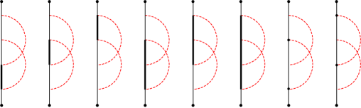
Figure 2.1. The arcs and pairs of points on $\mathcal{Z}$ associated to the generators of $\mathcal{A}=\mathcal{A}(\mathcal{Z},0)$.

The multiplication of two non-trivial generators corresponds to concatenation of the corresponding arcs, which only gives a nontrivial result if the endpoint of the first arc is the same as the starting point of the second. Left (resp. right) compatibility with an idempotent encodes whether the starting point (resp. endpoint) of the subarc contains a point of that idempotent; in other words, for a non-trivial element with starting point $a_{i}$ and ending point $a_{j}$, compatibility on the left with an idempotent is determined by the value of $M(a_{i})$, and compatibility on the right by $M(a_{j})$.

2.2.2. Bordered Heegaard diagrams

Here we lay out the requisite background for bordered Heegaard diagrams and their associated type $A$ and type $D$ structures over $\mathbb{F}_{2}$. Note the definition of these kinds of structures over $\mathbb{F}_{2}$ has the same definition as those over $\mathbb{Z}$ if one ignores the signs. For more details we refer the reader to [bfh2].

Definition 2.6.

A bordered Heegaard diagram is a tuple $\mathcal{H}=(\Sigma,\mbox{\boldmath$\alpha$},\mbox{\boldmath$\beta$},z)$ where

• $\Sigma$ is a compact, oriented surface with one boundary component of genus $g$;

• $\mbox{\boldmath$\beta$}=\{\beta_{1},\dots,\beta_{g}\}$ is a $g$-tuple of pairwise disjoint circles in the interior of $\Sigma$;

• $\mbox{\boldmath$\alpha$}=\{\alpha_{1}^{c},\dots,\alpha_{g-k}^{c},\alpha_{1}^{a},\dots,\alpha_{2k}^{a}\}$ is a $(g+k)$-tuple of pairwise disjoint curves consisting of $g-k$ circles $\mbox{\boldmath$\alpha$}^{c}=\{\alpha_{1}^{c},\dots,\alpha_{g-k}^{c}\}$ in the interior of $\Sigma$ and $2k$ arcs $\mbox{\boldmath$\alpha$}^{a}=\{\alpha_{1}^{a},\dots,\alpha_{2k}^{a}\}$ properly embedded on $\Sigma$ (so $\partial\alpha_{i}^{a}\in\partial\Sigma$ for all $i$);

• $z$ is a point on $\partial\Sigma\setminus(\mbox{\boldmath$\alpha$}\cap\partial\Sigma)$.

There is a pointed matched circle $\mathcal{Z}=(Z,\mathbf{a},M)$ naturally associated to a bordered Heegaard diagram $\mathcal{H}$ with $Z=\partial\Sigma$, $\mathbf{a}=\mbox{\boldmath$\alpha$}\cap\partial\Sigma$, and the matching $M$ given by $M(p)=i$ if only if $p\in\alpha_{i}^{a}\cap\partial\Sigma$. We will sometimes write $\mathcal{Z}$ as $\partial\mathcal{H}$ in this context.

The construction to recover the $3$-manifold with boundary associated to a bordered Heegaard diagram $\mathcal{H}=(\Sigma,\mbox{\boldmath$\alpha$},\mbox{\boldmath$\beta$},z)$ with $\mathcal{Z}=\partial\mathcal{H}$ goes as follows. Begin by taking $[-\epsilon,0]\times Z$ to be a closed collar neighborhood of $\partial\Sigma$ such that $0\times Z$ is identified with $\partial\Sigma$, and also take a tubular neighborhood $Z\times[0,1]$ of $Z$ in $F(\mathcal{Z})$. Now glue $\Sigma\times[0,1]$ to $[-\epsilon,0]\times F(\mathcal{Z})$ by identifying $([-\epsilon,0]\times Z)\times[0,1]\subset\Sigma\times[0,1]$ with $[-\epsilon,0]\times(Z\times[0,1])\subset[-\epsilon,0]\times F(\mathcal{Z})$. Denote the result of this gluing by $Y_{0}$.

Next, attach a 3-dimensional 2-handle to each $\beta_{i}\times 1\subset\Sigma\times[0,1]\subset Y_{0}$ and $\alpha_{i}^{c}\times 0\subset\Sigma\times[0,1]\subset Y_{0}$. We will denote the resulting manifold by $Y_{1}$. Note we now have three boundary components: a sphere $S^{2}$ meeting $\Sigma\times 1$, a surface $\Sigma^{\prime}$ of genus $2k$ meeting $\Sigma\times 0$, and our desired final boundary component given by a surface identified with $0\times F(\mathcal{Z})\subset[-\epsilon,0]\times F(\mathcal{Z})$.

Glue a 3-ball to the $S^{2}$ boundary component, and join each $\alpha_{i}^{a}\times 0\subset\Sigma^{\prime}$ to the co-core of the corresponding handle in $-\epsilon\times F(\mathcal{Z})$ to form a closed curve. Attach a 3-dimensional 2-handle to each of these new circles, and denote the resulting manifold by $Y_{2}$. Then $Y_{2}$ still has a boundary component identified with $F(\mathcal{Z})$, and a $S^{2}$ boundary component meeting $\Sigma\times 0\subset Y_{0}$. Glue a 3-ball to this $S^{2}$ component and the resulting manifold $Y$ is our desired 3-manifold with boundary identified with $F(\mathcal{Z})$. We will occasionally use $\phi$ to notate the identification of $F(\mathcal{Z})$ with $\partial Y$ and write $(Y,\mathcal{Z},\phi)$.

For the purposes of this paper, we restrict the rest of the background discussion to the case of manifolds with torus boundary. We will further restrict to a special class of bordered Heegaard diagrams, called nice diagrams. Nice diagrams are diagrams where each region not containing the basepoint $z$ is either a rectangle or a bigon. As a result, the structure maps for the associated type $A$ or type $D$ structure are encoded in the combinatorics of the diagram. One can show that any bordered 3-manifold admits a nice diagram. Let $\mathcal{H}$ be a nice bordered Heegaard diagram for a bordered manifold $Y$ with torus boundary, and let $\partial\mathcal{H}$ denote the pointed matched circle associated to $\mathcal{H}$. We define the generators for $\mathcal{H}$ to be the subsets of $\mbox{\boldmath$\alpha$}\cap\mbox{\boldmath$\beta$}$ with:

• $g$ total elements

• exactly one element on each closed circle $\beta_{i}$ and exactly one on each $\alpha_{i}^{c}$

• at most one element on each arc $\alpha_{i}^{a}$.

We denote the set of generators for $\mathcal{H}$ by $\mathcal{G}(\mathcal{H})$.

The authors of [bfh2] associate to each generator a $\textrm{spin}^{c}$ structure of the manifold $Y$, and we will write $\mathcal{G}(\mathcal{H},\mathfrak{s})$ to denote the set of generators with a given associated $\textrm{spin}^{c}$ structure $\mathfrak{s}\in\textrm{Spin}^{c}(Y)$. Let $X(\mathcal{H})$ and $X(\mathcal{H},\mathfrak{s})$ be the $\mathbb{F}_{2}$-vector spaces spanned by $\mathcal{G}(\mathcal{H})$ and $\mathcal{G}(\mathcal{H},\mathfrak{s})$ respectively (i.e. $X(\mathcal{H})=\bigoplus_{\mathfrak{s}\in\textrm{Spin}^{c}(Y)}X(\mathcal{H},\mathfrak{s})$). Let $o(\mathbf{x})\in\{1,2\}$ be the index of the $\alpha$-arc occupied by $\mathbf{x}$ and $\overline{o(\mathbf{x})}$ be the index of the unoccupied arc, i.e. the complement of $o(\mathbf{x})$ in $\{1,2\}$. We assume the $\alpha$-arcs are ordered as they appear along $\partial\mathcal{H}$ starting from $z$, so that after identifying $\partial\mathcal{H}$ (or similarly $-\partial\mathcal{H}$) with $\mathcal{Z}$, two points $p,q$ are the endpoints of $\alpha_{i}$ if an only if they are matched in $\mathcal{Z}$ as $M(p)=i=M(q)$. We are now ready to define a right type $A$ structure $\widehat{\mathit{CFA}}(\mathcal{H})$ over $\mathcal{A}(\partial\mathcal{H})$ and a left type $D$ structure $\widehat{\mathit{CFD}}(\mathcal{H})$ over $-\partial\mathcal{H}$.

Given a diagram $\mathcal{H}$, if we identify $\partial\mathcal{H}$ with $\mathcal{Z}$ we can define a right type $A$ structure $\widehat{\mathit{CFA}}(\mathcal{H},\mathfrak{s})$ over $\mathcal{A}$ as follows. Let $\widehat{\mathit{CFA}}(\mathcal{H},\mathfrak{s})$ be the module generated over $\mathbb{F}_{2}$ by $\mathcal{G}(\mathcal{H},\mathfrak{s})$.

Define a right action of $\mathcal{I}$ on $\widehat{\mathit{CFA}}(\mathcal{H},\mathfrak{s})$ by

$$\mathbf{x}\cdot\iota_{t}=\begin{cases}\mathbf{x}\quad\textrm{ if }t=o(\mathbf{x})\\ 0\quad\textrm{otherwise.}\end{cases}$$

It remains to define the $\mathcal{A}_{\infty}$ structure maps $m_{n+1}$. Because we are working in the context of a nice diagram, $m_{n+1}$ is trivial for $n>1$. The map $m_{1}:\widehat{\mathit{CFA}}(\mathcal{H},\mathfrak{s})\mapsto\widehat{\mathit{CFA}}(\mathcal{H},\mathfrak{s})$ counts empty rectangles and bigons in the interior of the surface of $\mathcal{H}$. The map $m_{2}:\widehat{\mathit{CFA}}(\mathcal{H},\mathfrak{s})\otimes_{\mathcal{I}}\mathcal{A}\mapsto\widehat{\mathit{CFA}}(\mathcal{H},\mathfrak{s})$ instead counts empty rectangles with a single edge on the boundary of $\mathcal{H}$ (these are called “half strips” in [bfh2, Section 8]). Specifically $m_{2}(\mathbf{x},\rho_{I})=\mathbf{y}$ if and only if there is an empty rectangle from $\mathbf{x}$ to $\mathbf{y}$ with an edge on $\partial\mathcal{H}$ representing $\rho_{I}$; in addition, $m_{2}(\mathbf{x},\iota_{o(\mathbf{x})})=\mathbf{x}$.

Let $\widehat{\mathit{CFA}}(\mathcal{H})=\bigoplus_{\mathfrak{s}\in\textrm{Spin}^{c}(Y)}\widehat{\mathit{CFA}}(\mathcal{H},\mathfrak{s})$.

Given a diagram $\mathcal{H}$, if we identify $-\partial\mathcal{H}$ with $\mathcal{Z}$ we can define a left type $D$ structure $\widehat{\mathit{CFD}}(\mathcal{H},\mathfrak{s})$ over $\mathcal{A}=\mathcal{A}(-\partial\mathcal{H})$ as follows. Let $\widehat{\mathit{CFD}}(\mathcal{H},\mathfrak{s})$ be the module generated over $\mathbb{F}_{2}$ by $\mathcal{G}(\mathcal{H},\mathfrak{s})$.

Define a left action of $\mathcal{I}$ on $\widehat{\mathit{CFD}}(\mathcal{H},\mathfrak{s})$ by

$$\iota_{t}\cdot\mathbf{x}=\begin{cases}\mathbf{x}\quad\textrm{ if }t=\overline{o(\mathbf{x})}\\ 0\quad\textrm{otherwise.}\end{cases}$$

It remains to define the type $D$ structure map $\delta^{1}:\widehat{\mathit{CFD}}(\mathcal{H},\mathfrak{s})\to\mathcal{A}\otimes_{\mathcal{I}}\widehat{\mathit{CFD}}(\mathcal{H},\mathfrak{s})$. Let

$$\delta^{1}(\mathbf{x}):=\displaystyle\sum_{\mathbf{y}\in\mathcal{G}(\mathcal{H},\mathfrak{s})}\displaystyle\sum_{RECT\in\pi_{2}(\mathbf{x},\mathbf{y})}\iota_{\overline{o(\mathbf{y})}}\otimes\mathbf{y}+\sum_{\mathbf{y}\in\mathcal{G}(\mathcal{H},\mathfrak{s})}\displaystyle\sum_{RECT^{\partial}\in\pi_{2}(\mathbf{x},\mathbf{y})}\rho_{I}\otimes\mathbf{y}.$$

The terms of the form $\iota\otimes\mathbf{y}$ come from a count of empty bigons and rectangles in the interior of the surface of $\mathcal{H}$, and the terms of the form $\rho_{I}\otimes\mathbf{y}$ are from a count of the aforementioned “half-strips”, specifically if their edge on $\partial\mathcal{H}$ corresponds to $\rho_{I}$. Let $\widehat{\mathit{CFD}}(\mathcal{H})=\bigoplus_{\mathfrak{s}\in\textrm{Spin}^{c}(Y)}\widehat{\mathit{CFD}}(\mathcal{H},\mathfrak{s})$.

2.2.3. Gluing

Let $\mathcal{H}_{1}=(\Sigma_{1},\mbox{\boldmath$\alpha$}_{1},\mbox{\boldmath$\beta$}_{1},z_{1})$ and $\mathcal{H}_{2}=(\Sigma_{2},\mbox{\boldmath$\alpha$}_{2},\mbox{\boldmath$\beta$}_{2},z_{2})$ be nice bordered Heegaard diagrams for bordered manifolds $(Y_{1},\mathcal{Z},\phi_{1})$ and $(Y_{2},-\mathcal{Z},\phi_{2})$ with torus boundary, respectively. We can create a closed Heegaard diagram by gluing $\mathcal{H}_{1}$ and $\mathcal{H}_{2}$ along their boundaries according to the marked points of their common pointed matched circle. This diagram

$$\mathcal{H}=\mathcal{H}_{1}\cup_{\partial}\mathcal{H}_{2}=(\Sigma_{1}\cup_{\partial}\Sigma_{2},\mbox{\boldmath$\alpha$}_{1}\cup_{\partial}\mbox{\boldmath$\alpha$}_{2},\mbox{\boldmath$\beta$}_{1}\cup\mbox{\boldmath$\beta$}_{2},z_{1}=z_{2})$$

is a closed Heegaard diagram for $Y_{1}\cup_{\partial}Y_{2}=Y_{1}\cup_{\phi_{2}\circ\phi_{1}^{-1}}Y_{2}=Y$. Now let $\widehat{\mathit{CFA}}(\mathcal{H}_{1})$ be the left type $A$ structure associated to $\mathcal{H}_{1}$ and $\widehat{\mathit{CFD}}(\mathcal{H}_{2})$ be the right type $D$ structure associated to $\mathcal{H}_{2}$. Since $\mathcal{H}_{1}$ and $\mathcal{H}_{2}$ are nice diagrams, these structures are bounded. As proven in [bfh2], we then have

$$\widehat{\mathit{CF}}(\mathcal{H})\cong\widehat{\mathit{CFA}}(\mathcal{H}_{1})\boxtimes\widehat{\mathit{CFD}}(\mathcal{H}_{2}).$$

More specifically, the generators of $\widehat{\mathit{CFA}}(\mathcal{H}_{1})\boxtimes\widehat{\mathit{CFD}}(\mathcal{H}_{2})$ take the form $x:=x_{1}\otimes x_{2}$ where $x_{1}$ is a generator of $\mathcal{H}_{1}$, $x_{2}$ is a generator of $\mathcal{H}_{2}$, and $o(x_{1})\neq o(x_{2})$. Then from our previous discussion, we know that on a nice diagram with torus boundary, $\partial^{\boxtimes}(x_{1}\otimes x_{2})=m_{1}(x_{1})\otimes x_{2}+(-1)^{|x_{1}|}\sum_{j}m_{2}(x_{1},a_{j})\otimes y_{j}$ where $\delta^{1}(x_{2})=\sum_{j}a_{j}\otimes y_{j}$. The first term is counting rectangles and bigons in $\mathcal{H}_{1}$, and the pieces of the second term where $a_{j}=\iota_{x_{2}}$ are counting rectangles and bigons in $\mathcal{H}_{2}$. The remaining terms are counting pairs of half-strips, one in each diagram, with segments on the boundary that each correspond to $a_{j}$. One should think of these half-strips as gluing together in the closed diagram to form a rectangle that crosses the joined boundaries. We refer the reader to [bfh2] for the more general case of diagrams that aren’t nice and boundaries other than the torus.

Finally, one can conclude that because these are isomorphic chain complexes, we have that

$$\widehat{\mathit{HF}}(Y)\cong H_{\ast}(\widehat{\mathit{CFA}}(Y_{1})\boxtimes\widehat{\mathit{CFD}}(Y_{2})).$$

2.2.4. Gradings

In [bfh2], the algebra is graded by a non-abelian group $G$, and so are domains on a bordered Heegaard diagram, whereas a right (resp. left) structure associated to a bordered Heegaard diagram is graded by left (resp. right) cosets in $G$ of the subgroup of gradings of periodic domains. The tensor product is graded by double cosets in $G$, from which one can recover the usual differential grading on Heegaard Floer homology.

We will not need the above gradings in this paper, but only a simpler grading by $\mathbb{Z}/2$. Gradings by $\mathbb{Z}/2$ on bordered Floer homology have appeared in [dec, z2gr, hlw]. We lay out definitions here directly, specializing to the case of torus boundary, and encourage the reader to compare with earlier literature.

The discussion in [dec, Section 3] shows that a $\mathbb{Z}/2$-grading on the torus algebra $\mathcal{A}$ that is a reduction of the $G$-grading and plays well with gradings on modules arising from Heegaard diagrams must be $1$ for both $\rho_{12}$ and $\rho_{23}$. By inspection, one sees that there are two possible such gradings on $\mathcal{A}$, which we will denote by $\mathrm{gr}_{1}$ and $\mathrm{gr}_{2}$; see Table 2.1.

	$\rho_{1}$	$\rho_{2}$	$\rho_{3}$	$\rho_{12}$	$\rho_{23}$	$\rho_{123}$
$\mathrm{gr}_{1}$	$0$	$1$	$0$	$1$	$1$	$1$
$\mathrm{gr}_{2}$	$1$	$0$	$1$	$1$	$1$	$0$

Table 2.1. The two $\mathbb{Z}/2$-grading functions $\mathrm{gr}_{1}$ and $\mathrm{gr}_{2}$ on $\mathcal{A}$.

Recall that the algebra $\mathcal{A}(\mathcal{Z})$ (thought of as a bimodule over itself) can be seen as the left-right type $AA$ bimodule associated to a certain $\beta$-$\alpha$-bordered Heegaard diagram $\mathsf{AZ}(\mathcal{Z})$; see for example [hfmor, Section 4]. Figure 2.2 shows this diagram when $\mathcal{Z}$ the pointed matched circle for a torus. Each generator of $\mathcal{A}=\mathcal{A}(\mathcal{Z},0)$ corresponds to an intersection point of an $\alpha$-curve and a $\beta$-curve, as indicated on Figure 2.2. For example, the idempotent $\iota_{1}$ ($\iota_{2}$ resp.) corresponds to the intersection point in $\alpha_{1}\cap\beta_{1}$ (resp. $\alpha_{2}\cap\beta_{2}$) that lies on the diagonal “edge” of the diagram where 1-handles are attached. The generator $\rho_{1}$ corresponds to the lowest intersection point in $\alpha_{2}\cap\beta_{1}$, as seen on the diagram, and so on. Right and left multiplications correspond to counting $\alpha$-bordered and $\beta$-bordered rectangles, respectively; we omit the complete description here.

Order the $\alpha$-arcs in order of appearance along $\partial(\mathsf{AZ}(\mathcal{Z}))\setminus z$, and order the $\beta$-curves in the same way. Choose an orientation on the $\alpha$-arcs, and orient the $\beta$-arcs identically, so that the intersection signs at points corresponding to idempotents are all positive. The sign function

$$s(\mathbf{x})=\textrm{sign}(\sigma_{\mathbf{x}})\prod_{i=1}^{g}s(x_{i})$$

on generators of $\mathsf{AZ}(\mathcal{Z})$ induces a $\mathbb{Z}/2$ differential grading $m$ on the algebra $\mathcal{A}(\mathcal{Z})$ given by $s=(-1)^{m}$. Here, $\sigma_{\mathbf{x}}$ is the permutation for $\mathbf{x}$ coming from the induced order of the occupied arcs. When $\mathcal{Z}$ is the pointed matched circle for the torus, there are four possible orientations on the curves. When both $\alpha$-arcs are oriented pointing into (or both pointing out of) the Heegaard surface as they first appear along $\partial(\mathsf{AZ}(\mathcal{Z}))\setminus z$, it is easy to see that $m=\mathrm{gr}_{1}$. In the other two cases, we have $m=\mathrm{gr}_{2}$.

$\iota_{1}$ at 115 20 $\rho_{1}$ at 115 52 $\rho_{12}$ at 115 82 $\rho_{123}$ at 115 112 $\iota_{2}$ at 81 51 $\rho_{2}$ at 81 82 $\rho_{23}$ at 81 112 $\rho_{3}$ at 52 112 $\alpha_{1}$ at 180 60 $\beta_{1}$ at 90 187 $\alpha_{2}$ at 180 90 $\beta_{2}$ at 60 187

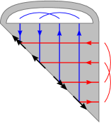
Figure 2.2. The diagram $\mathsf{AZ}(\mathcal{Z})$ when $\mathcal{Z}$ is the pointed matched circle for a torus. Arcs are further oriented, yielding a sign-induced grading $m$ that agrees with $\mathrm{gr}_{1}$.

Given a bordered Heegaard diagram $\mathcal{H}$ of genus $g$ for a manifold with torus boundary, order the $\alpha$-arcs so that $\alpha_{1}^{a}$ is the first arc we encounter starting at $z$ and following the orientation on $\partial\mathcal{H}$, and $\alpha_{2}^{a}$ is the second arc. Also order and orient the $\alpha$ and $\beta$ circles, and define a complete ordering on all $\alpha$-curves by $\alpha^{c}_{1},\ldots,\alpha^{c}_{g-1},\alpha_{1}^{a},\alpha_{2}^{a}$. Write each generator as an ordered tuple $\mathbf{x}=(x_{1},\ldots,x_{g})$ so that

$$x_{1} \in\alpha^{c}_{1}\cap\beta_{\sigma_{\mathbf{x}}(1)}$$

$$\hskip 7.0pt\vdots$$

$$x_{g-1} \in\alpha^{c}_{g-1}\cap\beta_{\sigma_{\mathbf{x}}(g-1)}$$

$$x_{g} \in\alpha_{o(\mathbf{x})}\cap\beta_{\sigma_{\mathbf{x}}(g)}$$

for some permutation $\sigma_{\mathbf{x}}$. For each $x_{i}$, define $s(x_{i})$ to be the intersection sign of $\alpha$ and $\beta$ at $x_{i}$. Last, define the sign of $\mathbf{x}$ by

$$s(\mathbf{x})=\textrm{sign}(\sigma_{\mathbf{x}})\prod_{i=1}^{g}s(x_{i}).$$

We define a $\mathbb{Z}/2$-valued function $m$ on generators of $\mathcal{H}$ by the rule $s=(-1)^{m}$.

Proposition 2.7.

If we choose the grading on $\mathcal{A}(\partial\mathcal{H})$ corresponding to the prescribed orientations of the $\alpha$-arcs near $\partial\mathcal{H}$, the function $m$ is a $\mathbb{Z}/2$ differential grading on $\widehat{\mathit{CFA}}(\mathcal{H})$.

Now, given a bordered Heegaard diagram $\mathcal{H}$ of genus $g$ for a manifold with torus boundary, order the $\alpha$-arcs so that $\alpha_{2}^{a}$ is the first arc we encounter starting at $z$ and following the orientation on $\partial\mathcal{H}$, and $\alpha_{1}^{a}$ is the second arc. Also order and orient the $\alpha$ and $\beta$ circles, and define a complete ordering on all $\alpha$-curves by $\alpha_{1}^{a},\alpha_{2}^{a},\alpha^{c}_{1},\ldots,\alpha^{c}_{g-1}$. Write each generator as an ordered tuple $\mathbf{x}=(x_{1},\ldots,x_{g})$ so that

$$x_{1} \in\alpha_{o(\mathbf{x})}\cap\beta_{\sigma_{\mathbf{x}}(1)}$$

$$x_{2} \in\alpha^{c}_{1}\cap\beta_{\sigma_{\mathbf{x}}(2)}$$

$$\hskip 7.0pt\vdots$$

$$x_{g} \in\alpha^{c}_{g-1}\cap\beta_{\sigma_{\mathbf{x}}(g)}$$

for some permutation $\sigma_{\mathbf{x}}$. For each $x_{i}$, define $s(x_{i})$ to be the intersection sign of $\alpha$ and $\beta$ at $x_{i}$. Last, define the sign of $\mathbf{x}$ by

$$s(\mathbf{x})=(-1)^{o(\mathbf{x})}\textrm{sign}(\sigma_{\mathbf{x}})\prod_{i=1}^{g}s(x_{i}).$$

We define a $\mathbb{Z}/2$-valued function $m$ on generators of $\mathcal{H}$ by the rule $s=(-1)^{m}$.

Proposition 2.8.

If we choose the grading on $\mathcal{A}(-\partial\mathcal{H})$ corresponding to the prescribed orientations of the $\alpha$-arcs near $-\partial\mathcal{H}$, the function $m$ is a $\mathbb{Z}/2$ differential grading on $\widehat{\mathit{CFD}}(\mathcal{H})$.

For brevity, we sometimes write $|\mathbf{x}|$ for $m(\mathbf{x})$.

2.3. Combinatorial sign assignments for closed nice diagrams

In this section, we briefly review the relevant material from [hfz].

Definition 2.9.

A formal generator $\mathbf{x}$ is a one-to-one correspondence $\rho$ between two $n$-element sets $\alpha$ and $\beta$ (which can be represented as a subset of the Cartesian product $\mbox{\boldmath$\alpha$}\times\mbox{\boldmath$\beta$}$), together with a function $\zeta$ from $\rho$ to $\{\pm 1\}$. The set of all such generators will be denoted as $\mathcal{G}_{n}$.

After fixing an ordering of the elements of $\alpha$ and $\beta$, $\mbox{\boldmath$\alpha$}=\{\alpha_{1},\dots,\alpha_{n}\}$ and $\mbox{\boldmath$\beta$}=\{\beta_{1},\dots,\beta_{n}\}$, we can think of the correspondence $\rho$ as the permutation $\sigma\in S_{n}$ for which $\rho=\{(\alpha_{i},\beta_{\sigma(i)})\mid i=1,\ldots,n\}\subset\mbox{\boldmath$\alpha$}\times\mbox{\boldmath$\beta$}$. We can then think of $\zeta$ as the $n$-tuple $\epsilon=(\epsilon_{1},\dots,\epsilon_{n})\in\{\pm 1\}^{n}$ given by $\epsilon_{i}=\zeta(\alpha_{i},\beta_{\sigma(i)})$. We call $\sigma$ and $\epsilon$ the associated permutation and sign profile for the formal generator, and write $\mathbf{x}=(\sigma,\epsilon)$.

Graphically, a formal generator can be thought of as $n$ disjoint crosses between oriented red and blue arcs, with the red arcs decorated with $\alpha_{1},\dots,\alpha_{n}$ and the blue arcs with $\beta_{\sigma(1)},\dots,\beta_{\sigma(n)}$, so that $\alpha_{i}$ and $\beta_{\sigma(i)}$ intersect. The sign profile $\epsilon$ is given by the sign of each cross (with the convention that the $\alpha$-curve comes first). See Figure 2.3 for example.

$\alpha_{1}$ at 73 745 $\beta_{\sigma(1)}$ at 123 745 $\alpha_{2}$ at 162 745 $\beta_{\sigma(2)}$ at 215 745 $\alpha_{3}$ at 251 745 $\beta_{\sigma(3)}$ at 307 745 $\alpha_{4}$ at 341 745 $\beta_{\sigma(4)}$ at 399 745

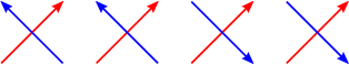
Figure 2.3. A generator with associated permutation $\sigma$ and sign profile $(+1,+1,-1,-1)$.

Definition 2.10.

Fix a positive integer $n$ and sets $\mbox{\boldmath$\alpha$}=\{\alpha_{1},\dots,\alpha_{n}\}$ and $\mbox{\boldmath$\beta$}=\{\beta_{1},\dots,\beta_{n}\}$. Consider $n-1$ disjoint crosses of oriented arcs, along with another pair of oriented arcs, intersecting each other twice and disjoint from all the crosses. The complement of the last two arcs has two components (one compact and one non-compact); the $n-1$ disjoint crosses and the ends of the two arcs that intersect twice are all required to be in the non-compact component. Decorate one of the arcs in each pair of intersecting arcs with an $\alpha_{i}$ and the other one with a $\beta_{j}$ so that each element of $\alpha$ and of $\beta$ is used exactly once. Two such configurations are considered to be equivalent if there is an orientation preserving diffeomorphism of the plane that maps one configuration into the other and respects the orientations and the decorations of the arcs. An equivalence class of such configurations is called a formal bigon. See Figure 2.4 for example.

${\color[rgb]{1,0,0}\alpha_{1}}$ at 3 -2 ${\color[rgb]{0,0,1}\beta_{2}}$ at 60 -2 ${\color[rgb]{1,0,0}\alpha_{2}}$ at 96 -10 ${\color[rgb]{0,0,1}\beta_{3}}$ at 142 -10 ${\color[rgb]{1,0,0}\alpha_{3}}$ at 179 -2 ${\color[rgb]{0,0,1}\beta_{1}}$ at 239 -2 ${\color[rgb]{0,0,0}xy}$ at 29 22 ${\color[rgb]{0,0,0}x}$ at 118 -1 ${\color[rgb]{0,0,0}y}$ at 118 83 ${\color[rgb]{0,0,0}xy}$ at 206 22

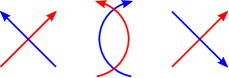
Figure 2.4. An example of a formal bigon. Visually, we can see this bigon goes from the generator $\mathbf{x}=\{(1\ 2\ 3),(+1,+1,-1)\}$ to the generator $\mathbf{y}=\{(1\ 2\ 3),(+1,-1,-1)\}$. See the paragraph after Definition 2.12 for a more precise definition of from and to.

Definition 2.11.

For a fixed positive integer $n$ and sets $\mbox{\boldmath$\alpha$}=\{\alpha_{1},\dots,\alpha_{n}\}$ and $\mbox{\boldmath$\beta$}=\{\beta_{1},\dots,\beta_{n}\}$, consider $n-2$ disjoint oriented crosses. Consider furthermore two pairs of oriented closed arcs ($a_{1},b_{1}$) and ($a_{2},b_{2}$) such that $a_{1}$ and $a_{2}$ (and likewise $b_{1}$ and $b_{2}$) are disjoint, while both $a_{i}$ intersect both $b_{j}$ exactly once in their interiors. One of the two components of the complement of the last four arcs is compact, and we require its interior to be disjoint from all arcs and the endpoints of the four arcs to lie in the non-compact region. Decorate one of the arcs in each pair with an $\alpha_{i}$ and the other one with a $\beta_{j}$ so that each element of $\alpha$ and of $\beta$ is used exactly once, and so that the $a_{i}$ arcs in the rectangle are decorated by elements of $\alpha$ while the $b_{j}$ arcs are decorated with elements of $\beta$. Two such configurations are considered to be equivalent if there is an orientation preserving diffeomorphism of the plane mapping one into the other, while respecting both the orientations and the decorations of the arcs. An equivalence class of such objects is called a formal rectangle. See Figure 2.5 for example.

${\color[rgb]{1,0,0}\alpha_{1}}$ at 3 -6 ${\color[rgb]{0,0,1}\beta_{2}}$ at 60 -6 ${\color[rgb]{1,0,0}\alpha_{2}}$ at 205 5 ${\color[rgb]{0,0,1}\beta_{3}}$ at 96 -12 ${\color[rgb]{1,0,0}\alpha_{3}}$ at 205 63 ${\color[rgb]{0,0,1}\beta_{1}}$ at 186 -12

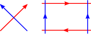
Figure 2.5. An example of a formal rectangle.

Definition 2.12.

A formal flow is either a formal bigon or formal rectangle. For a given integer $n$, the set of all flows moving between elements of $\mathcal{G}_{n}$ will be denoted $\mathcal{F}_{n}$.

The compact region described above for a given formal flow is called the domain for that flow. If we wish to consider the region with its full set of data of both labels and orientations, we refer to it as a decorated domain. A formal flow $\phi$ determines two formal generators $\mathbf{x}$ and $\mathbf{y}$, obtained by adding to the disjoint crosses a small neighborhood of the point(s) where the oriented boundary of the domain switches from a $\beta$-arc to an $\alpha$-arc, or from an $\alpha$-arc to a $\beta$-arc, respectively. We say that $\phi$ is a flow from $\mathbf{x}$ to $\mathbf{y}$, and write $\phi:\mathbf{x}\to\mathbf{y}$. We refer to $\mathbf{x}$ and $\mathbf{y}$ as the starting generator and ending generator, respectively. We call the $\alpha$-indices at which $\mathbf{x}$ and $\mathbf{y}$ differ the moving coordinates. A bigon has one moving coordinate, and the associated generators have identical permutations and sign profiles that differ exactly at that coordinate. A rectangle has two moving coordinates, the generators’ permutations differ by the transposition corresponding to the moving coordinates, and their sign profiles may differ at either both or neither of the moving coordinates and agree elsewhere.

Suppose that the bigons $\phi_{1}$ and $\phi_{2}$ agree at all non-moving coordinates. Furthermore, suppose that at the moving coordinates the $\beta$-arcs both agree or both disagree with the orientation induced by the boundary of the domain, whereas one $\alpha$-arc agrees and the other disagrees with the orientation of the boundary of the domain. Graphically, this means the two domains can be glued along their respective $\alpha$-edges to obtain a disk, so that the labels and orientations of the $\alpha$-arcs match along the gluing, and the $\beta$-arcs result in a consistently oriented and labeled boundary for the disk. We say that $\phi_{1}$ and $\phi_{2}$ are a disk-like $\beta$-type boundary degeneration. See the left diagram in Figure 2.6.

Similarly, suppose that the rectangles $\phi_{1}$ and $\phi_{2}$ agree at all non-moving coordinates, and their domains can be glued along their $\alpha$-arcs to obtain an annulus, so that labels and orientations match along the gluing, and also result in consistently labeled and oriented boundary components for the annulus. We say that $\phi_{1}$ and $\phi_{2}$ are an annular $\beta$-type boundary degeneration. See the right diagram in Figure 2.6.

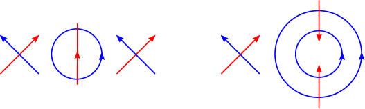
Figure 2.6. Left: A disk-like $\beta$-degeneration in $\mathcal{F}_{3}$. Right: An annular $\beta$-degeneration in $\mathcal{F}_{3}$. Labels on the curves are omitted.

If in the above description the roles of $\alpha$-curves and $\beta$-curves are interchanged, we say that $\phi_{1}$ and $\phi_{2}$ are an $\alpha$-type boundary degeneration.

Observe that in a boundary degeneration, the starting generator of each flow is the ending generator of the other flow.

Now consider a pair of flows $\phi_{1}:\mathbf{x}\to\mathbf{y}$, $\phi_{2}:\mathbf{y}\to\mathbf{z}$, where $\mathbf{x}\neq\mathbf{z}$. Suppose $\phi_{1}$ and $\phi_{2}$ have no moving coordinates in common. This pair uniquely determines another pair of flows $\phi_{3}:\mathbf{x}\to\mathbf{y}^{\prime}$, $\phi_{4}:\mathbf{y}^{\prime}\to\mathbf{z}$ by requiring that $\phi_{3}$ has the same starting generator as $\phi_{1}$ and the same domain (considered with labelings and orientations on the boundary arcs) as $\phi_{2}$, and $\phi_{4}$ has the same ending generator as $\phi_{2}$ and the same domain as $\phi_{1}$. We say that the pairs $(\phi_{1},\phi_{2})$ and $(\phi_{3},\phi_{4})$ form a square. Graphically, this description means that we can embed both domains disjointly in the plane, and complete with crosses in the non-compact region so that all four generators and flows can be seen.

Next suppose $\phi_{1}$ and $\phi_{2}$ share a moving coordinate. We can embed both flows simultaneously on the plane so that the domains have disjoint interiors, there are exactly $n$ red arcs and $n$ blue arcs, and the arcs’ endpoints are all disjoint from the two domains. In this graphical representation, there is a unique way to decompose the union of the domains to see two other flows $\phi_{3}:\mathbf{x}\to\mathbf{y}^{\prime}$, $\phi_{4}:\mathbf{y}^{\prime}\to\mathbf{z}$, so that the union of their domains is the same as that for $\phi_{1}$ and $\phi_{2}$. Suppose further the union of the domains looks like one of the diagrams in Figure 2.7. In this case again we say $(\phi_{1},\phi_{2})$ and $(\phi_{3},\phi_{4})$ form a square.

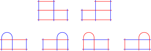
Figure 2.7. Squares. Unlike in Figure 2.6, orientations, as well as crosses at non-moving coordinates are omitted from the diagram. The pairs of flows in the first row examples share one moving coordinate, and there are $n-3$ crosses omitted from each example. The pairs of flows in the second row examples share one moving coordinate, and there are $n-2$ crosses omitted from each example.

We are now ready to recall the definition of a sign assignment.

Definition 2.13.

Fix an integer $n$. A sign assignment of power $n$ is a map $S$ from the set of formal flows $\mathcal{F}_{n}$ to $\{\pm 1\}$ with the following properties:

• if $(\phi_{1},\phi_{2})$ is an $\alpha$-type boundary degeneration, then

  $$S(\phi_{1})\cdot S(\phi_{2})=1;$$

• if $(\phi_{1},\phi_{2})$ is an $\beta$-type boundary degeneration, then

  $$S(\phi_{1})\cdot S(\phi_{2})=-1;$$

• if the two pairs $(\phi_{1},\phi_{2})$ and $(\phi_{3},\phi_{4})$ form a square, then

  $$S(\phi_{1})\cdot S(\phi_{2})=-S(\phi_{3})\cdot S(\phi_{4}).$$

Note that (S-3) can be restated as $\Pi_{i=1}^{4}S(\phi_{i})=-1$.

In [hfz], the authors discuss some additional types of squares $\{(\phi_{1},\phi_{2}),(\phi_{3},\phi_{4})\}$, namely, the ones given by Figure 2.8.

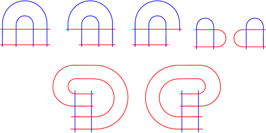
Figure 2.8. Further types of squares.

In [hfz, Lemma 2.8], they show that if $S$ is a sign assignment and $\{(\phi_{1},\phi_{2}),(\phi_{3},\phi_{4})\}$ is one of these further types of squares, then $\Pi_{i=1}^{4}S(\phi_{i})=-1$.

In upcoming arguments, we will occasionally need to compare two rectangles with the same domain but different non-moving coordinates. Two such rectangles are related by a sequence of operations called “simple flips”, defined below.

Definition 2.14.

Let $\phi:\mathbf{x}\to\mathbf{y}$ be a formal rectangle and let $i$ be a non-moving coordinate of $\phi$. Consider the new flow $\phi^{\prime}:\mathbf{x}^{\prime}\to\mathbf{y}^{\prime}$ that has the same domain as $\phi$, and such that $\mathbf{x}^{\prime}$ and $\mathbf{y}^{\prime}$ are obtained from $\mathbf{x}$ and $\mathbf{y}$ by flipping the sign profile at the $i^{\mathrm{th}}$ coordinate. We say that $\phi$ and $\phi^{\prime}$ are related by a simple flip and note that there exists some pair of bigons $b,b^{\prime}$ such that the pairs $(b,\phi)$ and $(\phi^{\prime},b^{\prime})$ form a square.

3. The torus algebra $\mathcal{A}_{\mathbb{Z}}$.

When $\mathcal{Z}$ is the pointed matched circle for the torus, we extend the definition of the summand $\mathcal{A}=\mathcal{A}(\mathcal{Z},0)$ of $\mathcal{A}(\mathcal{Z})$ from Section 2.2.1 to an algebra $\mathcal{A}_{\mathbb{Z}}(\mathcal{Z},0)$.

Definition 3.1.

The (zero-summand) $\mathbb{Z}$-algebra for the pointed matched circle for a torus $\mathcal{A}_{\mathbb{Z}}$ is defined as $\mathcal{A}_{\mathbb{Z}}\coloneqq\mathbb{Z}\otimes_{\mathbb{F}_{2}}\mathcal{A}(\mathcal{Z},0)$.

In other words, we again have eight generators, but over $\mathbb{Z}$, with the same products as for $\mathcal{A}(\mathcal{Z},0)$.

The two functions from Table 2.1 defined on generators extend to $\mathbb{Z}/2$ gradings on $\mathcal{A}_{\mathbb{Z}}$. Thus, there are two distinct graded algebras over $\mathbb{Z}$ that we will consider in this paper. To fit with the diagrammatic nature of sign assignments, we endow a pointed matched circle with additional data, to which a $\mathbb{Z}/2$-graded $\mathbb{Z}$-algebra can naturally be associated. This additional data views each pair of matched points on a pointed matched circle as the boundary of an oriented 1-manifold:

Definition 3.2.

A signed pointed matched circle is a pointed matched circle $\mathcal{Z}=(Z,{\bf a},M,z)$ along with the following data. For each pair of points $M^{-1}(i)$, one point is labelled with $``-"$ and the other is labelled with “$+$”.

Given a pointed matched circle $\mathcal{Z}$, order the $2k$ pairs of points in order of appearance along $\mathcal{Z}\setminus z$. Let $P\in\{-,+\}^{2k}$ be a sign sequence. Define $\mathcal{Z}_{P}$ to be the signed pointed matched circle for which the first point (as encountered along $\mathcal{Z}\setminus z$) of the $i^{\mathrm{th}}$ matched pair is labelled with a $+$ if and only if the $i^{\mathrm{th}}$ coordinate of $P$ is a $+$. For ease of notation, we will write $\mathcal{Z}_{+-}$ for $\mathcal{Z}_{(+,-)}$, and so on.

A signed pointed matched circle $\mathcal{Z}_{P}$ induces an orientation on the $\alpha$- and $\beta$-arcs on $\mathsf{AZ}(\mathcal{Z})$, as follows. Indentify each boundary component of $\mathsf{AZ}(\mathcal{Z})$ with $\mathcal{Z}_{P}$, and orient each arc so it starts at a $-$ and ends at a $+$. We write $\mathsf{AZ}(\mathcal{Z}_{P})$ for the resulting Heegaard diagram along with the prescribed orientations.

When $|{\bf a}|=4$, i.e. in the torus case, there are four distinct signed pointed matched circles – $\mathcal{Z}_{++}$, $\mathcal{Z}_{-+}$, $\mathcal{Z}_{+-}$, and $\mathcal{Z}_{--}$; see Figure 3.1. Observe that the oriented diagram in Figure 2.2 represents $\mathsf{AZ}(\mathcal{Z}_{++})$.

${\color[rgb]{1,0,0}+}$ at -9 24 ${\color[rgb]{1,0,0}+}$ at -9 59 ${\color[rgb]{1,0,0}-}$ at -9 97 ${\color[rgb]{1,0,0}-}$ at -9 132 ${\color[rgb]{1,0,0}1}$ at 50 55 ${\color[rgb]{1,0,0}2}$ at 50 100 ${\color[rgb]{1,0,0}-}$ at 100 24 ${\color[rgb]{1,0,0}+}$ at 100 59 ${\color[rgb]{1,0,0}+}$ at 100 97 ${\color[rgb]{1,0,0}-}$ at 100 132 ${\color[rgb]{1,0,0}1}$ at 160 55 ${\color[rgb]{1,0,0}2}$ at 160 100 ${\color[rgb]{1,0,0}+}$ at 215 24 ${\color[rgb]{1,0,0}-}$ at 215 59 ${\color[rgb]{1,0,0}-}$ at 215 97 ${\color[rgb]{1,0,0}+}$ at 215 132 ${\color[rgb]{1,0,0}1}$ at 272 55 ${\color[rgb]{1,0,0}2}$ at 272 100 ${\color[rgb]{1,0,0}-}$ at 320 24 ${\color[rgb]{1,0,0}-}$ at 320 59 ${\color[rgb]{1,0,0}+}$ at 320 97 ${\color[rgb]{1,0,0}+}$ at 320 132 ${\color[rgb]{1,0,0}1}$ at 385 55 ${\color[rgb]{1,0,0}2}$ at 385 100

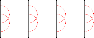
Figure 3.1. The four signed pointed matched circles $\mathcal{Z}_{++}$, $\mathcal{Z}_{-+}$, $\mathcal{Z}_{+-}$, and $\mathcal{Z}_{--}$ (from left to right) for the torus. Here, the top and bottom point on each arc are identified, and represent the basepoint $z$. The circle $Z$ is oriented from bottom to top.

Definition 3.3.

Let $\mathcal{Z}_{P}$ be a signed pointed matched circle for the torus. The $\mathbb{Z}/2$-graded $\mathbb{Z}$-algebra $\mathcal{A}_{P}$ is the algebra $\mathcal{A}_{\mathbb{Z}}$ with the $\mathbb{Z}/2$ grading associated to $\mathsf{AZ}(\mathcal{Z}_{P})$ from Section 2.2.1.

We can see the generators of $\mathcal{A}_{P}$ on $\mathcal{Z}_{P}$ in the same way as in the $\mathbb{F}_{2}$ case in Section 2.2.1. The signed pointed matched circle $\mathcal{Z}_{P}$ and the (unsigned) pointed matched circle $\mathcal{Z}$ have the same underlying data $(Z,{\bf a},M,z)$. An oriented subarc of $Z\setminus z$ with endpoints in ${\bf a}$ corresponds to an element $\rho_{I}$ in $\mathcal{A}_{P}$ if and only if it corresponds to $\rho_{I}$ in $\mathcal{A}$. The ring of idempotents associated to $\mathcal{A}_{P}$ is the algebra $\mathcal{I}_{P}$ generated by the two idempotents of $\mathcal{A}_{P}$. Note that $\mathcal{I}_{P}\cong\mathbb{Z}^{2}$.

If we consider subarcs with the signs on the endpoints inherited from the signed pointed matched circle, one can determine the gradings on the algebra elements in the following way.

Lemma 3.4.

The product of the inherited signs on the endpoints for a subarc $\rho_{I}$ is equal to $(-1)^{\mid\rho_{I}\mid}$.

Proof.

Consider $\mathsf{AZ}(\mathcal{Z}_{P})$. Recall that idempotents always have grading zero, and the grading for $\rho_{I}$ can be determined by comparing the intersection sign at the vertex labelled $\rho_{I}$ with the intersection sign at the idempotent vertex vertically below it: if they agree, $\rho_{I}$ has grading zero; if they differ, it has grading one. By inspection we see that the above signs differ precisely when the two horizontal segments that connect the respective intersection points to the right boundary edge of the diagram have opposing orientations as seen on the diagram. However, we can identify this right boundary component of $\mathsf{AZ}(\mathcal{Z}_{P})$ that intersects the $\alpha$ curves with $\mathcal{Z}_{P}$, and correspondingly view $\rho_{I}$ as an oriented segment on $\mathcal{Z}_{P}$ that connects endpoints of the two horizontal segments discussed above. This in turn tells us that the orientations of these horizontal segments are the same as the orientations (locally speaking) of the $\alpha$-arcs where they intersect the endpoints of $\rho_{I}$ in $\mathcal{Z}_{P}$. Finally, if the orientations of these two $\alpha$-arcs differ, than the inherited signs of the endpoints of $\rho_{I}$ must differ (since those signs are precisely how the orientation is determined in the first place). ∎

4. Bordered Sign Assignments

We now discuss how to extend the construction from [hfz] to bordered Floer homology in the case of torus boundary.

For Definitions 4.2–4.6, fix a positive integer $n$ and a sign sequence $P\in\{-,+\}^{2}$.

Definition 4.1.

A formal right (resp. left) bordered generator is a one-to-one correspondence $\rho$ between two ordered $n$-element sets $\alpha$ and $\beta$ (which can be represented as a subset of the Cartesian product $\mbox{\boldmath$\alpha$}\times\mbox{\boldmath$\beta$}$), together with a function $\epsilon$ from $\rho$ to $\{\pm 1\}$ and a choice $\mathbf{s}\in\{1,2\}$. The choice $\mathbf{s}$ can be thought of as a special label associated to the last (resp. first) element in $\alpha$, as described below. The set of all such generators will be denoted $\mathcal{G}_{n,\mathcal{A}_{P}}^{R}$ (resp. $\mathcal{G}_{n,\mathcal{A}_{P}}^{L}$).

A bordered right (resp. left) generator can be more clearly thought of as $n$ disjoint crosses of oriented arcs. One arc of each cross is labelled by an element of the set $\{\alpha_{1},\dots,\alpha_{n-1},\alpha_{1}^{a},\alpha_{2}^{a}\}$ (resp. $\{\alpha_{1}^{a},\alpha_{2}^{a},\alpha_{2},\dots,\alpha_{n}\}$) so that only one of the two labels $\alpha_{1}^{a}$ and $\alpha_{2}^{a}$ is used, and each $\alpha_{i}$ label is used exactly once. The remaining arcs are labelled by elements of the set $\beta$ so that each element is used once. The choice of $\mathbf{s}$ is the index of the used label $\alpha_{\mathbf{s}}^{a}$. The correspondence $\rho$ can be thought of as the permutation $\sigma\in S_{n}$ represented by the labelling, thinking of the $\alpha_{\mathbf{s}}^{a}$ label as the $n^{\text{th}}$ (resp. first) coordinate of the permutation, and $\epsilon=(\epsilon_{1},\dots,\epsilon_{n})\in\{\pm 1\}^{n}$ is determined by the sign of the crosses, with the convention that the $\alpha$-arcs come first. Once again we call $\sigma$ and $\epsilon$ the associated permutation and sign profile for $\mathbf{x}$, and we call $\mathbf{s}$ the idempotent for $\mathbf{x}$ (see the note below for an explanation). We write $\mathbf{x}=(\sigma,\epsilon,\mathbf{s})$. For clarity, we will frequently write $\sigma_{\mathbf{x}}$ for the permutation $\sigma$ associated to a generator $\mathbf{x}$. Similarly, we will often write $\epsilon(\mathbf{x})$ and $\mathbf{s}(\mathbf{x})$.

We denote the sign profile that is identically $1$ in each factor by ${\bf 1}$.

Note.

Given a specific bordered Heegaard diagram $\mathcal{H}$ and a sign sequence $P\in\{-,+\}^{2}$, one can order and orient all of the $\alpha$-circles, $\beta$-circles, and $\alpha$-arcs so that if we identify $\partial\mathcal{H}$ with $\mathcal{Z}_{P}$, each $\alpha$-arc is oriented from a $+$ to a $-$. With this choice, each generator of the diagram has two associated formal bordered generators, a left one and a right one. For a left (resp. right) generator, we think of the occupied $\alpha$-arc as the “last” (resp. “first”) of all the occupied $\alpha$-curves. The generator is then specified by the associated permutation, the signs of intersections, and the index $\mathbf{s}$ of the occupied $\alpha^{a}$-arc (with the convention that $\alpha_{1}^{a}$ is the first arc we see as we follow $\partial\mathcal{H}$ along the orientation induced as boundary of $\mathcal{H}$, starting at the basepoint $z$). We remark that in the forthcoming definition of the type $A$ structure $\widehat{\mathit{CFA}}(\mathcal{H},\mathbb{Z})$, the choice $\mathbf{s}$ will correspond to the idempotent of $\mathcal{A}_{P}$ which will act on the given generator by the identity.

Definition 4.2.

A formal right (resp. left) internal flow $\phi$ between formal bordered generators $\mathbf{x}$ and $\mathbf{y}$ in $\mathcal{G}_{n,\mathcal{A}_{P}}^{R}$ (resp. in $\mathcal{G}_{n,\mathcal{A}_{P}}^{L}$), is defined analogously to a formal flow from [hfz] (also see Definitions 2.10, 2.11, 2.12)—geometrically it appears the same as in the closed case (a bigon or a rectangle), but the labels now come from $\{\alpha_{1},\dots,\alpha_{n-1},\alpha_{1}^{a},\alpha_{2}^{a}\}$ (resp. $\{\alpha_{1}^{a},\alpha_{2}^{a},\alpha_{2},\dots,\alpha_{n}\}$) and $\beta$ instead of $\alpha$ and $\beta$.

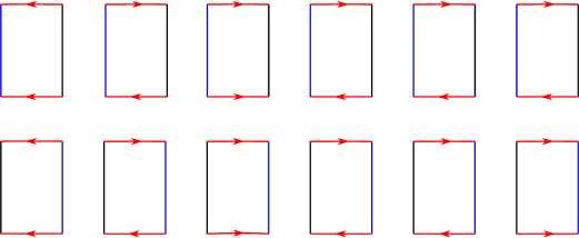
Figure 4.1. Top: The six classes of right bordered flows for the signed pointed matched circle $\mathcal{Z}_{--}$. Bottom: The six classes of left bordered flows for $\mathcal{Z}_{--}$. The non-moving coordinates, as well as the label and orientation of the (blue in this figure) $\beta$-arc at the moving coordinate, are omitted from the figure.

A formal right (resp. left) bordered flow $\phi$ between formal bordered generators in $\mathcal{G}_{n,\mathcal{A}_{P}}^{R}$ (resp. $\mathcal{G}_{n,\mathcal{A}_{P}}^{L}$) is graphically similar to a formal rectangle, but with $n-1$ disjoint crosses and a rectangle. For a right (resp. left) bordered flow, the edges of the rectangle carry the following data when traversed counterclockwise. One edge, hereafter referred to as the bottom edge, has label $\alpha_{i}^{a}$; the next edge, called the right edge, is unlabeled (resp. labeled $\beta_{\sigma(n)}$); the third edge, called the top edge, is labeled $\alpha_{j}^{a}$, with $j$ not necessarily distinct from $i$; the last edge, called the left edge, is labeled $\beta_{\sigma(n)}$ (resp. unlabeled). Label the intersection point of each $\alpha$ arc with the unlabelled edge with a $+$ if the $\alpha$ arc is oriented towards (resp. away from) that point, and with a $-$ if the $\alpha$ arc is oriented away from (resp. towards) that point, and orient the unlabeled edge from bottom to top. We further require that the unlabeled edge with the $\pm$ decorations on it can be identified with an oriented segment of $\mathcal{Z}_{P}\setminus z$ so that the $\pm$ labels match. See Figure 4.1, for example.

The set of flows between elements of $\mathcal{G}_{n,\mathcal{A}_{P}}^{R}$ (resp. $\mathcal{G}_{n,\mathcal{A}_{P}}^{L}$) is denoted $\mathcal{F}_{n,\mathcal{A}_{P}}^{R}$ (resp. $\mathcal{F}_{n,\mathcal{A}_{P}}^{L}$). We call the flows in each set right (resp. left) formal flows.

Note.

Observe that, by definition of formal bordered generator, in a formal internal flow only one of the two $\alpha_{i}^{a}$ labels may be used. Also observe that formal internal flows may carry $\alpha^{a}$-labels at the moving coordinates. Last, note that a right (resp. left) bordered flow has only one moving coordinate, which is the $n^{\text{th}}$ (resp. first) one.

We can further divide right (resp. left) bordered flows into six classes, corresponding to the six non-trivial generators of $\mathcal{A}_{P}$. We say that a bordered flow is of type $\rho_{i}$ if the decorated unlabeled edge, when oriented from bottom to top, agrees with the segment of $\mathcal{Z}_{P}$ representing $\rho_{i}$. In figures, we will often label the “unlabeled” edge with the corresponding $\rho_{i}$.

${\color[rgb]{1,0,0}\alpha_{1}^{a}}$ at 65 855 ${\color[rgb]{1,0,0}\alpha_{2}^{a}}$ at 65 762 ${\color[rgb]{1,0,0}\alpha_{2}^{a}}$ at 150 855 ${\color[rgb]{1,0,0}\alpha_{1}^{a}}$ at 150 762 ${\color[rgb]{1,0,0}\alpha_{1}^{a}}$ at 235 855 ${\color[rgb]{1,0,0}\alpha_{2}^{a}}$ at 235 762 ${\color[rgb]{1,0,0}\alpha_{1}^{a}}$ at 320 855 ${\color[rgb]{1,0,0}\alpha_{1}^{a}}$ at 320 762 ${\color[rgb]{1,0,0}\alpha_{2}^{a}}$ at 405 855 ${\color[rgb]{1,0,0}\alpha_{2}^{a}}$ at 405 762 ${\color[rgb]{1,0,0}\alpha_{1}^{a}}$ at 490 855 ${\color[rgb]{1,0,0}\alpha_{2}^{a}}$ at 490 762 ${\color[rgb]{0,0,0}\rho_{1}}$ at 115 808 ${\color[rgb]{0,0,0}\rho_{2}}$ at 200 808 ${\color[rgb]{0,0,0}\rho_{3}}$ at 285 808 ${\color[rgb]{0,0,0}\rho_{12}}$ at 370 808 ${\color[rgb]{0,0,0}\rho_{23}}$ at 455 808 ${\color[rgb]{0,0,0}\rho_{123}}$ at 540 808 ${\color[rgb]{1,0,0}\alpha_{1}^{a}}$ at 95 743 ${\color[rgb]{1,0,0}\alpha_{2}^{a}}$ at 95 650 ${\color[rgb]{1,0,0}\alpha_{2}^{a}}$ at 180 743 ${\color[rgb]{1,0,0}\alpha_{1}^{a}}$ at 180 650 ${\color[rgb]{1,0,0}\alpha_{1}^{a}}$ at 265 743 ${\color[rgb]{1,0,0}\alpha_{2}^{a}}$ at 265 650 ${\color[rgb]{1,0,0}\alpha_{1}^{a}}$ at 350 743 ${\color[rgb]{1,0,0}\alpha_{1}^{a}}$ at 350 650 ${\color[rgb]{1,0,0}\alpha_{2}^{a}}$ at 435 743 ${\color[rgb]{1,0,0}\alpha_{2}^{a}}$ at 435 650 ${\color[rgb]{1,0,0}\alpha_{1}^{a}}$ at 520 743 ${\color[rgb]{1,0,0}\alpha_{2}^{a}}$ at 520 650 ${\color[rgb]{0,0,0}\rho_{1}}$ at 45 696 ${\color[rgb]{0,0,0}\rho_{2}}$ at 130 696 ${\color[rgb]{0,0,0}\rho_{3}}$ at 215 696 ${\color[rgb]{0,0,0}\rho_{12}}$ at 298 696 ${\color[rgb]{0,0,0}\rho_{23}}$ at 383 696 ${\color[rgb]{0,0,0}\rho_{123}}$ at 465 696

Boundary degenerations and squares for flows in $\mathcal{F}_{n,\mathcal{A}_{P}}^{R}$ or $\mathcal{F}_{n,\mathcal{A}_{P}}^{L}$ are defined analogously to those for the closed case. The only difference is that for squares, some of the geometric configurations in Figure 2.7 (but none of those in Figure 2.8) may now have unlabeled edges instead. See Figure 4.2 for the additional cases.

Definition 4.3.

Suppose that $(\phi_{1},\phi_{2})$ and $(\phi_{3},\phi_{4})$ are distinct pairs of flows, all in $\mathcal{F}_{n,\mathcal{A}_{P}}^{R}$ or all in $\mathcal{F}_{n,\mathcal{A}_{P}}^{L}$, that form a square. If all four flows are internal, we say that $(\phi_{1},\phi_{2})$ and $(\phi_{3},\phi_{4})$ form an internal square. Otherwise, we say that $(\phi_{1},\phi_{2})$ and $(\phi_{3},\phi_{4})$ form a bordered square (see Figure 4.2).

Note that if $(\phi_{1},\phi_{2})$ and $(\phi_{3},\phi_{4})$ form a bordered square, then exactly the first flow in one pair and the second flow in the other pair must be bordered.

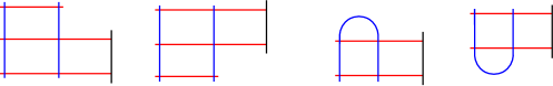
Figure 4.2. Right bordered squares. Left bordered squares can be visualized by reflecting along a vertical line.

Definition 4.4.

Suppose $\phi_{1}$, $\phi_{2}$, and $\phi_{3}$ are right bordered flows with the same label and orientation on the $\beta$-edge of the underlying rectangle, of type $\rho_{i},\rho_{j}$, and $\rho_{k}$, respectively. If $\phi_{2}(\phi_{1}(\mathbf{x}))=\phi_{3}(\mathbf{x})$ and $\rho_{i}\rho_{j}=\rho_{k}\in\mathcal{A}$, we say that the pair $(\phi_{1},\phi_{2})$ and the flow $\phi_{3}$ together form a bordered triangle.

Definition 4.5.

A bordered sign assignment of type $A$, compatible with $P$, and of power $n$ is a map $S_{\mathcal{A}_{P}}^{A}$ from the set of formal flows $\mathcal{F}_{n,\mathcal{A}_{P}}^{R}$ to $\{\pm 1\}$ with the following properties:

• if $(\phi_{1},\phi_{2})$ is an $\alpha$-type boundary degeneration, then

  $$S_{\mathcal{A}_{P}}^{A}(\phi_{1})\cdot S_{\mathcal{A}_{P}}^{A}(\phi_{2})=1;$$

• if $(\phi_{1},\phi_{2})$ is a $\beta$-type boundary degeneration, then

  $$S_{\mathcal{A}_{P}}^{A}(\phi_{1})\cdot S_{\mathcal{A}_{P}}^{A}(\phi_{2})=-1;$$

• if the two pairs $(\phi_{1},\phi_{2})$ and $(\phi_{3},\phi_{4})$ form an internal square, then

  $$S_{\mathcal{A}_{P}}^{A}(\phi_{1})\cdot S_{\mathcal{A}_{P}}^{A}(\phi_{2})=-S_{\mathcal{A}_{P}}^{A}(\phi_{3})\cdot S_{\mathcal{A}_{P}}^{A}(\phi_{4});$$

• if the two pairs $(\phi_{1},\phi_{2})$ and $(\phi_{3},\phi_{4})$ form a bordered square, then

  $$S_{\mathcal{A}_{P}}^{A}(\phi_{1})\cdot S_{\mathcal{A}_{P}}^{A}(\phi_{2})=S_{\mathcal{A}_{P}}^{A}(\phi_{3})\cdot S_{\mathcal{A}_{P}}^{A}(\phi_{4});$$

• if the pair $(\phi_{1},\phi_{2})$ and the flow $\phi_{3}$ form a bordered triangle, then

  $$S_{\mathcal{A}_{P}}^{A}(\phi_{1})\cdot S_{\mathcal{A}_{P}}^{A}(\phi_{2})=S_{\mathcal{A}_{P}}^{A}(\phi_{3}).$$

Note.

The first three properties are analogous to those required of a sign assignment in [hfz], while the remaining two correspond to desired properties of a type $A$ structure. Properties (A-3) and (A-4) say that internal squares anti-commute and bordered squares commute, respectively.

Definition 4.6.

A bordered sign assignment of type $D$, compatible with $P$, and of power $n$ is a map $S_{\mathcal{A}_{P}}^{D}$ from the set of formal flows $\mathcal{F}_{n,\mathcal{A}_{P}}^{L}$ to $\{\pm 1\}$ with the following properties:

• if $(\phi_{1},\phi_{2})$ is an $\alpha$-type boundary degeneration, then

  $$S_{\mathcal{A}_{P}}^{D}(\phi_{1})\cdot S_{\mathcal{A}_{P}}^{D}(\phi_{2})=1;$$

• if $(\phi_{1},\phi_{2})$ is a $\beta$-type boundary degeneration, then

  $$S_{\mathcal{A}_{P}}^{D}(\phi_{1})\cdot S_{\mathcal{A}_{P}}^{D}(\phi_{2})=-1;$$

• if the two pairs $(\phi_{1},\phi_{2})$ and $(\phi_{3},\phi_{4})$ form an internal square, then

  $$S_{\mathcal{A}_{P}}^{D}(\phi_{1})\cdot S_{\mathcal{A}_{P}}^{A}(\phi_{2})=-S_{\mathcal{A}_{P}}^{D}(\phi_{3})\cdot S_{\mathcal{A}_{P}}^{A}(\phi_{4});$$

• if the two pairs $(\phi_{1},\phi_{2})$ and $(\phi_{3},\phi_{4})$ form a bordered square and the bordered flows are of type $\rho$, then

  $$(-1)^{\mid\rho\mid}S_{\mathcal{A}_{P}}^{D}(\phi_{1})\cdot S_{\mathcal{A}_{P}}^{D}(\phi_{2})\cdot S_{\mathcal{A}_{P}}^{D}(\phi_{3})\cdot S_{\mathcal{A}_{P}}^{D}(\phi_{4})=-1;$$

Remark.

Recall that the grading $|\rho|$ depends on the sign sequence $P$.

Definition 4.7.

Let $S$ and $S^{\prime}$ be two bordered sign assignments (both of type $A$ or both of type $D$). We say that $S$ and $S^{\prime}$ are gauge equivalent if there exists a map $u:\mathcal{G}_{n,\mathcal{A}_{P}}\to\{\pm 1\}$ such that for any $\phi\in\mathcal{F}_{n,\mathcal{A}_{P}}$ a formal flow $\phi:\mathbf{x}\to\mathbf{y}$ we have that $S(\phi)=u(\mathbf{x})S^{\prime}(\phi)u(\mathbf{y})$. We also call $u$ a gauge equivalence.

Several distinct gauge equivalence classes of type $A$, as well as of type $D$, bordered sign assignments exist (see Section 5). Further, not every “pairing” of a type $A$ and a type $D$ sign assignment results in a sign assignment in the closed sense. We discuss pairing further in Section LABEL:sec:pairing.

5. Type $A$ sign assignments

5.1. The existence of a type $A$ sign assignment

Our first step in defining a bordered sign assignment $S_{\mathcal{A}_{P}}^{A}$ of type $A$ is to define $S_{\mathcal{A}_{P}}^{A}$ on all formal internal flows. For $\mathbf{s}\in\{1,2\}$, let $\mathcal{G}_{n,\mathcal{A}_{P}}^{\mathbf{s},R}$ be the set of formal right bordered generators of form $(\sigma,\epsilon,\mathbf{s})$. Define two injections $f_{\mathbf{s}}:\mathcal{G}_{n,\mathcal{A}_{P}}^{\mathbf{s},R}\to\mathcal{G}_{n+1}$ as follows.

If $\mathbf{x}=(\sigma,\epsilon,\mathbf{s})$, define $f_{\mathbf{s}}(\sigma)$ to be the permutation that fixes $n+1$ and maps $i$ to $\sigma(i)$ for $i=1,\ldots,n$. Define $f_{\mathbf{s}}(\epsilon)$ as the $(n+1)$-tuple in $\{\pm 1\}^{n+1}$ whose first $n$ coordinates agree with those of $\epsilon$, and whose last coordinate is $1$. Define $f_{\mathbf{s}}(\mathbf{x})=(f_{\mathbf{s}}(\sigma),f_{\mathbf{s}}(\epsilon))$.

Graphically, for $\mathbf{x}\in\mathcal{G}_{n,\mathcal{A}_{P}}^{\mathbf{s},R}$ we think of $f_{\mathbf{s}}(\mathbf{x})$ as the formal generator obtained from $\mathbf{x}$ by replacing the label $\alpha_{\mathbf{s}}^{a}$ with $\alpha_{n}$, and adding one more cross with arcs labeled $\alpha_{n+1}$ and $\beta_{n+1}$ and oriented so their intersection is positive (with the convention that the $\alpha$-arc comes first). See for example Figure 5.1.

$\alpha_{1}$ at 2 100 $\beta_{\sigma(1)}$ at 55 100 $\alpha_{2}$ at 90 100 $\beta_{\sigma(2)}$ at 145 100 $\dots$ at 172 140 $\alpha_{n-1}$ at 195 100 $\beta_{\sigma(n-1)}$ at 250 100 $\alpha_{1}^{a}$ at 285 100 $\beta_{\sigma(n)}$ at 340 100 $\alpha_{1}$ at 2 -10 $\beta_{\sigma(1)}$ at 55 -10 $\alpha_{2}$ at 90 -10 $\beta_{\sigma(2)}$ at 145 -10 $\dots$ at 172 27 $\alpha_{n-1}$ at 195 -10 $\beta_{\sigma(n-1)}$ at 250 -10 $\alpha_{n}$ at 290 -10 $\beta_{\sigma(n)}$ at 340 -10 $\alpha_{n+1}$ at 380 -10 $\beta_{n+1}$ at 440 -10

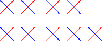
Figure 5.1. Top: A formal bordered generator $\mathbf{x}\in\mathcal{G}_{n,\mathcal{A}_{P}}^{1,R}$. Bottom: The formal generator $f_{1}(\mathbf{x})\in\mathcal{G}_{n+1}$.

Next, we extend the maps $f_{\mathbf{s}}$ to internal flows. Note that if $\phi$ is an internal flow from $\mathbf{x}=(\sigma_{1},\epsilon_{1},\mathbf{s}_{1})$ to $\mathbf{y}=(\sigma_{2},\epsilon_{2},\mathbf{s}_{2})$, then $\mathbf{s}_{1}=\mathbf{s}_{2}$, so simply write $\mathbf{s}$ for $\mathbf{s}_{1}$ or $\mathbf{s}_{2}$. We define $f(\phi)$ as the formal flow from $f_{\mathbf{s}}(\mathbf{x})$ to $f_{\mathbf{s}}(\mathbf{y})$ that is obtained from $\phi$ graphically by relabeling $\alpha_{\mathbf{s}}$ to $\alpha_{n}$ and adding a cross with arcs labeled $\alpha_{n+1}$ and $\beta_{n+1}$ and oriented so their intersection is positive. See for example Figure 5.2.

$\alpha_{1}$ at 2 100 $\beta_{\sigma(1)}$ at 55 100 $\alpha_{2}$ at 90 100 $\beta_{\sigma(2)}$ at 145 100 $\alpha_{3}$ at 185 100 $\beta_{\sigma(3)}$ at 240 100 $\alpha_{1}^{a}$ at 275 100 $\beta_{\sigma(4)}$ at 320 100 $\alpha_{1}$ at 2 -10 $\beta_{\sigma(1)}$ at 55 -10 $\alpha_{2}$ at 90 -10 $\beta_{\sigma(2)}$ at 145 -10 $\alpha_{3}$ at 185 -10 $\beta_{\sigma(3)}$ at 240 -10 $\alpha_{4}$ at 275 -10 $\beta_{\sigma(4)}$ at 320 -10 $\alpha_{5}$ at 360 -10 $\beta_{5}$ at 415 -10

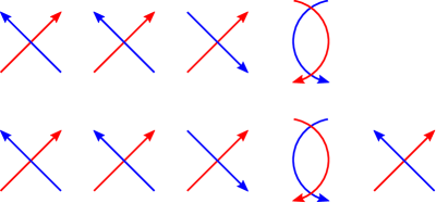
Figure 5.2. Top: A formal internal flow $\phi\in\mathcal{F}_{n,\mathcal{A}_{P}}^{R}$. Bottom: The formal flow $f(\phi)\in\mathcal{F}_{n+1}$. (Here $n=4$.)