Towards Flying through Modular Forms

Abstract

Modular forms are highly self-symmetric functions studied in number theory, with connections to several areas of mathematics. But they are rarely visualized. We discuss ongoing work to compute and visualize modular forms as 3D surfaces and to use these techniques to make videos flying around the peaks and canyons of these “modular terrains.” Our goal is to make beautiful visualizations exposing the symmetries of these functions.

Introduction

We began this project to understand better the shapes of modular forms. A classical modular form is a complex-valued function, defined naturally either on the unit disk or on the half-plane $\mathcal{H}=\{x+iy:x,y\in\mathbb{R},y>0\}$. Each modular form satisfies a set of functional equations of the shape

$$f\left(\frac{az+b}{cz+d}\right)=(cz+d)^{k}f(z),$$ (1)

where $(\begin{smallmatrix}a&b\\ c&d\end{smallmatrix})$ is any matrix in a fixed subgroup $\Gamma\subseteq\mathrm{SL}(2,\mathbb{Z})$ and $k$ is an integer. These functional equations are restrictive and impose a many symmetries on the modular form. Each matrix in $\Gamma$ relates $f(z)$ to another value $f(\frac{az+b}{cz+d})$, but it is hard to grasp how these relations affect the overall shape of the modular form.

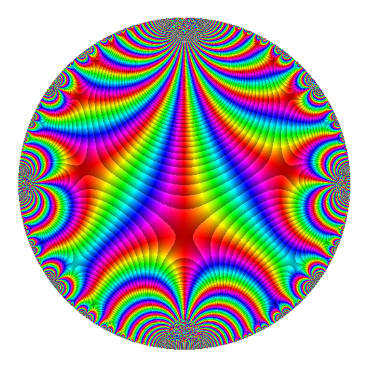
(a)

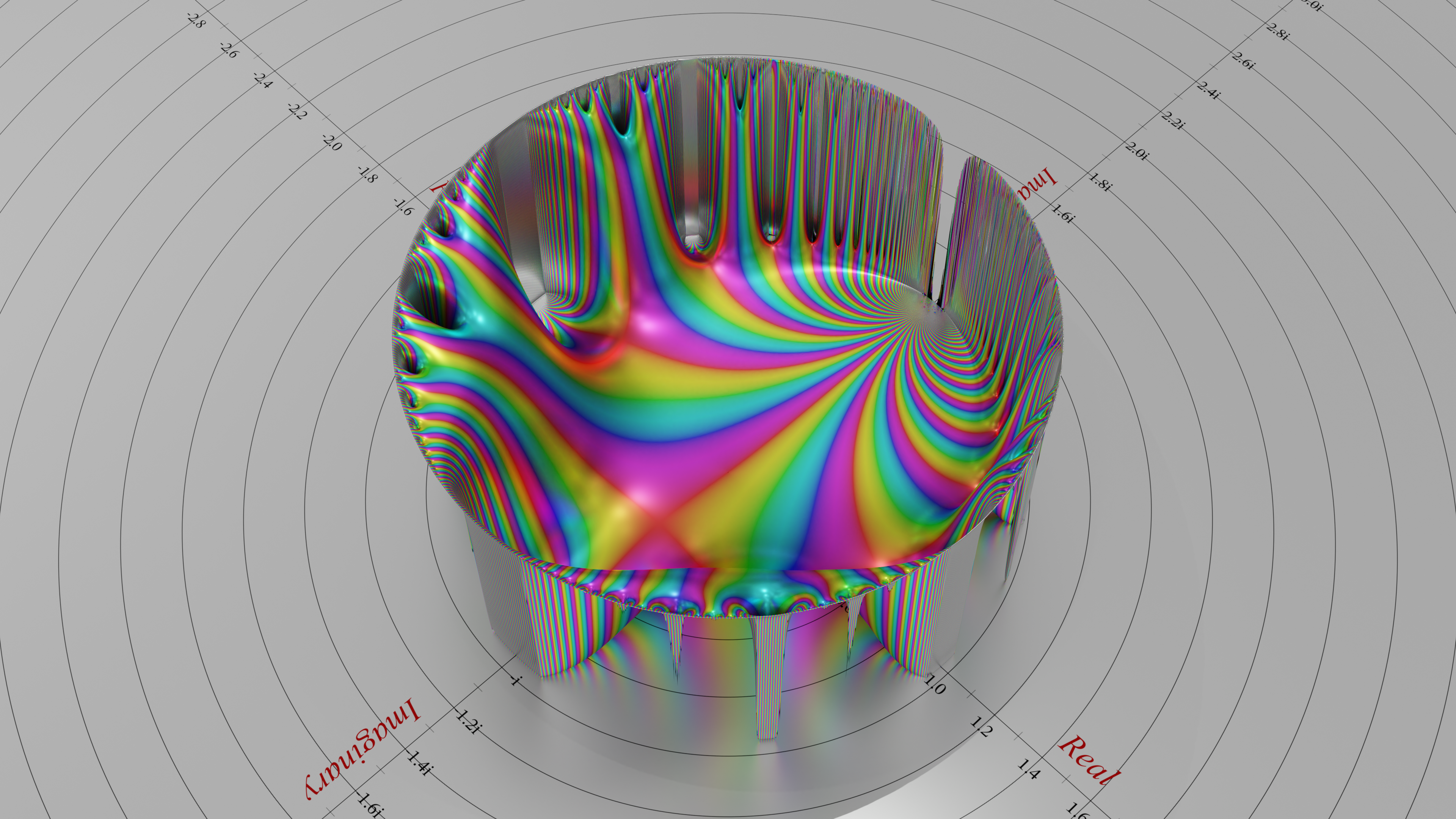
(b)

Figure 1: A modular form in 2D and 3D.

In [5], one of the authors began to study various visualizations of modular forms in detail. Figure 1(a) shows one of the detailed visualizations created. Although a lot of detail is apparent, we find that this doesn’t give a satisfying understanding of the shape of the modular form. In Figure 1(b), we show a particular 3D rendering we created of the same modular form. In this paper, we describe our ongoing efforts to make accurate, informative, and beautiful 3D representations similar to Figure 1(b).

3D Representation of Modular Forms

The fundamental problem of visualizing a modular form, either mentally or with a computer, is that the “obvious” visualization is four-dimensional. Thus when we try to represent a modular form we must carefully choose our representation. This is true for visualizations of all complex functions $f:\mathbb{C}\longrightarrow\mathbb{C}$.

Most visualizations for complex functions descend from some form of domain coloring, a term coined initially in Farris’s review of Visual Complex Analysis [2]. To visualize a function $f$ with domain coloring, you first assign a color to each point of the complex plane. Then you color each point $z$ in the domain of $f$ by the color assigned to the point $f(z)$. Repeated or predictable choices of coloring often lead to understandable visualizations, but it is also possible to deliberately color the plane in a way to emphasize or accentuate behaviors of the visualized function. We’ve drawn particular inspiration from [3] and [6], and hope to explore further color choices in the future.

Our visualizations are 3D domain colorings that we call modular terrains. To each point $z=x+iy$ in the domain, we compute the function $f(z)=re^{i\theta}$ in polar form. We use the magnitude $r$ to determine the height of the surface at the point $(x,y)$, and we use the phase $\theta$ to determine the color of the surface. Finally, we shine a light at the resulting surface to get a better sense of the topography through highlights and shadows.

Different choices of maps from magnitude to height radically alter the appearance of the resulting surface. This is particularly noticeable with modular forms, as the magnitudes will change exponentially, even in small regions. Figures 1(b), 2(a), and 2(b) show three views of the same modular form, each with a different choice of magnitude-to-height function. In Figure 2(a) we used $\tanh(r)$, the hyperbolic tangent function, and then restricted the output to $[0,1]$. This separates “small” and “large” values. In Figure 2(b) we used $\arctan(1/r)$ and then restricted the output to $[0,1]$. But we prefer height maps of the form $\arctan(\log(r^{\alpha}+1))$ for some $\alpha\in(0,1)$. These are the same as the magnitude-to-brightness maps in §2.2.2 of [5]. In Figure 1(b) and later figures, we use $\arctan(\log(\sqrt{r}+1))$. The idea behind these maps is that $\log$ tempers the exponential growth of the magnitudes and $\arctan$ acts like a smooth restriction map, bounding the heights. We chose $\sqrt{r}$ through trial and error, as it gives the terrains gentle, beautiful transitions from lows to highs.

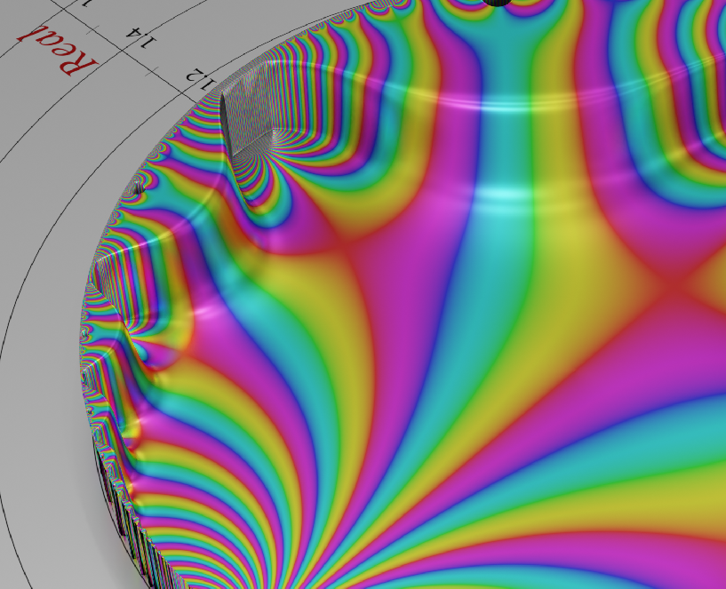
(a)

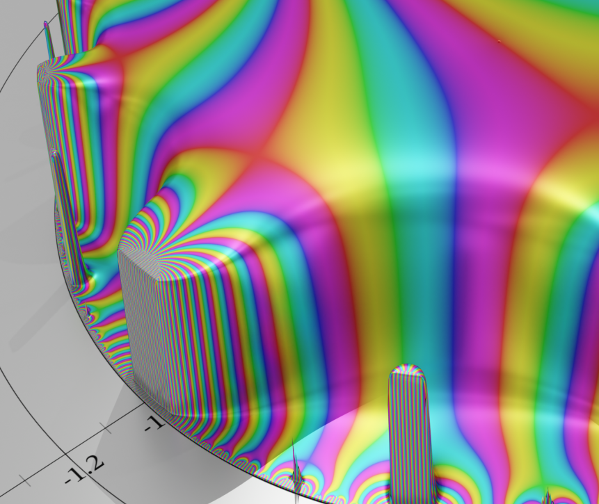
(b)

Figure 2: The same modular form visualized with two different height functions.

We based our color choices on the standard 2D domain coloring, as in Figure 1(a). Color comes from the $\theta$ in $f(z)=re^{i\theta}$. We aligned the color wheel so that red corresponds to $\theta=0$. But we also project a light onto the modular terrains. The shadows and highlights affect the colors, but also serve as visual cues that make the shape more understandable. Although we sought renderings that clearly describe the modular forms, we can also use the modular terrains as a canvas. In Figure 3(d), we “paint” on the modular terrain, making art intrinsically connected to the modular form.

In practice, we compute a triangulation of the surface defined by $f(z)$ and our choice of height function. We rendered all the images in this paper with Blender and used shaders for coloring.

Modular Topography

Perhaps the most studied modular form is the Delta function

$$\Delta(z)=e^{2\pi iz}\prod_{n\geq 1}(1-e^{2\pi inz})^{24}=e^{2\pi iz}-24e^{2\pi i(2z)}+252e^{2\pi i(3z)}+\cdots$$ (2)

Figures 1, 2, and 3 all depict $\Delta(z)$. The Delta function connects work in complex analysis, Riemann surfaces, and algebraic geometry to the theory of elliptic functions. It is the discriminant of the elliptic invariants of the Weierstrass $\wp$ function, and is also called the modular discriminant. Ramanujan investigated $\Delta(z)$ and asked questions leading to the modern theory of modular forms. Our figures depict $\Delta(z)$.

To produce accurate visualizations, we use the self-symmetries from the functional equations (1) to compute each value $\Delta(z)$ in a region where the infinite expansion (2) rapidly converges. In regions where $\Delta(z)$ is extremely small, it is also necessary to perform the computation with higher machine precision to get a smooth surface. This enables close examination of the details around a particular area, even around the “rim,” as in Figure 3. Notice this figure gives three points of view of the same region, as well as a beautiful view with nonstandard coloring. We are working towards producing smooth video transitions across these points of view, giving the impression of flying around the modular terrain.

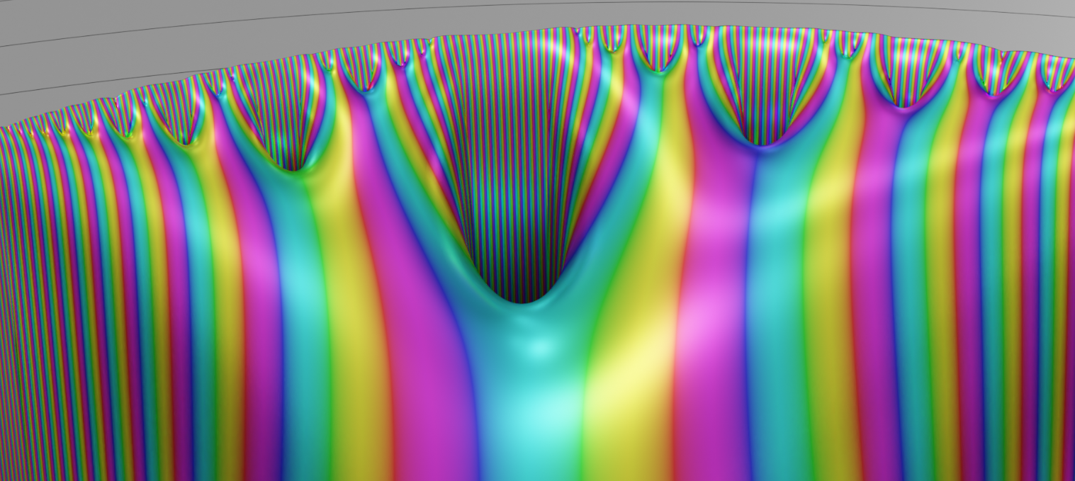
(a)

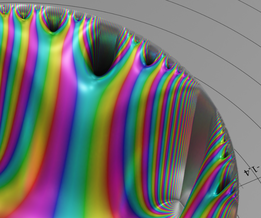
(b)

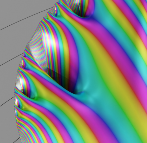
(c)

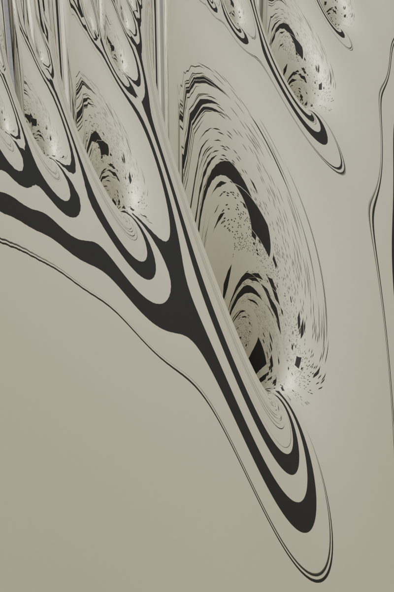
(d)

Figure 3: Four views of the topographic details on the rim of $\Delta(z)$.
In (d), we paint the surface with a periodic generative pattern.

For other modular forms, we can begin with data in the LMFDB [4] (building on the computations in [1]). We’re working on similar techniques for high precision visualization of arbitrary modular forms, but in practice the functional equations (1) are more complicated for different matrix subgroups and precise computation becomes vastly more tedious near the boundary.

Despite these difficulties, we’ve begun to compute modular terrains for different modular forms. In Figure 4(a) we see the modular form 5.4.a.a, and in Figure 4(b) we see the modular form 56.1.h.a. We note that the number and variety of “canyons” visually differ, as does the rate of “elevation change” — and further, we find this much clearer in 3D than in 2D. We look forward to visualizing more modular forms.

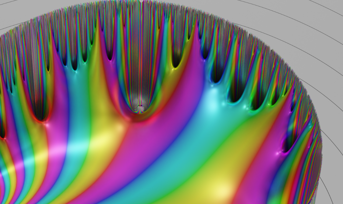
(a)

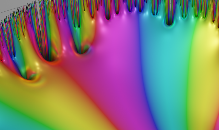
(b)

Figure 4: Detail views of the modular forms 5.4.a.a (a) and 56.1.h.a (b).

Summary and Future Work

We’ve described a set of 3D visualizations and presented several static renderings. In the YouTube video https://www.youtube.com/watch?v=s6sdEbGNdic, we have our first dynamic, flying view of $\Delta(z)$. We’re working on efficient methods of computing visualizations of more modular forms, which we plan on using to make more visualizations. These will appear on the second author’s YouTube channel “The Mathemagicians’ Guild,” https://www.youtube.com/channel/UCHsYWDqJkNlboBpyrRqLzkA. We also plan on making more art with these terrains as canvas, as in Figure 3(d).

References

- [1] A.J. Best, J. Bober, A.R. Booker, E. Costa, J. Cremona, M. Derickx, D. Lowry-Duda, M. Lee, D. Roe, A.V. Sutherland, and J. Voight. “Computing classical modular forms.” To appear in Arithmetic Geometry, Number Theory, and Computation. Simons Symposia series by Springer. Preprint at https://arxiv.org/abs/2002.04717.
- [2] Frank A. Farris. ”A Review of Visual Complex Analysis, by Tristan Needham.” The American Mathematical Monthly, vol. 105, no. 6, 1998, pp. 570–576.
- [3] Frank A. Farris. Creating symmetry: The artful mathematics of wallpaper patterns. Princeton University Press, 2015.
- [4] The LMFDB Collaboration. The L-functions and modular forms database. http://www.lmfdb.org, 2020. [Online; accessed 20 February 2020].
- [5] David Lowry-Duda. “Visualizing Modular Forms.” To appear in Arithmetic Geometry, Number Theory, and Computation. Simons Symposia series by Springer. Preprint at https://arxiv.org/abs/2002.05234.
- [6] Elias Wegert and Gunter Semmler. “Phase plots of complex functions: a journey in illustration.” Notices of the AMS, vol. 58, 2010, pp. 768–780.