Wave manipulation using a bistable chain with reversible impurities

Abstract

We systematically study linear and nonlinear wave propagation in a chain composed of piecewise-linear bistable springs. Such bistable systems are ideal testbeds for supporting nonlinear wave dynamical features including transition and (supersonic) solitary waves. We show that bistable chains can support the propagation of subsonic wavepackets which in turn can be trapped by a low-energy phase to induce energy localization. The spatial distribution of these energy foci strongly affects the propagation of linear waves, typically causing scattering, but, in special cases, leading to a reflectionless mode analogous to the Ramsauer-Townsend (RT) effect. Further, we show that the propagation of nonlinear waves can spontaneously generate or remove additional foci, which act as effective “impurities”. This behavior serves as a novel mechanism for reversibly programming the dynamic response of bistable chains.

I Introduction

Multistable mechanical metamaterials have attracted increasing attention from various research communities in physics, engineering, and materials science, both because of their unique static and dynamic behavior Shan et al. (2015); Rafsanjani et al. (2015); Bertoldi et al. (2017). Indeed, multistability has been leveraged to achieve controlled state changes in engineering applications such as reconfigurable robots Hawkes et al. (2010); Chen et al. (2018), deployable space structures Seffen and Pellegrino (1999), medical devices Kuribayashi et al. (2006), and many others.

Even simple discrete systems composed of bistable elements (i.e., bistable lattices) are capable of rich and varied nonlinear dynamics. For example, by tailoring the energy landscape of a bistable element, a bistable lattice can allow the propagation of transition fronts Nadkarni et al. (2014, 2016); Raney et al. (2016); Jin et al. (2020); Yasuda et al. (2020) where the propagating directions and speed can be manipulated. In addition, recent studies have shown that a bistable chain can support the propagation of solitary waves Katz and Givli (2018, 2019); Vainchtein (2020).

Here, we study the in situ manipulation of the dynamic response of a bistable chain in the broader context of linear/nonlinear wave dynamics. In particular, we showcase a mechanism for controllably inserting reversible effective “impurities” in a bistable chain, arising from the trapping of propagating wavepackets. We numerically investigate the amplitude-dependent behavior of a bistable chain that can support not only supersonic solitary waves but, depending on the impact speed, also subsonically propagating wavepackets. We find that the propagation of the latter is brought to a halt in the bulk of the chain, leading to the formation of effective impurities (albeit within a homogeneous medium) that may play a central role in subsequent dynamics. More specifically, we demonstrate that the presence of such energy foci affects the scattering of linear waves. Interestingly, if two such effective impurities are placed next to each other and the system is driven at a specific frequency that leads to the propagation of a linear wave of a particular wavenumber, complete transmission without reflection can occur in a bistable lattice Martínez et al. (2016). This is reminiscent of the Ramsauer-Townsend (RT) effect, which is well-known in quantum mechanics Sakurai (1994), the simplest instance of which involves the perfect transmission at select energies in one-dimensional scattering from a square well. Multiple impurities can be created via collisions of a propagating wavepacket with an impurity. Note that hereafter we will use the term impurity in this loose sense, implying the presence of a standing wave, even though no spatial inhomogeneity is present in the lattice.

Our presentation is organized as follows: Section II discusses the model setup, explains the dynamic response of a 1D bistable chain under impact excitation, and identifies the formation of impurities due to the trapping of a subsonic wavepacket. In Section III, we investigate the scattering behavior between plane waves and single impurities. Section IV explores scattering for the case with multiple impurities. Finally, Section V summarizes our findings and presents directions for future studies.

Figure 1: (a) Schematic illustration of the system composed of bistable springs. The impact is applied to the left-most unit ($n=1$) by setting an initial velocity. The right-most mass ($n=N$) is connected to a dashpot. (b) The relationship between force and strain of a bistable spring is expressed by a trilinear function [cf. Eq. (1)]. The stiffness parameters are $(K_{I},K_{S},K_{II})=(1,-1,1.5)$ and the strain parameters are $(r_{S},r_{II})=(0.4,1)$. (c) The bistable energy landscape obtained from the trilinear force-strain relationship of panel (b).

II Bistable chains

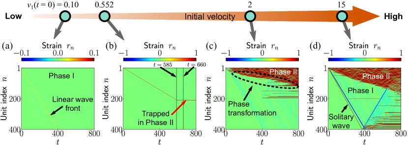
Figure 2: Amplitude-dependent behavior for a bistable chain composed of strain-hardening springs ($K_{II}/K_{I}=1.5$). All unit cells are initially in Phase I. We apply an impact velocity to the first unit cell ($n=1$) by setting $v_{1}(t=0)$. We consider four different values of the impact velocities: (a) $v_{1}(t=0)=0.1$, (b) $0.552$, (c) $2$, and (d) $15$. The color indicates the strain $r_{n}$ as a function of the unit index $n$ and time $t$.

We begin our discussion by examining the dynamic response of a 1D lattice under an elastic impact excitation caused by a striker (see Fig. 1(a)). We define $u_{n}$ as the relative displacement of the $n$th particle measured from its equilibrium point. We define the strain of the $n$th particle as $r_{n}\coloneqq u_{n}-u_{n+1}$. Motivated by the reconfigurability of the bistable lattice we consider the trilinear spring element (see Fig. 1(b)) defined by

$$F(r)=\left\{\begin{array}[]{lcr}{{K}_{I}}r&r\leq r_{a}\\ K_{S}\left(r-r_{S}\right)&r_{a}\leq r\leq r_{b}\\ K_{II}\left(r-r_{II}\right)&r_{b}\leq r\end{array}\right.,$$ (1)

where $K_{I}$, $K_{S}$, and $K_{II}$ are the stiffness parameters. Therefore, Eq. (1) is a double-well potential function as shown in Fig. 1(c). In this study, we use the following set of numerical values for the parameters: $(K_{I},K_{S},K_{II})=(1,-1,1.5)$, and $(r_{S},r_{II})=(0.4,1)$. By using these values, we can determine the other strain parameters $(r_{a},r_{b})$. Here, we define the “Phase I” and “Phase II” regimes corresponding to the stable states around $r_{I}=0$ and $r_{II}=1$, respectively (see also Fig. 1(c)). These two regimes are connected by the spinodal region corresponding to the negative stiffness range (see the shaded gray area in Fig. 1(b)).

Based on this trilinear spring element, the dynamic response of our bistable chain is analyzed by using the following equation of motion:

$${m}{{\ddot{u}}_{n}}=F\left({{u}_{n-1}}-{{u}_{n}}\right)-F\left({{u}_{n}}-{{u}_{n+1}}\right),$$ (2)

where $m$ is the mass of the particle whose value is fixed to $m=1$, and $n=1,\dots,N$ with $N$ being the number of particles in the chain. It should be noted that we can calculate two sound speeds: $c_{I}=\sqrt{K_{I}/m}=1$ and $c_{II}=\sqrt{K_{II}/m}=\sqrt{1.5}$ corresponding to Phase I and Phase II, respectively.

II.1 Amplitude-dependent behavior

We analyze strain profiles of propagating waves in a chain consisting of $N=400$ particles under impact. We numerically simulate the effect of impact by setting the velocity of the first particle to a non-zero value, that is, we set $v_{1}(t=0)\neq 0$. All other initial conditions are set to zero (i.e., positions $u_{n}(t=0)$ and velocities $v_{n}(t=0)$). Then, we advance Eq. (2) forward in time by using a standard fourth-order Runge-Kutta method. To minimize the effect of reflected waves at the other end of the chain ($n=400$), the last particle is connected to a dashpot in which the damping force is linearly proportional to the velocity of the last particle ($F_{\nu}=\nu v_{N}$ with $\nu=1$). The right end of the chain is attached to a rigid wall, i.e., $u_{401}(t)\equiv v_{401}(t)=0\,\,\forall t\geq 0$.

We now discuss Fig. 2 which shows the space-time contour plots of the strain variable for four different values of impact velocities: $v_{1}(t=0)=0.1$, $0.552$, $2$, and $15$. In particular, if $v_{1}(t=0)=0.1$, we only observe small-amplitude wave propagation and the chain configuration remains in Phase I (see Fig. 2(a)). If we increase the impact velocity to $v_{1}(t=0)=0.552$, we observe the formation of a propagating localized wavepacket with amplitude (in the strain variable) greater than $r_{S}=0.4$ (see Fig. 2(b)). This finding indicates that spring elements undergo a transition from Phase I to Phase II and then back to Phase I as the wavepacket propagates in the chain. It is noteworthy that the speed of this excitation ($V_{tw}=0.358$) is slower than that of the small-amplitude wave front (see Fig. 2(a-b)). That is, this is a subsonic propagating wavepacket. Interestingly, this structure is brought to a halt before it reaches the end of the chain, and two adjacent spatial nodes are trapped in Phase II (see the red arrow in Fig. 2(b)), forming the effective impurity discussed above. Note that we observe this trapping behavior for the hardening case (i.e., $K_{II}/K_{I}=1.5$), however, the chain with softening springs (e.g., $K_{II}/K_{I}=0.5$) does not show the formation of impurities or of propagating excitations (see Appendix A for details). Although propagation of supersonic solitary waves in a nonintegrable Fermi-Pasta-Ulam chain Friesecke and Pego (1999); Truskinovsky and Vainchtein (2014), specifically a bistable chain Katz and Givli (2018, 2019); Vainchtein (2020), has been reported previously, the formation of impurities arising from the spontaneous trapping behavior we observe in the present work has been unexplored, to the best of our knowledge.

If $v_{1}(t=0)$ is further increased to $2$, the chain exhibits phase transformation of multiple units which propagate from the left end of the chain to the other end as shown in Fig. 2(c). Finally, when we apply an extremely large amplitude input to the system ($v_{1}(t=0)=15$), we find both propagation of a solitary wave ($V_{tw}=1.076$) and a phase transformation front (see Fig. 2(d)). This solitary wave propagates faster than the (linear) sonic wave speed (i.e., it is a supersonic solitary wave). Therefore, we find that this bistable chain can support coherent structures of both subsonic and supersonic nature, depending on the magnitude of the impact velocity. We will discuss the trapping of subsonically propagating wavepackets in the next section.

II.2 Trapping behavior

Figure 3: Trapping behavior. (a) The spatial distribution of the subsonic wavepacket generated by the impact velocity $v_{1}(t=0)=0.552$ is shown at different instants of time $t$. The waveforms for $t=585$ and $660$ correspond to the black vertical lines in Fig. 2(b), respectively. Each strain profile is shifted in the space domain so that the peak of the strain profile is located at $n=0$ to ease visualization. (b) The strain change of $n=70$ is shown as a function of time $t$. The shaded gray area indicates the spinodal regime (see also Fig. 1(c)). To quantify the wave shape, we measure time widths in which the strain is in the spinodal region, $t_{SpL}$ and $t_{SpR}$, bounded by the red vertical lines. (c) Surface plot of the energy $E_{n}(t)=\frac{1}{2}m\dot{u}_{n}^{2}(t)+U_{n}(t)$ where $U_{n}$ is the bistable potential energy function of Fig. 1(c). (d) The peak energy of the propagating wavepacket is shown as a function of $t$. $\Delta U$ is the energy barrier measured from the energy minimum in Phase II (see Fig. 1(c)). The red vertical line indicates the trapping point at which the peak energy becomes lower than that of the energy barrier $\Delta U$. (e) We calculate the time difference $t_{SpR}-t_{SpL}$, which indicates the symmetric (if $t_{SpR}-t_{SpL}=0$) or asymmetric waveform (otherwise).

To understand this trapping behavior thoroughly, we examine the time evolution of the subsonic propagating wavepacket by extracting the strain waveforms at different time frames, especially right before the trapping occurs. In particular, Fig. 3(a) shows the strain profiles for four different time frames: $t=450$, $520$, $585$, and $660$, (the shapes at $t=585$ and $660$ correspond to the black vertical lines in Fig. 2(b)). Note that the wave profiles are shifted in the spatial domain so that the peak of the wave is located at the center of the domain to ease visualization. The subsonic localized pattern propagates without any noticeable distortions initially (see also Fig. 3(b) for the strain change of $n=70$ as a function of time $t$), although as time passes, the profile features an oscillatory tail as can be discerned at $t=585$ (just before the wave stops) which is denoted by the red dashed ellipse in Fig. 3(a). This tail pattern of the wavepacket stems from its resonance with the linear modes associated with the (zero) background.

Indeed, as the wave propagates the profile loses energy in the form of emitted radiation. This is investigated in panels (c) and (d) of Fig. 3, which depict the spatio-temporal evolution of the total energy of the system and the peak of the energy as a function of time, respectively. As the wave propagates within the chain, the peak energy remains nearly constant, until an abrupt drop in the form of radiation immediately prior to trapping (i.e., when the total energy becomes lower than $\Delta U$, the energy barrier needed to be overcome to return to Phase I). In addition to these energy considerations, we analyze the change of the wave shape by considering the strain in the spinodal region, which is associated with negative stiffness (Fig. 1(b)). To characterize the wave shape, we measure two time widths, $t_{SpL}$ and $t_{SpR}$, in which the strain is in the spinodal region (Fig. 3(b)). We plot the time width difference $t_{SpR}-t_{SpL}$ as shown in Fig. 3(e) in which a positive value of $t_{SpR}-t_{SpL}$ indicates that the strain stays longer in the spinodal region when the unit goes back to the initial state from Phase II. The value of $t_{SpR}-t_{SpL}$ is nearly zero initially (i.e., symmetric wave shape). However, this value increases significantly, most notably right before trapping. This is indicative of rapid growth of distortion. There are two competing processes: 1) potential energy release (and conversion to kinetic) due to the transition from Phase I to Phase II, and 2) potential energy re-balancing from the wavepacket due to its jumping over the energy barrier (and also the spinodal region). The propagation of the subsonic wavepacket shows that these two competing processes are not in the perfect balance needed for genuine traveling. Rather, the energy lost in the form of leakage of radiation wavepackets dominates the energy release, as is evidenced by monitoring the spinodal region. As a result, the wavepacket eventually gets stuck in Phase II, nucleating a new stable phase due to the metastability (cf. Refs. Balk et al. (2001); Ngan and Truskinovsky (2002)). These act effectively as impurities with respect to wave propagation, as described in the next section.

III Scattering between plane waves and impurities

Based on the impurity formation described above, we now turn our focus to the scattering of a plane wave by such impurities in the system. We analyze the propagation of linear waves by considering the following linearized equation of motion posed on an infinite lattice:

$$m{{\ddot{u}}_{n}}={{K}_{n-1}}{{u}_{n-1}}+{{K}_{n}}{{u}_{n+1}}-\left({{K}_{n-1}}+{{K}_{n}}\right){{u}_{n}},$$ (3)

where $K_{n}$ is $K_{II}$ ($K_{I}$) for impurities (rest of the particles). We can thus determine the normal modes of the system by introducing the plane wave ansatz $u_{n}=e^{i\left(kn-\omega t\right)}$ where $k$ and $\omega$ are the wave number and frequency, respectively (with $i=\sqrt{-1}$). Without impurities, we can obtain the customary dispersion relation:

$$\omega=2\pi f=\sqrt{\frac{2K_{I}}{m}\left[1-\cos(k)\right]}.$$ (4)

We systematically study scattering of plane waves by introducing a single impurity (i.e., only a single spring element is in Phase II) or double impurity (two adjacent elements in Phase II) into a host chain in which all elements are initially in Phase I. Figures 4(a) and 4(b) show the schematic illustrations for a chain with a single impurity ($K_{n=0}=K_{II}$) and double impurity ($K_{n=0}=K_{n=1}=K_{II}$).

III.1 Theoretical analysis

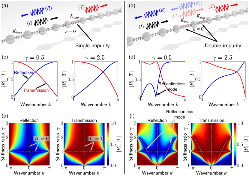
Figure 4: (a-b) Schematic illustrations for a chain with a (a) single and (b) double impurity. Analytical transmission and reflection coefficients for (c) single- and (d) double-impurity cases. The two different stiffness ratio cases (left) $\gamma=0.5$ and (right) $\gamma=2.5$, are shown. The reflection and transmission coefficients for (e) single- and (f) double-impurity cases are plotted as a function of stiffness ratio ($\gamma$) and wavenumber ($k$). The gray dashed lines indicate $|R|=0$ (or $|T|=1$. (e-f)

To examine the effect of impurities on the scattering problem, we employ the following ansatz:

$$u_{n}=\left\{\begin{array}[]{lcr}e^{i(kn-\omega t)}+Re^{-i(kn+\omega t)}\,,&\quad\text{if}&n\leq 0\\ Te^{i(kn-\omega t)}\,,&\quad\text{if}&n>0\end{array}\right.\,,$$ (5)

composed of incident (denoted by $I$ in Fig. 4(a)), reflected ($R$), and transmitted waves ($T$). This way, $|R|^{2}$ and $|T|^{2}$ are the reflection and transmission coefficients, respectively. By following the same procedure used for the granular chain with Hertzian interactions Martínez et al. (2016), we plug Eq. (5) into Eq. (3), and obtain the linear system of equations:

$$\mathbf{Ax}=\mathbf{b},$$ (6)

with

$$\mathbf{A} =\left[\begin{matrix}\gamma{{e}^{ik}}&\frac{{{\omega}^{2}}m}{K_{I}}+{{e}^{ik}}-1-\gamma\\ \left(1+\gamma\right){{e}^{ik}}-{{e}^{2ik}}-\frac{{{\omega}^{2}}m}{K_{I}}{{e}^{ik}}&-\gamma\\ \end{matrix}\right],$$ (7a)

$$\mathbf{x} ={{\left[\begin{matrix}T,&R\\ \end{matrix}\right]}^{T}},$$ (7b)

$$\mathbf{b} ={{\left[\begin{matrix}-\frac{{{\omega}^{2}}m}{K_{I}}+1+\gamma-{{e}^{-ik}},&\gamma\\ \end{matrix}\right]}^{T}},$$ (7c)

for the single-impurity case. Here, we define the stiffness ratio as $\gamma=K_{II}/K_{I}$. Solving Eq. (6) yields respectively the reflection and transmission coefficients:

$${{\left|R\right|}^{2}} ={{\left|\frac{\left(1-\gamma\right)\left(-1+{{e}^{ik}}\right){{e}^{ik}}}{\left(-1+{{e}^{ik}}\right)-2\gamma{{e}^{ik}}}\right|}^{2}},$$ (8a)

$${{\left|T\right|}^{2}} ={{\left|\frac{\gamma\left(1+{{e}^{ik}}\right)}{\left(1-{{e}^{ik}}\right)+2\gamma{{e}^{ik}}}\right|}^{2}}.$$ (8b)

For a chain with a double impurity, we use the following ansatz instead:

$$u_{n}=\left\{\begin{array}[]{lcr}e^{i(kn-\omega t)}+Re^{-i(kn+\omega t)}&\quad\text{if}&n<0\\ {{T}_{1}}{{e}^{i\left(kn-\omega t\right)}}+{{R}_{1}}{{e}^{-i\left(kn+\omega t\right)}}&\quad\text{if}&n=0,1\\ Te^{i(kn-\omega t)}&\quad\text{if}&n>1\end{array}\right..$$ (9)

Here, $|R_{1}|^{2}$ and $|T_{1}|^{2}$ correspond to the reflection and transmission coefficients inside the double-impurity region (see Fig. 4(b)). Then, following the same procedure as above, we arrive at

$$\mathbf{A} =\left[\begin{matrix}0&{{e}^{2ik}}-\left(1+\gamma-\frac{{{\omega}^{2}}m}{K_{I}}\right){{e}^{ik}}&\gamma&\gamma\\ 0&\gamma{{e}^{ik}}&\gamma{{e}^{ik}}-2\gamma+\frac{{{\omega}^{2}}m}{K_{I}}&\gamma{{e}^{-ik}}-2\gamma+\frac{{{\omega}^{2}}m}{K_{I}}\\ {{e}^{2ik}}&0&\gamma-\left(\gamma+1-\frac{{{\omega}^{2}}m}{K_{I}}\right){{e}^{ik}}&\gamma-\left(\gamma+1-\frac{{{\omega}^{2}}m}{K_{I}}\right){{e}^{-ik}}\\ \left(\frac{{{\omega}^{2}}m}{K_{I}}-2\right){{e}^{2ik}}+{{e}^{3ik}}&0&{{e}^{ik}}&{{e}^{-ik}}\\ \end{matrix}\right],$$ (10a)

$$\mathbf{x} ={{\left[\begin{matrix}T,&R,&{{T}_{1}},&{{R}_{1}}\\ \end{matrix}\right]}^{T}},$$ (10b)

$$\mathbf{b} ={{\left[\begin{matrix}\left(-\frac{{{\omega}^{2}}m}{K_{I}}+1+\gamma\right){{e}^{-ik}}-{{e}^{-2ik}},&-\gamma{{e}^{-ik}},&0,&0\\ \end{matrix}\right]}^{T}}.$$ (10c)

In this way, we have

$${{\left|R\right|}^{2}} ={{\left|\frac{\left(1-\gamma\right)\left(-1+{{e}^{ik}}\right)\left\{{{\left(-1+{{e}^{ik}}\right)}^{2}}+2\gamma{{e}^{ik}}\right\}}{-{{e}^{ik}}+\left(3-4\gamma\right){{e}^{2ik}}-3{{\left(1-\gamma\right)}^{2}}{{e}^{3ik}}+{{\left(1-\gamma\right)}^{2}}{{e}^{4ik}}}\right|}^{2}},$$ (11a)

$${{\left|T\right|}^{2}} ={{\left|\frac{{{\gamma}^{2}}\left(1+{{e}^{ik}}\right)}{{{\left(-1+{{e}^{ik}}\right)}^{3}}-2\gamma\left(2-3{{e}^{ik}}+{{e}^{2ik}}\right){{e}^{ik}}+{{\gamma}^{2}}\left(-3+{{e}^{ik}}\right){{e}^{2ik}}}\right|}^{2}}.$$ (11b)

For a single-impurity chain, Fig. 4(c) depicts the reflection (blue) and transmission (red) efficiency for $\gamma=0.5$ (left panel) and $\gamma=2.5$ (right), as a function of the wavenumber $k$. Both stiffness ratio cases show similar monotonic increase (decrease) of the reflection (transmission). On the other hand, the double-impurity case with $\gamma=0.5$ exhibits a non-monotonic change of reflection and transmission. In particular, we find that there exists a reflectionless mode (i.e., the reflection coefficient is identically equal to zero) at a non-zero wavenumber, and complete transmission takes place at that wavenumber, in a way reminiscent of the Ramsauer-Townsend effect. However, if we increase the stiffness value from $\gamma=0.5$ to 2.5, these unique features disappear.

To thoroughly analyze the change of reflection and transmission coefficients, we plot the latter two as a function of the stiffness ratio $\gamma$ and wavenumber $k$. These are shown in Figs. 4(e)-(f) for single- and double-impurity chains, respectively. In these figures, the dashed lines indicate regions with $|R|=0$ or $|T|=1$. The single-impurity chains show monotonic changes of reflection and transmission for any stiffness ratios as we increase or decrease the wavenumber from $k=0$. As far as the double-impurity chains are concerned, our analysis shows an additional minimum reflection valley and transmission peak at non-zero wavenumbers if $\gamma\leq 2$.

III.2 Numerical simulations

Figure 5: Analysis of transmission. (a) Comparison between analytics (black line) and numerics (red markers) for a stiffness ratio of $\gamma=0.5$. (b) Spatio-temporal plots of velocity profiles for excitation frequencies of (left) $\omega=0.6$ and (right) $\omega=1.0$, respectively. The inset shows the temporal dependence of the velocity $v_{n}$ for (gray) $n=-269$ and (red) $n=31$. (c-d) Same as the top panels but for the case corresponding to a double-impurity chain.

We now verify the above theoretical considerations by solving Eq. (2) directly. To draw comparisons between the theoretical analysis and numerical simulations we measure the transmission coefficient numerically by analyzing velocity profiles of incident and transmitted waves under harmonic excitation Martínez et al. (2016). For our numerical computations, we consider $N=601$ particles ($n\in[-300,300]$) and embed an effective impurity. The latter is in the form of a compactly supported nodes at the center of the chain corresponding to $n=0$ for a single-impurity, and $n=0,1$ for a double-impurity. We apply harmonic excitation to the left end of the chain ($n=-300$) in the form of a force input $F_{ex}=F_{0}\sin(\omega t)$ with $F_{0}=10^{-3}$ N. We then calculate the transmission coefficient from numerical simulations, and analyze the velocity profile of the $n=-269$ particle for incident waves and that of the $n=31$ particle for transmitted waves (see Appendix B for details about the calculation of the transmission from direct numerical simulations).

In Fig. 5, we compare theoretical results with numerical simulations for the stiffness ratio $\gamma=0.5$. Figure 5(a) shows the transmission coefficients from numerical simulations (red markers) for the single-impurity case, which demonstrates excellent agreement with the analytical prediction of Eq. (8b) (solid black line). For a single-impurity chain, the reflection coefficient increases with frequency (i.e., wavenumber). In particular, we observe reflected waves with larger amplitude for a value of the excitation frequency of $\omega=1.0$, compared with the case with $\omega=0.6$, as shown in Fig. 5(b). In the case of a double-impurity chain, numerical computations capture a transmission peak at non-zero excitation frequency of about $\omega=1.0$, denoted by the gray arrow in Fig. 5(c). In addition, we observe reflected waves for the $\omega=0.6$ case (see the left panel of Fig. 5(d)), however, such reflected waves are unnoticeable if $\omega=1.0$ is applied to a double-impurity chain (see the right panel of Fig. 5(d)), which corresponds to the reflectionless mode of the RT resonance.

IV Chain with multiple impurities

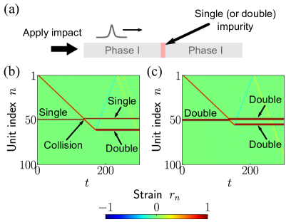
Figure 6: (a) Schematic illustration of a collision of a propagating wavepacket with an impurity. (b-c) Spatio-temporal plots of strain wave profiles for the (b) single and (c) double impurity cases. We apply the initial velocity ($v_{1}(t=0)=0.55$) to the first particle to generate the subsonic propagating wavepacket.

Figure 7: Collision of a (subsonic) propagating wavepacket with a single impurity. (a) Surface plot of the energy $E_{n}(t)=\frac{1}{2}m\dot{u}_{n}^{2}(t)+U_{n}(t)$ where $U_{n}$ is the bistable potential energy function as shown in Fig. 1(c). The red vertical line indicates the collision point. (b) The peak energy of the propagating wavepacket is shown as a function of time.

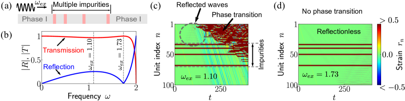
Figure 8: Scattering by multiple double impurities. (a) The schematic illustration highlights the application of a harmonic excitation (with excitation frequency $\omega_{ex}$) to the first unit ($n=1$) of the chain with multiple double impurities. The stiffness parameters for the host and impurities are $K_{host}=1$ and $K_{imp}=1.5$, respectively. (b) The transmission and reflection coefficients for the double impurity with $\gamma=1.5$ are shown as a function of frequency $\omega$. Surface plots of strain wave propagation are presented for: (c) $\omega_{ex}=1.10$ and (d) $\omega_{ex}=1.73$.

With a firm understanding of scattering by single and double effective impurities, we consider now the formation of multiple impurities in the chain and demonstrate an interesting application of the reflectionless mode, specifically for reconfigurable manipulation of linear wave propagation. In Sec. II, we observed the formation of a (double) impurity due to the trapped energy transported by a propagating wavepacket. In this section, we show that the collision of such a wavepacket with an impurity can introduce additional impurities.

To demonstrate this, we perform numerical simulations by generating a propagating wavepacket in a chain with a single or double impurity under impact (see Fig. 6(a)). The stiffness parameters used in this section are $K_{I}=1$ and $K_{II}=1.5$ with an initial velocity of $v_{1}=0.55$ applied to the first particle. This generates a wavepacket as shown in Fig. 6(b) which corresponds to the single-impurity case. We find that a wavepacket penetrates through a single-impurity but its propagation is stopped before reaching the end of the chain, leading to an additional double impurity besides the initial single impurity. Note that the initial impurity is shifted backward by one spatial node. If a wavepacket collides with a double impurity, then an additional double impurity is formed once the solitary wave passes through the impurity region (Fig. 6(c)).

We examine such interactions between a subsonic wavepacket and an impurity by considering the energy change before and after the collisions. In Fig. 7, panel (a) shows the spatio-temporal plot of the total energy $E_{n}$ for the single-impurity case (corresponding to Fig. 6(a)), and we also track the peak energy of the subsonic wavepacket as shown in panel (b). After the collision, some of the energy is reflected (see also the energy decrease of the transmitted wavepacket as shown in panel (b)). However, this reflected energy is not sufficient to generate another propagating wavepacket, and it partly gets trapped causing the backward shift of the impurity, which is followed by the trapping of the transmitted wavepacket. Therefore, our numerical results demonstrate the feasibility of creating multiple impurities via collisions of the propagating wavepacket with impurities, instead of directly manipulating the phase of the individual units.

Having confirmed the formation of multiple impurities in our system, a natural question to ask is whether the reflectionless mode can be observed in a chain with multiple impurities (see Fig. 8(a) for a schematic). Figure 8(b) shows the analytical reflection and transmission coefficients for a chain with multiple double impurities ($\gamma=1.5$) where we identify the reflectionless mode at $\omega=1.73$. To examine the scattering between plane waves and multiple impurities, we consider a chain in which $4$ double impurities are embedded. Then, we apply two different harmonic excitation inputs to the chain for comparison: $\omega_{ex}=1.10$ and $1.73$. Here, the amplitude of excitation force is $F_{0}=0.14$. Figure 8(c) shows the space-time contour plot of strain wave propagation for an excitation frequency of $\omega_{ex}=1.10$. As predicted, we observe the reflected waves. Once these waves reach the left end of the chain, the amplitude of the strain becomes large enough to trigger a phase transition toward Phase II propagating in the chain due to the amplitude-dependent nature of our bistable system. On the other hand, if $\omega_{ex}=1.73$, the wave passes through the impurity region without noticeable reflected waves and no particle overcomes the energy barrier necessary for a phase transition. Once again, our detailed understanding of the scattering problem enables a characterization of the associated reflectionless dynamics within the chain.

V Conclusions & Future Directions

In the present work, we investigated the formation of effective impurities in a bistable chain arising from the trapping of propagating wavepackets formed upon impact. We numerically studied the amplitude dependence of the impact speed on the behavior of linear and nonlinear wave propagation in the bistable chain whose spring elements exhibit an asymmetric energy landscape. In particular, we used numerical simulations to investigate the propagation of wavepackets formed upon impact. Interestingly, our numerical analysis revealed that due to the formation of an oscillatory tail during time propagation, the resulting moving wavepacket loses its energy and eventually gets trapped into a lower energy stationary state.

Based on this emergent localization, we systematically studied the interaction of impurities with linear waves and moving wavepackets. For the linear wave case, we examined the scattering between plane waves and localized structures. In the system with a single impurity, our analytical and numerical results showed that the transmission coefficient monotonically decreases as the harmonic input excitation increases. On the other hand, the bistable chain with two adjacent units in the lower energy phase exhibits a reflectionless mode due to the analog of the well-known Ramsauer-Townsend effect.

Also, we explored the interaction between a single/double impurity and a propagating wavepacket. The latter can pass through the impurity, instead of being reflected or merged into the existing impurity, however, the wavepacket eventually gets trapped in a low-energy state, which creates an additional impurity in the chain. Based on this feasibility of adding multiple impurities, together with the reflectionless mode, we further demonstrated that a phase transition front, or a reflectionless propagation can be “engineered” in the chain with multiple double impurities, depending on the input harmonic frequency. Given that the impurities created by moving wavepackets in a bistable chain can change the linear/nonlinear wave dynamics, such bistable systems can be useful for controlling a reconfigurable structure in a flexible manner. It should be noted in passing that such impurities can be removed from the system by generating the propagation of phase transition fronts Yasuda et al. (2020) (see also Appendix C for numerical demonstrations). This in principle allows reprogramming of the system’s linear dynamic response.

This work paves the path for future efforts. From the theoretical perspective, the analytical derivation of exact traveling solutions in the present setup would be an interesting problem to pursue by using techniques such as those discussed in Refs. Vainchtein (2010); Vainchtein and Kevrekidis (2012) for a diatomic lattice (see also Truskinovsky and Vainchtein (2014)). On the other hand, a systematic existence/bifurcation and stability analysis of traveling waves will be of particular relevance to the present setting. To that end, spectral collocation techniques such as those presented in Ref. Eilbeck and Flesch (1990) could be employed. An especially important aspect of such considerations concerns the nature of the propagating subsonic wavepackets. While these spontaneously emerge as a result of the initial impact, they also shed energy away only to eventually (and spontaneously) transform themselves to compactly supported standing excitations. A further understanding of potential traveling solutions associated with these wavepackets and of the energetics of the above process would be especially useful for the further unveiling of the dynamics of such bistable lattices. Of course, here we have only considered a piecewise linear problem, while realistic systems could be smooth, nonlinear variants thereof. It will be especially interesting to explore which of the ramifications of the present setting (including potential subsonic traveling patterns, compactly supported standing waves and their respective stability traits and scattering implications) are particular to the present setting and which generalize, including, potentially, in higher-dimensional settings. These directions are currently under consideration.

Appendix A: Amplitude-dependent phase transition

Figure A1: Amplitude-dependent phase transition behavior. (a) Schematic illustration for examining the steady-state configuration after an impact is applied to the chain. We extract the final configurations of the chain at $t=3000$ and present them as a function of the impact velocity $v_{1}$ for (b) the softening ($K_{II}/K_{I}=0.5$) and hardening ($K_{II}/K_{I}=1.5$) chains.

To investigate the impact amplitude-dependent phase transition, we conduct numerical simulations on a chain with $100$ particles by applying various amplitude impacts as shown in Fig. A1(a). All of the spring elements are initially in Phase I, and an initial impact is applied to the first particle. Numerical simulations are performed for $t\in[0,3000]$ to allow sufficient time to achieve a steady-state configuration. We demonstrate the final configuration at $t=3000$, representing the steady-state configuration after impact, as a function of the amplitude of impact velocity. The corresponding numerical simulation results for the softening case ($K_{II}/K_{I}=0.5$) are shown in Fig. A1(b), whereas the those for the hardening case ($K_{II}/K_{I}=1.5$) in Fig. A1(c). In the figures, the white and red colors indicate the final states in Phase I and Phase II, respectively. For the softening case, the phase transition tends to be localized around the left end of the chain for smaller amplitude impact, and as we increase the amplitude of the impact input, the phase transition wave propagates in the chain and most of the spring elements move to Phase II states.

For the hardening chain, we obtain more interesting behavior, specifically the formation of a propagating wavepacket. In Fig. A1(c), we find that phase transition occurs only near the left end of the chain for smaller amplitude impact, which is similar to the softening case. However, and in the specific amplitude regime (denoted by the black arrow in the figure), no particle is in Phase II in the final configuration due to the formation of a (subsonic) wavepacket propagating from one end to the other one of the chain. If we increase the impact amplitude from that regime, a (subsonic) wavepacket stops propagating in the middle of the chain, which forms an impurity, as we discussed in Sec. II. Note that when the propagation of a wavepacket is brought to halt, waves propagating toward the left end of the chain are generated (see the red dashed circle in the inset plot of Fig. A1(c)), which sometimes induces phase transition behavior.

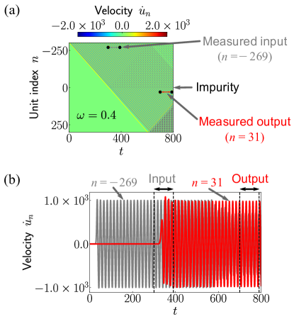
Figure A2: Numerical simulations to obtain the transmission coefficient. (a) Spatio-temporal plot of velocity. We embed a single impurity (stiffness ratio $\gamma=0.5$) in a chain composed of 601 units, and apply harmonic excitation ($\omega=0.4$) to the chain. (b) The temporal distribution of the velocity profiles $v_{n}$ for: (gray) $n=-269$ and (red) $n=31$.

Appendix B: Transmission for various stiffness ratios

Figure A3: Analytical transmission compared with numerical simulations for (a,b) single impurity and (c,d) double impurity cases. We calculate transmission coefficients for various stiffness ratios: (left) $\gamma=1.5$ and (right) $\gamma=2.5$.

Figure A2(a) shows a spatio-temporal plot of particle velocities for the case corresponding to $\omega=0.4$. To calculate the transmission coefficient from numerical simulations, we analyze the velocity profile of the $n=-269$ particle for incident waves and that of $n=31$ particle for transmitted waves. In Fig. A2(b), we present the temporal distribution of the velocity profiles $v_{n}$ for the above mentioned values of $n$ where we calculate the average amplitudes from the steady-state region bounded by the vertical dashed lines. Let $A_{I}$ and $A_{T}$ be the average amplitudes of the incident waves measured at $n=-269$ and transmitted waves at $n=31$. Then, we calculate numerically the transmission as $T_{sim}=A_{T}/A_{I}$.

Besides the case with stiffness ratio $\gamma=0.5$ discussed in Sec. III, we additionally conduct numerical simulations for $\gamma=1.5$ and $2.5$. In Fig. A3, we show numerical results for a chain with (a,b) a single-impurity, and (c,d) a double-impurity. The left (right) two plots are obtained for stiffness ratio of $\gamma=1.5$ ($\gamma=2.5$). Similarly to the comparison for $\gamma=0.5$ in the main text, we confirm excellent agreement between numerical simulation results and analytical transmission coefficients for all four cases.

Appendix C: Impurity disappearance via propagation of phase boundary

Figure A4: Effect of multiple double impurities on phase transitions. Spatio-temporal plots for (a) a homogeneous chain (Phase I) and (b) a chain with double impurities ($K_{imp}=K_{II}=1.5$). We control the displacement of the first unit at constant speed $v_{1}=1.2$. The gray (black) dashed lines indicate the phase boundary (linear wave front). (c) We plot the speed of the phase boundary ($V_{PB}$) as a function of the applied speed $v_{1}$. The inset plot shows the difference between the phase boundary speeds for the homogeneous chain without impurities and the chain with multiple impurities, which is defined as $\Delta V_{PB}=V_{PB}^{i}-V_{PB}^{h}$.

To further reveal the nature of a bistable lattice, we present in this section a way to bring a chain with pre-existing effective impurities to a homogeneous configuration by utilizing the propagation of phase boundaries. To achieve this, we control the displacement of the first particle at constant speed $v_{1}$. The numerical parameters used in our analysis are the same as those of Sec. IV. Figure A4(a) shows the strain profiles for a homogeneous chain in which all spring elements are initially in Phase I. We apply a constant velocity of $v_{1}=1.2$ to the first particle in order to control its displacement. As one can observe in other bistable lattices (e.g., Refs. Slepyan et al. (2005); Truskinovsky and Vainchtein (2006); Deng et al. (2020)), phase transitions from Phase I to Phase II take place and the phase boundary separating the phases (denoted by the gray dashed line) moves at constant speed in the chain. Note that the linear (sonic) waves propagate faster than the phase boundary (see the black dashed line). By embedding multiple double impurities in a host homogeneous chain, we perform the same analysis. In Fig. A4(b), our numerical results show the propagation of phase boundaries in a manner similar to the homogeneous case. These phase transitions bring all spring elements to Phase II. In this way, the bistable chain can achieve a homogeneous configuration (Phase II) without impurities. Although the overall strain profiles for the multiple impurities case is similar to that for the homogeneous case, the propagating phase boundaries experience phase shifts at the locations of the impurities.

To quantify this phase shifting behavior we calculate the speed of the phase boundary propagating in the system by fitting a straight line to the phase boundary (see the gray dashed line in Fig. A4(b)). In Fig. A4(c) the phase boundary speed $V_{PB}$ is presented as a function of the applied velocity for displacement control $v_{1}$. The gray and red markers indicate the phase boundary speed for a homogeneous chain and a chain with multiple impurities, respectively. The solid black line is the analytical phase boundary speed for a homogeneous chain Abeyaratne and Knowles (2006); Zhao and Purohit (2014); Khajehtourian and Kochmann (2020). If the applied velocity is small, we find that the phase boundary speed $v_{PB}$ (obtained from a chain with impurities) is higher than that of the homogeneous case because the linear waves propagate faster in Phase II (impurity locations) due to $K_{II}>K_{I}$. The inset panel in Fig. A4(c) shows the difference between the homogeneous and multiple impurities cases, defined as $\Delta V_{PB}=(V_{PB}^{i}-V_{PB}^{h})/c_{I}$, where $V_{PB}^{h}$ and $V_{PB}^{i}$ are the phase boundary speeds calculated from the homogeneous and multiple impurities cases, respectively. As was already mentioned above, the gap between these two cases is larger for smaller applied velocity and smaller for larger applied velocity, which means that the propagation of phase boundary is insensitive to multiple impurities in a chain. This is due to the fact that the phase boundary speed at high impact velocities approaches the sonic wave speed.

Figure A5: Initialize a chain with multiple impurities under tension. To apply the tension, we control the displacement of the first particle at constant speed $v_{1}$. Spatio-temporal plots of the strain wave profiles for (a) $v_{1}=-0.1$ and (b) $v_{1}=-0.5$.

If we control the displacement of the first particle in the opposite direction it is also possible to bring all spring elements to Phase I. Figure A5 shows the numerical simulation results for two different applied velocities: (a) $v_{1}=-0.1$ and (b) $v_{1}=-0.5$. Interestingly, if the applied velocity is not sufficiently large, the embedded impurities remain in Phase II as shown in Fig. A5(a). However, if $v_{1}=-0.5$, the large-amplitude waves are generated and the impurities are brought back to Phase I. Here, we also observe that the waves experience phase shifts due to impurities.

References

- Shan et al. (2015) S. Shan, S. H. Kang, J. R. Raney, P. Wang, L. Fang, F. Candido, J. A. Lewis, and K. Bertoldi, Advanced Materials 27, 4296 (2015).
- Rafsanjani et al. (2015) A. Rafsanjani, A. Akbarzadeh, and D. Pasini, Advanced Materials 27, 5931 (2015), eprint 1612.05987.
- Bertoldi et al. (2017) K. Bertoldi, V. Vitelli, J. Christensen, and M. Van Hecke, Nature Reviews Materials 2, 17066 (2017).
- Hawkes et al. (2010) E. Hawkes, B. An, N. M. Benbernou, H. Tanaka, S. Kim, E. D. Demaine, D. Rus, and R. J. Wood, Proceedings of the National Academy of Sciences of the United States of America 107, 12441 (2010).
- Chen et al. (2018) T. Chen, O. R. Bilal, K. Shea, and C. Daraio, Proceedings of the National Academy of Sciences of the United States of America 115, 5698 (2018), eprint 1710.04723.
- Seffen and Pellegrino (1999) K. A. Seffen and S. Pellegrino, Proceedings of the Royal Society A: Mathematical, Physical and Engineering Sciences 455, 1003 (1999).
- Kuribayashi et al. (2006) K. Kuribayashi, K. Tsuchiya, Z. You, D. Tomus, M. Umemoto, T. Ito, and M. Sasaki, Materials Science and Engineering: A 419, 131 (2006).
- Nadkarni et al. (2014) N. Nadkarni, C. Daraio, and D. M. Kochmann, Physical Review E 90, 023204 (2014).
- Nadkarni et al. (2016) N. Nadkarni, A. F. Arrieta, C. Chong, D. M. Kochmann, and C. Daraio, Physical Review Letters 116, 244501 (2016).
- Raney et al. (2016) J. R. Raney, N. Nadkarni, C. Daraio, D. M. Kochmann, J. A. Lewis, and K. Bertoldi, Proceedings of the National Academy of Sciences 113, 9722 (2016).
- Jin et al. (2020) L. Jin, R. Khajehtourian, J. Mueller, A. Rafsanjani, V. Tournat, K. Bertoldi, and D. M. Kochmann, Proceedings of the National Academy of Sciences of the United States of America 117, 2319 (2020).
- Yasuda et al. (2020) H. Yasuda, L. M. Korpas, and J. R. Raney, Physical Review Applied 13, 054067 (2020).
- Katz and Givli (2018) S. Katz and S. Givli, Extreme Mechanics Letters 22, 106 (2018).
- Katz and Givli (2019) S. Katz and S. Givli, Physical Review E 100, 32209 (2019).
- Vainchtein (2020) A. Vainchtein, Physical Review E 102, 052218 (2020).
- Martínez et al. (2016) A. J. Martínez, H. Yasuda, E. Kim, P. G. Kevrekidis, M. A. Porter, and J. Yang, Physical Review E 93, 052224 (2016).
- Sakurai (1994) J. Sakurai, Modern Quantum Mechanics (Addison-Wesley, Boston, 1994).
- Friesecke and Pego (1999) G. Friesecke and R. L. Pego, Nonlinearity 12, 1601 (1999).
- Truskinovsky and Vainchtein (2014) L. Truskinovsky and A. Vainchtein, Physical Review E 90, 042903 (2014).
- Balk et al. (2001) A. M. Balk, A. V. Cherkaev, and L. I. Slepyan, Journal of the Mechanics and Physics of Solids 49, 131 (2001).
- Ngan and Truskinovsky (2002) S. C. Ngan and L. Truskinovsky, Journal of the Mechanics and Physics of Solids 50, 1193 (2002), ISSN 00225096.
- Vainchtein (2010) A. Vainchtein, Journal of the Mechanics and Physics of Solids 58, 227 (2010).
- Vainchtein and Kevrekidis (2012) A. Vainchtein and P. Kevrekidis, J Nonlinear Sci 22, 107 (2012).
- Eilbeck and Flesch (1990) J. Eilbeck and R. Flesch, Physics Letters A 149, 200 (1990).
- Slepyan et al. (2005) L. Slepyan, A. Cherkaev, and E. Cherkaev, Journal of the Mechanics and Physics of Solids 53, 407 (2005).
- Truskinovsky and Vainchtein (2006) L. Truskinovsky and A. Vainchtein, SIAM Journal on Applied Mathematics 66, 533 (2006).
- Deng et al. (2020) B. Deng, P. Wang, V. Tournat, and K. Bertoldi, Journal of the Mechanics and Physics of Solids 136, 103661 (2020).
- Abeyaratne and Knowles (2006) R. Abeyaratne and J. K. Knowles, Evolution of Phase Transitions (Cambridge University Press, Cambridge, 2006).
- Zhao and Purohit (2014) Q. Zhao and P. K. Purohit, Modelling and Simulation in Materials Science and Engineering 22, 045004 (2014).
- Khajehtourian and Kochmann (2020) R. Khajehtourian and D. M. Kochmann, Extreme Mechanics Letters 37, 100700 (2020).