Achieving Causality with Physical Clocks

Abstract.

Physical clocks provide more precision than applications can use. For example, a 64 bit NTP clock allows a precision of 233 picoseconds. In this paper, we focus on whether the least significant bits that are not useful to the applications could be used to track (one way) causality among events.

We present PWC (Physical clock With Causality) that uses the extraneous bits in the physical clock. We show that PWC is very robust to errors in clock skew and transient errors. We show that PWC can be used as both a physical and logical clock for a typical distributed application even if just 6-9 extraneous bits (corresponding to precision of 15-120 nanoseconds) are available. Another important characteristic of PWC is that the standard integer $<$ operation can be used to compare timestamps to deduce (one-way) causality among events. Thus, PWC is significantly more versatile than previous approaches for using the physical clock to provide causality information.

1. Introduction

Computer physical clocks often provide precision that is more than what applications can use. For example, a typical clock used by NTP is 64 bits long (RFC0958NTP, ). Of these, the last 32 bits represent a fractional second. In turn, it gives a theoretical resolution of $2^{-32}$ seconds (233 picoseconds). NTPv4 introduces a 128-bit clock of which 64 bits are for the fractional second. Thus, the smallest resolution is $2^{-64}$ seconds (0.05 attoseconds).

For any practical program in a distributed system, these lower-end bits are essentially useless, as they provide a precision that is well below what the application can use. For example, if the execution of an instruction takes $1ns$, any time with finer granularity is meaningless. In fact, for many applications, even larger granularity is sufficient. As an illustration, consider a database application that needs to store the update timestamp of data. In this case, any clock bits that have finer granularity than the time to update an entry are redundant. Or in a monitoring program, if the monitor samples the state of a target application every 100 milliseconds, then granularity finer than $100ms$ is redundant to the monitor. Moreover, if an application is written in Java or Python, then the smallest clock resolution that it could query the system for is 1 nanosecond, and the bits corresponding to values less than $1ns$ are not used. Thus, if we zero out any extraneous bits every time the application uses them, the application would not be affected.

A natural question is whether we can utilize these bits to achieve something useful. In particular, our focus is on using these bits so the physical clock can be simultaneously used as a logical clock (Lamport1974CACM, ). In this case, the information would be useful to clients that are aware of the purpose of these bits, and clients unaware of the purpose of these bits would not be affected.

1.1. Why Incorporate Causality in Physical Clocks

Distributed systems lack a common global clock and processes can only use a local (physical) clock. Since these clocks may grow at their own rate, it presents several challenges that have been identified in the literature.

For example, in Spanner (CDEFFFGGHH13TOCS, ), the authors use tightly synchronized physical clocks to ensure that if we have two transactions $T1$ and $T2$ then the start time of $T2$ is strictly ahead of that of $T1$ even if $T1$ and $T2$ are running on two different machines. This introduces a commit-wait delay, which occurs when $T1$ is writing data that is read by $T2$, but the clock of the machine running transaction $T2$ is lagging.

As another example, GentleRain (GentleRain.DIRZ14SOCC, ) provides causal consistency using 1) partially synchronized physical clocks, and 2) requiring that if the update of variable $x$ happens before the update of variable $y$, then the timestamp of $y$ must be higher than that of $x$ even if $x$ and $y$ are on different machines. To achieve this, the write operation of $y$ needs to be delayed until the clock of the machine hosting $y$ catches up.

If it were guaranteed that physical clock of $f$ was higher than that of $e$ whenever event $f$ is causally dependent on event $e$, these problems would go away. For example, in the Spanner example above, the timestamp of $T2$ would be automatically higher than that of $T1$ thereby obviating the need for a commit-wait delay. CockroachDB has used this approach to eliminate such delays. Likewise, in the case of the GentleRain example, the timestamp of update of $y$ would be automatically higher than that of $x$, thereby eliminating latency in write operations. CausalSpartan (CausalSpartan.RDK17SRDS, ) demonstrated this where they showed that elimination of the write-delay reduces response times to certain queries by an order of magnitude.

Providing physical clocks the ability with to capture causality between events also provides additional avenues to utilize them. For example, using logical clocks, it is possible to take a snapshot of a system in a trivial manner; if each process takes a snapshot when its (logical) clock value is $T$ (a pre-defined value) then the resulting snapshot is consistent. However, the same is not true for (ordinary) physical clock. This ability to take snapshot with logical clocks is not useful in practice as different processes may reach logical clock value $T$ at very different times. On the other hand, an ability to take a snapshot at physical time $T$ would be valuable; it could be used to take a snapshot in the past (e.g., snapshot of the system at 5pm the day before) or in the future (every day at 5pm). This idea is used in (CADK17ICDCS, ) so that we can take snapshots at will, rollback the system to its state a few minutes ago, etc. It has been demonstrated that Retroscope can take up to 150,000 snapshots per second and can be used to monitor a distributed key-value store and perform on-demand rollback without affecting other clients.

A key requirement to allow physical clocks to detect causality is backward compatibility, i.e., the structure of the physical clock (a 64/128 bit integer) should not change. A more complex structure would make it difficult to use them in practice as the clock value is part of several data structures and changing them is not feasible or advisable.

1.2. Prior Approaches

Hybrid logical clocks (HLC) (KDMA2014OPODIS.HLC, ) provide one such approach to enable physical clocks to provide causal information. In (KDMA2014OPODIS.HLC, ), the clock consists of three parts, $pt$, $l$, and $c$, where $pt$ is the physical clock where the event occurred, $l$ is close to the physical clock, and $c$ is a counter whose value is generally very small. In (KDMA2014OPODIS.HLC, ) it is proposed that the last 16 bits of $pt$ are used to store the value of $l-pt$ and the value of $c$ (cf. Figure 1). With this approach, a client who is aware of this encoding can decode to obtain values of $l$ and $c$ that are needed to compare causality between events. While we discuss the details of HLC in the next section, we note that one disadvantage of this approach is that applications that use these clocks need extra work to identify the precise value of $l$ and $c$ before they can be used.

Figure 1. Format of 64-bit Hybrid Logical Clock of an event at process $j$

1.3. Our Approach

Our focus in this paper is to develop a new type of clock, denoted as PWC, physical clock with causality. The goal of PWC is to begin with a parameter u that identifies the extraneous/useless/redundant bits and develop a clock that can be simultaneously used as a physical clock as well as a logical clock. Furthermore, we want to obviate the need for encoding and decoding when comparing timestamps, i.e., we should simply use integer comparison to compare two clock values to identify which value is larger. No decoding/encoding should be necessary beyond applying bitmasks.

Contributions of the paper. We begin in a system where physical clocks of processes are within $\epsilon$ of each other, where $\epsilon$ is a given parameter. This parameter is not known to processes but is only required for ensuring correctness. We develop PWC, using a second parameter u, which identifies the number of extraneous least-significant bits that are available. PWC has the following features.

• It can be used as a substitute for the physical clock. Specifically, for any process $j$, the value of $\textsf{pwc}.j$ is close to the physical clock of $j$.

• It can be used as a substitute for a logical clock. Specifically, for any two events $e$ and $f$, if event $e$ causally affects $f$ (cf. Section 2) then $\textsf{pwc}.e<\textsf{pwc}.f$, where $<$ is the standard “less than” relation between integers.

• PWC can be customized based on the number of useless/ extraneous bits that are available. PWC can be adapted to situations where sufficient extraneous bits are unavailable or the number of extraneous bits needs to be changed dynamically. It is resilient to errors in the clock synchronization protocol.

• We analyze PWC and find that PWC can be used as physical clock and logical clock even in applications that require a very fine clock resolution (tens of nanoseconds). This implies that PWC can be used in virtually any application. By contrast, HLC (KDMA2014OPODIS.HLC, ) cannot be used in applications that need such fine-grained clock resolution. Thus, PWC is more versatile than HLC.

Organization of the paper. The rest of the paper is organized as follows: In Section 2, we define distributed systems, clock synchronization, and causality. We also identify the assumptions made in the paper. In Section 3, we define PWC and identify conditions under which the available extraneous bits are sufficient so that PWC can be used as a substitute for physical clock and logical clock. In Section 4, we discuss the reliability of PWC. In Section 5, we implement a simulated network environment and test the behavior of PWC, followed by a similar experiment on a physical network. We discuss several questions associated with PWC in Section 6. We discuss related work in Section 7 and conclude in Section 8. For reasons of space, proofs, and additional discussions are in the Appendix.

2. Preliminaries

2.1. Distributed Systems

We consider a distributed system that consists of $N$ processes communicating via messages. The state of a process is changed by (send/receive or local) events. Each event is associated with a timestamp. Ideally, the timestamp of an event is the time the event occurs in absolute (global) time. However, absolute time is not practical since it requires infinitesimal granularity and it is not possible to have perfect clock synchronization among processes.

In practice, the timestamp associated with an event comes from the reading of the local clock of the machine/processor/process on which the event occurs. Processes use a protocol such as Network time protocol (NTP) (RFC0958NTP, ; RFC5905NTPv4, ) or Precision Time Protocol (PTP) (ieee1588-2002PTP, ) to keep their local clock synchronized to a master clock and avoid the possibility of arbitrary clock skew due to hardware errors and other failures. We abstract this property by the requirement that clocks of two processes differ by at most $\epsilon$. The value of $\epsilon$ is anywhere between sub-microsecond to several milliseconds based on network size and connectivity. Hence, we make the following assumption:

Assumption 1. There exists a bound $\epsilon$ such that the physical clocks of two processes differ by at most $\epsilon$.

We note that the value of $\epsilon$ is not required to be known to processes. The PWC algorithm does not use it in the implementation; it is needed only for the correctness requirement of PWC algorithm.

The transmission of a message $m$ from $j$ to $k$ can be divided into three time intervals: the message $m$ is sent by originating process $j$ to its network interface card, $m$ is transmitted over the communication network, and $m$ is delivered to target process $k$ from its corresponding network interface card. Those time intervals are denoted as send time, transmit time, and receive time, respectively. We make the following assumption about those time intervals:

Assumption 2. Let $\delta_{se},\delta_{re},\delta_{tr},$ and $\delta_{loc}$ denote the minimum time required to send a message, receive a message, transmit a message, and complete the tasks in a local event. We assume that each of these terms is greater than $0$.

2.2. Causality

Let $e$ and $f$ be two events. We say that event $e$ happens before event $f$, denoted as $e$ $\longrightarrow$ $f$, if and only if: (1) $e$ and $f$ are events on the same process and $e$ occurred before $f$, or (2) $e$ is a send event and $f$ is the corresponding receive event, or (3) There exists an event $g$ such that $e\longrightarrow g$ and $g\longrightarrow f$. We say $e$ and $f$ are concurrent, denoted as $e\|f$, where $e\|f\iff\neg(e\longrightarrow f)\wedge\neg(f\longrightarrow e)$.

A computation of a program is obtained by a partial order of the system’s events such that the order respects causality. As an example, consider the computation shown in Figure 2. Figure 2(a) considers the traditional view of events in distributed computing where events are thought of as instantaneous. In practice, they take some non-zero time. For example, Figure 2(b) shows the timeline of (a subset of) events from Figure 2(a).

(a) Example of Abstract Computation

(b) Example of Concrete Computation

Figure 2. Example of Computation.

2.3. HLC

In this section we provide a brief overview of hybrid logical clocks (KDMA2014OPODIS.HLC, ). In hybrid logical clocks, each process $j$ maintains $pt.j$, which is the physical clock (system clock) of $j$, $l.j$ and $c.j$. The value of $pt.j$ is updated automatically by protocols such as NTP so that, at any given time, $|pt.j-pt.k|$ is bounded by clock skew $\epsilon$ for any two processes $j$ and $k$.

While the detailed algorithm from (KDMA2014OPODIS.HLC, ) is provided for completeness in Appendix, the key observations from (KDMA2014OPODIS.HLC, ) are that (1) for any event $e$, $0\leq l.e-pt.e\leq\epsilon$, and (2) the value of $c.e$ is bounded. In theory, the bound on $c$ is linear in $n$, the number of processes, and $\epsilon$. However, in practice, it is typically small. For this reason, in (KDMA2014OPODIS.HLC, ), it is proposed that the HLC timestamp can be saved as shown in Figure 1. Here, in the 64-bit NTP timestamp, the last 16 bits are used to save the value of $l-pt$ (typically 12 bits) and $c$ (typically 4 bits).

3. PWC Algorithm

In this section, we describe our algorithm to capture causality using the extraneous bits, denoted by u, in the physical clock. This section is organized as follows: Section 3.1 describes the algorithm. Since the algorithm requires sufficient extraneous bits to be available, Section 3.2 identifies sufficient conditions on the required number of extraneous bits. Subsequently, in Sections 3.3 and 3.4, we show that PWC can be used as a substitute for logical clock and physical clock respectively.

3.1. PWC Algorithm

We use the term clpt.j to denote the clock of a process or event $j$ where the extraneous u bits are masked to $0$. We assume that each process $j$ begins with the first event, say $e$ such that $\textsf{pwc}.j=\textsf{pwc}.e=\textsf{clpt}.e$.

In our algorithm, each process $j$ maintains a variable $\textsf{pwc}.j$ that keeps track of the timestamp of $j$ as well as the timestamp of the most recent event on $j$. To create a local event or to send a message, it increments the pwc value by $1$. It also takes a maximum of the pwc value with clpt value. This timestamp is piggybacked on any message $m$ sent by the process, and is denoted as $\textsf{pwc}.m$. The receive operation also works similarly. $\textsf{pwc}.j$ is set to be larger than the old value of $\textsf{pwc}.j$, $\textsf{pwc}.m$ and at least equal to $\textsf{clpt}.j$ (the physical clock of $j$ with extraneous bits reset to $0$). Thus, our algorithm is as follows:

Result: Compute pwc value for newly created event $e$

Initialization: $\textsf{pwc}.j=\textsf{clpt}.j$

if $e$ is a local event then

       $\textsf{pwc}.j=max(\textsf{pwc}.j+1,\textsf{clpt}.j)$;

      

end if

if $e$ corresponds to sending of message $m$ then

       $\textsf{pwc}.j=max(\textsf{pwc}.j+1,\textsf{clpt}.j)$;

       $\textsf{pwc}.m=\textsf{pwc}.j$;

      

end if

if $e$ corresponds to receiving a message $m$ with timestamp $\textsf{pwc}.m$ then

       $\textsf{pwc}.j=max(\textsf{pwc}.j+1,\textsf{pwc}.m+1,\textsf{clpt}.j)$;

      

end if

$\textsf{pwc}.e=\textsf{pwc}.j$;

Algorithm 1 Capturing causality with Extraneous Bits in Physical Clock

Note that clpt and pwc are represented in the same format as an NTP clock rather than as a floating point value as in some standard libraries. Conversion to other formats can be done in the same manner as done for NTP clocks.

3.2. Sufficient Conditions for viability of Algorithm 1

Our next goal is to identify under what conditions can Algorithm 1 be viable. To define the notion of viability, we view the timestamp pwc to consist of two parts: hpt and lpt. The least significant u bits are used for lpt whereas the remaining bits are used for hpt.

The key idea in defining viability is that the bits represented by lpt are irrelevant as far as the physical clock is concerned. PWC permits lpt to be higher than $0$. As long as this value does not overflow, we can use the proposed timestamp. Note that if this value overflows then it would affect hpt, and it would impact the process as it would effectively change the physical clock being seen by the process. With this intuition, we focus on defining the notion of viability, next. We begin with the following assumption.

Assumption 3. We assume that the number of extraneous bits is greater than $0$, i.e., $\textsf{u}>0$.

Assumption 4. We assume that the value of u is constant and identical across all processes during a computation. We consider the case where this value is changed dynamically in Section 6.6.

Assumption 5. In the initial discussion, we assume that physical clock of process $j$ is monotonic. We consider the issue of non-monotonic clocks in Section 6.7.

Assumption 6. The number of events created on process $j$ for a given $\textsf{hpt}.j$ value is bounded, i.e., for any $t$, $|\{e|e$ is an event on $j$ and $\textsf{hpt}.e=t\}|$ is bounded by a constant. For sake of simplicity, we assume that this bound is 1. We note that if this bound is $K$ then $\lceil\log_{2}K\rceil$ bits of lpt would be needed to distinguish such events thereby reducing the extraneous bits. Thus, for any two consecutive events $e$ and $f$ on process $j$, we have $\textsf{hpt}.e<\textsf{hpt}.f$

We note that the impact of this assumption can be reduced by allowing broadcast messages where a node sends multiple messages simultaneously if all these events are timestamped with the same timestamp. Likewise, if a process receives multiple messages simultaneously, then those receive messages can be combined into one receive event. In our implementation, we do not consider this optimization. Using such an optimization would improve applicability of PWC by reducing the number of extraneous bits required for correctness

Finally, the next assumption combines clock skew assumption 2.1 and requirement of finite time spent in each event. Specifically,

Assumption 7. We assume that if absolute time $\epsilon$ has passed between events $e$ and $f$ then $\textsf{hpt}.e<\textsf{hpt}.f$

Based on the definition of hpt and clpt, $\textsf{clpt}.e=2^{\textsf{u}}\cdot\textsf{hpt}.e$. Thus, we have

Observation 1. Let $e$ and $f$ be two consecutive events on process $j$. Then, based on Assumptions 3.2 and 3.2, we have

$\textsf{clpt}.e+2^{\textsf{u}}\leq\textsf{clpt}.f$

$\textsf{clpt}.e+1\leq\textsf{clpt}.f$

Observation 2. If clocks were perfectly synchronized then for any event $e$, lpt.e = 0

For reasons of space, we have kept proofs in Appendix.

If clocks are not perfectly synchronized then the value of lpt could be higher than $0$. In this case, we can make the following observation:

Lemma 1. If there exists an event $f$ such that $\textsf{lpt}.f>0$ then there exists an event $e$ such that $e$ happened before $f$ and $\textsf{pwc}.e=\textsf{pwc}.f-1$

We can generalize this observation recursively. Specifically, if $\textsf{lpt}.f=5$ it implies that there is an event with timestamp $\textsf{pwc}.f-1$. For this event, lpt value is 4. Thus, there is another event with timestamp $\textsf{pwc}.f-2$ ($\textsf{lpt}=3$) and so on. Thus, we have

Lemma 2. If there exists an event $f$ such that $\textsf{lpt}.f=v>0$ then there exists events $e_{1},e_{2},\cdots e_{v}$,

• $\forall w:1\leq w<v:e_{w}\longrightarrow e_{w+1}$

• $\forall w:1\leq w\leq v:\textsf{pwc}.e_{w}=\textsf{pwc}.f-v+(w-1)$

• $e_{v}\longrightarrow f$

Lemmas 3.2 and 3.2 deal with the case when $\textsf{lpt}.f$ is greater than $0$. They state that if $\textsf{lpt}.f$ is greater than $0$ then there is an event $e$ whose (entire) timestamp (i.e., $\textsf{pwc}.e$) is exactly one less than that of $f$ (i.e., $\textsf{pwc}.f$). The reverse may, however, not be true. Specifically, it is possible that there exists an event $f$ such that $\textsf{lpt}.f=0$ and there exists an event $e$ such that $e$ happened before $f$ and $\textsf{pwc}.e+1=\textsf{pwc}.f$. Such a situation can arise if the last u bits of $\textsf{pwc}.j+1$ (or $\textsf{pwc}.m+1$) happen to be all $0$’s. Essentially, in this case, there is an overflow in the lower u bits thereby affecting the significant bits (i.e., bits that were not considered extraneous). With this intuition (and based on Observation 3.2), we define consecutive causal chain. Specifically, a consecutive causal chain is $e_{1},e_{2},\cdots,e_{r}$ such that for any $0<w<r$, $e_{w}\longrightarrow e_{w+1}$, $\textsf{pwc}.e_{w}+1=\textsf{pwc}.e_{w+1}$.

Definition 1. A sequence of events $e_{1},e_{2},\cdots,e_{r}$ is a consecutive causal chain (CCC) iff for each $w,1\leq w<r:$

• $e_{w}\longrightarrow e_{w+1}$

• $\textsf{pwc}.e_{w}+1=\textsf{pwc}.e_{w+1}$

We note that in a consecutive causal chain $e_{1},e_{2},\cdots,e_{r}$, we cannot insert an event in between two events. In other words, we cannot insert event $f$ such that $e_{w}\longrightarrow f\longrightarrow e_{w+1}$. This is straightforward by Theorem 3.3 (cf. Section 3.3) as there is no available timestamp for the event $f$. We can only extend a consecutive causal chain by adding an event at the beginning or at the end. Hence, we define maximal consecutive causal chain (MCCC) to be the one that cannot be extended further on either end. Note that to extend $e_{1},e_{2},\cdots,e_{r}$, we either need an event $e_{0}$ such that $\textsf{pwc}.e_{0}=\textsf{pwc}.e_{1}-1$ and $e_{0}\longrightarrow e_{1}$ or an event $e_{r+1}$ such that $\textsf{pwc}.e_{r+1}=\textsf{pwc}.e_{r}+1$ and $e_{r}\longrightarrow e_{r+1}$.

Definition 2. Algorithm 1 has an overflow in assigning timestamps in a computation $\sigma$ iff $\sigma$ contains events $e,f$ such that $e\longrightarrow f$ and Algorithm 1 assigns timestamps such that $\textsf{pwc}.f=\textsf{pwc}.e+1$, and $\textsf{lpt}.f=0$.

Note that the above definition is conservative. In other words, if there is no overflow in the computation it would imply that hpt is not affected by the increment of lpt. The reverse is not necessarily true.

Definition 3. We say that the deployment of Algorithm 1 in a given system is viable iff for any valid computation (i.e., the one that meets assumptions about $\epsilon$, $\delta_{loc}$, $\delta_{se},\delta_{re}$ and $\delta_{tr}$), there is no overflow (in the assignment of timestamps).

Next, we focus on identifying the conditions under which Algorithm 1 is a valid timestamping algorithm. Lemma 3.2 will help us determine the limits under which Algorithm 1 can be used. To evaluate the constraints under which the timestamps can be used, consider a CCC $e_{1},e_{2},\cdots,e_{r}$. We can make certain observations about the (absolute) time elapsed in creating a given event, say $e_{w}$

• If $e_{w}$ is a local event then the time elapsed is at least $\delta_{loc}$.

• If $e_{w}$ is a send event then the time elapsed from $e_{w-1}$ is at least $\delta_{se}$.

• If $e_{w}$ is a receive event on process $j$ then

  • If $e_{w-1}$ is also on $j$ then the minimum elapsed time is $\delta_{re}$. (Note that in this case, the message sent at $e_{w-1}$ is unrelated to the message received at $e_{w}$.)

  • If $e_{w-1}$ is not on process $j$ (i.e., event $e_{w}$ corresponds to receiving the message sent in event $e_{w-1}$) then the minimum elapsed time is $\delta_{tr}+\delta_{re}$.

Thus, we can observe that for any two events $e_{w-1}$ and $e_{w}$, the elapsed time is at least $min(\delta_{loc},\delta_{se},\delta_{re})$. Thus, the (absolute) time elapsed between $e_{1}$ and $e_{r}$ is at least $(r-1)min(\delta_{loc},\delta_{se},\delta_{tr})$. Thus, we have

Theorem 1. Algorithm 1 is viable in a given system if

$$2^{\textsf{u}}>\left\lceil\frac{\epsilon}{min(\delta_{loc},\delta_{se},\delta_{re})}\right\rceil$$

Proof. Note that the proof follows from the discussion above except that we need to ensure that for the maximal consecutive causal chain $e_{1},e_{2},\cdots e_{l}$, $\textsf{lpt}.e_{1}$ must be zero. This follows by letting this be the first maximal consecutive causal chain in the computation.

Implication 1. The correctness of the timestamping algorithm can be independent of the size of the system. We note this is based on the assumption that the value of $\epsilon$ will not increase with the increase in the number of nodes. This is reasonable in practice if each node communicates with a clock server directly. If nodes synchronize their clocks with each other (with some tree structure to prevent cycles) then the value of $\epsilon$ may depend upon the diameter of the network.

Note that Theorem 3.2 is only a sufficient condition to use Algorithm 1. It considers the worst-case scenario where events are created as fast as they can be. And, they can be ordered in the worst possible way. In practice, however, things are likely to be not as pessimistic. For example, processes may not send messages as fast as they can. Message delay may play a role in reducing the length of the longest MCCC.

While Theorem 3.2 provides only a sufficient condition, it also identifies the key issue that limits conditions under which Algorithm 1 can be used. In particular, it depends upon the length of the longest consecutive causal chain $e_{1},e_{2},\cdots e_{r}$ that could occur in absolute time $\epsilon$. To get a more practical estimate about when Algorithm 1 is viable, we review the consecutive causal chain (CCC). We use the term $av_{comp}$ to denote the average (absolute) physical time between two events in the CCC. This value can be computed as $\frac{1s}{\textrm{Number of messages sent or received by a process in 1s}}$. Furthermore, we use the term $av_{tr}$ to denote average message delay. Using the same analysis as in Theorem 3.2, Algorithm 1 should expect to work even if

$$2^{\textsf{u}}>\left\lceil\frac{\epsilon}{min(av_{comp},av_{tr})}\right\rceil\hskip 42.67912pt(Equation\ 1)$$

Implication 2. If nodes are transmitting 10K messages per second ($av_{comp}=0.1ms$), the average message delay is $0.25ms$ (typical latency in AWS servers in the same availability zone) and clock skew is $10ms$, then only 7 bits would sufficient.

3.3. Analysis of PWC for its use as Logical Clock

PWC can be trivially used in place of a logical clock (Lamport78CACM, ) as shown in Theorem 3.3.

Theorem 2. From the algorithm, we observe that if $e$ happened before $f$ then $\textsf{pwc}.e<\textsf{pwc}.f$.

Proof.  The proof is straightforward and can be proved by induction on the number of events created.

3.4. Analysis of PWC to be used as Physical Clock

We consider two key requirements for PWC to be used in place of physical time: (1) the value of $\textsf{pwc}.j$ should be close to the physical clock of $j$, and (2) the value of $|\textsf{pwc}.k-\textsf{pwc}.j|$ should be bounded. We prove this in Lemma 3.4 and Theorem 3 under the assumption that Algorithm 1 is viable. For reason of space, the proofs are provided in the Appendix.

Lemma 3. Consider any computation $\sigma$ where Algorithm 1 does not have an overflow. Let $e$ be an event in $\sigma$ on process $j$. Let $\textsf{clpt}.e$ denote the value of $\textsf{clpt}.j$ when $e$ was created. Then,

• $\textsf{pwc}.e\geq\textsf{clpt}.e$, and

• There exists process $k$ such that $\textsf{pwc}.e\leq\textsf{clpt}.k_{e}+2^{\textsf{u}}$ where $\textsf{clpt}.k_{e}$ is the value of $\textsf{clpt}.k$ when $e$ was created.

Note that the above lemma shows an upper bound and lower bound on pwc.e. In this lemma, the value of $2^{\textsf{u}}$ is very small where u is the number of extraneous bits.

Based on Lemma 3.4, we can view PWC to be as shown in Figure 3. In particular, pwc is split into hpt (most significant bits) and lpt (least significant extraneous bits). The value of hpt corresponds to the physical clock of some process (but not necessarily the one where the event was created). While it differs from HLC in this regard, we anticipate that given the clock synchronization between physical clock, pwc can be used in place of HLC.

Figure 3. Format of 64-bit PWC of an event at $j$

Next, we focus on whether pwc values themselves are close to each other. Theorem 3 shows this result.

Theorem 3. If the physical clocks are synchronized to be within $\epsilon$, i.e., at any given time $|pt.j-pt.k|\leq\epsilon$ then at any given time, $|\textsf{pwc}.j-\textsf{pwc}.k|\leq\epsilon+2^{\textsf{u}+1}$ $\square$

4. Reliability of PWC

The analysis in Section 3.2 assumes that all of the assumptions are satisfied. Thus, the natural question is how does PWC behave if some of these assumptions are violated, or if errors occur in the timestamping algorithm.

4.1. Detecting and Correcting Errors in PWC

As discussed above, the bounds identified in Theorem 3.2 are pessimistic. And, in practice, PWC is expected to work correctly even in scenarios where the number of extraneous bits is insufficient to satisfy the conditions identified in Theorem 3.2. If PWC is used in scenarios where the condition of Theorem 3.2 is violated, there is a potential (however small) that there is an overflow. Thus, a natural question in this context is: can we detect and correct/eliminate such errors?

It turns out that the answer to this is already hidden in the proof of Theorem 3.2 (cf. Algorithm 2). Here, if there is a possibility of creating an event that leads to a situation where Algorithm 1 is not viable then we wait to create the corresponding event until the physical time catches up. Note that when the physical time catches up, pwc value is determined by clpt.j instead of pwc.j or pwc.m. This change also allows us to deal with scenarios where clock skew assumptions are violated. Specifically, we can either delay this message (if the delay was small, e.g., a few milliseconds) or discard the message (if the delay is large several seconds/minutes/more). The former corresponds to errors in clock skew whereas the latter corresponds to malicious clocks/senders or similar errors. The exact cutoff between these choices is application-dependent. This choice could also depend upon if the application can tolerate non-FIFO or lost messages.

Result: Compute pwc value for send/receive events (Only Send event shown. Change to Receive is similar.)

if process $j$ wants to send $m$ then

       if $\textsf{pwc}.j+1\mod 2^{\textsf{u}}=0\wedge\textsf{pwc}.j\geq\textsf{clpt}.j$  then

             // Either number of extraneous bits is insufficient or clock synchronization assumption is violated or sender’s clock is corrupt ;

             // Choice 1: Wait until $\textsf{clpt}.j>\textsf{pwc}.j$ if the wait is small enough ;

             // Choice 2: Discard the message if wait is too large (caused by corrupted sender’s clock) ;

            

       end if

      $\textsf{pwc}.j=max(\textsf{pwc}.j+1,\textsf{clpt}.j)$ ;

       $\textsf{pwc}.m=\textsf{pwc}.j$

end if

Algorithm 2 Detecting and Correcting Errors in PWC

4.2. Dealing with Transient Errors in PWC

Given the long term usage of NTP in practice, it is anticipated it recovers from transient faults encountered in practice. Now, we consider whether PWC can recover from transient errors as well.

We note that Algorithms 1 and 2 will not recover from transient faults on their own even if NTP clocks do. Specifically, there are two problems: (1) Perturbation of pwc could perturb it to a really large value. And, Algorithms 1 and 2 do not have a mechanism to reduce pwc value, and (2) It may be possible that lpt bits are very high when NTP clocks recover from transient faults thereby causing PWC to have repeated overflow after NTP clocks recover from transient faults.

The first problem can be solved with Theorem 3. Specifically, if $\textsf{pwc}.j$ is outside the range $[\textsf{clpt}.j,\textsf{clpt}.j+\epsilon+2^{\textsf{u}}]$ then $\textsf{pwc}.j$ should be reset to $\textsf{clpt}.j$. The simplest way to solve the second problem is to use the notion of reset (AG94TC, ); specifically, when an overflow is detected, the detecting process can request all others to suspend any communication in time $[t,t+2\epsilon]$, where $t$ is some time chosen in the future. This will guarantee that lpt values are $0$ when the computation restarts.

While simple, the above approach is intrusive; it requires the application to stop sending messages for a $2\epsilon$ window. This overhead can be reduced by requiring a process to initiate reset only after a threshold number of instances where there is a likely overflow.

5. Experimental Behavior of PWC

To evaluate the number of extraneous bits required for PWC, we performed simulations via a discrete event simulator and experiments on an actual network. We present these results, next.

5.1. Simulation Results

To analyze the behavior of PWC, we implemented a discrete event simulator that takes $\epsilon,\delta_{se},\delta_{tr},\delta_{re}$, and message rate as parameters. In this simulator, one clock tick corresponds to $1\mu s$. Processes advance their clocks subject to the constraint that maximum clock skew remains within $\epsilon$. At each clock tick, the process receives any messages meant to be received at that clock tick. It also may send a message (based on message rate) whose delivery time is set up by the message latency. Source code and raw data are available at (Appleton2020PWCData, ).

We let $\delta_{se}$ to be within $1\!-\!12\ \mu s$, $\delta_{re}$ to be within $1\!-13\ \mu s$, message latency to be within $1-20\ ms$, $\epsilon$ to be $6.25ms\!-\!400ms$, message rate to be within $1K\!-\!64K$ messages per node per second, and the number of nodes between $8\!-\!64$. We consider three types of networks: (1) a random network where each node communicates with every other node and message destination is selected from uniform distribution, (2) a time leader network where the clock of one node is consistently ahead of other nodes in the network, and (3) a hub and spoke network (client-server network) where we have one hub node (server) and multiple spoke nodes (clients). Each simulation is run for approximately 1000 simulated seconds, generating several million events at a minimum. Since the data for 32 and 64 nodes does not add a significant value for discussion, we omit it. However, the raw data is available at (Appleton2020PWCData, ).

All networks were simulated with uniform traffic rather than burst traffic. While this is less realistic, it represents a worst-case scenario for the algorithm, as unlike in a burst mode the network will not have time to recover from high-traffic scenarios. Additionally, if a network has a regular traffic of 1K messages per second per node and a burst of 8K messages per second per node then the number of extraneous bits required is at most equal to the case where there is a regular traffic of 8K messages per node per second. The results are shown in Figures 4, 5, and 6. From these simulations, we find that the number of bits needed is 9 or less (which corresponds to applications requiring resolution of 120 $ns$). The median is less than 6 (which corresponds to applications requiring resolution of $15ns$).

We note that the analysis in Section 3.2 is conservative in nature. Hence, we use the simulation data to compare the bounds from Section 3.2 and simulated observations. Specifically, we find that the value of u is given by the following formula.

$$\textsf{u}\approx\left\lceil\frac{\left(\log_{2}\left(\frac{1000\cdot S^{2}}{\min(\delta_{re},\delta_{se})}\right)+\frac{\log_{2}\left(\epsilon\right)}{\log_{2}\left(S+1\right)}\right)}{K}\right\rceil$$

Where $K$ is a weighting constant we find to be $2.9\pm 0.1$, $S$ is the send rate in messages/node/millisecond, $\epsilon$ is the max clock skew in milliseconds, and $\delta_{re},\delta_{se}$ are in microseconds. Based on this, we find that the actual value of u is roughly one-third of that predicted by Equation 1 in Section 3.2.

Additionally, we make the following observations.

5.1.1. Effect of $\epsilon$, clock skew.

Clock skew is the dominant effect in a random network, and it is logarithmic in nature. In particular, for every $K$ ($\approx 3$) doublings of $\epsilon$, one should expect to need 1 extra bit.

5.1.2. Effect of message rate.

Increasing from a low message rate (1 msg/node/ms) to a moderate one (4 msg/node/ms) has a large impact, but it drops off quickly after that. In particular, higher send rates seem to dilute the importance of clock skew while increasing the baseline number of bits needed.

5.1.3. Effect of the number of nodes.

If increasing the number of nodes in this type of system has an impact, we were unable to observe it in random network mode. This is predicted by Equation 1 which is independent of the number of nodes. This also makes sense, because a node should expect to see 1 in (N-1) messages from other nodes, and there are (N-1) other nodes sending messages, so these should cancel out as observed.

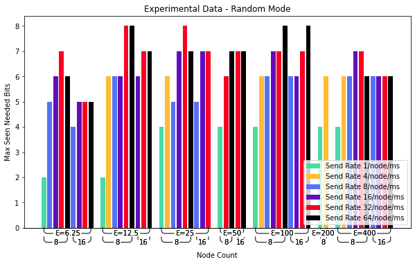
Figure 4. Value of u for wait-free viability (Random Network)

5.1.4. Effect of network topology.

We note that the results for the leader network mode and hub and spoke network mode are similar with subtle differences. Specifically, in the leader network mode, the actual clock skew is higher as one node consistently is ahead of others. This causes a higher baseline as well as larger variation. The same effect is observed in hub and spoke network where the hub node sees all the messages from the spoke nodes. For the hub and spoke network, we also observe that the value of u is more sensitive to $\epsilon$ especially at low values. For both these networks, we observe higher variability in the number of needed bits resulting in certain anomalies such as those where increasing the value of $\epsilon$ causes the value of u to reduce.

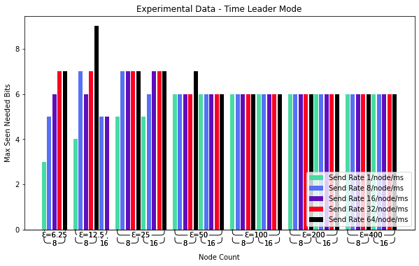
Figure 5. Value of u for wait-free viability (Time Leader Network)

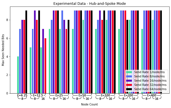
Figure 6. Value of u for wait-free viability (Hub-and-Spoke Network)

5.1.5. Causes of anomalies in simulation results.

We note that we do see some exceptions to the above observations. We note that these are due to the long tail of a probabilistic distribution where a very small number of events need a larger number of bits. As an illustration, we consider the result for $\epsilon=6.25$ms, $N=8$, $S=64$. where $\sim\!736$M events were created.

Of these, $\sim\!731$M events needed 0 bits, $\sim\!2$M events needed 1 bit. Only 142 events needed 9 bits (the maximum observed for this simulation). In other words, less than 1 in 1 million events needed all 9 bits. Since the probability of occurrence of such events is very low, we do see some instances where even with a small value of $\epsilon$, the number of bits required is high.

We see that this effect is higher in hub-and-spoke network; this is partly due to the fact that if the hub node generates an event that needs a higher number of bits then it has a substantial potential to affect multiple spoke nodes. In addition, the hub node will see events generated by every other node, and thus has a higher than normal potential to see high-lpt events. The raw data for the number of events and bits required is available at (Appleton2020PWCData, ).

5.1.6. Delays due to insufficient extraneous bits.

The above analysis also shows that if the number of available bits is low and we choose to delay certain messages (as done in Algorithm 2) then the number of affected messages is very small. For example, in the analysis from the previous paragraph, even though 9 bits are required for wait-free operation, if we had used only 4 (respectively 6) bits then 0.033% (respectively 0.01%) of messages would be delayed.

5.2. Experimental Analysis

In addition to the above, we performed a version of this experiment on physical hardware. This allows less control over the environment, but produces about 100 times the number of events in a similar time span.

The experiment was performed using seven hosts on a local network, whose send rates varied from $\sim\!19,000$ messages sent per second to $\sim\!126,000$ at the other extreme. The average send rate across the system was $\sim\!43,000$ messages per second. Traffic was generated randomly, as in the simulation’s random mode, except that it was not rate limited. Messages were sent as fast as the hardware allowed while maintaining consistent locking on the $pwc$ object.

Figure 7. Probability of needing a given number of bits to represent a timestamp without delay

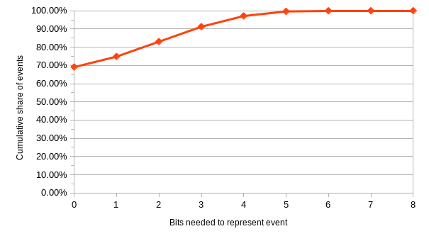
Figure 8. Given number of bits, what portion of events can be represented by a timestamp without delay

Overall, the experiment had results very similar to the simulations. About 1 in 25,000 events required more than 6 extraneous bits, and about 1 in 770,000 required more than 7. All events of the $\sim\!103$ billion could be represented with 8 extraneous bits. From this, we find that the number of bits needed is 8 or less (which corresponds to applications requiring resolution of 60 $ns$).

One feature of Figure 7 which may seem unusual at first glance is that the number of events with an lpt bit width of 1 is smaller than of sizes 0 and 2. This makes sense, however, when one considers the number of values covered by that range. Bit width 0 can only represent the value 0, so all timestamps with a freshly generated hpt will generate this. As seen in Figure 9, events with $\textsf{lpt}=0$ are very common. Moving to a bit width of 1 only allows you to represent one additional value. So while values in bit widths 2, 3, and 4 are less common, this is overcome by the fact that they add a larger range of possible values.

As above, all data and source code may be found at (Appleton2020PWCData, ).

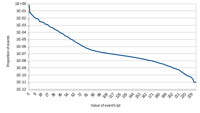
Figure 9. Proportion of events with a given lpt value

6. Discussion

In this section, we discuss some of the questions raised by PWC. A few additional questions are discussed in Appendix.

6.1. Comparison of HLC and PWC

There are some subtle differences between the clocks presented in this paper and those in (KDMA2014OPODIS.HLC, ). HLC maintains two parts: $l$ and $c$, where $l$ value is close to the physical clock and $c$ is a counter. To make it backward compatible with the physical clock, the extra information associated with HLC is saved in the lower bits of the physical clock. The most significant bits of the HLC timestamp for event $e$ on process $j$ correspond to the physical time of $j$ when event $e$ occurred. By contrast, from Lemma 3.4, the most significant bits of PWC timestamp for event $e$ on process $j$ corresponds to the physical time of some process $k$ in the system.

6.2. Disadvantages of PWC

These subtle differences have several implications: For one, the most significant bits of HLC of event $e$ on process $j$ match with the physical clock of $j$. This means that if HLC is used to compare time on the same process then the difference in HLC value is expected to be close to that in the physical clock. On the other hand, in PWC, the most significant bits correspond to the physical clock of some process but not necessarily process $j$. This means that if we compare two pwc values on the same process then their difference may be affected by $\epsilon$.

6.3. Advantages of PWC over HLC

The above benefits of HLC come at a cost that makes PWC attractive in many scenarios. For example, in HLC, the difference between the $l$ value and the $pt$ value can be as large as $\epsilon$, the clock skew. Thus, if the clock skew is $10ms$ then the bits allocated to $l-pt$ must be large enough to represent a skew of $1ms$. If clock granularity is $10\mu s$ then it implies that $l-pt$ may have 1000 possible values thereby requiring 10 bits. If the clock granularity is $0.1\mu s$ and clock skew is $10ms$ then $l-pt$ would require 17 bits. This is a severe limitation for HLC. (Plus, bits required for $c$ are extra.) In PWC, however, the value of $l-pt$ is not stored in the lower bits of the physical clock. For example, if the clock skew is $10ms$ and each process sends 1000 messages per second then (based on the analysis in Section 3.2), having just 4 extraneous bits is sufficient. Thus, PWC is useful in many scenarios where HLC is not.

HLC timestamp puts limits under which HLC can be used. In particular, if 16 bits are no longer available, it implies that the application must not generate two events within $15\ \mu s$. As $\delta_{se}$ and $\delta_{re}$ could be as small as $1\ \mu s$, this resolution is not sufficient if an application needs to send several messages as fast as possible in a short period of time (micro-burst). By contrast, PWC can be used even in scenarios where an application needs clock resolution of $10-100ns$.

Additionally, PWC is more resilient to clock skew errors. If clock skew errors increase, it may not be possible to save $l-pt$ (whose value can be as large as the clock skew) in the assigned space. By contrast, PWC is not affected by transient clock skew errors. As discussed in Section 5, even a clock synchronization error of $400ms$ does not significantly affect the number of extraneous bits required.

Another, possibly more important benefit of PWC is that the comparison of clocks is just an integer comparison. It does not require decoding the timestamp necessary for HLC. If we just use integer comparison then the comparison of HLC timestamp can provide incorrect information.

6.4. HLC Limitation for Comparison of Timestamps

In this section, we discuss the claim that HLC timestamps cannot be compared with standard $<$ operation to deduce causal information. To illustrate this, consider two timestamps $e$ and $f$ with HLC timestamps shown in Figure 10. Observe that with these timestamps $l.e=15,c.e=0$ and $l.f=14+5=19,c.f=0$. However, if we compare these timestamps as integer timestamps then we would conclude that $HLC.e$ is larger than $HLC.f$. In other words, without suitable encoding/decoding, a comparison of HLC timestamps would lead to incorrect conclusions. By contrast, PWC does not have this issue. In other words, backward compatibility of PWC is superior to that of HLC.

Figure 10. Example of HLC timestamps of events $e$ (top) and $f$ (bottom). By HLC format, the timestamp of $e$ is smaller than $f$. However, if the timestamps are treated as 64-bit integers, the value for $e$ is larger than the value for $f$. (Leading zeros are omitted)

6.5. Dealing with an Unknown Value of $\epsilon$

Algorithm 1 did not use $\epsilon$. Hence, the algorithm can be used even if $\epsilon$ is not known or is highly variable. Value of $\epsilon$ is needed only to determine if Algorithm 1 is viable. Furthermore, the changes in Algorithm 2 can be used to ensure that the algorithm remains viable by adding occasional small delays on messages. Thus, PWC can be easily used in scenarios where the exact value of $\epsilon$ is not known.

6.6. Dealing with Dynamic Value of u

The value of u can also be changed dynamically. The easiest way to do this is to communicate to all processes that the value of u should be changed to $\textsf{u}^{\prime}$ at PWC time $t^{\prime}$, where $t^{\prime}$ is sufficiently larger. Furthermore, it is also possible that u can be changed independently. For example, consider the case where process $j$ assumes $\textsf{u}=4$ and process $k$ assumes $\textsf{u}=5$. In this case, if Algorithm 1 remains viable under the assumption that $\textsf{u}=4$ then it would be correct under the scenario where process $j$ treats $\textsf{u}=4$ and process $k$ treats $\textsf{u}=5$. Due to reasons of space, we omit the proof of this claim

6.7. Dealing with Non-Monotonic Clocks

While a monotonic clock is ideal for running PWC, it can handle a transient clock drift due to (for example) a negative leap second. First, we observe that this type of underlying clock drift does not affect causality, i.e., even in the presence of a negative leap second, Theorem 3.3 remains valid. It can only affect the condition related to the overflow of the clock. Specifically, if a clock can go backward, the number of events that may be created for a given hpt value increases. In turn, the number of bits required to prevent overflow may increase. Furthermore, the approach used in Algorithm 2 will handle potential overflows by delaying events when needed.

6.8. Use of PWC in Evaluating Elapsed Time

One use of physical clocks is in evaluating time elapsed between two events. Specifically, if $pt.e$ and $pt.f$ denote the physical clock of event $e$ and $f$, we can use $pt.f-pt.e$ to determine the time elapsed between $e$ and $f$.

Both HLC and PWC can be used as a substitute. Errors due to the use of HLC or PWC are comparable in nature. In HLC, the $l$ value can differ from $pt$ by $\epsilon$ (with $l$ value always higher or equal). Hence, while comparing $l.f-l.e$, there is a potential error of $2\epsilon$ when compared with $pt.f-pt.e$. A similar error can occur with PWC.

6.9. Use of PWC as Logical Clock

Based on Theorem 3.3, we see that pwc can be used in any place where logical clock can be used. For example, it can be used in mutual exclusion algorithms such as Lamport’s algorithm (Ghosh14, ).

6.10. Use of PWC as Physical Clock

PWC can also be used as a replacement for physical clocks. Specifically, algorithms such as Spanner rely on physical clocks (synchronized within some bound $\epsilon$). Based on Theorem 3, PWC can be used in its place. Furthermore, with PWC, some of the deficiencies (e.g., commit-wait delay) are removed without adding any overhead. Likewise, PWC can also be used in algorithms such as CausalSpartan (CausalSpartan.RDK17SRDS, ) to obtain causal consistency without introducing delays caused by clock skew. As discussed above, HLC can also be used to remove some of the disadvantages discussed above. However, a key advantage of PWC over HLC is that PWC can be used even when clock skew is high. In this case, HLC is limited as bits are needed to save the $l-pt$ value. By contrast, PWC can be used even with large clock skews as it does not explicitly store values such as $l-pt$.

7. Related Work

Recording timestamps of events is critical for reconstructing and debugging the execution of a distributed program. The natural solution to record timestamps of events is the physical time which is the reading of the local clock of the machine on which the process runs. However, physical clocks are not perfectly synchronized, which makes it possible that $pt.e>pt.f$ but $e$ actually occurred after $f$ or vice versa, i.e. $e$ actually occurred after $f$ but $pt.e>pt.f$.

TrueTime (CDEFFFGGHH13TOCS, ) is another physical-clock-based approach but it requires dedicated hardware as well as delayed operation if needed to clear the uncertainty. Lamport’s logical clock (Lamport78CACM, ) guarantees that if event $f$ causally depends on event $e$ then the logical clock of $f$ is strictly greater than $e$. However, the converse of this property is not true, i.e. one could not infer the causality between two events based on their logical timestamps. In (fetzer, ), authors use partially synchronized clocks to implement several protocols in distributed systems. The concept of encoding low-end bits to provide reliable ordered delivery is considered in (sscmp, ). The two-way causality property is provided by vector clocks (Mattern89PDA, ; Fidge87, ), dependence blocks (SM94DC, ) which keep track of and combine causality information on all processes. However, the size of vector clocks is $O(n)$ where $n$ is the number of processes, which is prohibitively expensive for large distributed systems. To handle the dynamic nature of distributed systems and reduce the space complexity of vector clocks, interval tree clocks (ABF2008OPODIS.intervaltreeclock, ) and Bloom clocks (ramabaja2019arxiv.bloomclock, ) are proposed.

Both logical and vector clocks are timestamps that completely independent from the physical clock. Some works combine the information of logical and physical clock to improve the causality decision as well as reduce the size of the timestamp (KDMA2014OPODIS.HLC, ; DK13LADIS, ; VK2018SIROCCO, ). Among those, Hybrid Logical Clock (KDMA2014OPODIS.HLC, ) is the work closest to the $pwc$ described in this paper. In HLC, the bit array storing the timestamp is separated into two parts: one for physical clock information and the other for logical clock information (causality). Thus, manipulation of HLC requires encoding and decoding the bit array. By contrast, in $pwc$, the whole bit array is treated as a single integer and there is no need for encoding/decoding the causality information.

8. Conclusion

In this paper, we presented PWC that was a physical clock that also provided information to deduce one-way causality. We achieved this by observing that a certain number of extraneous/redundant bits are available in a physical clock. We used these bits to provide causal information.

PWC provides several benefits over HLC (KDMA2014OPODIS.HLC, ). For one, PWC is applicable in many systems where clock skew is larger or more variable. HLC is limited by the fact that it needs to store the value of $l-pt$ and this value depends upon $\epsilon$, the clock skew. By contrast, PWC is unaffected by transient errors that cause significantly higher clock skew. Second, PWC works correctly even if the number of extraneous bits is small; we find that even 9 bits (time resolution of 120 $\ ns$) are sufficient for PWC. By contrast, HLC generally requires a larger number of bits (16 proposed in (KDMA2014OPODIS.HLC, ) which corresponds to clock resolution of $15\mu s$). Hence, HLC is not able to handle microbursts of messages that PWC can handle. Thus, PWC is more applicable than HLC. Third, the backward compatibility of PWC with physical clocks is better than that of HLC. Specifically, to get the HLC comparison right to deduce (one-way) causality, we need to decode the timestamps. With PWC, just integer comparison suffices.

A key disadvantage of PWC over HLC (KDMA2014OPODIS.HLC, ) is that the most significant bits of $\textsf{pwc}.{e_{j}}$ correspond to the physical clock of some process $k$. By contrast, the most significant bits of $hlc.{e_{j}}$ correspond to the physical clock of $j$.

HLC and PWC provide several common features. Both are strictly increasing. Both can be used in place of logical or physical clock. Both can be used to eliminate delays caused by clock skew in applications such as Spanner (CDEFFFGGHH13TOCS, ), CausalSpartan (CausalSpartan.RDK17SRDS, ).

There are several opportunities provided by PWC that would permit additional future extensions of PWC. For example, PWC also provides a possibility of obtaining (two-way) causality with physical clocks. Specifically, if the available extraneous bits exceed the number of bits needed to prevent overflow, additional bits could be used to provide additional information that could be used to deduce when two events are concurrent.

Appendix A Appendices

A.1. HLC Algorithm

Here, we provide the algorithm for HLC from (KDMA2014OPODIS.HLC, ).

1:

2:$l$’$.i:=l.i$

3:$l.i:=max(l$’$.i,pt.i)$ //tracking maximum time event, $pt.i$ is physical time at process $i$

4:If ($l.i=l$’$.i$) then $c.i:=c.i+1$ //tracking causality

5:Else $c.i:=0$

6:Timestamp the event (and the message for send event) with $l.i$, $c.i$

7:

8:$l$’$.i:=l.i$

9:$l.i:=max(l$’$.i,l.m,pt.i)$ // $l.m$ is $l$ value in the timestamp of the message received

10:If ($l.i=l$’$.i=l.m$) then $c.i:=max(c.i,c.m)+1$

11:Elseif ($l.i=l$’$.i$) then $c.i:=c.i+1$

12:Elseif ($l.i=l.m$) then $c.i:=c.m+1$

13:Else $c.i:=0$

14:Timestamp event with $l.i$,$c.i$

Algorithm 3 Hybrid Logical Clocks (HLC) Algorithm from (KDMA2014OPODIS.HLC, )

A.2. Omitted Proofs

A.2.1. Proof of Observation 3.2

This follows by induction and Observation 3.2. Specifically, if $f$ is the a send event and $e$ is the previous event before $f$ then by Observation 3.2, $\textsf{pwc}.j+1\leq\textsf{clpt}.j$. It follows that for event $f$, $\textsf{pwc}.f$ would be set to be equal to $\textsf{clpt}.j$. And, by definition of lpt, $\textsf{lpt}.f$ would be $0$. $\square$

A.2.2. Proof of Lemma 3.2

We consider two cases: Event $f$ is a local/send event (on process $j$) or it is a receive event (on process $j$). For the first, case, note that, by definition, the least significant bits of clpt.j are 0. If the value of $\textsf{lpt}.j$ is set to $v,v>0$, it must be due to the fact that $\textsf{pwc}.f$ was set to $\textsf{pwc}.j+1$, where $\textsf{pwc}.j$ corresponded to the timestamp of the previous event on $j$. Thus, the above statement is satisfied by letting $e$ be the previous event on $j$. If $f$ is a receive event then a similar argument follows except that $e$ would be either the previous event on $j$ or the message send event. $\square$

A.2.3. Proof of Lemma 3.4

​
The first part is trivially true.

For the second part, we can prove this by induction on the created events. The base case (initial events) is trivially satisfied. Next, let $e$ and $f$ be two consecutive events on process $j$. First, we consider the case where $f$ is a send event. By induction, we assume that $\textsf{pwc}.e\leq\textsf{clpt}.k_{e}+2^{\textsf{u}}$, where $\textsf{clpt}.k_{e}$ was the value of $\textsf{clpt}.k$ when $e$ was created. Let $\textsf{clpt}.k_{f}$ be the value of $\textsf{clpt}.k$ when $f$ was created. Clearly, $\textsf{clpt}.k_{e}\leq\textsf{clpt}.k_{f}$. We consider two cases

• $\textsf{pwc}.f$ is set to $\textsf{pwc}.e+1$. By induction, there exists $k$ such that $\textsf{pwc}.e\leq\textsf{clpt}.k_{e}+2^{\textsf{u}}$. Since $\textsf{clpt}.k_{e}\leq\textsf{clpt}.k_{f}$, we have $\textsf{pwc}.e\leq\textsf{clpt}.k_{f}+2^{\textsf{u}}$. Furthermore, if $\textsf{pwc}.e=\textsf{clpt}.k_{f}+2^{\textsf{u}}$ then creation of event $f$ would imply that Algorithm 1 has an overflow. Hence, $\textsf{pwc}.e<\textsf{clpt}.k_{f}+2^{\textsf{u}}$. Thus, $\textsf{pwc}.e+1\leq\textsf{clpt}.k_{f}+2^{\textsf{u}}$. In other words, $\textsf{pwc}.f\leq\textsf{clpt}.k_{f}+2^{\textsf{u}}$.

• $\textsf{pwc}.f$ is set to $\textsf{clpt}.j$. Then, the statement is trivially true if we let $k=j$.

If $f$ is a receive event, the proof is similar except that we need to consider three cases for setting $\textsf{pwc}.f$. $\square$

A.2.4. Proof of Theorem 3

Proof. Without loss of generality, let $\textsf{pwc}.j<\textsf{pwc}.k$. Then, we have

	$\textsf{pwc}.k-\textsf{pwc}.j$
$\leq$	$\textsf{pwc}.k-\textsf{clpt}.j$	// $\textsf{pwc}.j\geq\textsf{clpt}.j$
$\leq$	$\textsf{clpt}.k+2^{\textsf{u}}-\textsf{clpt}.j$	// Lemma 3.4
$\leq$	$pt.k+2^{\textsf{u}}-\textsf{clpt}.j$	// $pt.k>\textsf{clpt}.k$
$\leq$	$pt.k+2^{\textsf{u}}-(pt.j-2^{\textsf{u}})$	// $\textsf{clpt}.j>pt.j-2^{\textsf{u}}$
$\leq$	$\epsilon+2*2^{\textsf{u}}=\epsilon+2^{\textsf{u}+1}$

A.3. Experimental measurement of $\delta_{se},\delta_{re}$

We set up a cluster of machines connected via a switch in a local network. The switch capacity is 10 Gbps. Each machine is equipped with a 1000 Mbps network card. To measure the time to send a message $\delta_{send}$ (moving the message from the process to the network interface card), we have one machine send messages to 5 machines as fast as possible in 200 seconds. The value of $\delta_{send}$ is approximately calculated as the total time (200 seconds) divided by the number of messages sent by the sending machine. To measure $\delta_{receive}$ (moving the message from the network interface card to the receiving process), we have 5 machines sending messages to one machine in 200 seconds. The value of $\delta_{receive}$ is approximately calculated as the total time divided by the number of messages received at the receiving machine. All messages are sent via User Datagram Protocol. The message size is varied between 1 byte and 1,400 bytes.

From our experiments, we observe that the time to send or receive a message is a linear function of the message size. In particular:

$$\delta_{send},\delta_{receive}=const_{1}+const_{2}\times message\_size$$

Where $const_{1}$ (unit is nanosecond) is the time to move the message through the protocol stack, $const_{2}$ (unit is nanosecond/byte) is the time it takes the network adapter to transmit (or receive, respectively) one byte of data to (or from, respectively) the cable.

The values of $const_{1}$ and $const_{2}$ depend on the machine and whether it is a receiver or a sender. In our measurement:

• $const_{1}$ is a few microseconds. Specifically, it varies from 1,162 to 2,379 nanoseconds for senders and varies from 1,269 to 4,137 nanoseconds for receivers.

• $const_{2}$ varies from 6.6 to 7.6 nanosecond/byte for senders and varies from 6.1 to 15.5 nanosecond/byte for receivers. The advertised speed of network adapter on the machines in our lab is 1,000 Mbps (8 nanoseconds/byte).

With message payload between 1 byte and 1,400 bytes (to fit in an Ethernet frame), the time to send a message $\delta_{send}$ is between $1-12$ microseconds, and the time to receive a message $\delta_{receive}$ is between $1-24$ microseconds.

References

- (1) D. L. Mills, “Network time protocol (ntp),” Internet Requests for Comments, RFC Editor, RFC 958, September 1985.
- (2) L. Lamport, “A new solution of dijkstra’s concurrent programming problem,” Communications of the ACM, vol. 17, no. 8, pp. 453–455, 1974.
- (3) J. C. Corbett, J. Dean, M. Epstein, A. Fikes, C. Frost, J. J. Furman, S. Ghemawat, A. Gubarev, C. Heiser, P. Hochschild et al., “Spanner: Google’s globally distributed database,” ACM Transactions on Computer Systems (TOCS), vol. 31, no. 3, p. 8, 2013.
- (4) J. Du, C. Iorgulescu, A. Roy, and W. Zwaenepoel, “Gentlerain: Cheap and scalable causal consistency with physical clocks,” in Proceedings of the ACM Symposium on Cloud Computing, ser. SOCC ’14. New York, NY, USA: ACM, 2014, pp. 4:1–4:13.
- (5) M. Roohitavaf, M. Demirbas, and S. S. Kulkarni, “Causalspartan: Causal consistency for distributed data stores using hybrid logical clocks,” in 36th IEEE Symposium on Reliable Distributed Systems, SRDS 2017, Hongkong, China, September 26 - 29, 2017, 2017, pp. 184–193.
- (6) A. Charapko, A. Ailijiang, M. Demirbas, and S. Kulkarni, “Retrospective lightweight distributed snapshots using loosely synchronized clocks,” in Distributed Computing Systems (ICDCS), 2017 IEEE 37th International Conference on. IEEE, 2017, pp. 2061–2066.
- (7) S. S. Kulkarni, M. Demirbas, D. Madappa, B. Avva, and M. Leone, “Logical physical clocks,” in International Conference on Principles of Distributed Systems. Springer, 2014, pp. 17–32.
- (8) D. Mills, J. Martin, J. Burbank, and W. Kasch, “Network time protocol version 4: Protocol and algorithms specification,” Internet Requests for Comments, RFC Editor, RFC 5905, June 2010.
- (9) “Ieee standard for a precision clock synchronization protocol for networked measurement and control systems,” IEEE Std 1588-2008 (Revision of IEEE Std 1588-2002), pp. 1–300, 2008.
- (10) L. Lamport, “Time, clocks, and the ordering of events in a distributed system,” Commun. ACM, vol. 21, no. 7, pp. 558–565, Jul. 1978.
- (11) A. Arora and M. G. Gouda, “Distributed reset,” IEEE Trans. Computers, vol. 43, no. 9, pp. 1026–1038, 1994.
- (12) “Experimental data and source code for the paper ”Achieving Causality with Physical Clocks”,” https://gist.github.com/AnonymousPaperPWC/39001b43cda3b5aa3a99783b0b418c74, 2021.
- (13) S. Ghosh, Distributed systems: an algorithmic approach. CRC press, 2014.
- (14) C. Fetzer and M. Raynal, “Elastic vector time,” in 23rd International Conference on Distributed Computing Systems (ICDCS 2003), 19-22 May 2003, Providence, RI, USA. IEEE Computer Society, 2003, p. 284.
- (15) U. Schmid and A. Pusterhofer, “SSCMP: the sequenced synchronized clock message protocol,” Comput. Networks ISDN Syst., vol. 27, no. 12, pp. 1615–1632, 1995.
- (16) F. Mattern, “Virtual time and global states of distributed systems,” Parallel and Distributed Algorithms, vol. 1, no. 23, pp. 215–226, 1989.
- (17) C. J. Fidge, “Timestamps in message-passing systems that preserve the partial ordering,” in Proceedings of the 11th Australian Computer Science Conference (ACSC), K. Raymond, Ed., 1988, pp. 56–66.
- (18) R. Schwarz and F. Mattern, “Detecting causal relationships in distributed computations: In search of the holy grail,” Distributed computing, vol. 7, no. 3, pp. 149–174, 1994.
- (19) P. S. Almeida, C. Baquero, and V. Fonte, “Interval tree clocks,” in Principles of Distributed Systems, 12th International Conference, OPODIS 2008, Luxor, Egypt, December 15-18, 2008. Proceedings, ser. Lecture Notes in Computer Science, T. P. Baker, A. Bui, and S. Tixeuil, Eds., vol. 5401. Springer, 2008, pp. 259–274.
- (20) L. Ramabaja, “The bloom clock,” arXiv preprint arXiv:1905.13064, 2019.
- (21) M. Demirbas and S. Kulkarni, “Beyond truetime: Using augmentedtime for improving google spanner,” in Workshop on Large-Scale Distributed Systems and Middleware (LADIS), 2013.
- (22) V. T. Valapil and S. S. Kulkarni, “Biased clocks: A novel approach to improve the ability to perform predicate detection with O(1) clocks,” in Structural Information and Communication Complexity - 25th International Colloquium, SIROCCO 2018, Ma’ale HaHamisha, Israel, June 18-21, 2018, Revised Selected Papers, 2018, pp. 345–360.