Climate Modelling in Low-Precision: Effects of both Deterministic & Stochastic Rounding.

Abstract

Motivated by recent advances in operational weather forecasting, we study the efficacy of low-precision arithmetic for climate simulations. We develop a framework to measure rounding error in a climate model which provides a stress-test for a low-precision version of the model, and we apply our method to a variety of models including the Lorenz system; a shallow water approximation for turbulent flow over a ridge; and a coarse resolution global atmospheric model with simplified parameterisations (SPEEDY). Although double precision (52 significant bits) is standard across operational climate models, in our experiments we find that single precision (23 sbits) is more than enough and that as low as half-precision (10 sbits) is often sufficient. For example, SPEEDY can be run with 12 sbits across the entire code with negligible rounding error and this can be lowered to 10 sbits if very minor errors are accepted, amounting to less than 0.1 mm/6hr for the average grid-point precipitation, for example. Our test is based on the Wasserstein metric and this provides stringent non-parametric bounds on rounding error accounting for annual means as well as extreme weather events. In addition, by testing models using both round-to-nearest (RN) and stochastic rounding (SR) we find that SR can mitigate rounding error in both turbulent regimes and slow processes such as heat diffusion in a land-surface component, where low-precision is notably problematic with RN due to stagnation. Thus our results also provide evidence that SR could be relevant to next-generation climate models. While many studies have shown that low-precision arithmetic can be suitable on short-term weather forecasting timescales, our results give the first evidence that a similar low precision level can be suitable for climate. I.e. In our applications, we find that small rounding errors in the short-term forecast do not accumulate in time so as to disrupt the long-time statistics of the system.

1 Introduction

Modern numerical earth system models require enormous amounts of computational resources and place significant demand on the world’s most powerful supercomputers. As such, operational forecasting centres are stretched to make best use of resources and seek ways of reducing unnecessary computation and memory allocation for the sake of performance wherever possible.

One idea to improve computational efficiency which has gained attention in recent years is to utilize low-precision arithmetic—in place of conventional 64 bit arithmetic—for computationally intensive parts of the code. This has been accompanied by parallel trends in deep learning where low precision is deployed routinely and for which novel hardware is now emerging [11, 19]. Whether such hardware can be exploited for weather & climate, however, ultimately depends on the cumulative effect of rounding error. In fact, a number of studies have shown that much numerical weather prediction, at least on the short timescales relevant for forecasts, can be optimized for low precision [2, 13, 14, 15, 23] and forecasting centres are already exploiting this in operations. The European Centre for Medium-Range Weather Forecasts has now ported the atmospheric component of its flagship Integrated Forecast System to single precision [18, 25] while MeteoSwiss and the UK Met Office have tested single and mixed-precision codes respectively [10, 22].

As operational weather forcasters experiment with more efficient low-precision hardware, it is natural to ask whether low precision is suitable for climate modelling (i.e. long time-scales) and this is the question addressed by the current paper. Compared to weather forcasting, where research in low precision has focused to date, climate modelling presents a different problem requiring some new techniques. While an ensemble weather forecast seeks a relatively localized probability distribution over the possible states of the atmosphere at a given time, the exact state is understood to be totally unpredictable on long timescales due to chaos, and a climate model seeks instead to approximate the statistics of states over a long time period (in the language of ergodic theory, the climatological object of interest is the invariant probability distribution). Thus the test for a low-precision climate model should be whether it has the same statistics (invariant distribution) as its high-precision counterpart.

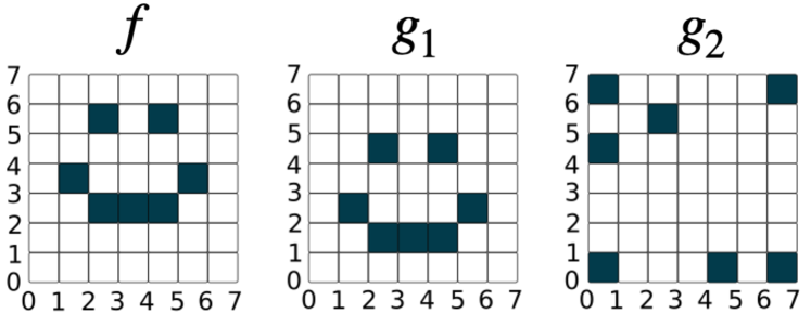
Figure 1: An example of the Wasserstein distance (WD). The WD from $g_{1}$ to $f$ is 1, where an optimal transport strategy is to shift all of the probability mass up by one unit. By contrast, it is easily seen that $\text{WD}(f,g_{2})>1$, reflecting the intuition that $g_{1}$ is a better approximation of $f$ than is $g_{2}$. Figure motivated by [21].

We develop such a test based on the Wasserstein distance (WD) from optimal transport theory which provides a natural notion of closeness between probability distributions. The WD is defined as the cost of an optimal strategy for transporting probability mass between two distributions with respect to a cost $c(x,y)$ of transporting unit mass from $x\in\mathbb{R}^{d}$ to $y\in\mathbb{R}^{d}$, where throughout this paper we take $c(x,y)=|x-y|$ so that cost has the same units as the underlying field.

The WD is an appropriate metric for this study because: (1) it is non-parametric; (2) it has favourable geometrical properties (cf. Fig. 1); (3) it is interpretable in appropriate physical units; and (4) it bounds a range of expected values covering both the mean response and extreme weather events. The metric is popular in machine learning [1] and has recently been suggested as an appropriate measure of skill in climate modelling [21, 27, 28], however since it is not so well-known within the community, a survey of the WD including a rigorous definition and discussion of computational techniques are given in App. A. In particular, the reader is encouraged to see A.1 for further discussion of (1)-(4).

Any test can only bound the effects of rounding error at low precision relative to the variability of probability distributions generated by a corresponding high-precision experiment. Experiments must thus be carefully designed to minimise such variability in order to isolate the effects of rounding error. For example, by taking an ensemble of sufficiently long integrations one can reduce initial-condition variability, and by keeping external factors such as greenhouse gas emmisions annually-periodic one can reduce variability due to non-stationarity. A choice of metric with strong properties (e.g. (1)-(4)) is then crucial for interpretation of the resulting bounds on rounding error in order to have confidence in the reliability of a low-precision model. Although we developed our methods to measure rounding error, we hope they might also be of interest to the broader climate modelling community.

2 The Lorenz system

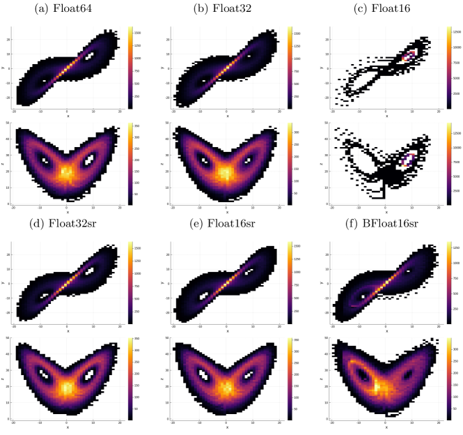
Figure 2: The Lorenz system integrated and data-binned at different precisions

To illustrate our methods which will later be applied to more complex climate models, we first consider the Lorenz system

$$\begin{split}\frac{dx}{dt}&=10\left(y-x\right)\\ \frac{dy}{dt}&=\big{(}\nicefrac{{8}}{{3}}-z\big{)}x-y\\ \frac{dz}{dt}&=xy-28z.\end{split}$$ (1)

Derived first by Lorenz [17] in a study of convection, (1) exhibits features of nonlinear dynamics representative of the real atmosphere [20]. The system has a fractal attractor $\mathcal{A}\subseteq\mathbb{R}^{3}$ and the dynamics on $\mathcal{A}$ is chaotic, rendering the precise numerical approximation of any specific orbit futile. On the other hand, a study of asymptotics on $\mathcal{A}$ reveals statistics common across orbits which one may hope to approximate. Indeed, there exists a unique invariant probability distribution $\nu$ supported on $\mathcal{A}$ such that for almost any orbit $\mathbf{x}(t)=(x(t),y(t),z(t))$ initiated in the basin of attraction of $\mathcal{A}$ and any bounded continuous $\phi$

$$\lim_{T\uparrow\infty}\left\{\frac{1}{T}\int_{0}^{T}\phi(\mathbf{x}(t))dt\right\}=\iiint\phi(\mathbf{x})d\nu(\mathbf{x})$$ (2)

cf. [24]. Thus $\nu$ encodes the long-time statistics of the system. For example, taking $\phi(\mathbf{x})=1$ for $\mathbf{x}\in B$ and $\phi(\mathbf{x})=0$ outside of a neighbourhood of $B$, from (2) we see the average time an orbit spends in a region $B$ is the probability mass $\nu(B)$. In the context of climate modelling, the test for a low-precision integration of (1) is whether it produces approximately the same $\nu$ as its high-precision counterpart.

We first sampled 10 initial conditions $i_{0},\ldots,i_{9}\in\mathbb{R}^{3}$ from a normal distribution with unit variance centred at the centre of mass of the attractor $\mathcal{A}$. We then integrated (1) at high-precision (Float64) initialised at initial conditions $i_{0},\ldots,i_{4}$ for $220\hskip 2.0pt000$ model time units (mtu) each and discarded the first $20\hskip 2.0pt000$ mtu as spin-up to allow for any orbits initially perturbed off $\mathcal{A}$ to return to $\mathcal{A}$, and we labelled these five runs as the control ensemble $e^{\mathrm{control}}_{i}$. Next, for each comparison arithmetic—including Float64—we integrated (1) initialised at initial conditions $i_{5},\ldots,i_{9}$ for $220\hskip 2.0pt000$ mtu, discarded the first $20\hskip 2.0pt000$ mtu and labelled these as the competitor $e_{j}$. Each integration used the Runge-Kutta 4th order scheme with a time step of $dt=0.002$. For background on the different arithmetic formats and stochastic rounding, see App. B.

In general, results will be sensitive both to the choice of numerical scheme and the time-step, however we won’t dwell on such issues since our aim is to develop a method to measure rounding error in a climatological context, rather than to obtain an optimal integration.

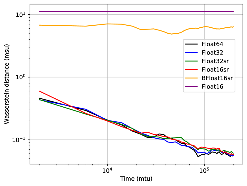
Figure 3: Measuring rounding error in the climate of the Lorenz system. Plot shows Wasserstein distances between the probability distributions generated by low-precision and high-precision ensembles (binwidth 6.0) where black is high precision vs high precision for reference.

Integrations are binned and plotted in Fig. 2. Whilst the Float32, Float32sr, and Float16sr integrations appear to approximate the high-precision attractor well, Float16 suffers from the small number of available states forcing the evolution into an early periodic orbit while we found BFloat16 collapsed on a point attractor with this fine time-step, though both of these integrations were notably improved by stochastic rounding. For each arithmetic we computed the ensemble mean Wasserstein distance (WD, cf. App. A) between the 5 probability distributions generated by $e_{i}$ and the 5 distributions generated by $e^{\mathrm{control}}_{j}$ and the evolution of this quantity with time is plotted in Fig. 3 with a log-log scale. Note that the Float64 competitor (black in Fig. 3) shows the mean WD between a pair of high precision integrations initiated at different initial conditions, and thus gives a measure of the variability of the experiment at high precision which is important to be able to draw conclusions. Fig. 3 confirms quantitatively what is suggested by Fig. 2 in that the Float32, Float32sr and Float16sr curves closely follow Float64 in the approach to statistical equilibrium, showing that rounding error is small relative to high-precision variability, whilst for BFloat16sr rounding error has notably perturbed the dynamics. The size of the high-precision variability after 100 000 mtu (cf. Fig. 3) is less than 0.1 model space units (msu) which is small in the context of distributions supported on the Lorenz attractor, which has characteristic length scale of approximately 50 msu (cf. Fig. 2).

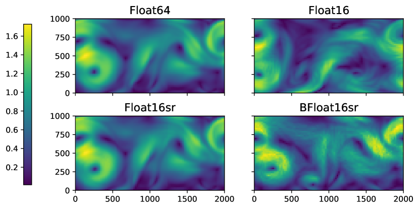
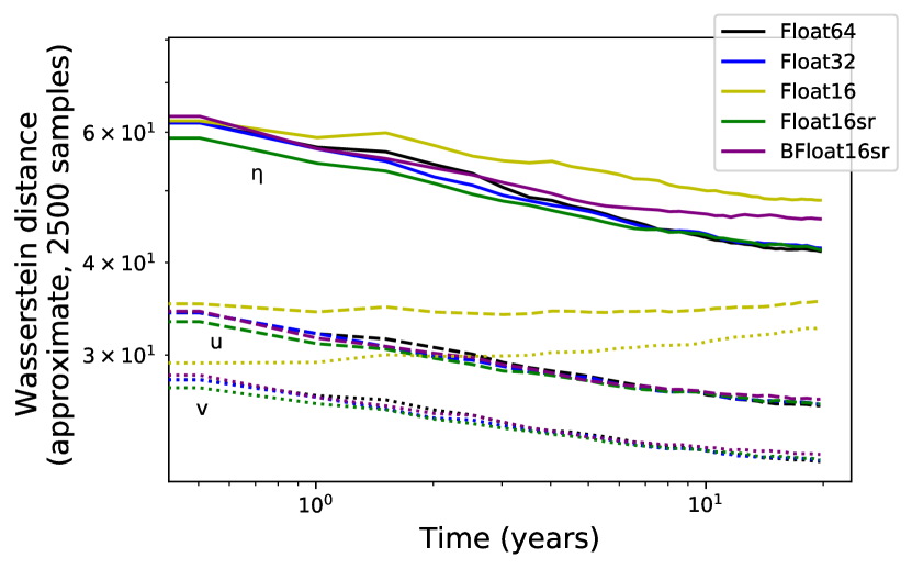
Figure 4: The shallow water model integrated at different precision levels. The left-hand plot is a snapshot of the flow speed (m/s), initiated from the same initial condition, after 50 days (a deterministic forecast) while the right-hand graph shows the effect of rounding error on climatology. Double precision variabilty in black provides a reference and errors are small relative to this variability for similarly converging distances.

To compute WDs we approximated the probability distributions by data-binning with cubed bins and a binwidth of 6 msu. This is a coarse estimation but we found results were not sensitive to decreasing bin-width (in agreement with [28]) and we also performed the same computation approximating by the empirical distributions generated by 2500 samples as well as approximating by Sinkhorn divergences, and by marginalising onto 1-dimensional distributions (cf. A.3), all of which gave analogous results.

3 A shallow water model

We next consider the shallow water model from [15] which describes turbulent flow in a rectangular ocean basin, driven by a steady zonally symmetric wind forcing over a meridionally symmetric ridge. The equations are

$$\frac{\partial\mathbf{u}}{\partial t}+(\mathbf{u}\cdot\nabla)\mathbf{u}+f\hat{\mathbf{z}}\times\mathbf{u} =-g\nabla\eta+\mathbf{D}+\mathbf{F}$$

$$\frac{\partial\eta}{\partial t}+\nabla\cdot(\mathbf{u}h) =0$$

where $\mathbf{u}=(u,v)$ is velocity, $\eta$ is surface elevation, $\mathbf{D}=-\frac{c_{D}}{h}|\mathbf{u}|\mathbf{u}-\nu\nabla^{4}\mathbf{u}$ is a nonlinear diffusive term with coefficient $\nu$ and $c_{D}$ a dimensionless parameter, $\mathbf{F}$ is wind forcing, $f$ is the Coriolis parameter, $h=H+\eta$ is layer thickness and $H$ is the time-independent depth of the water at rest describing the ridge at the fluid base. The ocean basin dimensions were taken as 2000 km by 1000 km with average depth 500 m. We integrated the equations using the scheme from [15] which uses finite differences on an Arakawa C-grid and 4th order Runge-Kutta in time combined with a semi-implicit scheme for the dissipative terms, with a time step of 6 hr, and refer to [15] for more details on the numerical scheme.

Following the methodology developed in Sec. 2 we integrated for 20 years discarding the first year of each run as spin-up, taking a 5 member ensemble for each arithmetic. Snapshots of the evolution in each case are plotted in Fig. 4a. We computed ensemble mean pairwise WDs between the distributions generated by high and low-precision ensembles and plot this quantity evolving with time in Fig. 4. We found that for Float16 and BFloat16sr rounding error is significant whilst for Float32 and Float16sr rounding error is small relative to high-precision variability. In particular, our results show that rounding errors at half-precision are successfully mitigated by stochastic rounding in this climate experiment. Again, we refer to App. B for background on these different number formats.

The main difference between the methods of this section and Sec. 2 is that we considered here a dynamical system which is high dimensional, so that approximating probability distributions is non-trivial. For Fig. 4b we approximated the invariant distributions by taking 2500 uniformly distributed random samples in time and computed WDs between the corresponding emprical distributions (cf. A.3). This approximation method does not give readily interpretable results due to a curse of dimensionality (A.3) however we obtained analagous results by marginalising onto one-dimensional subspaces. We save discussion of such marginalised results for Sec. 5 in the context of a global atmospheric model.

4 Interlude: heat diffusion in an ideal soil column.

In this section we briefly consider a very simplified land-surface component of a global climate model. This is a trivial case of climatology since all solutions converge upon a constant equilibrium temperature and so there is no need to use the WD in this setting. We include this simple example, however, because it clearly illustrates a major advantage of SR over RN—preventing stagnation.

This section was partially motivated by [12] and [6]. In [12] the authors observed that the Canadian LAnd Surface Scheme (CLASS) could not be run effectively at single-precision in large part because of an issue of stagnation. They argued that single-precision arithmetic was not appropriate for climate modelling with the scheme which relies crucially on accurate representations of slowly-varying processes such as permafrost thawing and that double precision or even quadruple precision should be adopted instead. The set-up considered here was introduced in [6] as a toy model which retained some features of CLASS, most crucially the stagnation at single-precision with RN. The authors of [6] proposed mixed precision to avoid stagnation, while the results of this section indicate that SR provides an alternative approach.

Following [6], we consider an idealised soil column which is heated from the top and thermally insulated from the bottom

$$\frac{\partial T}{\partial t}=D\frac{\partial^{2}T}{\partial z^{2}}$$

with $T(t,0)=280$, $\frac{\partial T}{\partial z}(t,H)=0$ and $T(0,z)=273$ where $T(t,z)$ is temperature in Kelvin, $H=60$ m is soil depth, and $D$=$7\times 10^{-7}\mathrm{m}^{2}\mathrm{s}^{-1}$ is the coefficient of diffusivity, and discretise as

$$T^{n+1}_{j}=T^{n}_{j}+D\Delta t\left(\frac{T^{n}_{j+1}-2T^{n}_{j}+T^{n}_{j-1}}{(\Delta z)^{2}}\right)$$ (3)

with $\Delta z=1$ m and $\Delta t=1800$ s.

We integrated for 100 years and the results are plotted in Fig. 5. Stagnation is apparent for Float32 and Float16 where the small tendancy term in (3) is repeatedly rounded down to zero, so that heat does not diffuse effectively through the soil column. This is mitigated by SR, however, which assignes a non-zero probability of rounding up after the addition in (3) (cf. Sec. B.2). Rounding error is neglegible with Float32sr and while visible as noise in Float16sr, the solution shares the large-scale pattern of Float64.

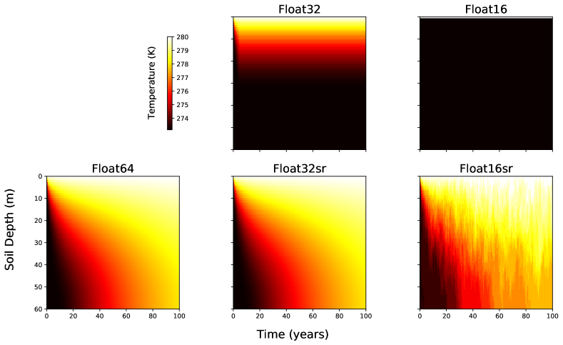
Figure 5: Heat diffusion in a soil column with different number formats and rounding modes.

To be clear, this section is not intended to imply that SR is necessary in the low-precision integration of the heat equation. There are other ways to avoid stagnation, such as increasing the time-step which is extremely small in this example and well below what is necessary for stability, or implementing a compensated summation for the timestepping. Rather, this section aims to illustrate an interesting advantage of SR in mitigating stagnation, by means of a clear and visual example. For more analysis of SR in the numerical solution of the heat equation see [3].

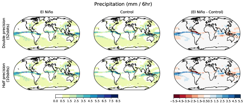
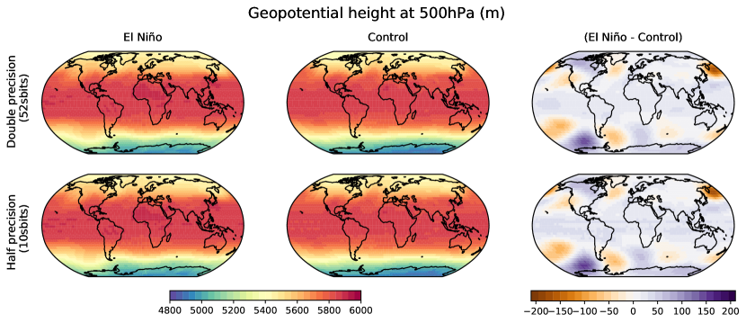
Figure 6: Annual mean response to El Niño: double vs half precision. From the perspective of the mean state, rounding error at half precision is seen to be small.

5 A global atmospheric model.

Finally, we proceed to a global atmospheric circulation model: the Simplified Parameterizations PrimitivE Equation DYnamics ver 41 (SPEEDY). SPEEDY is a coarse resolution model employing a T30 spectral truncation with a 48x96 latitude-longitude grid, 8 vertical levels and a 40 min timetep, and is forced by annually-periodic fields obtained from ERA reanalysis together with a prescribed sea surface temperature anomaly [16]. For this section, in order to isolate the effects of numerical precision we truncated only the significant bits, so that when we speak of half precision, for example, we refer to 10 significant bits (sbits) and 11 exponent bits rather than the IEEE754 5 exponent bits (i.e. overflows were not accounted for in this section).

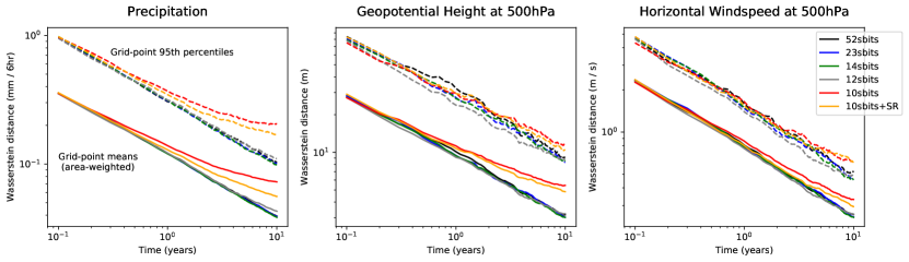
Figure 7: Measuring rounding error in SPEEDY climatology with grid point Wasserstein distances. Double precision variabilty in black provides a reference and errors are small relative to this for similarly converging distances.

As a first test, we constructed a constant-in-time SST anomaly field to crudely simulate an El Niño event and ran SPEEDY both with and without to investigate the mean field response. This anomaly field was constructed (partially following [7]) by taking the Pearson correlation coefficients between an ERA reanalysis time series at each grid point and the Niño 3.4 index over 1979-2019 and multiplying by a factor of 4 in an attempt to produce temperature anomalies in Kelvin roughly of the magnitude of the 2015 El Niño. Fig. 6 shows the El Niño response for precipitation and geopotential height at 500 hPa (Z500) for both double and half precision and it is seen that the latter certainly simulates the response well. The area-weighted Pearson correlations between the double precision and half precision mean El-Niño responses for the Northern Exatropics, Southern Exatropics, and Tropics were calculated as: $(0.99,0.99,0.99)$ for precipitation and $(0.98,0.99,0.93)$ for Z500.

To explore the full climatology, we next followed the WD calculations of Sections 2 and 3. We generated initial conditions $i_{0},\ldots,i_{9}$ by integrating from rest for 11 years at 51 sbits of precision before discarding the first year as spin-up and taking the initial conditions from the starts of each of the 10 subsequent years. This method was intended to emulate sampling from the high-precision invariant distribution whilst avoiding overlap in the high-precision ensemble. We then constructed our control ensemble $e_{i}^{\textnormal{control}}$ and competitor ensembles $e_{j}$ by integrating for 10 years from the initial conditions $i_{0},\ldots,i_{4}$ and $i_{5},\ldots,i_{9}$ respectively. The SST anomaly was turned off so that boundary conditions were annually periodic.

To circumvent issues of dimensionality we first marginalised onto the distributions spanned by individual spatial grid points and measure error by WDs between these 1D distributions. We call these grid-point Wasserstein distances (GPWDs) and note this is the approach adopted in [27]. To address correlations between grid-points, we then checked our GPWD results against approximate WDs between the full distributions which were obtained via a Monte Carlo sampling approach as was done in Sec. 3. While such results are harder to interpret quantitatively (cf. A.3) we found that they were analogous to the GPWD results. In particular, no errors were detected by this method which were not present in the GPWDs.

The grid-point mean and 95th percentile GPWD results for total precipitation, Z500, and horizontal windspeed at 500 hPa are plotted in Fig. 7 as they evolve with time. To give insight into the spatial distribution of rounding errors, Fig. 8 shows maps of both the absolute error

$$\begin{split}\text{mean}\Big{(}&\textrm{WD}(e^{\textnormal{low-precision}}_{i},e^{\textnormal{control}}_{j})\\ -&\textrm{WD}(e^{\textnormal{high-precision}}_{i},e^{\textnormal{control}}_{j})\Big{)}\end{split}$$ (4)

and the log relative error

$$\begin{split}\log_{10}\left(\frac{\text{mean}(\textrm{WD}(e^{\textnormal{low-precision}}_{i},e^{\textnormal{control}}_{j}))}{\text{mean}(\textrm{WD}(e^{\textnormal{high-precision}}_{i},e^{\textnormal{control}}_{j})}\right)\end{split}$$ (5)

for precipitation (convective and large-scale combined) across grid-points after the 10 year integrations have completed.

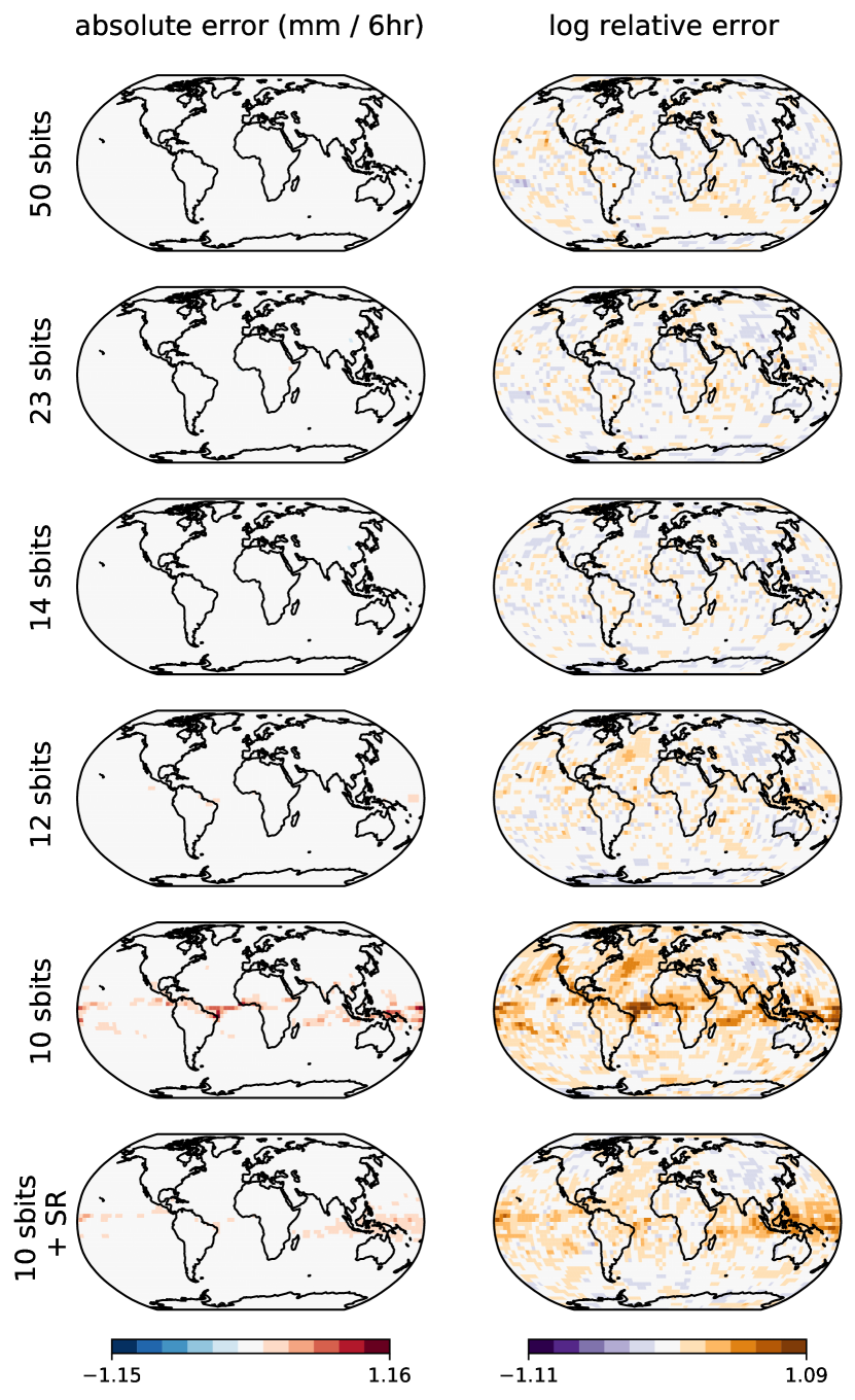
Figure 8: Spatial distribution of precipitation error after 10 years (cf. (4)) & (5))

For both geopotential height and horizontal windspeed we found that rounding error was neglegible relative to high-precision variability for 12 sbits and above, whilst a small rounding error emerged at 10 sbits. For precipitation the picture was similar, except with a very small rounding error emerging at 12 sbits. Fig. 8 reveals those grid points at which rounding error becomes significant relative to high-precision variability for precipitation at 10 sbits. Rounding error is neglegible relative to high-precision variability across all grid points for 14 sbits and above, and the mean high-precision variability for precipitation is around 0.04 mm/6hr which is very small (see A.5 for interpretation of WDs in terms of expected values). Moreover, the rounding error at 10 sbits is small, with grid-point mean values of 0.07 mm/6hr, 5 m and 0.3 m/s for precipitation, geopotential height, and horizontal windspeed respectively, and with the worst affected grid points seeing errors of the order 1 mm/6hr, 25 m and 1 m/s respectively (recall that these values provide bounds on annual means as well as extreme weather events, cf. A.5). To give more intuition behind the size of rounding error at 10 sbits, the probability distributions for precipitation at some of the worst affected tropical grid points (Coastal Suriname 5.56 N, 56.25 W and Western Nigeria 9.27 N, 3.75 E) are plotted in Fig. 9. It is clearly seen that the difference between double and half precision, even at these worst affected grid points, is slight.

It may also be noted from Figs 7 & 8 that stochastic rounding partially mitigates rounding error at half-precision.

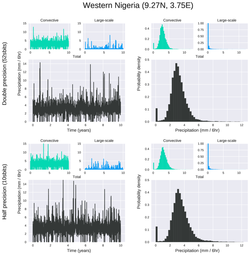
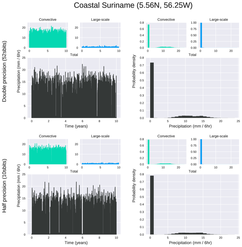
Figure 9: Precipitation climatology at two grid points which are representative of the largest rounding errors at half precision. Even at these worst-affected grid points, the differences between double and half precision are slight.

We also computed differences in annual mean precipitation and found that, by and large, these were of the same order as the GPWDs, indicating that precipitation error was largely accounted for by differences in the means. In general, however, WD bounds are much stronger than mean bounds (cf. Sec. A.5) so we can be confident that our estimates give stringent bounds on rounding error.

6 Conclusions

Whilst there is now convincing evidence that low-precision arithmetic can be suitable for accurate numerical weather prediction, before this work there hadn’t been a detailed study of the effects of rounding error on climate simulations, and we have set out to address this imbalance.

We have argued that an appropriate metric to measure rounding error in the context of a chaotic climate model is the Wasserstein distance (WD), an intuitive and non-parametric metric which provides bounds on a range of expected values including those relevant for extreme weather events. By constructing experiments minimising the variability between probability distributions at high precision and comparing WDs against low precision we have obtained stringent bounds on rounding error, and we have found that error is typically insignificant until truncating as low as half precision in our climate experiments.

We cannot conclude from our results that a state-of-the-art earth system model can be run with equally low precision, since such codes are hugely complex which can make low precision issues difficult to overcome. However, given that the unit round-off error scales exponentially with the number of sbits, it would appear that the current industry standard of double precision across all model components is likely overkill. In terms of acceptable precision, our results for SPEEDY are similar to those found in an analysis of the initial-value problem, suggesting that a level of precision suitable on weather timescales could also be suitable for climate—something which is not obvious a-priori. In light of recent operational successes with single-precision weather forecasting, this is certainly a promising result in the direction of potential single-precision climate modelling.

Regarding stochastic rounding, although not currently in hardware, interest from machine learning together with a number of recently released patents suggest that it might become available soon [3]. Our analysis has shown that stochastic rounding can make models more resilient to rounding error, especially at low precision though theoretically at any precision level, which gives some precedent for the community to engage now with chip-makers to secure the best hardware for next generation models.

Code

For the Lorenz system we made use of github.com/milankl/Lorenz63.jl, for the shallow water model github.com/milankl/ShallowWaters.jl version 0.4 and for SPEEDY we used a branch developed by Saffin for which some changes were made to optimize for low-precision, as documented in [23]. We emulated low-precision using available types in Julia, in particular making use of github.com/milankl/StochasticRounding.jl for stochastic rounding, and we used the reduced precision emulator of [5] in Fortran, for which we developed a custom branch with stochastic rounding. To compute optimal transport distances in 1D we used scipy.stats while for higher dimensional computations including Monte Carlo methods we built a custom solver at github.com/eapax/EarthMover.jl. Additional code gladly provided upon request.

Appendix A The Wasserstein distance

The Wasserstein distance (WD) defines distance between probability distributions $\mu$ and $\nu$ as the lowest cost at which one can transport all probability mass from $\mu$ to $\nu$ with respect to a cost function $c(x,y)=|x-y|^{p}$ which sets the cost to transport unit mass from position $x$ to position $y$, where in our work we have taken $p=1$ so that the WD has the units of the underlying field. In this appendix we will first motivate the WD as a tool for the analysis of climate data by listing some of its favourable properties, before giving the formal definition of the WD, discussing methods for its computation, comparing it with other common metrics, and highlighting its interpretability through a useful dual formulation.

A.1 Properties of the WD

As stated earlier, the WD is defined (at least informally) as the smallest cost required to transport one probability distribution into another. Before giving the formal details of this definition, let us first motivate the WD by lisiting some of its favourable properties.

First, the WD is non-parametric and versatile. It does not require any specific structure of the distributions such as Gaussianity and it can be used to compare both singular and continuous distributions. This is an important point for climate modelling which presents a wide range of probability distributions. For example, the climatological distributions corresponding to South Asian rainfall or the subtropical jet stream latitude are multimodal, while for the Lorenz system the object of interest is a singular probability distribution supported on a fractal attractor. The ability to consider singular distibutions is also useful since it accomodates working directly with the empirical distributions corresponding to a sample of data, rather than first binning the data into a histogram, for example.

Second, the WD is intuitive. It may be interpreted as the minimum amount of work required to transport one distribution into the other, an idea which is readily conceptualised, and it takes the units of the underlying field. For example, for distributions of rainfall measured in mm/day, a WD of 1 can be thought of as a difference of 1mm/day. Moreover, this figure provides bounds on differences in mean rainfall as well as differences in extreme rainfall, for example (cf. A.5).

Third, the WD takes into account geometry. To illustrate this, consider three simple distributions with densities

$$f(x)=\begin{cases}1\quad x\in[0,1]\\ 0\quad\text{otherwise}\end{cases}$$

$$g_{1}(x)=\begin{cases}1\quad x\in[1,2]\\ 0\quad\text{otherwise}\end{cases}$$

$$g_{2}(x)=\begin{cases}1\quad x\in[9,10]\\ 0\quad\text{otherwise.}\end{cases}$$

Now if $f$ is taken as the true distribution and $g_{1}$ & $g_{2}$ as approximations of $f$, then clearly $g_{1}$ gives the better approximation, due to its proximity to $f$. This is reflected with $\text{WD}(f,g_{1})<\text{WD}(f,g_{2})$. By contrast, considering instead the $L^{p}$ distances between densities, for example, would give $\|f-g_{1}\|_{L^{p}}=\|f-g_{2}\|_{L^{p}}=2$ for all $p\geq 1$. which does not reflect the geometry, and this is only intensified in higher dimensions as is illustrated in Fig. 1. This is not just a shortcoming of the $L^{p}$ metric but is shared by measures such as the Kolmogorov-Smirnoff test or the Kullback-Liebler divergence.

More generally, the WD metrises the space of probability distributions with respect to weak convergence [26], which means that closeness in the sense of the WD corresponds to closeness with respect to a natural topology.

A.2 Defining the WD

There are two alternative formulations of optimal transport due to Monge & Kantorovich and it’s helpful to consider both when computing WDs.

For the Monge formulation, suppose we have discrete probability distributions

$$\mu=\frac{1}{N}\sum_{i=1}^{N}\delta_{x_{i}},\quad\eta=\frac{1}{N}\sum_{i=1}^{N}\delta_{y_{i}}$$ (6)

where $x_{i},y_{i}\in\mathbb{R}^{d}$ and we visualize each as a distribution of equal masses on $\mathbb{R}^{d}$. The masses might be books on a bookshelf $\mathbb{R}$ or shipping crates on a dockside $\mathbb{R}^{2}$. We are tasked with transporting $\mu$ to $\eta$. The masses cannot be split so a transport strategy is a permutation $\sigma$ of $N$ objects. Introducing a cost function $c(x,y)$ defining the cost to move unit mass from position $x$ to position $y$, the cost of $\sigma$ is $\frac{1}{N}\sum_{i=1}^{N}c(x_{i},y_{\sigma(i)})$ and the optimal cost is the cost of an optimal strategy $\min_{\sigma\in S_{N}}\left\{\frac{1}{N}\sum_{i=1}^{N}c(x_{i},y_{\sigma(i)})\right\}$ where $S_{N}$ is the set of permutations. The special case $c(x,y)=|x-y|$ defines (Monge’s version of) the WD

$$W_{1}(\mu,\eta)=\min_{\sigma\in S_{N}}\frac{1}{N}\sum_{i=1}^{N}|x_{i}-y_{\sigma(i)}|$$ (7)

Kantorovich’s formulation is a relaxation of Monge’s in that masses are viewed as continuous rather than discrete (think piles of sand rather than shipping crates) so mass can be subdivided in infinitely many ways. Suppose now a pair of distributions

$$\mu=\sum_{i=1}^{M_{1}}P_{i}\delta_{x_{i}},\quad\eta=\sum_{j=1}^{M_{2}}Q_{j}\delta_{y_{j}}$$ (8)

where $\sum_{i}P_{i}=\sum_{j}Q_{j}=1$ and $P_{i},Q_{j}\geq 0$ (i.e. the $P$s and $Q$s are probability vectors). In applications $\mu$ and $\nu$ may represent discrete probability histograms, where the points $x_{i}$ and $y_{j}$ are the mid-points of bins and $P_{i}$ and $Q_{j}$ are weights.

A transport strategy is now defined as a non-negative valued matrix $\pi\in\mathbb{R}^{M_{1}\times M_{2}}_{\geq 0}$ where $\pi_{ij}$ denotes the amount of mass transported from $x_{i}$ to $y_{j}$ and for conservation of mass we impose $\sum_{j}\pi_{ij}=P_{i}$, $\sum_{i}\pi_{ij}=Q_{j}$. Write $c_{ij}$ for the cost to move unit mass from $x_{i}$ to $x_{j}$ so the cost of a strategy is $\sum_{i,j}c_{ij}\pi_{ij}$ and the optimal cost is $\min_{\pi\in\Pi(P,Q)}\sum_{i,j}c_{ij}\pi_{ij}$ where

$$\begin{split}\Pi(P,Q&)=\bigg{\{}\pi\in\mathbb{R}^{M_{1}\times M_{2}}_{\geq 0}\colon\\ &\sum_{j}\pi_{ij}=P_{i},\quad\sum_{i}\pi_{ij}=Q_{j}\bigg{\}}\end{split}$$ (9)

is the set of possible transport strategies. Note that the space $\Pi(P,Q)$ is also the space of joint distributions with marginals $P$ and $Q$, and $\Pi(P,Q)$ is non-empty as can be seen by considering the independence distribution $\pi_{ij}=P_{i}Q_{j}$. The special case $c_{ij}=|x_{i}-y_{j}|$ defines (Kantorovich’s version of) the WD

$$W_{1}(\mu,\nu)=\min_{\pi\in\Pi(P,Q)}\sum_{i,j}|x_{i}-y_{j}|\pi_{ij}$$ (10)

If $M_{1}=M_{2}=N$ and $P_{i}=Q_{j}=\frac{1}{N}$ it may be shown there is a minimizing $\pi$ for (10) which is an optimal strategy in the sense of Monge so (7) and (10) are consistent [26, p5-6].

A.3 Computing the WD

Suppose one has samples $\{x_{i}\}_{i=1}^{N}$ and $\{y_{i}\}_{i=1}^{N}$ drawn from a pair of distributions $\mu$ and $\nu$ on $\mathbb{R}^{d}$. Then one can either compute the Monge WD (7) between the empirical distributions $\mu_{n}=\frac{1}{N}\sum_{i}\delta_{x_{i}}$ and $\eta_{n}=\frac{1}{N}\sum_{i}\delta_{y_{i}}$ directly or one can first perform a data-binning of the data into $M$ bins and compute the Kantorovich WD (10) between the resulting histograms. The complexity of the former scales with the sample size $N$ while the latter scales with the number of bins $M$.

The computation of (7) is a special case of the assignment problem from economics which can be solved in $\mathcal{O}(N^{3})$ by the well-known Hungarian algorithm. On the other hand, the Kantorovich formulation (10) is an example of a problem in linear programming. The set $\Pi(P,Q)$ is a convex polytope and as the cost function is linear it follows that the minimum must be attained on a vertex of this polytope. A minimizing vertex can be found, for example, via the famous simplex algorithm.

When $d=1$ the WD can be computed easily as there is an explicit formula. Indeed, for two 1D distributions with cumulative distribution functions (CDFs) $F$ and $G$ respectively the 1-WD is ([26, p75])

$$W_{1}(F,G)=\int_{-\infty}^{\infty}|F(x)-G(x)|dx.$$ (11)

When $d$ is large data-binning is infeasible and it is more natural to work with the empirical distributions $\mu_{n}$, $\nu_{n}$ directly (resorting to the Monge formulation) however there is a curse of dimensionality in this context. Indeed, one has

$$\mathbb{E}[|W_{1}(\mu_{n},\nu_{n})-W_{1}(\mu,\nu)|]=\mathcal{O}(n^{-\frac{1}{d}})$$

and this bound is sharp in general which gives very slow convergence in high dimension in some cases [8]. Construction of a metric to rival the WD which does not suffer a curse of dimensionality is an open problem and active research.

In our work we have found that, despite the curse of dimensionality, computating the WD between empirical distributions with a modest sample size is computationally feasible and provides a useful checksum, usually in agreement with results obtained for example by marginalising on one-dimensional subspaces. We also note that interesting recent work has shown a regularised form of the WD called the Sinkhorn divergence (SD) [4] has improved sample complexity with a dimension agnostic convergence rate of $\mathcal{O}(n^{-\frac{1}{2}})$ for appropriate regularising parameters [9] and in our work we found that many WD computations could be corroborated by SDs provided a suitable choice of regularising parameter was chosen to ensure convergence of the Sinkhorn algorithm.

A.4 Comparing other metrics

It is interesting to note the similarity between (11) and the Continuous Rank Probability Score often used for weather forecast skill

$$\mathrm{CRPS}(F,G)=\int_{-\infty}^{\infty}|F(x)-G(x)|^{2}dx$$ (12)

and with the Kolmogorov-Smirnoff test

$$\mathrm{KS}(F,G)=\sup_{x\in(\infty,\infty)}|F(x)-G(x)|$$ (13)

for CDFs $F$ and $G$. For the WD with $p=2$ cost there is the explicit formula in 1D

$$W_{2}(F,G)=\int_{-\infty}^{\infty}|F^{-1}(x)-G^{-1}(x)|^{2}dx$$ (14)

where $F^{-1}$ and $G^{-1}$ are generalized inverses [26, p.75]. Note that (11), (12) and (14) take account of the geometry of $\mathbb{R}$ (cf. A.1) while (13) does not.

A.5 Duality.

Suppose we have a pair of distributions $\mu$ and $\nu$ representing, for example, rainfall at a fixed location in mm/6hr. How can we interpret a WD of, say, 1 between $\mu$ and $\nu$?

Since cost is defined as $c(x,y)=|x-y|$ a nice property of the WD is that it inherits the units of rainfall so that we can interpret the difference in mm/6hr. Heuristically, this difference tells us that a cost of at least 1mm/6hr must be spent to transport $\mu$ to $\nu$, and this takes into account both mean and extreme rainfall.

Moreover, this distance gives bounds on a range of expected values by the Kantorovich-Rubenstein duality [26, Thm 1.14] which states

$$W_{1}(\mu,\nu)=\sup_{f\in\mathrm{Lip}_{1}}\left|\mathbb{E}[f(X_{\mu})]-\mathbb{E}[f(Y_{\nu})]\right|$$

where $X_{\mu}$ and $Y_{\nu}$ are random variables with laws $\mu$ and $\nu$ and $\mathrm{Lip}_{1}$ is the space of functions satisfying $|f(x)-f(y)|\leq|x-y|$ (the 1-Lipschitz functions). Taking $f(x)=x$ and duality gives

$$\left|\mathbb{E}[X_{\mu}]-\mathbb{E}[Y_{\nu}]\right|\leq W_{1}(\mu,\nu)$$

which shows that a WD of $1$mm/6hr implies a difference in expected rainfall of less than 1mm/6hr (note this bound is sharp when $\mu$ and $\nu$ are Dirac masses). But duality also gives bounds on expected extreme rainfall. To see this, suppose extreme rainfall is defined as any rainfall which falls in excess of $r_{c}$ mm/6hr where $r_{c}$ is some critical value. Then taking $f(x)=0$ for $x<r_{c}$ and $f(x)=x-r_{c}$ for $x\geq r_{c}$ gives

$$\left|\mathbb{E}[f(X_{\mu})]-\mathbb{E}[f(Y_{\nu})]\right|\leq W_{1}(\mu,\nu)$$

which shows a difference in expected extreme rainfall of $\leq 1$mm/6hr.

Understanding such heuristics is helpful in interpreting the bounds on rounding error derived in this paper.

Appendix B Number formats

B.1 Floating-point arithmetic

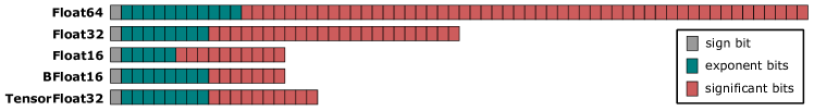
Figure 10: Floating-point number formats available in hardware. The IEEE754 standard for Float64 is 1 sign bit, 11 exponent bits and 53 significant bits, whilst Float32 and Float16 break down as (1, 8, 23) and (1, 5, 10) respectively. Google’s BFloat16 format (the B stands for Brain) opts for a (1, 8, 7) split, sacrificing precision for a larger dynamic range, while NVidia’s new TensorFloat32 is (1, 8, 10) retaining the precision of Float16 but with the dynamic range of Float32.

The standard arithmetic format for scientific computing is the floating-point number (float). The bits in a float are divided into three groups: a sign bit, the exponent bits, and the significant bits. A non-zero exponent specifies an interval $I=[2^{e-\text{bias}},2^{e+1-\text{bias}})$ with a bias to allow for negative exponents while the exponent bits are interepreted as an unsigned integer $e$. For $e=0$, floats are defined on an interval $I=(0,\pm 2^{1-\text{bias}})$ called the subnormal range. The signficant bits specify a point on $I$ from an evenly-spaced partition of $I$. Thus, for a given bias, the number of exponent bits determine the dynamic range of representable numbers in the normal range, while the subnormal range, and therefore the smallest representable number, is determined by the number of significant bits. Some different float formats available in hardware are shown in Fig. 10.

The IEEE-754 Float64 format is called double precision, and Float32 and Float16 single and half precision respectively.

B.2 Rounding

The default rounding mode for floats is round-to-nearest tie-to-even (RN) which rounds an exact result $x$ to the nearest representable number $x_{i}$. In case $x$ is half-way between two representable numbers, the result will be tied to the even float, whose significand ends in a zero bit. These special cases are therefore alternately round up or down, which removes a bias that would otherwise persist.

For stochastic rounding (SR) rounding of $x$ down to a representable number $x_{1}$ or up to $x_{2}$ occurs at probabilities that are proportional to the respective distances. Specifically, if $u$ is the distance between $x_{1},x_{2}$, then $x$ will be rounded to $x_{1}$ with probability $1-u^{-1}(x-x_{1})$ and to $x_{2}$ with probability $u^{-1}(x-x_{1})$.

The introduced absolute rounding error for SR is always at least as big as for RN and when low-probability round away from nearest occurs, it can be up to $\pm u$, twice as large as for round-to-nearest. However, by construction, SR is exact in expectation and thus in particular by the law of large numbers one has

$$\lim_{N\to\infty}\frac{1}{N}\sum_{i=1}^{N}\text{stochastic\leavevmode\nobreak\ round}(x)=x$$

with the limit obtained in the strong sense. Moreover, by sometimes rounding small remainders up, rather than always rounding them down as in RN, systemic errors can sometimes be avoided with SR, such as in stagnation (see Sec. 4 for an example).

It is worth noting that SR at low precision requires computation at a higher precision in order to generate the probabilities for rounding, however all numbers are written, read, and communicated at low precision. It is also interesting to note that SR can easily be implemented with a random number sampled from the uniform distribution, which can thus be done in parallel to the arithmetic.

References

- [1] M. Arjovsky, S. Chintala, and L. Bottou. Wasserstein generative adversarial networks. In Proceedings of the 34th International Conference on Machine Learning, volume 70, pages 214–223, 2017.
- [2] M. Chantry, T. Thornes, T. Palmer, and P. Düben. Scale-selective precision for weather and climate forecasting. Monthly Weather Review, 147(2):645–655, Jan. 2019.
- [3] M. Croci and M. B. Giles. Effects of round-to-nearest and stochastic rounding in the numerical solution of the heat equation in low precision, 2020.
- [4] M. Cuturi. Sinkhorn distances: Lightspeed computation of optimal transport. In Advances in Neural Information Processing Systems 26, pages 2292–2300. 2013.
- [5] A. Dawson and P. Düben. rpe v5: An emulator for reduced floating-point precision in large numerical simulations. Geoscientific Model Development Discussions, pages 1–16, 11 2016.
- [6] A. Dawson, P. D. Düben, D. A. MacLeod, and T. N. Palmer. Reliable low precision simulations in land surface models. Climate Dynamics, 51(7):2657–2666, 2018.
- [7] M. M. Dogar, F. Kucharski, and S. Azharuddin. Study of the global and regional climatic impacts of enso magnitude using speedy agcm. Journal of Earth System Science, 126(2), 2017.
- [8] R. M. Dudley. The speed of mean Glivenko-Cantelli convergence. Ann. Math. Statist., 40(1):40–50, 02 1969.
- [9] A. Genevay, L. Chizat, F. Bach, M. Cuturi, and G. Peyré. Sample complexity of sinkhorn divergences. In Proceedings of Machine Learning Research, volume 89, pages 1574–1583, 2019.
- [10] R. Gilham. 32-bit Physics in the Unified Model. Technical Report 626, Met Office, Exeter, UK, 2018.
- [11] S. Gupta, A. Agrawal, K. Gopalakrishnan, and P. Narayanan. Deep learning with limited numerical precision. In Proceedings of the 32nd International Conference on Machine Learning, volume 37 of ICML’15, pages 1737–46. JMLR.org, 2015.
- [12] R. Harvey and D. L. Verseghy. The reliability of single precision computations in the simulation of deep soil heat diffusion in a land surface model. Climate Dynamics, 46(11):3865–3882, 2016.
- [13] S. Hatfield, M. Chantry, P. Düben, and T. Palmer. Accelerating high-resolution weather models with deep-learning hardware. In Proceedings of the Platform for Advanced Scientific Computing Conference, 2019.
- [14] S. Jeffress, P. Düben, and T. Palmer. Bitwise efficiency in chaotic models. Proceedings of the Royal Society A: Mathematical, Physical and Engineering Sciences, 473(2205):20170144, Sept. 2017.
- [15] M. Klöwer, P. D. Düben, and T. N. Palmer. Number formats, error mitigation, and scope for 16-bit arithmetics in weather and climate modeling analyzed with a shallow water model. Journal of Advances in Modeling Earth Systems, 12(10), Oct. 2020.
- [16] F. Kucharski, F. Molteni, M. P. King, R. Farneti, I.-S. Kang, and L. Feudale. On the need of intermediate complexity general circulation models: A “SPEEDY” example. Bulletin of the American Meteorological Society, 94(1):25–30, Jan. 2013.
- [17] E. N. Lorenz. Deterministic Nonperiodic Flow. Journal of the Atmospheric Sciences, 20(2):130–141, 03 1963.
- [18] C. Maass. ECMWF Implementation of IFS cycle 47r2. 2021.
- [19] P. Micikevicius, S. Narang, J. Alben, G. Diamos, E. Elsen, D. Garcia, B. Ginsburg, M. Houston, O. Kuchaiev, G. Venkatesh, and H. Wu. Mixed precision training. In International Conference on Learning Representations, 2018.
- [20] F. Molteni and F. Kucharski. A heuristic dynamical model of the North Atlantic Oscillation with a Lorenz-type chaotic attractor. Climate Dynamics, 52(9-10):6173–6193, Oct. 2018.
- [21] Y. Robin, P. Yiou, and P. Naveau. Detecting changes in forced climate attractors with wasserstein distance. Nonlinear Processes in Geophysics, 24(3):393–405, 2017.
- [22] S. Rüdisühli, A. Walser, and O. Fuhrer. COSMO in single precision. COSMO Newsletter No. 14, 2014.
- [23] L. Saffin, S. Hatfield, P. Düben, and T. Palmer. Reduced-precision parametrization: lessons from an intermediate-complexity atmospheric model. Quarterly Journal of the Royal Meteorological Society, 146(729):1590–1607, Feb. 2020.
- [24] W. Tucker. A rigorous ODE solver and Smale’s 14th problem. Found. Comput. Math., 2(1):53–117, 2002.
- [25] F. Váňa, P. Düben, S. Lang, T. Palmer, M. Leutbecher, D. Salmond, and G. Carver. Single precision in weather forecasting models: An evaluation with the IFS. Monthly Weather Review, 145(2):495–502, Feb. 2017.
- [26] C. Villani. Topics in Optimal Transportation. Graduate studies in mathematics. American Mathematical Society, 2003.
- [27] G. Vissio, V. Lembo, V. Lucarini, and M. Ghil. Ranking IPCC Models Using the Wasserstein Distance. arXiv e-prints, page arXiv:2006.09304, June 2020.
- [28] G. Vissio and V. Lucarini. Evaluating a stochastic parametrization for a fast–slow system using the wasserstein distance. Nonlinear Processes in Geophysics, 25(2):413–427, June 2018.