Black-box Gradient Attack on Graph Neural Networks: Deeper Insights in Graph-based Attack and Defense

Abstract.

Graph Neural Networks (GNNs) have received significant attention due to their state-of-the-art performance on various graph representation learning tasks. However, recent studies reveal that GNNs are vulnerable to adversarial attacks, i.e. an attacker is able to fool the GNNs by perturbing the graph structure or node features deliberately. While being able to successfully decrease the performance of GNNs, most existing attacking algorithms require access to either the model parameters or the training data, which is not practical in the real world.

In this paper, we develop deeper insights into the Mettack algorithm, which is a representative grey-box attacking method, and then we propose a gradient-based black-box attacking algorithm. Firstly, we show that the Mettack algorithm will perturb the edges unevenly, thus the attack will be highly dependent on a specific training set. As a result, a simple yet useful strategy to defense against Mettack is to train the GNN with the validation set. Secondly, to overcome the drawbacks, we propose the Black-Box Gradient Attack (BBGA) algorithm. Extensive experiments demonstrate that out proposed method is able to achieve stable attack performance without accessing the training sets of the GNNs. Further results shows that our proposed method is also applicable when attacking against various defense methods.

1. Introduction

Graph structured data is widely used in a variety of domains, such as social networks(Wasserman and Faust, 2007), academic publishing(Fricke, 2018), recommender systems(Ying et al., 2018) and financial transactions(Ron and Shamir, 2013). How to learn effective graph representations has long been an important research direction. Recently, Graph Neural Networks (GNNs) has become the mainstream method for graph representation learning(Zhou et al., 2018). Firstly introduced by (Scarselli et al., 2009), the Graph Convolutional Network (GCN)(Kipf and Welling, 2017) achieved state-of-the-art performance in the node-classification task and is considered as the most representative GNN model. Then, numerous GNN models, such as GAT(Velickovic et al., 2018), GraphSAGE(Hamilton et al., 2017) and JK-Net(Xu et al., 2018), have been proposed.

It has been revealed that deep learning models are often in lack of robustness(Goodfellow et al., 2015). It is possible to fool the model by generating perturbations deliberately. GNNs are no exceptions. Adversarial attacks on GNNs could be classified using various criteria. According to the attackers’ knowledge, we could divide existing GNN attacks into white-box attacks, grey-box attacks and black-box attacks(Chen et al., 2020). In the white-box scenario, the adversary has access to both the model parameters and the training data, which even include the ground-truth labels. Grey-box attacks only need partial information and they are more practical than the white-box ones. Representative grey-box attacking methods include Nettack(Zügner et al., 2018), which aims to misclassify a set of targeted nodes, and Mettack(Zugner and Gunnemann, 2019), which aims to reduce the overall classification accuracy rates. Since model parameters are not accessible in grey-box scenarios, a surrogate model is usually trained on the training set to approximate the gradients of potential perturbations. Black-box attacks allow the most limited knowledge such that only black-box queries are possible(Sun et al., 2018). Since the access to the training set is also prohibited, reinforcement learning is introduced to perform black-box attacks(Jin et al., 2020a). However, the queries are still considered to be impractical and RWCS, a black-box attack based on the theory of random walk, has been proposed(Ma et al., 2020).

Various defense methods have also been proposed. For instance, GCN-Jaccard (Wu et al., 2019) increases the robustness of GCNs by eliminating edges with low similarity before the training process. R-GCN (Zhu et al., 2019) utilizes the attention mechanism which regards node features as Gaussian distributions and assigns attention scores according to the variances. By introducing structure learning, Pro-GNN(Jin et al., 2020b) achieves promising results when defending against structure perturbations.

Although defense algorithms have emerged to enhance the security of GNNs, studies on deep learning models show that it is possible to improve the adversarial attacks to degrade the defense performance(Athalye et al., 2018; Carlini and Wagner, 2017). Meanwhile, in-depth studies on adversarial attacks is an efficient tool to develop insights in deep learning models(Geirhos et al., 2019). Comparing with Deep Neural Networks (DNNs), adversarial attacks on GNNs remain poorly understood.

One perspective to improve adversarial attacks is to understand how existing attacks work at first. In this paper, we target on investigate Mettack, which is the most representative non-targeted grey-box attack, to develop a deeper understanding of graph attack and defense. Our case studies show that the perturbations chosen by Mettack are highly correlated with the training set and they are distributed unevenly on the graph. As a result, we reveal that a simple defense strategy is to train the GNN with the validation set. Based on the findings, we propose the Black-Box Gradient Attack (BBGA) algorithm to evenly perturb the graphs without accessing any ground-truth labels. Extensive experiments on three real-world benchmark datasets demonstrate that our proposed method can effectively attack the graph structure without accessing any training labels.

In summary, our contributions of this paper are as follows:

• How Mettack works: We studies the patterns of Mettack perturbations and we show that the perturbations are denser near the training set. We show that such unevenness helps in grey-box attacks but it could also be utilized by defenders.

• Black-box Gradient Attack (BBGA): While it is believed that training surrogate model without ground-truth labels are impossible, we propose the first gradient-based black-box attacking method to our best knowledge. It is also the first non-targeted graph structure attack without permission to do black-box queries. Exploiting the spectral clustering, we train the surrogate model with pseudo-labels and then evenly distribute the perturbations via a novel $k$-fold training strategy.

• Extensive experiments: We conduct numerous experiments to show the effectiveness of our proposed method. Further studies are provided for the explanability of the method.

The rest of our paper is organized as follows. In Section 2, we define the mathematical notations used in this paper and then we introduce the preliminaries. In Section 3, we analyse Mettack perturbations via a series of case studies. In Section 4, we introduce our propose BBGA method and explain it in details. Experimental results, ablation studies and parameter analysis are reported in Section 5. Finally, we conclude the paper in Section 6.

2. Preliminaries

In this section, we introduce the notations used in this paper as well as fundamental concepts.

2.1. Mathematical Notations

In this paper, we denote a graph with $N$ nodes as $G=(V,E)$ where $V=\{v_{1},\cdots,v_{N}\}$ is the node set and $E=\{e_{1},\cdots,e_{E}\}\subseteq V\times V$ is the edge set. The set of vertices $V$ is usually divided into the training set $V_{\text{train}}$, the validation set $V_{\text{val}}$ and the testing set $V_{\text{test}}$. We denote the structure of the $G$ via the adjacency matrix $A\in\{0,1\}^{N\times N}$ whose element $A_{ij}=1$ if and only if $\exists i\in[1,E]\text{ s.t. }e_{i}\in E$ connects $v_{i}$ and $v_{j}$. Node features are stored in a matrix $X\in\mathbb{R}^{N\times F}$ where $F$ is the number of dimensions of node features. The labels of a dataset is denoted by $C$ while pseudo-labels used during training are denoted as $C_{p}$.

2.2. Graph Convolutional Networks(GCNs)

Despite a number of GCN models have been proposed, in this paper we mainly consider the most representative one introduced by (Kipf and Welling, 2017). Each layer of a GCN aggregate messages according to the graph structure and then perform linear transformation on the node features. Such a graph convolutional layer could be denoted as the following equation:

(1) $$H^{(l+1)}=\sigma(\hat{A}H^{(l)}W^{(l)}),$$

where $\hat{A}=\tilde{D}^{-\frac{1}{2}}\tilde{A}\tilde{D}^{-\frac{1}{2}}$ is the normalized adjacency matrix such that $\tilde{A}=A+I_{N}$, $\tilde{D}_{i,i}=\sum_{j}\tilde{A}_{i,j}$. $\sigma$ is a non-linear activation function. A typical GCN network consists of two layers, the whole network is usually described as:

(2) $$Z=f(X,A)=\text{softmax}(\hat{A}\sigma(\hat{A}XW^{(0)})W^{(1)}).$$

The GCN network is usually trained with a cross entropy loss. Noticing that two-layer GCNs aggregate information within 2-hop neighborhoods for each node, a simplified and linearized version is usually used in adversarial attacks:

(3) $$Z=f(A,X)=\text{softmax}(\hat{A}^{2}XW).$$

To utilize GCN in inductive settings, (Hamilton et al., 2017) introduced a variant of GCN with a different normalization method:

(4) $$h_{v}^{(l)}=\sigma\left(W_{l}\cdot\frac{1}{\tilde{D}_{(v,v)}}\sum_{u\in\tilde{\mathcal{N}}(v)}h_{u}^{(l-1)}\right),$$

where $h_{v}^{(l)}$ is the hidden representation of node $v$ in the $l^{th}$ layer and $\tilde{\mathcal{N}}(v)$ is the neighborhood of node $v$ in the self-looped graph with $\tilde{A}$ as the adjacency matrix.

2.3. Mettack

Mettack(Zugner and Gunnemann, 2019) is a gradient-based grey-box graph attacking algorithm. Being directly connected to the training loss, gradients are widely used in deep learning adversarial attacks(Yuan et al., 2019). Being denied to access model parameters, Mettack trains the surrogate model described in Eq. 3 to approximate the gradients of the GCN model. In order to find the best edge to perturb, the adjacency matrix is regarded as a hyperparameter and the meta-gradients are computed after the training of the surrogate model:

(5) $$\nabla_{G}^{\text{meta}}:=\nabla_{G}\mathcal{L}_{\text{atk}}(f_{\theta^{*}}(G))\text{ s.t. }\theta^{*}=\text{opt}_{\theta}(\mathcal{L}_{\text{train}}(f_{\theta}(G))),$$

where $\mathcal{L}_{\text{atk}}$ is the target function that the attacker aims to optimize, opt is a training procedure and $\mathcal{L}_{\text{train}}$ is the training loss. It is revealed that when $\mathcal{L}_{\text{atk}}=-\mathcal{L}_{\text{self}}$, where $\mathcal{L}_{\text{self}}$ is the cross-entropy loss on the unlabelled nodes with predicted pseudo-labels, the algorithm reaches its best performance.

A greedy algorithm, which chooses exactly one edge a step, is employed to perform perturbations. The score of a node pair $(u,v)$ is defined as:

(6) $$S(u,v)=\nabla_{A_{uv}}^{\text{meta}}\cdot(-2\cdot A_{uv}+1),$$

where $A$ is the adjacency matrix. The signs of meta-gradients are flipped for connected node pairs to yields the gradients for removing the edge. In each iteration, the algorithm picks the potential perturbation with the highest score.

The total number of perturbations is controlled by a budget constraint $\Delta$, which is usually defined via a perturbation rate $\delta=\frac{\Delta}{|E|}$.

3. Case studies on Mettack

Adversarial attacks generate deliberate perturbations on graph data. Hence, to investigate why adversarial attacks work, it is necessary to analyse the perturbations made by attacking algorithms. Previous studies find out that dissimilar nodes tend to be connected by attackers(Wu et al., 2019). In this paper, we focus on the distributions of such carefully-crafted perturbations.

3.1. Unevenness of perturbations

Consisting of 2 graph convolutional layers, a typical GCN network is only able to aggregate information with the 2-hop neighborhood of each node. Xu et al. proved the following theorem:

Theorem 3.1 ((Xu et al., 2018)).

If all paths in the computation graph of the model are activated with the same probability. Given a L-layer GCN with Eq. 4 as the normalization method, then $\forall i,j\in V$, $\mathbb{E}[\frac{\partial H_{j}}{\partial X_{i}}]$ is equivalent to the probability of reaching node $j$ via a k-step random walk starting at node $i$.

Inspired by Theorem 3.1, it is nature to raise the question that whether grey-box gradient attacks mainly perturb edges that are adjacent to the training set or not.

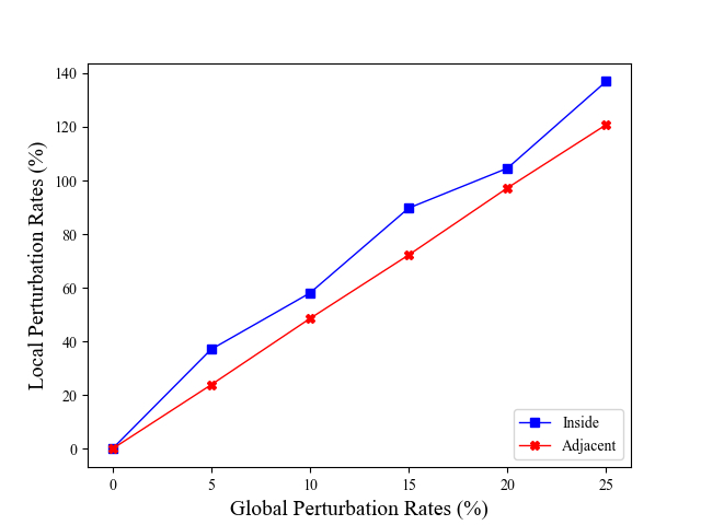
The local perturbations rates of mettack perturbed graphs.

Figure 1. The local perturbations rates of mettack perturbed graphs.

We conducted a case study on the Cora dataset with Mettack. Figure 1 demonstrates the local perturbation rates both inside and adjacent to the training set. As illustrate in the figure, the local perturbation rate inside the training set exceeds $100\%$ when the global perturbation rate reaches $20\%$. Considering the edges $(v_{1},v_{2})$ that are adjacent to the training set such that

(7) $$(v_{1}\in V_{\text{train}}\land v_{2}\not\in V_{\text{train}})\lor(v_{1}\not\in V_{\text{train}}\land v_{2}\in V_{\text{train}}),$$

the local perturbation rate exceeds $100\%$ when the global perturbation rate reaches $25\%$. Thus, instead of perturbing the edges evenly, Mettack essentially flips a much higher proportion of edges near the training set than the assigned perturbation rate.

3.2. Ablation Study on The Unevenness

In order to show the effects of such unevenness, an ablation study on the Cora dataset is conducted. We create two variants of the DICE (Disconnect Internally, Connect Externally) algorithm, which disconnects nodes with the same label and connects nodes with different labels randomly. DICE-Free randomly flips edges on the whole graph. DICE-Control ensures that $10\%$ of the perturbations are within the training set and $90\%$ of the flips are adjacent to the training set. Following (Zugner and Gunnemann, 2019), we suppose that the attacker knows all the ground-truth labels in this study.

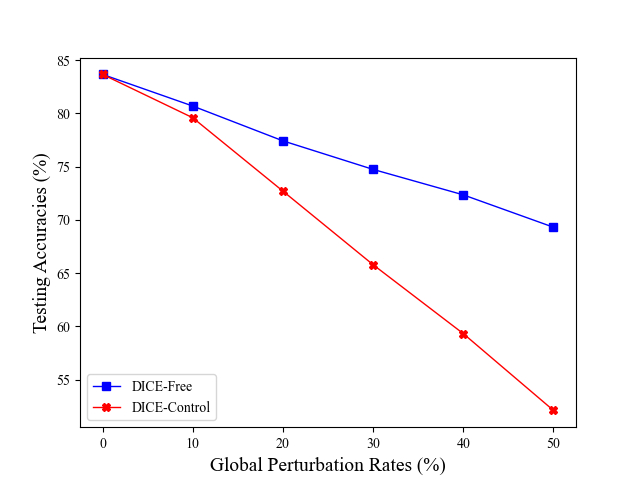
The testing accuracies of GCN on DICE-attacked graphs.

Figure 2. The testing accuracies of GCN on DICE-attacked graphs.

As reported in Figure 2, the enforced unevenness does not boost the attacking performance too much when perturbation rates are low. However, with the increasing of perturbation rates, DICE-Control outperforms DICE-Free significantly. When the perturbation rates are $50\%$, DICE-Control leads to a $56.05\%$ higher misclassification rate than DICE-Free. The result demonstrates that when the training set is accessible, the unevenness of perturbations helps a lot in grey-box adversarial attacks.

3.3. Defend Mettack via Validation Set

Ptb Rate	GCN	Flip-GCN
10%	71.59$\pm$1.79	81.19$\pm$0.89
20%	55.88$\pm$5.03	80.50$\pm$0.69

Table 1. The experimental results of the flip strategy (Accuracy$\pm$Std).

Although the unevenness helps in attacking, it could also be utilized by the defender. We develop Flip-GCN, which is a training strategy that trains the GCN with the validation set, to defend against Mettack. Following the experimental settings of (Jin et al., 2020b), we randomly select 10% of nodes as the training set, 10% for validation and the remaining 80% as the testing set. The graph is perturbed by Mettack without the log-likelihood restraint. As reported in Table 1, when $V_{\text{train}}$ and $V_{\text{val}}$ are flipped, the testing accuracy increased dramatically.

4. Black-Box Gradient Attack

As demonstrated by the above studies, Mettack has the tendency to perturb the edges unevenly. While such unevenness contributes to the performance, it is in lack of robustness since even training the GCN with the validation set will degrade its performance severely. Meanwhile, the tendency to connect dissimilar nodes are also easily utilized by defense algorithms (Jin et al., 2020b; Wu et al., 2019).

To increase the robustness of adversarial attacks, the perturbations should be unbiased to any data splits. Thus, indeed the attack is supposed to be black-box to prevent such biases.

While most black-box attacks are based on reinforcement learning (Dai et al., 2018; Ma et al., 2019), random walk-based attacks such as RWCS are also promoted recently to avoid model inquires (Ma et al., 2020). However, RWCS focuses on perturbing features instead of graph structures. To our best knowledge, no existing structure-oriented black-box attack works without black-box inquires. Meanwhile, gradients are not exploited in black-box attacks since a surrogate model is needed. However, gradients are powerful tools to pick edges for perturbations. In this paper, by disengaging gradients from any specific training set, we propose the novel Black-Box Gradient Attack (BBGA) algorithm.

4.1. Attack Condition

In this subsection, we introduce the attacking condition of our model systematically.

Goal: As an untargeted attack, the attacker’s goal is to decrease the classification accuracies of GNNs.

Knowledge: As a black-box attack, the access to model parameters, training data and ground-truth labels are denied. The graph $G=(V,E)$ and the node features are considered to be accessible.

Constraints: The number of changes is restricted by a budget $\Delta$ such that $\lVert A^{\prime}-A\rVert_{0}\leq 2\Delta$. Here $A^{\prime}$ is the modified adjacency matrix and we have $2\Delta$ due to the symmetry of adjacency matrices. In addition, various defense algorithms have taken advantage of the connections between dissimilar nodes (Wu et al., 2019; Jin et al., 2020b). We believe that such easily-detected modifications are supposed to be restricted since they could be easily eliminated by a pre-processing algorithm. Noticing that node features in common graph tasks are encoded in the one hot manner, we propose a similarity constraint such that for any pair of nodes $v_{1},v_{2}\in V$, if their Jaccard similarity score $J_{v_{1},v_{2}}$ is smaller than a threshold value $\eta$, the connection of $v_{1}$ and $v_{2}$ is disallowed. The definition of Jaccard similarity score is:

(8) $$J_{v_{1},v_{2}}=\frac{M_{11}}{M_{01}+M_{10}+M_{11}},$$

where $M_{ab}(a,b\in\{0,1\})$ represents the number of features which have value $a$ in node $v_{1}$ and value $b$ in node $v_{2}$. The constrains are summarized as a function $\phi(G):G\rightarrow\mathcal{P}(V\times V)$, where $G$ is the graph to attack. The function $\phi$ maps the graph to a set of valid node pairs.

4.2. Pseudo-label and Surrogate Model

Since no ground-truth labels are accessible, pseudo-labels are needed in order to train the surrogate model. We utilize spectral clustering to generate pseudo-labels(Pedregosa et al., 2011). Parameters of the spectral clustering algorithm are chosen according to the Calinski-Harabasz Score.

Since it’s not accurate to approximate the gradients of GNNs with pseudo-labels generated by a spectral clustering algorithm, a simplified GCN described in 3 is employed as the surrogate model. The surrogate model is trained with the pseudo-labels on a random training set, which has no relation with the training set of the defense model.

4.3. $k$-Fold Greedy Attack

As demonstrated in Section 2, a main drawback of Mettack is the uneven distribution of the modifications. In the black-box scenario in which the training set is not accessible, the attacker is supposed to distribute its modifications in the whole graph. In this paper, we proposed a novel $k$-fold greedy algorithm to solve this problem.

We divide the node set $V$ into $k$ partitions $V_{1},V_{2},\cdots,V_{k}$. For the $i^{\text{th}}$ partition $V_{i}(i\in[1,k])$, we predict $\hat{C}_{i}$, which is the labels of nodes in $V-V_{i}$, with a GCN trained on it. The attacker loss function is defined as:

(9) $$\mathcal{L}_{\text{atk}}^{i}=-\mathcal{L}(V-V_{i},\hat{C}_{i}),$$

where $\mathcal{L}$ is the cross-entropy loss.

With the attacker’s loss, we compute the meta-gradients (gradients w.r.t. hyperparameters):

(10) $$\nabla_{G}^{i}:=\nabla_{G}\mathcal{L}_{\text{atk}}^{i}(f_{\theta^{*}}(G))\text{ s.t. }\theta^{*}=\text{opt}_{\theta}(\mathcal{L}_{i}(f_{\theta}(G))),$$

where $\mathcal{L}_{i}$ is the cross-entropy loss on partition $V_{i}$. Similar to Mettack, the partition score function $S^{i}:V\times V\rightarrow\mathbb{R}$ on the $i^{th}$ partition is defined as:

(11) $$S^{i}(u,v)=\nabla_{u,v}^{i}\cdot(-2\cdot A_{uv}+1).$$

For each pair of node $(u,v)$, we compute $\sigma_{uv}$, which is the standard deviation of its $k$ partition scores. The greedy score for $(u,v)$ is defined as:

(12) $$S(u,v)=\begin{cases}\sum_{i=1}^{k}S^{i}(u,v),\text{ }&\sigma_{uv}<\tilde{\sigma}\\ 0,\quad&(\sigma_{uv}>=\tilde{\sigma})\lor(u=v)\end{cases}$$

where $\tilde{\sigma}$ is the median of all $\sigma_{uv}$s. The definition eliminates all self-loops and ensures that the gradients of the chosen perturbation on the $k$ partitions are not too diverse.

In each step, we greedily pick exactly one perturbation $e^{\prime}=(u^{\prime},v^{\prime})$ with the highest score:

(13) $$e^{\prime}=\mathop{\arg\max}_{e=(u,v)\in\phi(G)}S(u,v),$$

where $e\in\phi(G)$ ensures that the modification does not conflict with the attack constraints. Then the algorithm updates $G$ according to $e^{\prime}=(u^{\prime},v^{\prime})$ by flipping the value of $A_{u^{\prime}v^{\prime}}$.

4.4. Algorithm

Algorithm 1 Black-Box Gradient Attack (BBGA)

Input: $G=(V,E)$, node features $X$, attack budget $\Delta$, constraint $\phi(G)$, training iteration $T$, partition $\{V_{1},\cdots,V_{k}\}$.
Output: Modified graph $G^{\prime}=(V,E^{\prime})$.

1:  $C_{p}$ $\leftarrow$ SpectralClustering$(G,X)$.

2:  $C_{s}$ $\leftarrow$ training surrogate model with $C_{p}$ and a random training set.

3:  $A^{\prime}$ $\leftarrow$ $A$

4:  while $\lVert A^{\prime}-A\rVert_{0}<2\Delta$ do

5:     for $i\in[1,k]$ do

6:        randomly initialize $\theta_{0}$;

7:        $\theta_{T}$ $\leftarrow$ update parameters for $T$ iterations;

8:        $\nabla_{G}^{i}\leftarrow\nabla_{G}\mathcal{L}_{\text{atk}}^{i}(f_{\theta^{T}}(G))$;

9:        $S_{i}\leftarrow\nabla_{G}^{i}\odot(-2A^{\prime}+1)$;

10:     end for

11:     $S$ $\leftarrow$ according to Eq. 12;

12:     $e^{\prime}\leftarrow$ the index of the maximum element in $S$ that are in $\phi(G)$;

13:     $A^{\prime}\leftarrow$ flip edge $e^{\prime}$.

14:  end while

15:  $G^{\prime}$ $\leftarrow$ use $A^{\prime}$ as the new adjacency matrix; return: $G^{\prime}$.

Following the detailed description, we now present the pseudo-code of the BBGA algorithm in Algorithm 1.

The meta-gradients of all the $N^{2}$ pairs of nodes will be computed in the algorithm, the computing of meta-gradients have $T$ steps due to the chain rule and the meta-gradients are calculated for each of the $k$ partitions. Thus, the computational complexity for the attacking procedure itself is bounded by $O(k\cdot T\cdot N^{2})$. Considering the computational efforts needed to find the pseudo-labels(Yan et al., 2009), the overall computational complexity of BBGA is $O(k\cdot T\cdot N^{2})+O(n^{3})$.

5. Experiments

In this section, we evaluate our proposed BBGA algorithm against both vanilla GCN and several defense methods.We introduce our experimental settings at first and then we aim to answer the following research questions:

• RQ1: How does BBGA works without accessing the training set of the model?

• RQ2: Are the attacked graph as expected such that the perturbations are not distributed mainly around the training set?

• RQ3: How do different components and hyperparameters affect the performance of BBGA?

5.1. Experimental Settings

5.1.1. Datasets

Dataset	$|V|$	$|E|$	Classes	Features
Cora	2485	5069	7	1433
Citeseer	2110	3668	6	3703
Cora-ML	2810	7981	7	2879

Table 2. Statistics of datasets. Notice that only the largest connected components of the graphs are considered.

Cora, Citesser and Cora-ML, which are threecommonly-used real-world benchmark datasets, are employed in our experiments. Following (Zugner and Gunnemann, 2019), we only consider the largest connected components of the graphs. The statistics of the datasets are summarized in Table 2. Following (Jin et al., 2020b), we randomly pick 10% of nodes for training, 10% of nodes for validation and the remaining 80% of nodes for testing.

5.1.2. Defense Methods

To demonstrate the effectiveness of our proposed BBGA method, both vanilla GCN and several defense algorithms are employed in our experiments. For GCN and RGCN we use the official implementation along with its hyperparameters. For other models we use the implementation and hyperparatemers in (Li et al., 2020).

• GCN(Kipf and Welling, 2017): In this work, we focus on attacking the representative Graph Convolutional Network (GCN).

• GCN-Jaccard(Wu et al., 2019): Noticing that existing graph adversarial attacks tend to connect dissimilar nodes, GCN-Jaccard remove the edges that connect nodes with Jaccard similarity scores lower than a threshold $\eta$ before training the GCN.

• R-GCN(Zhu et al., 2019): R-GCN utilizes the attention mechanism to defend against perturbations. Modelling node features as normal distributions, the R-GCN assigns attention scores according to the variances of the nodes.

• Pro-GNN(Jin et al., 2020b): Exploring the low rank and sparsity properties of adjacency matrices, Pro-GNN combines structure learning with the GNN in an end-to-end manner.

5.1.3. Baselines

Since we propose a novel attack condition which is not explored in previous literature, we utilizes baselines from (Zugner and Gunnemann, 2019) under our proposed constraints. All baselines are restricted by the $\phi(G)$ constraint.

• DICE-BB: This baseline is the black-box version of the DICE (Disconnect Internally, Connect Externally) algorithm. No ground-truth labels are accessible and spectral clustering is utilized to generate pseudo-labels.

• Random: We also use random attack as a baseline. This baseline randomly adds $\Delta$ edges in the graph.

• Mettack: We created a black-box version of Mettack. For fair comparison it also utilizes pseudolabels and the first partition of the nodes is used for training.

Dataset	Attack	20%	40%	60%	80%
Cora	BBGA	23.90$\pm$1.28	28.98$\pm$1.69	33.48$\pm$2.01	37.12$\pm$2.09
	DICE-BB	21.42$\pm$ 1.16 (-10.37%)	25.69$\pm$1.19 (-10.71%)	29.43$\pm$1.31 (-12.10%)	33.14$\pm$1.52 (-10.72%)
	Random	21.34$\pm$1.74 (-10.71%)	25.77$\pm$1.19 (-11.08%)	28.43$\pm$1.71 (-15.08%)	32.73$\pm$1.76 (-11.83%)
	Mettack	22.58$\pm$1.19 (-5.23%)	26.82$\pm$1.57 (-7.45%)	28.88$\pm$1.26 (-13.74%)	32.71$\pm$1.51 (-11.88%)
Citeseer	BBGA	29.44$\pm$1.22	32.17$\pm$1.15	35.69$\pm$1.24	39.46$\pm$2.01
	DICE-BB	27.92$\pm$0.85 (-5.16%)	30.85$\pm$1.41 (-4.10%)	33.91$\pm$1.53 (-4.99%)	37.22$\pm$2.21 (-5.68%)
	Random	27.25$\pm$1.10 (-7.44%)	29.96$\pm$1.48 (-6.87%)	32.12$\pm$0.85 (-10.00%)	33.68$\pm$1.52 (-14.65%)
	Mettack	27.19$\pm$0.76 (-7.64%)	30.55$\pm$1.29 (-5.04%)	32.59$\pm$1.69 (-8.69%)	36.70$\pm$1.67 (-6.99%)
Cora-ML	BBGA	30.29$\pm$3.03	45.10$\pm$3.58	52.69$\pm$5.26	60.36$\pm$4.96
	DICE-BB	25.81$\pm$2.47 (-14.79%)	34.10$\pm$4.35 (-24.39%)	42.27$\pm$7.37 (-19.78%)	55.77$\pm$5.60 (-7.60%)
	Random	24.79$\pm$1.64 (-18.16%)	30.78$\pm$2.40 (-31.75%)	40.74$\pm$3.79 (-22.68%)	47.74$\pm$3.90 (-20.91%)
	Mettack	28.07$\pm$1.79 (-7.33%)	36.81$\pm$3.11 (-18.38%)	42.96$\pm$2.93 (-18.47%)	46.92$\pm$2.93 (-22.27%)

Table 3. Misclassification rates when attacking against the GCN (Classification accuracy$\pm$Std).

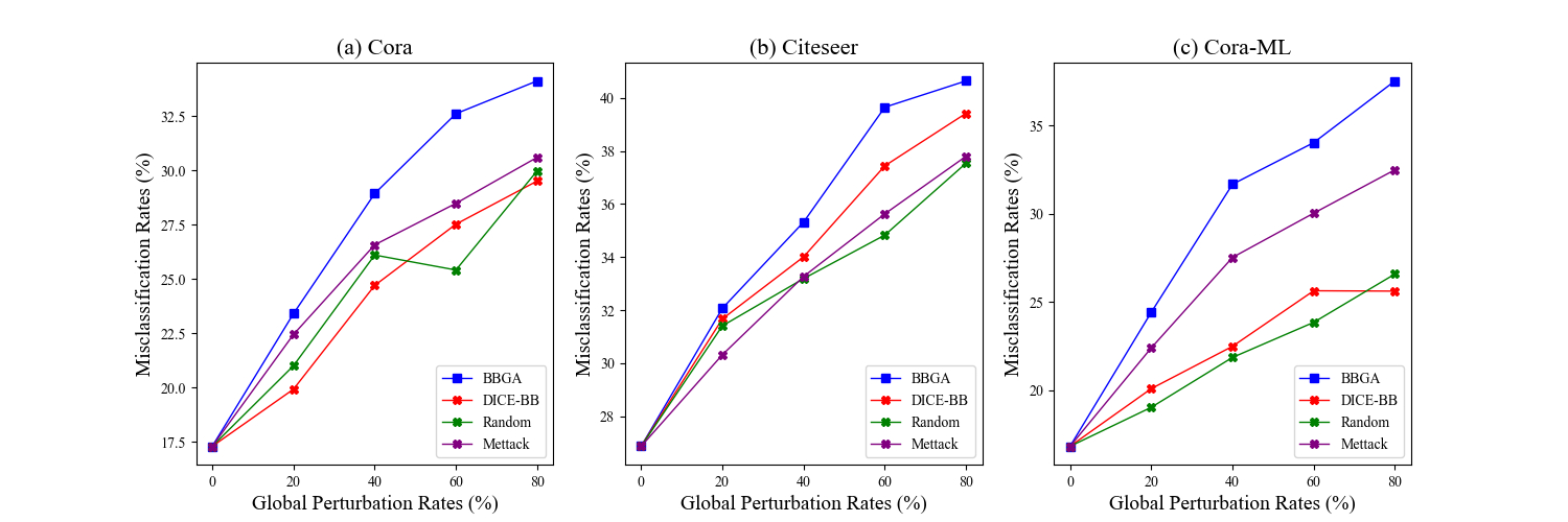
Misclassification rates when attacking against GCN-Jaccard, (a) Cora, (b) Citeseer, (c) Cora-ML.

Figure 3. Misclassification rates when attacking against GCN-Jaccard, (a) Cora, (b) Citeseer, (c) Cora-ML.

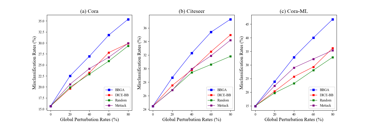
Misclassification rates when attacking against R-GCN, (a) Cora, (b) Citeseer, (c) Cora-ML.

Figure 4. Misclassification rates when attacking against R-GCN, (a) Cora, (b) Citeseer, (c) Cora-ML.

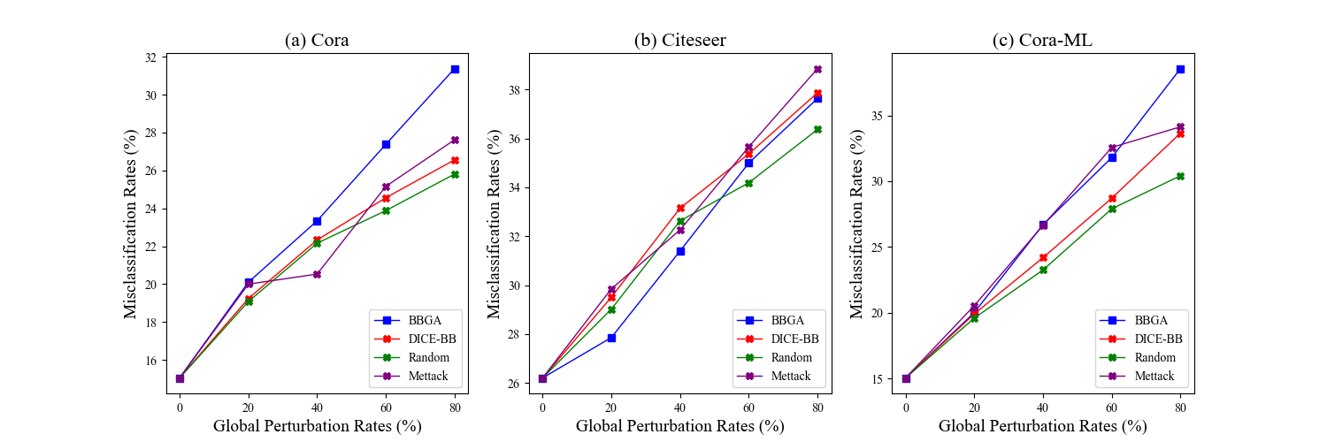
Misclassification rates when attacking against Pro-GNN, (a) Cora, (b) Citeseer, (c) Cora-ML.

Figure 5. Misclassification rates when attacking against Pro-GNN, (a) Cora, (b) Citeseer, (c) Cora-ML.

5.1.4. Parameters and Experimental Settings

We utilize scikit-learn (Pedregosa et al., 2011) for spectral clustering with parameter $\gamma=0.001$. Following (Li et al., 2020) we set $\eta=0.01$. For other hyperparameters, we set $k=5$ and $T=100$.

We conducted our experiments on an Ubuntu 16.04 LTS server with two E5-2650 CPUs and 4 GTX 1080Ti GPUs. Python packages we used include Pytorch 1.5.0, Scikit-Learn 0.23.1, NumPy 1.18.5 and SciPy 1.3.1. Tensorflow 1.15.0 is used in R-GCN defenses.

For each perturbation rate we ran the experiments for 10 times. To verify that our proposed BBGA algorithm is not engaged to any specific training set, we randomly altered the dataset splits with scikit-learn(Pedregosa et al., 2011) each time before the training of the defense algorithms. Following previous works (Zugner and Gunnemann, 2019; Jin et al., 2020b) we choose accuracy rate as the primary evaluation metric.

5.2. Attack Performance

In this subsection, we answer the research question RQ1. Selected results when attacking against the original GCN is reported in Table 3.

We observe from the table that our proposed method outperforms the baselines in all situations when attacking against the original GCN model. Especially, BBGA outperforms the baselines by 20% in several experimental settings.

The performance when attacking against various defend methods are reported in Figures 3, 4 and 5. As shown in the figures, our proposed BBGA algorithms achieves the best misclassification rates in most of the situations. The experiments show that our proposed method is able to achieve a higher misclassification rates when the training set is is not accessible.

5.3. Case Study on Perturbations

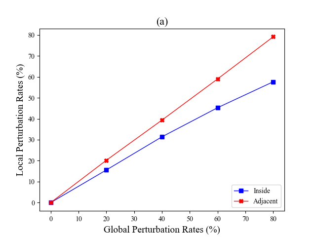
The case study on the distribution of modifications by BBGA algorithm.

Figure 6. The case study on the distribution of modifications by BBGA algorithm.

In this subsection, we answer the research question RQ2 via analysing the perturbations. For a random split of the Cora dataset, we reveal the local perturbation rates in Figure 6. As illustrated in the figure, the perturbations are not biased toward the training set. This demonstrate the evenness of the modifications of our proposed method. It explains the reason why our BBGA algorithm works without accessing the training set.

5.4. Ablation Study and Parameter Analysis

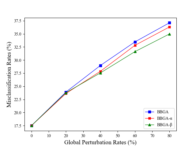
Results of the ablation study

Figure 7. Results of the ablation study.

To answer the research question RQ3, we conducted ablation studies and parameter analysis. For ablation study, we created two variant of our method. BBGA-$\alpha$ removes the filter of low-variance node-pairs in Eq. 12. BBGA-$\beta$ removes the $k$-fold greedy choice procedure and in each step, exactly one partition is chosen randomly to compute the meta-gradient. We took Cora and the GCN model as an example. As revealed in Figure 7, BBGA has the best performance while BBGA-$\beta$ performs the worst. This indicates that both considering multiple partitions and filtering low-variance node-pairs help in increasing the attack performance.

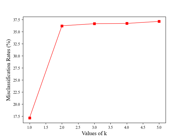
Results of the parameter analysis on k.

Figure 8. Results of the parameter analysis on $k$.

For parameter analysis, we varied the number of partitions $k$. Taking $80\%$ perturbation rates on Cora as an example, it is revealed that the attack performance grow as $k$ increases in general. However, since a larger $k$ implies a longer training time, we suggest to use the hyperparameter $k=5$. The results of the parameter analysis is reported in Figure 8.

6. Conclusion

Previous studies demonstrated that GCNs can be easily fooled by adversarial attacks. However, most existing adversarial attacks requires conditions that are not practical in real-world situations. In this paper, we demonstrate that utilizing training set in adversarial attacks, which is considered to be unrealistic, leads to the lack of robustness. By utilizing pseudo-labels and the $k$-fold greedy strategy, we propose the novel Black-Box Gradient Attack (BBGA) algorithm. Experimental results demonstrate that our proposed algorithm achieves promising performance as a black-box structure-oriented attack. To the best of our knowledge, this is the first gradient-based black-box graph attack and the first non-targeted structure attack that doesn’t require any inquiry. Future directions include further utilization of gradients in black-box scenarios and further investigations in black-box structural attacks.

References

- (1)
- Athalye et al. (2018) Anish Athalye, Nicholas Carlini, and D. Wagner. 2018. Obfuscated Gradients Give a False Sense of Security: Circumventing Defenses to Adversarial Examples. In ICML.
- Carlini and Wagner (2017) N. Carlini and D. Wagner. 2017. Adversarial Examples Are Not Easily Detected: Bypassing Ten Detection Methods. Proceedings of the 10th ACM Workshop on Artificial Intelligence and Security (2017).
- Chen et al. (2020) Liang Chen, J. Li, Jiaying Peng, T. Xie, Zengxu Cao, Kun Xu, X. He, and Z. Zheng. 2020. A Survey of Adversarial Learning on Graphs. ArXiv abs/2003.05730 (2020).
- Dai et al. (2018) Hanjun Dai, Hui Li, Tian Tian, X. Huang, L. Wang, J. Zhu, and L. Song. 2018. Adversarial Attack on Graph Structured Data. In ICML.
- Fricke (2018) S. Fricke. 2018. Semantic Scholar. Journal of the Medical Library Association : JMLA 106 (2018), 145 – 147.
- Geirhos et al. (2019) Robert Geirhos, Patricia Rubisch, Claudio Michaelis, M. Bethge, Felix Wichmann, and W. Brendel. 2019. ImageNet-trained CNNs are biased towards texture; increasing shape bias improves accuracy and robustness. ArXiv abs/1811.12231 (2019).
- Goodfellow et al. (2015) Ian J. Goodfellow, Jonathon Shlens, and Christian Szegedy. 2015. Explaining and Harnessing Adversarial Examples. CoRR abs/1412.6572 (2015).
- Hamilton et al. (2017) William L. Hamilton, Zhitao Ying, and J. Leskovec. 2017. Inductive Representation Learning on Large Graphs. In NIPS.
- Jin et al. (2020a) Wei Jin, Yaxin Li, Han Xu, Yiqi Wang, and Jiliang Tang. 2020a. Adversarial Attacks and Defenses on Graphs: A Review and Empirical Study. ArXiv abs/2003.00653 (2020).
- Jin et al. (2020b) W. Jin, Yao Ma, Xiaorui Liu, Xian-Feng Tang, Suhang Wang, and Jiliang Tang. 2020b. Graph Structure Learning for Robust Graph Neural Networks. Proceedings of the 26th ACM SIGKDD International Conference on Knowledge Discovery & Data Mining (2020).
- Kipf and Welling (2017) Thomas Kipf and M. Welling. 2017. Semi-Supervised Classification with Graph Convolutional Networks. ArXiv abs/1609.02907 (2017).
- Li et al. (2020) Yaxin Li, W. Jin, Han Xu, and Jiliang Tang. 2020. DeepRobust: A PyTorch Library for Adversarial Attacks and Defenses. ArXiv abs/2005.06149 (2020).
- Ma et al. (2020) Jiaqi Ma, Shuangrui Ding, and Q. Mei. 2020. Towards More Practical Adversarial Attacks on Graph Neural Networks. arXiv: Learning (2020).
- Ma et al. (2019) Y. Ma, Suhang Wang, Lingfei Wu, and Jiliang Tang. 2019. Attacking Graph Convolutional Networks via Rewiring. ArXiv abs/1906.03750 (2019).
- Pedregosa et al. (2011) F. Pedregosa, G. Varoquaux, A. Gramfort, V. Michel, B. Thirion, O. Grisel, M. Blondel, P. Prettenhofer, R. Weiss, V. Dubourg, J. Vanderplas, A. Passos, D. Cournapeau, M. Brucher, M. Perrot, and E. Duchesnay. 2011. Scikit-learn: Machine Learning in Python. Journal of Machine Learning Research 12 (2011), 2825–2830.
- Ron and Shamir (2013) D. Ron and A. Shamir. 2013. Quantitative Analysis of the Full Bitcoin Transaction Graph. In Financial Cryptography.
- Scarselli et al. (2009) F. Scarselli, M. Gori, A. Tsoi, M. Hagenbuchner, and G. Monfardini. 2009. The Graph Neural Network Model. IEEE Transactions on Neural Networks 20 (2009), 61–80.
- Sun et al. (2018) Lichao Sun, Yingtong Dou, Carl Yang, Ji Wang, Philip S. Yu, and Bo Li. 2018. Adversarial Attack and Defense on Graph Data: A Survey. arXiv preprint arXiv:1812.10528 (2018).
- Velickovic et al. (2018) Petar Velickovic, Guillem Cucurull, A. Casanova, A. Romero, P. Liò, and Yoshua Bengio. 2018. Graph Attention Networks. ArXiv abs/1710.10903 (2018).
- Wasserman and Faust (2007) S. Wasserman and Katherine Faust. 2007. Social network analysis - methods and applications. In Structural analysis in the social sciences.
- Wu et al. (2019) Huijun Wu, C. Wang, Y. Tyshetskiy, A. Docherty, K. Lu, and L. Zhu. 2019. Adversarial Examples for Graph Data: Deep Insights into Attack and Defense. In IJCAI.
- Xu et al. (2018) Keyulu Xu, C. Li, Yonglong Tian, Tomohiro Sonobe, K. Kawarabayashi, and S. Jegelka. 2018. Representation Learning on Graphs with Jumping Knowledge Networks. In ICML.
- Yan et al. (2009) Donghui Yan, L. Huang, and Michael I. Jordan. 2009. Fast approximate spectral clustering. In KDD.
- Ying et al. (2018) Rex Ying, Ruining He, K. Chen, Pong Eksombatchai, William L. Hamilton, and J. Leskovec. 2018. Graph Convolutional Neural Networks for Web-Scale Recommender Systems. Proceedings of the 24th ACM SIGKDD International Conference on Knowledge Discovery & Data Mining (2018).
- Yuan et al. (2019) Xiaoyong Yuan, Pan He, Qile Zhu, and X. Li. 2019. Adversarial Examples: Attacks and Defenses for Deep Learning. IEEE Transactions on Neural Networks and Learning Systems 30 (2019), 2805–2824.
- Zhou et al. (2018) Jie Zhou, Ganqu Cui, Zhengyan Zhang, Cheng Yang, Zhiyuan Liu, and M. Sun. 2018. Graph Neural Networks: A Review of Methods and Applications. ArXiv abs/1812.08434 (2018).
- Zhu et al. (2019) Dingyuan Zhu, Ziwei Zhang, P. Cui, and Wenwu Zhu. 2019. Robust Graph Convolutional Networks Against Adversarial Attacks. Proceedings of the 25th ACM SIGKDD International Conference on Knowledge Discovery & Data Mining (2019).
- Zügner et al. (2018) Daniel Zügner, Amir Akbarnejad, and Stephan Günnemann. 2018. Adversarial Attacks on Neural Networks for Graph Data. Proceedings of the 24th ACM SIGKDD International Conference on Knowledge Discovery & Data Mining (2018).
- Zugner and Gunnemann (2019) Daniel Zugner and Stephan Gunnemann. 2019. Adversarial Attacks on Graph Neural Networks via Meta Learning.