Spectral solutions of PDEs on networks

Abstract

To solve linear PDEs on metric graphs with standard coupling conditions (continuity and Kirchhoff’s law), we develop and compare a spectral, a second-order finite difference, and a discontinuous Galerkin method. The spectral method yields eigenvalues and eigenvectors of arbitary order with machine precision and converges exponentially. These eigenvectors provide a Fourier-like basis on which to expand the solution; however, more complex coupling conditions require additional research. The discontinuous Galerkin method provides approximations of arbitrary polynomial order; however computing high-order eigenvalues accurately requires the respective eigenvector to be well-resolved. The method allows arbitrary non-Kirchhoff flux conditions and requires special penalty terms at the vertices to enforce continuity of the solutions. For the finite difference method, the standard one-sided second-order finite difference stencil reduces the accuracy of the vertex solution to $O(h^{3/2})$. To preserve overall second-order accuracy, we used ghost cells for each edge. For all three methods we provide the implementation details, their validation, and examples illustrating their performance for the eigenproblem, Poisson equation, and the wave equation.
Keywords: partial differential equations, metric graphs, spectral method, finite difference, discontinuous Galerkin

1 Introduction

Partial differential equations (PDEs) on networks arise in many physical applications such as gas and water networks [Herty et al.(2010)] [Martin et al.(2012)], electromechanical waves in a transmission grid [Kundur(1994)], air traffic control [Work et al.(2008)], and random nanofibre lasers [Gaio et al.(2019)], to name a few. The underlying mathematical model consists of a metric graph: a finite set of vertices connected by arcs (oriented edges) on which a metric is assigned. At the vertices we can have different coupling conditions. The simplest assumes continuity of the field and zero total gradient at the vertices (Kirchhoff’s law). The standard one-dimensional Laplacian together with these boundary conditions results in a generalised Laplacian and associated Helmoltz eigenvalue problem. It can be shown that with these coupling conditions (continuity and Kirchhoff’s law) the problem is self-adjoint, see [Berkolaiko(2017)], yielding real eigenvalues and orthogonal eigenvectors. The eigenvectors form a complete basis of the appropriate set of square integrable functions on the graph.

This spectral framework plays a key role for linear PDEs as we review and apply it in the present article. Using it, the wave equation on a metric graph is treated exactly as the one-dimensional wave equation on a one-dimensional finite interval with simple boundary conditions, see for example [Hildebrand(1976)]. Due to these strong geometrical properties, metric graphs have been studied extensively for the Schrödinger operator (or Helmholtz), see [Gnutzmann et al.(2006)] for a review and the recent book [Noja et al.(2019)] for research on nonlinear PDEs where the self-adjoint framework is not applied. The graph aspect (effect of the large network structure on the PDE solutions) is often overlooked in these studies and remains an undeveloped open area of research. There are few studies of computational methods for PDEs on metric graphs. Exceptions are studies for water and gas networks in the engineering context, see [Martin et al.(2012)] for water networks and [Herty et al.(2010)] for gas networks. Note also our article [Dutykh et al.(2018)] on the sine-Gordon equation. Most methods used there rely on finite difference (FD) spatial discretisations, while a recent study [Arioli & Benzi(2018)] introduced a finite element method (FEM) that is first-order at the vertices with second-order approximation inside the edge. The method was applied to the computations of the quantum graph spectrum, the solution of the elliptic equation, and the time evolution of the diffusion equation.

In this article, we present a systematic procedure to compute eigenvalues and eigenvectors of arbitrary order for a general metric graph and use this spectral framework to compute solutions of linear PDEs on graphs. We compare this spectral method to a second-order FD discretisation using centered finite differences at the inner points of the edges and also second-order approximation to the solution at the vertices. To generalise the finite element approach of [Arioli & Benzi(2018)], we introduce a Discontinuous Galerkin (DG) method of arbitrary polynomial order that allows for exact enforcement of Kirchhoff’s law at the vertices while the continuity of the solution is enforced via penalty term(s) added to the weak formulation. These three methods are compared for the following PDE problems: a generalised Helmholtz, the Poisson equation and a damped wave equation (telegrapher’s equation).

We show that the spectral method is superior for the Helmholtz problem since eigenvalues/eigenvectors of arbitrary order can be computed without resolving the spatial structure of the respective eigenvectors. The FD and the DG methods lose accuracy as the order of the eigenvalue is increased because the spatial structure of the corresponding eigenvector is not resolved. We derive a second-order FD method for the solution at the vertices using ghost points for each edge sharing the same vertex to enforce the Kirchhoff conditions. The standard second-order FD approximations to the derivatives in the Kirchhoff equation result in a reduction of the accuracy of the solutions at the vertices to $O(h^{3/2})$.

The DG of high polynomial order gives very accurate eigenvalues for the resolved modes without any search procedures needed for nonlinear eigenvalue solvers of the spectral method. On the other hand, the solution of the Poisson equation for the DG with common penalty terms to enforce the continuity of the solution is inaccurate due to the large underlying discontinuous solution space unless unresolved modes are filtered out.

For linear evolution PDEs, the spectral components of the solution are fixed by the initial conditions, and the corresponding mode amplitudes decrease exponentially, similar to the one-dimensional linear evolution PDEs on a finite interval, see [Hildebrand(1976)]. Using a one-dimensional Fourier Transform on the initial data of the linear evolution PDEs and on the right hand side of the Poisson equation, an estimate of the modes that are necessary to be resolved for the required accuracy is obtained.

The article is organised as follows. The statement of the problem and a brief review of the background information on metric quantum graphs are provided in Section 2. In Section 3, we describe the numerical spectral method. Section 4 presents the FD and DG methods, emphasising the implementation details. These three methods are applied to the Helmholtz, Poisson, and the telegrapher’s equations, and the results are discussed in Section 5. We conclude with the discussion of the obtained results and ideas for future work in Section 6.

2 Wave equation on the graph

We consider a finite metric graph with $n$ vertices connected by $m$ edges of length $l_{j},\;j=1:m.$ Each edge is parameterised by its length and is oriented arbitrarily from the origin vertex $x=0$ to the end vertex $x=l_{j}$. Following standard graph theory, we call these oriented edges arcs. We recall the definition of the degree of a vertex: it is the number of edges connected to it.

On this graph, we define the vector component wave equation

$$U_{tt}-{\tilde{\Delta}}U=0,$$ (1)

where $U\equiv(u_{1},u_{2},\dots,u_{m})^{T}$. Each component satisfies the one-dimensional wave equation inside the respective arc,

$${u_{j}}_{tt}-{u_{j}}_{xx}=0,~{}~{}~{}j=1,2,\dots,m$$ (2)

In addition, at the vertices the solution should be continuous and also satisfy the Kirchhoff flux conditions at each vertex of degree $d$

$$\sum_{j=1}^{d}\;{u_{j}}_{x}=0,$$ (3)

where $\displaystyle{u_{j}}_{x}$ represent the outgoing fluxes for arc $j$ emanating from the vertex $p$.

Consider equation (1). Since the problem is linear, we can separate time and space and assume a harmonic solution $U(x,t)=e^{ikt}\>V(x)$. We then get a Helmholtz or Schrödinger eigenproblem for $V$ on the graph

$$-{\tilde{\Delta}}V=k^{2}V,$$ (4)

together with the above-mentioned coupling conditions at the vertices and where ${\tilde{\Delta}}$ is the generalised Laplacian, i.e. the standard Laplacian on the arcs together with the coupling conditions at the vertices. This generalised eigenvalue problem admits an inner product obtained from the standard inner product on $L_{2}$ space, see [Solomon(2015)]. We have

$$<f|g>\equiv\sum_{arc~{}~{}j}<f_{j}|g_{j}>,~{}~{}~{}~{}<f_{j}|g_{j}>=\int_{0}^{l_{j}}f_{j}(x)g_{j}(x)dx.$$ (5)

A solution in terms of Fourier harmonics on each branch $j$ of length $l_{j}$ is

$$v_{j}(x)=A_{j}\sin kx+B_{j}\cos kx.$$ (6)

It has been shown that, for the standard coupling conditions used here (continuity and Kirchhoff), the eigenvectors $V^{i}$ form a complete orthogonal basis of the Cartesian product $L_{2}([0,l_{1}])\times L_{2}([0,l_{2}])\dots\times L_{2}([0,l_{m}])$, see [Solomon(2015)]. Writing down the coupling conditions at each vertex, one obtains a homogeneous linear system whose $k$-dependent matrix is singular at the eigenvalues.

Using solution (6) on each arc with unknown coefficients $A_{j}$ and $B_{j}$, the coupling conditions at each vertex yield the homogeneous system

$$M(k)X=0,$$ (7)

of $2m$ equations for the vector of $2m$ unknown arc amplitudes

$$X=(A_{1},B_{1},A_{2},B_{2},\dots A_{m},B_{m})^{T}.$$

The matrix $M(k)$ is singular at the eigenvalues $-k^{2}$. We call these $k$-values resonant frequencies. A practical, robust computational algorithm for the computation of these eigenvalues and eigenvectors is presented in the next section.

For each resonant frequency $k_{q}$, the eigenvectors $V^{q}$ are determined from the null space of matrix $M(k_{q})$. They can then be written as

$$V^{q}=\begin{pmatrix}A^{q}_{1}\sin k_{q}x+B^{q}_{1}\cos k_{q}x\cr A^{q}_{2}\sin k_{q}x+B^{q}_{2}\cos k_{q}x\cr\dots\cr A^{q}_{m}\sin k_{q}x+B^{q}_{m}\cos k_{q}x\cr\end{pmatrix}$$ (8)

They can be normalised using the scalar product defined above. We have

$$\lVert V^{q}\rVert^{2}=<V^{q}V^{q}>=\sum_{j=1}^{m}<V^{q}_{j}V^{q}_{j}>,$$ (9)

where $V^{q}_{j}=A^{q}_{j}\sin k_{q}x+B^{q}_{j}\cos k_{q}x$ and $<V^{q}_{j}V^{q}_{j}>$ is the standard scalar product on $L_{2}([0,l_{j}])$ . This defines a broken L₂ norm or graph norm. The scalar product $<V^{q}_{j}V^{q}_{j}>$ can be computed explicitly

$$<V^{q}_{j}V^{q}_{j}>=\left({A^{q}_{j}}^{2}+{B^{q}_{j}}^{2}\right){l_{j}\over 2}+{\sin{2k_{q}l_{j}}\over 4k_{q}}\left(-{A^{q}_{j}}^{2}+{B^{q}_{j}}^{2}\right)+A^{q}_{j}B^{q}_{j}{1-\cos{2k_{q}l_{j}}\over 2k_{q}}.$$ (10)

Once the eigenvalue problem is solved, one can proceed with the spectral solution of the time-dependent problem, exactly as for the one-dimensional wave equation on an interval. For that, expand the solution of the wave equation on the graph (1) using the eigenvectors,

$$U(x,t)=\sum_{q=1}^{\infty}a_{q}(t)V^{q},$$ (11)

and obtain a simplified description of the dynamics in terms of the amplitudes $a_{q}$.

Let us consider the initial value problem for equation (1) with $U(t=0)=U_{0},~{}~{}U_{t}(t=0)=dU_{0}$. Plugging the expansion (11) into (1) and projecting on the eigenvector $V^{q}$ we get the following amplitude equation

$${d^{2}{a_{q}}\over dt^{2}}+k_{q}^{2}{a_{q}}=0.$$ (12)

The initial conditions for $a_{q}$ are obtained as usual by projecting $U(t=0)$ and $U_{t}(t=0)$ on $V^{q}$. We have

$$a_{q}(t=0)=<U_{0}V^{q}>,~{}~{}{da_{q}\over dt}(t=0)=<dU_{0}~{}V^{q}>.$$ (13)

For example, assuming an initial condition has only support on the first arc,

$$U_{0}=\begin{pmatrix}g(x)\cr 0\cr\vdots\cr 0\cr\end{pmatrix},~{}~{}dU_{0}=\begin{pmatrix}g^{\prime}(x)\cr 0\cr\vdots\cr 0\cr\end{pmatrix},~{}~{}$$ (14)

we get

$$a_{q}(t=0)=<g(x)V^{q}_{1}(x)>,~{}~{}{da_{q}\over dt}(t=0)=<g^{\prime}(x)V^{q}_{1}(x)>.$$ (15)

3 Spectral algorithm

The procedure to compute the eigenvalues and eigenvectors for arbitrary graphs involves the following steps.

1. Form matrix $M(k)$ from the continuity and Kirchhoff linear equations using symbolic manipulations described below.

2. Plot inverse condition number rcond(M(k)) as function of $k$ to estimate graphically the lower bound of the spacing $\Delta k$ between the consecutive values of $k$.

3. Bracket each resonant frequency by splitting the range into smaller sub-intervals.

4. Apply a line minimisation algorithm to the function $\text{rcond}(M(k))$ on each sub-interval to estimate each $k$ within a chosen tolerance.

5. For each resonant frequency, perform a singular value decomposition (SVD) of the matrix $M(k)$ to determine its null space. This will provide the corresponding eigenvector $V$ in (8).

3.1 Generation of the matrix $M(k)$

To generate the matrix $M(k)$, we use the incidence matrix with rows and columns corresponding to the vertices and arcs of the graph. Each column then has two nonzero entries, $1$ and $-1$ reflecting the orientation chosen for this arc.

On each arc, $e_{i}$, for each given resonant frequency $k$, the solution has the form $u_{i}(x)=A_{i}\sin(kx)+B_{i}\cos(kx)$. The continuity condition between arcs $e_{i}$ and $e_{j}$ yields

$$A_{i}\sin(kx_{*})+B_{i}\cos(kx_{*})-\left[A_{j}\sin(kx_{*})+B_{j}\cos(kx_{*})\right]=0$$ (16)

where

$$x_{*}=\begin{cases}0\text{, if arc }e_{r}\text{ is outgoing}\\ l_{r}\text{, if arc }e_{r}\text{ is incoming}\end{cases}$$

To implement the continuity junction condition, our algorithm first finds all unique arc pair combinations at each vertex and saves them to a cell array $C$ (one cell for each vertex containing a list of pairs). For simplicity, the arc with the lowest arc number is fixed and the continuity conditions are written for this arc with every other arc. For a vertex of degree $d$, there will be $d-1$ continuity equations.

For each vertex, the algorithm loops through all of the continuity equations and places respective sines and cosines for each pair $A_{i},B_{i}$ into a row of matrix $M(k)$. In particular, each continuity equation will place the sine term for the $i$th arc in the $(2i-1)$th column, and the cosine term in the $2i$th column schematically shown below,

$$\begin{bmatrix}\sin(kx_{*})&\cos(kx_{*})&-\sin(kx_{*})&-\cos(kx_{*})&\cdots&\vdots\\ \cos(kx_{*})&-\sin(kx_{*})&\cos(kx_{*})&-\sin(kx_{*})&\cdots&\vdots\\ \vdots&\vdots&\vdots&\vdots&\vdots&\vdots\\ \cdots&\cdots&\cdots&\cdots&\cdots&\cdots\end{bmatrix}\begin{bmatrix}A_{1}\\ B_{1}\\ A_{2}\\ B_{2}\\ \vdots\\ \end{bmatrix}=0$$

The Kirchhoff flux vertex condition is implemented at each vertex by summing the derivatives. Note that the $k$ term in front of the sine and cosine will cancel when the sum of the derivatives are set equal to zero and can be omitted. The equation for the flux condition is

$$\sum_{i}A_{i}\cos(kx_{*})-B_{i}\sin(kx_{*})=0.$$ (17)

This equation takes up one row of the matrix for each vertex, thus resulting in $d$ equations for a vertex of degree $d$, with $d-1$ equations from the continuity constraint and one from the flux condition. The result of applying these conditions is the system of equations (7)

Note that languages with symbolic capabilities such as Matlab, Mathematica, etc. have a command that converts linear equations into matrix form using the list of equations and the list of unknowns ($\displaystyle X=(A_{1},B_{1},A_{2},B_{2},\dots A_{m},B_{m})^{T}$) as inputs.

3.2 Finding the resonant $k$s

Once the matrix $M(k)$ is formed, one estimates its inverse condition number $r(k)$,

$$r(k)={1\over\parallel M\parallel_{1}\parallel M^{-1}\parallel_{1}},$$ (18)

using the rcond Matlab function, whose complexity is $O(4m^{2})$, see [Cline et al.(1979)]. In fact, the computation of rcond involves an LU factorisation and its complexity can be estimated using Matlab. We find it to be $O(m^{2})$ for $m<1000$ and $O(m^{3})$ for larger $m$, see Fig. 1.

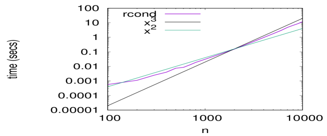
Figure 1: Plot of time in secs as a function of $m$ for rcond.

Note that the resonant frequencies are calculated via the robust inverse condition number estimator rcond(M(k)) instead of a determinant computation that requires arbitrary precision arithmetic for an accurate evaluation. At the resonant $k$s , $M(k)$ is singular and $M^{-1}$ ceases to exist. In practice $\parallel M^{-1}\parallel\to\infty$ so that $r\to 0$.

To find $k^{*}$ such that $r(k^{*})=0$, we implemented a gradient-less line minimisation algorithm, see [Box et al.(1969)]; this is similar to a bisection. This gave $k^{*}$ up to machine precision.

The eigenvector $V^{*}$ associated to the eigenvalue $-{k^{*}}^{2}$ of the generalised Laplacian (4) on the graph can be found using the SVD of $M(k^{*})$

$$M(k^{*})=U\Sigma V^{T}.$$

Since $M(k^{*})$ is singular, it has at least one zero singular value. The column vector of $V$ associated to the zero singular value spans the kernel of $M(k^{*})$.

4 Finite difference and discontinuous Galerkin algorithms

We present here finite difference discretisations and introduce a discontinuous Galerkin approximation.

4.1 Finite difference differentiation matrix on the graph

Here we describe a second-order finite difference method for both the inner arc discretisation and the vertex conditions. The approach can be generalised to higher-order finite differences.

Each arc $e_{i}$ is discretised into $N_{i}+1$ equally-spaced points enumerated from $j=0$ to $j=N_{i}$, with the number of points varying for each edge. $j=0$ and $j=N_{i}$ represent the starting and ending vertex of the edge respectively. Each arc has its own uniform spatial mesh spacing $\Delta x_{i}$. We use a centered, explicit second-order scheme for the second derivative in space,

$$u_{xx}=\frac{u_{j+1,i}-2u_{j,i}+u_{j-1,i}}{\Delta x_{i}^{2}}+{O}\left(\Delta x_{i}^{2}\right)$$ (19)

where $u_{j,i}\approx u(x_{j})$, the solution at $x_{j}$ on a particular edge $e_{i}$ for inner points $j=1,2,\dots,N_{i}-1$.

For the Poisson equation we solve the following FD equation at the inner points

$$\frac{u_{j+1,i}-2u_{j,i}+u_{j-1,i}}{\Delta x_{i}^{2}}=f(x_{j}).$$ (20)

To implement the vertex conditions, we label arcs adjacent to the vertex as $c=1,2,\dots,d$. To enforce the continuity condition we place a node exactly at the vertex and denote the solution value as $u_{0}$. The center vertex $u_{0}$ is shared by each adjacent arc via the continuity condition $u_{c,0}=u_{0}$. To implement the Kirchhoff flux condition, we use a centered, second-order scheme for the first derivative by extending each arc and adding a ghost point next to the vertex at $x=x_{-1,c}$ for each adjacent arc $e_{c}$. The derivative is taken in the outgoing direction from the center vertex. For $j=0$ we have

$$0=\sum_{c=1}^{d}u_{x}(x_{0})=\sum_{c=1}^{d}\frac{u_{1,c}-u_{-1,c}}{2\Delta x_{c}}+{O}(\Delta x_{1}^{2}+\Delta x_{2}^{2}+\cdots+\Delta x_{d}^{2})$$ (21)

Here we say $j=1$ is the point adjacent to the vertex regardless of edge orientation.

We then apply the FD scheme for the PDE. For the Poisson equation we have

$$\frac{u_{1,c}-2u_{0}+u_{-1,c}}{\Delta x_{c}^{2}}=f(x_{0})$$ (22)

This equation can be solved for $u_{-1,c}$ and substituted into the Kirchhoff flux equation to eliminate the ghost point.

$$0=\sum_{c=1}^{d}\frac{u_{1,c}-\left[\Delta x_{c}^{2}f(x_{0})+2u_{0}-u_{1,c}\right]}{2\Delta x_{c}}$$ (23)

This results in the following equation for $u_{0}$ and its neighboring values for placement in the finite difference matrix.

$$2\frac{\sum_{c=1}^{d}\frac{u{1,c}}{\Delta x_{c}}-u_{0}\sum_{c=1}^{d}\frac{1}{\Delta x_{c}}}{\sum_{c=1}^{d}\Delta x_{c}}=f(x_{0})$$ (24)

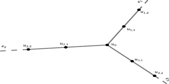
Figure 2: Finite difference discretisation for a vertex of degree 3.

It is important that the orders of the approximation method at the vertices and in the bulk of the arcs be the same. [Arioli & Benzi(2018)] use a piecewise linear basis and enforce continuity of the solution by placing a node at the vertex. This renders the approximation first-order, despite the inner approximation being second order. In our FD scheme, the orders at the vertex and in the bulk of the arcs are the same.

4.2 Discontinuous Galerkin differentiation matrix on the graph

The Discontinuous Galerkin Finite Element Method (DG) is a multi-domain method where the solution is approximated by polynomials on each subdomain with appropriate interface conditions. This allows flexibility in choosing the degree of the polynomials used on the different subdomains and explicitly introduces the interface fluxes in the weak formulation of the problem containing second-order spatial partial derivatives.

In this article, we use orthogonal Legendre polynomials. The Kirchhoff flux conditions are applied explicitly in the weak formulation (natural interface boundary conditions). The continuity of the solution is enforced via a penalty term. In contrast, in the standard finite element approximation introduced in [Arioli & Benzi(2018)], the continuity is enforced by placing a node at each vertex. This resulted in a first-order approximation of the Kirchhoff conditions even though a second-order (piecewise linear) approximation was used inside each arc.

We verify that the error estimate for the Discontinuous Galerkin in the $L_{2}$-norm is $O(h^{p+1})$ where $h$ is the size of the subdomain and $p$ is the degree of the polynomial used on the different subdomains. Note that DG is naturally suitable for an $h-p$ adaptive strategy to determine the most efficient combination between $h$ and $p$ for the problem at hand.

We illustrate the implementation of the DG for the quantum graph eigenvalue problem. Each arc is split into its own number of intervals, $[x_{j},x_{j+1}]$, and equation

$$u_{xx}=-k^{2}u$$ (25)

is rewritten in a weak form for numerical approximation $u(x)$ using test function $\phi(x)$

$$\int\limits_{x_{j}}^{x_{j+1}}u_{xx}\phi\;{\rm d}x=-k^{2}\int\limits_{x_{j}}^{x_{j+1}}u_{x}\phi\;{\rm d}x.$$ (26)

The second derivative term is rewritten in equivalent ultra-weak form after applying three integration by parts, see [Chen et al.(2019)],

$$\int\limits_{x_{j}}^{x_{j+1}}u_{xx}\phi\;{\rm d}x=-\int\limits_{x_{j}}^{x_{j+1}}u_{x}\phi_{x}\;{\rm d}x+u_{x}\phi\Bigr{|}_{x_{j}}^{x_{j+1}}+(u-u)\phi_{x}\Bigr{|}_{x_{j}}^{x_{j+1}}.$$ (27)

Among numerous penalty methods for the DG method applied to the second-order spacial derivatives [Chen et al.(2019)], we chose the following approach that can be generalised to the graph vertices to enforce continuity there, and also allows for applying both Kirchhoff and non-Kirchhoff scattering flux conditions at the vertices to be explored in the future.

For the inner intervals (endpoints do not include the vertices) the communication between neighboring intervals is introduced through both boundary terms that are evaluated as follows,

$${\widetilde{u}}_{x}\phi\Bigr{|}_{x_{j}}^{x_{j+1}}+(u-{\widehat{u}})\phi_{x}\Bigr{|}_{x_{j}}^{x_{j+1}},$$ (28)

where the $\widehat{u}$ denotes the arithmetic average across the jumps, while ${\widetilde{u}}_{x}$ has an additional penalty term to enforce continuity of the solution across the jumps of the DG piecewise polynomial basis, e.g. at $x_{j}$

$$\widehat{u}=\frac{u_{j}^{-}+u_{j}^{+}}{2},\qquad{\widetilde{u}}_{x}=\frac{{u_{x}}_{j}^{-}+{u_{x}}_{j}^{+}}{2}-\frac{\gamma\;(u_{j}^{+}-u_{j}^{-})}{\Delta x_{j}},$$ (29)

where $\Delta x_{j}$ is the length the interval $[x_{j},x_{j+1}]$ and the rest of the variables are evaluated using their respective left and right values on the interval $[x_{j},x_{j+1}]$. The constant $\gamma$ was set experimentally to $\gamma=200(p+1)^{2}$, see [Chen et al.(2019)], where $p$ is the degree of the polynomial used in the DG approximation.

For the intervals that have a vertex as one of their endpoints, $\widehat{u}$ is computed as an arithmetic average over all edge values that share the common vertex. Note, that the term containing $(u-\widehat{u})$ is an additional a penalty term to enforce the continuity condition at the interval interfaces (and may omitted), but it is the only penalty term that is used at the vertices to enforce the continuity of the solution there. Without it, the numerical solution is convergent, but the limiting function is discontinuous at the vertices, and thus it is not a solution of the original Poisson problem with the stated vertex conditions (continuity plus Kirchhoff constraints).

The flux value $u_{x}^{(j)}$ at the $j$th vertex is computed from Kirchhoff’s condition,

$$u_{x}^{(j)}=-\sum\limits_{\text{all}\;m\neq j}u_{x}^{(m)}\;.$$ (30)

Therefore, DG allows one to apply exact Kirchhoff flux conditions in the problem formulation whereas the continuity condition is enforced via the penalty term.

Finally, for each arc and each interval on these arcs $\displaystyle[x_{j},x_{j+1}]$ of size $\displaystyle\Delta x_{j}=x_{j+1}-x_{j}$, the numerical solution $u(x)$ is represented as

$$u(x)=\sum\limits_{m=0}^{p}c_{m}\tilde{P}_{m}(x),$$ (31)

where $\displaystyle\tilde{P}_{m}(x)=P_{m}\Big{(}-1+2(x-x_{j})/\Delta x_{j}\Big{)}$, where $P_{m}(x)$ are standard Legendre polynomials orthogonal on the interval $x\in[-1,1]$,

$$\int\limits_{x_{j}}^{x_{j+1}}\tilde{P}_{m}(x)\tilde{P}_{k}(x)\;{\rm d}x=\frac{\Delta x_{j}}{(2m+1)}\;\delta_{mk}.$$ (32)

The degree $p$ of the polynomials on each arc and each interval within it may vary arbitrarily as communication between neighbouring polynomials is achieved via interface or vertex values that can be easily evaluated using the above formulas regardless of the polynomial degrees involved.

On the interval $[x_{j},x_{j+1}]$ we also use the following properties to compute the interface values of the Legendre polynomials,

$$\tilde{P}_{m}(x_{j+1})=1,\;\;\;\tilde{P}_{m}(x_{j})=(-1)^{m},\\$$ (33)

$$\tilde{P}^{\prime}_{m}(x_{j+1})=\frac{m(m+1)}{\Delta x_{j}},\;\;\;\;\tilde{P}^{\prime}_{m}(x_{j})=(-1)^{m+1}\;\tilde{P}^{\prime}_{m}(x_{j+1}),$$ (34)

as well as precompute each inner product on the standard $[-1,1]$ interval using identity relating it to the arbitrary interval $[x_{j},x_{j+1}]$,

$$\int\limits_{x_{j}}^{x_{j+1}}\tilde{P}_{m}^{\prime}(x)\tilde{P}_{l}^{\prime}(x){\rm d}x=\frac{2}{\Delta x_{j}}\int\limits_{-1}^{1}P_{m}^{\prime}(x)P_{l}^{\prime}(x)\;{\rm d}x.$$ (35)

The test function for the DG method on each interval $[x_{j},x_{j+1}]$ are $\tilde{P}_{l}(x)$, $l=0,1,2,\dots,p.$

In the following section we compare the theoretical and numerical error estimates for the FD and DG methods.

5 Numerical results

Here we validate an implementation of the numerical methods described in the previous sections for the eigenvalue problem, the steady-Poisson equation and the time-dependent wave equation. We choose three model graphs: a pumpkin graph [Berkolaiko(2017)], a graph obtained from an electrical grid model, and a graph coming from a laser based on a random network of optical fibres.

The first graph is a simple three arc pumpkin graph shown in Fig. 3 with arc lengths $l_{1}=\sqrt{2},~{}l_{2}=\sqrt{3},~{}~{}l_{3}=\sqrt{5}$,

Figure 3: A three arc pumpkin graph.

A second graph is a 14-vertex graph G14 adapted from the IEEE benchmark test, see [University of Illinois Information Trust Institute(2021)]. It is shown in Fig. 4.

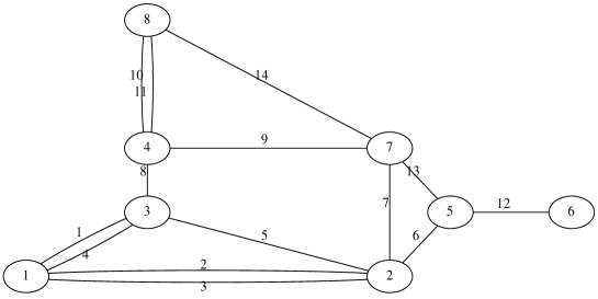
Figure 4: The 14-vertex graph

The lengths $l_{i}$, $i=1,\dots,14$ are given in the table below.

$l_{1}$	$l_{2}$	$l_{3}$	$l_{4}$	$l_{5}$
11.91371443	7.08276253	6	2.236067977	4.123105626
$l_{6}$	$l_{7}$	$l_{8}$	$l_{9}$	$l_{10}$
1.414213562	2	1	4.7169892	4.472135955
$l_{11}$	$l_{12}$	$l_{13}$	$l_{14}$
2	2	1.414213562	4.472135955

Table 1: The lengths $l_{i}$ for the graph G14.

We also consider an example of a random graph, a Buffon’s needle graph with 165 arcs and 104 vertices, see Fig. 5. We generated a version of Buffon’s needle graph using a code developed by Michele Gaio, [Gaio et al.(2019)]. To create the graph, $n$ random points are uniformly generated on a square with diagonal $L$. A straight line segment (needle) with random angle and length is drawn from each point. The needles are all given the same diameter $D$. The intersections of line segments become the vertices of the graph. If two vertices are within a distance $r=\left(\frac{12D}{L}\right)^{2}$ of each other, they are combined into a single vertex. The arcs of the graph are the lengths along the needles connecting the vertices. The resulting graph appears as a series of scattered needles. By construction, most vertices are degree four, with on average 15% of vertices of degree six.

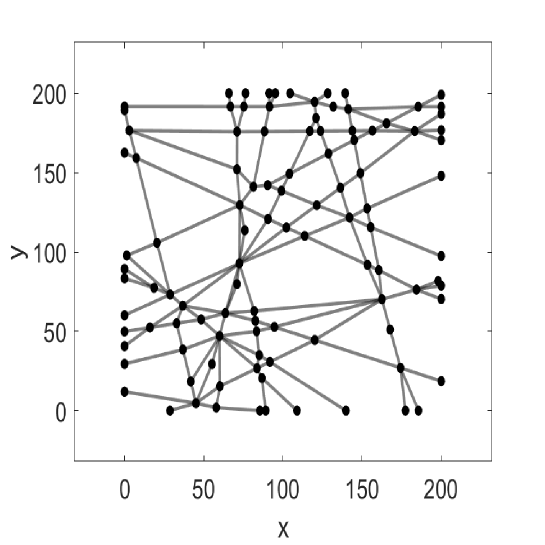
Figure 5: Buffon’s needle graph.

5.1 Eigenvalues and Weyl’s law

To illustrate the spectral algorithm for finding eigenvalues using exact eigenvectors given by Fourier modes of equation (6), we outline the steps involved on a pumpkin graph (Fig. 3). Enforcing continuity and Kirhchoff’s law at vertices $1$ and $2$, respectively, gives

$$B_{1}=B_{2}=B_{3},$$ (36)

$$A_{1}+A_{2}+A_{3}=0,$$ (37)

$$A_{1}s_{1}+B_{1}c_{1}=A_{2}s_{2}+B_{2}c_{2}=A_{3}s_{3}+B_{3}c_{3},$$ (38)

$$A_{1}c_{1}-B_{1}s_{1}+A_{2}c_{2}-B_{2}s_{2}+A_{3}c_{3}-B_{3}s_{3}=0,$$ (39)

where $s_{1}=\sin kl_{1},c_{1}=\cos kl_{1}$, etc. This yields the following linear system

$$M(k)\begin{pmatrix}A_{1}\cr B_{1}\cr A_{2}\cr B_{2}\cr A_{3}\cr B_{3}\end{pmatrix}=\begin{pmatrix}0\cr 0\cr 0\cr 0\cr 0\cr 0\end{pmatrix}.$$ (40)

where the matrix $M(k)$ is

$$M(k)\equiv\begin{pmatrix}.&1&.&-1&.&.\cr.&1&.&.&.&-1\cr 1&.&1&.&1&.\cr s_{1}&c_{1}&-s_{2}&-c_{2}&.&.\cr s_{1}&c_{1}&.&.&-s_{3}&-c_{3}\cr c_{1}&-s_{1}&c_{2}&-s_{2}&c_{3}&-s_{3}\end{pmatrix}$$ (41)

Setting the inverse condition number of the matrix $M(k)$ to $0$, we obtain the equations for the resonant frequencies $k$, and then compute the eigenvalues using relation $\lambda=-k^{2}$. The first three nonzero eigenvalues and corresponding eigenvectors $V^{q}=(v^{q}_{1},v^{q}_{2},v^{q}_{3})^{T}$ are given in the Table 2.

$q$	$-k_{q}^{2}$	$A^{q}_{1}~{}/~{}B^{q}_{1}$	$A^{q}_{2}~{}/~{}B^{q}_{2}$	$A^{q}_{3}~{}/~{}B^{q}_{3}$
1	-2.395998	-0.24204	-0.53262	0.77466
		-0.12486	-0.12486	-0.12486
2	-3.057162	0.20191	0.03291	-0.23481
		-0.58105	-0.58105	-0.58105
3	-4.067077	0.85001	-0.69799	-0.15202
		0.123927	0.123927	0.123927

Table 2: First three nonzero eigenvalues and eigenvector components for the pumpkin graph.

To compute the resonant frequencies we estimate the minimum spacing graphically and split the range of $k$ into intervals of about $1/10$ of the estimated minimum spacing. Each minimum of $r(k)$ is found using a Brent-like minimisation algorithm that we implemented, e.g. a secant method with bracketing see [Box et al.(1969)] for example. A more efficient algorithm that we did not pursue here would be to use the sawtooth nature of the rcond(M(k)) functions as shown in Fig. 6 and alternate between min and max search algorithms to find peak and valley values only.

To illustrate the practicality and robustness of our algorithm, we show rcond(k) for $k\in[568,577]$ in Fig. 6. Such high-order eigenvalues and eigenvectors can be computed easily with the spectral method as opposed to FD or DG, for which the spatial structure of the eigenvectors need to be resolved. The spacing between the resonant $k$s is fairly regular except at exceptional locations, such as the one shown in Fig. 6 where the $k$ in $[572,574]$ need a finer bracketing, see right panel of the figure. Nevertheless, the line minimisation yields the estimates of $k$ at machine precision

$$573.14678431204834,~{}~{}573.17977474169390,~{}~{}573.20510976082187~{}.$$

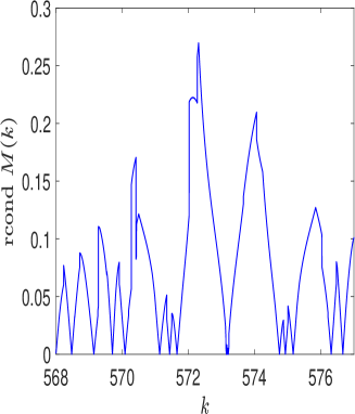
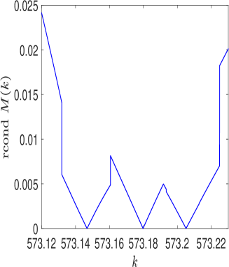
Figure 6: Pumpkin graph: plot of rcond(k) for $k\in[568,577]$ (left panel), blow-up of the plot (right panel).

Weyl’s law

The eigenvalues $k^{2}$ of the generalised Laplacian (4) of graphs follow Weyl’s law [Berkolaiko(2017)]. For a positive real number $q$, the number of eigenvalues $k^{2}\leq q^{2}$ is given by Weyl’s estimate

$$qL/\pi,$$ (42)

where $L$ is the sum of the lengths of all the arcs of the graph. In addition, the distribution of eigenvalues is also bounded from above and below by two lines with the same slope

$$qL/\pi-\left|E\right|\leq\;\#\{k\big{|}k^{2}\leq q^{2}\}\;\leq qL/\pi+\left|V\right|,$$ (43)

as illustrated in Fig. 7. Here, $\left|E\right|$ represents the number of arcs, and $\left|V\right|$ represents the number of vertices.

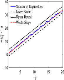
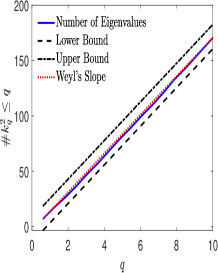
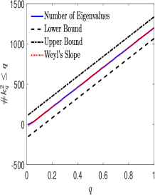
Figure 7: Distribution of the resonant frequencies vs Weyl’ law estimates for the Pumpkin (left), G14 (middle) and Buffon’s (right) graphs.

As seen in Fig. 7, the distribution of eigenvalues follows Weyl’s law with $L=5$ (pumpkin graph), 40 (G14) and 2700 (Buffon).

Since root-finding accuracy is independent of the $k$-value for the spectral algorithm, it is superior to both FD and DG methods, as their accuracy depends on spatially resolving the eigenvector. For example, on the pumpkin graph, for $\displaystyle k=573.18$ shown in Fig. 6, one has to resolve the wavelength $10^{-3}$. This would require a spatial step $\Delta x\approx 10^{-12}$ for the error to reach machine precision, see equation 44 below. For DG with 5th-order polynomial, the sub-intervals should be about $h=10^{-3}$ for the error to reach machine precision. For fixed mesh size, the consecutive eigenvalues become less and less precise for both FD and DG methods, as shown in Fig. 8 for the first 30 resonant frequencies for the pumpkin graph. Fig. 8 shows the errors in the eigenvalues for the FD and DG methods, using the spectral estimation as an exact value.

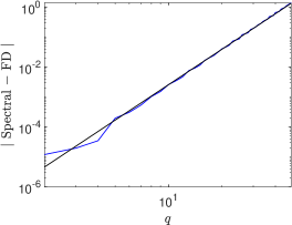
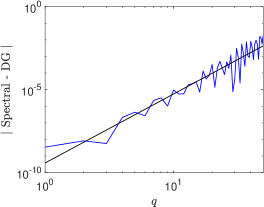
Figure 8: Absolute errors for the $q$th eigenvalue vs $q$ for the FD (left panel) and the DG (right panel) algorithms.

Note the linear scalings of the absolute errors. For the FD, we have

$$\log_{10}({\rm abs.~{}error})=3.93\log_{10}(q)-6.52$$ (44)

The eigenvalues of the tridiagonal matrix that approximates the second derivative are

$$-(4/\Delta x^{2})\sin(\pi k\Delta x/2)^{2}\approx-k^{2}\pi^{2}+O(k^{4}\Delta x^{2})$$

in a Taylor expansion around $\Delta x=0$. This explains the scaling $k^{4}$ observed for the error of the FD method.

For the DG, the equation of the line is

$$\log_{10}({\rm abs.~{}error})=4.15\log_{10}(q)-9.42~{}.$$ (45)

The DG method can be used to estimate the eigenvalues of high-order for the generalised Laplacian (4). Fig. 9 shows the error as a function of $q$. As expected, accuracy decreases as the order of the eigenvalue increases. For $h=0.01$, the error for $q=150$ is $10^{-5}$, and the error reaches $10^{-1}$ for $q=450$.

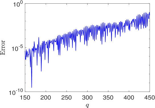
Figure 9: Pumpkin graph: error in DG estimation of eigenvalues of high order, $h=0.01,~{}~{}p=5$.

Since the form of the eigenvectors of the generalised Laplacian (4) are known exactly, the only approximation required is to find the real zeros of a scalar real function. This can be done for thousands of eigenvalues within machine precision. In contrast, for the FD and DG methods, computing the eigenvalues accurately requires the accurate resolution of the corresponding eigenvectors. This is much more computationally expensive, even with the DG method that allows an arbitrary polynomial order of accuracy, $O(h^{p+1})$, where $h$ is the interval size in splitting the arcs and $p$ is the smallest polynomial order used for approximating the solution on each interval.

In the next two sections, we discuss solutions of the Poisson and wave equations using the three methods under consideration: spectral Fourier, FD, and DG methods.

5.2 Poisson equation

Consider Poisson’s equation

$$\hat{\Delta}U=F$$ (46)

where $\hat{\Delta}$ stands for the generalised Laplacian on the graph (4).

Using the spectral decomposition, expand both $U$ and $F$ in terms of the eigenvectors $V^{q}$ of the equation (4), $\displaystyle\Delta V^{q}=-k_{q}^{2}V^{q}$,

$$U=\sum_{q=0}^{\infty}\alpha_{q}V^{q},~{}~{}~{}~{}F=\sum_{q=0}^{\infty}\beta_{q}V^{q}.$$ (47)

Since 0 is an eigenvalue of the Laplacian with corresponding constant eigenvector, the compatibility condition (Fredholm alternative) requires $\beta_{0}=0$. The rest of the unknown coefficients $\alpha_{q}$ are obtained by projecting onto the eigenvectors $V^{q}$ using the scalar product (9)

$$\alpha_{q}=-{\beta_{q}\over k_{q}^{2}},\;\;q=1,2,3,\dots$$ (48)

Since the eigenfunctions are orthogonal, Bessel’s identity allow one to measure the error due to series truncation in terms of the decay of the expansion coefficients.

In Fig. 11 we show the accuracy of the solution for the pumpkin graph in terms of the accuracy of the function $f$ expansion, $\log 10(\beta_{q})$ (left) and $\log 10(\alpha_{q})$ (right), respectively, in terms of the number of terms in partial sums in (47). The initial condition is a derivative of the Gaussian on arc 2 (that has zero average) and zero on the other arcs.

$$g(x)=-2{x-x_{0}\over s^{2}}\exp(-{(x-x_{0})^{2}\over s^{2}}),$$ (49)

with $x_{0}=0.865~{}~{}s=0.15$.

The problem has an exact solution, up to an arbitrary constant

$$u_{1}(x)=-0.04431134627263788525+0.06267946415920350157x,$$ (50)

$$u_{2}(x)=0.08862269254527577050-0.10232143801160161859x+{3\sqrt{\pi}\over 40}{\rm erf}({200x-173\over 30}),$$ (51)

$$u_{3}(x)=-0.04431134627263788525+0.03964197385239476854x.$$ (52)

The consistency of the three numerical methods with the exact solution is shown in Fig. 10. The arbitrary constant is determined by a least square fit of the difference between the exact and the numerical solution.

Here we solve (46) for the pumpkin graph with $\Delta x=0.01$ and a right hand side $F$ given by (49) placed on arc 2 with length = $\sqrt{3}$ and $0$ on the other edges. The parameters are $x_{0}=0.865$ and $s=0.15$.

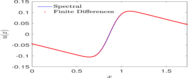
Figure 10: Solutions of Poisson’s equation (46) with a right hand side given by (49) in arc 2 and zero in the other arcs.

The convergence of the spectral amplitudes $\alpha_{q}$ and $\beta_{q}$ vs the number of modes $q$ is shown in Fig. 11.

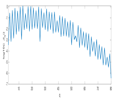
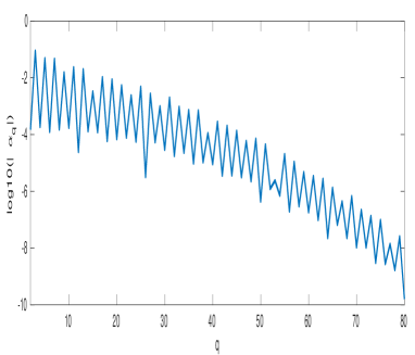
Figure 11: Base 10 logarithms of the amplitudes $\beta_{q}$ (left) and $\alpha_{q}$ (right) for the function $g$ given as (49) on arc 2 of the pumpkin graph.

The semilog plot shows that the coefficients $\beta_{q}$ and $\alpha_{q}$ decay exponentially with $q$ (spectral accuracy), as expected for the Fourier expansion of analytical functions. For example, an expansion with fifty modes allows one to reach a solution with accuracy (absolute error) of $10^{-8}$.

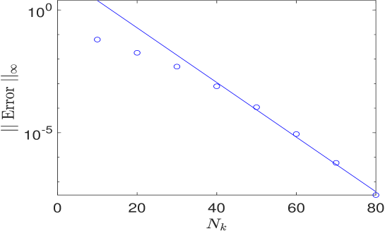
Figure 12: $L_{\infty}$ norm of the difference between the spectral solution and the exact solution (50) as a function of the number of modes $N_{k}$ used in the expansion.

To confirm these results, we plot in Fig. 12 in log-linear scale the $L_{\infty}$ norm of the difference between the spectral solution (48) and the exact solution (50) as a function of $N_{k}$ the number of modes used in the expansion. As expected, we observe an exponential decay of the error.

For both the FD and DG methods, solving the Poisson equation (46) reduces to solving the linear system $\displaystyle A\tilde{u}=b$,where $A$ represent the discrete Laplacian approximated using the FD or DG method and where $b$ represents the strong and weak approximations of the function $F$, respectively, as described in the previous section. The $\tilde{u}$ represents the unknown discrete values of $u$ or the expansion coefficients in Legendre polynomials for the DG method.

The matrix $A$ is singular due to the zero eigenvalue corresponding to a constant eigenvector and a pseudo-inverse is used to find the solution without the arbitrary constant belonging to the null space of A. We rewrite $A$ in its reduced SVD form, $A=\hat{U}\hat{\Sigma}V^{T}$ and solve for $u$,

$$u=A^{\dagger}F,$$ (53)

where $A^{\dagger}=V\hat{\Sigma}^{-1}\hat{U}^{T}$.

The error for the FD method is shown in Fig. 13.

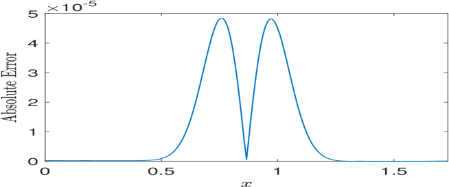
Figure 13: Errors of the FD method for the solution of Poisson’s equation (46) with a right hand side given by (49) in arc 2 and zero in the other arcs.

To conclude on the FD, we show in Fig. 14 the error for the standard vertex approximation used by [Arioli & Benzi(2018)] and the method we used, i.e. centered FD with ghost points. Clearly the former is first order while the latter is second order.

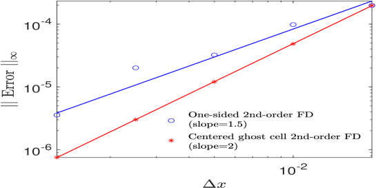
Figure 14: Plot of the error vs. $\Delta x$ for two approximations of the Kirchoff vertex condition: centered FD with ghost points 2nd order (red online) and one-sided FD approximation (blue online)

The DG approximation converges at the optimal convergence rate $O(h^{p+1})$ as illustrated in table below that provides the errors in $L_{\infty}$-norm. The error is maximal near the inflection point of the solution on the second edge. It is lower by an order of magnitude or two away from the inflection point and on the other two edges. The condition number of the matrix grows exponentially with the size $n$ of the matrix and the error saturates for $p=5$ and $h=0.01$, see Table 3. At this point, the SVD loses precision, as confirmed by the exact computation in rational arithmetic using Mathematica, which gives an error for $p=5,h=0.01$ of $4.9~{}10^{-13}$ instead of $3.3~{}10^{-10}$. To avoid this loss of accuracy in finite precision, one could use a preconditioner as suggested by [Arioli & Benzi(2018)].

	0.1	0.01
1	$7.0~{}10^{-3}$	$6.0~{}10^{-5}$
2	$6.9~{}10^{-4}$	$7.0~{}10^{-7}$
3	$5.7~{}10^{-5}$	$5.0~{}10^{-9}$
4	$6.0~{}10^{-6}$	$8.5~{}10^{-11}$
5	$3.3~{}10^{-7}$	$3.3~{}10^{-10}$

(a) $O(h^{p+1})$ numerical error

p	n	$cond(A)_{2}$	n	$cond(A)_{2}$
1	106	$1.3~{}10^{5}$	1078	$1.3~{}10^{7}$
2	159	$5.9~{}10^{5}$	1617	$6.0~{}10^{7}$
3	212	$1.0~{}10^{6}$	2156	$1.0~{}10^{8}$
4	265	$2.4~{}10^{6}$	2695	$2.5~{}10^{8}$
5	318	$3.5~{}10^{6}$	3234	$6.6~{}10^{8}$

(b) $cond(A)_{2}$ vs degree $p$ of polynomial

Table 3: DG solution errors in $L_{\infty}$-norm and condition number in $L_{2}$-norm for the matrix $A_{n\times n}$.

5.3 Wave equation

Here, we consider a telegrapher’s equation that generalises both the wave and heat equations by adding dispersive and damping terms when $\gamma\neq 0$ and $\beta\neq 0$, respectively,

$$\alpha U_{tt}+\beta U_{t}-{\tilde{\Delta}}U+\gamma u=0.$$ (54)

The eigenvectors $V^{q}$ of the generalised Laplacian form a complete basis of eigenvectors of $L^{2}(\Omega)$. It is then natural to expand $U$ as

$$U=\sum_{q}\alpha_{q}(t)V^{q}.$$

Substituting the expansion into (54) we obtain the following evolution equation for the coefficients $\alpha_{q}$

$$\alpha{\ddot{\alpha}_{q}}+\beta{\dot{\alpha}_{q}}+k_{q}^{2}\alpha_{q}+\gamma\alpha_{q}=0.$$ (55)

Given the initial condition this equation can be solved exactly for each Fourier amplitude $\alpha(t)$.

Note that when $\alpha=0$, equation (54) reduces to the generalised heat equation on the metric graph. The evolution of the coefficients $\alpha_{q}$ is given by

$${\dot{\alpha}_{q}}+k_{q}^{2}\alpha_{q}+\gamma\alpha_{q}=0,$$ (56)

where we chose $\beta=1$ for simplicity. The solution of (56) is

$$\alpha_{q}(t)=\alpha_{q}(0)\exp\left[{-(k_{q}^{2}+\gamma)t}\right].$$ (57)

Exactly as for the one-dimensional heat equation, the large $k_{q}$ coefficients decay fast and only $\alpha_{q}$ for the smallest $k_{q}$ can be observed as time evolves. It is then particularly important to estimate this first eigenvalue, the so-called spectral gap [Berkolaiko(2017)]. It could explain the oscillations observed in gas networks, see [Chertkov et al.(2015)].

Both FD and DG methods applied directly to (54) would require one to solve the ODEs for the unknown solution values and expansion coefficients $c_{m}(t)$ in terms of the Legendre polynomials (31) of the form

$$M\ddot{C}(t)+L\>\dot{C}(t)+K\>C(t)+\Gamma\>C(t)=0.$$ (58)

Below we illustrate the behavior of the total energy over time for the wave equation on the pumpkin graph. On a network with $m$ arcs, the energy $E$ is given by

$$E=\sum_{i=1}^{m}\int_{0}^{l_{i}}\frac{1}{2}\left(\left(\frac{\partial u}{dt}\right)^{2}+\left(\frac{\partial u}{dx}\right)^{2}\right)\,dx$$ (59)

for solution $u(x,t)$ and is constant in time. For the pumpkin graph, the energy of the second mode is computed to machine precision as $E_{2}=1.211142452041264$. The energy of the FD approximation to the solution was computed using centered second-order approximations to the derivatives for the inner points and one-sided second-order approximations to the spatial derivative for the vertices. The integrals are approximated with the trapezoid rule. The time evolution of $E$ is shown in Fig. 15. Though the energy for the exact solution is constant, the energy of the FD solution oscillates around a constant state, as the vertices produce small oscillations in time. These decay as $\Delta x^{2}$ with refinement.

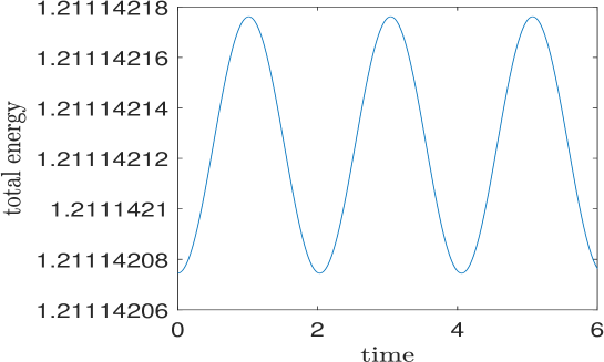
Figure 15: Pumpkin graph: total energy for the wave equation using the second eigenvector $V^{2}$ ($k_{2}=1.5479012370538900$) as initial condition. The time and space steps are $\Delta t=5\times 10^{-4}$ and $\Delta x=6.25\times 10^{-4}$ .

5.4 Discussion

An important issue when solving a PDE on a metric graph is the choice of the number of modes (eigenvectors) for the representation of the initial condition. Once the modes are fixed, the (linear) PDE solution will evolve according to them. No new modes will be excited.

The number of modes necessary to resolve the initial condition depends on its length scales. To illustrate this issue, consider a Gaussian initial condition

$$f(x)=\exp(-{(x-x_{0})^{2}\over s^{2}}),$$ (60)

on arc $a$, of length $l_{a}$ with $x_{0}=l_{a}/2$ and $s=l_{a}/10$. The other arcs are set to zero. We expand the initial condition as in equation (47).

Fig. 16 shows the logarithms of the mode amplitudes $\alpha_{q}$ vs. $k_{q}$ for the G14 graph for two Gaussian initial conditions on arcs 1 ($l_{1}=11.91$) and 6 ($l_{6}=\sqrt{2}$). Clearly, the former is resolved as the amplitudes $|\alpha_{q}|$ decay. On the contrary, for the initial condition set on arc 6, the $|\alpha_{q}|$s do not decay, so many more modes are needed.

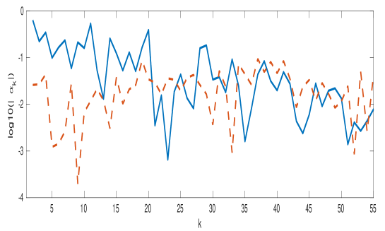
Figure 16: Logarithms of the mode amplitudes $\alpha_{q}$ vs. $k_{q}$ for the initial condition (60) set on arc 1 ($l_{1}=11.91$) continuous line (blue) and arc 6 ($l_{6}=\sqrt{2}$) in dashed line (red). The parameters are $x_{0}=l/2$ and $s=l/10$.

This is confirmed by a one-dimensional Fourier analysis of the two Gaussians shown in Fig. 17. The Gaussian on arc 1 extends up to $k=5$ while the one on arc 6 extends up to $k=25$.

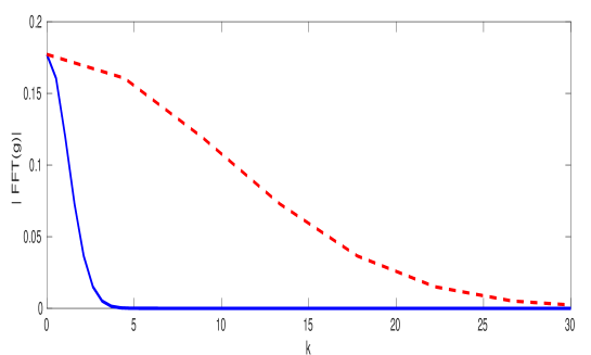
Figure 17: Modulus of the one dimensional Fourier transform of the Gaussians (60) in arc 1 in continuous line (blue) and 6 in dashed line (red).

This simple analysis shows that a one-dimensional Fourier analysis provides an estimate of the number of modes needed to resolve the initial condition. For an inhomogeneous network such as G14, the number of modes needed can be very large if the initial condition is concentrated on a small arc.

6 Conclusion

In this article we developed and compared a spectral, a second-order finite difference and a discontinuous Galerkin method for solving linear PDEs on a metric graph with continuity and Kirchhoff vertex conditions. The spectral approach relies on a practical and robust algorithm for estimating the eigenvalues and eigenvectors of the generalised Laplacian on a metric graph. It builds the matrix $M(k)$ and finds the singular $k$s using line optimisation on the rcond inverse condition number estimate and yields eigenvalues and eigenvectors of arbitrary order to machine precision. We used this spectral formalism to solve a generalised Helmholtz problem, the Poisson equation, and the telegrapher’s equation.

The FD method guarantees continuity of the solution as the computational node is placed at the vertices connecting the arcs. To achieve the second-order accuracy at the vertices, we placed a ghost grid point for each vertex. The standard second-order one-sided difference approximation to the fluxes in Kirchhoff’s law reduced the accuracy of the solution at the node to the first-order as did the use of weighted arithmetic average of the nearby values.

The DG method allows us to include exact Kirchhoff and non-Kirchhoff flux conditions, but the continuity of the solution at the interval interfaces and the vertices requires the introduction of penalty terms. This method provides arbitrary polynomial accuracy for spatial approximations, but the condition number of the stiffness matrix grows exponentially, and for large problems it requires the selection of an appropriate preconditioner.

The spectral method converges exponentially with the number of modes. It is superior for computing eigenvalues/eigenvectors of the generalised Laplacian of arbitrary order, whereas the other two methods require the spatial resolution of highly oscillatory eigenvectors in such cases. In addition, the spectral approach provides a very simple formalism for linear PDEs on graphs, exactly as for a one-dimensional linear PDE on an interval. One first computes the spectral coefficients of the right hand side of the Poisson problem or the initial conditions for the telegrapher’s equation. Then the solution is written explicitly in terms of these modes. Since the evolution problem is linear, each mode evolves separately, and no new modes appear. On the other hand, non-Kirchhoff vertex conditions, e.g. when the flux at each arc depends on the fluxes at the other arcs, result in an overdetermined system and require special consideration to enforce continuity. In this situation, the generalised Laplacian is not self-adjoint [Berkolaiko(2017)] so the eigenvalues may become complex and the eigenvectors not orthogonal. This makes the spectral method much more complicated.

Finally note that for some nonlinear problems, the spectral method can be used as part of the time-split algorithms providing spectrally accurate solutions to the linear part of the nonlinear equations, see [Feit et al.(1982)].

Wave equation finite differences

Here we describe a second-order finite difference method for approximating the solution to the wave equation on a network. We use the notation $u_{j,i}^{r}\approx u(x_{j},t_{r})$ on edge $e_{i}$.

For inner points $j=1,2,\dots,N_{i}-1$ on edge $e_{i}$ we use a second-order approximation for the derivative in both time and space.

$$0=u_{xx}-u_{tt}=\frac{u_{j+1,i}^{r}-2u_{j,i}^{r}+u_{j-1,i}^{r}}{\Delta x_{i}^{2}}-\frac{u_{j,i}^{r+1}-2u_{j,i}^{r}+u_{j,i}^{r-1}}{\Delta t^{2}}+O(\Delta x_{i}^{2}+\Delta t^{2})$$ (61)

The equation is solved for the current time-step $t=t_{r+1}$ and spatial step $x=x_{j}$ as follows

$$u_{j,i}^{r+1}=2u_{j,i}^{r}-u_{j,i}^{r-1}+\left(\frac{\Delta t}{\Delta x_{i}}\right)^{2}\left[u_{j+1,i}^{r}-2u_{j,i}^{r}+u_{j-1,i}^{r}\right]$$ (62)

To implement the vertex conditions, we label arcs adjacent to the vertex as $c=1,2,\dots,d$. To enforce the continuity condition we place a node exactly at the vertex and denote the solution value as $u_{0}$. The center vertex $u_{0}$, it is shared by each adjacent arc via the continuity condition $u_{c,0}=u_{0}$. To implement the Kirchhoff flux condition, we use a centered, second-order scheme for the first derivative by extending each arc and adding a ghost point next to the vertex at $x=x_{-1,c}$ for each adjacent arc $e_{c}$. The derivative is taken in the outgoing direction from the center vertex. For $j=0$ we have

$$0=\sum_{c=1}^{d}u_{x}(x_{0})=\sum_{c=1}^{d}\frac{u_{1,c}-u_{-1,c}}{2\Delta x_{c}}+O(\Delta x_{1}^{2}+\Delta x_{2}^{2}+\cdots+\Delta x_{d}^{2})$$ (63)

Here we say $j=1$ is the point adjacent to the vertex regardless of edge orientation.

We then apply the finite difference scheme for the PDE. For the wave equation we have

$$\frac{u_{1,c}^{r}-2u_{0}^{r}+u_{-1,c}^{r}}{\Delta x_{c}^{2}}=\frac{u_{0}^{r+1}-2u_{0}^{r}+u_{0}^{r-1}}{\Delta t^{2}}$$ (64)

This equation can be solved for $u_{-1,k}^{r}$ and substituted into the Kirchhoff flux equation to eliminate the ghost point.

$$0=\sum_{c=1}^{d}\frac{u_{1,c}^{r}-\left[2u_{0}^{r}-u_{1,c}^{r}+\left(\frac{\Delta x_{c}}{\Delta t}\right)^{2}\left[u_{0}^{r+1}-2u_{0}^{r}+u_{0}^{r-1}\right]\right]}{2\Delta x_{c}}$$ (65)

This equation can be solved for $u_{0}^{r+1}$ to find the solution at the vertex at time $t=t_{r+1}$.

$$u_{0}^{r+1}=2\Delta t^{2}\frac{\sum_{c=1}^{d}\frac{u_{1,c}^{r}}{\Delta x_{c}}-u_{0}^{r}\sum_{c=1}^{d}\frac{1}{\Delta x_{c}}}{\sum_{c=1}^{d}\Delta x_{c}}+2u_{0}^{r}-u_{0}^{r-1}$$ (66)

References

- [Arioli & Benzi(2018)] Arioli, M & Benzi, G (2018) A finite element method for quantum graphs, IMA Journal of Numerical Analysis, 38 , 1119–1163.
- [Backhaus & Backhaus(2013)] Backhaus, S. & Backhaus, M. (2013) Getting a grip on the electrical grid. Phys. Today, 66, 42.
- [Berkolaiko(2017)] Berkolaiko, G. (2017) An elementary introduction to quantum graphs. Geometric and computational spectral theory. Contemp. Math. 700 Providence: Amer. Math. Soc., 41–-72.
- [Box et al.(1969)] Box, M. J., Davies, D. & Swann, W. H. (1969) Non-Linear Optimisation Techniques. Oliver & Boyd.
- [Caputo et al.(2013)] Caputo, J. G., Knippel, A. & Simo, E. (2013) Oscillations of simple networks: the role of soft nodes. J. Phys. A: Math. Theor., 46, 035101.
- [Chen et al.(2019)] Chen, A., Li, F. & Cheng, Y. (2018) An ultra-weak discontinuous Galerkin method for Schrödinger equation in one dimension. J. Sci. Comput., 78, 772–815.
- [Chertkov et al.(2015)] Chertkov, M. et al. (2015) Pressure fluctuations in natural gas betworks caused by gas-electric coupling. 2015 48th Hawaii Int. Conf. on Syst. Sci., 2738–2747.
- [Cline et al.(1979)] Cline, A. K. et al. (1979) An estimate of the condition number of a matrix. Siam J. Numer. Anal., 16, 368–-375.
- [Cvetkovic et al.(2001)] Cvetkovic, D., Rowlinson, P. & Simic, S. (2001) An introduction to the theory of graph spectra. Lond. Math. S. Student Texts, 75.
- [Dutykh et al.(2018)] Dutykh, D. & Caputo, J.-G. (2018) Wave dynamics on networks: method and application to the sine-Gordon equation Applied Numerical Mathematics,131 54-71.
- [Feit et al.(1982)] Feit, M. D., Fleck Jr, J. A. & Steiger, A. (1982) Solution of the Schrödinger equation by a spectral method. J. Comput. Phys., 47, 412–-433.
- [Gaio et al.(2019)] Gaio M., Saxena D., Bertolotti J., Pisignano D., Camposeo A., Sapienza R. (2019) A nanophotonic laser on a graph. Nat. Commun., 10, 226 .
- [Gnutzmann et al.(2006)] Gnutzmann, S. & Smilansky, U. (2006) Quantum graphs: Applications to quantum chaos and universal spectral statistics Advances in Physics. 55, 527-625.
- [Herty et al.(2010)] Herty, M., Mohring, J. & Sachers, V. (2010) A new model for gas flow in pipe networks Mathematical Methods in the Applied Sciences. 33, 845–855.
- [Hildebrand(1976)] Hildebrand, F.(1976) Advanced Calculus for Applications Prentice-Hall.
- [Kundur(1994)] Kundur, P. (1994) Power System Stability and Control. New York: Mac Graw-Hill.
- [Solomon(2015)] Solomon, J. (2015) PDE approaches to graph analysis. arXiv:1505.00185 [cs.DM].
- [University of Illinois Information Trust Institute(2021)] University of Illinois Information Trust Institute (2021) IEEE 14-Bus System. University of Illinois Board of Trustees. viewed 19 March 2021, https://icseg.iti.illinois.edu/ieee-14-bus-system/
- [Martin et al.(2012)] Martin, A. , Klamroth, K. , Lang J. , Leugering G., Morsi, A., Oberlack, M. Ostrowski, M. & Rosen, R. (2012) Mathematical Optimization of Water Networks Springer, Basel.
- [Noja et al.(2019)] Noja, D. & Pelinovsky, E. D.(2019) Symmetries of Nonlinear PDEs on Metric Graphs and Branched Networks Symmetry MDPI Basel.
- [Work et al.(2008)] Work, D. B.. & Bayen, A. M. (2008) Convex Formulations of Air Traffic Flow Optimization Problems Proceedings of the IEEE 96, 12, 2096-2112.