ModelGuard: Runtime Validation of Lipschitz-continuous Models

Abstract

This paper presents ModelGuard, a sampling-based approach to runtime model validation for Lipschitz-continuous models. Although techniques exist for the validation of many classes of models the majority of these methods cannot be applied to the whole of Lipschitz-continuous models, which includes neural network models. Additionally, existing techniques generally consider only white-box models. By taking a sampling-based approach, we can address black-box models, represented only by an input-output relationship and a Lipschitz constant. We show that by randomly sampling from a parameter space and evaluating the model, it is possible to guarantee the correctness of traces labeled consistent and provide a confidence on the correctness of traces labeled inconsistent. We evaluate the applicability and scalability of ModelGuard in three case studies, including a physical platform.

1 Introduction

In the last few years, autonomous systems have been introduced to safety-critical domains such as self-driving cars, air traffic collision avoidance systems and drone delivery. At the same time, several incidents (e.g., autonomous driving crashes [NHTSA (2017); NTSB (2018)]) have raised significant concerns about the widespread adoption of these systems. These concerns are further exacerbated by the increasing popularity of data-driven components, such as deep neural networks (DNNs): despite their expressive power, DNNs have been shown to be susceptible to small perturbations in their inputs, as discovered by Szegedy et al. (2013). Thus, it is essential to assure the safety of these systems before they are widely deployed.

The standard method to reason about a system’s safety at design-time is to develop a model, either an abstract model that can be formally analyzed or a high-fidelity simulator that enables developers to perform simulations on a number of scenarios. In the former case, one could use formal verification techniques to argue about the system’s safety, as illustrated in the works by Chen et al. (2013) and Ivanov et al. (2019). In the case of a simulator, one could develop systematic techniques to test the system’s safety, e.g., through a formal language for scenario specification as introduced by Fremont et al. (2019).

Despite their benefits, however, models cannot capture all behaviours that can occur during a system’s execution. Thus, it is important to also develop runtime techniques to monitor for unmodeled events and enable the system to react accordingly (e.g., perform a default safe action such as shutdown). Broadly known as model invalidation methods, such techniques greatly complement design-time approaches: whereas design-time verification provides guarantees about the model (potentially including bounded noise), the model invalidation methods indicate when the model is inconsistent with observed data at runtime, thereby enabling an alternative safe action.

Existing model validation techniques address a wide range of modeling frameworks. The work of Borchers et al. (2009) can be applied to nonlinear polynomial models, while Prajna (2006) presents results on nonlinear, continuous-time models. Linear time-invariant models have been the focus of multiple works, including Smith et al. (2000) and Miyazato et al. (1999). The technique described by Ozay et al. (2014) applies to switched affine systems. The recent work of Jin et al. (2020) applies to unknown Lipschitz-continuous models through the use of over-approximating functions. We note that our work differs from that of Jin et al. (2020) primarily in the fact that we are capable of labeling a model consistent with a particular set of data. A common theme in many of these previous approaches is the fitting of a model into a convex optimization problem. By focusing on specific classes of models, these works can exploit the model’s structure to formulate problems that are more computational tractable, such as creating a set of linear constraints. At the same time, extending existing approaches to more complex systems, e.g., DNN models, can be challenging because the assumptions under which the problem was simplified may no longer hold. Additionally, many existing approaches do not assign confidence to their answers, resulting in one-sided solutions; e.g., a negative answer could mean the model is invalid or that the approach failed to find an answer.

In this work we propose a new approach, named ModelGuard, that supports runtime model validation on any Lipschitz-continuous model without knowledge of the internal model structure. We leverage that model validation is a binary decision over the result of a minimization problem (i.e., the closest the model can get to producing the given output) as well as the fact that sampling from a Lipschitz-continuous function provides information for regions around the sampled points. This allows the parameter space of a model to be discretely sampled such that an approximate minimization of the difference between an observed trace and traces producible by the model can be calculated. In the case that the approximation does not satisfy the threshold for consistency, we compute a theoretically-grounded confidence estimate based on parameter space coverage due to the Lipschitz constant of the model. We emphasize the importance of the approach’s applicability to the class of Lipschitz-continuous models as it includes the entirety of DNN models.

We evaluate ModelGuard through three case studies: mountain car, an unmanned underwater vehicle, and an autonomous model car. We observe that, given a large enough sample size, ModelGuard is able to achieve significant confidence in the labeling of traces as inconsistent. Additionally, in practice, consistent traces are identified even with relatively small sample sizes.

In summary, the contributions of this paper are as follows: 1) we develop a sampling-based approach for runtime validation of Lipschitz-continuous models with theoretical bounds on the confidence of the decision; 2) we provide an implementation of the approach in the form of an anytime tool; 3) we evaluate the applicability and scalability of ModelGuard using three case studies, namely mountain car, an unmanned underwater vehicle (UUV) simulation, and an autonomous model car.

The remainder of this paper is structured as follows. After the problem this work addresses is formalized in Section 2, Section 3 describes the sampling-based approach, including the theoretical bounds on confidence and the implementation as an anytime tool. The case study evaluations are presented in Section 4 and Section 5 provides concluding remarks and points towards future work.

2 Problem Formulation

This section formalizes the problem considered in this paper. The notations used throughout this paper are discussed in the next subsection, including a definition of the models under consideration. Followed by the problem statement itself, i.e., the validation of an input/output trace against a given Lipschitz-continuous model $M$.

2.1 Notation and Preliminaries

We denote the set of positive integers, real numbers, positive real numbers, and real numbers between $a$ and $b$ by $\mathbb{N}^{+}$, $\mathbb{R}$, $\mathbb{R}^{+}$, and $\mathbb{R}^{[a,b]}$, respectively. The values “true” and “false” are represented by $\top$ and $\bot$, respectively. Let $\bm{x}\in\mathbb{R}^{N}$ denote a vector and $x_{i}$ indicate its ith element. The infinity norm of some vector $\bm{x}=(x_{0},x_{1},\dots,x_{n})$ is defined by $\|\bm{x}\|_{\infty}\coloneqq\max(|x_{0}|,|x_{1}|,\dots,|x_{n}|),$ where $|x_{i}|$ is the absolute value of $x_{i}$. We denote the floor of a number $r\in\mathbb{R}$ with $\lfloor r\rfloor$.

We say that a function $f:\mathbb{R}^{N}\longrightarrow\mathbb{R}^{M}$ is Lipschitz-continuous if $\|f(\bm{x}_{1})-f(\bm{x}_{2})\|_{\infty}\leq L\|\bm{x}_{1}-\bm{x}_{2}\|_{\infty},$ where $\bm{x}_{i}\in\mathbb{R}^{N}$ and $L\in\mathbb{R}^{+}$ is called the Lipschitz constant of $f$. We denote the probability of some random event $\phi$ happening as $\mathbb{P}\left[\phi\right]$. We represent the indicator function as $\mathbbm{1}_{x}(\mathcal{{X}})$, where $\mathbbm{1}_{x}(\mathcal{{X}})=1$ if $x\in\mathcal{{X}}$, and $0$ otherwise. The class of Lipschitz-continuous models is defined below.

Definition 1 (Lipschitz-continuous Model)

A Lipschitz-continuous model is a tuple $M=(\mathcal{{X}},\mathcal{{U}},\mathcal{{Y}},G,L)$ where

• $\mathcal{{X}}\subset\mathbb{R}^{n}$ is the unknown, bounded, parameter space;

• $\mathcal{{U}}\subset\mathbb{R}^{m}$ is the input space;

• $\mathcal{{Y}}\subset\mathbb{R}^{p}$ is the output space;

• $G:\mathcal{{X}}\times\mathcal{{U}}\longrightarrow\mathcal{{Y}}$ is a function that can generate outputs based on a parameter set and inputs;

• $L\in\mathbb{R}$ is a Lipschitz constant of $G$

A Lipschitz-continuous model is a general formulation that can capture a wide range of behavior, including systems represented as DNNs, as neural networks are Lipschitz-continuous functions.

2.2 Problem Statement

The model validation problem, at a high level, can be stated as follows: given a model and a trace — usually collected from an experiment or evaluation on a real system — is it possible for the model to produce the observed outputs, within some bounded error, when provided the inputs? If it is possible for the model to produce the trace, the trace is said to be consistent with the model, otherwise the trace is inconsistent with the model.

Let $M$ be the Lipschitz-continuous model under consideration, $\mathcal{{U}}\times\mathcal{{Y}}$ be the space of input/output traces, and $\epsilon\in\mathbb{R}^{+}$ be the acceptable error. The consistency between a trace and a model is defined formally below.

Definition 2 (Trace Consistency)

Given the function $h$, conditioned on a Lipschitz-continuous model $M$:

$$h:(\bm{u}\in\mathcal{{U}},\bm{y}\in\mathcal{{Y}},\mathcal{{X}}^{\prime}\subseteq\mathcal{{X}})\mapsto\min_{\bm{x}\in\mathcal{{X}}^{\prime}}\|G(\bm{x},\bm{u})-\bm{y}\|_{\infty},$$ (1)

a trace $(\bm{u},\bm{y})\in\mathcal{{U}}\times\mathcal{{Y}}$ is consistent, to some acceptable error $\epsilon$, with $M$ if $h(\bm{u},\bm{y},\mathcal{{X}})\leq\epsilon$, and inconsistent otherwise.

The minimization of a non-convex function over a large parameter space can be a challenging problem. To ensure we can address all Lipschitz-continuous models, not just those that are convex, we instead consider a relaxation of the model validation problem. In this relaxed setting, a trace labeled as consistent with a model is guaranteed to be consistent, but a trace labeled inconsistent has been shown inconsistent for a sub-region of the parameter space. The percent of the parameter space for which the inconsistent label is shown to hold is presented as a measure of confidence, defined as parameter coverage below.

Definition 3 (Parameter Coverage)

Conditioned on a model $M$, given some sub-region of the parameter space $\mathcal{{X}}^{\prime}\subseteq\mathcal{{X}}$, the percent of the parameter space covered by $\mathcal{{X}}^{\prime}$ is defined by the following equation:

$$\lambda(\mathcal{{X}}^{\prime})\coloneqq\frac{\int_{x\in\mathcal{{X}}}\mathbbm{1}_{x}(\mathcal{{X}}^{\prime})dx}{\int_{x\in\mathcal{{X}}}dx}$$ (2)

Given the above definitions, we address the following:

Problem 1

Find a decider function $\hat{h}:\mathcal{{U}}\times\mathcal{{Y}}\longrightarrow\{\top/\bot\}\times\mathbb{R}^{[0,1]}$, conditioned on $M$ and $\epsilon$, subject to the following constraints, $\forall(\bm{u},\bm{y})\in\mathcal{{U}}\times\mathcal{{Y}},\;\hat{h}(\bm{u},\bm{y})=(\phi,\gamma)$:

1. $\phi\implies h(\bm{u},\bm{y},\mathcal{{X}})\leq\epsilon$;

2. $\neg\phi\implies\exists\mathcal{{X}}^{\prime}\subseteq\mathcal{{X}},\;h(\bm{u},\bm{y},\mathcal{{X}}^{\prime})>\epsilon\;\wedge\;\gamma\leq\lambda(\mathcal{{X}}^{\prime})$;

where, in words, the second constraint states that when $\hat{h}$ labels a trace $(\bm{u},\bm{y})$ inconsistent, at least $\gamma$ percent of the parameter space is inconsistent. We consider $\gamma$ the confidence in the labeling of a trace as inconsistent, having no meaning for a trace labeled consistent, for which the decision is guaranteed to be correct.

3 Sample-based Model Validation with Bounded Confidence

In this section we first briefly discuss a naive approach to the problem in Section 3.1. Then we investigate two more sophisticated approaches for the decider function $\hat{h}$ specified in Problem 1, the first of which provides an exact bound on coverage, but fails to scale effectively, while the second approach provides a probabilistic bound on coverage. Section 3.2 describes the exact coverage approach, while Section 3.3 describes the final probabilistic coverage approach. The algorithm, as implemented in the ModelGuard tool is detailed in Section 3.4.

3.1 Naive Approach

A brute force approach to Problem 1 is the following. Consider a model $M$, generate a uniformly spaced grid over the parameter space, $\mathcal{{X}}_{s}\subset\mathcal{{X}}$, such that $\forall\bm{x}\in\mathcal{{X}},\;\exists\bm{x}^{\prime}\in\mathcal{{X}}_{s},\;\|\bm{x}-\bm{x}^{\prime}\|_{\infty}\leq\frac{\alpha}{L}$, where $\alpha\in\mathbb{R}^{+}$ is a slack term. Then, given $\epsilon$ and $(\bm{u},\bm{y})\in\mathcal{{U}}\times\mathcal{{Y}}$, sample $K\in\mathbb{R}^{+}$ elements from $\mathcal{{X}}_{s}$ to create a sample set $\mathcal{{X}}_{K}$. We define $\bar{h}_{N}(\bm{u},\bm{y})=(\phi^{\prime},\gamma^{\prime})$ where as:

$$\phi^{\prime}\coloneqq h(\bm{u},\bm{y},\mathcal{{X}}_{K})\leq\epsilon,$$

$$\gamma^{\prime}\coloneqq \frac{|\{\bm{x}\in\mathcal{{X}}_{K}\;\bigm{|}\;\|G(\bm{x},\bm{u})-\bm{y}\|_{\infty}>\epsilon+\alpha\}|}{|\mathcal{{X}}_{s}|}.$$ (3)

The intuition behind this approach is each sample in $\mathcal{{X}}_{K}$ represents a cell of the total parameter space such that the percent coverage equates to the percentage of $\mathcal{{X}}_{s}$ that has been evaluated by $h$. This representation is possible due to the Lipschitz-continuity of the model. Unfortunately this approach scales poorly with the size of the parameter space, as the grid $\mathcal{{X}}_{s}$ becomes prohibitively large.

3.2 Random Sampling with Exact Coverage

We consider a solution to $\hat{h}$ capable of exactly calculating the parameter coverage $\gamma$, referred to herein as $\bar{h}_{E}$, which consists of evaluating $h$ over a random sampling of the parameter space, $\mathcal{{X}}$. Before defining $\bar{h}_{E}$, we introduce the intuition which allows us to calculate a coverage for a sampled minimization over the model’s parameter space. Evaluating a single sample from a Lipschitz-continuous function provides information about some region around the sample, as opposed to just the sample itself. We define this region as the Elimination Neighborhood.

Definition 4 (Elimination Neighborhood)

Given $M$, $\epsilon$, $\bm{u}$, and $\bm{y}$, the elimination neighborhood of a point $\bm{x}\in\mathcal{{X}}$, specified as:

$$C_{\bm{x}}\coloneqq\left\{\bm{x}^{\prime}\in\mathcal{{X}}\;\bigm{|}\;\|\bm{x}-\bm{x}^{\prime}\|_{\infty}<\frac{\|G(\bm{x},\bm{u})-\bm{y}\|_{\infty}-\epsilon}{L}\right\},$$ (4)

is the region around $\bm{x}$ which can be considered effectively evaluated after the evaluation of $\|G(\bm{x},\bm{u})-\bm{y}\|_{\infty}>\epsilon$.

We can now fully define the approach $\bar{h}_{E}$. Given a model $M$, acceptable error $\epsilon$, and trace $(\bm{u},\bm{y})$, we begin by sampling $K\in\mathbb{N}^{+}$ elements uniformly at random from the parameter space $\mathcal{{X}}$, to create a sample set $\mathcal{{X}}_{K}=\{\bm{x}_{1},\dots,\bm{x}_{K}\}$. The decider function $\bar{h}_{E}(\bm{u},\bm{y})=(\hat{\phi},\hat{\gamma})$ where as:

$$\hat{\phi}\coloneqq h(\bm{u},\bm{y},\mathcal{{X}}_{K})\leq\epsilon,$$

$$\hat{\gamma}\coloneqq \lambda(C_{\bm{x}_{1}}\cup\dots\cup C_{\bm{x}_{K}}).$$ (5)

Theorem 1

The function $\bar{h}_{E}$, specified by (5), solves Problem 1.

For Problem 1, first consider constraint (a). Notice that $h(\bm{u},\bm{y},\mathcal{{X}})\leq h(\bm{u},\bm{y},\mathcal{{X}}_{K})$ since $\mathcal{{X}}_{K}\subset\mathcal{{X}}$. Therefore $h(\bm{u},\bm{y},\mathcal{{X}}_{K})\leq\epsilon\implies h(\bm{u},\bm{y},\mathcal{{X}})\leq\epsilon$; and constraint (a) is satisfied.

Next consider constraint (b). Since we are in the case of $\neg\hat{\phi}$, it follows that $\forall\bm{x}_{k}\in\mathcal{{X}}_{K},\;\|G(\bm{x}_{k},\bm{u})-\bm{y}\|_{\infty}>\epsilon$. Let $\mathcal{{X}}^{\prime}=C_{\bm{x}_{1}}\cup\dots\cup C_{\bm{x}_{K}}$, then $h(\bm{u},\bm{y},\mathcal{{X}}^{\prime})>\epsilon$ and by definition $\hat{\gamma}=\lambda(\mathcal{{X}}^{\prime})$. This satisfies constraint (b). ∎

While this approach is effective in theory, the calculation of $\lambda(C_{\bm{x}_{1}}\cup\dots\cup C_{\bm{x}_{K}})$ becomes increasing challenging as the number of samples $K$ grows large. Computing the covered region potentially requires $K^{2}$ pairwise comparisons between the elimination neighborhoods to account for overlaps, thus hindering the approach in terms of scalability.

3.3 Random Sampling with Probabilistic Coverage

A probabilistic solution to $\hat{h}$ is introduced as $\bar{h}_{\delta}$, which overcomes the scalability issue of $\bar{h}_{E}$ through the calculation of a probabilistic bound on coverage, rather than calculating the coverage exactly. We must first define the reciprocal elimination neighborhood of a sample and an efficient method for lower-bounding the space it covers.

Definition 3.1

(Reciprocal Elimination Neighborhood) Given $M$, $\epsilon$, $\bm{u}$, and $\bm{y}$, the reciprocal elimination neighborhood of a point $\bm{x}\in\mathcal{{X}}$, specified as:

$$R_{\bm{x}}\coloneqq\left\{\bm{x}^{\prime}\in C_{x}\;\middle|\;\bm{x}\in C_{\bm{x}^{\prime}}\right\},$$ (6)

is all points in the elimination neighbor of $x$ which also contain $x$ in their elimination neighborhood.

The relative size of $R_{\bm{x}}$ for some sample $\bm{x}$ can be lower-bounded with a single evaluation of $G$ by

$$\hat{R}_{\bm{x}}=\frac{\left(\frac{1}{L}(\|G(\bm{x},\bm{u})-\bm{y}\|_{\infty}-\epsilon)\right)^{n}}{\int_{x\in\mathcal{{X}}}dx}\leq\lambda(R_{\bm{x}}).$$ (7)

The intuition behind the lower bound is that, due to the nature of Lipschitz-continuous functions, we can only guarantee half, in each dimension, of $C_{\bm{x}}$ will able to cover $\bm{x}$ back.

The approach $\bar{h}_{\delta}$ can now be fully defined. Given a model $M$, acceptable error $\epsilon$, trace $(\bm{u},\bm{y})$, and conditioned on an overconfidence risk $\delta\in\mathbb{R}^{[0,1]}$ and quantization size $D\in\mathbb{R}^{+}$, we again begin by sampling, with replacement, $K\in\mathbb{N}^{+}$ elements uniformly at random from the parameter space $\mathcal{{X}}$, to create a sample set $\mathcal{{X}}_{K}=\{\bm{x}_{1},\dots,\bm{x}_{K}\}$. The decider function $\bar{h}_{\delta}(\bm{u},\bm{y})=(\bar{\phi},\bar{\gamma})$ where as:

$$\bar{\phi}\coloneqq h(\bm{u},\bm{y},\mathcal{{X}}_{K})\leq\epsilon,$$

$$\bar{\gamma}\coloneqq 1-a\left(\frac{1}{K}\sum_{k=1}^{K}\left(1-\frac{\lfloor D\hat{R}_{\bm{x}_{k}}\rfloor}{D}\right)^{K}+c\right)\;,$$ (8)

where $a=\frac{1-2exp\left\{-2Kc^{2}\right\}}{\delta-2exp\left\{-2Kc^{2}\right\}}$ and $c=\sqrt{\frac{\ln(2)-\ln(\delta)}{2K}}$.

We now consider if the function $\bar{h}_{\delta}$ solves Problem 1.

Theorem 2

The function $\bar{h}_{\delta}$, specified by (8), satisfies Problem 1 with probability of at least 1-$\delta$.

See Appendix A.

It is important to note that $\bar{h}_{\delta}$ does not encounter the same scalability drawbacks as the exact coverage approach. This approach does not require calculating the specific region of the parameter space that has been covered by the samples, only an estimate on the size of the region. With the inclusion of the quantization term $D$, the calculation of $\bar{\gamma}$ is possible even for large numbers of samples, allowing coverage to be calculated on complex models, for which a significant number of samples is required.

3.4 ModelGuard Implementation

The ModelGuard tool implements the probabilistic approach, $\bar{h}_{\delta}$. As a practical consideration, the quantization size $D$ eliminates the need to maintain a record of all $\hat{R}_{\bm{x}_{K}}$, which could become prohibitively expensive for large $K$.

Algorithm 1 ModelGuard Algorithm

$trace:=(\bm{u},\bm{y})$; $model:=(G,\mathcal{{X}},L)$

$user:=(\epsilon,\delta,K,D)$

$\phi\leftarrow\bot;\gamma\leftarrow 0$

$R\leftarrow D$ bins, each initialized to 0

for $k\in[0,K]$ do

     $\bm{x}\leftarrow\textsc{Random}(\mathcal{{X}})$

     $dist\leftarrow\|G(\bm{x},\bm{u})-\bm{y}\|_{\infty}-\epsilon$

     if $dist\leq 0$ then

         $\phi\leftarrow\top$

         $\gamma\leftarrow 1.0$

         break

     else

         increment $\lfloor{D(dist/L)^{n}}\rfloor$ bin of $R$ by 1

         $\sigma\leftarrow 0$

         for $key,value\in R$ do

              $\sigma\leftarrow\sigma+\left(\frac{key}{D}\right)^{K}*value$

         end for

         $\gamma\leftarrow$ Eqn(8), replacing $\sum_{k=1}^{K}(\dots)$ with $\sigma$

     end if

end for

return $\phi,\gamma$

The complete ModelGuard algorithm, as implemented in the tool, is presented in Algorithm 1. It is important to note that the tool requires only an executable form of the Lipschitz-continuous model $M$; the structure of $G$ is unimportant, as ModelGuard treats the model under consideration as a black-box. It should be noted that, for models represented as DNNs, there exist tools for computing a bound on the Lipschitz constant, such as LipSDP, presented by Fazlyab et al. (2019), as well as methods of training which explicitly bound the Lipschitz constant, such as in the work by Gouk et al. (2020).

The ModelGuard tool was designed with runtime considerations in mind. In particular, an important feature of this approach is that it is an anytime algorithm. That is to say, at any time the tool can be stopped and a confidence in the current decision can be calculated based on the number of samples that have been evaluated, as shown by the fact that the confidence $\gamma$ is calculated after every sample. This is useful in practice as intermediate decisions can be collected while the computation continues to run and achieve higher confidences.

4 Experimental Results

We evaluated ModelGuard using three neural network models implemented in Tensorflow on a desktop with 64 GB RAM and Intel i9-9900KF CPU; specifically mountain car, an unmanned underwater vehicle, and the F1tenth model racecar; with comparisons made against the Naive approach discussed in Section 3.1. All models and ModelGuard source code are available online. The results of the case studies are presented in Sections 4.1, 4.2, and 4.3. A discussion on how ModelGuard can be used in a closed-loop setting is discussed in Section 4.4.

4.1 Mountain Car

Mountain Car is a benchmark problem used in the reinforcement learning community, first introduced by Moore (1990) in which an under-powered car must drive up a steep hill. The car is traditionally represented with a pair of nonlinear functions representing position and velocity.

We consider the Lipschitz-continuous model defined as follows. The input space $\mathcal{{U}}=[-1.0,1.0]$ represents throttle control; parameter space $\mathcal{{X}}=[-1.2,0.6]\times[-0.07,0.07]$ represents position and velocity; and the output space $\mathcal{{Y}}=[-1.2,0.6]^{2}$ represents the observable position of the car for two consecutive points in time. The function $G$ is a neural network with a Lipschitz constant of 3.47.

To evaluate the tool, 40 traces were produced using a simulator, with random noise added in half of the traces. Using an acceptable error of $\epsilon=0.005$, 20 traces were identified by ModelGuard as consistent with the model. The results of the two approaches are presented in Figure 1.

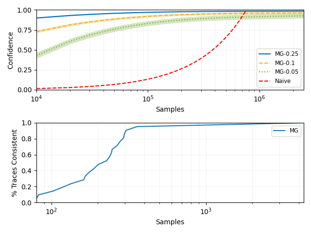
Figure 1: ModelGuard (MG) and Naive approach on mountain car problem, averaged over five trials.

The mean and standard deviation of confidence across the traces labeled inconsistent are presented at the top of Figure 1. Three $\delta$ configurations are presented, showing how the allowed risk of overconfidence affects the confidence. ModelGuard achieves a high confidence, converging on a confidence greater than 0.9. Given the small parameter space, the Naive approach is able to eventually overtake ModelGuard, due to the fact there are a finite number of samples for it to evaluate. The bottom of Figure 1 shows traces were able to be labeled consistent with orders of magnitude fewer samples than what is required to achieve high confidence on inconsistent traces. On average, the number of samples required to label a trace consistent is the same between ModelGuard and the Naive approach, as both involve random samplings of the parameter space.

4.2 Unmanned Underwater Vehicle (UUV)

The second case study is a high-fidelity UUV simulator modified from the work of Manhães et al. (2016), implemented in Gazebo, representing a small, finned craft that is controlled through desired heading and speed setpoints.

The model under consideration is defined as follows. The input space $\mathcal{{U}}=[-\pi,\pi]^{4}\times[0.514,2.5]^{4}$ represents a sequence of desired heading and speed setpoints; parameter space $\mathcal{{X}}=[-0.169,0.17]\times[-0.018,0.018]\times[-0.038,-0.007]\times[-0.053,0.054]$ with no physical meaning; and the output space $\mathcal{{Y}}=[-\pi,\pi]^{5}\times[0.514,2.5]^{5}$ represents a sequence of observed heading and speed for the UUV. The function $G$ is a neural network with a Lipschitz constant of 64.

The tool was evaluated using 36 traces collected from the simulator with half of the traces generated under nominal conditions and the other half collected while the UUV operated with damage to its fin. Using an acceptable error of $\epsilon=0.19$, 21 traces were identified by ModelGuard as consistent with the model. The results of the two approaches are presented in Figure 2.

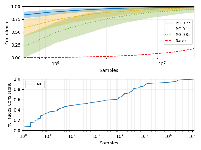
Figure 2: ModelGuard (MG) and Naive approach on UUV problem, averaged over five trials.

Looking at the mean and standard deviation of confidence across the inconsistent traces, presented at the top of Figure 2, we can see that ModelGuard is able to again achieve a high confidence, $>0.8$ on all three $\delta$ configurations. Due to the complexity of the system, the variability between trace confidences is higher. The Naive approach is unable to sufficiently scale to the UUV parameter space, with linear growth making slow progress. We again note, progress on labeling traces consistent is orders of magnitude faster than progress on the confidence of inconsistent traces.

4.3 F1tenth Model Racecar

The final system used for evaluation is the F1tenth model racecar presented by Ivanov et al. (2020). The model racecar is a small autonomous vehicle that uses LIDAR measurements to produce steering controls to drive down a hallway. This is a particularly challenging environment as LIDAR measurements are generally noisy.

The model under consideration is defined as follows. The input space $\mathcal{{U}}=\emptyset$ as the model takes no inputs; parameter space $\mathcal{{X}}=[0,1.5]\times[0,9.9]\times[-\pi/2,\pi/2]$ represents two dimensional position and heading; and output set $\mathcal{{Y}}=[-1.0,1.0]^{21}$ represents the normalized distances from 21 LIDAR rays. The function $G$ is a neural network with a Lipschitz constant of 64.

Out of the real-world LiDAR measurements that were collected as part of the case study by Ivanov et al. (2020), 88 traces was used for evaluation. Using an acceptable error of $\epsilon=0.1948$, 55 traces were identified by ModelGuard as consistent with the model. The results of the two approaches are presented in Figure 3.

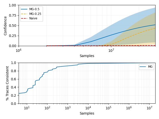
Figure 3: ModelGuard (MG) and the Naive approach on the F1tenth racecar.

The mean and standard deviation of confidence across the traces labeled inconsistent are presented at the top of Figure 3. For this case study, two $\delta$ configurations are presented. On average, ModelGuard achieves a confidence of $~{}0.6$. A high confidence, over 0.9, was reached on many of the traces, however slow progress on the remaining traces drew down the average and resulted in a large standard deviation. The linear growth of the Naive approach is of little use on the large parameter space of the F1tenth model. Again, progress on labeling traces consistent is many orders of magnitude faster than the confidence progress of the inconsistent traces.

4.4 Towards Closing the Loop with ModelGuard

While it can be useful to perform offline analysis on model consistency, we ideally would like to be able to analyze traces in an online manner, identifying situations inconsistent with the model as they happen. To that end, decisions regarding the consistency of a trace should be made quickly. The timing statistics of sample evaluation for each of the case studies are presented in Table 1.

Table 1: Sample Evaluation Time

	Min (us)	Mean (us)	Max (us)
Mountain Car	0.89	2.16	4.00
UUV	3.78	4.82	6.27
F1tenth	8.25	10.60	11.64

While, for these case studies, the amount of time required to label a trace inconsistent with high confidence, and low risk of overconfidence, is infeasible for runtime analysis, the time required to label a trace consistent is less than half of a second. One could imagine a system which considers a trace which has not been labeled consistent after a short period of time to be likely inconsistent and take corrective measures while confidence in the decision increases.

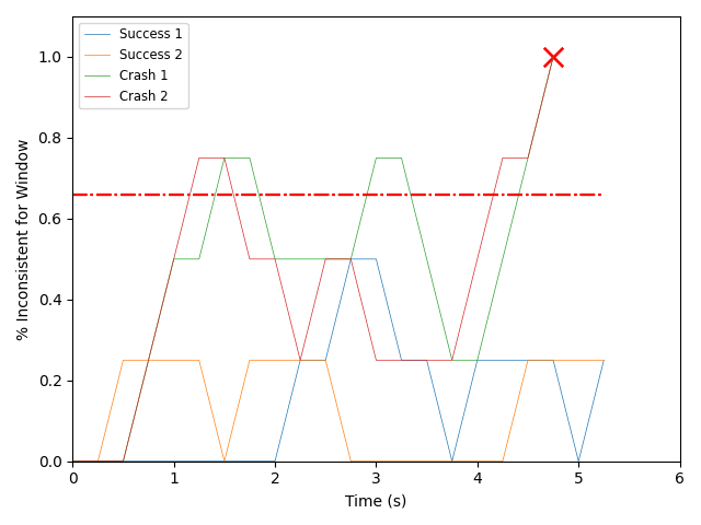
Figure 4: Inconsistency checks over 1 second windows on outputs from four F1tenth trials. Two trials successfully turn and two crash into the wall, marked by the X. The dashed line is a hypothetical monitor threshold.

We present one such scenario in Figure 4, in which two trials of the F1tenth car crash, while two others do not. Consider a safety system for the F1tenth car which monitors consistency of traces over a 1 second sliding window. The monitor alarms if over 2/3 of the window is reported as inconsistent. Such a system would have been able to report an issue 3 seconds before the car crashes.

5 Conclusion and Future Work

This paper presented ModelGuard, a sampling-based approach to validate Lipschitz-continuous models with bounded confidence. In addition to a theoretical backing of the approach, we provided an anytime tool implementation. We also evaluated the applicability and scalability of ModelGuard using three case studies of varying complexity. For future work, we intend to explore sample re-use by investigating how progress on parameter coverage could be carried over between trace evaluations.

Appendix A Proof of Theorem 2

First consider constraint (a). Notice that $h(\bm{u},\bm{y},\mathcal{{X}})\leq h(\bm{u},\bm{y},\mathcal{{X}}_{K})$ as $\mathcal{{X}}_{K}\subset\mathcal{{X}}$. Therefore $h(\bm{u},\bm{y},\mathcal{{X}}_{K})\leq\epsilon\implies h(\bm{u},\bm{y},\mathcal{{X}})\leq\epsilon$; and constraint (a) is satisfied with probability 1.

Next consider constraint (b). Since we are in the case of $\neg\hat{\phi}$, we know that $\forall\bm{x}_{k}\in\mathcal{{X}}_{K}\;\|G(\bm{x}_{k},\bm{u})-\bm{y}\|_{\infty}>\epsilon$. Let $\mathcal{{X}}^{\prime}=C_{\bm{x}_{1}}\cup\dots\cup C_{\bm{x}_{K}}$, then $h(\bm{u},\bm{y},\mathcal{{X}}^{\prime})>\epsilon$, by definition of $C_{\bm{x}_{k}}$. Without loss of generality, we assume $\int_{x\in\mathcal{{X}}}dx=1$ and the remainder of this appendix proves $\bar{\gamma}$ lower bounds $\lambda({\mathcal{{X}}^{\prime}})$ with probability of error that is no greater than $\delta$ – i.e., $\mathbb{P}_{\mathcal{{X}}_{K}}\left[\lambda(\mathcal{{X}}^{\prime})\leq\bar{\gamma}\right]\leq\delta$.

We begin by providing an upper bound on the probability that $\bar{\gamma}$ is not a lower bound, namely

$$\;\mathbb{P}_{\mathcal{{X}}_{K}}\left[\lambda(\mathcal{{X}}^{\prime})\leq\bar{\gamma}\right]$$

$$= \;\mathbb{P}_{\mathcal{{X}}_{K}}\left[\lambda(C_{\bm{x}_{1}}\cup\dots\cup C_{\bm{x}_{K}})\leq\bar{\gamma}\right]$$

$$\leq \;\mathbb{P}_{\mathcal{{X}}_{K}}\left[\lambda(R_{\bm{x}_{1}}\cup\dots\cup R_{\bm{x}_{K}})\leq\bar{\gamma}\right]\ \ \mbox{(since $R_{x}\subseteq C_{x}$)}$$

$$= \;\mathbb{P}_{\mathcal{{X}}_{K}}\left[\int_{x\in\mathcal{{X}}}\mathbbm{1}_{x}(R_{\bm{x}_{1}}\cup\dots\cup R_{\bm{x}_{K}})dx\leq\bar{\gamma}\right]$$

$$= \;\mathbb{P}_{\mathcal{{X}}_{K}}\left[\int_{x\in\mathcal{{X}}}\left(1-\prod_{k=1}^{K}\left(1-\mathbbm{1}_{x}(R_{\bm{x}_{k}})\right)\right)dx\leq\bar{\gamma}\right]$$

$$= \;\mathbb{P}_{\mathcal{{X}}_{K}}\left[\int_{x\in\mathcal{{X}}}\prod_{k=1}^{K}\left(1-\mathbbm{1}_{x}(R_{\bm{x}_{k}})\right)dx\geq 1-\bar{\gamma}\right]$$

$$\leq \;\frac{1}{1-\bar{\gamma}}E_{\mathcal{{X}}_{K}}\left[\int_{x\in\mathcal{{X}}}\prod_{k=1}^{K}\left(1-\mathbbm{1}_{x}(R_{\bm{x}_{k}})\right)dx\right]$$

(above holds due to Markov’s Inequality)

$$= \;\frac{1}{1-\bar{\gamma}}\int_{x\in\mathcal{{X}}}E_{\mathcal{{X}}_{K}}\left[\prod_{k=1}^{K}\left(1-\mathbbm{1}_{x}(R_{\bm{x}_{k}})\right)\right]dx$$

$$= \;\frac{1}{1-\bar{\gamma}}\int_{x\in\mathcal{{X}}}\left(\int_{x^{\prime}\in\mathcal{{X}}}1-\mathbbm{1}_{x}(R_{x^{\prime}})dx\right)^{K}dx$$

$$\leq \;\frac{1}{1-\bar{\gamma}}\int_{x\in\mathcal{{X}}}\left(1-\hat{R}_{x}\right)^{K}dx\;$$

$$\hphantom{\frac{1}{1-\bar{\gamma}}\int_{x\in\mathcal{{X}}}\left(1-\hat{R}_{x}\right)^{K}dx}\mbox{since}\;\hat{R}_{\bm{x}_{j}}\leq\int_{x\in\mathcal{{X}}}\mathbbm{1}_{x}(R_{\bm{x}_{j}})dx$$

$$= \;\frac{1}{1-\bar{\gamma}}E_{\mathcal{{X}}_{K}}\left[\frac{1}{K}\sum_{k=1}^{K}\left(1-\hat{R}_{\bm{x}_{k}}\right)^{K}\right]$$

$$= \;\frac{1}{1-\bar{\gamma}}\left(\frac{1}{K}\sum_{k=1}^{K}\left(1-\hat{R}_{\bm{x}_{k}}\right)^{K}\right)\frac{1}{1-\bar{\gamma}}$$

$$*\left(E_{\mathcal{{X}}_{K}}\left[\frac{1}{K}\sum_{k=1}^{K}\left(1-\hat{R}_{\bm{x}_{k}}\right)^{K}\right]-\frac{1}{K}\sum_{k=1}^{K}\left(1-\hat{R}_{\bm{x}_{k}}\right)^{K}\right)$$

$$\leq \;\frac{1}{1-\gamma}\left(\frac{1}{K}\sum_{k=1}^{K}\left(1-\hat{R}_{\bm{x}_{k}}\right)^{K}\right)\frac{1}{1-\gamma}$$

$$*\left|E_{\mathcal{{X}}_{K}}\left[\frac{1}{K}\sum_{k=1}^{K}\left(1-\hat{R}_{\bm{x}_{k}}\right)^{K}\right]-\frac{1}{K}\sum_{k=1}^{K}\left(1-\hat{R}_{\bm{x}_{k}}\right)^{K}\right|$$

Next, we observe that from Hoeffding’s inequality, for any $c>0$,

$$\;\mathbbm{P}_{\mathcal{{X}}_{K}}\Bigg{[}\frac{1}{K}\sum_{k=1}^{K}\left(1-\hat{R}_{\bm{x}_{k}}\right)^{K}$$

$$\hphantom{\mathbbm{P}_{\mathcal{{X}}_{K}}\Bigg{[}}-E_{\mathcal{{X}}_{K}}\left[\frac{1}{K}\sum_{k=1}^{K}\left(1-\hat{R}_{\bm{x}_{k}}\right)^{K}\right]\Big{|}\geq c\Bigg{]}$$

$$\leq\;2exp\left\{-2Kc^{2}\right\}$$

Combining the two relations above using the law of total probability, we can write

$$\;\mathbb{P}_{\mathcal{{X}}_{K}}\left[\lambda(\mathcal{{X}}^{\prime})\leq\bar{\gamma}\right]$$

$$\leq \;\frac{1}{1-\bar{\gamma}}\left(\frac{1}{K}\sum_{k=1}^{K}\left(1-\hat{R}_{\bm{x}_{k}}\right)^{K}+c\right)$$

$$+2\left(1-\frac{1}{1-\bar{\gamma}}\left(\frac{1}{K}\sum_{k=1}^{K}\left(1-\hat{R}_{\bm{x}_{k}}\right)^{K}+c\right)\right)$$

$$*exp\left\{-2Kc^{2}\right\}$$

$$= \;\frac{1-2exp\left\{-2Kc^{2}\right\}}{1-\bar{\gamma}}\left(\frac{1}{K}\sum_{k=1}^{K}\left(1-\hat{R}_{\bm{x}_{k}}\right)^{K}+c\right)$$

$$\quad+2exp\left\{-2Kc^{2}\right\}$$

We now constrain this upper bound by $\delta$, and observe a constraint on $\bar{\gamma}$, as

$$\;\frac{1-2exp\left\{-2Kc^{2}\right\}}{1-\bar{\gamma}}\left(\frac{1}{K}\sum_{k=1}^{K}\left(1-\hat{R}_{\bm{x}_{k}}\right)^{K}+c\right)$$

$$\;\quad\quad+2exp\left\{-2Kc^{2}\right\}\leq\delta$$

$$\iff \bar{\gamma}\leq 1-a\left(\frac{1}{K}\sum_{k=1}^{K}\left(1-\hat{R}_{\bm{x}_{k}}\right)^{K}+c\right)\;$$

where $a=\frac{1-2exp\left\{-2Kc^{2}\right\}}{\delta-2exp\left\{-2Kc^{2}\right\}}$ and $c=\sqrt{\frac{\ln(2)-\ln(\delta)}{2K}}$. We conclude the proof by observing that $\bar{\gamma}$ satisfies this condition since

$$\frac{\lfloor D\hat{R}_{\bm{x}_{k}}\rfloor}{D}\leq\hat{R}_{\bm{x}_{k}}$$

∎

References

- Borchers et al. (2009) Borchers, S., Rumschinski, P., Bosio, S., Weismantel, R., and Findeisen, R. (2009). A set-based framework for coherent model invalidation and parameter estimation of discrete time nonlinear systems. In Proceedings of the 48th IEEE Conference on Decision and Control.
- Chen et al. (2013) Chen, X., Ábrahám, E., and Sankaranarayanan, S. (2013). Flow*: An analyzer for non-linear hybrid systems. In International Conference on Computer Aided Verification.
- Fazlyab et al. (2019) Fazlyab, M., Robey, A., Hassani, H., Morari, M., and Pappas, G.J. (2019). Efficient and accurate estimation of lipschitz constants for deep neural networks. In Advances in Neural Information Processing Systems.
- Fremont et al. (2019) Fremont, D.J., Dreossi, T., Ghosh, S., Yue, X., Sangiovanni-Vincentelli, A.L., and Seshia, S.A. (2019). Scenic: A language for scenario specification and scene generation. In Proceedings of the 40th annual ACM SIGPLAN conference on Programming Language Design and Implementation.
- Gouk et al. (2020) Gouk, H., Frank, E., Pfahringer, B., and Cree, M.J. (2020). Regularisation of neural networks by enforcing Lipschitz continuity. Machine Learning.
- Ivanov et al. (2019) Ivanov, R., Weimer, J., Alur, R., Pappas, G.J., and Lee, I. (2019). Verisig: verifying safety properties of hybrid systems with neural network controllers. In Proceedings of the 22nd ACM International Conference on Hybrid Systems.
- Ivanov et al. (2020) Ivanov, R., Carpenter, T.J., Weimer, J., Alur, R., Pappas, G.J., and Lee, I. (2020). Case study: Verifying the safety of an autonomous racing car with a neural network controller. In Proceedings of the 23rd International Conference on Hybrid Systems.
- Jin et al. (2020) Jin, Z., Khajenejad, M., and Yong, S.Z. (2020). Data-Driven Model Invalidation for Unknown Lipschitz Continuous Systems via Abstraction. In 2020 American Control Conference. IEEE.
- Manhães et al. (2016) Manhães, M.M.M., Scherer, S.A., Voss, M., Douat, L.R., and Rauschenbach, T. (2016). UUV simulator: A gazebo-based package for underwater intervention and multi-robot simulation. In OCEANS 2016 MTS/IEEE Monterey. IEEE.
- Miyazato et al. (1999) Miyazato, T., Zhou, T., and Hara, S. (1999). A probabilistic approach to model set validation. In Proceedings of the 38th IEEE Conference on Decision and Control.
- Moore (1990) Moore, A.W. (1990). Efficient memory-based learning for robot control. Technical report.
- NHTSA (2017) NHTSA (2017). Investigation pe 16-007. Https://static. nhtsa.gov/odi/inv/2016/INCLA-PE16007-7876.pdf.
- NTSB (2018) NTSB (2018). Preliminary Report Highway HWY18MH010. Https://www.ntsb.gov/investigations /AccidentReports/Reports/HWY18MH010-prelim.pdf.
- Ozay et al. (2014) Ozay, N., Sznaier, M., and Lagoa, C. (2014). Convex Certificates for Model (In)validation of Switched Affine Systems With Unknown Switches. IEEE Transactions on Automatic Control, 59(11).
- Prajna (2006) Prajna, S. (2006). Barrier certificates for nonlinear model validation. Automatica.
- Smith et al. (2000) Smith, R., Dullerud, G., and Miller, S. (2000). Model validation for nonlinear feedback systems. In Proceedings of the 39th IEEE Conference on Decision and Control.
- Szegedy et al. (2013) Szegedy, C., Zaremba, W., Sutskever, I., Bruna, J., Erhan, D., et al. (2013). Intriguing properties of neural networks. arXiv preprint arXiv:1312.6199.