Memory Bounds for Concurrent Bounded Queues

Abstract.

Concurrent data structures often require additional memory for handling synchronization issues in addition to memory for storing elements. Depending on the amount of this additional memory, implementations can be more or less memory-friendly. A memory-optimal implementation enjoys the minimal possible memory overhead, which, in practice, reduces cache misses and unnecessary memory reclamation.

In this paper, we discuss the memory-optimality of non-blocking bounded queues. Essentially, we investigate the possibility of constructing an implementation that utilizes a pre-allocated array to store elements and constant memory overhead, e.g., two positioning counters for enqueue(..) and dequeue() operations. Such an implementation can be readily constructed when the ABA problem is precluded, e.g., assuming that the hardware supports LL/SC instructions or all inserted elements are distinct. However, in the general case, we show that a memory-optimal non-blocking bounded queue incurs linear overhead in the number of concurrent processes. These results not only provide helpful intuition for concurrent algorithm developers but also open a new research avenue on the memory-optimality phenomenon in concurrent data structures.

1. Introduction

Developing concurrent algorithms is complex, and limiting synchronization is crucial in achieving high performance. Mutual exclusions allow building concurrent implementations on top of standard sequential algorithms at the expense of scalability. Non-blocking synchronization has the potential to improve scalability, but it often requires allocating extra memory. The classic Michael-Scott queue (Michael and Scott, 1996) serves as an illustrative example, allocating a new node for each enqueue and, therefore, using a significant amount of memory for node objects; this design results in increased memory usage and cache misses. Modern queues (Gidenstam et al., 2010; Morrison and Afek, 2013; Yang and Mellor-Crummey, 2016) incorporate several elements into a single node, significantly reducing memory allocation and creating a more compact memory structure that mitigates cache misses. We consider these solutions more memory-friendly, as they allocate less additional memory. The intuition is that the more memory-friendly the implementation is, the better and more predictable performance it usually provides under both high and low contention. This is especially important for general-purpose solutions in standard libraries of programming languages and popular frameworks.

In this paper, we raise the question of memory-optimality: what is the absolute minimum of memory overhead a concurrent data structure must incur? We narrow our attention to bounded queues, ubiquitous in resource management systems and task schedulers, e.g., io_uring in Linux kernel (iou, [n. d.]), or high-speed networking and storage libraries such as DPDK (Developers, 2022a) and SPDK (Developers, 2022b). Bounded queues allow for a straightforward definition of memory overhead: the amount of memory that must be allocated on top of the fixed memory required for storing the queue elements.

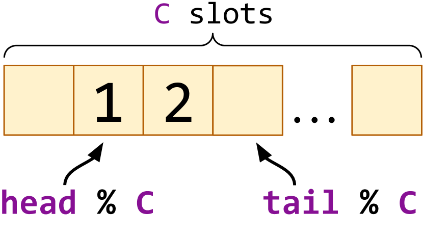
Figure 1. Sequential bounded queue on top of an array of $C$ slots and two counters.

A straightforward sequential bounded queue implementation maintains an array of size $C$ (the queue capacity) equipped with two counters that track the total numbers of enqueue(..) and dequeue() invocations; their values modulo $C$ point to the next working slots of the operations. See Figure 1 for an illustration. This implementation utilizes exactly $C$ array slots to store elements and two memory locations for the counters, producing the $\Theta(1)$ memory overhead.

Can we build a concurrent bounded queue with the same memory footprint? A trivial solution that utilizes coarse-grained locking incurs constant overhead required for the lock but is inefficient under high load. To the best of our knowledge, most fast and scalable concurrent queues are non-blocking, e.g., (Morrison and Afek, 2013; Yang and Mellor-Crummey, 2016; Romanov and Koval, 2023; Nikolaev, 2019). While the classic Michel-Scott queue (Michael and Scott, 1996) algorithm allocates a new node for each element, these modern solutions pack multiple elements into a single node, making the implementation more memory-friendly. Nevertheless, the memory overhead remains linear in the number of elements.

For bounded queues, it is natural to utilize a pre-allocated array of $C$ slots to store elements. This raises an interesting question: is it possible to design an algorithm where the memory overhead depends on neither the queue capacity nor the number of concurrent processes? Can we architect a non-blocking bounded queue using just an array for elements and two positioning counters for enqueue(..) and dequeue(), similarly to the sequential implementation?

Our contribution.

We first observe that the primary challenge in building a concurrent bounded queue is the ABA problem (Herlihy et al., 2020). When the ABA problem is precluded, e.g., when all elements are distinct or using the LL/SC synchronization primitives instead of CAS, we show the possibility of designing an algorithm with constant memory overhead (Section 2).

In the general case, we prove that any obstruction-free (Herlihy et al., 2003) bounded queue implementation must use additional $\Omega(T)$ memory locations for synchronization, where $T$ is the number of processes (Section 3). To show that, we construct a non-linearizable execution for any algorithm that utilizes fewer memory locations. The lower bound appears to be tight: we present an algorithm with $O(T)$ memory overhead.

Practical impact.

In our industrial experience, we witnessed numerous attempts to design a concurrent bounded queue with constant overhead (e.g., on a pre-allocated array with positioning counters). All of these attempts resorted to practical trade-offs like periodic memory allocation, blocking behavior, or relaxed semantics. Our results inform the practitioners that these trade-offs are unavoidable, potentially saving a tremendous amount of time and mental energy for those thinking otherwise.

Notably, most modern unbounded concurrent queues pack multiple elements into fixed-capacity segments and try to reuse them (Romanov and Koval, 2023; Morrison and Afek, 2013; Nikolaev, 2019). These segments, also known as ring buffers, essentially are bounded queues with slightly relaxed semantics, allowing enqueue(..) to fail spuriously and close the segment for further additions. To reuse the segments, they equip each slot with a 64-bit epoch value, leading to $\Theta(C)$ memory overhead, where $C$ is the segment capacity.

Notice that our bounds do not necessarily imply that ring buffers, widely used in real systems, are impractical. However, these ring buffers should relax the semantics, relax the progress guarantee, or employ non-constant memory overhead. While one may share this overhead between multiple bounded queues, our primary result is the impossibility of achieving constant overhead, which significantly affects the algorithm design and its trade-offs.

Theoretical impact.

This work opens a wide research avenue on memory-friendly and memory-optimal concurrent computing. It sets strict bounds on memory overhead in dynamic data structures and provides insights on the optimal memory overhead their implementations can achieve. We believe that the proposed theoretical framework can be extended to other bounded and unbounded data structures, leading to more practical implications.

2. Memory Overhead: The Intuition

We start by developing intuition on memory-friendliness and the challenges in attaining constant memory overhead. To illustrate the latter, we present solutions that work under specific assumptions, thereby shedding light on the fundamental obstacles.

2.1. Simplest Memory-Friendly Queue

We start with a memory-friendly bounded queue algorithm based on the standard linked-list queue. While it is not memory-optimal, it can be tuned to be more or less memory-friendly, thus developing an intuition of memory-friendliness. Note that further we consider implementations that use a more suitable container — the circular buffer.

The idea is to build a bounded queue on a conceptually infinite array with head and tail counters directly pointing to the array slots. Similar to the Michael-Scott queue design (Michael and Scott, 1996), enqueue(..) first installs the element in the next empty slot, followed by the tail counter increment. Similarly, dequeue() begins by extracting the first element, incrementing its tail counter after that. Listing 1 presents the algorithm. As each enqueue-dequeue pair manipulates a unique array slot, the same element cannot be installed into the same slot, so the ABA problem is naturally eliminated.

Infinite array.

We suggest implementing the infinite array as a concurrent linked list of fixed-size segments, following the approach proposed for synchronous queues and channels in Kotlin Coroutines (Koval et al., 2019, 2023). All segments are marked with a unique id and follow each other; Figure 2 illustrates the high-level structure. To access the i-th cell in the infinite array, we find the segment with id = i / K (adding it to the linked list if needed) and go to the cell i % K in it.

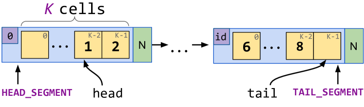
Figure 2. High-level structure of the memory-friendly bounded queue based on a conceptually infinite array implemented via a concurrent linked list of fixed-size segments.

⬇

1fun enqueue(e: E): Bool = while(true) {

2 // Read the counters snapshot

3 t := tail; h := head

4 if t != tail: continue

5 // Is the queue full?

6 if t == h + C: return false

7 // Try to insert the element

8 done := CAS(&a[t], $\perp$, e)

9 // Increment the counter

10 CAS(&tail, t, t + 1)

11 // Finish on success

12 if done: return true

13}

14fun dequeue(): E? = while(true) {

15

16 // Read the counters snapshot

17 t := tail; h := head

18 if t != tail: continue

19 // Is the queue empty?

20 if h == t: return $\perp$

21 // Try to extract an element

22 e := a[h]

23 done := e != $\perp$ && CAS(&a[h], e, $\perp$)

24 // Increment the counter

25 CAS(&head, h, h + 1)

26 // Finish on success

27 if done: return e

28}

Listing 1. Memory-friendly bounded queue of capacity C implemented on an infinite array.

Memory overhead.

Each segment has a memory overhead of $\Theta(1)$ to store its id and a pointer to the next segment. However, we still have to address the memory reclamation problem: once a segment no longer contains queue elements, it should be recycled, and the memory it occupies should be released. To make the memory overhead bounded, we suggest reusing segments by applying the technique to reclaim descriptors (Arbel-Raviv and Brown, 2017). This approach requires $\Theta(T)$ additional segments on top of the ones that store values, where $T$ is the number of concurrent processes. With storing $K$ elements in each segment, the overall solution exhibits $\Theta(C/K\>+\>T\cdot K)$ memory overhead. Though not memory-optimal, this simple algorithm can be tuned to be more or less memory-friendly by adjusting the segment size $K$, achieving the minimum of $\Theta(T\cdot\sqrt{C})$ when choosing $K=\sqrt{C}$.

2.2. Constant Overhead with Distinct Elements

We now describe an algorithm that uses only $O(1)$ additional memory under two reasonable assumptions. First, we require all inserting elements to be distinct, which is common in practice. Second, the system should be provided with an unlimited supply of versioned $\perp$ (null) values, so we can replace unique elements with unique $\perp$-s on extractions. This can be achieved by stealing one bit from addresses (values) to mark them as $\perp$-s and using the rest to store the $\perp$ version. These assumptions help eliminate the ABA problem.

Essentially, both enqueue(..) and dequeue() (1) read the counters in a snapshot manner, (2) try to perform a “round-valid” update (enqueue(..) replaces $\bot_{\mathtt{round}}$ with the element while dequeue() does the opposite, where round = counter / C), and (3) increase the counter via CAS. The pseudocode is presented in Listing LABEL:lst:ppopp.

⬇

1fun enqueue(e: E): Bool = while(true) {

2 // Read the counters snapshot

3 t := tail; h := head

4 if t != tail: continue

5 // Is the queue full?

6 if t == h + C: return false

7 // Try to insert the element

8 round := t / C; i := t % C

9 done := CAS(&a[i], $\perp_{\mathtt{round}}$, e)

10 // Increment the counter

11 CAS(&tail, t, t + 1)

12 // Finish on success

13 if done: return true

14}

15

16fun dequeue(): E? = while(true) {

17 // Read the counters+element snapshot

18 t := tail; h := head; e := a[h % C]

19 if t != tail: continue

20 // Is the queue empty?

21 if t == h: return $\perp$

22 // Try to extract the element

23 round := h / C + 1; i := h % C

24 done := e != $\perp_{\mathtt{round}}$ && CAS(&a[i], e, $\perp_{\mathtt{round}}$)

25 // Increment the counter

26 CAS(&head, h, h + 1)

27 // Finish on success

28 if done: return e

29}

Listing 2: Bounded queue algorithm with $O(1)$ additional memory that requires elements to be distinct and an unlimited supply of versioned $\perp$ (null) values.

2.3. Constant Overhead with LL/SC

Another way to avoid the ABA problem is to use the LL/SC (load-link/store-conditional) ABA-immune synchronization primitives instead of CAS. In this algorithm (Listing LABEL:lst:llsc), both enqueue(..) and dequeue() begin by reading a snapshot of the counters and the corresponding array slot — this part remains unchanged. However, to update the slot state, we now use the SC primitive instead of CAS. By inserting the LL instruction before reading the snapshot, we ensure that the update fails if the cell state has been changed.

The algorithm shows that the LL/SC primitives are conceptually more powerful than CAS. The LL/SC instructions, though not widely available in programming languages, can be used in ARM, PowerPC, RISC-V, and some other architectures (with a certain risk of spurious failures).

2.4. $\Theta(T)$ Overhead with DCSS

Another way to eliminate the ABA problem is to use the Double-Compare-Single-Set (DCSS) synchronization primitive. DCSS(&A, expectedA, updateA, &B, expectedB)

⬇

1fun enqueue(e: E): Bool = while(true) {

2 // Read the counters snapshot

3 t := tail; h := head

4

5 if t != tail: continue

6 // Is the queue full?

7 if t == h + C: return false

8 // Try to insert the element

9

10 // Increment the counter

11 if LL(&tail) == t: SC(&tail, t + 1)

12 // Finish on success

13 if done: return true

14}

15

16fun dequeue(): E = while(true) {

17 // Read the counters+element snapshot

18 h := tail; h := head

19

20 if t != tail: continue

21 // Is the queue empty?

22 if t == h: return $\perp$

23 // Try to extract the element

24

25 // Increment the counter

26 if LL(&head) == d: SC(&head, h + 1)

27 // Finish on success

28 if done: return e

29}

Listing 3: Bounded queue algorithm with $O(1)$ additional memory via LL/SC. This is a modification of the algorithm in Listing LABEL:lst:ppopp; the changes are highlighted.

checks that the values located by addresses A and B are equal to expectedA and expectedB, respectively, updating A to updateA and returning true if the check succeeds, and returning false otherwise.

We use DCSS to atomically update the slot and check that the corresponding counter has not been changed. If DCSS fails, the algorithm helps to increment the counter and restarts the operation. The rest is the same: getting a counters snapshot (including the slot state for dequeue()), checking that the queue is not full/empty, and trying to update the slot state, incrementing the operation counter at the end. Listing LABEL:lst:dcss presents the pseudocode.

For the implementation of DCSS we can use a descriptors approach presented in (Harris et al., 2002). In short, each DCSS call creates a descriptor, which describes the operation, and installs it in the updating location, thus, preventing updates while reading the second location and allowing other threads to help complete the operation. While the naive implementation requires allocating a descriptor object on each DCSS call, it is possible to recycle these descriptors so that only $2T$ of them are required (Arbel-Raviv and Brown, 2017), thus, incurring $\Theta(T)$ additional memory.

⬇

1fun enqueue(e: E): Bool = while(true) {

2 // Read the counters snapshot

3 t := tail; h := head

4 if t != tail: continue

5 // Is the queue full?

6 if t == h + C: return false

7 // Try to insert the element

8

9 // Increment the counter

10 CAS(&tail, t, t + 1)

11 // Finish on success

12 if done: return true

13}

14

15fun dequeue(): E = while(true) {

16 // Read the counters+element snapshot

17 t := tail; h := head

18 e :=

19 if t != tail: continue

20 // Is the queue empty?

21 if t == h: return $\perp$

22 // Try to extract the element

23

24 // Increment the counter

25 CAS(&head, h, h + 1)

26 // Finish on success

27 if done: return e

28}

Listing 4: Bounded queue algorithm with $O(T)$ overhead via recyclable DCSS descriptors. This is a modification of the algorithm in Listing LABEL:lst:ppopp, the changes are highlighted.

2.5. Values and Metadata

Notably, the algorithms with the ‘‘distinct elements’’ assumption (Subsection 2.2) and DCSS (Subsection 2.4) require an ability to store elements and metadata (distinct $\bot$-s and DCSS descriptors) in the same array slots. In practice, to distinguish metadata from data, we either have to steal a bit from values, which results in a smaller universe of possible values, or use language constructs that allow distinguishing types but might lead to a linear memory overhead, such as storing Objects in Java (which incurs boxing when storing primitive values) or using Variant in Rust (which is essentially a wrapper).

3. Memory Overhead: The Lower Bound

Recall that the memory overhead of a bounded queue refers to the extra memory necessary beyond that used to store the elements. We now prove that the minimal memory overhead of a linearizable non-blocking bounded queue is linear in the number of concurrent threads and show that this lower bound is tight by presenting a matching algorithm.

3.1. The Lower Bound: Proof Overview

We proceed by contradiction. Suppose that there exists an obstruction-free linearizable bounded queue of capacity $C$ that employs $X<\frac{T}{24}-1$ value-locations beyond the $C$ memory locations to store the queue elements; $T$ is the number of concurrent threads. (‘‘$24$’’ here is a constant that simplifies the proof without affecting the desired $\Theta(T)$ lower bound.) We construct a non-linearizable execution with such an implementation, showing that any obstruction-free linearizable bounded queue must incur $\Theta(T)$ memory overhead.

To construct a non-linearizable execution, we first catch $X+3$ threads (recall that $X$ is the memory overhead) in a state when they are about to update different memory locations and pause these threads. For simplicity, we assume that these threads will perform writes to the memory locations and never update them to null ($\bot$); we explain how to support updates via CAS and null values later.

Then, carefully ensuring that the queue is empty, we successfully add $C$ elements $x_{1},x_{2},...,x_{C}$ into the queue --- following dequeue()s would have extracted these elements in the same order. However, we do not extract the elements now. Instead, we choose a thread caught right before updating a memory location, which stores an element $x_{i}$ where $1<i<C$, and is about to put $y$ there. Intuitively, this write will remove $x_{i}$ from the middle of the queue and put $y$ instead. As we have caught $X+3$ threads, and the queue uses $X$ additional value-locations, at least three threads are about to update the location where the queue elements are stored and one of them must point to a middle element. Figure 3 illustrates the resulting state.

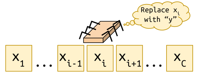
Figure 3. A thread is about to remove $x_{i}$ from the middle of the queue and put $y$ instead.

We now replace the value $x_{i}$ with $y$ by invoking ‘‘write’’ in the caught thread. Assuming the bounded queue implementation does not differentiate elements, the state is now the same as when filling the queue with $x_{1},x_{2},...,x_{i-1},y,x_{i+1},...,x_{C}$ elements. Therefore, the following $C$ dequeue()-s successfully extract these elements.

Intuitively, this execution is non-linearizable, as we have managed to put an element in the middle of the queue, observing ‘‘old’’ elements $x_{1},x_{2},...,x_{i-1}$, then a ‘‘new’’ element $y$, which could not be installed concurrently as the queue is bounded, and followed by ‘‘old’’ elements $x_{i+1},...,x_{C}$.

Note that this is a very simplified version of the proof dedicated to creating an intuition on constructing a non-linearizable execution. To complete the proof, we need to be extremely careful with catching the threads, extending executions, and supporting CAS operations and null values. The following subsections describe the model we use, the reasonable algorithm assumptions that simplify the proof, and the full proof itself.

3.2. Model

Threads and atomic operations.

We consider a system of $T$ processes (threads) $p_{1},\ldots,p_{T}$ communicating by invoking primitives on shared memory. Besides plain reads and writes, we assume Compare-and-Set primitive, denoted as CAS(&a, old, new), that atomically checks the value at address $a$ and, if it equals old, replaces it with new and returns true, returning false otherwise.

While we do not support Fetch-and-Add implicitly, it does not break the proof when not manipulating memory locations where elements are stored. In particular, using Fetch-and-Add for updating counters is allowed.

The LL/SC (load-link/store-conditional) synchronization primitives, however, are not allowed, as they are ABA-immune and enable bounded queue implementation with constant memory overhead, as discussed in Subsection 2.3.

Bounded queue data structure.

The Bounded Queue (BQ) data structure parameterized with type Type and capacity $C$ stores elements of type Type and provides two operations:

• enqueue($x$: Type) (or enq($x$)): if the size of the queue is less than $C$, the operations adds value $x$ and returns true; otherwise, the operation returns false.

• dequeue() (or deq()) retrieves the oldest element from the queue, returning $\perp$ if the queue is empty.

Here, $\perp$ is a special null value, available in most programming languages for references. Also, we omit type Type when discussing BQ.

Implementation.

Informally, an implementation of a bounded queue $BQ$ is a distributed algorithm $A$ consisting of automata $A_{1},\ldots,A_{T}$. Given an operation invoked on $BQ$ by $p_{i}$, $A_{i}$ specifies the sequence of primitive operations on the shared memory that $p_{i}$ needs to execute to compute a response. An execution of an implementation of $BQ$ is a sequence of events: invocations and responses of high-level operations on $BQ$, as well as primitives applied by the processes on the shared-memory locations and the responses they return so that the automata $A_{i}$ and the primitive specifications are respected. An operation is complete in a given execution if a matching response follows its invocation. An incomplete operation can be completed by inserting a matching response after invocation. We only consider well-formed executions: a process never invokes a new high-level operation before its previous operation returns. An operation $o_{1}$ precedes operation $o_{2}$ in execution $\alpha$ (we write $o_{1}\preceq_{\alpha}o_{2}$) if the response of $o_{1}$ precedes the invocation of $o_{2}$ in $\alpha$.

For simplicity, we only consider deterministic implementations: all shared-memory primitives and automata $A_{1},\ldots,A_{T}$ exhibit deterministic behavior. Our lower bound can be, however, easily extended to randomized implementations: in the worst case, we can suggest that a random uses some deterministic algorithm leading to the deterministic execution.

Concurrent execution.

A concurrent execution $\alpha$ of a bounded queue is linearizable  (Herlihy and Wing, 1990; Attiya and Welch, 2004) if all complete operations in it and a subset of incomplete ones can be put in a total order $S$ such that (1) $S$ respects the sequential specification of the bounded queue, and (2) $\preceq_{\alpha}\subseteq\preceq_{S}$, i.e., the total order respects the real-time order on operation in $\alpha$. Informally, every operation $o$ of $\alpha$ can be associated with a linearization point put within the operation’s interval, the fragment of $\alpha$ between the invocation of $o$ and the response of $o$. An implementation is linearizable if any its execution is linearizable.

Progress conditions.

In this paper, we focus on non-blocking implementations that, intuitively, do not involve any form of locking: a failure of a process does not prevent other processes from making progress. We can also talk about non-blocking implementations of specific operations.

Popular liveness criteria are lock-freedom and obstruction-freedom (Herlihy et al., 2020). An implementation of an operation is lock-free if, in every execution, at least one process is guaranteed to complete every such operation it invokes in a finite number of its own steps. An implementation of an operation is obstruction-free if it guarantees that if a process invokes this operation and, from some point on, takes sufficiently many steps in isolation, i.e., without contending with other processes, then the operation eventually competes. We say that an implementation is obstruction-free (resp., lock-free) if all its operations are obstruction-free (resp., lock-free). Lock-freedom is a strictly stronger liveness criterion than obstruction-freedom: any lock-free implementation is also obstruction-free, but not vice versa (Herlihy et al., 2020).

Memory overhead.

Recall that the memory overhead of a bounded queue implementation is the amount of memory that must be allocated on top of the fixed memory required for storing the queue elements.

3.3. Algorithm Restrictions

Atomic operations.

Recall the model supports read, write, and Compare-and-Set operations. For simplicity, we do not support Fetch-and-Add, but it does not break our proof when not manipulating memory locations where elements are stored. In particular, using Fetch-and-Add for updating counters is allowed.

Values and metadata.

We restrict our attention to algorithms that assume a clear separation between value-locations, used exclusively to store queue elements, and metadata-locations, used to store everything else (e.g., counters or descriptors). Importantly, we impose no restrictions on the number of bits that can be stored in memory locations for both metadata and data, allowing metadata-locations to hold either value or metadata. Notably, we require that values and metadata be indistinguishable --- metadata without context can be seen as a value. Making values and metadata distinguishable would require stealing a bit, automatically imposing $\Theta(C)$ memory overhead. Therefore, we find this restriction reasonable. Note that we allow to store $\perp$ (null) in both value- and metadata-locations.

Value-independence.

Furthermore, we assume that the algorithm is agnostic to values: intuitively, the values passed to the operation only reflect the value-locations in the memory and not the steps performed by the algorithm. We call such algorithms value-independent. A value-independent algorithm must be non-creative, enqueue-value-independent and dequeue-value-independent. Intuitively, (1) the implementation of an operation can only manipulate with values stored in value-locations or provided as an argument (if it is an enqueue), (2) it does not matter what is enqueued, $x$ or $y$---the only difference is that $y$’s should be stored instead of $x$’s in the memory, and (3) if the only difference in the memory is $x$ and $y$ in one value-location, a dequeue operation must return $y$ instead of $x$. We present the formal definitions below. To the best of our knowledge, all the state-of-the-art queue implementations satisfy these assumptions.

Definition 3.1.

A BQ algorithm $A$ is non-creative if any value written into a value-location (by write or CAS) during an operation $op$ or returned by it was previously read by $op$ from a value-location or received as an argument (if $op$ is enqueue).

Definition 3.2.

Let $S$ be the memory state reached by an execution $E$ of a BQ algorithm $A$. Suppose $a_{1},\ldots,a_{k}$ and $v$ are distinct values that do not appear in value-locations in $S$. Let a process $p$ be idle in $E$, i.e., it did not execute any operation (neither enqueue nor dequeue) in $E$. Let $S_{1}$ be the memory state reached from $S$ when $p$ sequentially executes enq($a_{1}$), …, enq($a_{i}$), …, enq($a_{k}$) and $S_{2}$ be the memory state of $A$ reached from $S$ when $p$ sequentially executes enq($a_{1}$), …, enq($v$),…, enq($a_{k}$) ($v$ is inserted instead of $a_{i}$). $A$ is enqueue-value-independent if $S_{1}$ is identical to $S_{2}$, except that every value-location storing $a_{i}$ in $S_{1}$ stores $v$ in $S_{2}$.

Definition 3.3.

Let $S$ be a memory state reached by some execution $E$ of a BQ algorithm $A$. Suppose that there is a value $x$ that appears only in one value-location in $S$ and let process $p$ be idle in $E$. Let process $p$ sequentially apply dequeue() operations as long as they are successful, i.e., until the queue becomes empty, and suppose that exactly one of these dequeue() operations $op$ returns $x$. $A$ is dequeue-value-independent if replacing $x$ with $y$ in $S$ and replaying dequeue() operations by process $p$, we obtain an execution of $A$ in which $op$ now returns $y$.

Definition 3.4.

A BQ implementation $A$ is value-independent if it is non-creative, enqueue-value-independent, and dequeue-value-independent.

3.4. Auxiliary Notions

Definition 3.5.

In the proof, we construct an execution where some processes are paused just before performing $CAS(l,x,y)$ operation. Such processes are called poised, and the location $l$ is said to be covered by that process.

For simplicity, we treat $\textsf{l.write}(y)$ as $CAS(l,\ast,y)$ with ‘‘$\ast$’’ matching any value.

Definition 3.6.

If a value $v$ was never used as an argument in the execution $E$, we say that $v$ is fresh in $E$.

Let $E$ be a finite execution of $A$, and $p$ be an idle process in $E$. A fill procedure applied to $E$ (or just fill) consists of a process $p$ enqueueing $C$ different values in isolation. We say that a fill procedure is successful if all $C$ enqueues are successful and $C$ different value-locations store these values.

An empty procedure (or just empty) consists of process $p$ executing $C$ dequeue operations in isolation. We say that an empty procedure is successful if all these $C$ dequeue operations are successful.

We say that a fill-empty-procedures pair is up-to-date if both procedures are successful and dequeues from the empty procedure return the values enqueued by the fill.

Lemma 3.7.

Every finite execution has a solo extension (where only a single process takes steps) that ends with an up-to-date fill-empty procedure.

To prove Lemma 3.7, we need the following lemmas first.

Definition 3.8.

We say that the queue is logically empty if it is in a state for which a new dequeue operation would return $\perp$ if executed in isolation.

Lemma 3.9.

Let $S$ be a memory state produced by an execution $E$ in which the queue is logically empty queue and some of the processes are poised. If we extend $E$ with a fill procedure followed by an empty procedure and one of these procedures is not successful, then one of the operations executed by the posed processes “took effect”, i.e., is linearized before any future operation.

Proof.

We have a logically empty queue and we perform a fill procedure. Suppose this fill is not successful. By definition, there can be two cases. First, some enqueue operation is not successful then another enqueue operation succeded (exactly, $C$ enqueues succeed) — which can only be the one that was poised and, thus, it is linearized. Second, all enqueue operations are successful, but not all $C$ new values are stored in the shared memory. Thus, there exists some poised dequeue operation that can return the non-stored value. But after the successful empty procedure, it would mean that this poised operation is linearized.

After the fill procedure, the logical state of the queue is full. Thus, $C$ dequeues should succeed. If the empty procedure is not successful, thus, some old poised dequeue takes place. This means that it was already linearized before that moment. ∎

Lemma 3.10.

Consider some state of a system: a logically empty queue with poised operations. If we perform a successful fill procedure followed by a successful empty procedure and dequeue operations of the empty procedure return not the exactly same values that were enqueued by the fill procedure, then one of the poised operations “took effect”.

Proof.

Let us look at the value $v$ that was enqueued and was not dequeued by the empty procedure. In the end, the queue is empty; thus, the value $v$ was dequeued by some operation. Since it was not returned by any operation from the empty procedure, it should be some poised operation. Thus, after the empty procedure, this poised operation is linearized. ∎

By combining the last two lemmas, we construct the following result.

Lemma 3.11.

Consider some state of a system: a logically empty queue with poised operations. If a fill-empty-procedures pair applied to this state is not up-to-date, then one of the poised operations “took effect”, i.e., is linearized before any future operations.

We are now ready to prove Lemma 3.7 and show that every execution can be extended by one working process with an up-to-date fill-empty procedure at the end.

Proof of Lemma 3.7.

In our proof, a dedicated process repeatedly performs alternating fill and empty procedures, until the corresponding pair is up-to-date. By Lemma 3.11, the number of such iterations cannot exceed $T$, as in our proof we catch at most $T-1$ concurrent operations ∎

3.5. The Lower Bound: Complete Proof

We now present a complete proof of the memory overhead lower bound. Specifically, we prove Theorem 3.12 below.

Theorem 3.12.

Any obstruction-free linearizable value-independent implementation of Bounded Queue with capacity $C$ uses $C+\lfloor\frac{T-24}{24}\rfloor$ value-locations, assuming that there exists at least $\Theta(T\cdot C)$ different values and $\frac{T}{2}<C$.

Recall that the key idea is to construct a non-linearizable execution. Before diving deeper into details, we describe the execution we target to construct and prove that it is non-linearizable.

Lemma 3.13.

Let $k=2X+3$. Let $E$ be an execution that results in a state that has $k$ value-locations $l_{1},\ldots,l_{k}$, which store distinct values $x_{1},\ldots,x_{k}$, and $x_{i}$ can be replaced with $y_{i}$ in each value-location $l_{i}$ by poised CAS-s. Also, all $x_{i}$ are distinct, and for all $i$, $x_{i}\neq y_{i}$, and $x_{i},y_{i}$ are non-$\bot$.

Then we can extend $E$ to a non-linearizable execution.

Proof.

First, we extend $E$ using one process so it ends with up-to-date fill-empty pair (by Lemma 3.7, this is possible). By the definition of a successful fill, there are $C$ distinct values stored in value-locations after it, so, since we have $C+X$ value-locations in total, there are at least $C-X$ of these new values that are not duplicated in value-locations, i.e. each of them appears in exactly one value-location. As $k=2X+3$, after the fill, there are at least $3$ locations among $l_{1},\ldots,l_{k}$ such that a value of some enqueue from fill is stored only in that location. Thus, there is $l_{i}$ that stores a value of some $enq$ from the fill procedure that is not a first $enq$, nor the last one, and this value is stored only in $l_{i}$. Using enqueue-value-independence we change the argument of the corresponding enqueue to $x_{i}$, reaching the state where after the fill $l_{i}$ is the only location storing $x_{i}$ and $x_{i}$ is returned in the following empty procedure.

Therefore, if we replay this updated fill procedure we could perform poised CAS-s substituting $x_{i}$ with $y_{i}$ before the empty procedure. Thus, if at this point we replay the empty procedure, the dequeue that used to return $x_{i}$ now returns $y_{i}$ by dequeue-value independence.

By that, the last fill-empty-procedures pair have operations

$enq(v_{1})$	$\cdots$	$enq(x_{i})$	$\cdots$	$enq(v_{C})$
$deq\rightarrow v_{1}$	$\cdots$	$deq\rightarrow y_{i}$	$\cdots$	$deq\rightarrow v_{C}$

We call a pair of type $\langle enqueue(v),\ dequeue\rightarrow v\rangle$ a matching pair and it is true-matching if in any given linearization, these enqueue and dequeue indeed match each other.

We claim that $\langle enq(v_{1}),deq\rightarrow v_{1}\rangle$ and $\langle enq(v_{C}),deq()\rightarrow v_{C}\rangle$ are true-matching pairs in the constructed execution.

To see this, note that for a matching pair to be not true-matching there should be another enqueue whose value is dequeued. But $v_{1}$ and $v_{C}$ are fresh values since the only non-fresh value among enqueues is $x_{i}$ and by the construction, it is not the last, nor the first enqueue. Thus, there can not be other poised $enq(v_{1})$ or $enq(v_{C})$.

The question now is where to place $enq(y_{i})$ to find a true-match ${deq\rightarrow y_{i}}$. It cannot be placed before $enq(v_{1})$ or after $enq(v_{C})$ since the pairs for $v_{1}$ and $v_{C}$ are true-matching and they cannot transpose due to FIFO property of the queue. So, it can only be placed between $enq(v_{1})$ and $enq(v_{C})$.

But then we have $C+1$ successful enqueues in a row, so there must be $deq\rightarrow v_{1}$ before $enq(v_{C})$ which means that the pair $\langle enq(v_{1}),deq\rightarrow v_{1}\rangle$ from the table is not a true-match, but we have proven it already.

Thus, $enq(x_{i})$ corresponds to $deq\rightarrow y_{i}$ which makes the execution not linearizable. ∎

We are finally ready to prove the main Theorem 3.12 and show that any obstruction-free linearizable value-independent implementation of Bounded Queue with capacity $C$ uses $C+\lfloor\frac{T-24}{24}\rfloor$ value-locations, assuming that there exists at least $\Theta(T\cdot C)$ different values and $\frac{T}{2}<C$.

Proof of Theorem 3.12.

The proof proceeds by contradiction. Namely, we pick the number of additional value-locations $X$ small enough, though still linear in $T$, and show that for each implementation that uses at most $X$ additional value-locations, we can build a non-linearizable execution. We prove that it is sufficient to pick $X=\lfloor\frac{T-24}{24}\rfloor$.

Our procedure to create non-linearizable execution is partitioned into four steps. During the first step, the queue is filled with fresh values, and $\frac{T}{2}$ processes are poised right before the CAS operation. In the second step, we just call empty and fill procedures in order to obtain fresh values in memory. The third and fourth steps are the most complicated. Depending on the BQ algorithm, we get three cases depending on poised operations. The goal of each case is to come up with an execution that brings the queue to the state required by Lemma 3.13. Finally, using this lemma we build a non-linearizable execution.

Now, we dive into the details. Our construction algorithm works in four steps.

First step.

We try to extend an execution $\frac{T}{2}$ times with an up-to-date fill-empty pair using Lemma 3.7. For each pair, we require a new idle process, i.e., a process that has not started any operation. Though, for each try, we don’t let a process finish an extension, rather we stop this process right before it is about to CAS at a not yet covered value-location from $\bot$. We say that we catch the process when we stop it right before performing a CAS. When we catch the process, we restart with another process using Lemma 3.7. We claim that using this procedure we can catch $\frac{T}{2}$ processes.

To see that, assume by the contrary that we do not catch $\frac{T}{2}$ processes. Thus, one of them managed to perform a successful fill. By the definition of successful fill, there must be $C$ fresh values stored in the value-locations after it, so a process made successful attempts to CAS $C$ value-locations and was not poised. This implies that all those locations are covered since all locations initially store $\bot$ and hence cannot be modified without being previously covered. But since one process covers only one location and $C>\frac{T}{2}$, $C$ locations cannot be covered, a contradiction.

Second step.

We extend an execution using a new idle process to end up with a successful fill. It is indeed possible by the trivial corollary of the Lemma 3.7: if we can ensure successful fill and empty, we can just stop after the fill.

Third step.

We try to extend an execution $\frac{T}{2}$ times with an up-to-date fill-empty pair using Lemma 3.7. For each pair, we require a new idle process. Though, for each try, we do not let a process finish an extension, rather we stop this process right before it is about to CAS on a location that satisfies the following catch criteria:

1. The corresponding value-location was not yet covered by some CAS at Step 3;

2. This value-location is already covered by some CAS at Step 1;

3. The poised CAS must be from a non-bottom value different from the previous CAS-s poised during Step 3.

Fourth step.

This step is to account for the case when there are few processes caught at Step 3.

If there are $\frac{T}{4}-3X$ idle processes at this point, we consecutively extend the execution with a successful fill using each of them. It is indeed possible by the trivial corollary of the Lemma 3.7. We catch a process if it satisfies the following catch criteria:

1. The corresponding value-location is not yet covered by CAS at Step 4;

2. This value-location is already covered by CAS at Step 1;

3. The poised CAS must be from a non-bottom value (to possibly a bottom one) different from the previous CAS-s poised during Step 4.

Now, we explain how our poised operations provide a state desired by Lemma 3.13. This part becomes a little bit technical — we get three cases depending on how many CAS-s we poised during Step 3:

• Suppose that we poised less than $\frac{T}{4}$ processes.

  After Step 2, the successful fill is performed, so $C$ fresh distinct values are stored in $C$ different locations. We have $\frac{T}{2}$ value-locations covered by CAS-s at Step 1, so, since we have $C+X$ value-locations in total, there are $\frac{T}{2}-2X$ locations among covered that store unique values. Let us call the set of these locations that are not modified during Step 3 as $L^{\prime}$. We claim that $|L^{\prime}|>\frac{T}{4}-2X$.

  To see this, assume the opposite, namely that $L^{\prime}$ has at most $\frac{T}{4}-2X$ value-locations. Then at least $(\frac{T}{2}-2X)-|L^{\prime}|=\frac{T}{4}$ of our chosen value-locations were modified. It means that during our procedure in Step 3, we made a CAS on these locations but did not catch it. This could happen only if one of the catch criteria of Step 3 was not satisfied. However, criteria (2) and (3) are always satisfied due to the way we chose locations: the chosen value-locations are already covered by some CAS from Step 1, and they stored non-bottom value (they store some of $C$ values from Step 2). Thus, the only criterion that could not be satisfied is (1), i.e., it is already covered by a CAS. But, we poised less than $\frac{T}{4}$ CAS-s in the main condition; thus, (1) is satisfied for some location — we could have poised at least one more CAS. Thus, $|L^{\prime}|$ is greater than $\frac{T}{4}-2X$.

  We claim that during Step 4, we catch $\frac{T}{4}-3X$ processes. Otherwise, one of them was able to complete a successful fill, which implies that $C$ fresh values are stored, so at most $X$ locations are left unmodified. Thus, at least $|L^{\prime}|-X=\frac{T}{4}-3X$ locations in $L^{\prime}$ must be overwritten – there will be attempts to successfully CAS and hence cover them. Let $L$ be the set of value-locations covered by poised operations from Step 4. Finally, we apply Lemma 3.13 with $l_{i}$ being locations from $L$.

  We now need to show that the Lemma 3.13 requirements are satisfied. By the construction of $L$, all $l_{i}\in L$ are indeed distinct. For each $1\leq i\leq|L|$ there is a poised CAS of the form $CAS(l_{i},\bot,y_{i})$ and a CAS of the form $CAS(l_{i},x_{i},mb_{i})$. If $mb_{i}\neq\bot$, then we can change the value in $l_{i}$ from $x_{i}$ to $mb_{i}$. Otherwise, we can perform both CAS-s changing the value in $l_{i}$ from $x_{i}$ to $y_{i}$. We also need to show that all $x_{i}$ are distinct. It follows from the fact that all values in $L^{\prime}$ are. Finally, $|L|=\frac{T}{4}-3X\geq 2X+3$, thus, we can choose $2X+3$ locations from $L$ and apply Lemma 3.13.

• Suppose that in Step 3 at least $\frac{T}{4}$ processes are poised while more than $\frac{T}{8}$ of them CAS to non-bottom.

  Let $L$ be the set of value-locations covered by poised CAS-s updating to non-bottom.

  Now, we can apply Lemma 3.13 with $l$-s being locations from $L$.

  Let us check Lemma’s requirements are satisfied. Locations in $L$ are distinct by the catch criteria. We can indeed substitute $x_{i}$ with $y_{i}$ in each $l_{i}$ applying the corresponding CAS. $x_{i}$ are non-bottom because of the catch criteria and $y_{i}$ are non-bottom because of the current case assumption. All $x_{i}$ are distinct because of the catch criteria. Finally, $|L|\geq\frac{T}{8}\geq 2X+3$, thus, we can choose $2X+3$ locations from $L$ and apply Lemma 3.13.

• Suppose that in Step 3 at least $\frac{T}{4}$ processes are poised and at least $\frac{T}{8}$ of them CAS to bottom.

  Here, we have at least $\frac{T}{8}$ pairs of the type $CAS(l_{i},\bot,y_{i})$ and $CAS(l_{i},x_{i},\bot)$.

  Note that $x$-s are those values that were present in the memory after Step 2, whereas $y$-s are those introduced during Step 1. Recall that by non-creative property $y$-s are all arguments of enqueue operations.

  Filling the queue with fresh values in Step 2 guarantees that at most $X$ values out of those $y$-s are present at the start of Step 3. Since all $x$-s are pairwise distinct by the catch criteria of Step 3, there can be no more than $X$ values from $y$-s among them. We no longer consider CAS pairs where CAS is done from $x$ which is equal to some $y_{i}$. However, there are at most $X$ of the non-satisfying pairs and we still have at least $\frac{T}{8}-X$ good $CAS(l_{i},\bot,y_{i}),CAS(l_{i},x_{i},\bot)$ pairs. Let $L=\{l_{i}\}$ be the set of value-locations covered by these pairs.

  Finally, we can apply Lemma 3.13 with $l_{i}$ being elements of $L$.

  Requirements of the Lemma are satisfied. Indeed, $l$-s are distinct and $x$-s are distinct by the catch criteria of Step 3. For each $l_{i}$ we can substitute $x_{i}$ with $y_{i}$ performing a pair of CAS-s. Moreover, $x$-s are distinct from $y$-s, since $y$-s are values from Step 1 and by the construction of $L$ there are no values from Step 1. Finally, $|L|=\frac{T}{8}-X\geq 2X+3$, thus, we can choose $2X+3$ locations from $L$ and apply Lemma 3.13.

∎

System-wide overhead.

Intuitively, one may share the overhead between multiple queues. Specifically, when using $k$ obstruction-free bounded queues of capacity $C$, the total memory overhead might remain $O(T)$ (not depending on $k$). However, our primary result is the impossibility of achieving constant overhead in a single bounded queue, significantly affecting the algorithm design and its trade-offs.

3.6. The Upper Bound

Finally, we show that our lower bound is tight by presenting an algorithm that asymptotically matches the lower bound and uses $O(T)$ extra memory. Please note that our goal is to show the upper bound of the memory overhead rather than provide a practical and efficient implementation.

Algorithm overview.

The key idea is to use descriptors for enqueue(..) operations, with the possibility of reusing them (Arbel-Raviv and Brown, 2017), to match the desired memory overhead. In addition, we use an $T$-size ‘‘announcement’’ array that stores references to descriptors of ‘‘in-progress’’ enqueue(..) invocations. Intuitively, a descriptor in this array declares an intention to perform an enqueue operation on some chosen cell. This enqueue succeeds if the enqueues counter has not been changed (which is similar to our DCSS-based solution above). The descriptor stores a target cell to write and an operation status in successful field. We say that a descriptor/operation/thread ‘‘covers’’ a cell if it intends to put an element there.

Thus, in total, we have $O(T)$ memory overhead that asymptotically matches the lower bound shown in the previous subsection.

Now, we explain how descriptors and the announcement array help us achieve a correct algorithm. As in the previous algorithms, a dequeue() (resp., enqueue(..)) operation starts with taking a snapshot of the counters in lines and checks if the queue is empty (resp., full).

The implementation of dequeue() slightly differs from those in the algorithms from Section 2. To read an element, it goes through the announcement array to check for the ongoing enqueue operations on the target cell, which is calculated from the counters. If one exists, our dequeue takes the argument of that ongoing operation. Otherwise, it takes a value from the target cell. Finally, it tries to increment the dequeues counter and returns the found element if the corresponding CAS succeeds.

As for enqueue(..), it creates a special descriptor, announces it in our announcement array, and then tries to atomically apply the operation. Then, the operation increments the enqueues counter, possibly helping some concurrent operation. If the descriptor is successfully applied, the operation completes. Otherwise, the operation is restarted.

There can be only one descriptor in the successful state that can ‘‘cover’’ a given cell in the elements array, no other successful descriptor can point to the same cell. Thus, only the thread that started covering the cell is eligible to update it. When the thread with exclusive access for modifications finishes the operation, it ‘‘releases’’ the cell, so, another operation is able to ‘‘cover’’ it. However, when an enqueue operation finds a cell to be covered, it replaces the old descriptor (related to the thread that covers the cell now) with a new one and completes. The thread with the exclusive access to the cell helps this enqueue operation to put the element.

Summing everything up, our algorithm is lock-free (Appendix A.1) and it uses just $O(T)$ additional memory to $C$ values in the bounded queue. Please note that we do not provide any guarantees about the execution time of operations on our BQ. One should expect the queue to answer the queries in $O(1)$, however, in our algorithm each operation should traverse through the whole announcement array leading to $\Theta(T)$ time. This leaves us with an open question whether it is possible to implement a memory-optimal queue that serves requests in $O(1)$ time.

Implementation details.

We discuss the implementation details and prove the algorithm’s correctness in Appendix A.

4. Related Work

Memory efficiency has always been one of the central concerns in concurrent computing. Many theoretical bounds have been established on memory requirements of various concurrent abstractions, such as mutual exclusion (Burns and Lynch, 1993), perturbable objects (Jayanti et al., 2000), or consensus (Zhu, 2016). However, it appears that minimizing memory overhead in dynamic concurrent data structures has not been in the highlight until recently. A standard way to implement a lock-free bounded queue, the major running example of this paper, is to use descriptors (Valois, 1994; Pirkelbauer et al., 2016) or additional meta-information per each element (Tsigas and Zhang, 2001; Vyukov, [n. d.]; Shafiei, 2009; Feldman and Dechev, 2015). The overhead of resulting solutions is proportional to the queue size: a descriptor contains an additional $\Omega(1)$ data to distinguish it from a value, while an additional meta-information is $\Omega(1)$ memory appended to the value by the definition.

The fastest queues, however, store multiple elements in nodes so the memory overhead per element is relatively small from the practical point of view (Morrison and Afek, 2013; Yang and Mellor-Crummey, 2016; Romanov and Koval, 2023), and we consider them as memory-friendly, though not memory-optimal.

A notable exception is the work by Tsigas et al. (Tsigas and Zhang, 2001) that tries to answer our question: whether there exists a lock-free concurrent bounded queue with $O(1)$ additional memory. The solution proposed in (Tsigas and Zhang, 2001) is still a subject to the ABA problem even when all the elements are different: it uses only two null-values, and if one process becomes asleep for two ‘‘rounds’’ (i.e., the pointers for enqueue(..) and dequeue() has made two traversals through all the elements), waking up it can incorrectly place the element into the queue. Besides resolving the issue, our algorithm, under the same assumptions, is shorter and easier to understand (see Subsection 2.2).

The tightest algorithm we found is the recent work by Nikolaev (Nikolaev, 2019), that proposes a lock-free bounded queue with capacity $C$ implemented on top of an array with $2C$ memory cells. While the algorithm manipulates the counters via Fetch-And-Add, it still requires descriptors, one per each ongoing operation. This leads to the additional overhead linear in $T$. Thus, the total memory overhead is $\Omega(C+T)$, while the lower bound is $\Theta(T)$ and does not depend on the queue capacity.

5. Discussion

In this paper, we proved that any non-blocking implementation of a bounded queue incurs $\Omega(T)$ memory overhead, while showing that the bound is asymptotically tight with a matching algorithm. In Section 2, we also presented a series of algorithms with constant memory overhead that work under several practical restrictions on the system or/and the application, along with a simple DCSS-based algorithm that matches the lower bound but requires an ability to store values and descriptors in the same array slot.

We find the following relaxations important to consider in future work: (1) the single-producer and single-consumer application restrictions, (2) the ability to store descriptors in value-locations (free in JVM and Go) or ‘‘steal’’ a couple of bits from addresses (free in C++) for containers of references, and (3) relaxing the object semantics, e.g., to probabilistic guarantees. Each of these cases corresponds to a popular class of applications, and determining the optimal memory overhead in these scenarios is appealing in practice.

It would also be interesting to consider the problem of memory overhead incurred by wait-free implementations since such solutions are typically more complicated.

Finally, in this paper, we only focused on bounded queues, as they allow a natural definition of memory overhead. One may try to extend the notion to the case of unbounded queues by considering the ratio between the amount of memory allocated for the metadata with respect to the memory allocated for data elements. Defining the bounds on this ratio for various data structures, such as pools, stacks, etc., remains an intriguing open question.

Appendix A Memory-Optimal Bounded Queue

In this section we present an algorithm (Figure 7) that exhibits $O(T)$ memory overhead only using read, write, and CAS primitives. In Section 3.5, we showed that the algorithm is (asymptotically) memory-optimal.

To address the ABA problem, in our algorithm, enqueue(..) operations use descriptors stored in pre-allocated metadata locations (each descriptor takes $\Theta(1)$ memory). To enable recycling (Arbel-Raviv and Brown, 2017), we allocate $2\cdot T$ descriptors. For simplicity, we omit that from the pseudo-code: but this reclamation procedure indeed happens. In addition, an $T$-size ‘‘announcement’’ array is used to store references to the descriptors. Altogether, this gives $O(T)$ memory overhead.

As in the previous algorithms, a dequeue() (resp., enqueue(..)) operation starts with taking a snapshot of the counters in lines 29--31 (resp., lines 36--37)), and checks if the queue is empty in line 32 (resp., full in line 38).

Overview.

The implementation of dequeue() slightly differs from those in the algorithms from Section 2 above. To read an element to be retrieved during the snapshot (line 30), it uses a special readElem function. Then it tries to increment the dequeues counter and returns the element if the corresponding CAS succeeds (line 33).

As for enqueue(..), it creates a special EnqOp descriptor (declared in lines 1--21) and then tries to atomically apply the operation (line 39). Then the operation increments the enqueues counter, possibly helping a concurrent operation (line 40). If the descriptor is successfully applied, the operation completes. Otherwise, the operation is restarted.

The algorithm maintains an array ops of EnqOp descriptors (line 24), which specifies ‘‘in-progress’’ enqueue(..) invocations. Intuitively, an EnqOp descriptor declares an intention to perform an enqueue operation that succeeds if the enqueues counter has not been changed (which is similar to our DCSS-based solution above). The descriptor stores an operation status in successful field (line 10). We say that a descriptor/operation/thread ‘‘covers’’ a cell if it has an intention to put an element there.

There can be only one descriptor in the successful state that can ‘‘cover’’ a given cell in the elements array a, no other successful descriptor can point to the same cell (see putOp function in lines 45--58). Thus, only the thread that started covering the cell is eligible to update it. When the thread with an exclusive access for modifications finishes the operation, it ‘‘releases’’ the cell (see function completeOp in lines 69--73), so, another operation is able to cover it. However, when an enqueue operation finds a cell to be covered, it replaces the old descriptor (related to the thread that covers the cell now) with a new one and completes (lines 89-92). The thread with the exclusive access to the cell helps this enqueue operation to put the element into a.

⬇

1// Descriptor for enqueues

2class EnqOp<T>(enqueues: Long,

3 element: Type) {

4 val e = enqueues // ‘enqueues‘ value

5 val x = element // the inserting element

6 val i = e % C // cell index in ‘a‘

7 // Op status: true, false, or $\perp$;

8 // we consider $\perp$ as the second

9 // ’false’ in logical expressions.

10 var successful: Bool? = $\perp$

11

12 fun tryPut(): // performs the logical put

13 // Is there an operation which

14 // already covers cell ’i’?

15 (op, opSlot) := findOp(i)

16 if op != $\perp$ && op != this:

17    CAS(&successful, $\perp$, false)

18 // Has ’enqueues’ been changed?

19 eValid := e == enqueues

20 CAS(&successful, $\perp$, eValid)

21}

22

23// Currently running enqueues

24var ops: EnqOp?[] = new EnqOp?[T]

25// The next operation to be applied

26var activeOp: EnqOp? = $\perp$

27

28func deq() Type? = while (true):

29    d := dequeues; e := enqueues

30    x := readElem(d % C)

31    if d != dequeues: continue

32    if e == d: return $\perp$

33    if CAS(&dequeues, d, d + 1): return x

34

35func enq(x: Type) Bool = while (true):

36    e := enqueues; d := dequeues

37    if e != enqueues: continue

38    if e == d + C: return false

39    op := new EnqOp(e, x); apply(op)

40    CAS(&enqueues, e, e + 1)

41    if op.successful: return

42

43// Puts ’op’ into ’ops’ and returns

44// its location, or -1 on failure.

45func putOp(op: EnqOp) Int:

46 for j in 1..$\infty$:

47    opSlot := j % T

48

49    if !CAS(&ops[opSlot], $\perp$, op):

50       continue // occupied

51    startPutOp(op)

52    op.tryPut() // logical addition

53    // Finished, free ‘activeOp‘.

54    CAS(&activeOp, op, $\perp$)

55    if !op.successful:

56       ops[opSlot] = $\perp$ // clean the slot

57       return -1

58    return opSlot

Listing 6: Bounded queue algorithm with $O(T)$ overhead via recyclable DCSS descriptors. This is a modification of the algorithm in Listing LABEL:lst:ppopp, the changes are highlighted.

⬇

59// Starts the ’op’ addition.

60func startPutOp(op: EnqOp) = while (true):

61    cur := activeOp

62    if cur != $\perp$: // need to help

63       cur.tryPut()

64       CAS(&activeOp, cur, $\perp$)

65    if CAS(&activeOp, $\perp$, op): return

66

67// Only the thread that covers the

68// cell is eligible to invoke this.

69func completeOp(opSlot: Int) = while (true):

70    op := readOp(opSlot) // not $\perp$

71    a[op.i] = op.x

72    CAS(&enqueues, op.e, op.e + 1)

73    if CAS(&ops[opSlot], op, $\perp$): return

74

75// Tries to apply ’op’.

76func apply(op: EnqOp):

77 (cur, opSlot) := findOp(op.i)

78 // Try to cover the cell by ’op’.

79 if cur == $\perp$:

80    opSlot = putOp(op)

81    // Complete ‘op‘ if the cell is covered

82    if opSlot != -1: completeOp(opSlot)

83    return

84 // ’cur’ already covers the cell.

85 if cur.e >= e: // is ’op’ outdated?

86    op.successful = false

87    return

88 // Try to replace ’cur’ with ’op’.

89 op.successful = true

90 if CAS(&ops[opSlot], cur, op): return

91 // The replacement failed.

92 op.successful = false

93

94// Looks for ’EnqOp’ that covers cell

95// ’i’, returns ’a[i]’ if not found.

96func readElem(i: Int) Type:

97 (op, _) := findOp(i)

98 if op != $\perp$: return op.elem

99 return a[i] // EnqOp is not found

100

101// Returns the operation located at

102// ’ops[opSlot]’ if it is successful.

103func readOp(opSlot: Int) EnqOp?:

104 op := ops[opSlot]

105 if op != $\perp$ && op.successful: return op

106 return $\perp$

107

108// Returns a successful operation that

109// covers cell ’i’, $\perp$ otherwise.

110func findOp(i: Int) (EnqOp?, Int):

111 for opSlot in 0..n-1 {

112    op := readOp(opSlot)

113    if op != $\perp$ && op.i == i:

114       return (op.value, opSlot)

115 return $\perp$ // not found

Listing 7: Bounded queue algorithm with $O(T)$ overhead via recyclable DCSS descriptors. This is a modification of the algorithm in Listing LABEL:lst:ppopp, the changes are highlighted.

Listing 7. Bounded queue algorithm with $\Theta(T)$ overhead.

Reading an element.

Once a dequeue() operation reads the first element (line 30), it cannot simply read cell a[d % C], as there can be a successful EnqOp in ops array which covers the cell but has not written the element to the cell yet. Thus, we use a special readElem function (lines 96--99), which goes through array ops looking for a successful descriptor that covers the cell, and returns the corresponding element if one is found. If there are no such descriptors, readElem returns the value stored in array a.

Note that we invoke readElem between two reads of counter dequeues that should return identical values for the operation to succeed. Thus, we guarantee that the current dequeue() has not been missed the round during the readElem invocation, and, therefore, cannot return a value inserted during one of the next rounds. Concurrently, the latest successful enqueue(..) invocation to the corresponding cell might either be ‘‘stuck’’ in the ops array or have successfully written its value to the cell and completed; readElem finds the correct element in both scenarios.

Adding a new element.

As discussed above, enqueue(..) creates a new EnqOp descriptor (line 39), which tries to apply the operation if counter enqueues has not been changed (line 39). The corresponding apply function is described in lines 76--92. First, it tries to find out if a concurrent operation covers the corresponding cell in a (line 77). If no operation covers the cell, it tries to put EnqOp into ops; this attempt can fail if a concurrent enqueue(..) does the same---only one such enqueue(..) should succeed. If the current EnqOp is successfully inserted into ops (putOp returns a valid slot number in line 80), the cell is covered and the current thread is eligible to update it, thus, the operation is completed (line 82). Otherwise, if another operation covers the cell, we check if the descriptor belongs to the previous round (line 85) and try to replace it with the current one (lines 89-- 92). However, since the current thread can be suspended, the found descriptor might belong to the current or a subsequent round, or the replacement in line 77 fails because a concurrent enqueue(..) succeeds before us; in this case, the enqueue(..) attempt fails.

An intuitive state diagram for ops slots is presented in Figure 4. Starting from the initial empty state ($\perp$), an operation that reads the counter value e_i and intends to cover cell a[e_i % C] occupies the slot (the state changes to the ‘‘yellow’’ one). After that, it (or another helping thread) checks whether there exists an operation descriptor in other slots that already covers the same cell, and fails if so (moving to the ‘‘red’’ state), or successfully applies the operation and covers the slot (moving to the ‘‘green’’ state). At last, the operation writes the value to the cell and frees the slot (moving to the initial state). If a next-round enqueue(..) arrives while the cell is still covered, it replaces the old EnqOp descriptor with a new one (moving to the next ‘‘green’’ state). In this case, the operation is completed by the thread that covers the cell. Otherwise, we just put $\perp$ instead of the descriptor in ops.

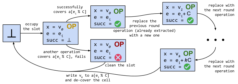
Figure 4. Life-cycle of the ops array slots, all transitions are performed by successful CAS-s. The states marked with ‘‘OP’’ store a descriptor reference, while the color specifies the status of this descriptor: ‘‘yellow’’ means ‘‘not defined yet’’, ‘‘red’’ --- ‘‘failed’’, and ‘‘green’’ -- ‘‘success’’.

Atomic EnqOp put.

Finally, we describe how to atomically change the descriptor status depending on whether the corresponding cell is covered. In our algorithm, we perform all such puts sequentially using the activeOp variable that defines the currently active EnqOp (line 26). To ensure lock-freedom, other threads can help modifying the status of the operation, and only the fastest among them succeeds. Hence, putOp function (lines 45--58) circularly goes through the ops slots, trying to find an empty one and to insert the current operation descriptor into it (line 49). At this point, the status of this EnqOp is not defined. Then the operation should be placed to activeOp via startPutOp, which tries to atomically change the field from $\bot$ to the descriptor (line 65) and helps other operations if needed (lines 61--64). Afterwards, the status of the operation is examined in tryPut method in EnqOp class --- it checks that the cell is not covered (lines 15--15) and the enqueues counter has not been changed (lines 19--20). At the end, activeOp is cleaned up (line 54) so other descriptors can be processed. If tryPut succeeds, putOp returns the corresponding slot number; otherwise, it cleans the slot (line 56) and returns -1.

A.1. Progress Guarantee

We prove lock-freedom of our bounded queue algorithm. We consider dequeue() and enqueue(..) operations separately.

The dequeue() operation.

Following the code, the only place where the operation can restart is an unsuccessful dequeues counter increment (line 33). However, each increment failure indicates that a concurrent dequeue() has successfully performed the same increment and completed. Lock-freedom for dequeues then trivially follows.

The enqueue(..) operation.

It is easy to notice that a successful enqueues counter increment indicates the system’s progress. This way, if we will show that the following assumption is incorrect: the counter is never changing and all the in-progress enqueues are stuck in a live-lock, we automatically show the enqueue(..) lock-freedom.

Let’s denote the current enqueues value, that cannot be changed, as $e_{\textit{stuck}}$. Our main idea is proving that there should appear a successful descriptor with field e equals $e_{\textit{stuck}}$. In this case, following the code, if the enqueues are stuck in a live-lock, there should exist an infinite number of restarts in enqueue(..) operations. By that these enqueue(..) operations should find the successful descriptor in ops array, if there exists one, and, thus, the counter enqueues should be incremented at some point. Thus, the assumption is correct only if a descriptor with successful field set to true cannot be put into ops.

Consider the function apply which is called by enqueue(..) operation (line 39). There are two possible scenarios: if findOp in line 77 finds a descriptor or not. Consider the first case. If it finds the descriptor $op$ with $op.e\geq e_{\textit{stuck}}$ then either we found the required descriptor or enqueues was incremented. Thus the found descriptor is from the previous round, the operation tries to replace it with a new one, already in the successful state (line 90). The corresponding CAS failure indicate that either the previous-round operation is completed and the slot becomes $\bot$, or a concurrent enqueue(..) successfully replaced the descriptor with a new one with op.e = $e_{\textit{stuck}}$. Since the second case breaks our assumption, we consider that the previous-round operation put $\bot$ into the slot, which leads to the second scenario, when we do not find the descriptor since the cell is not covered.

In the second case, findOp in apply function (line 77) did not find a descriptor and tries to put its own. Let’s assume now that each thread successfully finds and occupies an empty slot in a bounded number of steps in putOp function (lines 46--50). Thus, some descriptor with op.e = $e_{\textit{stuck}}$ should be successfully set into activeOp (see function startPutOp), and the following tryPut invocation sets the status to the successful one since there is no other successful descriptor that covers the cell according to the main assumption. This means, that the only way not to break this assumption is that is to never occupy a slot in putOp. However, since the ops size equals to the number of processes, the only way not to cover a slot during an array traversal, is that there exist an infinite amount of EnqOp descriptors which are put into ops. Obviously, e field on all of them is equal to $e_{\textit{stuck}}$ and at least one of them passes to activeOp and become successful by using the same argument as earlier.

As a result, we show that there should occur a successful descriptor with op.e = $e_{\textit{stuck}}$ in ops array in any possible scenario, which breaks the assumption and, thus, provides the lock-freedom guarantee for enqueue(..).

A.2. Correctness

This subsection is devoted for the linearizability proof of our algorithm. We split this subsection into two parts: the intuition of the proof and the full version.

A.2.1. Intuition

For dequeue(), lock-freedom guarantee is immediate, as the only case when the operation fails and has to retry is when the dequeues counter was concurrently incremented, which indicates that a concurrent dequeue() has made progress.

As for enqueue(..), all the CAS failures except for when the enqueues counter increments (line 40 in enqueue(..) and 72 in completeOp) or the ops slot occupation (line 49) fail intuitively indicate the system’s progress. In general, an enqueue(..) fails only due to helping, which does not cause retries. The only non-trivial situation is when a thread is stuck while trying to occupy a slot in putOp. Since the ops size equals the number of processes, it is guaranteed that when a thread intents to put an operation descriptor into ops, there is at least one free slot. Thus, if no slot can be taken during a traversal of ops, enqueues by other processes successfully take slots, and the system as a whole still makes progress.

The linearization points of the operations can be assigned as follows. A successful dequeue() operation linearizes at successful CAS in line 33. A failed dequeue() operation linearizes in line 29. For a successful enqueue(..) operation, we consider the descriptor op (created by that operation) that appears in ops array and has its successful field set. The linearization point of the operation is in CAS that changes enqueues counter from op.e to op.e + 1. A failed enqueue(..) operation linearizes in line 36. One can easily check that queue operations ordered according to their linearization points constitute a correct sequential history.

A.2.2. Full proof

At first, we suppose that all operations during execution are successful so the checks for emptiness and fullness never satisfy. This way, we are provided with an arbitrary finite history $H$, and we need to construct a linearization $S$ of $H$ by assigning a linearization point to each completed operation $\delta$ in $H$. We prove several lemmas before providing these linearization points.

Lemma A.1.

At any time during the whole execution, it is guaranteed that $\texttt{dequeues}\leq\texttt{enqueues}\leq\texttt{dequeues}+C$.

Proof.

We prove this by contradiction. Let dequeues exceed enqueues. Since the counters are always increased by one, we choose the first moment when dequeues becomes equal enqueues + 1 which, obviously, happens at the corresponding CAS invocation $\delta_{1}$ in dequeue() (line 33). Consider the situation right before this CAS $\delta_{1}$: enqueues and dequeues were equal. Consider the previous successful CAS $\delta_{0}$ that incremented enqueues or dequeues counter. Obviously, it was a CAS on dequeues since otherwise we chose not the first moment in the beginning of the proof. Thus, between $\delta_{0}$ and $\delta_{1}$ enqueues and dequeues did not change, and the emptiness check at line 32 should succeed during the dequeue() invocation that has performed $\delta_{1}$, so the CAS $\delta_{1}$ cannot be executed.

The situation when enqueues exceed dequeues + C can be shown to be unreachable in a similar manner. ∎

Further, we say that a descriptor EnqOp is successful if at some moment its successful field was set to true and it was in ops array.

Lemma A.2.

During the execution, for each value $pos\in[0,\texttt{enqueues}]$ there existed exactly one successful EnqOp object with the field e set to the specified $pos$.

Proof.

At first, we show that there exists at least one EnqOp descriptor. The enqueues counter can never increment if there does not exist the corresponding EnqOp object: CAS at line 40 is successful only if we put new object or the object exists, the same goes for line 72.

This object is unique, since we add objects EnqOp into array ops one by one using startPutOp function. In other words, the checks in Lines 15-20 are performed in the serialized manner. Thus, the object cannot become successful if it finds another object with the same value in field i in line 15. ∎

We denote the last EnqOp created by an enqueue(..) operation in line 39 as the last descriptor of the operation.

Lemma A.3.

The last descriptor of enq($x$) either becomes successful or the operation never finishes. Also, exactly one EnqOp descriptor created by the operation becomes successful.

Proof.

We note that if the descriptor does not become successful then the operation restarts at line 41. Note that the flag successful cannot be true at line 41 if the object was not added to ops array. Thus, it should become successful. ∎

Since by Lemma A.2 for each value $pos$ there exists exactly one EnqOp descriptor with the specified $pos$ and by Lemma A.3 enqueue(..) operation creates only one successful description, we can make a bijection between enqueue(..) operations and the positions $pos$: that are chosen as the value of the field e field in the last descriptor of the operation. (Note, that there is an obvious bijection between operations and descriptors.) Thus, we can say ‘‘the position of the enqueue’’ and ‘‘the enqueue of the position’’. Also, we say that EnqOp descriptor $op$ covers a cell $id$ if op.i = id.

The linearization points are defined straightforwardly. For deq() the linearization point is at the successful CAS performed in line 33. The linearization point for $\pi=\texttt{enq($x$)}$ is the successful CAS performed on enqueues counter in line 72 or line 40 from $E$ to $E+1$ where $E$ is the position of $\pi$.

Let $S_{\sigma}$ be the linearization of the prefix $\sigma$ of the execution $H$. Also, we map the state of our concurrent queue after the prefix $\sigma$ of $H$ to the state of the sequential queue $Q_{\sigma}$ provided by the algorithm in Figure 1. This map is defined as follows: the values of the counters enqueues and dequeues are taken as they are, and for each $pos\in[\texttt{dequeues},\texttt{enqueues})$ the value in the position $pos$ % C contains $op.x$ of successful EnqOp $op$ with $op.e=pos$ from ops array or, if such $op$ does not exist, simply a[$pos$ % C].

Lemma A.4.

The sequential history $S_{H}$ complies with the queue specification.

Proof.

We use induction on $\sigma$ to show that for every prefix $\sigma$ of $H$, $S_{\sigma}$ is a queue history and the state of the sequential queue $L_{\sigma}$ from Figure 1 after executing $S_{\sigma}$ is equal to $Q_{\sigma}$. The claim is clearly true for $\sigma=\epsilon$. For the inductive step we have $\sigma=\sigma_{1}\circ\delta$ and $L_{\sigma_{1}}$ after $S_{\sigma_{1}}$ coincides with $Q_{\sigma_{1}}$.

Suppose, $\delta$ is the successful CAS in line 33 of operation $\pi=\texttt{deq()}$. Consider the last two reads d := dequeues, $\delta_{1}$, and e := enqueues, $\delta_{2}$, in Line 29 in $\pi$. Suppose that $\delta_{1}$ reads $D$ as d and $\delta_{2}$ reads $E$ as e. Let $\sigma_{2}$ be the prefix of $H$ that ends on $\delta_{2}$. Since we forbid $\pi$ to satisfy the emptyness property we could totally say that the linearization point of the enqueue(..) of position $D$ already passed since $E>D$, otherwise, $\pi$ should have been restarted in line 31. Thus, by induction $Q_{\sigma_{2}}$ and $L_{\sigma_{2}}$ both contains same $v$ at position d % C. The same holds for $Q_{\sigma_{1}}$ and $L_{\sigma_{1}}$. Thus, between $\delta_{2}$ and $\delta$ queue $Q$ always contains $v$ in d % C such as queue $L$. By the definition of $Q$ this means during that interval there is always exist either successful EnqOp $op$ with $op.e=D$ and $op.x=v$ or $v$ is stored in a[$D$ % C], thus readElem(d % C) in line 30 would correctly read $v$. This means, that the result of deq() in both, the concurrent and the sequential, queues coincides.

Suppose, $\delta$ is the successful CAS in line 40 of operation $\pi=\texttt{enq($v$)}$. Suppose that during e := enqueues in line 36, $\delta_{1}$, we read $E$. We want to prove that three things: 1) there already existed successful EnqOp $op$ with $op.e=E$; 2) there is no EnqOp $op$ with op.e < $E$ and op.i = $E$ % C in ops array; and 3) none of EnqOp descriptor $op_{2}$ with $op_{2}$.e > $E$ and $op_{2}$.i = $E$ % C exist before $\delta$. It will be enough since by our mapping the cell $E$ % C will contain the same value in both queues $Q_{\sigma}$ and $L_{\sigma}$, because if there is no successful descriptor $op$ in ops with op.e = $E$ then it already dumps its value to array a in line 71 and nobody could have overwritten in.

Note, that the second and the third part can be proved very simply. As for the second part, if we find an outdated descriptor with the same i we replace it to the new one in line 90. As for the third part, since enqueues does not exceed $E$ before $\delta$, then no process can even create EnqOp descriptor $op$ with op.e > $E$.

This means, that we are left to prove the first part. Since the CAS in line 40, $\delta$, is successful then enqueues counter did not change in-between $\delta_{1}$ and $\delta$. Thus, during apply operation in line 39 enqueues was constant. Let us look on what this operation is doing. At first, it tries to find a successful descriptor EnqOp $op$ for which $op=E$ % C in line 77. If it does not exist (the check in line 79 succeeds) it tries to put its own descriptor by using the function putOp in line 80. As the first step, it tries to put not yet successful EnqOp $op$ into array ops (line 49). The operation did not become successful in tryPut() function only if either there exists EnqOp $op$ with $op=E$ % C or enqueues changes. Since, enqueues cannot change as we discussed prior, thus in line 15 finds EnqOp $op$ with $op.i=E$ % C. Note that since enqueues did not change and findOp in line 77 did not find an operation, then $op.e$ has to be equal to $E$, thus, providing with what we desired. In the other case, apply finds EnqOp $op$ with $op.i=E$ % C. Note that since enqueues does not change $op.i$ cannot exceed $e$. Thus, if the check in line 85 succeeds, $op.e$ should be equal to $E$ and we are done. Otherwise, this means that we found some old $op$ and we try to replace it by CAS in line 90. Due to the fact that enqueues does not change, CAS can fail only if another EnqOp descriptor $op$ with $op.e=E$ is successfully placed. By that, there existed EnqOp object that we desired. Thus, after we add $\delta$ to $\sigma_{1}$, $Q_{\sigma}$ and $L_{\sigma}$ coincides.

Suppose, $\delta$ is the successful CAS in line 72 of operation $\pi=\texttt{enq($v$)}$. As in the previous case, it is enough to prove two things: 1) there already exists corresponding EnqOp; 2) there are no other EnqOp that cover the same cell in ops array. The second statement is easy to prove as before. For the first one, we note that we apply $\delta$ only if we find a successful descriptor by readOp(opSlot) in line 70.

Finally, suppose that $\delta$ is none of the successful CAS in Lines 33, 40 and 72. Thus, $L_{\sigma}$ does not change between $\sigma_{1}$ and $\sigma$. At the same time, $Q_{\sigma}$ can change only due to the removal of EnqOp descriptor from array ops. This can happen in two places: successful CAS operations in line 90 and in line 73. In the first case, nothing happens since we simply replace old EnqOp descriptor with the new one, thus $Q_{\sigma}$ remains the same. In the second case, the successful CAS means that no new descriptor is stored in array ops with the same value in field i and enqueues does not yet come to the next round, otherwise, $op$ read in line 70 should have been replaced by 90. Thus, the value stored in array a is exactly what was stored by $op$ until dequeues passes through that position. ∎

Note that the proof of the previous lemma is enough to show that the implementation is linearizable if we throw away operations for which check for emptiness or fullness is satisfied. However, such operations are very easy to linearize. Unsuccessful deq() is linearized at line 29 while unsuccessful enq($v$) is linearized at line 36. Note that the correctness of the choice of the linearization points can be proved the same way as above, since enqueues and dequeues counters of $Q_{\sigma}$ matchenqueues and dequeues counters of $L_{\sigma}$.