Linear Convergence of the Subspace Constrained Mean Shift Algorithm: From Euclidean to Directional Data

Abstract

This paper studies the linear convergence of the subspace constrained mean shift (SCMS) algorithm, a well-known algorithm for identifying a density ridge defined by a kernel density estimator. By arguing that the SCMS algorithm is a special variant of a subspace constrained gradient ascent (SCGA) algorithm with an adaptive step size, we derive the linear convergence of such SCGA algorithm. While the existing research focuses mainly on density ridges in the Euclidean space, we generalize density ridges and the SCMS algorithm to directional data. In particular, we establish the stability theorem of density ridges with directional data and prove the linear convergence of our proposed directional SCMS algorithm.

and

1 Introduction

Identifying meaningful lower dimensional structures from a point cloud has long been a popular research topic in Statistics and Machine Learning (Izenman, 2012; Wasserman, 2018). One reliable characterization of such a low-dimensional structure is the density ridge, which can be feasibly estimated by a kernel density estimator (KDE) from point cloud data (Eberly, 1996; Genovese et al., 2014). Loosely speaking, an estimated density ridge signifies a high-density curve or surface in a point cloud; see the left panel of Figure 1. Let $p$ be the underlying probability density function that generates the data in the Euclidean space $\mathbb{R}^{D}$. Its order-$d$ density ridge $R_{d}$ with $0\leq d<D$ is the set of points defined as:

$$R_{d}=\left\{\bm{x}\in\mathbb{R}^{D}:V_{d}(\bm{x})^{T}\nabla p(\bm{x})=\bm{0},\lambda_{d+1}(\bm{x})<0\right\},$$ (1)

where $\lambda_{1}(\bm{x})\geq\cdots\geq\lambda_{D}(\bm{x})$ are the eigenvalues of Hessian $\nabla\nabla p(\bm{x})$ and $V_{d}(\bm{x})\in\mathbb{R}^{D\times(D-d)}$ has its columns as the last $D-d$ orthonormal eigenvectors. The notion of density ridges has appeared in various scientific fields, such as medical imaging (You et al., 2011), seismology (Sasaki et al., 2017), and astronomy (Sousbie et al., 2007; Chen et al., 2016). To locate an estimated density ridge defined by (Euclidean) KDE, Ozertem and Erdogmus (2011) proposed a practical method called subspace constrained mean shift (SCMS) algorithm.

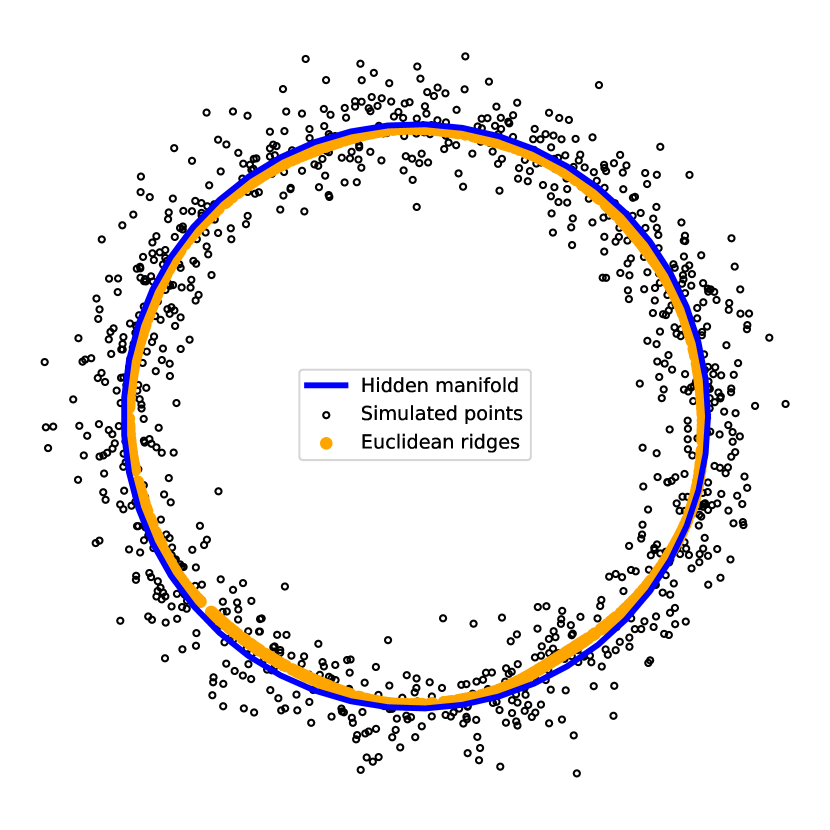
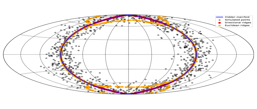
Figure 1: Density ridges estimated by Euclidean and directional SCMS algorithms on two synthetic datasets (drawn as black points) with hidden circular manifold structures (indicated by blue curves) on $\mathbb{R}^{2}$ and the unit sphere $\Omega_{2}\subset\mathbb{R}^{3}$, respectively. Left: The orange points indicate the estimated ridge obtained by the Euclidean SCMS algorithm from the dataset on $\mathbb{R}^{2}$. Right: The red points represent the estimated directional ridge identified by our directional SCMS algorithm, while the orange points indicate the estimated ridge obtained by the Euclidean SCMS algorithm from the dataset on $\Omega_{2}$. This panel is presented under the Hammer projection; see Appendix B for more details.

While the statistical estimation and asymptotic theories of density ridges in $\mathbb{R}^{D}$ have been well-studied (Genovese et al., 2014; Chen et al., 2015; Qiao and Polonik, 2016; Chen et al., 2015a; Qiao, 2021), the literature falls short of addressing the algorithmic properties of the ridge-finding method, i.e., the SCMS algorithm. To the extent of our knowledge, Ghassabeh et al. (2013); Ghassabeh and Rudzicz (2020) were the only available works to investigate the SCMS algorithm and its modified version from an algorithmic perspective. However, they only proved a non-decreasing property of density estimates and the validity of two stopping criteria for the SCMS algorithm. The algorithmic convergence of the SCMS algorithm remains an open question. There are two challenges to answering this question. First, because every iteration of the SCMS algorithm involves a projection matrix defined by the (estimated) Hessian, it is no longer a conventional first-order method in optimization. Second, estimating a density ridge in practice is a nonconvex/nonconcave optimization problem. Thus, the first objective of this paper is to provide a theoretical study on the algorithmic convergence and its associated (linear) rate of convergence for the SCMS algorithm.

In stark contrast to abundant research papers about density ridges in the Euclidean space, little work has been done to examine the statistical properties and any practical algorithm of estimating density ridges on the unit hypersphere $\Omega_{q}=\{\bm{x}\in\mathbb{R}^{q+1}:\|\bm{x}\|_{2}=1\}\subset\mathbb{R}^{q+1}$. Nevertheless, data on $\Omega_{q}$ are ubiquitous in many scientific fields of study, such as seismology (e.g., longitudes and latitudes of the epicenters of earthquakes) and astronomy (e.g., right ascensions and declinations of astronomical objects). Such data are generally known as directional data in the statistical literature (Mardia and Jupp, 2000; Ley and Verdebout, 2017). Hence, the second objective of this paper is to generalize density ridges and the SCMS algorithm to directional data.

More importantly, identifying an estimated density ridge from directional data on $\Omega_{2}$ by the Euclidean SCMS algorithm always suffers from high bias near the two poles of $\Omega_{2}$. Consider a synthetic dataset with independently and identically distributed (i.i.d.) observations $\left\{\bm{X}_{1},...,\bm{X}_{1000}\right\}$ from a great circle connecting the North and South Poles of $\Omega_{2}$ with additive noises. We apply both the Euclidean and directional SCMS algorithms to this simulated dataset. While the estimated ridges by the Euclidean SCMS algorithm fail to recover the desired great circle in high latitude regions, the ridges identified by our proposed directional SCMS algorithm align well with the underlying circular structure; see the right panel in Figure 1 for a preview and Appendix B for a more detailed discussion.

Main Results. The main contributions of this paper are summarized as follows:

$\bullet$ We present the convergence analysis of the SCMS and the general SCGA algorithms and prove their linear convergence properties with Euclidean data (Theorem 3.6, Corollary 3.7, and related discussion in Section 3.3):

$$\left|\left|\widehat{\bm{x}}^{(t)}-\widehat{\bm{x}}^{*}\right|\right|_{2}\leq\Upsilon^{t}\left|\left|\widehat{\bm{x}}^{(0)}-\widehat{\bm{x}}^{*}\right|\right|_{2},$$

where $\big{\{}\widehat{\bm{x}}^{(t)}\big{\}}_{t=0}^{\infty}$ is a sequence of points generated by the SCGA or SCMS algorithm in $\mathbb{R}^{D}$, $\widehat{\bm{x}}^{*}$ is the limit point of the sequence, and $0<\Upsilon<1$ is a constant.

$\bullet$ We generalize density ridges and the SCMS algorithm to directional data on $\Omega_{q}$ (Section 4).

$\bullet$ We prove the statistical convergence rate of a ridge estimator on the sphere $\Omega_{q}$ defined by the directional KDE (Theorem 4.1):

$$\mathtt{Haus}(\underline{R}_{d},\underline{\widehat{R}}_{d})=O\left(h^{2}\right)+O_{P}\left(\sqrt{\frac{|\log h|}{nh^{q+4}}}\right),$$

where $\underline{R}_{d}$ and $\underline{\widehat{R}}_{d}$ are the population and estimated directional density ridges, respectively, $\mathtt{Haus}$ is the Hausdorff distance, and $q$ is the dimension of $\Omega_{q}$.

$\bullet$ We establish the convergence of the SCMS and the general SCGA algorithms with directional data and derive their linear convergence results (Theorem 4.6, Corollary 4.7, and related expositions in Section 4.3):

$$d_{g}(\widehat{\underline{\bm{x}}}^{(t)},\widehat{\underline{\bm{x}}}^{*})\leq\underline{\Upsilon}^{t}\cdot d_{g}(\widehat{\underline{\bm{x}}}^{(0)},\widehat{\underline{\bm{x}}}^{*}),$$

where $\big{\{}\widehat{\underline{\bm{x}}}^{(t)}\big{\}}_{t=0}^{\infty}$ is the sequence of points generated by the directional SCGA or SCMS algorithm, $\widehat{\underline{\bm{x}}}^{*}$ is the convergence point, $0<\underline{\Upsilon}<1$ is a constant, and $d_{g}$ is the geodesic distance on $\Omega_{q}$.

Other Related Literature. The problem of density ridge estimation has its unique standing in both the computer science and statistics literature; see Hall et al. (1992); Eberly (1996); Damon (1999); Hall et al. (2001) and references therein. Among various definition of density ridges (Norgard and Bremer, 2012; Peikert et al., 2013), our definition follows from Eberly (1996); Genovese et al. (2014); Chen et al. (2015), because its statistical estimation theory has been well-established and it is feasible to be directly generalized to directional densities. Practically, the SCMS algorithm for identifying an estimated density ridge first appeared in the field of computer vision (Saragih et al., 2009) before its introduction to the statistical community by Ozertem and Erdogmus (2011). More recently, Qiao and Polonik (2021) proposed alternative methods to the SCMS algorithm for finding density ridges, which are based on a gradient descent of the ridgeness and have connections to solution manifolds (Chen, 2020). They presented the convergence analysis on continuous versions of their proposed methods and discretized them via Euler’s method. Our directional SCMS algorithm is extended from the directional mean shift algorithm (Oba et al., 2005; Kafai et al., 2010; Kobayashi and Otsu, 2010; Yang et al., 2014; Zhang and Chen, 2021a, b). As we cast the (directional) SCMS algorithms into subspace constrained gradient ascent (SCGA) algorithms (on a hypersphere), it is worth mentioning that one should not confuse the SCGA algorithm here with the projected gradient ascent/descent method for a constrained problem in the standard optimization theory; see Section 3.2 in Bubeck (2015) for some references of the latter one. The SCGA algorithm discussed in this paper is a gradient ascent algorithm but with a subspace constrained gradient. When the subspace coincides with alternating one-dimensional coordinate spaces, the SCGA algorithm reduces to the well-known coordinate ascent/descent method (Wright, 2015). Some linear convergence results of the coordinate descent algorithms were previously established by Luo and Tseng (1992); Beck and Tetruashvili (2013). Other related work includes Kozak et al. (2019, 2020), though, in their problem setups, the projection matrix onto the subspace is random and has its expectation equal to the identity matrix. Our interested SCGA algorithm always has a deterministic constrained subspace defined by the eigenspace associated with the last several eigenvalues of the Hessian of the density $p$.

Outlines and Notations. Section 2 introduces the definitions of Euclidean and directional KDEs and reviews some preliminary concepts of differential geometry on $\Omega_{q}$. We discuss the assumptions on the Euclidean density ridges and establish the (linear) convergence results of the SCGA and SCMS algorithms in Section 3. In Section 4, we generalize the definition of density ridges to the directional data scenario and prove the (linear) convergence properties of the SCGA and SCMS algorithms on $\Omega_{q}$. Some simulation studies and real-world applications of Euclidean and directional SCMS algorithms are presented in Section 5, whose code is available at https://github.com/zhangyk8/EuDirSCMS. We conclude the paper and discuss some potential impacts in Section 6.

Throughout the paper we use $d$ as the intrinsic dimension of density ridges, whose ambient spaces are $\mathbb{R}^{D}$ in the Euclidean data case and $\Omega_{q}=\left\{\bm{x}\in\mathbb{R}^{q+1}:\left|\left|\bm{x}\right|\right|_{2}=1\right\}$ in the directional data case. Notice that a quantity under the directional data setting that has its counterpart in the Euclidean data case will be denoted by the same notation with an extra underline. For instance, $R_{d}$ is a ridge of the density $p$ in the Euclidean space $\mathbb{R}^{D}$ while $\underline{R}_{d}$ refers to a ridge of the directional density $f$ on the sphere $\Omega_{q}$.

Let $f:\mathbb{R}^{D}\to\mathbb{R}$ be a smooth function and $[\alpha]=(\alpha_{1},...,\alpha_{D})$ be a multi-index (that is, $\alpha_{1},...,\alpha_{D}$ are nonnegative integers and $|[\alpha]|=\sum_{i=1}^{D}\alpha_{i}$). Define $D^{[\alpha]}=\frac{\partial^{\alpha_{1}}}{\partial x_{1}^{\alpha_{1}}}\cdots\frac{\partial^{\alpha_{D}}}{\partial x_{D}^{\alpha_{D}}}$ as the $|[\alpha]|$-th order partial derivative operator, where $D^{[\alpha]}f$ is often written as $f^{(\alpha)}$. For $j=0,1,...$, we define the functional norms

$$\left|\left|f\right|\right|_{\infty}^{(j)}=\max_{\alpha:|[\alpha]|=j}\sup_{\bm{x}\in\mathbb{R}^{D}}|f^{(\alpha)}(\bm{x})|.$$

When $j=0$, this becomes the infinity norm of $f$; for $j>0$, the above norms are indeed some semi-norms. We also define $\left|\left|f\right|\right|_{\infty,k}^{*}=\max_{j=0,...,k}\left|\left|f\right|\right|_{\infty}^{(j)}$.

The (total) gradient and Hessian of $f$ are defined as $\nabla f(\bm{x})=\Big{(}\frac{\partial f(\bm{x})}{\partial x_{1}},...,\frac{\partial f(\bm{x})}{\partial x_{D}}\Big{)}^{T}$ and $\nabla\nabla f(\bm{x})=\Big{(}\frac{\partial^{2}f(\bm{x})}{\partial x_{i}\partial x_{j}}\Big{)}_{1\leq i,j\leq D}$. Inductively, the third derivative of $f(\bm{x})$ is a $D\times D\times D$ array given by $\nabla^{3}f(\bm{x})=\Big{(}\frac{\partial^{3}}{\partial x_{i}\partial x_{j}\partial x_{k}}f(\bm{x})\Big{)}_{1\leq i,j,k\leq D}$. When $f$ is a directional density supported on $\Omega_{q}$, the preceding functional norms are defined via the Riemannian gradient, Hessian, and high-order derivatives of $f(\bm{x})$ within the tangent space $T_{\bm{x}}$ at $\bm{x}\in\Omega_{q}$, and the supremum will be taken over $\Omega_{q}$ instead of $\mathbb{R}^{D}$. They are equivalent to the derivatives of $f$ with respect to the local coordinate chart on $\Omega_{q}$; see Section 2.3 for a review.

Let $A_{jk}$ denote the $(j,k)$ entry of a matrix $A\in\mathbb{R}^{m\times n}$. Then, the Frobenius norm is $\left|\left|A\right|\right|_{F}=\sqrt{\sum_{j,k}A_{jk}^{2}}=\mathtt{tr}(A^{T}A)$, where $\mathtt{tr}(A^{T}A)$ is the trace of the square matrix $A^{T}A$, and the operator norm is $\left|\left|A\right|\right|=\sup_{||\bm{x}||=1}\left|\left|A\bm{x}\right|\right|$. In most cases, we consider the $L_{2}$ (operator) norm $\left|\left|\cdot\right|\right|_{2}$. We define $\left|\left|A\right|\right|_{\max}=\max_{j,k}|A_{jk}|$. The inequality relationships between the above matrix norms are $\left|\left|A\right|\right|_{2}\leq\left|\left|A\right|\right|_{F}\leq\sqrt{n}\left|\left|A\right|\right|_{2}$, $\left|\left|A\right|\right|_{\max}\leq\left|\left|A\right|\right|_{2}\leq\sqrt{mn}\left|\left|A\right|\right|_{\max}$, and $\left|\left|A\right|\right|_{F}\leq\sqrt{mn}\left|\left|A\right|\right|_{\max}$.

We use the big-O notation $h(\bm{x})=O(g(\bm{x}))$ if the absolute value of $h(\bm{x})$ is upper bounded by a positive constant multiple of $g(\bm{x})$ for all sufficiently large $\bm{x}$. In contrast, $h(\bm{x})=o(g(\bm{x}))$ when $\lim_{\left|\left|\bm{x}\right|\right|_{2}\to\infty}\frac{|h(\bm{x})|}{g(\bm{x})}=0$. For random vectors, the notation $o_{P}(1)$ is short for a sequence of random vectors that converges to zero in probability. The expression $O_{P}(1)$ denotes the sequence that is bounded in probability; see Section 2.2 of van der Vaart (1998) for details.

2 Preliminaries

In this section, we review the KDE with Euclidean and directional data as well as some differential geometry concepts on $\Omega_{q}$.

2.1 Kernel Density Estimation with Euclidean Data

Let $\{\bm{X}_{1},...,\bm{X}_{n}\}$ be a random sample from a distribution $P$ with density $p$ supported on the Euclidean space $\mathbb{R}^{D}$. We call such random sample $\{\bm{X}_{1},...,\bm{X}_{n}\}$ Euclidean data in the sequel. The (Euclidean) KDE at point $\bm{x}\in\mathbb{R}^{D}$ with a kernel function $K$ and bandwidth parameter $h\equiv h(n)$ is written as (Wasserman, 2006; Scott, 2015; Chen, 2017):

$$\widehat{p}_{n}(\bm{x})=\frac{1}{nh^{D}}\sum_{i=1}^{n}K\left(\frac{\bm{x}-\bm{X}_{i}}{h}\right).$$ (2)

The kernel $K:\mathbb{R}^{D}\to\mathbb{R}$ is generally a unimodal function satisfying the following properties:

• (K1) $\int_{\mathbb{R}^{D}}K(\bm{x})d\bm{x}=1$.

• (K2) $K(\bm{x})$ is (radially) symmetric, i.e., $\int_{\mathbb{R}^{D}}\bm{x}\,K(\bm{x})\,d\bm{x}=0$.

• (K3) $\lim\limits_{\left|\left|\bm{x}\right|\right|_{2}\to\infty}\left|\left|\bm{x}\right|\right|_{2}^{D}K(\bm{x})=0$ and $\int_{\mathbb{R}^{D}}\left|\left|\bm{x}\right|\right|_{2}^{2}K(\bm{x})d\bm{x}<\infty$, where $\left|\left|\cdot\right|\right|_{2}$ is the usual $L_{2}$ norm in $\mathbb{R}^{D}$.

One possible approach to construct a multivariate kernel $K(\bm{x})$ with the above properties is to derive it from a kernel profile as follows:

$$K(\bm{x})=c_{k,D}\cdot k\left(\left|\left|\bm{x}\right|\right|_{2}^{2}\right),$$ (3)

where $c_{k,D}$ is the normalizing constant such that $K$ satisfies (K1) and the function $k:[0,\infty)\to[0,\infty)$ is called the profile of the kernel. This kernel form is generally used in deriving (subspace constrained) mean shift algorithms; see Section 3.2. An important example of the profile function is $k_{N}(x)=\exp\left(-\frac{x}{2}\right)$ for $x\geq 0$, leading to the multivariate Gaussian kernel $K_{N}(\bm{x})=\frac{1}{(2\pi)^{\frac{D}{2}}}\exp\left(-\frac{\left|\left|\bm{x}\right|\right|_{2}^{2}}{2}\right)$.

Another approach of designing a multivariate kernel function is to leverage the product kernel technique as $K(\bm{x})=K_{1}(x_{1})\cdots K_{D}(x_{D})$, where $K_{1},...,K_{D}$ are kernels function defined on $\mathbb{R}$ satisfying the properties (K1-3). This leads to a multivariate KDE as:

$$\widehat{p}_{n}(\bm{x})=\frac{1}{nh^{D}}\sum_{i=1}^{n}K_{1}\left(\frac{x_{1}-X_{i,1}}{h}\right)\cdots K_{D}\left(\frac{x_{D}-X_{i,D}}{h}\right).$$ (4)

In fact, the multivariate Gaussian kernel $K_{N}$ can be obtained by defining its kernel profile as $k_{N}(x)=\exp\left(-\frac{x}{2}\right)$ for $x\geq 0$ or taking $K_{1}(x)=\cdots=K_{D}(x)=\frac{1}{\sqrt{2\pi}}\exp\left(-\frac{x^{2}}{2}\right)$. In practice, the multivariate KDE (2) with Gaussian kernel is the most popular nonparametric density estimator with Euclidean data.

The most crucial part in applying the KDE is to select the bandwidth parameter $h$. Common methods in the literature aim at minimizing the mean integrated square error (MISE):

$$\text{MISE}=\mathbb{E}\int_{\mathbb{R}^{D}}\left[\widehat{p}_{n}(\bm{x})-p(\bm{x})\right]^{2}d\bm{x}$$

or its asymptotic part through the rule of thumb (Silverman, 1986), cross validation (Rudemo, 1982; Bowman, 1984; Hall, 1983; Stone, 1984), and plug-in methods (Sheather and Jones, 1991). As choosing the bandwidth is not the main focus of this paper, we refer the interested reader to Jones et al. (1996); Sheather (2004) and Chapter 6.5 of Scott (2015) for comprehensive reviews.

2.2 Kernel Density Estimation with Directional Data

The Euclidean KDE (2) exhibits some salient drawbacks in dealing with directional data samples; see Appendix B for a detailed exposition. Fortunately, the theory of kernel density estimation with directional data has been well-studied since late 1970s (Beran, 1979; Hall et al., 1987; Bai et al., 1988; Zhao and Wu, 2001; García-Portugués, 2013; Pewsey and García-Portugués, 2021). Let $\bm{X}_{1},...,\bm{X}_{n}\in\Omega_{q}\subset\mathbb{R}^{q+1}$ be a random sample generated from an underlying directional density function $f$ on $\Omega_{q}$ with $\int_{\Omega_{q}}f(\bm{x})\,\omega_{q}(d\bm{x})=1,$ where $\omega_{q}$ is the Lebesgue measure on $\Omega_{q}$. The directional KDE is given by:

$$\widehat{f}_{h}(\bm{x})=\frac{c_{L,q}(h)}{n}\sum_{i=1}^{n}L\left(\frac{1-\bm{x}^{T}\bm{X}_{i}}{h^{2}}\right)=\frac{c_{L,q}(h)}{n}\sum_{i=1}^{n}L\left(\frac{1}{2}\left|\left|\frac{\bm{x}-\bm{X}_{i}}{h}\right|\right|_{2}^{2}\right),$$ (5)

where $L$ is a directional kernel (i.e., a rapidly decaying function with nonnegative values and defined on $(-\delta_{L},\infty)\subset\mathbb{R}$ for some constant $\delta_{L}>0$), $h>0$ is the bandwidth parameter, and $c_{L,q}(h)$ is a normalizing constant satisfying $c_{L,q}(h)^{-1}=\int_{\Omega_{q}}L\left(\frac{1-\bm{x}^{T}\bm{y}}{h^{2}}\right)\omega_{q}(d\bm{y})=O(h^{q})$.

Remark 2.1.

The distance metric used by the directional KDE (5) on $\Omega_{q}$ is identical to the standard Euclidean metric in the ambient space $\mathbb{R}^{q+1}$. This is because the standard Euclidean metric $\left|\left|\cdot\right|\right|_{2}$ of $\mathbb{R}^{q+1}$ is topologically equivalent (but not strongly equivalent) to the geodesic distance $d_{g}(\cdot,\cdot)$ on $\Omega_{q}$ due to the following equality:

$$\left|\left|\bm{x}-\bm{y}\right|\right|_{2}=2\sin\left(\frac{d_{g}(\bm{x},\bm{y})}{2}\right).$$ (6)

See Section C.1.5 in Ok (2007) for the definition of equivalence of metrics. Hence, the distance metric in (5) is indeed intrinsic on $\Omega_{q}$ and adaptive to its geometry.

As in the applications of Euclidean KDEs, the bandwidth selection is a critical part in determining the performances of directional KDEs (Hall et al., 1987; Bai et al., 1988; Taylor, 2008; Marzio et al., 2011; Oliveira et al., 2012; García-Portugués, 2013; Saavedra-Nieves and María Crujeiras, 2020). On the contrary, the choice of the kernel is less crucial; see, e.g., Page 72 of Wasserman (2006) and Section 6.3.2 in Scott (2015) for the reasoning. A popular candidate is the so-called von Mises kernel $L(r)=e^{-r}$, which serves as a counterpart of the Gaussian kernel for directional KDEs. Its name originates from the famous $q$-von Mises-Fisher distribution on $\Omega_{q}$, which is denoted by $\text{vMF}(\bm{\mu},\nu)$ and has the density as:

$$f_{\text{vMF}}(\bm{x};\bm{\mu},\nu)=C_{q}(\nu)\cdot\exp(\nu\bm{\mu}^{T}\bm{x})\quad\text{ with }\quad C_{q}(\nu)=\frac{\nu^{\frac{q-1}{2}}}{(2\pi)^{\frac{q+1}{2}}\mathcal{I}_{\frac{q-1}{2}}(\nu)},$$ (7)

where $\bm{\mu}\in\Omega_{q}$ is the directional mean, $\nu\geq 0$ is the concentration parameter, and $\mathcal{I}_{\alpha}(\nu)$ is the modified Bessel function of the first kind at order $\nu$. For more details on statistical properties of the von Mises-Fisher distribution and directional KDE, we refer the interested reader to Mardia and Jupp (2000); Banerjee et al. (2005); García-Portugués et al. (2013).

2.3 Riemannian Gradient, Hessian, and Exponential Map on $\Omega_{q}$

Given that the unit hypersphere $\Omega_{q}$ is a nonlinear manifold, the Riemannian gradient and Hessian of a smooth function $f$ on $\Omega_{q}$ are defined within its tangent spaces. They are different from but also interconnected with the total gradient and Hessian of $f$ in the ambient Euclidean space $\mathbb{R}^{q+1}$.

$\bullet$ Riemannian Gradient on $\Omega_{q}$. Let $T_{\bm{x}}$ be the tangent space of $\Omega_{q}$ at point $\bm{x}\in\Omega_{q}$, which consists of all the vectors starting from $\bm{x}$ and tangent to $\Omega_{q}$. Given a smooth function $f:\Omega_{q}\to\mathbb{R}$, its Riemannian gradient $\mathtt{grad}\,f(\bm{x})\in T_{\bm{x}}$ is defined as:

$$\left\langle\bm{v},\mathtt{grad}\,f(\bm{x})\right\rangle_{\bm{x}}=df_{\bm{x}}(\bm{v})$$ (8)

for any (unit) vector $\bm{v}\in T_{\bm{x}}$, where $\langle\cdot,\cdot\rangle_{\bm{x}}$ is the inner product (or Riemannian metric) in $T_{\bm{x}}$ and $df_{\bm{x}}:T_{\bm{x}}\to\mathbb{R}$ is the differential operator of $f$ at $\bm{x}\in\Omega_{q}$; see, e.g., Section 3.1 in Banyaga and Hurtubise (2004) for more details. Note that the Riemannian metric on $\Omega_{q}$ coincides with the standard inner product $\langle\cdot,\cdot\rangle$ in the ambient space $\mathbb{R}^{q+1}$; see Section 3.6.1 in Absil et al. (2008). If $f$ is smooth in an open neighborhood containing $\Omega_{q}$ and we consider $\mathtt{grad}\,f(\bm{x}),\bm{v}\in T_{\bm{x}}$ as vectors in $\mathbb{R}^{q+1}$, then the inner product in $T_{\bm{x}}$ reduces to the usual one in $\mathbb{R}^{q+1}$ and the Riemannian gradient $\mathtt{grad}\,f(\bm{x})$ can be expressed in terms of the total gradient $\nabla f(\bm{x})$ as:

$$\mathtt{grad}\,f(\bm{x})=\left(\bm{I}_{q+1}-\bm{x}\bm{x}^{T}\right)\nabla f(\bm{x}),$$ (9)

where $\bm{I}_{q+1}\in\mathbb{R}^{(q+1)\times(q+1)}$ is the identity matrix. The left-hand side of (9) is the projection of the total gradient $\nabla f(\bm{x})$ onto the tangent space $T_{\bm{x}}$ at $\bm{x}\in\Omega_{q}$.

$\bullet$ Riemannian Hessian on $\Omega_{q}$. The Riemannian Hessian $\mathcal{H}f(\bm{x})$ at point $\bm{x}\in\Omega_{q}$ is a symmetric bilinear map from the tangent space $T_{\bm{x}}$ into itself defined as:

$$\mathcal{H}f(\bm{x})\left[\bm{v}\right]=\bar{\nabla}_{\bm{v}}\mathtt{grad}\,f(\bm{x})$$ (10)

for any $\bm{v}\in T_{\bm{x}}$, where $\bar{\nabla}_{\bm{v}}$ is the Riemannian connection on $\Omega_{q}$. Similar to $\mathtt{grad}\,f(\bm{x})$, the Riemannian Hessian $\mathcal{H}f(\bm{x})$ has the following explicit formula when viewed in the ambient Euclidean space $\mathbb{R}^{q+1}$:

$$\mathcal{H}f(\bm{x})=(\bm{I}_{q+1}-\bm{x}\bm{x}^{T})\left[\nabla\nabla f(\bm{x})-\nabla f(\bm{x})^{T}\bm{x}\cdot\bm{I}_{q+1}\right](\bm{I}_{q+1}-\bm{x}\bm{x}^{T}),$$ (11)

where $\nabla f(\bm{x})$ and $\nabla\nabla f(\bm{x})$ are the total gradient and Hessian of $f$ in $\mathbb{R}^{q+1}$. This formula can be derived via the Riemannian connection and Weingarten map on $\Omega_{q}$ (Absil et al. 2013 and Section 5.5 in Absil et al. 2008) or geodesics on $\Omega_{q}$ (Zhang and Chen, 2021a).

$\bullet$ Exponential Map. An exponential map $\mathtt{Exp}_{\bm{x}}:T_{\bm{x}}\to\Omega_{q}$ at $\bm{x}\in\Omega_{q}$ is a mapping that takes a vector $\bm{v}\in T_{\bm{x}}$ to a point $\bm{y}:=\mathtt{Exp}_{\bm{x}}(\bm{v})\in\Omega_{q}$ along the curve $\varphi$ with $\varphi(0)=\bm{x},\varphi(1)=\bm{y}$ and $\varphi^{\prime}(0)=\bm{v}$. Here, $\varphi:[0,1]\to\Omega_{q}$ is a curve of minimum length between $\bm{x}$ and $\bm{y}$ (i.e., the so-called geodesic on $\Omega_{q}$). An intuitive way of thinking of the exponential map $\mathtt{Exp}_{\bm{x}}$ evaluated at $\bm{v}$ on $\Omega_{q}$ is that starting at point $\bm{x}$, we identify another point $\bm{y}$ on $\Omega_{q}$ along the geodesic (or great circle) in the direction of $\bm{v}$ so that the geodesic distance between $\bm{x}$ and $\bm{y}$ is $\left|\left|\bm{v}\right|\right|_{2}$. As $\Omega_{q}$ is a compact Riemannian manifold, the exponential map $\mathtt{Exp}_{\bm{x}}$ is a diffeomorphism (smooth bijection) from a neighborhood of $\bm{0}\in T_{\bm{x}}$ to its image on $\Omega_{q}$; see Lemma 6.16 in Lee (2018). The inverse of an exponential map (or logarithmic map) is defined within a neighborhood $U\subset\Omega_{q}$ around $\bm{x}$ as a mapping $\mathtt{Exp}_{\bm{x}}^{-1}:U\to T_{\bm{x}}$ such that $\mathtt{Exp}_{\bm{x}}^{-1}(\bm{y})$ represents the vector in $T_{\bm{x}}$ starting at $\bm{x}$, pointing to $\bm{y}$, and with its length equal to the geodesic distance between $\bm{x}$ and $\bm{y}$.

3 Linear Convergence of the SCMS Algorithm With Euclidean Data

Given the definition of a order-$d$ ridge $R_{d}$ in (1) of the (smooth) density $p$ on the Euclidean space $\mathbb{R}^{D}$, we introduce, in this section, some commonly assumed conditions to regularize $R_{d}$ and its stability theorem. After revisiting the frameworks of the Euclidean mean shift and SCMS algorithms as well as deriving the SCMS algorithm as the SCGA algorithm with an adaptive step size, we present our (linear) convergence analysis on the SCGA and SCMS algorithms.

3.1 Assumptions and Stability of Euclidean Density Ridges

Under the spectral decomposition on the Hessian $\nabla\nabla p(\bm{x})$ as $\nabla\nabla p(\bm{x})=V(\bm{x})\Lambda(\bm{x})V(\bm{x})^{T}$, we know that $V(\bm{x})=[\bm{v}_{1}(\bm{x}),...,\bm{v}_{D}(\bm{x})]\in\mathbb{R}^{D\times D}$ is a real orthogonal matrix with the eigenvectors of $\nabla\nabla p(\bm{x})$ as its columns and $\Lambda(\bm{x})=\mathtt{Diag}\left[\lambda_{1}(\bm{x}),...,\lambda_{D}(\bm{x})\right]\in\mathbb{R}^{D\times D}$ is a diagonal matrix with $\lambda_{1}(\bm{x})\geq\cdots\geq\lambda_{D}(\bm{x})$. Given that $V_{d}(\bm{x})=\left[\bm{v}_{d+1}(\bm{x}),...,\bm{v}_{D}(\bm{x})\right]\in\mathbb{R}^{D\times(D-d)}$, we let $U_{d}(\bm{x})\equiv V_{d}(\bm{x})V_{d}(\bm{x})^{T}$ be the projection matrix onto the column space of $V_{d}(\bm{x})$ and $U_{d}^{\perp}(\bm{x})=\bm{I}_{D}-V_{d}(\bm{x})V_{d}(\bm{x})^{T}=V_{\diamond}(\bm{x})V_{\diamond}(\bm{x})^{T}$ be the projection matrix onto the complement space, where $V_{\diamond}(\bm{x})=[\bm{v}_{1}(\bm{x}),...,\bm{v}_{d}(\bm{x})]\in\mathbb{R}^{D\times d}$ and $\bm{I}_{D}$ is the identity matrix in $\mathbb{R}^{D\times D}$. Then, the order-$d$ principal gradient $G_{d}(\bm{x})$ (or projected gradient in Genovese et al. 2014; Chen et al. 2015) is defined as:

$$G_{d}(\bm{x})=U_{d}(\bm{x})\nabla p(\bm{x})=V_{d}(\bm{x})V_{d}(\bm{x})^{T}\nabla p(\bm{x}),$$ (12)

and $U_{d}^{\perp}(\bm{x})\nabla p(\bm{x})$ will be called the residual gradient. The order-$d$ density ridge can be equivalently defined as:

$$R_{d}=\left\{\bm{x}\in\mathbb{R}^{D}:G_{d}(\bm{x})=\bm{0},\lambda_{d+1}(\bm{x})<0\right\}.$$ (13)

It follows that the 0-ridge $R_{0}$ is the set of local modes of $p$, whose statistical properties and practical estimation algorithm have been well-studied in Arias-Castro et al. (2016); Chen et al. (2016). Thus, we only consider the case when $1\leq d<D$ in the sequel. We define the projection from point $\bm{x}\in\mathbb{R}^{D}$ onto a ridge $R_{d}$ by $\pi_{R_{d}}(\bm{x})=\operatorname*{arg\,min}_{\bm{y}\in R_{d}}\left|\left|\bm{x}-\bm{y}\right|\right|_{2}$ and the distance from point $\bm{x}$ to $R_{d}$ by $d_{E}(\bm{x},R_{d})=\left|\left|\bm{x}-\pi_{R_{d}}(\bm{x})\right|\right|_{2}=\min_{\bm{y}\in R_{d}}\left|\left|\bm{x}-\bm{y}\right|\right|_{2}$. Note that the projection from point $\bm{x}\in\mathbb{R}^{D}$ to $R_{d}$ may not be unique. To guarantee the uniqueness of the projection, we introduce a concept called the reach (Federer, 1959; Cuevas, 2009) as:

$$\mathtt{reach}(R_{d})=\inf\left\{\delta>0:\forall\bm{x}\in R_{d}\oplus\delta,\bm{x}\text{ has a unique projection onto }R_{d}\right\},$$ (14)

where $R_{d}\oplus\delta=\cup_{\bm{x}\in R_{d}}\text{Ball}_{D}(\bm{x},\delta)$ and $\text{Ball}_{D}(\bm{x},\delta)=\left\{\bm{z}\in\mathbb{R}^{D}:\left|\left|\bm{z}-\bm{x}\right|\right|_{2}\leq\delta\right\}$ is a $D$-dimensional ball of radius $\delta$ centered at $\bm{x}$. To obtain a well-behaved ridge $R_{d}$, some assumptions need imposing on the underlying density $p$ around a small neighborhood of $R_{d}$.

• (A1) (Differentiability) We assume that $p$ is bounded and at least four times differentiable with bounded partial derivatives up to the fourth order for every $\bm{x}\in\mathbb{R}^{D}$.

• (A2) (Eigengap) We assume that there exist constants $\rho>0$ and $\beta_{0}>0$ such that $\lambda_{d+1}(\bm{y})\leq-\beta_{0}$ and $\lambda_{d}(\bm{y})-\lambda_{d+1}(\bm{y})\geq\beta_{0}$ for any $\bm{y}\in R_{d}\oplus\rho$.

• (A3) (Path Smoothness) Under the same $\rho,\beta_{0}>0$ in (A2), we assume that there exists another constant $\beta_{1}\in(0,\beta_{0})$ such that

  $$D^{\frac{3}{2}}\left|\left|U_{d}^{\perp}(\bm{y})\nabla p(\bm{y})\right|\right|_{2}\left|\left|\nabla^{3}p(\bm{y})\right|\right|_{\max} \leq\frac{\beta_{0}^{2}}{2},$$

  $$d\cdot D^{\frac{3}{2}}\left|\left|\nabla p(\bm{x})\right|\right|_{2}\left|\left|\nabla^{3}p(\bm{x})\right|\right|_{\max} \leq\beta_{0}(\beta_{0}-\beta_{1})$$

  for all $\bm{y}\in R_{d}\oplus\rho$ and $\bm{x}\in R_{d}$.

Condition (A1) is a natural differentiability assumption under the context of ridge estimation. Condition (A2) is a curvature assumption on the true density $p$, ensuring that $p$ is “strongly concave” around $R_{d}$ inside the $(D-d)$-dimensional linear space spanned by the columns of $V_{d}(\bm{y})$. We call this property “subspace constrained strong concavity”. It is one of the most important components in establishing the linear convergence of the SCGA and SCMS algorithms; see Remark 3.3 for the reasoning. Condition (A3) regularizes the gradient and third order derivatives of $p$ from being too steep around the ridge $R_{d}$. They are also imposed by Genovese et al. (2014) for characterizing a quadratic behavior of $p$ around $R_{d}$ and ensuring the stability of $R_{d}$, as well as by Chen et al. (2015) to avoid the degenerate normal spaces of $R_{d}$. Consequently, $R_{d}$ is a $d$-dimensional manifold that contains neither intersections nor endpoints; see also Lemma C.1 in the Appendix. Notice that the inequality assumptions in (A3) depend on both the ambient dimension $D$ and the intrinsic dimension $d$ of the ridge $R_{d}$. The larger the dimensions $D$ and $d$ are, the harder the assumptions will hold. This phenomenon, in some sense, reflects the curse of dimensionality in nonparametric ridge estimation.

Given conditions (A1-3), the ridge $R_{d}$ will be stable under small perturbations of the underlying density $p$ and its derivatives, which is summarized in the following lemma. The stability of $R_{d}$ is generally measured by the Hausdorff distance defined as:

$$\mathtt{Haus}(A,B)=\inf\left\{\epsilon>0:A\subset B\oplus\epsilon\text{ and }B\subset A\oplus\epsilon\right\},$$ (15)

where $A,B$ are two sets in $\mathbb{R}^{D}$.

Lemma 3.1 (Theorem 4 in Genovese et al. 2014).

Assume conditions (A1-3) for two densities $p_{1},p_{2}$. When $\left|\left|p_{1}-p_{2}\right|\right|_{\infty,3}^{*}$ is sufficiently small, we have

$$\mathtt{Haus}(R_{d,1},R_{d,2})=O\left(\left|\left|p_{1}-p_{2}\right|\right|_{\infty,2}^{*}\right),$$

where $R_{d,1}$ and $R_{d,2}$ are the $d$-ridges of $p_{1}$ and $p_{2}$, respectively.

When the true density $p$ that generates the Euclidean data $\left\{\bm{X}_{1},...,\bm{X}_{n}\right\}\subset\mathbb{R}^{D}$ is replaced by the Euclidean KDE $\widehat{p}_{n}$ in the definition (1) of density ridges, we obtain a natural (plug-in) estimator of the true ridge $R_{d}$ as:

$$\widehat{R}_{d}=\left\{\bm{x}\in\mathbb{R}^{D}:\widehat{V}_{d}(\bm{x})^{T}\nabla\widehat{p}_{n}(\bm{x})=\bm{0},\widehat{\lambda}_{d+1}(\bm{x})<0\right\}.$$

To regularize statistical behaviors of the estimated ridge $\widehat{R}_{d}$, we make the following assumptions on the kernel of its form (3) as:

• (E1) We assume that the kernel profile $k:[0,\infty)\to[0,\infty)$ is non-increasing and at least three times continuously differentiable with bounded fourth order partial derivatives as well as

  $$\int_{\mathbb{R}^{D}}\left|\left|\bm{x}\right|\right|_{2}^{2}\cdot k\left(\left|\left|\bm{x}\right|\right|_{2}^{2}\right)d\bm{x},\quad\int_{\mathbb{R}^{d}}-k^{\prime}\left(\left|\left|\bm{x}\right|\right|_{2}^{2}\right)d\bm{x}<\infty,\,\text{ and }\,\int_{\mathbb{R}^{d}}\left|k^{(\alpha)}\left(\left|\left|\bm{x}\right|\right|_{2}^{2}\right)\right|^{2}d\bm{x}<\infty$$

  with $\alpha=0,1,2,3$.

• (E2) Let

  $$\mathcal{K}_{E}=\left\{\bm{y}\mapsto K^{(\alpha)}\left(\frac{\bm{x}-\bm{y}}{h}\right)=D^{[\alpha]}\left[c_{k,D}\cdot k\left(\left|\left|\frac{\bm{x}-\bm{y}}{h}\right|\right|_{2}^{2}\right)\right]:\bm{x}\in\mathbb{R}^{D},|[\alpha]|=0,1,2,3\right\}.$$

  We assume that $\mathcal{K}_{E}$ is a bounded VC (subgraph) class of measurable functions on $\mathbb{R}^{D}$; that is, there exist constants $A,\upsilon>0$ such that for any $0<\epsilon<1$,

  $$\sup_{Q}N\left(\mathcal{K}_{E},L_{2}(Q),\epsilon\left|\left|F\right|\right|_{L_{2}(Q)}\right)\leq\left(\frac{A}{\epsilon}\right)^{\upsilon},$$

  where $N(\mathcal{K}_{E},L_{2}(Q),\epsilon)$ is the $\epsilon$-covering number of the normed space $\left(\mathcal{K}_{E},\left|\left|\cdot\right|\right|_{L_{2}(Q)}\right)$, $Q$ is any probability measure on $\mathbb{R}^{D}$, and $F$ is an envelope function of $\mathcal{K}_{E}$. Here, the norm $\left|\left|F\right|\right|_{L_{2}(Q)}$ is defined as $\left[\int_{\mathbb{R}^{D}}|F(\bm{x})|^{2}dQ(\bm{x})\right]^{\frac{1}{2}}$.

Remark 3.1.

Recall that the $\epsilon$-covering number $N(\mathcal{F},L_{2}(Q),\epsilon)$ is defined as the minimal number of $L_{2}(Q)$-balls $\left\{g:\left|\left|g-f\right|\right|_{L_{2}(Q)}<\epsilon\right\}$ of radius $\epsilon$ needed to cover the (function) class $\mathcal{F}$. One popular concept for controlling uniform covering number $\sup_{Q}N\left(\mathcal{F},L_{2}(Q),\epsilon\left|\left|F\right|\right|_{L_{2}(Q)}\right)$ is the notion of Vapnik-Červonenkis (subgraph) classes, or simply VC classes. Starting from collections of sets, we say that a collection $\mathcal{C}$ of subsets of the sample space $\mathcal{X}$ picks out a certain subset of the finite set $\{x_{1},...,x_{n}\}\subset\mathcal{X}$ if it can be written as $C\cap\{x_{1},...,x_{n}\}$ for some $C\in\mathcal{C}$. The collection is said to shatter $\{x_{1},...,x_{n}\}$ if $\mathcal{C}$ picks out each of its $2^{n}$ subsets. The VC-index $V(\mathcal{C})$ of $\mathcal{C}$ is the smallest $n$ for which no set of size $n$ is shattered by $\mathcal{C}$. A collection $\mathcal{C}$ of measurable sets is called a VC class if its index $V(\mathcal{C})$ is finite. To generalize this concept to a class $\mathcal{F}$ of real-valued and measurable functions defined on $\mathcal{X}$, we say that $\mathcal{F}$ is a VC subgraph class if the collection of all subgraphs of the functions in $\mathcal{F}$ forms a VC class of sets in $\mathcal{X}\times\mathbb{R}$. An important property of VC (subgraph) classes is that their $\epsilon$-covering numbers grow polynomially in $\frac{1}{\epsilon}$ as what condition (E2) is stated; see Theorem 2.6.4 in van der Vaart and Wellner (1996). More in-depth discussion on VC classes can be found in Chapter 2.6 of the same book.

Condition (E1) can be relaxed such that the kernel profile $k$ is three times continuously differentiable except for finite number of points on $[0,\infty)$. Such relaxation allows us to include the Epanechnikov and other compactly supported kernel. The integrability assumption on $k$ in condition (E1) is similar to the conditions (K1) and (K3) in Section 2.1 for the purpose of bounding the expectations and variances of the KDE $\nabla\widehat{p}_{n}(\bm{x})$ and its (partial) derivatives. Condition (E2) regularizes the complexity of the kernel and its (partial) derivatives, which is essential in establishing the uniform consistency of $\widehat{p}_{n}$ and its derivatives to the corresponding quantities of $p$ as in (16) below.

Given conditions (E1) and (E2), the techniques in Giné and Guillou (2002); Einmahl and Mason (2005); Chacón et al. (2011) can be utilized to show the uniform consistency of the Euclidean KDE $\widehat{p}_{n}$ and its derivatives as:

$$\begin{split}\left|\left|\widehat{p}_{n}-p\right|\right|_{\infty}^{(k)}=O(h^{2})+O_{P}\left(\sqrt{\frac{|\log h|}{nh^{D+2k}}}\right)\quad\text{ for }k=0,...,3.\end{split}$$ (16)

3.2 Mean Shift and SCMS Algorithms with Euclidean Data

We begin with a quick review on the Euclidean mean shift algorithm, as the SCMS algorithm is built on top of such formulation. Given condition (E1) and the Euclidean KDE $\widehat{p}_{n}(\bm{x})=\frac{c_{k,D}}{nh^{D}}\sum\limits_{i=1}^{n}k\left(\left|\left|\frac{\bm{x}-\bm{X}_{i}}{h}\right|\right|_{2}^{2}\right)$ with kernel (3), its gradient estimator takes the form as:

$$\begin{split}\nabla\widehat{p}_{n}(\bm{x})&=\frac{2c_{k,D}}{nh^{D+2}}\sum_{i=1}^{n}(\bm{x}-\bm{X}_{i})\cdot k^{\prime}\left(\left|\left|\frac{\bm{x}-\bm{X}_{i}}{h}\right|\right|_{2}^{2}\right)\\ &=\frac{2c_{k,D}}{nh^{D+2}}\left[\sum_{i=1}^{n}-k^{\prime}\left(\left|\left|\frac{\bm{x}-\bm{X}_{i}}{h}\right|\right|_{2}^{2}\right)\right]\left[\frac{\sum_{i=1}^{n}\bm{X}_{i}k^{\prime}\left(\left|\left|\frac{\bm{x}-\bm{X}_{i}}{h}\right|\right|_{2}^{2}\right)}{\sum_{i=1}^{n}k^{\prime}\left(\left|\left|\frac{\bm{x}-\bm{X}_{i}}{h}\right|\right|_{2}^{2}\right)}-\bm{x}\right],\end{split}$$ (17)

where the first term is a variant of KDEs and the second term is the mean shift vector

$$\Xi_{h}(\bm{x})=\frac{\sum_{i=1}^{n}\bm{X}_{i}k^{\prime}\left(\left|\left|\frac{\bm{x}-\bm{X}_{i}}{h}\right|\right|_{2}^{2}\right)}{\sum_{i=1}^{n}k^{\prime}\left(\left|\left|\frac{\bm{x}-\bm{X}_{i}}{h}\right|\right|_{2}^{2}\right)}-\bm{x}.$$ (18)

This factorization suggests that the mean shift vector aligns with the direction of maximum increase in $\widehat{p}_{n}$. Thus, moving a point along its mean shift vector successively yields an ascending path to a local mode (Cheng, 1995; Comaniciu and Meer, 2002; Li et al., 2007). Let $\left\{\widehat{\bm{x}}^{(t)}\right\}_{t=0}^{\infty}$ be the mean shift sequence with the Euclidean KDE $\widehat{p}_{n}$. Then, one step iteration of the mean shift algorithm is written as:

$$\begin{split}\widehat{\bm{x}}^{(t+1)}\leftarrow\widehat{\bm{x}}^{(t)}+\Xi_{h}\left(\widehat{\bm{x}}^{(t)}\right)&=\frac{\sum_{i=1}^{n}\bm{X}_{i}k^{\prime}\left(\left|\left|\frac{\widehat{\bm{x}}^{(t)}-\bm{X}_{i}}{h}\right|\right|_{2}^{2}\right)}{\sum_{i=1}^{n}k^{\prime}\left(\left|\left|\frac{\widehat{\bm{x}}^{(t)}-\bm{X}_{i}}{h}\right|\right|_{2}^{2}\right)}\\ &=\widehat{\bm{x}}^{(t)}+\frac{1}{\frac{2c_{k,D}}{nh^{D+2}}\sum\limits_{i=1}^{n}-k^{\prime}\left(\left|\left|\frac{\widehat{\bm{x}}^{(t)}-\bm{X}_{i}}{h}\right|\right|_{2}^{2}\right)}\cdot\nabla\widehat{p}_{n}(\widehat{\bm{x}}^{(t)}),\end{split}$$ (19)

showing that the mean shift algorithm is a gradient ascent method with an adaptive step size

$$\eta_{n,h}^{(t)}=\frac{1}{\frac{2c_{k,D}}{nh^{D+2}}\sum\limits_{i=1}^{n}-k^{\prime}\left(\left|\left|\frac{\widehat{\bm{x}}^{(t)}-\bm{X}_{i}}{h}\right|\right|_{2}^{2}\right)}=\frac{1}{\widehat{g}_{n}\left(\widehat{\bm{x}}^{(t)}\right)}.$$ (20)

Here, we denote by $\widehat{g}_{n}\left(\widehat{\bm{x}}^{(t)}\right)=\frac{2c_{k,D}}{nh^{D+2}}\sum\limits_{i=1}^{n}-k^{\prime}\left(\left|\left|\frac{\widehat{\bm{x}}^{(t)}-\bm{X}_{i}}{h}\right|\right|_{2}^{2}\right)$ the denominator of the adaptive step size $\eta_{n,h}^{(t)}$. Lemma 3.2 below shows that under condition (E1) and the differentiability assumption on $p$, $h^{2}\widehat{g}_{n}\left(\bm{x}\right)$ tends to a fixed constant with probability tending to 1 for any $\bm{x}\in\mathbb{R}^{D}$ as $nh^{D}\to\infty$ and $h\to 0$. Therefore, the step size $\eta_{n,h}^{(t)}$ has its asymptotic rate as $O(h^{2})$ and tends to zero as $nh^{D}\to\infty$ and $h\to 0$ as well. The proof of Lemma 3.2 can be found in Appendix D.

Lemma 3.2.

Assume conditions (A1) and (E1). The convergence rate of $\widehat{g}_{n}(\bm{x})=\frac{2c_{k,D}}{nh^{D+2}}\sum\limits_{i=1}^{n}-k^{\prime}\left(\left|\left|\frac{\bm{x}-\bm{X}_{i}}{h}\right|\right|_{2}^{2}\right)$ is

$$h^{2}\widehat{g}_{n}(\bm{x}) =-2c_{k,D}\cdot p(\bm{x})\int_{\mathbb{R}^{D}}k^{\prime}\left(\left|\left|\bm{u}\right|\right|_{2}^{2}\right)d\bm{u}+O\left(h^{2}\right)+O_{P}\left(\sqrt{\frac{1}{nh^{D}}}\right)$$

$$=O(1)+O\left(h^{2}\right)+O_{P}\left(\sqrt{\frac{1}{nh^{D}}}\right)$$

for any $\bm{x}\in\mathbb{R}^{D}$ as $nh^{D}\to\infty$ and $h\to 0$.

As the mean shift algorithm is not a main focus of this paper, we will make an abuse of notation and denote by $\big{\{}\widehat{\bm{x}}^{(t)}\big{\}}_{t=0}^{\infty}$ the sequence produced by the SCMS or SCGA algorithm in the sequel. Compared to the mean shift iteration (19), the SCMS algorithm updates the sequence $\big{\{}\widehat{\bm{x}}^{(t)}\big{\}}_{t=0}^{\infty}$ through the subspace constrained mean shift vector $\widehat{V}_{d}(\widehat{\bm{x}}^{(t)})\widehat{V}_{d}(\widehat{\bm{x}}^{(t)})^{T}\Xi_{h}(\widehat{\bm{x}}^{(t)})$ as:

$$\begin{split}\widehat{\bm{x}}^{(t+1)}&\leftarrow\widehat{\bm{x}}^{(t)}+\widehat{V}_{d}(\widehat{\bm{x}}^{(t)})\widehat{V}_{d}(\widehat{\bm{x}}^{(t)})^{T}\Xi_{h}(\widehat{\bm{x}}^{(t)})\\ &=\widehat{\bm{x}}^{(t)}+\frac{1}{\frac{2c_{k,D}}{nh^{D+2}}\sum\limits_{i=1}^{n}-k^{\prime}\left(\left|\left|\frac{\widehat{\bm{x}}^{(t)}-\bm{X}_{i}}{h}\right|\right|^{2}\right)}\cdot\widehat{V}_{d}(\widehat{\bm{x}}^{(t)})\widehat{V}_{d}(\widehat{\bm{x}}^{(t)})^{T}\nabla\widehat{p}_{n}(\widehat{\bm{x}}^{(t)}).\end{split}$$ (21)

See Algorithm 1 in Appendix A for the entire procedure. This also implies that the SCMS algorithm can be viewed as a sample-based SCGA method as:

$$\widehat{\bm{x}}^{(t+1)}\leftarrow\widehat{\bm{x}}^{(t)}+\eta_{n,h}^{(t)}\cdot\widehat{V}_{d}(\widehat{\bm{x}}^{(t)})\widehat{V}_{d}(\widehat{\bm{x}}^{(t)})^{T}\nabla\widehat{p}_{n}(\widehat{\bm{x}}^{(t)})$$ (22)

with the same adaptive step size $\eta_{n,h}^{(t)}$ as the Euclidean mean shift algorithm in (19). The formulation (22) sheds light on some (linear) convergence properties of the SCMS algorithm as we will demonstrate in the next subsection.

3.3 Linear Convergence of Population and Sample-Based SCGA Algorithms

We have shown in (22) that the (usual/Euclidean) SCMS algorithm is a variant of the sample-based SCGA algorithm in $\mathbb{R}^{D}$ with an adaptive step size $\eta_{n,h}^{(t)}$. To establish the (linear) convergence results of the SCMS algorithm with Euclidean KDE $\widehat{p}_{n}$, it suffices to study the (linear) convergence of the sample-based SCGA algorithm with objective function $\widehat{p}_{n}$. To this end, we begin by studying the convergence of the population SCGA algorithm whose objective function is the underlying density $p$.

Let $\big{\{}\bm{x}^{(t)}\big{\}}_{t=0}^{\infty}$ be the sequence defined by the population SCGA algorithm and $\big{\{}\widehat{\bm{x}}^{(t)}\big{\}}_{t=0}^{\infty}$ be the sequence defined by the sample-based SCGA algorithm. The population SCGA algorithm is defined by its iterative formula as:

$$\bm{x}^{(t+1)}=\bm{x}^{(t)}+\eta\cdot V_{d}(\bm{x}^{(t)})V_{d}(\bm{x}^{(t)})^{T}\nabla p(\bm{x}^{(t)}),$$ (23)

where $\eta>0$ is a (fixed) step size. The sample-based SCGA algorithm has its iterative formula as (22), except that the standard sample-based SCGA algorithm normally embraces a constant step size $\eta>0$.

Remark 3.2.

In (21) and (22), we consider the SCMS algorithm as a sample-based SCGA iteration with an adaptive step size $\eta_{n,h}^{(t)}$. Our Lemma 3.2 suggests that $\eta_{n,h}^{(t)}$ tends to zero in a rate $O(h^{2})$ as $nh^{D}\to\infty$ and $h\to 0$. However, once the sample size $n$ is fixed and the bandwidth $h$ is chosen, the step size $\eta_{n,h}^{(t)}$ is not only upper bounded but also uniformly lower bounded away from zero with respect to the iteration number $t$ by the differentiability condition (E1) when the current iterative point $\widehat{\bm{x}}^{(t)}$ lies within the compact neighborhood $R_{d}\oplus\rho$. Note that $R_{d}\oplus\rho$ is compact because $R_{d}$ is a finite union of connected and compact manifolds; see (d) of Lemma C.1. More importantly, these upper and lower bounds of $\eta_{n,h}^{(t)}$ when $\widehat{\bm{x}}^{(t)}\in R_{d}\oplus\rho$ are independent of the iteration number $t$. Therefore, conditioning on the case when the sample size $n$ is sufficiently large, one can always select a small bandwidth $h$ such that the adaptive step size $\eta_{n,h}^{(t)}$ of the SCMS algorithm is sufficiently small but not equal to zero.

As revealed by the following proposition, our imposed conditions (A1-3) in Section 3.1 ensure that as long as the step size $\eta>0$ is small, the objective function $p$ along any population SCGA sequence $\big{\{}\bm{x}^{(t)}\big{\}}_{t=0}^{\infty}$ is non-decreasing and the sequence by itself converges to $R_{d}$ when it is initialized within a small neighborhood of $R_{d}$.

Proposition 3.3 (Convergence of the SCGA Algorithm).

For any SCGA sequence $\big{\{}\bm{x}^{(t)}\big{\}}_{t=0}^{\infty}$ defined by (23) with $0<\eta<\frac{2}{D\left|\left|p\right|\right|_{\infty}^{(2)}}$, the following properties hold.

1. Under condition (A1), the objective function sequence $\big{\{}p(\bm{x}^{(t)})\big{\}}_{t=0}^{\infty}$ is non-decreasing and converges.

2. Under condition (A1), $\lim_{t\to\infty}\left|\left|V_{d}(\bm{x}^{(t)})^{T}\nabla p(\bm{x}^{(t)})\right|\right|_{2}=\lim_{t\to\infty}\left|\left|\bm{x}^{(t+1)}-\bm{x}^{(t)}\right|\right|_{2}=0$.

3. Under conditions (A1-3), $\lim_{t\to\infty}d_{E}(\bm{x}^{(t)},R_{d})=0$ whenever $\bm{x}^{(0)}\in R_{d}\oplus r_{1}$ with the convergence radius $r_{1}$ satisfying

   $$0<r_{1}<\min\left\{\frac{\rho}{2},\;\frac{\beta_{1}^{2}}{A_{2}\left(\left|\left|p\right|\right|_{\infty}^{(3)}+\left|\left|p\right|\right|_{\infty}^{(4)}\right)},\;\frac{\beta_{1}}{A_{4}(p)}\right\},$$

   where $A_{2}>0$ is a constant defined in (h) of Lemma C.1 while $A_{4}(p)>0$ is a quantity depending on both the dimension $D$ and functional norm $\left|\left|p\right|\right|_{\infty,4}^{*}$ up to the fourth-order (partial) derivatives of $p$.

The proof of Proposition 3.3 can be found in Appendix D. We make two comments on the choice of the convergence radius $r_{1}$ in (c) of Proposition 3.3. The first two quantities in the upper bound of $r_{1}$ ensure that $r_{1}\leq\mathtt{reach}(R_{d})$ and therefore, the projection of $\bm{x}^{(t)}\in R_{d}\oplus r_{1}$ onto $R_{d}$ is well-defined. The last quantity in the upper bound of $r_{1}$ is critical to guarantee that the distances $\left\{d_{E}(\bm{x}^{(t)},R_{d})\right\}_{t=0}^{\infty}$ from the SCGA sequence $\big{\{}\bm{x}^{(t)}\big{\}}_{t=0}^{\infty}$ to the ridge $R_{d}$ can be controlled by the norms $\left|\left|V_{d}(\bm{x}^{(t)})^{T}\nabla p(\bm{x}^{(t)})\right|\right|_{2}$ of order-$d$ principal gradients for $t=0,1,...$.

Corollary 3.4 (Convergence of the SCMS Algorithm).

When the fixed sample size $n$ is sufficiently large and the fixed bandwidth $h$ is chosen to be sufficiently small, the following properties hold for the SCMS sequence $\big{\{}\widehat{\bm{x}}^{(t)}\big{\}}_{t=0}^{\infty}$ with high probability under conditions (A1-3) and (E1-2).

1. The Euclidean KDE sequence $\left\{\widehat{p}_{n}(\widehat{\bm{x}}^{(t)})\right\}$ is non-decreasing and thus converges.

2. $\lim_{t\to\infty}\left|\left|\widehat{V}_{d}(\widehat{\bm{x}}^{(t)})^{T}\nabla\widehat{p}_{n}(\widehat{\bm{x}}^{(t)})\right|\right|_{2}=\lim_{t\to\infty}\left|\left|\widehat{\bm{x}}^{(t+1)}-\widehat{\bm{x}}^{(t)}\right|\right|_{2}=0$.

3. $\lim_{t\to\infty}d_{E}(\widehat{\bm{x}}^{(t)},\widehat{R}_{d})=0$ whenever $\widehat{\bm{x}}^{(0)}\in\widehat{R}_{d}\oplus r_{1}$ with the convergence radius $r_{1}>0$ defined in (c) of Proposition 3.3.

Corollary 3.4 is the sample-based version of Proposition 3.3. On the one hand, when $\frac{nh^{D+6}}{|\log h|}$ is sufficiently large and $h$ is small enough, the estimated ridge $\widehat{R}_{d}$ also satisfies conditions (A1-3) with high probability; see Lemma 3.1 and the uniform bounds (16) of $\widehat{p}_{n}$. On the other hand, the adaptive step size $\eta_{n,h}^{(t)}$ of the SCMS algorithm can be always smaller than the threshold $\frac{2}{D\left|\left|p\right|\right|_{\infty}^{(2)}}$ when the sample size $n$ is sufficiently large and $h$ is small; see Remark 3.2. Consequently, our arguments in Proposition 3.3 can be applied to establish the (local) convergence of the SCMS sequence here. In addition, we point out that Proposition 2 in Ghassabeh et al. (2013) also proved the results (a-b) of Corollary 3.4 under condition (E1) and the convexity assumption on the kernel profile $k$. The difference is that our arguments hold when $n$ is large and $h$ is small while the extra convexity assumption in Ghassabeh et al. (2013) enables the authors to prove the results (a-b) universally for any choice of the bandwidth $h$.

By Proposition 3.3 and Corollary 3.4, it is now reasonable to denote the limiting points of the population and sample-based SCGA sequences $\big{\{}\bm{x}^{(t)}\big{\}}_{t=0}^{\infty}$ and $\big{\{}\widehat{\bm{x}}^{(t)}\big{\}}_{t=0}^{\infty}$ by $\bm{x}^{*}\in R_{d}$ and $\widehat{\bm{x}}^{*}\in\widehat{R}_{d}$, respectively. Before stating our main linear convergence results, we introduce the concepts of Q-linear and R-linear convergence from optimization literature; see, e.g., Appendix A2 in Nocedal and Wright (2006).

Definition 3.5 (Linear Rate of Convergence).

We say that the convergence of the sequence $\big{\{}\bm{x}^{(t)}\big{\}}_{t=0}^{\infty}$ to $\bm{x}^{*}$ is Q-linear if there exists a constant $\Upsilon\in(0,1)$ such that

$$\frac{\left|\left|\bm{x}^{(t+1)}-\bm{x}^{*}\right|\right|_{2}}{\left|\left|\bm{x}^{(t)}-\bm{x}^{*}\right|\right|_{2}}\leq\Upsilon\quad\text{ for all }t\text{ sufficiently large}.$$

We say that the convergence is R-linear if there is a sequence of nonnegative scalars $\left\{\epsilon_{t}\right\}_{t=0}^{\infty}$ such that

$$\left|\left|\bm{x}^{(t)}-\bm{x}^{*}\right|\right|_{2}\leq\epsilon_{t}\text{ for all }t,\text{ and }\left\{\epsilon_{t}\right\}_{t=0}^{\infty}\text{ converges Q-linearly to zero}.$$

The linear convergence of the SCGA sequence $\big{\{}\bm{x}^{(t)}\big{\}}_{t=0}^{\infty}$ will be established under the following local condition.

• (A4) (Quadratic Behaviors of Residual Vectors) We assume that the SCGA sequence $\big{\{}\bm{x}^{(t)}\big{\}}_{t=0}^{\infty}$ with step size $0<\eta\leq\min\left\{\frac{4}{\beta_{0}},\frac{1}{D\left|\left|p\right|\right|_{\infty}^{(2)}}\right\}$ and $\bm{x}^{*}\in R_{d}$ as its limiting point satisfies

  $$\nabla p(\bm{x}^{(t)})^{T}U_{d}^{\perp}(\bm{x}^{(t)})(\bm{x}^{*}-\bm{x}^{(t)}) \leq\frac{\beta_{0}}{4}\left|\left|\bm{x}^{*}-\bm{x}^{(t)}\right|\right|_{2}^{2},$$

  $$\left|\left|U_{d}^{\perp}(\bm{x}^{(t)})(\bm{x}^{*}-\bm{x}^{(t)})\right|\right|_{2} \leq\beta_{2}\left|\left|\bm{x}^{*}-\bm{x}^{(t)}\right|\right|_{2}^{2}$$

  for some constant $\beta_{2}>0$, where $\beta_{0}>0$ is the constant defined in condition (A2).

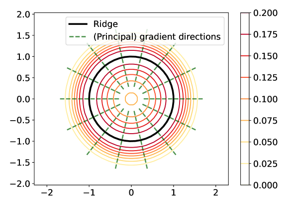
Figure 2: Contour lines of the density function (24) and its principal gradient flows.

Condition (A4) imposes a direct assumption on the SCGA sequence $\big{\{}\bm{x}^{(t)}\big{\}}_{t=0}^{\infty}$, under which the residual vector $U_{d}^{\perp}(\bm{x}^{(t)})(\bm{x}^{*}-\bm{x}^{(t)})$ and its inner product with the residual gradient $U^{\perp}(\bm{x}^{(t)})\nabla p(\bm{x}^{(t)})$ are upper bounded by a quadratic term $O\left(\left|\left|\bm{x}^{*}-\bm{x}^{(t)}\right|\right|_{2}^{2}\right)$. This condition is imposed to guarantee that $p$ is “subspace constrained strongly concave” around $R_{d}$; see also Remark 3.3. Our proof of Theorem 3.6 suggests that the residual vector $U_{d}^{\perp}(\bm{x}^{(t)})(\bm{x}^{*}-\bm{x}^{(t)})$ is only required to be smaller than the first-order term $o\left(\left|\left|\bm{x}^{(t)}-\bm{x}^{*}\right|\right|_{2}\right)$. For the simplicity, we require it to be quadratic. When condition (A4) fails to hold, the associated SCGA sequence can only converge sublinearly to $R_{d}$. Therefore, it is an essential element in the linear convergence of the SCGA algorithm, and we discuss some potentially weaker assumptions that implicate condition (A4) in Appendix E. Intuitively, the SCGA path converges to $R_{d}$ following the direction of principal gradient $V_{d}(\bm{x}^{(t)})V_{d}(\bm{x}^{(t)})^{T}\nabla p(\bm{x}^{(t)})$. To further gain more insights into the correctness of condition (A4), we consider a special density function

$$p(u,v)=C_{p,2}\cdot\exp\left[-\left(u^{2}+v^{2}-1\right)^{2}\right]\quad\text{ with }\quad C_{p,2}=\pi\left(\frac{\sqrt{\pi}}{2}+\int_{0}^{1}e^{-t^{2}}dt\right)$$ (24)

on $\mathbb{R}^{2}$, whose one-dimensional ridge is $R_{1}=\left\{(u,v)\in\mathbb{R}^{2}:u^{2}+v^{2}=1\right\}$ by the definition (1). Some careful calculations suggest that its principal gradient $G_{1}(u,v)$ points towards the ridge $R_{1}$ in the direction $(u,v)$ when $\frac{2-\sqrt{2}}{2}<u^{2}+v^{2}<1$ and in the direction $(-u,-v)$ when $1<u^{2}+v^{2}<\frac{2+\sqrt{2}}{2}$; see Figure 2 for a graphical illustration. Furthermore, the smallest eigenvalue of $\nabla\nabla p(u,v)$ is negative whenever $u^{2}+v^{2}>\frac{1}{2}$. Hence, the residual gradient $U_{1}^{\perp}(u,v)\nabla p(u,v)$ is perpendicular to the SCGA direction, and condition (A4) naturally holds.

We now present our linear convergence results for the population and sample-based SCGA algorithms.

Theorem 3.6 (Linear Convergence of the SCGA Algorithm).

Assume conditions (A1-4) throughout the theorem.

1. Q-Linear convergence of $\left|\left|\bm{x}^{(t)}-\bm{x}^{*}\right|\right|_{2}$: Consider a convergence radius $r_{2}>0$ satisfying

   $$0<r_{2}<\min\left\{\frac{\rho}{2},\frac{\beta_{1}^{2}}{A_{2}\left(\left|\left|p\right|\right|_{\infty}^{(3)}+\left|\left|p\right|\right|_{\infty}^{(4)}\right)},\frac{\beta_{1}}{A_{4}(p)},\frac{3\beta_{0}}{4D\left(6\left|\left|p\right|\right|_{\infty}^{(2)}\beta_{2}^{2}\rho+D^{\frac{1}{2}}\left|\left|p\right|\right|_{\infty}^{(3)}\right)}\right\},$$

   where $A_{2}>0$ is the constant defined in (h) of Lemma C.1 and $A_{4}(p)>0$ is a quantity defined in (c) of Proposition 3.3 that depends on both the dimension $D$ and the functional norm $\left|\left|p\right|\right|_{\infty,4}^{*}$ up to the fourth-order derivative of $p$. Whenever $0<\eta\leq\min\left\{\frac{4}{\beta_{0}},\frac{1}{D\left|\left|p\right|\right|_{\infty}^{(2)}}\right\}$ and the initial point $\bm{x}^{(0)}\in\text{Ball}_{D}(\bm{x}^{*},r_{2})$ with $\bm{x}^{*}\in R_{d}$, we have that

   $$\left|\left|\bm{x}^{(t)}-\bm{x}^{*}\right|\right|_{2}\leq\Upsilon^{t}\left|\left|\bm{x}^{(0)}-\bm{x}^{*}\right|\right|_{2}\quad\text{ with }\quad\Upsilon=\sqrt{1-\frac{\beta_{0}\eta}{4}}.$$

2. R-Linear convergence of $d_{E}(\bm{x}^{(t)},R_{d})$: Under the same radius $r_{2}>0$ in (a), we have that whenever $0<\eta\leq\min\left\{\frac{4}{\beta_{0}},\frac{1}{D\left|\left|p\right|\right|_{\infty}^{(2)}}\right\}$ and the initial point $\bm{x}^{(0)}\in\text{Ball}_{D}(\bm{x}^{*},r_{2})$ with $\bm{x}^{*}\in R_{d}$,

   $$d_{E}(\bm{x}^{(t)},R_{d})\leq\Upsilon^{t}\left|\left|\bm{x}^{(0)}-\bm{x}^{*}\right|\right|_{2}\quad\text{ with }\quad\Upsilon=\sqrt{1-\frac{\beta_{0}\eta}{4}}.$$

We further assume conditions (E1-2) in the rest of statements. If $h\to 0$ and $\frac{nh^{D+4}}{|\log h|}\to\infty$,

1. Q-Linear convergence of $\left|\left|\widehat{\bm{x}}^{(t)}-\bm{x}^{*}\right|\right|_{2}$: under the same radius $r_{2}>0$ and $\Upsilon=\sqrt{1-\frac{\beta_{0}\eta}{4}}$ in (a), we have that

   $$\left|\left|\widehat{\bm{x}}^{(t)}-\bm{x}^{*}\right|\right|_{2}\leq\Upsilon^{t}\left|\left|\widehat{\bm{x}}^{(0)}-\bm{x}^{*}\right|\right|_{2}+O(h^{2})+O_{P}\left(\sqrt{\frac{|\log h|}{nh^{D+4}}}\right)$$

   with probability tending to 1 whenever $0<\eta\leq\min\left\{\frac{4}{\beta_{0}},\frac{1}{D\left|\left|p\right|\right|_{\infty}^{(2)}}\right\}$ and the initial point $\widehat{\bm{x}}^{(0)}\in\text{Ball}_{D}(\bm{x}^{*},r_{2})$ with $\bm{x}^{*}\in R_{d}$.

1. R-Linear convergence of $d_{E}(\widehat{\bm{x}}^{(t)},R_{d})$: under the same radius $r_{2}>0$ and $\Upsilon=\sqrt{1-\frac{\beta_{0}\eta}{4}}$ in (a), we have that

   $$d_{E}(\widehat{\bm{x}}^{(t)},R_{d})\leq\Upsilon^{t}\left|\left|\widehat{\bm{x}}^{(0)}-\bm{x}^{*}\right|\right|_{2}+O(h^{2})+O_{P}\left(\sqrt{\frac{|\log h|}{nh^{D+4}}}\right)$$

   with probability tending to 1 whenever $0<\eta\leq\min\left\{\frac{4}{\beta_{0}},\frac{1}{D\left|\left|p\right|\right|_{\infty}^{(2)}}\right\}$ and the initial point $\widehat{\bm{x}}^{(0)}\in\text{Ball}_{D}(\bm{x}^{*},r_{2})$ with $\bm{x}^{*}\in R_{d}$.

The detailed proof of Theorem 3.6 can be found in Appendix D. Note that, as in (c) of Proposition 3.3, we elucidate a threshold value for the convergence radius $r_{2}>0$ in (a), under which the population SCGA algorithm converges linearly to $R_{d}$. The first three quantities in the threshold value are directly adopted from the upper bound of the convergence radius $r_{1}$ in (c) of Proposition 3.3, while the last term controls the “subspace constrained strongly concavity” (26) of $p$ within $R_{d}\oplus r_{2}$.

Remark 3.3.

Notice that the standard strong concavity assumption on the objective function (or density function) $p$ is not sufficient to establish the linear convergence of the population SCGA algorithm (23). This is because, under the (quasi-)strong concavity assumption (Necoara et al., 2019), the objective function $p$ would satisfy

$$p(\bm{x}^{*})-p(\bm{y})\leq\nabla p(\bm{y})^{T}(\bm{x}^{*}-\bm{y})-\frac{A_{6}}{2}\left|\left|\bm{x}^{*}-\bm{y}\right|\right|_{2}^{2}$$ (25)

for some constant $A_{6}>0$, and those standard proofs of the linear convergence of gradient ascent methods rely on this inequality; see Section 3.4 in Bubeck (2015). However, as indicated in our proof of Theorem 3.6, the linear convergence of the SCGA algorithm requires the following inequality instead:

$$p(\bm{x}^{*})-p(\bm{y})\leq\nabla p(\bm{y})^{T}V_{d}(\bm{y})V_{d}(\bm{y})^{T}(\bm{x}^{*}-\bm{y})-\frac{A_{7}}{2}\left|\left|\bm{x}^{*}-\bm{y}\right|\right|_{2}^{2}+o\left(\left|\left|\bm{x}^{*}-\bm{y}\right|\right|_{2}^{2}\right)$$ (26)

for some constant $A_{7}>0$, where $\bm{y}$ is generally chosen to be $\bm{x}^{(t)}$. We call the function $p$ satisfying (26) to be “subspace constrained strongly concave”. Since

$$\nabla p(\bm{y})^{T}(\bm{x}^{*}-\bm{y})=\nabla p(\bm{y})^{T}V_{d}(\bm{y})V_{d}(\bm{y})^{T}(\bm{x}^{*}-\bm{y})+\nabla p(\bm{y})^{T}U_{d}^{\perp}(\bm{y})(\bm{x}^{*}-\bm{y}),$$

the strong concavity assumption (25) will not imply the key inequality (26) for the linear convergence of the population SCGA algorithm unless the residual gradient term $\nabla p(\bm{y})^{T}U_{d}^{\perp}(\bm{y})(\bm{x}^{*}-\bm{y})$ can be upper bounded by the second-order error term $O\left(\left|\left|\bm{x}^{*}-\bm{y}\right|\right|_{2}^{2}\right)$. The imposed eigengap condition (A2) as well as condition (A4) with its related discussion in Appendix E fill in this gap, ensuring that such a quadratic upper bound holds on the residual gradients along the SCGA sequence.

Corollary 3.7 (Linear Convergence of the SCMS Algorithm).

Assume conditions (A1-4) and (E1-2). When the fixed sample size $n$ is sufficiently large and the bandwidth $h$ is chosen to be sufficiently small, there exists a convergence radius $r_{3}\in(0,r_{2})$ such that the SCMS sequence $\big{\{}\widehat{\bm{x}}^{(t)}\big{\}}_{t=0}^{\infty}$ satisfies the following property with high probability:

$$d_{E}(\widehat{\bm{x}}^{(t)},\widehat{R}_{d})\leq\left|\left|\widehat{\bm{x}}^{(t)}-\widehat{\bm{x}}^{*}\right|\right|_{2}\leq\Upsilon_{n,h}^{t}\left|\left|\widehat{\bm{x}}^{(0)}-\widehat{\bm{x}}^{*}\right|\right|_{2}$$

$$\text{ with }\quad\Upsilon_{n,h}=\sqrt{1-\frac{\beta_{0}\widetilde{\eta}_{n,h}}{4}}\quad\text{ and }\quad\widetilde{\eta}_{n,h}=\inf_{t}\eta_{n,h}^{(t)}$$

whenever $0<\sup_{t}\eta_{n,h}^{(t)}\leq\min\left\{\frac{4}{\beta_{0}},\frac{1}{D\left|\left|p\right|\right|_{\infty}^{(2)}}\right\}$ and the initial point $\widehat{\bm{x}}^{(0)}\in\widehat{R}_{d}\oplus r_{3}$.

Corollary 3.7 should also be regarded as the linear convergence of the sample-based SCGA algorithm to the estimated ridge $\widehat{R}_{d}$ defined by the Euclidean KDE $\widehat{p}_{n}$. Based on conditions (E1-2) and the uniform bounds (16), $\widehat{p}_{n}$ together with its ridge $\widehat{R}_{d}$ and sample-based SCGA sequence $\big{\{}\widehat{\bm{x}}^{(t)}\big{\}}_{t=0}^{\infty}$ satisfy conditions (A1-4) with probability tending to 1 as $h\to 0$ and $\frac{nh^{D+6}}{|\log h|}\to\infty$. As a result, one can follow our argument in (a) of Theorem 3.6 to establish the linear convergence of the sample-based SCGA algorithm with a fixed step size $\eta$ satisfying $0<\eta\leq\min\left\{\frac{4}{\beta_{0}},\frac{1}{D\left|\left|p\right|\right|_{\infty}^{(2)}}\right\}$. Furthermore, when the fixed sample size $n$ is sufficiently large and the bandwidth $h$ is chosen to be small, the adaptive step size $\eta_{n,h}^{(t)}$ of the SCMS algorithm always falls below the threshold $\min\left\{\frac{4}{\beta_{0}},\frac{1}{D\left|\left|p\right|\right|_{\infty}^{(2)}}\right\}$ for linear convergence but is also uniformly bounded away from zero with respect to the iteration number $t$; see our Remark 3.2. By taking the infimum of the adaptive step size $\eta_{n,h}^{(t)}$ with respect to $t$, one can thus establish the linear convergence of the SCMS algorithm with its rate of convergence as $\Upsilon_{n,h}=\sqrt{1-\frac{\beta_{0}\widetilde{\eta}_{n,h}}{4}}$ and $\widetilde{\eta}_{n,h}=\inf_{t}\eta_{n,h}^{(t)}$.

4 The SCMS Algorithm With Directional Data and Its Linear Convergence

In this section, we generalize the definition (1) of density ridges to directional densities on $\Omega_{q}$ and propose our directional SCMS algorithm to identify directional density ridges. In addition, we prove the linear convergence of our directional SCMS algorithm by adjusting the arguments in Section 3.3. Throughout this section, $\left\{\bm{X}_{1},...,\bm{X}_{n}\right\}$ denotes a random sample from a directional distribution with density $f$ supported on the unit hypersphere $\Omega_{q}$ that is embedded in the ambient Euclidean space $\mathbb{R}^{q+1}$.

4.1 Definitions, Assumptions, and Stability of Directional Density Ridges

To apply the matrix forms of the Riemannian gradient $\mathtt{grad}\,f(\bm{x})$ and Hessian $\mathcal{H}f(\bm{x})$ of a directional density $f$ in the ambient space $\mathbb{R}^{q+1}$, we first extend $f$ from its support $\Omega_{q}$ to $\mathbb{R}^{q+1}\setminus\left\{\bm{0}\right\}$ by defining

$$f(\bm{x})\equiv f\left(\frac{\bm{x}}{||\bm{x}||_{2}}\right)\quad\text{ for all }\quad\bm{x}\in\mathbb{R}^{q+1}\setminus\{\bm{0}\}.$$ (27)

Now, given the expressions of $\mathtt{grad}\,f(\bm{x})$ and $\mathcal{H}f(\bm{x})$ defined in (9) and (11), we perform the spectral decomposition on $\mathcal{H}f(\bm{x})$ as $\mathcal{H}f(\bm{x})=\underline{V}(\bm{x})\underline{\Lambda}(\bm{x})\underline{V}(\bm{x})^{T}$, where $\underline{V}(\bm{x})=\left[\bm{x},\underline{\bm{v}}_{1}(\bm{x}),...,\underline{\bm{v}}_{q}(\bm{x})\right]\in\mathbb{R}^{(q+1)\times(q+1)}$ is a real orthogonal matrix with columns $\underline{\bm{v}}_{1}(\bm{x}),...,\underline{\bm{v}}_{q}(\bm{x})$ as the eigenvectors of $\mathcal{H}f(\bm{x})$ that are associated with the eigenvalues $\underline{\lambda}_{1}(\bm{x})\geq\cdots\geq\underline{\lambda}_{q}(\bm{x})$ and lie within the tangent space $T_{\bm{x}}$ at $\bm{x}\in\Omega_{q}$, and $\underline{\Lambda}(\bm{x})=\mathtt{Diag}\left[0,\underline{\lambda}_{1}(\bm{x}),...,\underline{\lambda}_{q}(\bm{x})\right]$. Note that the Riemannian Hessian $\mathcal{H}f(\bm{x})$ has a unit eigenvector $\bm{x}$ that is orthogonal to $T_{\bm{x}}$ and corresponds to eigenvalue 0.

Let $\underline{V}_{d}(\bm{x})=\left[\underline{\bm{v}}_{d+1}(\bm{x}),...,\underline{\bm{v}}_{q}(\bm{x})\right]\in\mathbb{R}^{(q+1)\times(q-d)}$ be the last $q-d$ columns of $\underline{V}(\bm{x})$, i.e., the unit eigenvectors inside the tangent space $T_{\bm{x}}$ corresponding to the $q-d$ smallest eigenvalues of $\mathcal{H}f(\bm{x})$. Let $\underline{U}_{d}(\bm{x})=\underline{V}_{d}(\bm{x})\underline{V}_{d}(\bm{x})^{T}$ be the projection matrix onto the linear space spanned by the columns of $\underline{V}_{d}(\bm{x})$, and $\underline{U}_{d}^{\perp}(\bm{x})=\bm{I}_{q+1}-\underline{V}_{d}(\bm{x})\underline{V}_{d}(\bm{x})^{T}$. We define the order-$d$ principal Riemannian gradient $\underline{G}_{d}(\bm{x})$ by:

$$\begin{split}\underline{G}_{d}(\bm{x})=\underline{V}_{d}(\bm{x})\underline{V}_{d}(\bm{x})^{T}\mathtt{grad}\,f(\bm{x})&=\underline{V}_{d}(\bm{x})\underline{V}_{d}(\bm{x})^{T}\left(\bm{I}_{q+1}-\bm{x}\bm{x}^{T}\right)\nabla f(\bm{x})\\ &=\underline{V}_{d}(\bm{x})\underline{V}_{d}(\bm{x})^{T}\nabla f(\bm{x}),\end{split}$$ (28)

where the last equality follows from the fact that the columns of $\underline{V}_{d}(\bm{x})$ are orthogonal to the unit vector $\bm{x}$. The order-$d$ density ridge on $\Omega_{q}$ (or directional density ridge) is the set of points defined as:

$$\begin{split}\underline{R}_{d}&=\left\{\bm{x}\in\Omega_{q}:\underline{G}_{d}(\bm{x})=\bm{0},\underline{\lambda}_{d+1}(\bm{x})<0\right\}\\ &=\left\{\bm{x}\in\Omega_{q}:\underline{V}_{d}(\bm{x})^{T}\mathtt{grad}\,f(\bm{x})=\bm{0},\underline{\lambda}_{d+1}(\bm{x})<0\right\}.\end{split}$$ (29)

Our definition of density ridges on $\Omega_{q}$ can be arguably generalized to any smooth function $f$ supported on an arbitrary Riemannian manifold. It also follows that the 0-ridge $\underline{R}_{0}$ is the set of local modes of $f$ on $\Omega_{q}$, whose statistical properties and practical estimation algorithm are discussed in Zhang and Chen (2021a). Therefore, we only focus on the case when $1\leq d<q$ in this paper. To regularize the directional density ridge $\underline{R}_{d}$, we modify our assumptions on the Euclidean density ridge $R_{d}$ in Section 3.1 as follows:

• (A1) (Differentiability) Under the extension (27) of the directional density $f$, we assume that the total gradient $\nabla f(\bm{x})$, total Hessian matrix $\nabla\nabla f(\bm{x})$, and third-order derivative tensor $\nabla^{3}f(\bm{x})$ in $\mathbb{R}^{q+1}$ exist, and are continuous on $\mathbb{R}^{q+1}\setminus\{\bm{0}\}$ and square integrable on $\Omega_{q}$. We also assume that $f$ has bounded fourth order derivatives on $\Omega_{q}$.

• (A2) (Eigengap) We assume that there exist constants $\underline{\rho}>0$ and $\underline{\beta}_{0}>0$ such that $\underline{\lambda}_{d+1}(\bm{y})\leq-\underline{\beta}_{0}$ and $\underline{\lambda}_{d}(\bm{y})-\underline{\lambda}_{d+1}(\bm{y})\geq\underline{\beta}_{0}$ for any $\bm{y}\in\left(\underline{R}_{d}\oplus\underline{\rho}\right)\cap\Omega_{q}$.

• (A3) (Path Smoothness) Under the same $\underline{\rho},\underline{\beta}_{0}>0$ in (A2), we assume that there exists another constant $\underline{\beta}_{1}\in\left(0,\underline{\beta}_{0}\right)$ such that

  $$\sqrt{2}\cdot q^{\frac{3}{2}}\left|\left|\underline{U}_{d}^{\perp}(\bm{y})\mathtt{grad}\,f(\bm{y})\right|\right|_{2}\left|\left|\nabla^{3}f(\bm{y})\right|\right|_{\max} \leq\frac{\underline{\beta}_{0}^{2}}{2},$$

  $$d\cdot q^{\frac{3}{2}}\left|\left|\nabla f(\bm{x})\right|\right|_{2}\cdot\left|\left|\nabla^{3}f(\bm{x})\right|\right|_{\max} \leq\underline{\beta}_{0}\left(\underline{\beta}_{0}-\underline{\beta}_{1}\right)$$

  for all $\bm{y}\in\left(\underline{R}_{d}\oplus\underline{\rho}\right)\cap\Omega_{q}$ and $\bm{x}\in\underline{R}_{d}$.

Recall that $\underline{R}_{d}\oplus\underline{\rho}=\cup_{\bm{x}\in\underline{R}_{d}}\text{Ball}_{q+1}\big{(}\bm{x},\underline{\rho}\big{)}$ is a $\underline{\rho}$-neighborhood of the directional ridge $\underline{R}_{d}$ in the ambient space $\mathbb{R}^{q+1}$. The discussions about conditions (A1-3) in Section 3.1 apply to their directional counterparts (A1-3), except that the eigengap condition (A2) is imposed on eigenvalues $\underline{\lambda}_{1}(\bm{x})\geq\cdots\geq\underline{\lambda}_{q}(\bm{x})$ within the tangent space $T_{\bm{x}}$ at $\bm{x}\in\Omega_{q}$. However, since the only eigenvalue of $\mathcal{H}f(\bm{x})$ associated with the eigenvector outside the tangent space $T_{\bm{x}}$ is 0, the eigengap condition (A2) is also valid to the entire spectrum of $\mathcal{H}f(\bm{x})$ in the ambient space $\mathbb{R}^{q+1}$. The extension of $f$ in (27) has also been used by Zhao and Wu (2001); García-Portugués et al. (2013); García-Portugués (2013). Because the directional density $f$ remains unchanged along every radial direction of $\Omega_{q}$ under the extension (27), the radial component of its total gradient is $\mathtt{Rad}\left(\nabla f(\bm{x})\right)=0$ for all $\bm{x}\in\Omega_{q}$, and the Riemannian gradient (9) of $f$ on $\Omega_{q}$ becomes

$$\mathtt{grad}\,(\bm{x})=\left(\bm{I}_{q+1}-\bm{x}\bm{x}^{T}\right)\nabla f(\bm{x})=\nabla f(\bm{x}).$$ (30)

Similarly, the Riemannian Hessian (11) of $f$ on $\Omega_{q}$ reduces to

$$\mathcal{H}f(\bm{x})=\left(\bm{I}_{q+1}-\bm{x}\bm{x}^{T}\right)\nabla\nabla f(\bm{x})\left(\bm{I}_{q+1}-\bm{x}\bm{x}^{T}\right).$$ (31)

Both the Riemannian gradient and Hessian of $f$ on $\Omega_{q}$ are invariant under this extension.

Remark 4.1 (Connection to Solution Manifolds).

Example 4 in Chen (2020) showed that any Euclidean density ridge $R_{d}$ defined in (1) is a concrete example of a solution manifold $\mathcal{M}_{S}=\left\{\bm{x}\in\mathbb{R}^{D}:\Psi(\bm{x})=0\right\}$ with $\Psi:\mathbb{R}^{D}\to\mathbb{R}^{D-d}$ being a vector-valued function. It is not difficult to verify that our defined directional density ridge $\underline{R}_{d}$ in (29) also belongs to the general form of the solution manifold $\mathcal{M}_{S}$, where we may rewrite $\underline{R}_{d}=\left\{\bm{x}\in\mathbb{R}^{q+1}:\Psi(\bm{x})=0\right\}$ with $\Psi:\mathbb{R}^{q+1}\to\mathbb{R}^{q+1-d}$ defined by:

$$\Psi(\bm{x})=\begin{bmatrix}\underline{\bm{v}}_{d+1}(\bm{x})^{T}\nabla f(\bm{x})\\ \vdots\\ \underline{\bm{v}}_{q}(\bm{x})^{T}\nabla f(\bm{x})\\ \bm{x}^{T}\bm{x}-1\end{bmatrix},$$

recalling that $\underline{\bm{v}}_{d+1}(\bm{x}),...,\underline{\bm{v}}_{q}(\bm{x})$ are the last $q-d$ eigenvectors of the Riemannian Hessian $\mathcal{H}f(\bm{x})$ of the directional density $f$. More importantly, our imposed conditions (A1-3) in the Euclidean ridge case and (A1-3) in the directional ridge case imply all the required assumptions in Chen (2020), i.e., the differentiability of $\Psi$ and non-degeneracy of the normal space of $\mathcal{M}_{S}$; see (d) of Lemmas C.1 and G.1 in the Appendix. Therefore, the discussion about statistical properties and (normal) gradient flows of a generic solution manifold $\mathcal{M}_{S}$ apply to the (directional) density ridge $R_{d}$ or $\underline{R}_{d}$ here.

Similar to Euclidean density ridges, we establish the following stability theorem of directional density ridges. To measure the distance between two directional ridges $\underline{R}_{d},\underline{\widetilde{R}}_{d}\subset\Omega_{q}$ defined by the directional densities $f$ and $\widetilde{f}$, we adopt the definition (15) of Hausdorff distance between two sets in the ambient Euclidean space $\mathbb{R}^{q+1}$. Note that the Euclidean norm used in the definition (15) is upper bounded by the geodesic distance when our interested sets lie on $\Omega_{q}$; see also (6). We will leverage this property in our proof of Theorem 4.1; see Appendix H for details.

Theorem 4.1.

Suppose that conditions (A1-3) hold for the directional density $f$ and that condition (A1) holds for $\widetilde{f}$. When $\left|\left|f-\widetilde{f}\right|\right|_{\infty,3}^{*}$ is sufficiently small,

1. conditions (A2-3) holds for $\widetilde{f}$.

2. $\mathtt{Haus}(\underline{R}_{d},\underline{\widetilde{R}}_{d})=O\left(\left|\left|f-\widetilde{f}\right|\right|_{\infty,2}^{*}\right)$.

3. $\mathtt{reach}(\underline{\widetilde{R}}_{d})\geq\min\left\{\underline{\rho}/2,\frac{\min\left\{\underline{\beta}_{1},1\right\}^{2}}{\underline{A}_{2}\left(\left|\left|f\right|\right|_{\infty}^{(3)}+\left|\left|f\right|\right|_{\infty}^{(4)}\right)}\right\}+O\left(\left|\left|f-\widetilde{f}\right|\right|_{\infty,3}^{*}\right)$ for a constant $\underline{A}_{2}>0$.

One natural estimator of the directional density ridge $\underline{R}_{d}$ can be obtained by plugging the directional KDE $\widehat{f}_{h}$ into the definition (29) as:

$$\widehat{\underline{R}}_{d}=\left\{\bm{x}\in\Omega_{q}:\widehat{\underline{V}}_{d}(\bm{x})^{T}\mathtt{grad}\,\widehat{f}_{h}(\bm{x})=\bm{0},\widehat{\underline{\lambda}}_{d+1}(\bm{x})<0\right\}.$$

To regularize the statistical behavior of the estimated directional ridge $\widehat{\underline{R}}_{d}$, we consider the following assumptions that are generalized from conditions (E1-2):

• (D1) Assume that $L:(-\delta_{L},\infty)\to[0,\infty)$ is a bounded and three times continuously differentiable function with a bounded fourth order derivative on $(-\delta_{L},\infty)\subset\mathbb{R}$ for some constant $\delta_{L}>0$ such that

  $$0<\int_{0}^{\infty}|L^{(\ell)}(r)|^{k}r^{\frac{q}{2}-1}dr<\infty\quad\text{ for all }q\geq 1,k=1,2,\text{ and }\ell=0,1,2,3.$$

• (D2) Let

  $$\mathcal{K}_{D}=\left\{\bm{u}\mapsto K\left(\frac{\bm{z}-\bm{u}}{h}\right):\bm{u},\bm{z}\in\Omega_{q},h>0,K(\bm{x})=D^{[\tau]}L\left(\frac{\left|\left|\bm{x}\right|\right|_{2}^{2}}{2}\right),|[\tau]|=0,1,2,3\right\}.$$

  We assume that $\mathcal{K}_{D}$ is a bounded VC (subgraph) class of measurable functions on $\Omega_{q}$; that is, there exist constants $A,\upsilon>0$ such that for any $0<\epsilon<1$,

  $$\sup_{Q}N\left(\mathcal{K}_{D},L_{2}(Q),\epsilon||F||_{L_{2}(Q)}\right)\leq\left(\frac{A}{\epsilon}\right)^{\upsilon},$$

  where $N(\mathcal{K}_{D},L_{2}(Q),\epsilon)$ is the $\epsilon$-covering number of the normed space $\left(\mathcal{K}_{D},\left|\left|\cdot\right|\right|_{L_{2}(Q)}\right)$, $Q$ is any probability measure on $\Omega_{q}$, and $F$ is an envelope function of $\mathcal{K}_{D}$. Here, the norm $\left|\left|F\right|\right|_{L_{2}(Q)}$ is defined as $\left[\int_{\Omega_{q}}|F(\bm{x})|^{2}dQ(\bm{x})\right]^{\frac{1}{2}}$.

The differentiability assumption in condition (D1) can be relaxed such that $L$ is (three times) continuously differentiable except for a set of points with Lebesgue measure $0$ on $[0,\infty)$. Conditions (D1) and (A1) are generally required for establishing the pointwise convergence rates of the directional KDE and its derivatives (Hall et al., 1987; Klemelä, 2000; Zhao and Wu, 2001; García-Portugués et al., 2013; García-Portugués, 2013). Under these two conditions, $\left|\left|\nabla\widehat{f}_{h}(\bm{x})\right|\right|_{2}$ appearing in the step sizes $\underline{\eta}_{n,h}^{(t)}$ or $\underline{\eta}_{n,h}^{(t)^{\prime}}$ of the directional mean shift or SCMS algorithm can also be shown to diverge at the order $O(h^{-2})+O_{P}\left(\frac{1}{nh^{q+2}}\right)$ as $nh^{q}\to\infty$ and $h\to 0$; see Section 4.2 for details. Condition (D2) regularizes the complexity of kernel $L$ and its derivatives as in condition (E2) in order for the uniform convergence rates of the directional KDE and its derivatives; see (32) below. One can justify via integration by parts that the von-Mises kernel $L(r)=e^{-r}$ and many compactly supported kernels satisfy conditions (D1-2).

Given conditions (D1-2), the techniques in Hall et al. (1987); Bai et al. (1988); Zhao and Wu (2001); García-Portugués et al. (2013); García-Portugués (2013); Zhang and Chen (2021a) can be utilized to demonstrate that

$$\left|\left|\widehat{f}_{h}-f\right|\right|_{\infty}^{(k)}=\sup_{\bm{x}\in\Omega_{q}}\left|\left|\bar{\nabla}^{k}\,\widehat{f}_{h}(\bm{x})-\bar{\nabla}^{k}\,f(\bm{x})\right|\right|_{\max}=O(h^{2})+O_{P}\left(\sqrt{\frac{|\log h|}{nh^{q+2k}}}\right),$$ (32)

where $\bar{\nabla}\equiv\bar{\nabla}_{\bm{v}}$ is the Riemannian connection on $\Omega_{q}$ with $\bm{v}\in T_{\bm{x}}$ so that $\bar{\nabla}f(\bm{x})=\mathtt{grad}\,f(\bm{x})$, $\bar{\nabla}^{2}f(\bm{x})=\mathcal{H}f(\bm{x})$, and $\bar{\nabla}^{3}f(\bm{x})=\bar{\nabla}\mathcal{H}f(\bm{x})$; see Section 5.3 in Absil et al. (2008) and Chapter 4 in Lee (2018).

4.2 Mean Shift and SCMS Algorithm with Directional Data

Before deriving our directional SCMS algorithm, we first review the mean shift algorithm with directional data $\left\{\bm{X}_{1},...,\bm{X}_{n}\right\}\subset\Omega_{q}$ (Oba et al., 2005; Kafai et al., 2010; Yang et al., 2014). The formal derivation can be found in Section 3 of Zhang and Chen (2021a). Given the directional KDE $\widehat{f}_{h}(\bm{x})=\frac{c_{L,q}(h)}{n}\sum\limits_{i=1}^{n}L\left(\frac{1-\bm{x}^{T}\bm{X}_{i}}{h^{2}}\right)$ in (5), the directional mean shift vector can be defined as:

$$\underline{\Xi}_{h}(\bm{x})=\frac{\sum_{i=1}^{n}\bm{X}_{i}L^{\prime}\left(\frac{1}{2}\left|\left|\frac{\bm{x}-\bm{X}_{i}}{h}\right|\right|_{2}^{2}\right)}{\sum_{i=1}^{n}L^{\prime}\left(\frac{1}{2}\left|\left|\frac{\bm{x}-\bm{X}_{i}}{h}\right|\right|_{2}^{2}\right)}-\bm{x}=\frac{\sum_{i=1}^{n}\bm{X}_{i}L^{\prime}\left(\frac{1-\bm{x}^{T}\bm{X}_{i}}{h^{2}}\right)}{\sum_{i=1}^{n}L^{\prime}\left(\frac{1-\bm{x}^{T}\bm{X}_{i}}{h^{2}}\right)}-\bm{x}.$$ (33)

Similar to the Euclidean mean shift vector (18), $\underline{\Xi}_{h}(\bm{x})$ also points toward the direction of maximum increase in $\widehat{f}_{h}(\bm{x})$ after being projected onto the tangent space $T_{\bm{x}}$. Thus, the directional mean shift iteration translates a point $\bm{x}\in\Omega_{q}$ as $\bm{x}+\underline{\Xi}_{h}(\bm{x})$ with an extra projection $\frac{\bm{x}+\underline{\Xi}_{h}(\bm{x})}{\left|\left|\bm{x}+\underline{\Xi}_{h}(\bm{x})\right|\right|_{2}}$ to draw the shifted point back to $\Omega_{q}$.

Let $\{\underline{\widehat{\bm{x}}}^{(t)}\}_{t=0}^{\infty}$ denote the sequence defined by the above directional mean shift procedure. Later, by abuse of notation, we will use the same notation to denote the directional SCGA/SCMS sequence with $\widehat{f}_{h}$. As $\nabla\widehat{f}_{h}(\bm{x})=-\frac{c_{L,q}(h)}{nh^{2}}\sum\limits_{i=1}^{n}\bm{X}_{i}L^{\prime}\left(\frac{1-\bm{x}^{T}\bm{X}_{i}}{h^{2}}\right)$, some simple algebra shows that the directional mean shift algorithm can be written into the following fixed-point iteration formula:

$$\underline{\widehat{\bm{x}}}^{(t+1)}=-\frac{\sum_{i=1}^{n}\bm{X}_{i}L^{\prime}\left(\frac{1-\bm{X}_{i}^{T}\underline{\widehat{\bm{x}}}^{(t)}}{h^{2}}\right)}{\left|\left|\sum_{i=1}^{n}\bm{X}_{i}L^{\prime}\left(\frac{1-\bm{X}_{i}^{T}\underline{\widehat{\bm{x}}}^{(t)}}{h^{2}}\right)\right|\right|_{2}}\quad\text{ or }\quad\underline{\widehat{\bm{x}}}^{(t+1)}=\frac{\nabla\widehat{f}_{h}\left(\underline{\widehat{\bm{x}}}^{(t)}\right)}{\left|\left|\nabla\widehat{f}_{h}\left(\underline{\widehat{\bm{x}}}^{(t)}\right)\right|\right|_{2}}.$$ (34)

From (34), it is also possible to write the directional mean shift algorithm as a gradient ascent method on $\Omega_{q}$ with the iteration formula (Zhang and Sra, 2016):

$$\widehat{\underline{\bm{x}}}^{(t+1)}=\mathtt{Exp}_{\widehat{\underline{\bm{x}}}^{(t)}}\left(\underline{\eta}_{n,h}^{(t)}\cdot\mathtt{grad}\,\widehat{f}_{h}(\widehat{\underline{\bm{x}}}^{(t)})\right),$$ (35)

where the adaptive step size $\underline{\eta}_{n,h}^{(t)}$ is given by

$$\underline{\eta}_{n,h}^{(t)}=\arccos\left(\frac{\nabla\widehat{f}_{h}\left(\underline{\widehat{\bm{x}}}^{(t)}\right)^{T}\underline{\widehat{\bm{x}}}^{(t)}}{\left|\left|\nabla\widehat{f}_{h}\left(\underline{\widehat{\bm{x}}}^{(t)}\right)\right|\right|_{2}}\right)\cdot\frac{1}{\left|\left|\mathtt{grad}\,\widehat{f}_{h}(\underline{\widehat{\bm{x}}}^{(t)})\right|\right|_{2}}=\frac{\theta_{t}}{\left|\left|\nabla\widehat{f}_{h}(\underline{\widehat{\bm{x}}}^{(t)})\right|\right|_{2}\cdot\sin\theta_{t}}.$$ (36)

Here, we denote the angle between $\underline{\widehat{\bm{x}}}^{(t+1)}$ and $\underline{\widehat{\bm{x}}}^{(t)}$ (or equivalently, the angle between $\nabla\widehat{f}_{h}(\underline{\widehat{\bm{x}}}^{(t)})$ and $\underline{\widehat{\bm{x}}}^{(t)}$) by $\theta_{t}$; see Section 5.2 in Zhang and Chen (2021a) for detailed derivations. Within some small neighborhoods around local modes of $\widehat{f}_{h}$, $\frac{\theta_{t}}{\sin\theta_{t}}\approx 1$ and the adaptive step size $\underline{\eta}_{n,h}^{(t)}$ will be dominated by $\left|\left|\nabla\widehat{f}_{h}(\underline{\widehat{\bm{x}}}^{(t)})\right|\right|_{2}$. The following lemma characterizes the asymptotic behaviors of $\left|\left|\nabla\widehat{f}_{h}(\bm{x})\right|\right|_{2}$ on $\Omega_{q}$ and consequently, $\underline{\eta}_{n,h}^{(t)}$.

Lemma 4.2 (Lemma 10 in Zhang and Chen 2021a).

Assume conditions (D1) and (A1). For any fixed $\bm{x}\in\Omega_{q}$, we have

$$h^{2}\cdot\left|\left|\nabla\widehat{f}_{h}(\bm{x})\right|\right|_{2}=f(\bm{x})\cdot C_{L,q}+o\left(1\right)+O_{P}\left(\sqrt{\frac{1}{nh^{q}}}\right)$$

as $nh^{q}\to\infty$ and $h\to 0$, where $C_{L,q}=-\frac{\int_{0}^{\infty}L^{\prime}(r)r^{\frac{q}{2}-1}dr}{\int_{0}^{\infty}L(r)r^{\frac{q}{2}-1}dr}>0$ is a constant depending only on kernel $L$ and dimension $q$.

Lemma 4.2 indicates that $\left|\left|\nabla\widehat{f}_{h}(\bm{x})\right|\right|_{2}\to\infty$ with probability tending to 1 as $h\to 0$ and $nh^{q}\to\infty$ for any $\bm{x}\in\Omega_{q}$. The conclusion may seem counterintuitive at the first glance, but one should be aware that the consistency of $\nabla\widehat{f}_{h}(\bm{x})$ holds only on its tangent component; see (32). The radial component of $\nabla\widehat{f}_{h}(\bm{x})$ that is perpendicular to $\Omega_{q}$ diverges, despite the fact that the true directional density $f$ does not have any radial component. Using Lemma 4.2, one can argue that the adaptive step size $\underline{\eta}_{n,h}^{(t)}$ in (36) of the directional mean shift algorithm as a gradient ascent method on $\Omega_{q}$ tends to zero at the rate $O(h^{2})$ as $h\to 0$ and $nh^{D}\to\infty$.

In the sequel, we denote by $\{\underline{\widehat{\bm{x}}}^{(t)}\}_{t=0,1,...}\subset\Omega_{q}$ the iterative sequence generated by our directional SCMS algorithm. There are two different methods of defining a directional SCMS iteration, while we will demonstrate that one of them is superior.

$\bullet$ Method 1: As in the Euclidean SCMS algorithm, one can define the directional SCMS sequence by the directional mean shift vector (33) as:

$$\begin{split}\underline{\widehat{\bm{x}}}^{(t+1)}&\leftarrow\underline{\widehat{\bm{x}}}^{(t)}+\underline{\widehat{V}}_{d}\left(\underline{\widehat{\bm{x}}}^{(t)}\right)\underline{\widehat{V}}_{d}\left(\underline{\widehat{\bm{x}}}^{(t)}\right)^{T}\underline{\Xi}_{h}\left(\underline{\widehat{\bm{x}}}^{(t)}\right)\\ &\overset{\text{(*)}}{=}\underline{\widehat{\bm{x}}}^{(t)}+\underline{\widehat{V}}_{d}(\underline{\widehat{\bm{x}}}^{(t)})\underline{\widehat{V}}_{d}(\underline{\widehat{\bm{x}}}^{(t)})^{T}\left[\frac{\sum_{i=1}^{n}\bm{X}_{i}L^{\prime}\left(\frac{1-\bm{X}_{i}^{T}\underline{\widehat{\bm{x}}}^{(t)}}{h^{2}}\right)}{\sum_{i=1}^{n}L^{\prime}\left(\frac{1-\bm{X}_{i}^{T}\underline{\widehat{\bm{x}}}^{(t)}}{h^{2}}\right)}\right]\\ &=\underline{\widehat{\bm{x}}}^{(t)}+\underline{\widehat{V}}_{d}(\underline{\widehat{\bm{x}}}^{(t)})\underline{\widehat{V}}_{d}(\underline{\widehat{\bm{x}}}^{(t)})^{T}\cdot\frac{\nabla\widehat{f}_{h}(\underline{\widehat{\bm{x}}}^{(t)})}{\widehat{\underline{g}}_{h}(\underline{\widehat{\bm{x}}}^{(t)})},\end{split}$$ (37)

where $\widehat{\underline{g}}_{h}(\bm{x})=-\frac{c_{L,q}(h)}{nh^{2}}\sum\limits_{i=1}^{n}L^{\prime}\left(\frac{1-\bm{x}^{T}\bm{X}_{i}}{h^{2}}\right)$, $\nabla\widehat{f}_{h}(\bm{x})=-\frac{c_{L,q}(h)}{nh^{2}}\sum\limits_{i=1}^{n}\bm{X}_{i}L^{\prime}\left(\frac{1-\bm{x}^{T}\bm{X}_{i}}{h^{2}}\right)$, and $\underline{\widehat{V}}_{d}(\bm{x})$ is the estimated version of $\underline{{V}}_{d}(\bm{x})$ defined by the directional KDE $\widehat{f}_{h}$. Here, we plug in (33) and leverage the orthogonality between the columns of $\underline{\widehat{V}}_{d}(\underline{\widehat{\bm{x}}}^{(t)})$ and $\underline{\widehat{\bm{x}}}^{(t)}\in\Omega_{q}$ in (*).

Unlike the Euclidean SCMS algorithm, we need an extra standardization step $\underline{\widehat{\bm{x}}}^{(t+1)}\leftarrow\frac{\underline{\widehat{\bm{x}}}^{(t+1)}}{\left|\left|\underline{\widehat{\bm{x}}}^{(t+1)}\right|\right|_{2}}$ to project the updated point back to $\Omega_{q}$, which leads to the following fixed-point iteration:

$$\begin{split}\underline{\widehat{\bm{x}}}^{(t+1)}&=\frac{\underline{\widehat{V}}_{d}(\underline{\widehat{\bm{x}}}^{(t)})\underline{\widehat{V}}_{d}(\underline{\widehat{\bm{x}}}^{(t)})^{T}\nabla\widehat{f}_{h}(\underline{\widehat{\bm{x}}}^{(t)})+\underline{\widehat{g}}_{h}(\underline{\widehat{\bm{x}}}^{(t)})\cdot\underline{\widehat{\bm{x}}}^{(t)}}{\left|\left|\underline{\widehat{V}}_{d}(\underline{\widehat{\bm{x}}}^{(t)})\underline{\widehat{V}}_{d}(\underline{\widehat{\bm{x}}}^{(t)})^{T}\nabla\widehat{f}_{h}(\underline{\widehat{\bm{x}}}^{(t)})+\underline{\widehat{g}}_{h}(\underline{\widehat{\bm{x}}}^{(t)})\cdot\underline{\widehat{\bm{x}}}^{(t)}\right|\right|_{2}},\end{split}$$ (38)

where the components $\underline{\widehat{V}}_{d}(\bm{x})\underline{\widehat{V}}_{d}(\bm{x})^{T}\nabla\widehat{f}_{h}(\bm{x})$ and $\underline{\widehat{g}}_{h}(\bm{x})\cdot\bm{x}$ are always orthogonal for any $\bm{x}\in\Omega_{q}$; see Figure 3 for a graphical illustration.

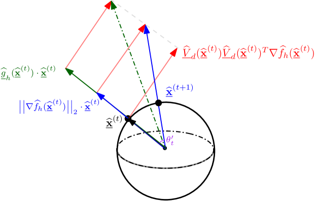
Figure 3: An illustration of one-step iterations under two candidate directional SCMS algorithms

$\bullet$ Method 2: The fixed-point iteration formula (34) of the directional mean shift algorithm suggests a more efficient formulation of the directional SCMS algorithm as:

$$\underline{\widehat{\bm{x}}}^{(t+1)}\leftarrow\underline{\widehat{\bm{x}}}^{(t)}+\widehat{\underline{V}}_{d}(\underline{\widehat{\bm{x}}}^{(t)})\widehat{\underline{V}}_{d}(\underline{\widehat{\bm{x}}}^{(t)})^{T}\cdot\frac{\nabla\widehat{f}_{h}(\underline{\widehat{\bm{x}}}^{(t)})}{\left|\left|\nabla\widehat{f}_{h}(\underline{\widehat{\bm{x}}}^{(t)})\right|\right|_{2}}\quad\text{ and }\quad\underline{\widehat{\bm{x}}}^{(t+1)}\leftarrow\frac{\underline{\widehat{\bm{x}}}^{(t+1)}}{\left|\left|\underline{\widehat{\bm{x}}}^{(t+1)}\right|\right|_{2}},$$ (39)

where we replace the directional mean shift vector $\underline{\Xi}_{h}(\bm{x})$ with the standardized total gradient estimator $\frac{\nabla\widehat{f}_{h}(\bm{x})}{\left|\left|\nabla\widehat{f}_{h}(\bm{x})\right|\right|_{2}}$ in (37). This directional SCMS is again a fixed-point iteration as:

$$\underline{\widehat{\bm{x}}}^{(t+1)}=\frac{\widehat{\underline{V}}_{d}(\underline{\widehat{\bm{x}}}^{(t)})\widehat{\underline{V}}_{d}(\underline{\widehat{\bm{x}}}^{(t)})^{T}\nabla\widehat{f}_{h}(\underline{\widehat{\bm{x}}}^{(t)})+\left|\left|\nabla\widehat{f}_{h}(\underline{\widehat{\bm{x}}}^{(t)})\right|\right|_{2}\cdot\underline{\widehat{\bm{x}}}^{(t)}}{\left|\left|\widehat{\underline{V}}_{d}(\underline{\widehat{\bm{x}}}^{(t)})\widehat{\underline{V}}_{d}(\underline{\widehat{\bm{x}}}^{(t)})^{T}\nabla\widehat{f}_{h}(\underline{\widehat{\bm{x}}}^{(t)})+\left|\left|\nabla\widehat{f}_{h}(\underline{\widehat{\bm{x}}}^{(t)})\right|\right|_{2}\cdot\underline{\widehat{\bm{x}}}^{(t)}\right|\right|_{2}}.$$ (40)

A direct computation demonstrates that, by the non-increasing property of kernel $L$ and the fact that $\left|\left|\bm{X}_{i}\right|\right|_{2}=1$ for $i=1,...,n$,

$$\begin{split}\left|\left|\nabla\widehat{f}_{h}(\bm{x})\right|\right|_{2}&=\left|\left|-\frac{c_{L,q}(h)}{nh^{2}}\sum_{i=1}^{n}\bm{X}_{i}L^{\prime}\left(\frac{1-\bm{x}^{T}\bm{X}_{i}}{h^{2}}\right)\right|\right|_{2}\\ &\leq\frac{c_{L,q}(h)}{nh^{2}}\sum_{i=1}^{n}\left|\left|\bm{X}_{i}L^{\prime}\left(\frac{1-\bm{x}^{T}\bm{X}_{i}}{h^{2}}\right)\right|\right|_{2}\\ &=-\frac{c_{L,q}(h)}{nh^{2}}\sum_{i=1}^{n}L^{\prime}\left(\frac{1-\bm{x}^{T}\bm{X}_{i}}{h^{2}}\right)=\widehat{\underline{g}}_{h}(\bm{x}).\end{split}$$ (41)

Because the radial components $\underline{\widehat{g}}_{h}(\underline{\widehat{\bm{x}}}^{(t)})\cdot\underline{\widehat{\bm{x}}}^{(t)}$ and $\left|\left|\nabla\widehat{f}_{h}(\underline{\widehat{\bm{x}}}^{(t)})\right|\right|_{2}\cdot\underline{\widehat{\bm{x}}}^{(t)}$ in directional SCMS iterative formulae (38) and (40) respectively make no contributions to the iteration of point $\underline{\widehat{\bm{x}}}^{(t)}$ on $\Omega_{q}$, the inequality (41) indicates that the directional SCMS algorithm with iterative formula (40) takes a larger step size in moving the SCMS sequence $\big{\{}\underline{\widehat{\bm{x}}}^{(t)}\big{\}}_{t=0}^{\infty}$ on $\Omega_{q}$. This helps accelerate the movements of those points that are far away from the ridge $\underline{\widehat{R}}_{d}$ or lie in the regions with low density values of $\widehat{f}_{h}$. In this sense, the directional SCMS algorithm with iterative formula (40) will be superior to (38); see Figure 3 for a graphical demonstration. We thus choose Method 2 as our directional SCMS algorithm. Algorithm 2 in Appendix A provides the detailed steps of implementing Method 2 in practice.

Inspired by Proposition 2 in Ghassabeh et al. (2013) for the Euclidean SCMS algorithm, we derive the ascending property of our directional SCMS algorithm (39) and two convergent results for stopping the algorithm in the following proposition. The proof is deferred to Appendix I, in which our argument is similar to but logically different from the proof of Proposition 2 in Ghassabeh et al. (2013).

Proposition 4.3.

Assume that the directional kernel $L$ is non-increasing, twice continuously differentiable, and convex with $L(0)<\infty$. Given the directional KDE $\widehat{f}_{h}(\bm{x})=\frac{c_{L,q}(h)}{n}\sum\limits_{i=1}^{n}L\left(\frac{1-\bm{x}^{T}\bm{X}_{i}}{h^{2}}\right)$ and the directional SCMS sequence $\big{\{}\underline{\widehat{\bm{x}}}^{(t)}\big{\}}_{t=0}^{\infty}\subset\Omega_{q}$ defined by (39) or (40), the following properties hold:

1. The estimated density sequence $\left\{\widehat{f}_{h}(\underline{\widehat{\bm{x}}}^{(t)})\right\}_{t=0}^{\infty}$ is non-decreasing and thus converges.

2. $\lim\limits_{t\to\infty}\left|\left|\widehat{\underline{V}}_{d}(\underline{\widehat{\bm{x}}}^{(t)})^{T}\nabla\widehat{f}_{h}(\underline{\widehat{\bm{x}}}^{(t)})\right|\right|_{2}=0$.

3. If the kernel $L$ is also strictly decreasing on $[0,\infty)$, then $\lim\limits_{t\to\infty}\left|\left|\underline{\widehat{\bm{x}}}^{(t+1)}-\underline{\widehat{\bm{x}}}^{(t)}\right|\right|_{2}=0$.

Remark 4.2.

Our results (b) and (c) in Proposition 4.3 demonstrates that the stopping criterion of our directional SCMS algorithm can follow either the norm of the principal Riemannian gradient estimator $\left|\left|\widehat{\underline{V}}_{d}(\underline{\widehat{\bm{x}}}^{(t)})^{T}\nabla\widehat{f}_{h}(\underline{\widehat{\bm{x}}}^{(t)})\right|\right|_{2}$ or the (Euclidean) distance $\left|\left|\underline{\widehat{\bm{x}}}^{(t+1)}-\underline{\widehat{\bm{x}}}^{(t)}\right|\right|_{2}$ between two consecutive iterative points, where the latter one requires a strictly decreasing kernel such as the von Mises kernel $L(r)=e^{-r}$.

Motivated by the iterative formula (35) for the gradient ascent algorithm on $\Omega_{q}$, we consider writing our directional SCMS algorithm as a variant of the SCGA algorithm on $\Omega_{q}$ with an iterative formula:

$$\widehat{\underline{\bm{x}}}^{(t+1)}=\mathtt{Exp}_{\widehat{\underline{\bm{x}}}^{(t)}}\left(\underline{\eta}_{n,h}^{(t)^{\prime}}\cdot\widehat{\underline{V}}_{d}(\widehat{\underline{\bm{x}}}^{(t)})\widehat{\underline{V}}_{d}(\widehat{\underline{\bm{x}}}^{(t)})^{T}\mathtt{grad}\,\widehat{f}_{h}(\widehat{\underline{\bm{x}}}^{(t)})\right),$$ (42)

where $\mathtt{Exp}_{\bm{x}}$ is the exponential map at $\bm{x}\in\Omega_{q}$ and $\underline{\eta}_{n,h}^{(t)^{\prime}}>0$ is the adaptive step size. Analogous to the Euclidean SCMS algorithm and its SCGA representation (22), the formulation (42) will reveal the (linear) convergence properties of our directional SCMS algorithm in the upcoming Section 4.3. To derive an explicit formula for $\underline{\eta}_{n,h}^{(t)^{\prime}}$, we recall the fixed-point equation (40) of our directional SCMS algorithm and compute the geodesic distance between $\underline{\widehat{\bm{x}}}^{(t+1)}$ and $\underline{\widehat{\bm{x}}}^{(t)}$ (one-step directional SCMS update) as:

$$\arccos\left(\left(\underline{\widehat{\bm{x}}}^{(t+1)}\right)^{T}\underline{\widehat{\bm{x}}}^{(t)}\right) =\arccos\left(\frac{\left|\left|\nabla\widehat{f}_{h}(\underline{\widehat{\bm{x}}}^{(t)})\right|\right|_{2}}{\left|\left|\underline{\widehat{V}}_{d}(\underline{\widehat{\bm{x}}}^{(t)})\underline{\widehat{V}}_{d}(\underline{\widehat{\bm{x}}}^{(t)})^{T}\nabla\widehat{f}_{h}(\underline{\widehat{\bm{x}}}^{(t)})+\left|\left|\nabla\widehat{f}_{h}(\underline{\widehat{\bm{x}}}^{(t)})\right|\right|_{2}\cdot\underline{\widehat{\bm{x}}}^{(t)}\right|\right|_{2}}\right)$$

$$=\left|\left|\underline{\eta}_{n,h}^{(t)^{\prime}}\cdot\underline{\widehat{V}}_{d}(\underline{\widehat{\bm{x}}}^{(t)})\underline{\widehat{V}}_{d}(\underline{\widehat{\bm{x}}}^{(t)})^{T}\mathtt{grad}\,\widehat{f}_{h}(\underline{\widehat{\bm{x}}}^{(t)})\right|\right|_{2},$$

where, in the second equality, we equate the geodesic distance between $\underline{\widehat{\bm{x}}}^{(t+1)}$ and $\underline{\widehat{\bm{x}}}^{(t)}$ to the norm of the tangent vector inside the exponential map in (42). This suggests that our directional SCMS algorithm is a (sample-based) SCGA algorithm on $\Omega_{q}$ with adaptive step size

$$\underline{\eta}_{n,h}^{(t)^{\prime}}=\frac{\arccos\left(\frac{\left|\left|\nabla\widehat{f}_{h}(\underline{\widehat{\bm{x}}}^{(t)})\right|\right|_{2}}{\left|\left|\underline{\widehat{V}}_{d}(\underline{\widehat{\bm{x}}}^{(t)})\underline{\widehat{V}}_{d}(\underline{\widehat{\bm{x}}}^{(t)})^{T}\nabla\widehat{f}_{h}(\underline{\widehat{\bm{x}}}^{(t)})+\left|\left|\nabla\widehat{f}_{h}(\underline{\widehat{\bm{x}}}^{(t)})\right|\right|_{2}\cdot\underline{\widehat{\bm{x}}}^{(t)}\right|\right|_{2}}\right)}{\left|\left|\underline{\widehat{V}}_{d}(\underline{\widehat{\bm{x}}}^{(t)})\underline{\widehat{V}}_{d}(\underline{\widehat{\bm{x}}}^{(t)})^{T}\nabla\widehat{f}_{h}(\underline{\widehat{\bm{x}}}^{(t)})\right|\right|_{2}}=\frac{\theta_{t}^{\prime}}{\left|\left|\nabla\widehat{f}_{h}(\underline{\widehat{\bm{x}}}^{(t)})\right|\right|_{2}\cdot\tan\theta_{t}^{\prime}}$$ (43)

for $t=0,1,...$, where $\theta_{t}^{\prime}$ denotes the angle between $\underline{\widehat{\bm{x}}}^{(t+1)}$ and $\underline{\widehat{\bm{x}}}^{(t)}$. Note that the above derivation is based on the orthogonality between $\underline{\widehat{\bm{x}}}^{(t)}$ and the order-$d$ principal Riemannian gradient estimator

$$\underline{\widehat{G}}_{d}(\underline{\widehat{\bm{x}}}^{(t)})=\underline{\widehat{V}}_{d}(\underline{\widehat{\bm{x}}}^{(t)})\underline{\widehat{V}}_{d}(\underline{\widehat{\bm{x}}}^{(t)})^{T}\mathtt{grad}\,\widehat{f}_{h}(\underline{\widehat{\bm{x}}}^{(t)})=\underline{\widehat{V}}_{d}(\underline{\widehat{\bm{x}}}^{(t)})\underline{\widehat{V}}_{d}(\underline{\widehat{\bm{x}}}^{(t)})^{T}\nabla\widehat{f}_{h}(\underline{\widehat{\bm{x}}}^{(t)});$$

see Figure 3 for a graphical illustration. When our directional SCMS algorithm approaches the estimated ridge $\underline{\widehat{R}}_{d}$, $\theta_{t}^{\prime}$ tends to 0 and $\frac{\theta_{t}^{\prime}}{\tan\theta_{t}^{\prime}}$ is approximately equal to 1. Thus, the step size $\underline{\eta}_{n,h}^{(t)^{\prime}}$ is also controlled by $\left|\left|\widehat{f}_{h}(\underline{\widehat{\bm{x}}}^{(t)})\right|\right|_{2}$ as in the directional mean shift scenario; see Equation (36). Therefore, Lemma 4.2 is still effective to argue that the step size $\underline{\eta}_{n,h}^{(t)^{\prime}}$ converges to 0 with probability tending to 1 when $h\to 0$ and $nh^{q}\to\infty$.

4.3 Linear Convergence of Population and Sample-Based SCGA Algorithms on $\Omega_{q}$

As we have shown in (42) that our proposed directional SCMS algorithm is an example of the sample-based SCGA method with directional KDE $\widehat{f}_{h}$ on $\Omega_{q}$ with an adaptive step size $\eta_{n,h}^{(t)^{\prime}}$, our main focus in this subsection will be on the (linear) convergence of such SCGA algorithm on $\Omega_{q}$. We first consider the population SCGA algorithm on $\Omega_{q}$ defined by its iterative formula as:

$$\underline{\bm{x}}^{(t+1)}=\mathtt{Exp}_{\underline{\bm{x}}^{(t)}}\left(\underline{\eta}\cdot\underline{V}_{d}(\underline{\bm{x}}^{(t)})\underline{V}_{d}(\underline{\bm{x}}^{(t)})^{T}\mathtt{grad}\,f(\underline{\bm{x}}^{(t)})\right)$$ (44)

with a suitable choice of the step size $\underline{\eta}>0$. The sample-based version substitutes the subspace constrained Riemannian gradient $\underline{V}_{d}(\underline{\bm{x}})\underline{V}_{d}(\underline{\bm{x}})^{T}\mathtt{grad}\,f(\underline{\bm{x}})$ with its estimator $\widehat{\underline{V}}_{d}(\underline{\bm{x}})\widehat{\underline{V}}_{d}(\underline{\bm{x}})^{T}\mathtt{grad}\,\widehat{f}_{h}(\underline{\bm{x}})$ and generally has a constant step size $\underline{\eta}>0$; see (42). In the sequel, we denote the sequence defined by the population SCGA algorithm with objective function $f$ on $\Omega_{q}$ by $\big{\{}\underline{\bm{x}}^{(t)}\big{\}}_{t=0}^{\infty}$ and the sequence defined by the sample-based SCGA algorithm with objective function $\widehat{f}_{h}$ on $\Omega_{q}$ by $\big{\{}\widehat{\underline{\bm{x}}}^{(t)}\big{\}}_{t=0}^{\infty}$.

Remark 4.3.

Note that the definition (44) of the SCGA algorithm is adaptive to any Riemannian manifold $\mathcal{M}$, not restricting to the unit hypersphere $\Omega_{q}$. The only requirement on $\mathcal{M}$ for (44) to be valid is that the exponential map $\mathtt{Exp}_{\underline{\bm{x}}^{(t)}}:T_{\bm{\underline{\bm{x}}^{(t)}}}(\mathcal{M})\to\mathcal{M}$ is well-defined within a small neighborhood of $\bm{0}$ on the tangent space $T_{\bm{\underline{\bm{x}}^{(t)}}}(\mathcal{M})$ for each $t\geq 0$. More importantly, our assumptions (A1-3) and condition (A4) are generalizable to any smooth function $f$ supported on $\mathcal{M}$, and our (linear) convergence results are applicable to the SCGA algorithm (44) on $\mathcal{M}$ whose sectional curvature is lower bounded by a real number; see one of the key lemmas in our proofs (Lemma I.1).

Similar to the SCGA algorithm in the Euclidean space $\mathbb{R}^{D}$, the following proposition demonstrates that the SCGA algorithm (44) on $\Omega_{q}$ yields a non-decreasing sequence of the objective function $f$ supported on $\Omega_{q}$ and a convergent SCGA sequence to the directional ridge $\underline{R}_{d}$, as long as the step size $\underline{\eta}$ is sufficiently small.

Proposition 4.4 (Convergence of the SCGA Algorithm on $\Omega_{q}$).

For any SCGA sequence $\big{\{}\underline{\bm{x}}^{(t)}\big{\}}_{t=0}^{\infty}\subset\Omega_{q}$ defined by (44) with $0<\underline{\eta}<\frac{2}{q\left|\left|\mathcal{H}f\right|\right|_{\infty}^{(2)}}$, the following properties hold:

1. Under condition (A1), the objective function sequence $\big{\{}f(\underline{\bm{x}}^{(t)})\big{\}}_{t=0}^{\infty}$ is non-decreasing and thus converges.

2. Under condition (A1), $\lim_{t\to\infty}\left|\left|\underline{V}_{d}(\underline{\bm{x}}^{(t)})^{T}\mathtt{grad}\,f(\underline{\bm{x}}^{(t)})\right|\right|_{2}=\lim_{t\to\infty}d_{g}\left(\underline{\bm{x}}^{(t+1)},\underline{\bm{x}}^{(t)}\right)=0$.

3. Under conditions (A1-3), $\lim_{t\to\infty}d_{g}\left(\underline{\bm{x}}^{(t)},\underline{R}_{d}\right)=0$ whenever $\underline{\bm{x}}^{(0)}\in\underline{R}_{d}\oplus\underline{r}_{1}$ with the convergence radius $\underline{r}_{1}$ satisfying

   $$0<\underline{r}_{1}<\min\left\{\underline{\rho}/2,\frac{\min\left\{\underline{\beta}_{1},1\right\}^{2}}{\underline{A}_{2}\left(\left|\left|f\right|\right|_{\infty}^{(3)}+\left|\left|f\right|\right|_{\infty}^{(4)}\right)},2\sin\left(\frac{\underline{\beta}_{1}}{2\underline{A}_{4}(f)}\right)\right\},$$

   where $\underline{A}_{2}$ is a constant defined in (h) of Lemma G.1 while $\underline{A}_{4}(f)>0$ is a quantity depending on both the dimension $q$ and the functional norm $\left|\left|f\right|\right|_{\infty,4}^{*}$ up to the fourth-order (partial) derivatives of $f$.

The proof of Proposition 4.4 can be found in Appendix I. The upper bound for the convergence radius $\underline{r}_{1}>0$ has the same meaning as in Proposition 3.3 for the Euclidean SCGA algorithm, ensuring that $\underline{r}_{1}\leq\mathtt{reach}(\underline{R}_{d})$ and the distances from the SCGA sequence $\big{\{}\underline{\bm{x}}^{(t)}\big{\}}_{t=0}^{\infty}$ on $\Omega_{q}$ to the directional ridge $\underline{R}_{d}$ can be upper bounded by the norms $\left|\left|\underline{V}_{d}(\underline{\bm{x}}^{(t)})^{T}\mathtt{grad}\,f(\underline{\bm{x}}^{(t)})\right|\right|_{2}$ of order-$d$ principal Riemannian gradients for all $t=0,1,...$.

Corollary 4.5 (Convergence of the Directional SCMS Algorithm).

When the fixed sample size $n$ is sufficiently large and the bandwidth $h$ is chosen to be correspondingly small, the following properties hold for the directional SCMS sequence $\big{\{}\widehat{\underline{\bm{x}}}^{(t)}\big{\}}_{t=0}^{\infty}\subset\Omega_{q}$ with high probability under conditions (A1-3) and (D1-2):

1. The directional KDE sequence $\left\{\widehat{f}_{h}(\widehat{\underline{\bm{x}}}^{(t)})\right\}_{t=0}^{\infty}$ is non-decreasing and thus converges.

2. $\lim_{t\to\infty}\left|\left|\widehat{\underline{V}}(\widehat{\underline{\bm{x}}}^{(t)})^{T}\mathtt{grad}\,\widehat{f}_{h}(\widehat{\underline{\bm{x}}}^{(t)})\right|\right|_{2}=\lim_{t\to\infty}d_{g}\left(\widehat{\underline{\bm{x}}}^{(t)},\widehat{\underline{\bm{x}}}^{(t+1)}\right)=0$.

3. $\lim_{t\to\infty}d_{g}\left(\widehat{\underline{\bm{x}}}^{(t)},\widehat{\underline{R}}_{d}\right)=0$ whenever $\widehat{\underline{\bm{x}}}^{(0)}\in\widehat{\underline{R}}_{d}\oplus\underline{r}_{1}$ with the convergence radius $\underline{r}_{1}>0$ defined in (c) of Proposition 4.4.

Corollary 4.5 should also be considered as the convergence results of the sample-based SCGA algorithm on $\Omega_{q}$. To justify Corollary 4.5, we know from Theorem 4.1 that conditions (A1-3) also hold with high probability for the directional KDE $\widehat{f}_{h}$ and its estimated directional ridge $\widehat{\underline{R}}_{d}$ when $\frac{nh^{q+6}}{|\log h|}$ is sufficiently large and $h$ is small enough. Further, by Lemma 4.2, the adaptive step size $\underline{\eta}_{n,h}^{(t)^{\prime}}$ of our directional SCMS algorithm can be smaller than the threshold value $\frac{2}{q\left|\left|\mathcal{H}f\right|\right|_{\infty}^{(2)}}$ in Proposition 4.4 but also universally bounded away from zero with respect to the iteration number $t$, given a sufficiently large but fixed sample $n$ and a sufficiently small bandwidth $h$; recall our Remark 3.2. As a result, Corollary 4.5 follows from Proposition 4.4. Notice that the statements in Proposition 4.3 are essentially the same as the results (a-b) in Corollary 4.5 here. However, similar to Proposition 2 in Ghassabeh et al. (2013) for the Euclidean SCMS algorithm, Proposition 4.3 for the directional SCMS algorithm is established under the convexity assumption on the directional kernel $L$ and holds for any sample size $n$ and bandwidth $h$. On the contrary, the results (a-b) in Corollary 4.5 are asymptotic and probabilistic properties, in which we require $\frac{nh^{q+6}}{|\log h|}\to\infty$ and $h\to 0$.

According to Proposition 4.4 and Corollary 4.5, we can denote the limiting points of the population and sample-based SCGA algorithms on $\Omega_{q}$ by $\underline{\bm{x}}^{*}\in\underline{R}_{d}$ and $\widehat{\underline{\bm{x}}}^{*}\in\widehat{\underline{R}}_{d}$, respectively. The definition of the linear convergence of any converging sequence on $\Omega_{q}$ (or an arbitrary Riemannian manifold) is similar to the one in the flat Euclidean space $\mathbb{R}^{D}$ (see Definition 3.5), except that the Euclidean distance is replaced with the geodesic distance on $\Omega_{q}$ in the definition; see Section 4.5 in Absil et al. (2008).

Using the notation in Zhang and Sra (2016), we let $\zeta(\kappa,c)\equiv\frac{\sqrt{|\kappa|}c}{\tanh(\sqrt{|\kappa|}c)}$. Given that the sectional curvature is $\kappa=1$ on $\Omega_{q}$, we have $\zeta(1,c)=\frac{c}{\tanh(c)}$. One can show by differentiating $\zeta(1,c)$ that $\zeta(1,c)$ is strictly increasing with respect to $c$ and $\zeta(1,c)>1$ for any $c>0$. Analogous to the Euclidean SCGA algorithms, we will establish the linear convergence of the SCGA sequence $\big{\{}\underline{\bm{x}}^{(t)}\big{\}}_{t=0}^{\infty}$ on $\Omega_{q}$ (or any Riemannian manifold whose sectional curvature is lower bounded by a real number) as well as its sample-based version under the following local condition.

• (A4) (Quadratic Behaviors of Residual Vectors) We assume that the SCGA sequence $\big{\{}\underline{\bm{x}}^{(t)}\big{\}}_{t=0}^{\infty}$ on $\Omega_{q}$ with step size $0<\underline{\eta}\leq\min\left\{\frac{4}{\underline{\beta}_{0}},\frac{1}{q\left|\left|\mathcal{H}f\right|\right|_{\infty}^{(2)}\cdot\zeta(1,\underline{\rho})}\right\}$ and $\underline{\bm{x}}^{*}\in\underline{R}_{d}$ as its limiting point satisfies

  $$\left\langle\underline{U}_{d}^{\perp}(\underline{\bm{x}}^{(t)})\mathtt{grad}\,f(\underline{\bm{x}}^{(t)}),\,\mathtt{Exp}_{\underline{\bm{x}}^{(t)}}^{-1}(\underline{\bm{x}}^{*})\right\rangle \leq\frac{\underline{\beta}_{0}}{4}\cdot d_{g}\left(\underline{\bm{x}}^{(t)},\underline{\bm{x}}^{*}\right)^{2},$$

  $$\left|\left|\underline{U}_{d}^{\perp}(\underline{\bm{x}}^{(t)})\mathtt{Exp}_{\underline{\bm{x}}^{(t)}}^{-1}(\underline{\bm{x}}^{*})\right|\right|_{2} \leq\underline{\beta}_{2}\cdot d_{g}\left(\underline{\bm{x}}^{(t)},\underline{\bm{x}}^{*}\right)^{2}$$

  for some constant $\underline{\beta}_{2}>0$, where $\underline{\beta}_{0}>0$ is the constant defined in condition (A2) and $\mathtt{Exp}_{\underline{\bm{x}}^{(t)}}^{-1}(\underline{\bm{x}}^{*})\in T_{\underline{\bm{x}}^{(t)}}$ is the logarithmic map.

Condition (A4) serves as a generalization of its Euclidean counterpart condition (A4) to $\Omega_{q}$, which again requires a quadratic behavior of the residual vector $\underline{U}_{d}^{\perp}(\underline{\bm{x}}^{(t)})\mathtt{Exp}_{\underline{\bm{x}}^{(t)}}^{-1}(\underline{\bm{x}}^{*})$ within the tangent space $T_{\underline{\bm{x}}^{(t)}}$. Under this condition, the objective (density) function $f$ is “subspace constrained geodesically strongly concave” around the directional ridge $\underline{R}_{d}$; see also Remark 4.4. Some discussions about potentially weaker assumptions that imply condition (A4) in Appendix E are also applicable in the manifold setting under some modifications; see Remark E.1. One intuitive example that condition (A4) holds is presented at the second row of Figure 5, where the directional SCMS/SCGA iterative vector $\mathtt{Exp}_{\underline{\bm{x}}^{(t)}}^{-1}(\underline{\bm{x}}^{*})$ is always orthogonal to the residual space $\underline{U}_{d}^{\perp}(\bm{x}^{(t)})$ for all $t\geq 0$ around the (estimated) ridge on $\Omega_{q}$.

Theorem 4.6 (Linear Convergence of the SCGA Algorithm on $\Omega_{q}$).

Assume conditions (A1-4) throughout the theorem.

1. Q-Linear convergence of $d_{g}(\underline{\bm{x}}^{(t)},\underline{\bm{x}}^{*})$: Consider a convergence radius $\underline{r}_{2}>0$ satisfying

   $$0<\underline{r}_{2} \leq\min\Bigg{\{}\underline{\rho}/2,\frac{\underline{\beta}_{1}^{2}}{\underline{A}_{2}\left(\left|\left|f\right|\right|_{\infty}^{(3)}+\left|\left|f\right|\right|_{\infty}^{(4)}\right)},\frac{\underline{\beta}_{1}}{\underline{A}_{4}(f)},$$

   $$2\sin\Bigg{[}\frac{3\underline{\beta}_{0}}{8q\left(12\left|\left|\mathcal{H}f\right|\right|_{\infty}^{(2)}\underline{\beta}_{2}^{2}\arcsin\left(\underline{\rho}/2\right)+\sqrt{q}\left|\left|f\right|\right|_{\infty}^{(3)}\right)}\Bigg{]}\Bigg{\}},$$

   where $\underline{A}_{2}>0$ is the constant defined in (h) of Lemma G.1 and $\underline{A}_{4}(f)>0$ is a quantity defined in (c) of Proposition 4.4 that depends on both the dimension $q$ and the functional norm $\left|\left|f\right|\right|_{\infty,4}^{*}$ up to the fourth-order (partial) derivatives of $f$. Whenever $0<\underline{\eta}\leq\min\left\{\frac{4}{\underline{\beta}_{0}},\frac{1}{q\left|\left|\mathcal{H}f\right|\right|_{\infty}^{(2)}\cdot\zeta(1,\underline{\rho})}\right\}$ and the initial point $\underline{\bm{x}}^{(0)}\in\text{Ball}_{q+1}(\underline{\bm{x}}^{*},\underline{r}_{2})\cap\Omega_{q}$ with $\underline{\bm{x}}^{*}\in\underline{R}_{d}$, we have that

   $$d_{g}(\underline{\bm{x}}^{(t)},\underline{\bm{x}}^{*})\leq\underline{\Upsilon}^{t}\cdot d_{g}(\underline{\bm{x}}^{(0)},\underline{\bm{x}}^{*})\quad\text{ with }\quad\underline{\Upsilon}=\sqrt{1-\frac{\underline{\beta}_{0}\underline{\eta}}{4}}.$$

2. R-Linear convergence of $d_{g}(\underline{\bm{x}}^{(t)},\underline{R}_{d})$: Under the same radius $\underline{r}_{2}>0$ in (a), we have that whenever $0<\underline{\eta}\leq\min\left\{\frac{4}{\underline{\beta}_{0}},\frac{1}{q\left|\left|\mathcal{H}f\right|\right|_{\infty}^{(2)}\cdot\zeta(1,\underline{\rho})}\right\}$ and the initial point $\underline{\bm{x}}^{(0)}\in\text{Ball}_{q+1}(\underline{\bm{x}}^{*},\underline{r}_{2})\cap\Omega_{q}$ with $\underline{\bm{x}}^{*}\in\underline{R}_{d}$,

   $$d_{g}(\underline{\bm{x}}^{(t)},\underline{R}_{d})\leq\underline{\Upsilon}^{t}\cdot d_{g}(\underline{\bm{x}}^{(0)},\underline{\bm{x}}^{*})\quad\text{ with }\quad\underline{\Upsilon}=\sqrt{1-\frac{\underline{\beta}_{0}\underline{\eta}}{4}}.$$

We further assume (D1-2) in the rest of statements. Suppose that $h\to 0$ and $\frac{nh^{q+4}}{|\log h|}\to\infty$.

1. Q-Linear convergence of $d_{g}(\widehat{\underline{\bm{x}}}^{(t)},\underline{\bm{x}}^{*})$: Under the same radius $\underline{r}_{2}>0$ and $\underline{\Upsilon}=\sqrt{1-\frac{\underline{\beta}_{0}\underline{\eta}}{4}}$ in (a), we have that

   $$d_{g}(\widehat{\underline{\bm{x}}}^{(t)},\underline{\bm{x}}^{*})\leq\underline{\Upsilon}^{t}\cdot d_{g}(\widehat{\underline{\bm{x}}}^{(0)},\underline{\bm{x}}^{*})+O(h^{2})+O_{P}\left(\sqrt{\frac{|\log h|}{nh^{q+4}}}\right)$$

   with probability tending to 1 whenever $0<\underline{\eta}\leq\min\left\{\frac{4}{\underline{\beta}_{0}},\frac{1}{q\left|\left|\mathcal{H}f\right|\right|_{\infty}^{(2)}\cdot\zeta(1,\underline{\rho})}\right\}$ and the initial point $\widehat{\underline{\bm{x}}}^{(0)}\in\text{Ball}_{q+1}(\underline{\bm{x}}^{*},\underline{r}_{2})\cap\Omega_{q}$ with $\underline{\bm{x}}^{*}\in\underline{R}_{d}$.

1. R-Linear convergence of $d_{g}(\widehat{\underline{\bm{x}}}^{(t)},\underline{R}_{d})$: Under the same radius $\underline{r}_{2}>0$ and $\underline{\Upsilon}=\sqrt{1-\frac{\underline{\beta}_{0}\underline{\eta}}{4}}$ in (a), we have that

   $$d_{g}(\widehat{\underline{\bm{x}}}^{(t)},\underline{R}_{d})\leq\underline{\Upsilon}^{t}\cdot d_{g}(\widehat{\underline{\bm{x}}}^{(0)},\underline{\bm{x}}^{*})+O(h^{2})+O_{P}\left(\sqrt{\frac{|\log h|}{nh^{q+4}}}\right)$$

   with probability tending to 1 whenever $0<\underline{\eta}\leq\min\left\{\frac{4}{\underline{\beta}_{0}},\frac{1}{q\left|\left|\mathcal{H}f\right|\right|_{\infty}^{(2)}\cdot\zeta(1,\underline{\rho})}\right\}$ and the initial point $\widehat{\underline{\bm{x}}}^{(0)}\in\text{Ball}_{q+1}(\underline{\bm{x}}^{*},\underline{r}_{2})\cap\Omega_{q}$ with $\underline{\bm{x}}^{*}\in\underline{R}_{d}$.

The detailed proof of Theorem 4.6 is in Appendix I. The theorem illuminates both the step size requirement and the convergence radius $\underline{r}_{2}>0$ for the linear convergence of SCGA algorithms on $\Omega_{q}$. Similar to Euclidean SCGA algorithms in Theorem 3.6, the upper bound of the convergence radius $\underline{r}_{2}$ consists of the three quantities adopted from Proposition 4.4 and a quantity controlling the “subspace constrained geodesically strong concavity” around the directional ridge $\underline{R}_{d}$.

Remark 4.4.

Similar to Euclidean SCGA algorithms, the geodesically strong concavity assumption (Zhang and Sra, 2016) on the objective function $f$ is not sufficient to prove the linear convergence of the SCGA algorithm (44) on $\Omega_{q}$. We instead establish the following “subspace constrained geodesically strong concavity” under some mild conditions (A1-4):

$$f(\underline{\bm{x}}^{*})-f(\bm{y})\leq\left\langle\underline{V}_{d}(\bm{y})\underline{V}_{d}(\bm{y})^{T}\mathtt{grad}\,f(\bm{y}),\mathtt{Exp}_{\bm{y}}^{-1}(\underline{\bm{x}}^{*})\right\rangle-A_{8}\cdot d_{g}(\underline{\bm{x}}^{*},\bm{y})^{2}+o\left(d_{g}(\underline{\bm{x}}^{*},\bm{y})^{2}\right)$$ (45)

for some constant $A_{8}>0$, where $\bm{y}$ is generally chosen to be $\underline{\bm{x}}^{(t)}$. In fact, the most critical factors for establish this property is the eigengap condition (A2) and the quadratic behaviors of residual vectors stated in condition (A4).

Corollary 4.7 (Linear Convergence of the Directional SCMS Algorithm).

Assume conditions (A1-4) and (D1-2). When the fixed sample size $n$ is sufficiently large and the fixed bandwidth is chosen to be sufficiently small, there exists a convergence radius $\underline{r}_{3}\in\left(0,\underline{r}_{2}\right)$ such that the directional SCMS sequence $\left\{\widehat{\underline{\bm{x}}}^{(t)}\right\}_{t=0}^{\infty}$ satisfies

$$d_{g}\left(\widehat{\underline{\bm{x}}}^{(t)},\widehat{\underline{R}}_{d}\right)\leq d_{g}\left(\widehat{\underline{\bm{x}}}^{(t)},\widehat{\underline{\bm{x}}}^{*}\right)\leq\underline{\Upsilon}_{n,h}^{t}\cdot d_{g}\left(\widehat{\underline{\bm{x}}}^{(t)},\widehat{\underline{\bm{x}}}^{*}\right)$$

$$\text{ with }\quad\underline{\Upsilon}_{n,h}=\sqrt{1-\frac{\underline{\beta}_{0}\widetilde{\underline{\eta}}_{n,h}}{4}}\text{ and }\widetilde{\underline{\eta}}_{n,h}=\inf_{t}\underline{\eta}_{n,h}^{(t)^{\prime}}$$

with high probability whenever $0<\sup_{t}\underline{\eta}_{n,h}^{(t)^{\prime}}\leq\min\left\{\frac{4}{\underline{\beta}_{0}},\frac{1}{q\left|\left|\mathcal{H}f\right|\right|_{\infty}^{(2)}\cdot\zeta(1,\underline{\rho})}\right\}$ and the initial point $\widehat{\underline{\bm{x}}}^{(0)}\in\left(\widehat{\underline{R}}_{d}\oplus\underline{r}_{3}\right)\cap\Omega_{q}$.

We also identify Corollary 4.7 as the linear convergence of the sample-based SCGA algorithm on $\Omega_{q}$ to the estimated directional ridge $\widehat{\underline{R}}_{d}$ defined by the directional KDE $\widehat{f}_{h}$. The corollary can be justified by noticing that, under conditions (D1-2) and the uniform bounds (32), $\widehat{f}_{h}$ satisfies conditions (A1-3) with probability tending to 1 as $h\to 0$ and $\frac{nh^{q+6}}{|\log h|}\to\infty$; see Theorem 4.1. With this fact, one can leverage our argument in (a) of Theorem 4.6 to prove the linear convergence of the sample-based SCGA algorithm on $\Omega_{q}$ with a fixed step size $\underline{\eta}$ satisfying $0<\underline{\eta}\leq\min\left\{\frac{4}{\underline{\beta}_{0}},\frac{1}{q\left|\left|\mathcal{H}f\right|\right|_{\infty}^{(2)}\cdot\zeta(1,\underline{\rho})}\right\}$. Additionally, when the fixed sample size $n$ is sufficiently large and the bandwidth is chosen to be accordingly small, the adaptive step size $\underline{\eta}_{n,h}^{(t)^{\prime}}$ of our directional SCMS algorithm in (43) always falls below the threshold value $\min\left\{\frac{4}{\underline{\beta}_{0}},\frac{1}{q\left|\left|\mathcal{H}f\right|\right|_{\infty}^{(2)}\cdot\zeta(1,\underline{\rho})}\right\}$ for linear convergence by Lemma 4.2 but is also bounded away from zero; recall Remark 3.2. Taking the infimum of $\underline{\eta}_{n,h}^{(t)^{\prime}}$ with respect to the iteration number $t$ under a fixed $n$ and $h$ yields our results in Corollary 4.7.

5 Experiments

In this section, we first validate our linear convergence results of both Euclidean and directional SCMS algorithms on some simulated datasets. Then, we apply these two algorithms to a real-world earthquake dataset so as to identify its density ridges and compare the estimated ridges with boundaries of tectonic plates and fault lines, on which earthquakes are known to happen frequently.

We leverage the Gaussian kernel profile $k_{N}(x)=\exp\left(-\frac{x}{2}\right)$ in the Euclidean SCMS algorithm and the von Mises kernel $L(r)=e^{-r}$ in the directional SCMS algorithm. In addition, the logarithms of the estimated densities are utilized in our actual implementations (Step 2 in Algorithms 1 and 2 in Appendix A) of the Euclidean and directional SCMS algorithms because of two advantages. First, using the log-density in the Euclidean SCMS algorithm leads to a faster convergence process (Ghassabeh et al., 2013); see our empirical illustration in Figure 7. Second, estimating a hidden manifold with a density ridge defined by a log-density stabilizes the valid region for a well-defined ridge compared to the corresponding ridge defined by the original density; see Theorem 7 (Surrogate theorem) in Genovese et al. (2014).

Unless stated otherwise, we set the default bandwidth parameter of the Euclidean SCMS algorithm to the normal reference rule in Chacón et al. (2011); Chen et al. (2016), which is

$$h_{\text{NR}}=\bar{S}_{n}\times\left(\frac{4}{D+4}\right)^{\frac{1}{D+6}}n^{-\frac{1}{D+6}},\quad\bar{S}_{n}=\frac{1}{D}\sum_{j=1}^{D}S_{n,j},$$ (46)

where $S_{n,j}$ is the sample standard deviation along $j$-th coordinate and $D$ is the (Euclidean) dimension of the data in $\mathbb{R}^{D}$. As mentioned by Chen et al. (2016), there are two advantages of applying the normal reference rule (46) in our context. First, the KDE $\widehat{p}_{n}$ under $h_{\text{NR}}$ tends to be oversmoothing (Sheather, 2004), because the bandwidth minimizes the asymptotic MISE for estimating the first-order derivatives of a multivariate Gaussian distribution with covariance matrix $\sigma^{2}\bm{I}_{D}$; see Corollary 4 in Chacón et al. (2011). More importantly, the Euclidean SCMS algorithm with an oversmoothed KDE $\widehat{p}_{n}$ would not produce too many spurious ridges. Second, compared to cross validation methods, $h_{\text{NR}}$ is easy to compute in practice, especially when the dimension of data is high. The default bandwidth parameter of the directional SCMS algorithm is selected via the rule of thumb in Proposition 2 of García-Portugués (2013), which optimizes the asymptotic MISE for a $\text{vMF}(\bm{\mu},\nu)$ distribution. The concentration parameter $\nu$ is estimated by Equation (4.4) in Banerjee et al. (2005). That is,

$$h_{\text{ROT}}=\left[\frac{4\pi^{\frac{1}{2}}\mathcal{I}_{\frac{q-1}{2}}(\widehat{\nu})^{2}}{\widehat{\nu}^{\frac{q+1}{2}}\left[2q\cdot\mathcal{I}_{\frac{q+1}{2}}(2\widehat{\nu})+(q+2)\widehat{\nu}\cdot\mathcal{I}_{\frac{q+3}{2}}(2\widehat{\nu})\right]n}\right]^{\frac{1}{q+4}},\quad\widehat{\nu}=\frac{\bar{R}(q+1-\bar{R})}{1-\bar{R}^{2}},$$ (47)

where $\bar{R}=\frac{\left|\left|\sum_{i=1}^{n}\bm{X}_{i}\right|\right|_{2}}{n}$ given the directional dataset $\left\{\bm{X}_{1},...,\bm{X}_{n}\right\}\subset\Omega_{q}\subset\mathbb{R}^{q+1}$ and we recall that $\mathcal{I}_{\alpha}(\nu)$ is the modified Bessel function of the first kind of order $\nu$. As $q$-von Mises-Fisher distribution behaves as the Gaussian distribution on $\Omega_{q}$, choosing the bandwidth (47) also helps smooth out the resulting directional KDE. The tolerance level is always set to be $\epsilon=10^{-9}$ for any SCMS algorithm.

5.1 Simulation Study on the Euclidean SCMS Algorithm

To evaluate the algorithmic rate of convergence of the Euclidean SCMS algorithm (Algorithm 1), we generate the first simulated dataset by randomly drawing 1000 data points from a Gaussian mixture model with density $0.4\cdot N(\bm{\mu}_{1},\Sigma_{1})+0.6\cdot N(\bm{\mu}_{2},\Sigma_{2})$, where $\bm{\mu}_{1}=-\bm{\mu}_{2}=(1,1)^{T}$, $\Sigma_{1}=\mathtt{Diag}\left(\frac{1}{4},\frac{1}{4}\right)$, and $\Sigma_{2}=\begin{pmatrix}\frac{1}{2}&\frac{1}{4}\\ \frac{1}{4}&\frac{1}{2}\end{pmatrix}$. Another simulated dataset consists of 1000 data points randomly generated from an upper half circle with radius 2 and i.i.d. Gaussian noises $N(0,0.3^{2})$. When applying Algorithm 1 with the estimated log-density on each of these two simulated datasets, we choose the set of initial mesh points as the simulated dataset itself and remove those initial points whose density values are below 25% of the maximum density from the set of mesh points in order to obtain a cleaner ridge structure.

Figure 4 presents the Euclidean KDE plots, estimated density ridges from the Euclidean SCMS algorithm, and their (linear) convergence plots on the two simulated datasets. The linear trends of those plots in the second and third columns of Figure 4 empirically demonstrate the correctness of our Theorem 3.6 and Corollary 3.7 about the linear convergence of the Euclidean SCMS algorithm.

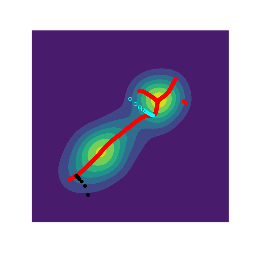
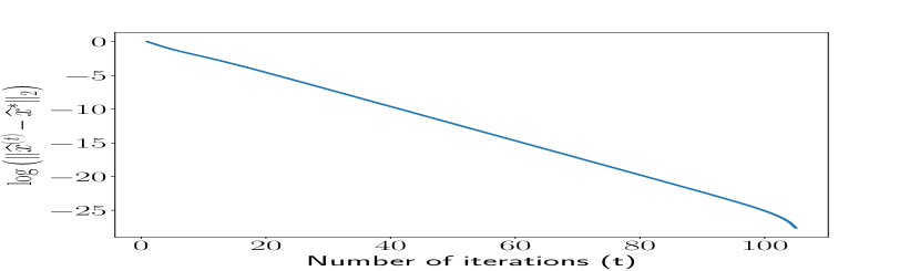
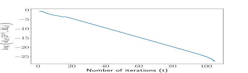
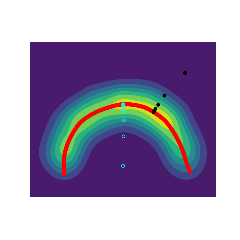
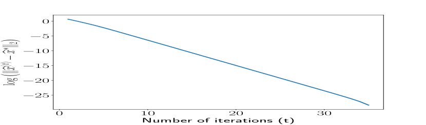
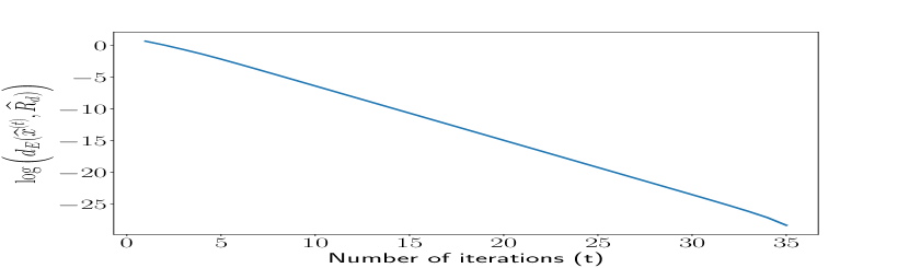
Figure 4: Density ridges estimated by the Euclidean SCMS algorithm on the two simulated datasets and their (linear) convergence plots. Horizontally, the first row displays the results of the simulated Gaussian mixture dataset, while the second row presents the results of the half circle simulated dataset. Vertically, the first column includes plots with Euclidean KDE, estimated ridges, and trajectories of SCMS sequences from two (randomly) chosen initial points. The second and third columns present the (linear) convergence plots for the log-distances of points in the highlighted sequences (indicated by hollow cyan points) to their limiting points or the estimated ridges.

5.2 Simulation Study on the Directional SCMS Algorithm

Analogous to our simulation study for the linear convergence of the Euclidean SCMS algorithm, we verify the linear convergence of our directional SCMS algorithm (Algorithm 2) on two different simulated datesets. One of them comprises 1000 data points randomly generated from a vMF mixture model $0.4\cdot\text{vMF}\left(\underline{\bm{\mu}}_{1},\nu_{1}\right)+0.6\cdot\text{vMF}\left(\underline{\bm{\mu}}_{2},\nu_{2}\right)$ with $\underline{\bm{\mu}}_{1}=(0,0,1)^{T}\in\Omega_{2}\subset\mathbb{R}^{3}$, $\underline{\bm{\mu}}_{2}=(1,0,0)^{T}\in\Omega_{2}\subset\mathbb{R}^{3}$, and $\nu_{1}=\nu_{2}=10$. The other simulated dataset is identical to the example in the right panel of Figure 1 and the underlying dataset in Figure 9, which consists of 1000 randomly sampled points from a circle connecting two poles on $\Omega_{2}$ with i.i.d. additive Gaussian noises $N(0,0.2^{2})$ to their Cartesian coordinates and additional $L_{2}$ normalization onto $\Omega_{2}$. In our implementation of Algorithm 2 with the directional log-density on the two simulated datasets, we also set each initial mesh as the dataset itself and remove those points whose density values are below 10% of the maximal density value from each set of mesh points.

Figure 5 shows the directional KDE plots, estimated density ridges on $\Omega_{2}$ from the directional SCMS algorithm, and their (linear) convergence plots on the aforementioned simulated datasets. Those linear decreasing trends in the convergence plots, possibly after several pilot iterations, illustrate the locally linear convergence of the directional SCMS algorithm that we proved in Theorem 4.6 and Corollary 4.7. Note that those minor perturbations at the tails of some linear convergence plots in Figure 5 are due to precision errors.

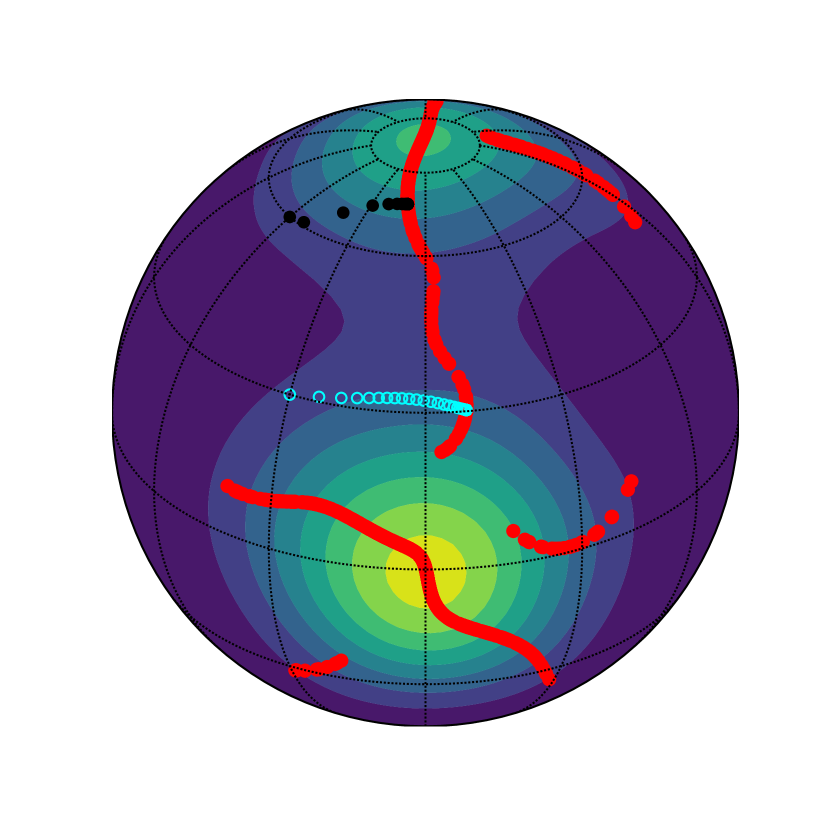
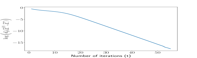
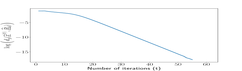
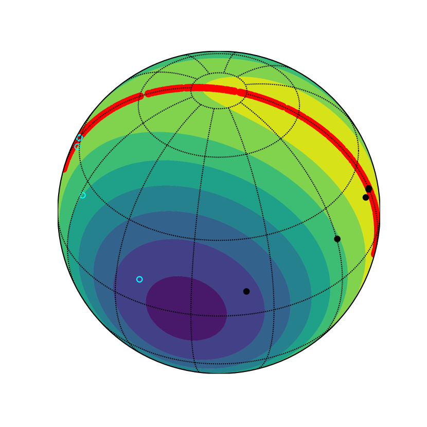
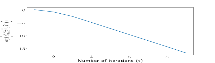
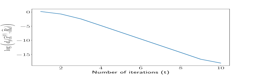
Figure 5: Density ridges estimated by the directional SCMS algorithm performed on the two simulated datasets and their (linear) convergence plots. Horizontally, the first row displays the results on the simulated vMF mixture dataset, while the second row presents the results on the circular simulated dataset on $\Omega_{2}$. Vertically, the first column includes plots with directional KDE, estimated ridges, and trajectories of directional SCMS sequences from two (randomly) chosen initial points on $\Omega_{2}$. The second and third columns present the convergence plots for the log-distances of points in the highlighted sequences (indicated by hollow cyan points) to their limiting points or the estimated ridges on $\Omega_{2}$.

5.3 Density Ridges on Earthquake Data

It is well-known that earthquakes on Earth tend to strike more frequently along the boundaries of tectonic plates and fault lines (i.e., sections of a plate or two plates are moving in different directions); see Subarya et al. (2006); Harris (2017) for more details. We analyze earthquakes with magnitudes of 2.5+ occurring between 2020-10-01 00:00:00 UTC and 2021-03-31 23:59:59 UTC, which can be obtained from the Earthquake Catalog (https://earthquake.usgs.gov/earthquakes/search/) of the United States Geological Survey. The dataset $\mathcal{D}$ contains 15049 earthquakes worldwide in this half-year period.

The normal reference rule (46) leads to the bandwidth parameter $h_{\text{NR}}\approx 16.0035$ and the rule of thumb (47) yields $h_{\text{ROT}}\approx 0.1584$ under the earthquake dataset $\mathcal{D}$. However, as these bandwidths lead to oversmoothing density estimates, we decrease the bandwidths for the Euclidean and directional SCMS algorithms to $h_{\text{Eu}}=7.0$ and $h_{\text{Dir}}=0.1$ respectively in order to detect more ridge structures. We generate 5000 points uniformly on the sphere $\Omega_{2}$ as the initial mesh points.

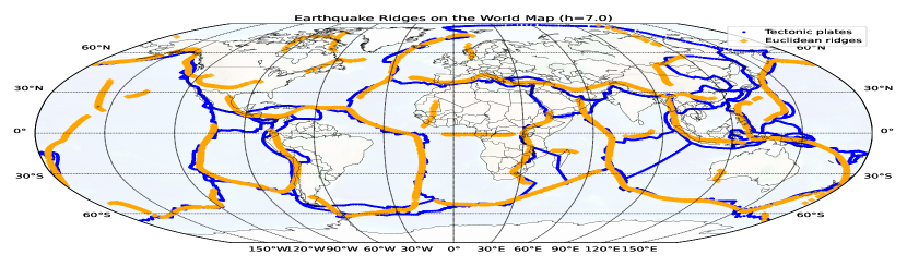
(a) Estimated ridges via Euclidean SCMS

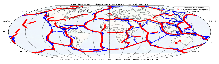
(b) Estimated ridges via directional SCMS

Figure 6: Comparisons between density ridges obtained by the Euclidean SCMS algorithm on angular coordinates and the directional SCMS algorithm on Cartesian coordinates from the earthquake dataset. On each panel, the ground-truth boundaries of tectonic plates are plots in blue curves.

To compare the earthquake ridges obtained by the Euclidean and directional SCMS algorithms with the boundaries of tectonic plates, we download the boundary geometry file of the 56 tectonic plates from https://www.kaggle.com/cwthompson/tectonic-plate-boundaries according to the models of Bird (2003); Argus et al. (2011) and overlap them with the estimated ridges in Figure 6. The results suggest that the ridges identified by the Euclidean and directional SCMS algorithms on the earthquake dataset coincide with the boundaries of tectonic plates to a large extent. Note that the Euclidean and directional ridges on the earthquake dataset $\mathcal{D}$ do not show too much difference, because most of the observed earthquakes are in the low latitude region ($\leq 60^{\circ}$) where most human beings live. Yet, the ridges estimated by our proposed directional SCMS algorithm do align better with the boundary of the Eurasian Plate near the North Pole than the ones estimated by the Euclidean SCMS algorithm, which confirms the superiority of our directional SCMS algorithm in the high latitude region; see also Appendix B for more in-depth analysis.

We further quantify the performances of earthquake ridges $\widehat{R}_{1}$ and $\underline{\widehat{R}}_{1}$ estimated by the Euclidean and directional SCMS algorithms from two different perspectives. First, given the fact that an estimated ridge should lie on the region where earthquakes happen more intensively, we compute the mean geodesic distances from each point in the earthquake dataset $\mathcal{D}$ to the ridges $\widehat{R}_{1}$ and $\underline{\widehat{R}}_{1}$ respectively as:

$$\frac{1}{|\mathcal{D}|}\sum_{\bm{x}\in\mathcal{D}}d_{g}(\bm{x},\widehat{R}_{1})\approx 0.02241\quad\text{ and }\quad\frac{1}{|\mathcal{D}|}\sum_{\bm{x}\in\mathcal{D}}d_{g}(\bm{x},\underline{\widehat{R}}_{1})\approx 0.02150,$$

where $|\mathcal{D}|=15049$ is the number of earthquakes in the dataset. The ridge $\underline{\widehat{R}}_{1}$ estimated by our directional SCMS algorithm is around 4% closer to the earthquakes in $\mathcal{D}$ on average. Second, we assess the estimation errors of $\widehat{R}_{1}$ and $\underline{\widehat{R}}_{1}$ with respect to the boundaries of tectonic plates. To this end, we view the surface of the Earth as a unit sphere $\Omega_{2}$ and define a manifold-recovering error measure (Zhang and Chen, 2021c) between the set of boundary points $\mathcal{B}$ and an estimated ridge $\widehat{R}$ as:

$$d_{E}\left(\mathcal{B},\widehat{R}\right)=\frac{1}{2}\left[\frac{1}{|\widehat{R}|}\sum_{\bm{x}\in\widehat{R}}d_{g}(\bm{x},\mathcal{B})+\frac{1}{|\mathcal{B}|}\sum_{\bm{y}\in\mathcal{B}}d_{g}(\bm{y},\widehat{R})\right],$$ (48)

where $|\widehat{R}|$ and $|\mathcal{B}|$ are the cardinalities of $\widehat{R}$ and $\mathcal{B}$, respectively. Note that although the density ridge $\widehat{R}$ and the boundaries of tectonic plates $\mathcal{B}$ are continuous structures in theory, they are generally represented by sets of discrete points in practice. That is why we can calculate their cardinalities without computing complicated integrals. Moreover, the manifold-recovering error measure is an average between the mean geodesic distances from each point in $\widehat{R}$ to $\mathcal{B}$ and from each point in $\mathcal{B}$ to $\widehat{R}$. We define such a balanced error measure to avoid biasing toward an estimated ridge $\widehat{R}$ that only approximates a small portion of $\mathcal{B}$ in high accuracy but fails to cover other parts of $\mathcal{B}$; see Figure 4 in Zhang and Chen (2021c) for an illustrative example. The manifold-recovering error measures of the ridges $\widehat{R}_{1}$ and $\underline{\widehat{R}}_{1}$ estimated by the Euclidean and directional SCMS algorithms with respect to the boundaries of tectonic plates $\mathcal{B}$ are

$$d_{E}\left(\mathcal{B},\widehat{R}_{1}\right)\approx 0.05332\quad\text{ and }\quad d_{E}\left(\mathcal{B},\underline{\widehat{R}}_{1}\right)\approx 0.05121.$$

Our directional SCMS algorithm again reduces the estimation error by around 3.9%. In summary, the earthquake ridges yielded by our directional SCMS algorithm are not only closer to the earthquakes on average than the ones identified by the Euclidean SCMS algorithm but also have a lower error in approximating the boundaries of tectonic plates.

6 Discussions

In this paper, we have provided a rigorous proof for the linear convergence of the well-known SCMS algorithm by viewing it as an example of the SCGA algorithm. We have also generalized the definition of density ridges from the usual densities supported on compact sets in $\mathbb{R}^{D}$ to the directional densities supported on $\Omega_{q}$ with nonzero curvature. The stability theorem of directional density ridges has been established, and the linear convergence of our proposed directional SCMS algorithm has been proved. Table 1 summarizes the frameworks of considering the (directional) mean shift/SCMS algorithms as gradient ascent/SCGA methods (on $\Omega_{q}$) and our results of asymptotic convergence rates of their corresponding step sizes.

Table 1: Comparisons between the Euclidean and directional mean shift (MS) or SCMS algorithms and summary of the asymptotic convergence rates of their adaptive sizes when viewed as GA/SCGA algorithms in $\mathbb{R}^{D}$ or on $\Omega_{q}$.

Algorithms	Recast forms as GA/SCGA (in $\mathbb{R}^{D}$ or on $\Omega_{q}$)	Asymptotic step sizes
	$\widehat{\bm{x}}^{(t+1)}\leftarrow\begin{cases}\widehat{\bm{x}}^{(t)}+\eta_{n,h}^{(t)}\cdot\nabla\widehat{p}_{n}(\widehat{\bm{x}}^{(t)})\\ \widehat{\bm{x}}^{(t)}+\eta_{n,h}^{(t)}\cdot\widehat{V}_{d}(\widehat{\bm{x}}^{(t)})\widehat{V}_{d}(\widehat{\bm{x}}^{(t)})^{T}\nabla\widehat{p}_{n}(\widehat{\bm{x}}^{(t)})\end{cases}$	$\eta_{n,h}^{(t)}\asymp O(h^{2})+o_{P}(h^{2})$
MS / SCMS in $\mathbb{R}^{D}$		(See Lemma 3.2)
	$\widehat{\underline{\bm{x}}}^{(t+1)}\leftarrow\begin{cases}\mathtt{Exp}_{\widehat{\underline{\bm{x}}}^{(t)}}\left(\underline{\eta}_{n,h}^{(t)}\cdot\mathtt{grad}\,\widehat{f}_{h}(\widehat{\underline{\bm{x}}}^{(t)})\right)\\ \mathtt{Exp}_{\widehat{\underline{\bm{x}}}^{(t)}}\left(\underline{\eta}_{n,h}^{(t)^{\prime}}\cdot\widehat{\underline{V}}_{d}(\widehat{\underline{\bm{x}}}^{(t)})\widehat{\underline{V}}_{d}(\widehat{\underline{\bm{x}}}^{(t)})^{T}\mathtt{grad}\,\widehat{f}_{h}(\widehat{\underline{\bm{x}}}^{(t)})\right)\end{cases}$	$\underline{\eta}_{n,h}^{(t)}\asymp\underline{\eta}_{n,h}^{(t)^{\prime}}$
MS /		$\quad=O(h^{2})+o_{P}(h^{2}),$
SCMS on $\Omega_{q}$		(See Lemma 4.2)

Our theoretical analyses of the SCGA algorithm in the Euclidean space $\mathbb{R}^{D}$ and on the unit hypersphere $\Omega_{q}$ has potential implications beyond proving the linear convergence of SCMS algorithms. In the optimization literature (Nocedal and Wright, 2006; Absil et al., 2008; Zhang and Sra, 2016; Nesterov et al., 2018), it is well-known that a standard gradient ascent method (on a smooth manifold) will converge linearly given an appropriate step size when the objective function is smooth and (geodesically) strongly concave. However, as we have discussed in Remarks 3.3 and 4.4, the smoothness and (geodesically) strong concavity assumptions are not sufficient for the linear convergence of the SCGA algorithms. Therefore, identifying density ridges with the SCGA algorithms is not only a nonconvex optimization problem, but also fundamentally more complex than standard gradient ascent methods. The assumptions and proof arguments developed in this paper may give some insights into the linear convergence of the SCGA algorithms with other forms of subspace constrained gradients.

There are still many open problems related to the SCMS algorithm. First, a central issue in determining the performance of a SCMS algorithm is the bandwidth selection. There is a variety of bandwidth selection mechanisms available to the Euclidean KDE and its derivatives in the literature (Chacón et al., 2011; Scott, 2015), but it is unclear how they can be applied to the SCMS algorithm. We plan to specialize or generalize such techniques to the SCMS algorithm under both the Euclidean and directional data. Second, our definition of density ridges is generalizable to any density supported on an arbitrary Riemannian manifold. As Hauberg (2015) has formulated the principal curve on a Riemannian manifold based on its classical definition in Hastie and Stuetzle (1989), it will be interesting to propose a new definition of principal curves from the perspective of density ridges on Riemannian manifolds and derive a more general SCMS algorithm, possibly based on some existing nonlinear mean shift methods on manifolds (Subbarao and Meer, 2006, 2009).

Appendix A Algorithmic Summaries of Euclidean and Directional SCMS Algorithms

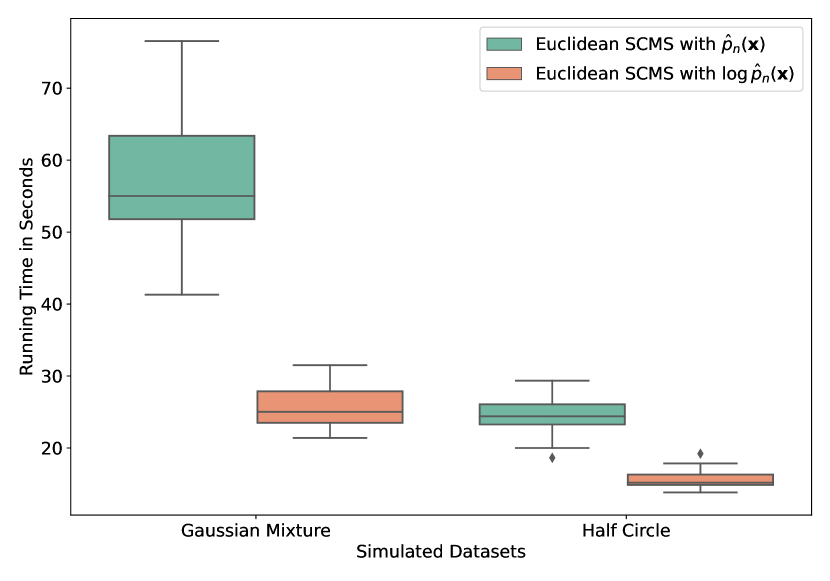
(a) Repeated experiments with the simulated Euclidean datasets in Figure 4.

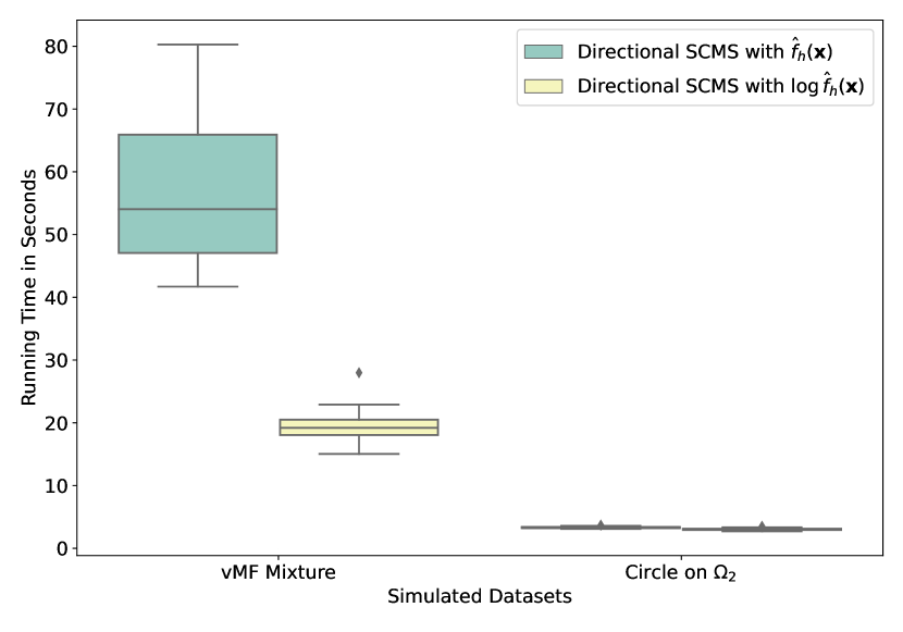
(b) Repeated experiments with the simulated directional datasets in Figure 5.

Figure 7: Running time comparisons between the (directional) SCMS algorithms with the original density and the log-density applied to our simulated datasets in Figures 4 and 5.

In this section, we provide algorithmic summaries of the Euclidean and directional SCMS algorithms for practical reference. Algorithm 1 describes each step of the Euclidean SCMS algorithm in detail. In our actual implementation of the algorithm, we replace the density estimator $\widehat{p}_{n}(\bm{x})$ with $\log\widehat{p}_{n}(\bm{x})$. To demonstrate that the (directional) SCMS algorithms under the log-density implementation give rise to a faster convergence process, we repeat our experiments in Sections 5.1 and 5.2 (i.e., Figures 4 and 5) 20 times for each simulated dataset with the (directional) SCMS algorithms under the original (estimated) density and the (estimated) log-density, respectively. The comparisons between their running times are shown in Figure 7, in which the (directional) SCMS algorithms under the log-density implementation clearly outperform their counterparts with the original density in terms of the average elapsed time until convergence.

Additionally, when the observational data in practice are noisy, it is common to incorporate an extra denoising step before Step 2 of Algorithm 1 to remove observations in low-density areas and stabilize the (Euclidean) SCMS algorithm; see Genovese et al. (2014); Chen et al. (2015b) for comparative studies that demonstrate the significance of denoising.

Algorithm 1 (Euclidean) Subspace Constrained Mean Shift (SCMS) Algorithm

Input:

• A data sample $\bm{X}_{1},...,\bm{X}_{n}\sim p(\bm{x})$ in $\mathbb{R}^{D}$.

• The order $d$ of the ridge, smoothing bandwidth $h>0$, and tolerance level $\epsilon>0$.

• A suitable mesh $\mathbb{M}_{E}\subset\mathbb{R}^{D}$ of initial points. By default, $\mathbb{M}_{E}=\left\{\bm{X}_{1},...,\bm{X}_{n}\right\}$.

Step 1: Compute the density estimator $\widehat{p}_{n}(\bm{x})=\frac{c_{k,D}}{nh^{D}}\sum\limits_{i=1}^{n}k\left(\left|\left|\frac{\bm{x}-\bm{X}_{i}}{h}\right|\right|_{2}^{2}\right)$ on the mesh $\mathbb{M}_{E}$.

Step 2: For each initial point $\widehat{\bm{x}}^{(0)}\in\mathbb{M}_{E}$, iterate the following SCMS update until convergence:

while $\left|\left|\widehat{V}_{d}(\widehat{\bm{x}}^{(t)})^{T}\nabla\widehat{p}_{n}(\widehat{\bm{x}}^{(t)})\right|\right|_{2}>\epsilon$ do

     Step 2-1: Compute the estimated Hessian matrix as:

$$\begin{split}\nabla\nabla\widehat{p}_{n}(\widehat{\bm{x}}^{(t)})=\frac{c_{k,D}}{nh^{D+2}}\sum_{i=1}^{n}&\Bigg{[}2\bm{I}_{D}\cdot k^{\prime}\left(\left|\left|\frac{\widehat{\bm{x}}^{(t)}-\bm{X}_{i}}{h}\right|\right|_{2}^{2}\right)\\ &\quad+\frac{4}{h^{2}}(\widehat{\bm{x}}^{(t)}-\bm{X}_{i})(\widehat{\bm{x}}^{(t)}-\bm{X}_{i})^{T}\cdot k^{\prime\prime}\left(\left|\left|\frac{\widehat{\bm{x}}^{(t)}-\bm{X}_{i}}{h}\right|\right|_{2}^{2}\right)\Bigg{]}.\end{split}$$

     Step 2-2: Perform the spectral decomposition on the Hessian $\nabla\nabla\widehat{p}_{n}(\widehat{\bm{x}}^{(t)})$ and obtain that $\widehat{V}_{d}(\widehat{\bm{x}}^{(t)})=\left[\widehat{\bm{v}}_{d+1}(\widehat{\bm{x}}^{(t)}),...,\widehat{\bm{v}}_{D}(\widehat{\bm{x}}^{(t)})\right]$ whose columns are orthonormal eigenvectors associated with the smallest $(D-d)$ eigenvalues of $\nabla\nabla\widehat{p}_{n}(\widehat{\bm{x}}^{(t)})$.

     Step 2-3: Update $\widehat{\bm{x}}^{(t+1)}\leftarrow\widehat{\bm{x}}^{(t)}+\widehat{V}_{d}(\widehat{\bm{x}}^{(t)})\widehat{V}_{d}(\widehat{\bm{x}}^{(t)})^{T}\left[\frac{\sum_{i=1}^{n}\bm{X}_{i}k^{\prime}\left(\left|\left|\frac{\widehat{\bm{x}}^{(t)}-\bm{X}_{i}}{h}\right|\right|_{2}^{2}\right)}{\sum_{i=1}^{n}k^{\prime}\left(\left|\left|\frac{\widehat{\bm{x}}^{(t)}-\bm{X}_{i}}{h}\right|\right|_{2}^{2}\right)}-\widehat{\bm{x}}^{(t)}\right]$.

end while

Output: An estimated $d$-ridge $\widehat{R}_{d}$ represented by the collection of resulting points.

Algorithm 2 Directional Subspace Constrained Mean Shift (SCMS) Algorithm

Input:

• A directional data sample $\bm{X}_{1},...,\bm{X}_{n}\sim f(\bm{x})$ on $\Omega_{q}$.

• The order $d$ of the directional ridge, smoothing bandwidth $h>0$, and tolerance level $\epsilon>0$.

• A suitable mesh $\mathbb{M}_{D}\subset\Omega_{q}$ of initial points. By default, $\mathbb{M}_{D}=\left\{\bm{X}_{1},...,\bm{X}_{n}\right\}$.

Step 1: Compute the directional KDE $\widehat{f}_{h}(\bm{x})=\frac{c_{L,q}(h)}{n}\sum\limits_{i=1}^{n}L\left(\frac{1-\bm{x}^{T}\bm{X}_{i}}{h^{2}}\right)$ on the mesh $\mathbb{M}_{D}$.

Step 2: For each $\underline{\widehat{\bm{x}}}^{(0)}\in\mathbb{M}_{D}$, iterate the following directional SCMS update until convergence:

while $\left|\left|\frac{nh^{2}}{c_{L,q}(h)}\cdot\underline{\widehat{G}}_{d}\left(\underline{\widehat{\bm{x}}}^{(t)}\right)\right|\right|_{2}>\epsilon$ do:

     Step 2-1: Compute the scaled version of the estimated Hessian matrix as:

$$\frac{nh^{2}}{c_{L,q}(h)}\mathcal{H}\widehat{f}_{h}(\underline{\widehat{\bm{x}}}^{(t)}) =\left[\bm{I}_{q+1}-\underline{\widehat{\bm{x}}}^{(t)}\left(\underline{\widehat{\bm{x}}}^{(t)}\right)^{T}\right]\Bigg{[}\frac{1}{h^{2}}\sum_{i=1}^{n}\bm{X}_{i}\bm{X}_{i}^{T}\cdot L^{\prime\prime}\left(\frac{1-\bm{X}_{i}^{T}\underline{\widehat{\bm{x}}}^{(t)}}{h^{2}}\right)$$

$$\hskip 28.45274pt+\sum_{i=1}^{n}\bm{X}_{i}^{T}\underline{\widehat{\bm{x}}}^{(t)}\bm{I}_{q+1}\cdot L^{\prime}\left(\frac{1-\bm{X}_{i}^{T}\underline{\widehat{\bm{x}}}^{(t)}}{h^{2}}\right)\Bigg{]}\left[\bm{I}_{q+1}-\underline{\widehat{\bm{x}}}^{(t)}\left(\underline{\widehat{\bm{x}}}^{(t)}\right)^{T}\right].$$

     Step 2-2: Perform the spectral decomposition on $\frac{nh^{2}}{c_{L,q}(h)}\mathcal{H}\widehat{f}_{h}\left(\underline{\widehat{\bm{x}}}^{(t)}\right)$ and compute $\underline{\widehat{V}}_{d}(\underline{\widehat{\bm{x}}}^{(t)})=\left[\underline{\widehat{\bm{v}}}_{d+1}(\underline{\widehat{\bm{x}}}^{(t)}),...,\underline{\widehat{\bm{v}}}_{q}(\underline{\widehat{\bm{x}}}^{(t)})\right]$, whose columns are orthonormal eigenvectors corresponding to the smallest $q-d$ eigenvalues inside the tangent space $T_{\underline{\widehat{\bm{x}}}^{(t)}}$.

     Step 2-3: Update $\underline{\widehat{\bm{x}}}^{(t+1)}\leftarrow\underline{\widehat{\bm{x}}}^{(t)}-\underline{\widehat{V}}_{d}(\underline{\widehat{\bm{x}}}^{(t)})\underline{\widehat{V}}_{d}(\underline{\widehat{\bm{x}}}^{(t)})^{T}\left[\frac{\sum_{i=1}^{n}\bm{X}_{i}L^{\prime}\left(\frac{1-\bm{X}_{i}^{T}\underline{\widehat{\bm{x}}}^{(t)}}{h^{2}}\right)}{\left|\left|\sum_{i=1}^{n}\bm{X}_{i}L^{\prime}\left(\frac{1-\bm{X}_{i}^{T}\underline{\widehat{\bm{x}}}^{(t)}}{h^{2}}\right)\right|\right|_{2}}\right]$.

     Step 2-4: Standardize $\underline{\widehat{\bm{x}}}^{(t+1)}$ as $\underline{\widehat{\bm{x}}}^{(t+1)}\leftarrow\frac{\underline{\widehat{\bm{x}}}^{(t+1)}}{\left|\left|\underline{\widehat{\bm{x}}}^{(t+1)}\right|\right|_{2}}$.

end while

Output: An estimated directional $d$-ridge $\underline{\widehat{R}}_{d}$ represented by the collection of resulting points.

We summarize the directional SCMS algorithm in Algorithm 2. Note that in Step 2-1 of Algorithm 2, we compute the scaled versions $\frac{nh^{2}}{c_{L,q}(h)}\cdot\underline{\widehat{G}}_{d}(\bm{x})$ and $\frac{nh^{2}}{c_{L,q}(h)}\mathcal{H}\widehat{f}_{h}(\bm{x})$ for $\bm{x}\in\Omega_{q}$ because the estimated principal Riemannian gradient $\underline{\widehat{G}}_{d}(\bm{x})$ and Hessian $\mathcal{H}\widehat{f}_{h}(\bm{x})$ are often very small. The scaling stabilizes the numerical computation. The spectral decomposition is thus performed on the scaled Hessian estimator $\frac{nh^{2}}{c_{L,q}(h)}\mathcal{H}\widehat{f}_{h}(\bm{x})$, and the scaled principal Riemannian gradient estimator is calculated as

$$\frac{nh^{2}}{c_{L,q}(h)}\cdot\underline{\widehat{G}}_{d}(\bm{x}) =\underline{\widehat{V}}_{d}(\bm{x})\underline{\widehat{V}}_{d}(\bm{x})^{T}\left[\sum_{i=1}^{n}\left(\bm{x}\cdot\bm{x}^{T}\bm{X}_{i}-\bm{X}_{i}\right)L^{\prime}\left(\frac{1-\bm{x}^{T}\bm{X}_{i}}{h^{2}}\right)\right]$$

$$=-\sum_{i=1}^{n}\underline{\widehat{V}}_{d}(\bm{x})\underline{\widehat{V}}_{d}(\bm{x})^{T}\bm{X}_{i}\cdot L^{\prime}\left(\frac{1-\bm{x}^{T}\bm{X}_{i}}{h^{2}}\right),$$

where $\underline{\widehat{V}}_{d}(\bm{x})=[\underline{\widehat{\bm{v}}}_{d+1}(\bm{x}),...,\underline{\widehat{\bm{v}}}_{q}(\bm{x})]$ has its columns equal to the orthonormal eigenvectors associated with the $d$ smallest eigenvalues of the scaled Hessian estimator $\frac{nh^{2}}{c_{L,q}(h)}\mathcal{H}\widehat{f}_{h}(\bm{x})$ (or equivalently, $\mathcal{H}\widehat{f}_{h}(\bm{x})$) inside the tangent space $T_{\bm{x}}$.

Appendix B Limitations of Euclidean KDE in Handling Directional Data

In this section, we demonstrate with examples and simulation studies that it is inadequate to analyze angular or directional data with Euclidean KDE (2) and SCMS algorithm (Algorithm 1). Consider a directional data sample $\left\{\bm{X}_{1},...,\bm{X}_{n}\right\}\subset\Omega_{2}$ generated from a directional density $f$ on $\Omega_{2}$. In real-world applications, the random observations $\bm{X}_{1},...,\bm{X}_{n}$ on $\Omega_{2}$ are commonly represented by their angular coordinates $\bm{Y}_{1},...,\bm{Y}_{n}$ with $\bm{Y}_{i}=(Y_{i,1},Y_{i,2})\in[-180^{\circ},180^{\circ})\times\left[-90^{\circ},90^{\circ}\right]$ or equivalently, $\bm{Y}_{i}=(Y_{i,1},Y_{i,2})\in[-\pi,\pi)\times\left[-\frac{\pi}{2},\frac{\pi}{2}\right]$ for $i=1,...,n$, where $\left\{Y_{i,1}\right\}_{i=1}^{n}$ are longitudes and $\left\{Y_{i,2}\right\}_{i=1}^{n}$ are latitudes.

B.1 Case I: Density Estimation

As the angular coordinates $\{\bm{Y}_{1},...,\bm{Y}_{n}\}$ of the directional dataset $\{\bm{X}_{1},...,\bm{X}_{n}\}\subset\Omega_{2}$ have their ranges in a subset $[-\pi,\pi)\times\left[-\frac{\pi}{2},\frac{\pi}{2}\right]$ of the flat Euclidean space $\mathbb{R}^{2}$, it is tempting to apply the Euclidean KDE on $\{\bm{Y}_{1},...,\bm{Y}_{n}\}$ to construct a density estimator as:

$$\widehat{p}_{n}(\bm{y})=\frac{1}{nh^{2}}\sum_{i=1}^{n}K\left(\frac{\bm{y}-\bm{Y}_{i}}{h}\right)=\begin{cases}\frac{c_{k,2}}{nh^{2}}\sum\limits_{i=1}^{n}k\left(\left|\left|\frac{\bm{y}-\bm{Y}_{i}}{h}\right|\right|_{2}^{2}\right):=\widehat{p}_{n}^{(1)}(\bm{y}),\\ \frac{1}{nh^{2}}\sum\limits_{i=1}^{n}K_{1}\left(\frac{y_{1}-Y_{i,1}}{h}\right)\cdot K_{2}\left(\frac{y_{2}-Y_{i,2}}{h}\right):=\widehat{p}_{n}^{(2)}(\bm{y}),\end{cases}$$ (49)

where $\widehat{p}_{n}^{(1)}$ uses a radial symmetric kernel with profile $k$, and $\widehat{p}_{n}^{(2)}$ leverages a product kernel. However, the Euclidean KDEs in (49) (both $\widehat{p}_{n}^{(1)}$ and $\widehat{p}_{n}^{(2)}$) exhibit two potential drawbacks of dealing with directional data.

$\bullet$ First, $\widehat{p}_{n}(\bm{y})$ in (49) is an estimator of the directional density $f$ under its angular representation $p_{f}:[-\pi,\pi)\times\left[-\frac{\pi}{2},\frac{\pi}{2}\right]\to\mathbb{R}$. Here, $f$ is $2\pi$-periodic in its first coordinate and $\pi$-periodic in its second coordinate. Then, the bias of $\widehat{p}_{n}(\bm{y})$ in estimating $p_{f}(\bm{y})$ is

$$\mathbb{E}\left[\widehat{p}_{n}(\bm{y})\right]-p_{f}(\bm{y})=\frac{h^{2}}{2}C_{K}^{2}\Delta p_{f}(\bm{y})+o(h^{2}),$$

where $C_{K}^{2}=\int_{\mathbb{R}^{2}}\left|\left|\bm{y}\right|\right|_{2}^{2}K(\bm{y})d\bm{y}$ and $\Delta p_{f}=\frac{\partial^{2}p_{f}}{\partial y_{1}^{2}}+\frac{\partial^{2}p_{f}}{\partial y_{2}^{2}}$ is the Laplacian of $p_{f}$; see Chen (2017) for details. However, the second-order partial derivative $\frac{\partial^{2}p_{f}}{\partial y_{1}^{2}}$ along the lines of constant latitude (or parallels) would tend to infinity as we approach the north and south poles, given that the first-order partial derivative $\frac{\partial p_{f}}{\partial y_{1}}$ is bounded. One method to justify this claim is that the curvatures of these parallels, which are equivalent to the reciprocals of their radii, tend to infinity as these radii shrink. In addition, one should recall that the curvature of a function $y=g(x)$ is defined as $\varkappa:=\frac{|g^{\prime\prime}|}{(1+g^{\prime 2})^{\frac{3}{2}}}$. Therefore, applying (49) to estimate the angular representation $p_{f}$ of the directional density $f$ will produce high bias as the estimator $\widehat{p}_{n}$ approaches the high-latitude regions (around the north and south poles); see also Panel (c) of Figure 9.

$\bullet$ Second, the Euclidean KDE $\widehat{p}_{n}$ leverages the Euclidean distances between any query point $\bm{y}\in[-\pi,\pi)\times\left[-\frac{\pi}{2},\frac{\pi}{2}\right]$ and observations $\{\bm{Y}_{1},...,\bm{Y}_{n}\}\subset[-\pi,\pi)\times\left[-\frac{\pi}{2},\frac{\pi}{2}\right]$ under their angular coordinates to construct the density estimates, instead of using the (intrinsic) geodesic distances. Note that the Euclidean distance in the angular coordinate system is not equivalent to the Euclidean distance in the ambient Euclidean space $\mathbb{R}^{3}$ containing the directional data on $\Omega_{2}$. As a result, some observations that have dramatically different geodesic distances to density query points can have the same density contributions in $\widehat{p}_{n}$, as illustrated in Example 1.

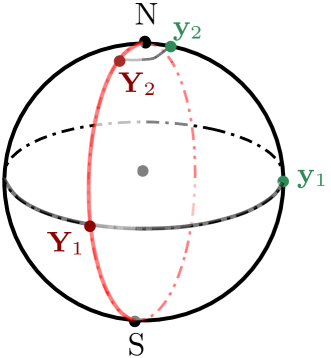
Figure 8: Graphical illustration of geodesic distances between $\bm{y}_{1}$ and $\bm{Y}_{1}$ as well as $\bm{y}_{2}$ and $\bm{Y}_{2}$.

Example 1.

Suppose that we want to estimate the density values at $\bm{y}_{1}=(0,0)$ and $\bm{y}_{2}=(0,\frac{\pi}{2}-\epsilon)$, where $\epsilon>0$ is of a small value. Consider a random sample consisting of only two observations $\bm{Y}_{1}=(\frac{\pi}{2},0)$ and $\bm{Y}_{2}=(\frac{\pi}{2},\frac{\pi}{2}-\epsilon)$. If we use the Euclidean distance, the distance between $(\bm{y}_{1},\bm{Y}_{1})$ and the distance between $(\bm{y}_{2},\bm{Y}_{2})$ are the same. Therefore, when we use the Euclidean KDE $\widehat{p}_{n}$ to estimate the underlying density, the contribution of $\bm{Y}_{1}$ to $\bm{y}_{1}$ will be the same as the contribution of $\bm{Y}_{2}$ to $\bm{y}_{2}$. Nevertheless, their geodesic distances are very different, because $d_{g}(\bm{y}_{1},\bm{Y}_{1})=\frac{\pi}{2}$ while $d_{g}(\bm{y}_{2},\bm{Y}_{2})=\arccos\left[\sin^{2}\left(\frac{\pi}{2}-\epsilon\right)\right]=\arccos\left[\frac{1+\cos(2\epsilon)}{2}\right]$ is a quantity close to zero; see Figure 8 for a graphical illustration. It explains, from a different angle, why the Euclidean KDE $\widehat{p}_{n}$ will have a large bias in estimating the underlying density when the query point $\bm{y}$ is within the high latitude region.

B.2 Case II: Ridge-Finding Problem

Consider the following simulated example of identifying a density ridge via the Euclidean SCMS algorithm (Algorithm 1) and our proposed directional SCMS algorithm (Algorithm 2). We generate 1000 data points $\{\bm{X}_{1},...,\bm{X}_{1000}\}\subset\Omega_{2}$ uniformly frbecauseom a great circle connecting the North and South Poles of $\Omega_{2}$ with some i.i.d. additive Gaussian noises $N(0,0.2^{2})$ to their Cartesian coordinates. Then, all the simulated points will be standardized back to $\Omega_{2}$ via $L_{2}$ normalization. The angular coordinates of these simulated points are denoted by $\{\bm{Y}_{1},...,\bm{Y}_{1000}\}\subset[-180^{\circ},180^{\circ})\times\left[-90^{\circ},90^{\circ}\right]$ accordingly. Figure 9 presents the result of applying both the Euclidean SCMS algorithm (with the Gaussian kernel) to angular coordinates and the directional SCMS algorithm (with the von Mises kernel) to Cartesian coordinates of our simulated dataset. As shown in the panel (b) of Figure 9, the Euclidean SCMS algorithm exhibits high bias in estimating the true circular structure near two poles of $\Omega_{2}$, while our directional SCMS algorithm is able to seek out the true circular structure under negligible errors. The density plot in the panel (c) of Figure 9 exhibits two nonsmoothing peaks on the North Pole due to the infinite Hessian matrices of the underlying density in its angular coordinate; recall our discussion in Section B.1. This also explains the chaotic behavior of the Euclidean KDE in high-latitude regions.

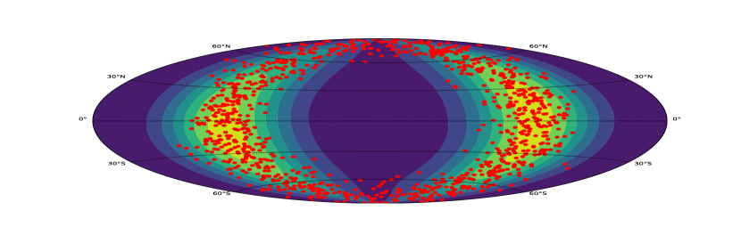
(a) Initial points

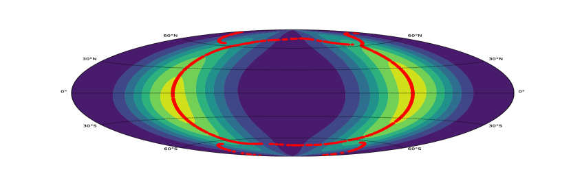
(b) Converged points (hammer projection)

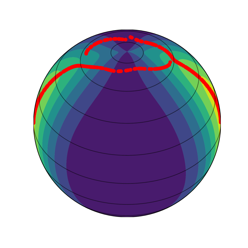
(c) Converged points (orthographic projection)

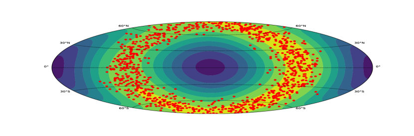
(d) Initial points

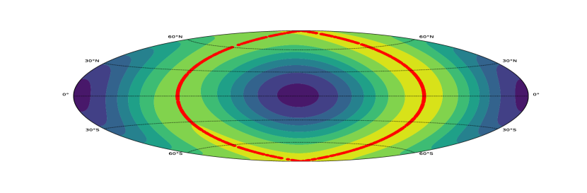
(e) Converged points (hammer projection)

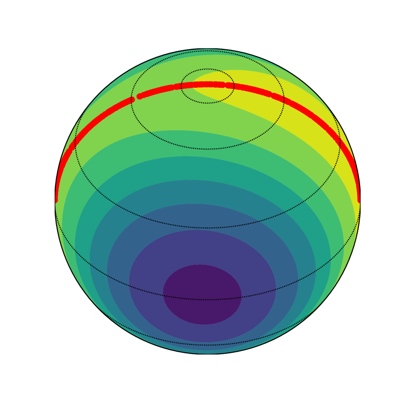
(f) Converged points (orthographic projection)

Figure 9: Euclidean and directional SCMS algorithms performed on the simulated dataset. Panels (a)-(c): Outcomes of the Euclidean SCMS algorithm with the contour plot for the Euclidean KDE. Panels (d)-(f): Outcomes of our directional SCMS algorithm with the contour plot for the directional KDE. Panels (a)-(b) and (d)-(e) are shown in the view of Hammer projections (page 160 in Snyder et al. 1989), while Panels (c) and (f) are presented under the orthographic projections.

At this point, some readers may have a natural concern: why we do not directly apply the Euclidean SCMS algorithm to the Cartesian coordinates $\left\{\bm{X}_{1},...,\bm{X}_{n}\right\}\subset\Omega_{q}$ of the available data points? We discuss the potential downsides of this approach from two different aspects.

1. The Euclidean SCMS algorithm is not intrinsically designed for handling the directional data $\left\{\bm{X}_{1},...,\bm{X}_{n}\right\}\subset\Omega_{q}$. Directly applying the algorithm to these Cartesian coordinates leads to an estimated ridge not lying on $\Omega_{q}$. While the $L_{2}$ normalization is able to standardize the ridge points back to $\Omega_{q}$, this standardization process will inevitable introduce extra bias.

2. When estimating the underlying density of $\left\{\bm{X}_{1},...,\bm{X}_{n}\right\}\subset\Omega_{q}$, we know from (16) and some KDE literature (Chacón et al., 2011; Scott, 2015; Chen, 2017) that the (uniform) rates of convergence of the Euclidean KDE and its derivatives depend on the dimension $(q+1)$ of the ambient space instead of the intrinsic dimension $q$ of directional data. This dimensionality effect also appears in the (linear) convergence of the downstream SCMS algorithm, which, for instance, shrinks the upper bounds of the (linear) convergence radius and step size threshold in Theorem 3.6. Thus, analyzing directional data $\left\{\bm{X}_{1},...,\bm{X}_{n}\right\}\subset\Omega_{q}$ with the Euclidean KDE and SCMS algorithm will slow down the statistical and algorithmic rates of convergence of the density estimators as well as lower the accuracy of the resulting ridge in recovering the underlying structure inside the dataset.

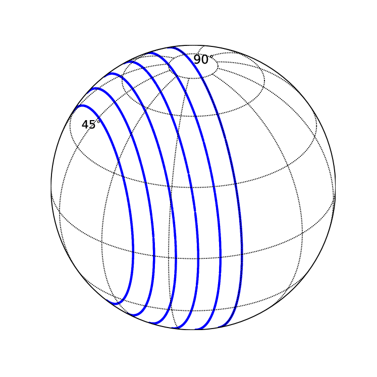
(a) Depiction of underlying true circular structures.

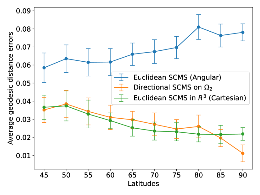
(b) Average geodesic distance errors.

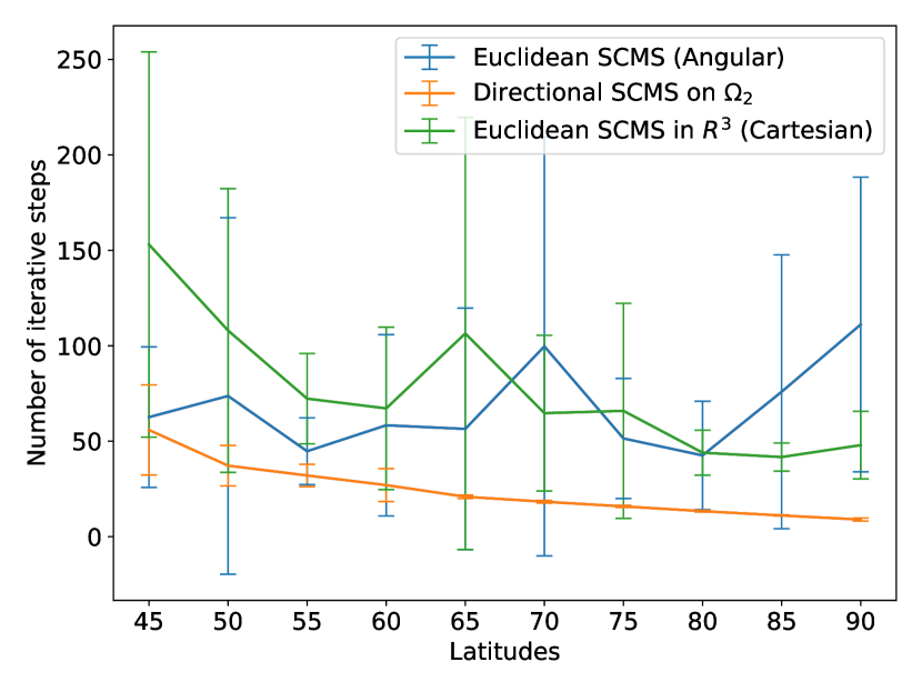
(c) Number of iteration steps.

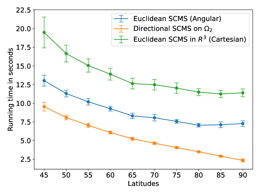
(d) Running time.

Figure 10: Euclidean and directional SCMS algorithms applied to the simulated datasets whose true structures are circles on $\Omega_{2}$ attaining their maximum latitudes from $45^{\circ}$ to $90^{\circ}$, respectively. The dots on each line plot in the panels (b-d) are the means of the associated statistics for the repeated experiments, while the error bars indicate their corresponding standard deviations.

To support our above explanations, we extend our simulation study in Figure 9 as follows. We vary the maximum latitude attained by the underlying (intrinsic) circular structure on $\Omega_{2}$ from $45^{\circ}$ to $90^{\circ}$ while keeping the circle parallel to the original great circle connecting the North and South Poles of $\Omega_{2}$; see the panel (a) in Figure 10 for an illustration. For each of these underlying circles, we follow the same sampling scheme as in Figure 9, i.e., sampling 1000 points uniformly on the circle with some i.i.d. additive Gaussian noises $N(0,0.2^{2})$ to their Cartesian coordinates and $L_{2}$ normalization back to $\Omega_{2}$. The Cartesian coordinates of the simulated points from each circular structure are denoted by $\left\{\bm{X}_{1},...,\bm{X}_{1000}\right\}\subset\Omega_{2}$ while their angular coordinates are represented by $\left\{\bm{Y}_{1},...,\bm{Y}_{1000}\right\}\subset[-180^{\circ},180^{\circ})\times\left[-90^{\circ},90^{\circ}\right]$. Then, we apply our directional SCMS algorithm to $\left\{\bm{X}_{1},...,\bm{X}_{1000}\right\}$ from each of these simulated datasets. Moreover, the Euclidean SCMS algorithm is applied to both the angular coordinates $\left\{\bm{Y}_{1},...,\bm{Y}_{1000}\right\}$ and Cartesian coordinates $\left\{\bm{X}_{1},...,\bm{X}_{1000}\right\}$ from each of these simulated datasets, where we consider $\left\{\bm{X}_{1},...,\bm{X}_{1000}\right\}$ as a dataset in the ambient space $\mathbb{R}^{3}$ in the latter case. Here, the sets of initial points for the Euclidean and directional SCMS algorithms are the simulated datasets themselves. Finally, we compute the average geodesic distance errors on $\Omega_{2}$ from the resulting ridges to the corresponding true circular structures. To reduce the randomness of our simulation studies, we also repeat the above sampling and experimental procedures 20 times for each true circular structure.

We present our comparisons of the Euclidean and directional SCMS algorithms based on three metrics in Figure 10: (i) average geodesic distance errors between the estimated ridges and the true circular structures, (ii) the number of iteration steps, and (iii) the running time. Notice that, as the latitudes of the underlying circular structures increase, the distance errors of (Euclidean) ridges based on the Euclidean SCMS algorithm applied on the angular coordinates $\left\{\bm{Y}_{1},...,\bm{Y}_{1000}\right\}$ rise. Conversely, the distance errors of directional ridges and the ridges based on the Euclidean SCMS algorithm in $\mathbb{R}^{3}$ decreases when the true circular structures climb on $\Omega_{2}$; see the panel (b) of Figure 10. While the performances of our directional SCMS algorithm and the Euclidean SCMS algorithm in $\mathbb{R}^{3}$ are almost indistinguishable in terms of the average geodesic distance errors, our directional SCMS algorithm significantly outperforms the Euclidean SCMS algorithm with regards to time efficiency; see the panels (c-d) of Figure 10. Note that the Euclidean SCMS algorithm exhibits high variance in the number of iteration steps under the repeated experiments, because each simulated dataset may contain some outliers that are far away from the true circular structure on $\Omega_{2}$ and the Euclidean SCMS algorithm requires exceptionally large iterative steps to converge when initialized from these outliers. Our directional SCMS algorithm, however, is stabler in its iterative step due to the fact that it is adaptive to the geometry of $\Omega_{2}$.

Other potential issues of analyzing directional data with Euclidean methods and ignoring the curvature of $\Omega_{2}$ can be found in Chrisman (2017). In summary, it is highly inadequate and inefficient to handle directional data with the Euclidean KDE and SCMS algorithm, which calls for the needs to introduce the directional KDE (5) and propose our well-designed SCMS algorithm for analyzing directional data (Algorithm 2).

Appendix C Normal Space of the Euclidean Density Ridge

As we will refer to conditions (A1-3) frequently in the next two sections, we restate them here:

• (A1) (Differentiability) We assume that $p$ is bounded and at least four times differentiable with bounded partial derivatives up to the fourth order for every $\bm{x}\in\mathbb{R}^{D}$.

• (A2) (Eigengap) We assume that there exist constants $\rho>0$ and $\beta_{0}>0$ such that $\lambda_{d+1}(\bm{y})\leq-\beta_{0}$ and $\lambda_{d}(\bm{y})-\lambda_{d+1}(\bm{y})\geq\beta_{0}$ for any $\bm{y}\in R_{d}\oplus\rho$.

• (A3) (Path Smoothness) Under the same $\rho,\beta_{0}>0$ in (A2), we assume that there exists another constant $\beta_{1}\in(0,\beta_{0})$ such that

  $$D^{\frac{3}{2}}\left|\left|U_{d}^{\perp}(\bm{y})\nabla p(\bm{y})\right|\right|_{2}\left|\left|\nabla^{3}p(\bm{y})\right|\right|_{\max} \leq\frac{\beta_{0}^{2}}{2},$$

  $$d\cdot D^{\frac{3}{2}}\left|\left|\nabla p(\bm{x})\right|\right|_{2}\left|\left|\nabla^{3}p(\bm{x})\right|\right|_{\max} \leq\beta_{0}(\beta_{0}-\beta_{1})$$

  for all $\bm{y}\in R_{d}\oplus\rho$ and $\bm{x}\in R_{d}$.

Given a matrix-valued function $B:\mathbb{R}^{D}\to\mathbb{R}^{m\times n}$, its gradient $\nabla B(\bm{x})$ will be an $m\times n\times D$ array defined as $\left[B(\bm{x})\right]_{ijk}=\frac{\partial}{\partial x_{k}}B(\bm{x})_{ij}$. The derivative of $B$ in the directional of a vector $\bm{z}\in\mathbb{R}^{D}$ is defined as:

$$B^{\prime}(\bm{x};\bm{z})\equiv\lim_{\epsilon\to 0}\frac{B(\bm{x}+\epsilon\bm{z})-B(\bm{x})}{\epsilon}=\nabla B(\bm{x})\bm{z}.$$

When the matrix $A(\bm{x})=\nabla\nabla f(\bm{x})\in\mathbb{R}^{D\times D}$, we will use the notation $\nabla\nabla f^{\prime}(\bm{x};\bm{z})=\nabla^{3}f(\bm{x})\bm{z}\equiv\bm{z}^{T}\nabla^{3}f(\bm{x})$ interchangeably to denote its directional derivative along $\bm{z}$.

Recall that an order-$d$ ridge of the density $p$ in $\mathbb{R}^{D}$ is the collection of points defined as:

$$R_{d}=\left\{\bm{x}\in\mathbb{R}^{D}:G_{d}(\bm{x})=\bm{0},\lambda_{d+1}(\bm{x})<0\right\}=\left\{\bm{x}\in\mathbb{R}^{D}:V_{d}(\bm{x})^{T}\nabla p(\bm{x})=\bm{0},\lambda_{d+1}(\bm{x})<0\right\}.$$

Lemma C.1 below shows that under conditions (A1-3), the Jacobian matrix $\nabla\left[V_{d}(\bm{x})^{T}\nabla p(\bm{x})\right]$ has rank $D-d$ at every point of $R_{d}$, and $R_{d}$ is a $d$-dimensional manifold by the implicit function theorem (Rudin, 1976). Consequently, the row space of $\nabla\left[V_{d}(\bm{x})^{T}\nabla p(\bm{x})\right]\in\mathbb{R}^{(D-d)\times D}$ spans the normal space to $R_{d}$.

If we define $M(\bm{x})=\nabla\left[V_{d}(\bm{x})^{T}\nabla p(\bm{x})\right]^{T}=\left[\bm{m}_{d+1}(\bm{x}),...,\bm{m}_{D}(\bm{x})\right]\in\mathbb{R}^{D\times(D-d)}$, the derivation in pages 60-63 of Eberly (1996) shows that

$$\bm{m}_{k}(\bm{x})=\left[\lambda_{k}(\bm{x})\bm{I}_{D}+\sum_{i=1}^{d}\frac{\bm{v}_{i}(\bm{x})^{T}\nabla p(\bm{x})}{\lambda_{k}(\bm{x})-\lambda_{i}(\bm{x})}\cdot\bm{v}_{i}(\bm{x})^{T}\nabla^{3}p(\bm{x})\right]\bm{v}_{k}(\bm{x})$$ (50)

for $k=d+1,...,D$, and the column space of $M(\bm{x})$ spans the normal space to $R_{d}$. Let

$$\Lambda_{0}(\bm{x}) =\mathtt{Diag}\left[\lambda_{d+1}(\bm{x}),...,\lambda_{D}(\bm{x})\right],$$

$$\Lambda_{i}(\bm{x}) =\mathtt{Diag}\left[\frac{1}{\lambda_{d+1}(\bm{x})-\lambda_{i}(\bm{x})},...,\frac{1}{\lambda_{D}(\bm{x})-\lambda_{i}(\bm{x})}\right],$$

$$T_{i}(\bm{x}) =\left[\bm{v}_{i}(\bm{x})^{T}\nabla p(\bm{x})\right]\cdot\bm{v}_{i}(\bm{x})^{T}\nabla^{3}p(\bm{x})$$

for $i=1,...,d$. Then,

$$M(\bm{x})=V_{d}(\bm{x})\Lambda_{0}(\bm{x})+\sum_{i=1}^{d}T_{i}(\bm{x})V_{d}(\bm{x})\Lambda_{i}(\bm{x}).$$ (51)

However, the columns of $M(\bm{x})$ are not orthonormal. Thus, we leverage the orthonormalization in Chen et al. (2015) to construct $N(\bm{x})$ whose columns are orthonormal and span the same column space as $M(\bm{x})$ in the following steps. Under the condition that $M(\bm{x})=\nabla\left[V_{d}(\bm{x})^{T}\nabla p(\bm{x})\right]^{T}$ has full rank $D-d$ at every point $\bm{x}\in R_{d}$ (see Lemma C.1), $M(\bm{x})^{T}M(\bm{x})$ is positive definite, and we perform the Cholesky decomposition on it, that is,

$$M(\bm{x})^{T}M(\bm{x})=J(\bm{x})J(\bm{x})^{T},$$ (52)

where $J(\bm{x})\in\mathbb{R}^{(D-d)\times(D-d)}$ is a lower triangular matrix whose diagonal elements are positive. We then define

$$N(\bm{x})=M(\bm{x})\left[J(\bm{x})^{T}\right]^{-1}.$$ (53)

Notice that $M(\bm{x}),N(\bm{x}),J(\bm{x})$ intrinsically depend on the dimension $d$ of the ridge $R_{d}$, but we do not explicate these dependencies in their notations. As discussed in Chen et al. (2015), $M(\bm{x})$ might not be unique because the eigenvalues of $\nabla\nabla p(\bm{x})$ can have their multiplicities greater than 1. Any collection of linearly independent unit eigenvectors of $\nabla\nabla p(\bm{x})$ fits into the above construction for $M(\bm{x})$. However, as will be shown later, this volatility of $M(\bm{x})$ will not affect our results, as we only require the smoothness of $M(\bm{x})^{T}M(\bm{x})$ to develop a lower bound of $\mathtt{reach}(R_{d})$.

Lemma C.1.

Assume conditions (A1-3). Given that $M(\bm{x})$ and $N(\bm{x})$ are defined in (51) and (53), we have the following properties:

1. $N(\bm{x})$ and $M(\bm{x})$ have the same column space. In addition,

   $$N(\bm{x})N(\bm{x})^{T}=M(\bm{x})\left[M(\bm{x})^{T}M(\bm{x})\right]^{-1}M(\bm{x})^{T}.$$

   That is, $N(\bm{x})N(\bm{x})^{T}$ is the projection matrix onto the columns of $M(\bm{x})$.

2. The columns of $N(\bm{x})$ are orthonormal to each other.

3. For $\bm{x}\in R_{d}$, the column space of $N(\bm{x})$ is normal to the (tangent) direction of $R_{d}$ at $\bm{x}$.

4. For all $\bm{x}\in R_{d}$, $\mathtt{rank}(N(\bm{x}))=\mathtt{rank}(M(\bm{x}))=D-d$. Moreover, $R_{d}$ is a $d$-dimensional manifold that contains neither intersections and nor endpoints. Namely, $R_{d}$ is a finite union of connected and compact manifolds.

5. For $\bm{x}\in R_{d}$, all the $(D-d)$ nonzero singular values of $M(\bm{x})$ are greater than $\beta_{1}>0$ and therefore,

   $$\left|\left|\left[M(\bm{x})^{T}M(\bm{x})\right]^{-1}\right|\right|_{2}\leq\frac{1}{\beta_{1}^{2}}\quad\text{ and }\quad\left|\left|\left[J(\bm{x})^{T}\right]^{-1}\right|\right|_{2}\leq\frac{1}{\beta_{1}}.$$

6. When $\left|\left|\bm{x}-\bm{y}\right|\right|_{2}$ is sufficiently small and $\bm{x},\bm{y}\in R_{d}\oplus\rho$,

   $$\left|\left|N(\bm{x})N(\bm{x})^{T}-N(\bm{y})N(\bm{y})^{T}\right|\right|_{\max}\leq A_{0}\left(\left|\left|p\right|\right|_{\infty}^{(3)}+\left|\left|p\right|\right|_{\infty}^{(4)}\right)^{2}\left|\left|\bm{x}-\bm{y}\right|\right|_{2}$$

   for some constant $A_{0}>0$.

7. Assume that another density function $q$ also satisfies conditions (A1-3) and $\left|\left|p-q\right|\right|_{\infty,3}^{*}$ is sufficiently small. Then

   $$\left|\left|N_{p}(\bm{x})N_{p}(\bm{x})^{T}-N_{q}(\bm{x})N_{q}(\bm{x})^{T}\right|\right|_{\max}\leq A_{1}\cdot\left|\left|p-q\right|\right|_{\infty,3}^{*}$$

   for some constant $A_{1}>0$ and any $\bm{x}\in R_{d}$, where $N_{p}(\bm{x})$ is the matrix defined in (53) with the underlying density $p$.

8. The reach of $R_{d}$ satisfies

   $$\mathtt{reach}(R_{d})\geq\min\left\{\frac{\rho}{2},\frac{\beta_{1}^{2}}{A_{2}\left(\left|\left|p\right|\right|_{\infty}^{(3)}+\left|\left|p\right|\right|_{\infty}^{(4)}\right)}\right\}$$

   for some constant $A_{2}>0$.

Lemma C.1 is extended from Lemma 2 in Chen et al. (2015) to handle the density ridge $R_{d}$ with $1\leq d<D$. As our conditions (A1-3) imply the imposed conditions of Lemma 2 in Chen et al. (2015), our proof of Lemma C.1 essentially follows from their arguments with some minor modifications.

Proof of Lemma C.1.

We adopt and generalize parts of the proof of Lemma 2 in Chen et al. (2015).
(a) This property is a natural corollary of the Cholesky decomposition as:

$$N(\bm{x})N(\bm{x})^{T}=M(\bm{x})\left[J(\bm{x})^{T}\right]^{-1}J(\bm{x})^{-1}M(\bm{x})^{T}=M(\bm{x})\left[M(\bm{x})^{T}M(\bm{x})\right]^{-1}M(\bm{x})^{T}.$$

(b) Some direct calculations show that

$$N(\bm{x})^{T}N(\bm{x}) =J(\bm{x})^{-1}M(\bm{x})^{T}M(\bm{x})\left[J(\bm{x})^{T}\right]^{-1}$$

$$=J(\bm{x})^{-1}M(\bm{x})^{T}M(\bm{x})\left[J(\bm{x})^{T}\right]^{-1}J(\bm{x})^{-1}J(\bm{x})$$

$$=J(\bm{x})^{-1}M(\bm{x})^{T}M(\bm{x})\left[M(\bm{x})^{T}M(\bm{x})\right]^{-1}J(\bm{x})$$

$$=\bm{I}_{D-d}.$$

(c) It can be proved by the argument of Lemma 1 in Chen et al. (2015). Or, we define an arbitrary parametrized curve $\gamma:(-\epsilon,\epsilon)\to\mathbb{R}^{D}$ lying within $R_{d}$ for some $\epsilon>0$. Then $\gamma^{\prime}(t)$ aligns with the tangent direction at $\gamma(t)\in R_{d}$. Since $V_{d}(\gamma(t))^{T}\nabla p(\gamma(t))=\bm{0}$, taking the derivative with respect to $t$ gives us that

$$0=\frac{d}{dt}\left[V_{d}(\gamma(t))^{T}\nabla p(\gamma(t))\right]=\nabla\left[V_{d}(\bm{x})^{T}\nabla p(\bm{x})\right]\cdot\gamma^{\prime}(t)$$

with $\bm{x}=\gamma(t)$. Hence, by the arbitrariness of $\gamma(t)$, the column of $M(\bm{x})=\nabla\left[V_{d}(\bm{x})^{T}\nabla p(\bm{x})\right]^{T}$ is normal to the tangent direction of $R_{d}$ at $\bm{x}$.

(d) We prove that the $(D-d)$ nonzero singular values of $M(\bm{x})\in\mathbb{R}^{D\times(D-d)}$ are bounded away from 0. Recall that

$$M(\bm{x})=V_{d}(\bm{x})\Lambda_{0}(\bm{x})+\sum_{i=1}^{d}T_{i}(\bm{x})V_{d}(\bm{x})\Lambda_{i}(\bm{x})$$

with

$$\Lambda_{0}(\bm{x}) =\mathtt{Diag}\left[\lambda_{d+1}(\bm{x}),...,\lambda_{D}(\bm{x})\right],$$

$$\Lambda_{i}(\bm{x}) =\mathtt{Diag}\left[\frac{1}{\lambda_{d+1}(\bm{x})-\lambda_{i}(\bm{x})},...,\frac{1}{\lambda_{D}(\bm{x})-\lambda_{i}(\bm{x})}\right],$$

$$T_{i}(\bm{x}) =\left[\bm{v}_{i}(\bm{x})^{T}\nabla p(\bm{x})\right]\cdot\bm{v}_{i}(\bm{x})^{T}\nabla^{3}p(\bm{x})$$

for $i=1,...,d$. Under conditions (A2-3),

$$\left|\left|\sum_{i=1}^{d}T_{i}(\bm{x})V_{d}(\bm{x})\Lambda_{i}(\bm{x})\right|\right|_{2}$$

$$\leq\sum_{i=1}^{d}\left|\left|T_{i}(\bm{x})\right|\right|_{2}\cdot\left|\left|V_{d}(\bm{x})\right|\right|_{2}\cdot\frac{1}{\beta_{0}}\quad\text{ by condition (A2)}$$

$$\leq\sum_{i=1}^{d}\left|\left|\left[\bm{v}_{i}(\bm{x})^{T}\nabla p(\bm{x})\right]\cdot\bm{v}_{i}(\bm{x})^{T}\nabla^{3}p(\bm{x})\right|\right|_{2}\cdot\frac{1}{\beta_{0}}\quad\text{ since }\left|\left|V_{d}(\bm{x})\right|\right|_{2}=1$$

$$\leq\frac{d\left|\left|\nabla p(\bm{x})\right|\right|_{2}\cdot D^{\frac{3}{2}}\left|\left|\nabla^{3}p(\bm{x})\right|\right|_{\max}}{\beta_{0}}$$

$$\leq\beta_{0}-\beta_{1}\quad\text{ by condition (A3)}.$$

It shows that all the singular values of $\sum\limits_{i=1}^{d}T_{i}(\bm{x})V_{d}(\bm{x})\Lambda_{i}(\bm{x})$ are less than $\beta_{0}-\beta_{1}$. Moreover, under condition (A2) again, all the $(D-d)$ nonzero singular values of $V_{d}(\bm{x})\Lambda_{0}(\bm{x})$ are greater than $\beta_{0}$. By Theorem 3.3.16 in Horn and Johnson (1991), we know that all the $(D-d)$ nonzero singular values of $M(\bm{x})$ are greater than $\beta_{0}-(\beta_{0}-\beta_{1})=\beta_{1}>0$. Therefore, $\mathtt{rank}(M(\bm{x}))=\mathtt{rank}(N(\bm{x}))=D-d$. The rest of the proof follows directly from Claim 4 in Chen et al. (2015).

(e) By the proof of (d), we already know that all the $(D-d)$ nonzero singular values of $M(\bm{x})$ are greater than $\beta_{1}>0$. Thus, $\left|\left|\left[M(\bm{x})^{T}M(\bm{x})\right]^{-1}\right|\right|_{2}\leq\frac{1}{\beta_{1}^{2}}$, and

$$\left|\left|\left[J(\bm{x})^{T}\right]^{-1}\right|\right|_{2}=\sqrt{\frac{1}{\sigma_{\min}\left(J(\bm{x})J(\bm{x})^{T}\right)}} =\sqrt{\frac{1}{\sigma_{\min}\left(M(\bm{x})^{T}M(\bm{x})\right)}}$$

$$=\sqrt{\left|\left|\left[M(\bm{x})^{T}M(\bm{x})\right]^{-1}\right|\right|_{2}}\leq\frac{1}{\beta_{1}},$$

where $\sigma_{\min}(A)$ is the smallest singular value of matrix $A$.

Finally, the proofs of properties (f), (g), and (h) are essentially the same as the corresponding claims in Chen et al. (2015). We thus omitted them. ∎

As we have discussed in Remark 4.1, property (d) of Lemma C.1 demonstrates that our imposed assumptions (A1-3) for the ridge $R_{d}$ is sufficient to imply the critical full-rank condition of its normal space in Chen (2020) in order for $R_{d}$ to be a well-defined solution manifold.

Appendix D Proofs of Lemma 3.2, Proposition 3.3, and Theorem 3.6

Lemma 3.2.

Assume conditions (A1) and (E1). The convergence rate of $\widehat{g}_{n}(\bm{x})=\frac{2c_{k,D}}{nh^{D+2}}\sum\limits_{i=1}^{n}-k^{\prime}\left(\left|\left|\frac{\bm{x}-\bm{X}_{i}}{h}\right|\right|_{2}^{2}\right)$ is

$$h^{2}\widehat{g}_{n}(\bm{x}) =-2c_{k,D}\cdot p(\bm{x})\int_{\mathbb{R}^{D}}k^{\prime}\left(\left|\left|\bm{u}\right|\right|_{2}^{2}\right)d\bm{u}+O\left(h^{2}\right)+O_{P}\left(\sqrt{\frac{1}{nh^{D}}}\right)$$

$$=O(1)+O\left(h^{2}\right)+O_{P}\left(\sqrt{\frac{1}{nh^{D}}}\right)$$

for any $\bm{x}\in\mathbb{R}^{D}$ as $nh^{D}\to\infty$ and $h\to 0$.

Another interpretation of Lemma 3.2 is that $\widehat{g}_{n}(\bm{x})$ diverges to infinity at the rate

$$O\left(h^{-2}\right)+O_{P}\left(\sqrt{\frac{1}{nh^{D+4}}}\right)=O\left(n^{\frac{2}{D+4}}\right)+O_{P}\left(1\right)$$

if we select the bandwidth $h_{\text{opt}}\asymp O\left(n^{-\frac{1}{D+4}}\right)$ to minimize the asymptotic mean integrated square error (Chen, 2017), where “$\asymp$” stands for the asymptotic equivalence.

Proof of Lemma 3.2.

Note that

$$h^{2}\widehat{g}_{n}(\bm{x})=\mathbb{E}\left[h^{2}\widehat{g}_{n}(\bm{x})\right]+h^{2}\widehat{g}_{n}(\bm{x})-\mathbb{E}\left[h^{2}\widehat{g}_{n}(\bm{x})\right].$$ (54)

Given the differentiability of $p$ guaranteed by condition (A1), the expectation of $h^{2}\widehat{g}_{n}(\bm{x})$ is given by:

$$\mathbb{E}\left[h^{2}\widehat{g}_{n}(\bm{x})\right] =\frac{2c_{k,D}}{h^{D}}\int_{\mathbb{R}^{D}}-k^{\prime}\left(\left|\left|\frac{\bm{x}-\bm{y}}{h}\right|\right|_{2}^{2}\right)\cdot p(\bm{y})d\bm{y}$$

$$=2c_{k,D}\int_{\mathbb{R}^{D}}-k^{\prime}\left(\left|\left|\bm{u}\right|\right|_{2}^{2}\right)\cdot p(\bm{x}+h\bm{u})d\bm{u}\quad\text{ by }\bm{u}=\frac{\bm{y}-\bm{x}}{h}$$

$$=2c_{k,D}\int_{\mathbb{R}^{D}}-k^{\prime}\left(\left|\left|\bm{u}\right|\right|_{2}^{2}\right)\left[p(\bm{x})+h\nabla p(\bm{x})^{T}\bm{u}+O(h^{2})\right]d\bm{u}$$

$$=2c_{k,D}\cdot p(\bm{x})\int_{\mathbb{R}^{D}}-k^{\prime}\left(\left|\left|\bm{u}\right|\right|_{2}^{2}\right)d\bm{u}+O(h^{2}).$$

By condition (E1), the dominating constant $-2c_{k,D}\cdot p(\bm{x})\int_{\mathbb{R}^{D}}k^{\prime}\left(\left|\left|\bm{u}\right|\right|_{2}^{2}\right)d\bm{u}$ is finite and therefore,

$$\mathbb{E}\left[h^{2}\widehat{g}_{n}(\bm{x})\right]=-2c_{k,D}\cdot p(\bm{x})\int_{\mathbb{R}^{D}}k^{\prime}\left(\left|\left|\bm{u}\right|\right|_{2}^{2}\right)d\bm{u}+O\left(h^{2}\right)=O(1)+O(h^{2}).$$ (55)

In addition, we calculate the variance of $\widehat{g}_{n}(\bm{x})$ as

$$\text{Var}\left[h^{2}\widehat{g}_{n}(\bm{x})\right]$$

$$=\frac{4c_{k,D}^{2}}{nh^{2D}}\cdot\text{Var}\left[k^{\prime}\left(\left|\left|\frac{\bm{x}-\bm{X}_{1}}{h}\right|\right|_{2}^{2}\right)\right]$$

$$=\frac{4c_{k,D}^{2}}{nh^{2D}}\int_{\mathbb{R}^{D}}k^{\prime}\left(\left|\left|\frac{\bm{x}-\bm{y}}{h}\right|\right|_{2}^{2}\right)^{2}p(\bm{y})\,d\bm{y}-\frac{1}{n}\left\{\mathbb{E}\left[h^{2}\widehat{g}_{n}(\bm{x})\right]\right\}^{2}$$

$$=\frac{4c_{k,D}^{2}}{nh^{D}}\int_{\mathbb{R}^{D}}k^{\prime}\left(\left|\left|\bm{u}\right|\right|_{2}^{2}\right)^{2}\cdot p(\bm{x}+h\bm{u})d\bm{u}-\frac{1}{n}\left[O(1)+O\left(h^{2}\right)\right]^{2}\quad\text{ by }\bm{u}=\frac{\bm{y}-\bm{x}}{h}$$

$$=\frac{4c_{k,D}^{2}}{nh^{D}}\int_{\mathbb{R}^{D}}k^{\prime}\left(\left|\left|\bm{u}\right|\right|_{2}^{2}\right)^{2}\left[p(\bm{x})+h\nabla p(\bm{x})^{T}\bm{u}+O(h^{2})\right]d\bm{u}+o\left(\frac{1}{nh^{D}}\right)$$

$$=\frac{4c_{k,D}^{2}\cdot p(\bm{x})}{nh^{D}}\int_{\mathbb{R}^{D}}k^{\prime}\left(\left|\left|\bm{u}\right|\right|_{2}^{2}\right)^{2}d\bm{u}+o\left(\frac{1}{nh^{D}}\right),$$

Again, by condition (E1), the dominating constant $4c_{k,D}^{2}\cdot p(\bm{x})\int_{\mathbb{R}^{D}}k^{\prime}\left(\left|\left|\bm{u}\right|\right|_{2}^{2}\right)^{2}d\bm{u}$ is finite. Thus, by the central limit theorem,

$$\begin{split}h^{2}\widehat{g}_{n}(\bm{x})-\mathbb{E}\left[h^{2}\widehat{g}_{n}(\bm{x})\right]&=\sqrt{\text{Var}\left[h^{2}\widehat{g}_{n}(\bm{x})\right]}\cdot\frac{h^{2}\widehat{g}_{n}(\bm{x})-\mathbb{E}\left[h^{2}\widehat{g}_{n}(\bm{x})\right]}{\sqrt{\text{Var}\left[h^{2}\widehat{g}_{n}(\bm{x})\right]}}\\ &=\sqrt{\text{Var}\left[h^{2}\widehat{g}_{n}(\bm{x})\right]}\cdot\bm{Z}_{n}(\bm{x})\\ &=O_{P}\left(\sqrt{\frac{1}{nh^{D}}}\right),\end{split}$$ (56)

where $\bm{Z}_{n}(\bm{x})\stackrel{{\scriptstyle d}}{{\to}}\mathcal{N}_{D}(\bm{0},\bm{I}_{D})$. Combining (54), (55), and (56), we conclude that

$$h^{2}\widehat{g}_{n}(\bm{x}) =-2c_{k,D}\cdot p(\bm{x})\int_{\mathbb{R}^{D}}k^{\prime}\left(\left|\left|\bm{u}\right|\right|_{2}^{2}\right)+O\left(h^{2}\right)+O_{P}\left(\sqrt{\frac{1}{nh^{D}}}\right)$$

$$=O(1)+O\left(h^{2}\right)+O_{P}\left(\sqrt{\frac{1}{nh^{D}}}\right)$$

for any $\bm{x}\in\mathbb{R}^{D}$ as $nh^{D}\to\infty$ and $h\to 0$. ∎

Remark D.1.

Some previous research papers on the mean shift algorithm Li et al. (2007); Carreira-Perpiñán (2007); Aliyari Ghassabeh (2015); Arias-Castro et al. (2016) have already justified that the algorithm converges to a local mode of the KDE $\widehat{p}_{n}$ when its local modes are isolated and the algorithm starts within some small neighborhoods of these estimated local modes. Lemma 3.2 here provides a (probabilistic) perspective on the linear convergence of the mean shift algorithm. It is well-known that the set of the true local modes of $p$ can be approximated by the set of estimated modes defined by $\widehat{p}_{n}$ (Chen et al., 2016). Moreover, around the true local modes of the density $p$, one can argue that $\widehat{p}_{n}$ is strongly convex and has a Lipschitz gradient with probability tending to 1 by the uniform consistency of $\nabla\widehat{p}_{n}$ and $\nabla\nabla\widehat{p}_{n}$ as $h\to 0$ and $\frac{nh^{D+4}}{|\log h|}\to\infty$; see the uniform bounds (16). Hence, by some standard results in optimization theory (e.g., Chapter 3 in Bubeck (2015)), a sample-based gradient ascent algorithm with objective function $\widehat{p}_{n}$ converges linearly to (estimated) local modes around their neighborhoods as long as its step size is below some threshold value. Finally, recall that (i) the mean shift algorithm is a special variant of the sample-based gradient ascent method with an adaptive size $\eta_{n,h}^{(t)}$ by (19) and (ii) $\eta_{n,h}^{(t)}$ can be sufficiently small but bounded away from 0 when $nh^{D}$ is large and $h$ is small by Lemma 3.2; see also Remark 3.2. Therefore, the mean shift algorithm will converge linearly with high probability around some small neighborhood of the local modes of $\widehat{p}_{n}$ when the sample size $n$ is sufficiently large and $h$ is chosen to be small.

Proposition 3.3 (Convergence of the SCGA Algorithm).

For any SCGA sequence $\big{\{}\bm{x}^{(t)}\big{\}}_{t=0}^{\infty}$ defined by (23) with $0<\eta<\frac{2}{D\left|\left|p\right|\right|_{\infty}^{(2)}}$, the following properties hold.

1. Under condition (A1), the objective function sequence $\big{\{}p(\bm{x}^{(t)})\big{\}}_{t=0}^{\infty}$ is non-decreasing and converges.

2. Under condition (A1), $\lim_{t\to\infty}\left|\left|V_{d}(\bm{x}^{(t)})^{T}\nabla p(\bm{x}^{(t)})\right|\right|_{2}=\lim_{t\to\infty}\left|\left|\bm{x}^{(t+1)}-\bm{x}^{(t)}\right|\right|_{2}=0$.

3. Under conditions (A1-3), $\lim_{t\to\infty}d_{E}(\bm{x}^{(t)},R_{d})=0$ whenever $\bm{x}^{(0)}\in R_{d}\oplus r_{1}$ with the convergence radius $r_{1}$ satisfying

   $$0<r_{1}<\min\left\{\frac{\rho}{2},\;\frac{\beta_{1}^{2}}{A_{2}\left(\left|\left|p\right|\right|_{\infty}^{(3)}+\left|\left|p\right|\right|_{\infty}^{(4)}\right)},\;\frac{\beta_{1}}{A_{4}(p)}\right\},$$

   where $A_{2}>0$ is a constant defined in (h) of Lemma C.1 while $A_{4}(p)>0$ is a quantity depending on both the dimension $D$ and functional norm $\left|\left|p\right|\right|_{\infty,4}^{*}$ up to the fourth-order (partial) derivatives of $p$.

Proof of Proposition 3.3.

(a) We first derive the following fact about the objective function $p$.

$\bullet$ Fact 1. Given (A1), $p$ is $D\left|\left|p\right|\right|_{\infty}^{(2)}$-smooth, that is, $\nabla p$ is $D\left|\left|p\right|\right|_{\infty}^{(2)}$-Lipschitz.

This fact follows from the differentiability of $p$ ensured by condition (A1) and Taylor’s theorem that

$$\left|\left|\nabla p(\bm{x})-\nabla p(\bm{y})\right|\right|_{2} \leq\left|\left|\nabla\nabla p(\widetilde{\bm{y}})\right|\right|_{2}\cdot\left|\left|\bm{x}-\bm{y}\right|\right|_{2}\leq D\left|\left|p\right|\right|_{\infty}^{(2)}\cdot\left|\left|\bm{x}-\bm{y}\right|\right|_{2}$$

for any $\bm{x},\bm{y}\in\mathbb{R}^{D}$, where $\widetilde{\bm{y}}$ is within a $\left|\left|\bm{x}-\bm{y}\right|\right|_{2}$-neighborhood of $\bm{y}$. Moreover,

$$\begin{split}\left|p(\bm{y})-p(\bm{x})-\nabla p(\bm{x})^{T}(\bm{y}-\bm{x})\right|&=\int_{0}^{1}\nabla p(\bm{x}+t(\bm{y}-\bm{x}))^{T}(\bm{y}-\bm{x})dt-\nabla p(\bm{x})^{T}(\bm{y}-\bm{x})\\ &\leq\int_{0}^{1}\left|\left|\nabla p(\bm{x}+t(\bm{y}-\bm{x}))-p(\bm{x})\right|\right|_{2}\cdot\left|\left|\bm{y}-\bm{x}\right|\right|_{2}dt\\ &\leq\frac{D\left|\left|p\right|\right|_{\infty}^{(2)}}{2}\cdot\left|\left|\bm{y}-\bm{x}\right|\right|_{2}^{2}.\end{split}$$ (57)

When $0<\eta<\frac{2}{D\left|\left|p\right|\right|_{\infty}^{(2)}}$, we have that

$$\begin{split}&p(\bm{x}^{(t+1)})-p(\bm{x}^{(t)})\\ &=p\left(\bm{x}^{(t)}+\eta\cdot V_{d}(\bm{x}^{(t)})V_{d}(\bm{x}^{(t)})^{T}\nabla p(\bm{x}^{(t)})\right)-p(\bm{x}^{(t)})\\ &\geq\nabla p(\bm{x}^{(t)})^{T}\cdot\eta V_{d}(\bm{x}^{(t)})V_{d}(\bm{x}^{(t)})^{T}\nabla p(\bm{x}^{(t)})-\frac{D\left|\left|p\right|\right|_{\infty}^{(2)}}{2}\eta^{2}\left|\left|V_{d}(\bm{x}^{(t)})^{T}\nabla p(\bm{x}^{(t)})\right|\right|_{2}^{2}\quad\text{ by \eqref{L_smoothness}}\\ &=\eta\left(1-\frac{D\left|\left|p\right|\right|_{\infty}^{(2)}\eta}{2}\right)\left|\left|V_{d}(\bm{x}^{(t)})^{T}\nabla p(\bm{x}^{(t)})\right|\right|_{2}^{2}\geq 0,\end{split}$$ (58)

showing that the objective function $p$ is non-decreasing along $\big{\{}\bm{x}^{(t)}\big{\}}_{t=0}^{\infty}$. Given the boundedness of $p$ guaranteed by condition (A1), we know that the sequence $\left\{p(\bm{x}^{(t)})\right\}_{t=0}^{\infty}$ is bounded. Thus, $\left\{p(\bm{x}^{(t)})\right\}_{t=0}^{\infty}$ also converges.

(b) From (a), we know that when $0<\eta<\frac{2}{D\left|\left|p\right|\right|_{\infty}^{(2)}}$,

$$p(\bm{x}^{(t+1)})-p(\bm{x}^{(t)}) \geq\eta\left(1-\frac{D\left|\left|p\right|\right|_{\infty}^{(2)}\eta}{2}\right)\left|\left|V_{d}(\bm{x}^{(t)})^{T}\nabla p(\bm{x}^{(t)})\right|\right|_{2}^{2}$$

$$=\left(\frac{2-D\left|\left|p\right|\right|_{\infty}^{(2)}\eta}{2\eta}\right)\left|\left|\bm{x}^{(t+1)}-\bm{x}^{(t)}\right|\right|_{2}^{2}.$$

Since the sequence $\left\{p(\bm{x}^{(t)})\right\}_{t=0}^{\infty}$ converges as $t\to\infty$, it follows that

$$\lim_{t\to\infty}\left|\left|V_{d}(\bm{x}^{(t)})^{T}\nabla p(\bm{x}^{(t)})\right|\right|_{2}=0\quad\text{ and }\quad\lim_{t\to\infty}\left|\left|\bm{x}^{(t+1)}-\bm{x}^{(t)}\right|\right|_{2}=0.$$

(c) Given condition (A2) and the fact that $r_{1}<\frac{\rho}{2}$, we know that

$$\bm{x}\in R_{d}\oplus r_{1}\text{ and }\left|\left|V_{d}(\bm{x})^{T}\nabla p(\bm{x})\right|\right|_{2}=0\quad\text{ if and only if}\quad\bm{x}\in R_{d}.$$

Let $\bm{z}^{(t)}=\pi_{R_{d}}(\bm{x}^{(t)})$ denote the projection of $\bm{x}^{(t)}$ in the SCGA sequence onto the ridge $R_{d}$. Since $r_{1}\leq\mathtt{reach}(R_{d})$ by (h) of Lemma C.1, $\bm{z}^{(t)}$ is well-defined when $\bm{x}^{(t)}\in R_{d}\oplus r_{1}$. Given that the definition of $M(\bm{z}^{(t)})=\nabla\left[V_{d}(\bm{z}^{(t)})^{T}\nabla p(\bm{z}^{(t)})\right]^{T}\in\mathbb{R}^{D\times(D-d)}$ in (51), we know that

$$\begin{split}&\left|\left|V_{d}(\bm{x}^{(t)})^{T}\nabla p(\bm{x}^{(t)})\right|\right|_{2}\\ &=\left|\left|V_{d}(\bm{x}^{(t)})^{T}\nabla p(\bm{x}^{(t)})-\underbrace{V_{d}(\bm{z}^{(t)})^{T}\nabla p(\bm{z}^{(t)})}_{=0}\right|\right|_{2}\\ &=\left|\left|\int_{0}^{1}M\left(\bm{z}^{(t)}+\epsilon(\bm{x}^{(t)}-\bm{z}^{(t)})\right)^{T}(\bm{x}^{(t)}-\bm{z}^{(t)})\,d\epsilon\right|\right|_{2}\quad\text{ by Taylor's theorem}\\ &=\left|\left|M(\bm{z}^{(t)})^{T}(\bm{x}^{(t)}-\bm{z}^{(t)})+\int_{0}^{1}\left[M\left(\bm{z}^{(t)}+\epsilon(\bm{x}^{(t)}-\bm{z}^{(t)})\right)-M(\bm{z}^{(t)})\right]^{T}(\bm{x}^{(t)}-\bm{z}^{(t)})\,d\epsilon\right|\right|_{2}\\ &\geq\left|\left|M(\bm{z}^{(t)})^{T}(\bm{x}^{(t)}-\bm{z}^{(t)})\right|\right|_{2}-\frac{1}{2}\sup_{\epsilon\in[0,1]}\left|\left|\nabla M\left(\bm{z}^{(t)}+\epsilon(\bm{x}^{(t)}-\bm{z}^{(t)})\right)^{T}\right|\right|_{2}\left|\left|\bm{x}^{(t)}-\bm{z}^{(t)}\right|\right|_{2}^{2}\\ &\stackrel{{\scriptstyle\text{(i)}}}{{\geq}}\beta_{1}\left|\left|\bm{x}^{(t)}-\bm{z}^{(t)}\right|\right|_{2}-\frac{A_{4}(p)}{2}\left|\left|\bm{x}^{(t)}-\bm{z}^{(t)}\right|\right|_{2}^{2}\\ &=d_{E}(\bm{x}^{(t)},R_{d})\cdot\left(\beta_{1}-\frac{A_{4}(p)}{2}d_{E}(\bm{x}^{(t)},R_{d})\right)\\ &\geq\frac{\beta_{1}}{2}\cdot d_{E}(\bm{x}^{(t)},R_{d})\end{split}$$ (59)

when $\bm{x}^{(t)}\in R_{d}\oplus r_{1}$, where we leverage (e) of Lemma C.1 to obtain the inequality (i). More specifically, $M(\bm{z}^{(t)})^{T}$ is a full row rank matrix by (d) of Lemma C.1 and $\bm{x}^{(t)}-\bm{z}^{(t)}$ lies within the row space of $M(\bm{z}^{(t)})^{T}$ because $\bm{x}^{(t)}-\bm{z}^{(t)}$ is normal to $R_{d}$ at $\bm{z}^{(t)}$. Since the nonzero singular values of $M(\bm{z}^{(t)})$ are lower bounded by $\beta_{1}>0$, it follows that $\left|\left|M(\bm{z}^{(t)})^{T}(\bm{x}^{(t)}-\bm{z}^{(t)})\right|\right|_{2}\geq\beta_{1}\left|\left|\bm{x}^{(t)}-\bm{z}^{(t)}\right|\right|_{2}$. From the above derivation, we also know that $A_{4}(p)>0$ is indeed the supremum norm of $\nabla M(\bm{x})^{T}=\nabla\nabla\left[V_{d}(\bm{x})^{T}\nabla p(\bm{x})\right]^{T}$ over the line segment connecting $\bm{x}^{(t)}$ and $\bm{z}^{(t)}$, which depends on the uniform functional norm $\left|\left|p\right|\right|_{\infty,4}^{*}$ of the partial derivatives of $p$ up to the fourth order. The result follows from (b). ∎

The following Davis-Kahan theorem (Davis and Kahan, 1970) is one of the most notable theorems in matrix perturbation theory. We present the theorem in a modified version from von Luxburg (2007); Genovese et al. (2014). Other useful variants of the Davis-Kahan theorem can be found in Yu et al. (2014).

Lemma D.1 (Davis-Kahan).

Let $H$ and $\widetilde{H}$ be two symmetric matrices in $\mathbb{R}^{D\times D}$, whose spectra (Definition 1.1.4 in Horn and Johnson 2012) are $\sigma(H)$ and $\sigma(\widetilde{H})$, and $S_{1}\subset\mathbb{R}$ be an interval. Denote by $\sigma_{S_{1}}(H)$ the set of eigenvalues of $H$ that are contained in $S_{1}$, and by $V_{1}$ the matrix whose columns are the corresponding (unit) eigenvectors to $\sigma_{S_{1}}(H)$ (more formally, $V_{1}$ is the image of the spectral projection induced by $\sigma_{S_{1}}(H)$). Denote by $\sigma_{S_{1}}(\widetilde{H})$ and $\widetilde{V}_{1}$ the analogous quantities for $\widetilde{H}$. If

$$\delta:=\inf\left\{|\lambda-\widetilde{\lambda}|:\lambda\in\sigma_{S_{1}}(H),\widetilde{\lambda}\in\sigma(\widetilde{H})\setminus\sigma_{S_{1}}(\widetilde{H})\right\}>0,$$

then the distance $d(V_{1},\widetilde{V}_{1}):=\left|\left|\sin\bm{\Theta}(V_{1},\widetilde{V}_{1})\right|\right|$ between two subspaces is bounded by

$$d(V_{1},\widetilde{V}_{1})\leq\frac{\left|\left|H-\widetilde{H}\right|\right|}{\delta}$$

for any orthogonally invariant norm $\left|\left|\cdot\right|\right|$, such as the Frobenius norm $\left|\left|\cdot\right|\right|_{F}$ and the $L_{2}$-operator norm $\left|\left|\cdot\right|\right|_{2}$, where $\bm{\Theta}(V_{1},\widetilde{V}_{1})$ is a diagonal matrix with the ascending principal angles between the column spaces of $V_{1}$ and $\widetilde{V}_{1}$ on the diagonal.

Note that when we take the Frobenius norm in Lemma D.1, $\left|\left|\sin\bm{\Theta}(V_{1},\widetilde{V}_{1})\right|\right|_{F}=\frac{\left|\left|V_{1}V_{1}^{T}-\widetilde{V}_{1}\widetilde{V}_{1}^{T}\right|\right|_{F}}{\sqrt{2}}$ by some simple algebra. Consequently, we will utilize the following inequality from the Davis-Kahan theorem in our subsequent proofs as:

$$\begin{split}\left|\left|V_{1}V_{1}^{T}-\widetilde{V}_{1}\widetilde{V}_{1}^{T}\right|\right|_{2}\leq\left|\left|V_{1}V_{1}^{T}-\widetilde{V}_{1}\widetilde{V}_{1}^{T}\right|\right|_{F}=\sqrt{2}\left|\left|\sin\bm{\Theta}(V_{1},\widetilde{V}_{1})\right|\right|_{F}&\leq\frac{\sqrt{2}\left|\left|H-\widetilde{H}\right|\right|_{F}}{\delta}\\ &\leq\frac{\sqrt{2}D\left|\left|H-\widetilde{H}\right|\right|_{\max}}{\delta}\\ &\leq\frac{\sqrt{2}D\left|\left|H-\widetilde{H}\right|\right|_{2}}{\delta}.\end{split}$$ (60)

Theorem 3.6 (Linear Convergence of the SCGA Algorithm).

Assume conditions (A1-4) throughout the theorem.

1. Q-Linear convergence of $\left|\left|\bm{x}^{(t)}-\bm{x}^{*}\right|\right|_{2}$: Consider a convergence radius $r_{2}>0$ satisfying

   $$0<r_{2}<\min\left\{\frac{\rho}{2},\frac{\beta_{1}^{2}}{A_{2}\left(\left|\left|p\right|\right|_{\infty}^{(3)}+\left|\left|p\right|\right|_{\infty}^{(4)}\right)},\frac{\beta_{1}}{A_{4}(p)},\frac{3\beta_{0}}{4D\left(6\left|\left|p\right|\right|_{\infty}^{(2)}\beta_{2}^{2}\rho+D^{\frac{1}{2}}\left|\left|p\right|\right|_{\infty}^{(3)}\right)}\right\},$$

   where $A_{2}>0$ is the constant defined in (h) of Lemma C.1 and $A_{4}(p)>0$ is a quantity defined in (c) of Proposition 3.3 that depends on both the dimension $D$ and the functional norm $\left|\left|p\right|\right|_{\infty,4}^{*}$ up to the fourth-order derivative of $p$. Whenever $0<\eta\leq\min\left\{\frac{4}{\beta_{0}},\frac{1}{D\left|\left|p\right|\right|_{\infty}^{(2)}}\right\}$ and the initial point $\bm{x}^{(0)}\in\text{Ball}_{D}(\bm{x}^{*},r_{2})$ with $\bm{x}^{*}\in R_{d}$, we have that

   $$\left|\left|\bm{x}^{(t)}-\bm{x}^{*}\right|\right|_{2}\leq\Upsilon^{t}\left|\left|\bm{x}^{(0)}-\bm{x}^{*}\right|\right|_{2}\quad\text{ with }\quad\Upsilon=\sqrt{1-\frac{\beta_{0}\eta}{4}}.$$

2. R-Linear convergence of $d_{E}(\bm{x}^{(t)},R_{d})$: Under the same radius $r_{2}>0$ in (a), we have that whenever $0<\eta\leq\min\left\{\frac{4}{\beta_{0}},\frac{1}{D\left|\left|p\right|\right|_{\infty}^{(2)}}\right\}$ and the initial point $\bm{x}^{(0)}\in\text{Ball}_{D}(\bm{x}^{*},r_{2})$ with $\bm{x}^{*}\in R_{d}$,

   $$d_{E}(\bm{x}^{(t)},R_{d})\leq\Upsilon^{t}\left|\left|\bm{x}^{(0)}-\bm{x}^{*}\right|\right|_{2}\quad\text{ with }\quad\Upsilon=\sqrt{1-\frac{\beta_{0}\eta}{4}}.$$

We further assume conditions (E1-2) in the rest of statements. If $h\to 0$ and $\frac{nh^{D+4}}{|\log h|}\to\infty$,

1. Q-Linear convergence of $\left|\left|\widehat{\bm{x}}^{(t)}-\bm{x}^{*}\right|\right|_{2}$: under the same radius $r_{2}>0$ and $\Upsilon=\sqrt{1-\frac{\beta_{0}\eta}{4}}$ in (a), we have that

   $$\left|\left|\widehat{\bm{x}}^{(t)}-\bm{x}^{*}\right|\right|_{2}\leq\Upsilon^{t}\left|\left|\widehat{\bm{x}}^{(0)}-\bm{x}^{*}\right|\right|_{2}+O(h^{2})+O_{P}\left(\sqrt{\frac{|\log h|}{nh^{D+4}}}\right)$$

   with probability tending to 1 whenever $0<\eta\leq\min\left\{\frac{4}{\beta_{0}},\frac{1}{D\left|\left|p\right|\right|_{\infty}^{(2)}}\right\}$ and the initial point $\widehat{\bm{x}}^{(0)}\in\text{Ball}_{D}(\bm{x}^{*},r_{2})$ with $\bm{x}^{*}\in R_{d}$.

1. R-Linear convergence of $d_{E}(\widehat{\bm{x}}^{(t)},R_{d})$: under the same radius $r_{2}>0$ and $\Upsilon=\sqrt{1-\frac{\beta_{0}\eta}{4}}$ in (a), we have that

   $$d_{E}(\widehat{\bm{x}}^{(t)},R_{d})\leq\Upsilon^{t}\left|\left|\widehat{\bm{x}}^{(0)}-\bm{x}^{*}\right|\right|_{2}+O(h^{2})+O_{P}\left(\sqrt{\frac{|\log h|}{nh^{D+4}}}\right)$$

   with probability tending to 1 whenever $0<\eta\leq\min\left\{\frac{4}{\beta_{0}},\frac{1}{D\left|\left|p\right|\right|_{\infty}^{(2)}}\right\}$ and the initial point $\widehat{\bm{x}}^{(0)}\in\text{Ball}_{D}(\bm{x}^{*},r_{2})$ with $\bm{x}^{*}\in R_{d}$.

Proof of Theorem 3.6.

The entire proof is inspired by some standard results in optimization theory. However, the objective function $p$ is no longer strongly concave, and we focus on the SCGA iteration instead of the standard gradient ascent method. We first recall the following two facts.
$\bullet$ Fact 1. Given condition (A1), $p$ is $D\left|\left|p\right|\right|_{\infty}^{(2)}$-smooth, that is, $\nabla p$ is $D\left|\left|p\right|\right|_{\infty}^{(2)}$-Lipschitz.
$\bullet$ Fact 2. Given conditions (A1-3), we know that $\left|\left|V_{d}(\bm{x}^{(t)})^{T}\nabla p(\bm{x}^{(t)})\right|\right|_{2}>0$ for any $\bm{x}^{(t)}\in\text{Ball}_{D}(\bm{x}^{*},r_{2})\setminus R_{d}$ and

$$p(\bm{x}^{*})-p\left(\bm{x}^{(t)}+\frac{1}{D\left|\left|p\right|\right|_{\infty}^{(2)}}\cdot V_{d}(\bm{x}^{(t)})V_{d}(\bm{x}^{(t)})^{T}\nabla p(\bm{x}^{(t)})\right)\geq 0$$

for any $\bm{x}^{(t)}\in\text{Ball}_{D}(\bm{x}^{*},r_{2})$.

Fact 1 has been proved in Proposition 3.3, implying that the objective function sequence $\left\{p(\bm{x}^{(t)})\right\}_{t=0}^{\infty}$ is non-decreasing when $\eta<\frac{2}{D\left|\left|p\right|\right|_{\infty}^{(2)}}$. Fact 2 is a natural corollary by Proposition 3.3, because $\bm{x}^{(t)}\in\text{Ball}_{D}(\bm{x}^{*},r_{2})$ and $p\left(\bm{x}^{(t)}+\frac{1}{D\left|\left|p\right|\right|_{\infty}^{(2)}}\cdot V_{d}(\bm{x}^{(t)})V_{d}(\bm{x}^{(t)})^{T}\nabla p(\bm{x}^{(t)})\right)$ is the objective function value after one-step SCGA iteration with step size $\frac{1}{D\left|\left|p\right|\right|_{\infty}^{(2)}}$. The iteration will move $\bm{x}^{(t)}$ towards the ridge $R_{d}$. With the help of these two facts, we start the proofs of (a-d).

(a) We first show that the following claim: for all $t\geq 0$ and the initial point $\bm{x}^{(0)}\in\text{Ball}_{D}(\bm{x}^{*},r_{2})$,

$$p(\bm{x}^{*})-p(\bm{x}^{(t)})\leq\nabla p(\bm{x}^{(t)})^{T}V_{d}(\bm{x}^{(t)})V_{d}(\bm{x}^{(t)})^{T}\left(\bm{x}^{*}-\bm{x}^{(t)}\right)-\frac{\beta_{0}}{4}\left|\left|\bm{x}^{*}-\bm{x}^{(t)}\right|\right|_{2}^{2}+\epsilon_{t},$$ (61)

where $\epsilon_{t}=\left(D\left|\left|p\right|\right|_{\infty}^{(2)}\beta_{2}^{2}\rho+\frac{D^{\frac{3}{2}}\left|\left|p\right|\right|_{\infty}^{(3)}}{6}\right)\left|\left|\bm{x}^{*}-\bm{x}^{(t)}\right|\right|_{2}^{3}=o\left(\left|\left|\bm{x}^{*}-\bm{x}^{(t)}\right|\right|_{2}^{2}\right)$. By the differentiability of $p$ guaranteed by condition (A1) and Taylor’s theorem, we have that

$$p(\bm{x}^{*})-p(\bm{x}^{(t)})$$

$$\leq\nabla p(\bm{x}^{(t)})^{T}(\bm{x}^{*}-\bm{x}^{(t)})+\frac{1}{2}(\bm{x}^{*}-\bm{x}^{(t)})^{T}\nabla\nabla p(\bm{x}^{(t)})(\bm{x}^{*}-\bm{x}^{(t)})+\frac{D^{\frac{3}{2}}\left|\left|p\right|\right|_{\infty}^{(3)}}{6}\left|\left|\bm{x}^{*}-\bm{x}^{(t)}\right|\right|_{2}^{3}$$

$$\stackrel{{\scriptstyle\text{(i)}}}{{=}}\nabla p(\bm{x}^{(t)})^{T}V_{d}(\bm{x}^{(t)})V_{d}(\bm{x}^{(t)})^{T}(\bm{x}^{*}-\bm{x}^{(t)})+\nabla p(\bm{x}^{(t)})^{T}U_{d}^{\perp}(\bm{x}^{(t)})(\bm{x}^{*}-\bm{x}^{(t)})$$

$$\quad+\frac{1}{2}(\bm{x}^{*}-\bm{x}^{(t)})^{T}\left(V_{\diamond}(\bm{x}^{(t)}),V_{d}(\bm{x}^{(t)})\right)\begin{pmatrix}\lambda_{1}(\bm{x}^{(t)})&&\\ &\ddots&\\ &&\lambda_{D}(\bm{x}^{(t)})\end{pmatrix}\begin{pmatrix}V_{\diamond}(\bm{x}^{(t)})^{T}\\ V_{d}(\bm{x}^{(t)})^{T}\end{pmatrix}(\bm{x}^{*}-\bm{x}^{(t)})$$

$$\quad+\frac{D^{\frac{3}{2}}\left|\left|p\right|\right|_{\infty}^{(3)}}{6}\left|\left|\bm{x}^{*}-\bm{x}^{(t)}\right|\right|_{2}^{3}$$

$$\stackrel{{\scriptstyle\text{(ii)}}}{{\leq}}\nabla p(\bm{x}^{(t)})^{T}V_{d}(\bm{x}^{(t)})V_{d}(\bm{x}^{(t)})^{T}(\bm{x}^{*}-\bm{x}^{(t)})+\frac{\beta_{0}}{4}\left|\left|\bm{x}^{(t)}-\bm{x}^{*}\right|\right|_{2}^{2}$$

$$\quad+\frac{\lambda_{1}(\bm{x}^{(t)})}{2}\left|\left|U_{d}^{\perp}(\bm{x}^{(t)})(\bm{x}^{*}-\bm{x}^{(t)})\right|\right|_{2}^{2}-\frac{\beta_{0}}{2}\left|\left|V_{d}(\bm{x}^{(t)})^{T}(\bm{x}^{*}-\bm{x}^{(t)})\right|\right|_{2}^{2}$$

$$\quad+\frac{D^{\frac{3}{2}}\left|\left|p\right|\right|_{\infty}^{(3)}}{6}\left|\left|\bm{x}^{*}-\bm{x}^{(t)}\right|\right|_{2}^{3}$$

$$\stackrel{{\scriptstyle\text{(iii)}}}{{=}}\nabla p(\bm{x}^{(t)})^{T}V_{d}(\bm{x}^{(t)})V_{d}(\bm{x}^{(t)})^{T}(\bm{x}^{*}-\bm{x}^{(t)})+\frac{\beta_{0}}{4}\left|\left|\bm{x}^{(t)}-\bm{x}^{*}\right|\right|_{2}^{2}$$

$$\quad+\frac{\left(\lambda_{1}(\bm{x}^{(t)})+\beta_{0}\right)}{2}\left|\left|U_{d}^{\perp}(\bm{x}^{(t)})(\bm{x}^{*}-\bm{x}^{(t)})\right|\right|_{2}^{2}-\frac{\beta_{0}}{2}\left|\left|\bm{x}^{*}-\bm{x}^{(t)}\right|\right|_{2}^{2}+\frac{D^{\frac{3}{2}}\left|\left|p\right|\right|_{\infty}^{(3)}}{6}\left|\left|\bm{x}^{*}-\bm{x}^{(t)}\right|\right|_{2}^{3}$$

$$\stackrel{{\scriptstyle\text{(iv)}}}{{\leq}}\nabla p(\bm{x}^{(t)})^{T}V_{d}(\bm{x}^{(t)})V_{d}(\bm{x}^{(t)})^{T}(\bm{x}^{*}-\bm{x}^{(t)})-\frac{\beta_{0}}{4}\left|\left|\bm{x}^{(t)}-\bm{x}^{*}\right|\right|_{2}^{2}$$

$$\quad+\frac{\left(\lambda_{1}(\bm{x}^{(t)})+\beta_{0}\right)}{2}\cdot\beta_{2}^{2}\left|\left|\bm{x}^{*}-\bm{x}^{(t)}\right|\right|_{2}^{4}+\frac{D^{\frac{3}{2}}\left|\left|p\right|\right|_{\infty}^{(3)}}{6}\left|\left|\bm{x}^{*}-\bm{x}^{(t)}\right|\right|_{2}^{3}$$

$$\stackrel{{\scriptstyle\text{(v)}}}{{\leq}}\nabla p(\bm{x}^{(t)})^{T}V_{d}(\bm{x}^{(t)})V_{d}(\bm{x}^{(t)})^{T}(\bm{x}^{*}-\bm{x}^{(t)})-\frac{\beta_{0}}{4}\left|\left|\bm{x}^{*}-\bm{x}^{(t)}\right|\right|_{2}^{2}$$

$$\quad+\left(D\left|\left|p\right|\right|_{\infty}^{(2)}\beta_{2}^{2}\rho+\frac{D^{\frac{3}{2}}\left|\left|p\right|\right|_{\infty}^{(3)}}{6}\right)\left|\left|\bm{x}^{*}-\bm{x}^{(t)}\right|\right|_{2}^{3},$$

where we use the equality $\bm{I}_{D}=V_{d}(\bm{x}^{(t)})V_{d}(\bm{x}^{(t)})^{T}+U_{d}^{\perp}(\bm{x}^{(t)})$ in (i) and (iii), leverage conditions (A2) and (A4) to obtain that $\lambda_{D}(\bm{x}^{(t)})\leq\cdots\leq\lambda_{d+1}(\bm{x}^{(t)})\leq-\beta_{0}$ and $\left|\left|\nabla p(\bm{x}^{(t)})U_{d}^{\perp}(\bm{x}^{(t)})(\bm{x}^{*}-\bm{x}^{(t)})\right|\right|_{2}\leq\frac{\beta_{0}}{4}\left|\left|\bm{x}^{(t)}-\bm{x}^{*}\right|\right|_{2}^{2}$ in (ii), apply the quadratic bound on $\left|\left|U_{d}^{\perp}(\bm{x}^{(t)})(\bm{x}^{*}-\bm{x}^{(t)})\right|\right|_{2}$ from condition (A4) to obtain (iv), and use the fact that $\left|\left|\bm{x}^{*}-\bm{x}^{(t)}\right|\right|_{2}\leq\rho$ in (v). We also use the fact that $\max\left\{\beta_{0},|\lambda_{1}(\bm{x}^{(t)})|\right\}\leq D\left|\left|p\right|\right|_{\infty}^{(2)}$ and $\left|\left|\bm{x}^{*}-\bm{x}^{(t)}\right|\right|_{2}\leq\rho$ in (v). Claim (61) thus follows.

Given Fact 2 and any $\bm{x}^{(t)}\in\text{Ball}_{D}(\bm{x}^{*},r_{2})$,

$$p(\bm{x}^{(t)})-p(\bm{x}^{*})$$

$$\leq p(\bm{x}^{(t)})-p(\bm{x}^{*})+p(\bm{x}^{*})-p\left(\bm{x}^{(t)}+\frac{1}{D\left|\left|p\right|\right|_{\infty}^{(2)}}\cdot V_{d}(\bm{x}^{(t)})V_{d}(\bm{x}^{(t)})^{T}\nabla p(\bm{x}^{(t)})\right)$$

$$=-\left[p\left(\bm{x}^{(t)}+\frac{1}{D\left|\left|p\right|\right|_{\infty}^{(2)}}\cdot V_{d}(\bm{x}^{(t)})V_{d}(\bm{x}^{(t)})^{T}\nabla p(\bm{x}^{(t)})\right)-p(\bm{x}^{(t)})\right]$$

$$\leq-\left[\nabla p(\bm{x}^{(t)})^{T}\frac{1}{D\left|\left|p\right|\right|_{\infty}^{(2)}}V_{d}(\bm{x}^{(t)})V_{d}(\bm{x}^{(t)})^{T}\nabla p(\bm{x}^{(t)})-\frac{1}{2D\left|\left|p\right|\right|_{\infty}^{(2)}}\left|\left|V_{d}(\bm{x}^{(t)})^{T}\nabla p(\bm{x}^{(t)})\right|\right|_{2}^{2}\right]$$

$$=-\frac{1}{2D\left|\left|p\right|\right|_{\infty}^{(2)}}\left|\left|V_{d}(\bm{x}^{(t)})^{T}\nabla p(\bm{x}^{(t)})\right|\right|_{2}^{2},$$

where we apply (57) to obtain the inequality. It implies that

$$\left|\left|V_{d}(\bm{x}^{(t)})^{T}\nabla p(\bm{x}^{(t)})\right|\right|_{2}^{2}\leq 2D\left|\left|p\right|\right|_{\infty}^{(2)}\cdot\left[p(\bm{x}^{*})-p(\bm{x}^{(t)})\right].$$ (62)

Therefore,

$$\left|\left|\bm{x}^{(t+1)}-\bm{x}^{*}\right|\right|_{2}^{2}$$

$$=\left|\left|\bm{x}^{(t)}+\eta V_{d}(\bm{x}^{(t)})V_{d}(\bm{x}^{(t)})^{T}\nabla p(\bm{x}^{(t)})-\bm{x}^{*}\right|\right|_{2}^{2}$$

$$=\left|\left|\bm{x}^{(t)}-\bm{x}^{*}\right|\right|_{2}^{2}+2\eta\nabla p(\bm{x}^{(t)})^{T}V_{d}(\bm{x}^{(t)})V_{d}(\bm{x}^{(t)})^{T}\left(\bm{x}^{(t)}-\bm{x}^{*}\right)+\eta^{2}\left|\left|V_{d}(\bm{x}^{(t)})^{T}\nabla p(\bm{x}^{(t)})\right|\right|_{2}^{2}$$

$$\stackrel{{\scriptstyle\text{(i)}}}{{\leq}}\left|\left|\bm{x}^{(t)}-\bm{x}^{*}\right|\right|_{2}^{2}+2\eta\Bigg{[}p(\bm{x}^{(t)})-p(\bm{x}^{*})-\frac{\beta_{0}}{4}\left|\left|\bm{x}^{*}-\bm{x}^{(t)}\right|\right|_{2}^{2}$$

$$\quad+\left(D\left|\left|p\right|\right|_{\infty}^{(2)}\beta_{2}^{2}\rho+\frac{D^{\frac{3}{2}}\left|\left|p\right|\right|_{\infty}^{(3)}}{6}\right)\left|\left|\bm{x}^{*}-\bm{x}^{(t)}\right|\right|_{2}^{3}\Bigg{]}+\eta^{2}\cdot 2D\left|\left|p\right|\right|_{\infty}^{(2)}\cdot\left[p(\bm{x}^{*})-p(\bm{x}^{(t)})\right]$$

$$\stackrel{{\scriptstyle\text{(ii)}}}{{\leq}}\left(1-\frac{\beta_{0}\eta}{4}\right)\left|\left|\bm{x}^{(t)}-\bm{x}^{*}\right|\right|_{2}^{2}-2\eta\left(1-\eta D\left|\left|p\right|\right|_{\infty}^{(2)}\right)\underbrace{\left[p(\bm{x}^{*})-p(\bm{x}^{(t)})\right]}_{\geq 0}$$

$$\leq\left(1-\frac{\beta_{0}\eta}{4}\right)\left|\left|\bm{x}^{(t)}-\bm{x}^{*}\right|\right|_{2}^{2}$$

whenever $0<\eta\leq\min\left\{\frac{4}{\beta_{0}},\frac{1}{D\left|\left|p\right|\right|_{\infty}^{(2)}}\right\}$, where we apply (61) and (62) in (i) and use the choice of $r_{2}>0$ to argue that

$$\left(D\left|\left|p\right|\right|_{\infty}^{(2)}\beta_{2}^{2}\rho+\frac{D^{\frac{3}{2}}\left|\left|p\right|\right|_{\infty}^{(3)}}{6}\right)\left|\left|\bm{x}^{*}-\bm{x}^{(t)}\right|\right|_{2}^{3}$$

$$\leq\left(D\left|\left|p\right|\right|_{\infty}^{(2)}\beta_{2}^{2}\rho+\frac{D^{\frac{3}{2}}\left|\left|p\right|\right|_{\infty}^{(3)}}{6}\right)r_{2}\left|\left|\bm{x}^{*}-\bm{x}^{(t)}\right|\right|_{2}^{2}$$

$$\leq\frac{\beta_{0}}{8}\left|\left|\bm{x}^{*}-\bm{x}^{(t)}\right|\right|_{2}^{2}$$

in (ii). By telescoping, we conclude that when $0<\eta\leq\min\left\{\frac{4}{\beta_{0}},\frac{1}{D\left|\left|p\right|\right|_{\infty}^{(2)}}\right\}$ and $\bm{x}^{(0)}\in\text{Ball}_{D}(\bm{x}^{*},r_{2})$,

$$\left|\left|\bm{x}^{(t)}-\bm{x}^{*}\right|\right|_{2}\leq\left(1-\frac{\beta_{0}\eta}{4}\right)^{\frac{t}{2}}\left|\left|\bm{x}^{(0)}-\bm{x}^{*}\right|\right|_{2}.$$

The result follows.

(b) The result follows easily from (a) and the inequality $d_{E}(\bm{x}^{(t)},R_{d})\leq\left|\left|\bm{x}^{(t)}-\bm{x}^{*}\right|\right|_{2}$ for all $t\geq 0$.

(c) The proof here is partially inspired by the proof of Theorem 2 in Balakrishnan et al. (2017). We write the spectral decompositions of $\nabla\nabla p(\bm{x})$ and $\nabla\nabla\widehat{p}_{n}(\bm{x})$ as

$$\nabla\nabla p(\bm{x})=V(\bm{x})\Lambda(\bm{x})V(\bm{x})^{T}\quad\text{ and }\quad\nabla\nabla\widehat{p}_{n}(\bm{x})=\widehat{V}(\bm{x})\widehat{\Lambda}(\bm{x})\widehat{V}(\bm{x})^{T},$$

where $\Lambda(\bm{x})=\mathtt{Diag}\left[\lambda_{1}(\bm{x}),...,\lambda_{D}(\bm{x})\right]$ and $\widehat{V}(\bm{x})=\mathtt{Diag}\left[\widehat{\lambda}_{1}(\bm{x}),...,\widehat{\lambda}_{D}(\bm{x})\right]$. By Weyl’s theorem (Theorem 4.3.1 in Horn and Johnson 2012) and uniform bounds (16), we know that for any $j=1,...,D$,

$$|\lambda_{j}(\bm{x})-\widehat{\lambda}_{j}(\bm{x})| \leq\max_{j}\left|\lambda_{j}\left(\nabla\nabla p(\bm{x})-\nabla\nabla\widehat{p}_{n}(\bm{x})\right)\right|$$

$$=\left|\left|\nabla\nabla p(\bm{x})-\nabla\nabla\widehat{p}_{n}(\bm{x})\right|\right|_{2}$$

$$\leq D\left|\left|p-\widehat{p}_{n}\right|\right|_{\infty}^{(2)}$$

$$=O(h^{2})+O_{P}\left(\sqrt{\frac{|\log h|}{nh^{D+4}}}\right).$$

Thus, $\widehat{p}_{n}$ satisfies the first two inequalities in condition (A2) when $h$ is sufficiently small and $\frac{nh^{D+4}}{|\log h|}$ is sufficiently large. According to the Davis-Kahan theorem (Lemma D.1 here) and uniform bounds (16),

$$\left|\left|G_{d}(\bm{y})-\widehat{G}_{d}(\bm{y})\right|\right|_{2}$$

$$=\left|\left|V_{d}(\bm{y})V_{d}(\bm{y})^{T}\nabla p(\bm{y})-\widehat{V}_{d}(\bm{y})\widehat{V}_{d}(\bm{y})^{T}\nabla\widehat{p}_{n}(\bm{y})\right|\right|_{2}$$

$$\leq\left|\left|\left[V_{d}(\bm{y})V_{d}(\bm{y})^{T}-\widehat{V}_{d}(\bm{y})\widehat{V}_{d}(\bm{y})^{T}\right]\nabla p(\bm{y})\right|\right|_{2}+\left|\left|\widehat{V}_{d}(\bm{y})\widehat{V}_{d}(\bm{y})^{T}\left[\nabla p(\bm{y})-\nabla\widehat{p}_{n}(\bm{y})\right]\right|\right|_{2}$$

$$\stackrel{{\scriptstyle\text{(i)}}}{{\leq}}\frac{\sqrt{2}D\left|\left|\nabla\nabla p(\bm{y})-\nabla\nabla\widehat{p}_{n}(\bm{y})\right|\right|_{\max}\cdot\left|\left|\nabla p(\bm{y})\right|\right|_{2}}{\beta_{0}}+\left|\left|\nabla p(\bm{y})-\nabla\widehat{p}_{n}(\bm{y})\right|\right|_{2}$$

$$\leq\frac{\sqrt{2}D\left|\left|p-\widehat{p}_{n}\right|\right|_{\infty}^{(2)}\cdot\sqrt{D}\left|\left|p\right|\right|_{\infty}^{(1)}}{\beta_{0}}+\sqrt{D}\left|\left|p-\widehat{p}_{n}\right|\right|_{\infty}^{(1)}$$

$$\equiv\epsilon_{n,h}=O(h^{2})+O_{P}\left(\sqrt{\frac{|\log h|}{nh^{D+4}}}\right)$$

for any $\bm{y}\in R_{d}\oplus r_{2}$, where we use (60) and the fact that $\left|\left|\widehat{V}_{d}(\bm{y})\widehat{V}_{d}(\bm{y})^{T}\right|\right|_{2}=1$ to obtain (i). Hence, when $h\to 0$ and $\frac{nh^{D+4}}{|\log h|}\to\infty$,

$$\left|\left|G_{d}(\bm{y})-\widehat{G}_{d}(\bm{y})\right|\right|_{2}\leq\epsilon_{n,h}=O(h^{2})+O_{P}\left(\sqrt{\frac{|\log h|}{nh^{D+4}}}\right)\leq\frac{(1-\Upsilon)r_{2}}{\eta}$$ (63)

with probability tending to 1.
We now claim that $\left|\left|\widehat{\bm{x}}^{(t)}-\bm{x}^{*}\right|\right|_{2}\leq r_{2}$ and

$$\left|\left|\widehat{\bm{x}}^{(t+1)}-\bm{x}^{*}\right|\right|_{2}\leq\Upsilon\left|\left|\widehat{\bm{x}}^{(t)}-\bm{x}^{*}\right|\right|_{2}+\eta\cdot\epsilon_{n,h}$$ (64)

for all $t\geq 0$. We will prove this claim by induction on the iteration number. Note that when $t=1$, we derive from triangle inequality that

$$\left|\left|\widehat{\bm{x}}^{(1)}-\bm{x}^{*}\right|\right|_{2} =\left|\left|\widehat{\bm{x}}^{(0)}+\eta\widehat{V}_{d}(\widehat{\bm{x}}^{(0)})\widehat{V}_{d}(\widehat{\bm{x}}^{(0)})^{T}\nabla\widehat{p}_{n}(\widehat{\bm{x}}^{(0)})-\bm{x}^{*}\right|\right|_{2}$$

$$\leq\left|\left|\widehat{\bm{x}}^{(0)}+\eta V_{d}(\widehat{\bm{x}}^{(0)})V_{d}(\widehat{\bm{x}}^{(0)})^{T}\nabla p(\widehat{\bm{x}}^{(0)})-\bm{x}^{*}\right|\right|_{2}+\eta\left|\left|G_{d}(\widehat{\bm{x}}^{(0)})-\widehat{G}_{d}(\widehat{\bm{x}}^{(0)})\right|\right|$$

$$\leq\Upsilon\left|\left|\widehat{\bm{x}}^{(0)}-\bm{x}^{*}\right|\right|_{2}+\eta\cdot\epsilon_{n,h},$$

where we apply the result in (a) to obtain the last inequality. Moreover, by the choice of $\widehat{\bm{x}}^{(0)}$ and (63), we are guaranteed that $\left|\left|\widehat{\bm{x}}^{(1)}-\bm{x}^{*}\right|\right|_{2}\leq r_{2}$. In the induction from $t\mapsto t+1$, we suppose that $\left|\left|\widehat{\bm{x}}^{(t)}-\bm{x}^{*}\right|\right|_{2}\leq r_{2}$ and the claim (64) holds at iteration $t$. The same argument then implies that the claim (64) holds for iteration $t+1$ and that $\left|\left|\widehat{\bm{x}}^{(t+1)}-\bm{x}^{*}\right|\right|_{2}\leq r_{2}$. The claim (64) is thus proved.
Now, given that $\Upsilon=\sqrt{1-\frac{\beta_{0}\eta}{4}}<1$, we iterate the claim (64) to show that

$$\left|\left|\widehat{\bm{x}}^{(t)}-\bm{x}^{*}\right|\right|_{2} \leq\Upsilon\left|\left|\widehat{\bm{x}}^{(t-1)}-\bm{x}^{*}\right|\right|_{2}+\eta\cdot\epsilon_{n,h}$$

$$\leq\Upsilon\left[\Upsilon\left|\left|\widehat{\bm{x}}^{(t-2)}-\bm{x}^{*}\right|\right|_{2}+\eta\cdot\epsilon_{n,h}\right]+\eta\cdot\epsilon_{n,h}$$

$$\leq\Upsilon^{t}\left|\left|\widehat{\bm{x}}^{(0)}-\bm{x}^{*}\right|\right|_{2}+\left[\sum_{s=0}^{t-1}\Upsilon^{s}\right]\eta\cdot\epsilon_{n,h}$$

$$\leq\Upsilon^{t}\left|\left|\widehat{\bm{x}}^{(0)}-\bm{x}^{*}\right|\right|_{2}+\frac{\eta\cdot\epsilon_{n,h}}{1-\Upsilon}$$

$$=\Upsilon^{t}\left|\left|\widehat{\bm{x}}^{(0)}-\bm{x}^{*}\right|\right|_{2}+O(h^{2})+O_{P}\left(\frac{|\log h|}{nh^{D+4}}\right),$$

where the fourth inequality follows by summing the geometric series, and the last equality is due to our notation $\epsilon_{n,h}=O(h^{2})+O_{P}\left(\frac{|\log h|}{nh^{D+4}}\right)$. It completes the proof.

(d) The result follows easily from (c) and the inequality $d_{E}(\widehat{\bm{x}}^{(t)},R_{d})\leq\left|\left|\widehat{\bm{x}}^{(t)}-\bm{x}^{*}\right|\right|_{2}$ for all $t\geq 0$. ∎

Appendix E Discussion on Condition (A4)

In this section, we explore several avenues to derive condition (A4) based on some potentially weaker assumptions. Recall from Section 3.3 that condition (A4) requires the following:

• (A4) (Quadratic Behaviors of Residual Vectors) We assume that the SCGA sequence $\big{\{}\bm{x}^{(t)}\big{\}}_{t=0}^{\infty}$ with step size $0<\eta\leq\min\left\{\frac{4}{\beta_{0}},\frac{1}{D\left|\left|p\right|\right|_{\infty}^{(2)}}\right\}$ and $\bm{x}^{*}\in R_{d}$ as its limiting point satisfies that

  $$\nabla p(\bm{x}^{(t)})^{T}U_{d}^{\perp}(\bm{x}^{(t)})(\bm{x}^{*}-\bm{x}^{(t)}) \leq\frac{\beta_{0}}{4}\left|\left|\bm{x}^{*}-\bm{x}^{(t)}\right|\right|_{2}^{2},$$

  $$\left|\left|U_{d}^{\perp}(\bm{x}^{(t)})(\bm{x}^{*}-\bm{x}^{(t)})\right|\right|_{2} \leq\beta_{2}\left|\left|\bm{x}^{*}-\bm{x}^{(t)}\right|\right|_{2}^{2}$$

  for some constant $\beta_{2}>0$, where $\beta_{0}>0$ is the constant defined in condition (A2).

E.1 Self-Contractedness Assumption

One important assumption that connects condition (A4) with the existing conditions (A1-3) in Section 3.1 is the so-called self-contracted property (Daniilidis et al., 2010, 2015; Gupta et al., 2021):

• (A5) (Self-Contractedness) We assume that the SCGA sequence $\big{\{}\bm{x}^{(t)}\big{\}}_{t=0}^{\infty}$ satisfies that

  $$\left|\left|\bm{x}^{(t_{3})}-\bm{x}^{(t_{2})}\right|\right|_{2}\leq\left|\left|\bm{x}^{(t_{3})}-\bm{x}^{(t_{1})}\right|\right|_{2}\quad\text{ for all }\quad 0\leq t_{1}\leq t_{2}\leq t_{3}.$$

Condition (A5) requires the SCGA sequence to move towards the ridge $R_{d}$ under a relatively straight and shrinking path. As we have proved in Proposition 3.3 that the SCGA sequence $\big{\{}\bm{x}^{(t)}\big{\}}_{t=0}^{\infty}$ converges to $R_{d}$ when the sequence is initialized near $R_{d}$ and its step size is small, condition (A5) is indeed a mild assumption as long as the sequence $\big{\{}\bm{x}^{(t)}\big{\}}_{t=0}^{\infty}$ does not move erratically around $R_{d}$. More importantly, we demonstrate by Proposition E.1 below that condition (A5) can be implied by a subspace constrained version of the concavity assumption on the objective (density) function $p$.

Proposition E.1.

Assume condition (A1) and the following assumption on the objective function $p$ :

• (A6) (Subspace Constrained Concavity) For any $\bm{x},\bm{y}\in R_{d}\oplus r_{4}$ with $r_{4}>0$ being a constant radius, it holds that

  $$p(\bm{y})-p(\bm{x})\leq\nabla p(\bm{x})^{T}V_{d}(\bm{x})V_{d}(\bm{x})^{T}(\bm{y}-\bm{x}).$$

Then, the SCGA sequence $\big{\{}\bm{x}^{(t)}\big{\}}_{t=0}^{\infty}$ defined in (23) with step size $0<\eta\leq\frac{1}{D\left|\left|p\right|\right|_{\infty}^{(2)}}$ and initial point $\bm{x}^{(0)}\in R_{d}\oplus r_{4}$ is self-contracted.

Notice that the density function (24) satisfies the “subspace constrained concavity” condition (A6) around a small neighborhood of its ridge $R_{1}$. Moreover, it is intuitive to verify that condition (A6) is a weaker assumption compared to our established “subspace constrained strong concavity” in Theorem 3.6; see also Remark 3.3.

Proof of Proposition E.1.

The proof is inspired by Lemma 14 in Gupta et al. (2021). We show the self-contractedness for $s_{3}=t$ as follows, where $t>0$ is arbitrary. For all $s<t$ and $0<\eta\leq\frac{1}{D\left|\left|p\right|\right|_{\infty}^{(2)}}$ with $\bm{x}^{(0)}\in R_{d}\oplus r_{4}$, we calculate that

$$\left|\left|\bm{x}^{(s+1)}-\bm{x}^{(t)}\right|\right|_{2}^{2}$$

$$=\left|\left|\bm{x}^{(s)}+\eta\cdot V_{d}(\bm{x}^{(s)})V_{d}(\bm{x}^{(s)})^{T}\nabla p(\bm{x}^{(s)})-\bm{x}^{(t)}\right|\right|_{2}^{2}$$

$$=\left|\left|\bm{x}^{(s)}-\bm{x}^{(t)}\right|\right|_{2}^{2}+2\eta\nabla p(\bm{x}^{(s)})^{T}V_{d}(\bm{x}^{(s)})V_{d}(\bm{x}^{(s)})^{T}(\bm{x}^{(s)}-\bm{x}^{(t)})$$

$$\quad+\eta^{2}\left|\left|V_{d}(\bm{x}^{(s)})^{T}\nabla p(\bm{x}^{(s)})\right|\right|_{2}^{2}$$

$$\stackrel{{\scriptstyle\text{(i)}}}{{\leq}}\left|\left|\bm{x}^{(s)}-\bm{x}^{(t)}\right|\right|_{2}^{2}+2\eta\left[p(\bm{x}^{(s)})-p(\bm{x}^{(t)})\right]+\eta^{2}\left|\left|V_{d}(\bm{x}^{(s)})^{T}\nabla p(\bm{x}^{(s)})\right|\right|_{2}^{2}$$

$$\stackrel{{\scriptstyle\text{(ii)}}}{{\leq}}\left|\left|\bm{x}^{(s)}-\bm{x}^{(t)}\right|\right|_{2}^{2}+2\eta\left[p(\bm{x}^{(s)})-p(\bm{x}^{(s+1)})\right]+\eta^{2}\left|\left|V_{d}(\bm{x}^{(s)})^{T}\nabla p(\bm{x}^{(s)})\right|\right|_{2}^{2}$$

$$\stackrel{{\scriptstyle\text{(iii)}}}{{\leq}}\left|\left|\bm{x}^{(s)}-\bm{x}^{(t)}\right|\right|_{2}^{2}-2\eta\cdot\eta\left(1-\frac{\eta D\left|\left|p\right|\right|_{\infty}^{(2)}}{2}\right)\left|\left|V_{d}(\bm{x}^{(s)})^{T}\nabla p(\bm{x}^{(s)})\right|\right|_{2}^{2}$$

$$\quad+\eta^{2}\left|\left|V_{d}(\bm{x}^{(s)})^{T}\nabla p(\bm{x}^{(s)})\right|\right|_{2}^{2}$$

$$=\left|\left|\bm{x}^{(s)}-\bm{x}^{(t)}\right|\right|_{2}^{2}+\eta^{2}\cdot\left(\eta D\left|\left|p\right|\right|_{\infty}^{(2)}-1\right)\left|\left|V_{d}(\bm{x}^{(s)})^{T}\nabla p(\bm{x}^{(s)})\right|\right|_{2}^{2}$$

$$\leq\left|\left|\bm{x}^{(s)}-\bm{x}^{(t)}\right|\right|_{2}^{2},$$

where we apply condition (A6) in inequality (i), use the ascending property of $p$ from (a) of Proposition 3.3 to argue that $p(\bm{x}^{(t)})\geq p(\bm{x}^{(s+1)})$ in inequality (ii), and leverage the inequality (58) guaranteed by condition (A1) to obtain (iii). The self-contractedness of the SCGA sequence $\big{\{}\bm{x}^{(t)}\big{\}}_{t=0}^{\infty}$ thus follows. ∎

Under the self-contractedness condition (A5), we argue by the following lemma that the existing conditions (A1-3) in the literature (Genovese et al., 2014; Chen et al., 2015) is nearly sufficient to imply the quadratic behavior of the residual vector $U_{d}^{\perp}(\bm{x}^{(t)})(\bm{x}^{*}-\bm{x}^{(t)})$ along the SCGA sequence $\big{\{}\bm{x}^{(t)}\big{\}}_{t=0}^{\infty}$. In other words, condition (A4) and the linear convergence of the SCGA algorithm hold without any extra assumption.

Lemma E.2.

Assume condition (A5) throughout the lemma.

1. The total length of the SCGA trajectory is of the linear order, i.e.,

   $$\sum_{s=t}^{\infty}\left|\left|\bm{x}^{(s+1)}-\bm{x}^{(s)}\right|\right|_{2}\leq 2^{10D^{2}}\left|\left|\bm{x}^{(t)}-\bm{x}^{*}\right|\right|_{2}\quad\text{ for any }t\geq 0.$$

2. We further assume conditions (A1-2). Then,

   $$\nabla p(\bm{x}^{(t)})^{T}U_{d}^{\perp}(\bm{x}^{(t)})(\bm{x}^{*}-\bm{x}^{(t)})$$

   $$\leq\frac{2^{10D^{2}+1}D^{\frac{5}{2}}\left|\left|U_{d}^{\perp}(\bm{x}^{(t)})\nabla p(\bm{x}^{(t)})\right|\right|_{2}\left|\left|\nabla^{3}p(\bm{x}^{(t)})\right|\right|_{\max}}{\beta_{0}}\cdot\left|\left|\bm{x}^{*}-\bm{x}^{(t)}\right|\right|_{2}^{2}$$

   and

   $$\left|\left|U_{d}^{\perp}(\bm{x}^{(t)})\left(\bm{x}^{*}-\bm{x}^{(t)}\right)\right|\right|_{2}\leq\frac{2^{10D^{2}+1}D^{\frac{5}{2}}\left|\left|\nabla^{3}p(\bm{x}^{(t)})\right|\right|_{\max}}{\beta_{0}}\cdot\left|\left|\bm{x}^{*}-\bm{x}^{(t)}\right|\right|_{2}^{2}$$

   for any $\bm{x}^{(t)}\in\text{Ball}_{D}(\bm{x}^{*},r_{5})$ with some radius $0<r_{5}<\rho$, where we recall that $\rho>0$ is the effective radius in condition (A2) under which the underlying density $p$ has an eigengap $\beta_{0}>0$ between the $d$-th and $(d+1)$-th eigenvalues of its Hessian matrix $\nabla\nabla p$.

Proof of Lemma E.2.

(a) This result follows directly from Theorem 15 of Gupta et al. (2021). Note that although their results are stated for the standard gradient descent path, the associated proof only utilizes the self-contractedness property of the iterative path. Thus, their proofs are applicable to our SCGA setting under condition (A5).

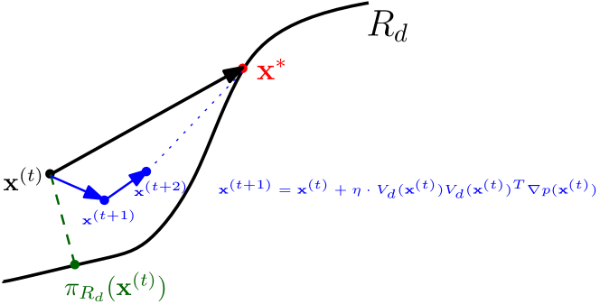
Figure 11: Decomposition of the vector $\bm{x}^{*}-\bm{x}^{(t)}$ into the summation $\sum\limits_{s=t}^{\infty}\left(\bm{x}^{(s+1)}-\bm{x}^{(s)}\right)$ of subspace constrained gradient ascent iterative vectors.

(b) We first decompose the vector $\bm{x}^{*}-\bm{x}^{(t)}$ into an infinite sum of SCGA iterations $\bm{x}^{(s+1)}=\bm{x}^{(s)}+\eta\cdot V_{d}(\bm{x}^{(s)})V_{d}(\bm{x}^{(s)})^{T}\nabla p(\bm{x}^{(s)})$ for $s\geq t$ and obtain that

$$\begin{split}&U_{d}^{\perp}(\bm{x}^{(t)})\left(\bm{x}^{*}-\bm{x}^{(t)}\right)\\ &=U_{d}^{\perp}(\bm{x}^{(t)})\cdot\sum_{s=t}^{\infty}\left(\bm{x}^{(s+1)}-\bm{x}^{(s)}\right)\\ &=\sum_{s=t}^{\infty}U_{d}^{\perp}(\bm{x}^{(t)})\cdot\eta V_{d}(\bm{x}^{(s)})V_{d}(\bm{x}^{(s)})^{T}\nabla p(\bm{x}^{(s)})\\ &\stackrel{{\scriptstyle\text{(i)}}}{{=}}\sum_{s=t}^{\infty}U_{d}^{\perp}(\bm{x}^{(t)})\cdot\eta\left[V_{d}(\bm{x}^{(s)})V_{d}(\bm{x}^{(s)})^{T}-V_{d}(\bm{x}^{(t)})V_{d}(\bm{x}^{(t)})^{T}\right]V_{d}(\bm{x}^{(s)})V_{d}(\bm{x}^{(s)})^{T}\nabla p(\bm{x}^{(s)})\end{split}$$ (65)

for any $\bm{x}^{(t)}\in R_{d}\oplus\rho$, where we leverage the orthogonality between $U_{d}^{\perp}(\bm{x}^{(t)})$ and $V_{d}(\bm{x}^{(t)})V_{d}(\bm{x}^{(t)})^{T}$ and the idempotence of $V_{d}(\bm{x}^{(s)})V_{d}(\bm{x}^{(s)})^{T}$ for all $s\geq t$ in (ii). See also Figure 11 for a graphical illustration of the decomposition. By Davis-Kahan theorem (Lemma D.1 and (60) here) and conditions (A1-2), we deduce that for all $s\geq t$,

$$\left|\left|V_{d}(\bm{x}^{(s)})V_{d}(\bm{x}^{(s)})^{T}-V_{d}(\bm{x}^{(t)})V_{d}(\bm{x}^{(t)})^{T}\right|\right|_{2}$$

$$\leq\frac{\sqrt{2}D\left|\left|\nabla\nabla p(\bm{x}^{(s)})-\nabla\nabla p(\bm{x}^{(t)})\right|\right|_{2}}{\beta_{0}}$$

$$\stackrel{{\scriptstyle\text{(i)}}}{{\leq}}\frac{\sqrt{2}D\left|\left|\nabla^{3}p(\bm{x}^{(t)})\right|\right|_{2}\left|\left|\bm{x}^{(s)}-\bm{x}^{(t)}\right|\right|_{2}}{\beta_{0}}+\frac{\sqrt{2}D^{3}\left|\left|p\right|\right|_{\infty}^{(4)}}{\beta_{0}}\cdot\left|\left|\bm{x}^{(s)}-\bm{x}^{(t)}\right|\right|_{2}^{2}$$

$$\stackrel{{\scriptstyle\text{(ii)}}}{{\leq}}\frac{2D^{\frac{5}{2}}\left|\left|\nabla^{3}p(\bm{x}^{(t)})\right|\right|_{\max}\left|\left|\bm{x}^{*}-\bm{x}^{(t)}\right|\right|_{2}}{\beta_{0}},$$

where we use the Taylor’s theorem in (i) as well as apply the self-contractedness condition (A5) and possibly shrink the radius $r_{5}>0$ so that $\left|\left|\bm{x}^{*}-\bm{x}^{(t)}\right|\right|_{2}\leq\frac{(2-\sqrt{2})\left|\left|\nabla^{3}p(\bm{x}^{(t)})\right|\right|_{\max}}{\sqrt{2D}\left|\left|p\right|\right|_{\infty}^{(4)}}$ in (ii). Hence, by (65) and the fact that $\left|\left|U_{d}^{\perp}(\bm{x}^{(t)})\right|\right|_{2}=1$, we obtain that

$$\left|\left|U_{d}^{\perp}(\bm{x}^{(t)})\left(\bm{x}^{*}-\bm{x}^{(t)}\right)\right|\right|_{2}$$

$$\leq\sup_{s\geq t}\left|\left|V_{d}(\bm{x}^{(s)})V_{d}(\bm{x}^{(s)})^{T}-V_{d}(\bm{x}^{(t)})V_{d}(\bm{x}^{(t)})^{T}\right|\right|_{2}\cdot\sum_{s=t}^{\infty}\left|\left|\eta V_{d}(\bm{x}^{(s)})V_{d}(\bm{x}^{(s)})^{T}\nabla p(\bm{x}^{(s)})\right|\right|_{2}$$

$$\leq\frac{2D^{\frac{5}{2}}\left|\left|\nabla^{3}p(\bm{x}^{(t)})\right|\right|_{\max}\left|\left|\bm{x}^{*}-\bm{x}^{(t)}\right|\right|_{2}}{\beta_{0}}\cdot 2^{10D^{2}}\left|\left|\bm{x}^{(t)}-\bm{x}^{*}\right|\right|_{2}$$

$$=\frac{2^{10D^{2}+1}D^{\frac{5}{2}}\left|\left|\nabla^{3}p(\bm{x}^{(t)})\right|\right|_{\max}\left|\left|\bm{x}^{*}-\bm{x}^{(t)}\right|\right|_{2}^{2}}{\beta_{0}},$$

implying the second bound in condition (A4) with $\beta_{2}=\frac{2^{10D^{2}+1}D^{\frac{5}{2}}\left|\left|p\right|\right|_{\infty}^{(3)}}{\beta_{0}}$. In addition,

$$\nabla p(\bm{x}^{(t)})^{T}U_{d}^{\perp}(\bm{x}^{(t)})(\bm{x}^{*}-\bm{x}^{(t)})$$

$$\leq\left|\left|U_{d}^{\perp}(\bm{x}^{(t)})\nabla p(\bm{x}^{(t)})\right|\right|_{2}\left|\left|U_{d}^{\perp}(\bm{x}^{(t)})\left(\bm{x}^{*}-\bm{x}^{(t)}\right)\right|\right|_{2}$$

$$\leq\frac{2^{10D^{2}+1}D^{\frac{5}{2}}\left|\left|U_{d}^{\perp}(\bm{x}^{(t)})\nabla p(\bm{x}^{(t)})\right|\right|_{2}\left|\left|\nabla^{3}p(\bm{x}^{(t)})\right|\right|_{\max}\left|\left|\bm{x}^{*}-\bm{x}^{(t)}\right|\right|_{2}^{2}}{\beta_{0}}.$$

The results follow. ∎

According to (b) of Lemma E.2, condition (A4) will hold with $\beta_{2}=\frac{2^{10D^{2}+1}D^{\frac{5}{2}}\left|\left|p\right|\right|_{\infty}^{(3)}}{\beta_{0}}$ whenever

$$2^{10D^{2}+1}D^{\frac{5}{2}}\left|\left|U_{d}^{\perp}(\bm{x}^{(t)})\nabla p(\bm{x}^{(t)})\right|\right|_{2}\left|\left|\nabla^{3}p(\bm{x}^{(t)})\right|\right|_{\max}\leq\frac{\beta_{0}^{2}}{4}.$$ (66)

The choice of $\beta_{2}>0$ is a valid constant under the differentiability condition (A1). More importantly, (66) is essentially the same assumption as the first inequality of condition (A3). Compared to the corresponding condition in (A3), the upper bound in (66) for $\left|\left|U_{d}^{\perp}(\bm{x}^{(t)})\nabla p(\bm{x}^{(t)})\right|\right|_{2}\left|\left|\nabla^{3}p(\bm{x}^{(t)})\right|\right|_{\max}$ around the ridge $R_{d}$ is only shrunk by a dimension-dependent factor $\frac{1}{D\cdot 2^{10D^{2}+2}}$. As condition (A3) and (66) are local, this adjustment does not induce too much extra strictness on the underlying density $p$.

E.2 Subspace Constrained Polyak-Łojasiewicz Inequality Assumption

We have demonstrated in Appendix E.1 that the crucial condition (A4) is valid under the self-contractedness assumption on the SCGA sequence $\big{\{}\bm{x}^{(t)}\big{\}}_{t=0}^{\infty}$. Consequently, the linear convergence of the SCGA algorithm can be established by slightly modifying the common assumptions (A1-3) in ridge estimation. Nevertheless, the self-contractedness property of the SCGA sequence $\big{\{}\bm{x}^{(t)}\big{\}}_{t=0}^{\infty}$ does not always hold in practice, and it may only be implied by the subspace constrained concavity condition (A6) as proved in Proposition E.1.

Given the fact that the underlying density function $p$ or its estimator $\widehat{p}_{n}$ may not satisfy the subspace constrained concavity assumption in many practical applications of SCGA and SCMS algorithms, we present another approach to deduce condition (A4) based on the well-known Polyak-Łojasiewicz inequality (Polyak, 1963; Lojasiewicz, 1963). Given any SCGA sequence $\big{\{}\bm{x}^{(t)}\big{\}}_{t=0}^{\infty}$ with limiting point $\bm{x}^{*}\in R_{d}$ and step size $0<\eta<\frac{2}{D\left|\left|p\right|\right|_{\infty}^{(2)}}$, we consider the following condition:

• (A7) (Subspace Constrained Polyak-Łojasiewicz Inequality) For all $t\geq 0$, there exists a constant $\beta_{3}>0$ such that

  $$\frac{1}{2}\left|\left|V_{d}(\bm{x}^{(t)})^{T}\nabla p(\bm{x}^{(t)})\right|\right|_{2}^{2}\geq\beta_{3}\left[p(\bm{x}^{*})-p(\bm{x}^{(t)})\right].$$

Similar to the standard Polyak-Łojasiewicz inequality, there exist some objective functions that satisfy the subspace constrained Polyak-Łojasiewicz inequality but fail to be concave in the subspace constrained sense as in condition (A6); see Charles and Papailiopoulos (2018); Fazel et al. (2018) and Equation (36) in Chen (2020). From this aspect, condition (A7) incorporates some extra SCGA sequences satisfying condition (A4) and converging linearly to the ridge $R_{d}$. However, as the subspace constrained Polyak-Łojasiewicz inequality does not imply condition (A5) or (A6), it should not be regarded as a more general condition. Furthermore, unlike the standard gradient ascent/descent method (Theorem 2 in Karimi et al. 2016), the error bound condition (i.e., Equation (59) here) does not imply the subspace constrained Polyak-Łojasiewicz inequality, indicating a challenge in validating condition (A7) in practice.

Despite these disadvantages, the subspace constrained Polyak-Łojasiewicz inequality condition does give rise to a concise proof for the linear convergence of the objective function value $\big{\{}p(\bm{x}^{(t)})\big{\}}_{t=0}^{\infty}$ along the SCGA sequence $\big{\{}\bm{x}^{(t)}\big{\}}_{t=0}^{\infty}$.

Proposition E.3.

Assume conditions (A1) and (A7). Then, for any SCGA sequence $\big{\{}\bm{x}^{(t)}\big{\}}_{t=0}^{\infty}$ with step size $0<\eta<\min\left\{\frac{1}{D\left|\left|p\right|\right|_{\infty}^{(2)}},\frac{1}{\beta_{3}}\right\}$, we have that

$$p(\bm{x}^{*})-p(\bm{x}^{(t)})\leq\big{[}p(\bm{x}^{*})-p(\bm{x}^{(0)})\big{]}\cdot(1-\eta\beta_{3})^{t}.$$

Proof of Proposition E.3.

The proof is inspired by Theorem 1 in Karimi et al. (2016). From (58) and condition (A7), we know that

$$p(\bm{x}^{(t+1)})-p(\bm{x}^{(t)}) \geq\eta\left(1-\frac{D\left|\left|p\right|\right|_{\infty}^{(2)}\eta}{2}\right)\left|\left|V_{d}(\bm{x}^{(t)})^{T}\nabla p(\bm{x}^{(t)})\right|\right|_{2}^{2}\geq\eta\beta_{3}\left[p(\bm{x}^{*})-p(\bm{x}^{(t)})\right]$$

for all $t\geq 0$ when $0<\eta<\frac{1}{D\left|\left|p\right|\right|_{\infty}^{(2)}}$. By some rearrangements, we conclude that

$$p(\bm{x}^{*})-p(\bm{x}^{(t+1)})\leq(1-\eta\beta_{3})\left[p(\bm{x}^{*})-p(\bm{x}^{(t)})\right].$$

The final display follows from telescoping. ∎

More importantly, the subspace constrained Polyak-Łojasiewicz inequality controls the total length of the SCGA path to be of the linear order and implicates the quadratic behaviors of residual vectors as required by condition (A4).

Lemma E.4.

Assume conditions (A1) and (A7) throughout the lemma.

1. The total length of the SCGA trajectory is of the linear order, i.e.,

   $$\sum_{s=t}^{\infty}\left|\left|\bm{x}^{(s+1)}-\bm{x}^{(s)}\right|\right|_{2}\leq\frac{4D\left|\left|p\right|\right|_{\infty}^{(2)}}{\beta_{3}}\left|\left|\bm{x}^{(t)}-\bm{x}^{*}\right|\right|_{2}\quad\text{ for any }t\geq 0.$$

2. We further assume condition (A2). Then,

   $$\nabla p(\bm{x}^{(t)})^{T}U_{d}^{\perp}(\bm{x}^{(t)})(\bm{x}^{*}-\bm{x}^{(t)})$$

   $$\leq\frac{32D^{\frac{9}{2}}\left(\left|\left|p\right|\right|_{\infty}^{(2)}\right)^{2}\left|\left|U_{d}^{\perp}(\bm{x}^{(t)})\nabla p(\bm{x}^{(t)})\right|\right|_{2}\left|\left|\nabla^{3}p(\bm{x}^{(t)})\right|\right|_{\max}\left|\left|\bm{x}^{*}-\bm{x}^{(t)}\right|\right|_{2}^{2}}{\beta_{0}\beta_{3}^{2}},$$

   and

   $$\left|\left|U_{d}^{\perp}(\bm{x}^{(t)})(\bm{x}^{*}-\bm{x}^{(t)})\right|\right|_{2}\leq\frac{32D^{\frac{9}{2}}\left(\left|\left|p\right|\right|_{\infty}^{(2)}\right)^{2}\left|\left|\nabla^{3}p(\bm{x}^{(t)})\right|\right|_{\max}\left|\left|\bm{x}^{*}-\bm{x}^{(t)}\right|\right|_{2}^{2}}{\beta_{0}\beta_{3}^{2}}$$

   for any $\bm{x}^{(t)}\in\text{Ball}_{D}(\bm{x}^{*},r_{6})$ with some radius $0<r_{6}<\rho$, where we recall that $\rho>0$ is the effective radius in condition (A2) under which the underlying density $p$ has an eigengap $\beta_{0}>0$ between the $d$-th and $(d+1)$-th eigenvalues of its Hessian matrix $\nabla\nabla p$.

Proof of Lemma E.4.

(a) This part of the proof is inspired by the arguments in Theorem 9 of Gupta et al. (2021). Based on the proof of (a) in Proposition 3.3 under condition (A1), we know from (58) that

$$p(\bm{x}^{(t+1)})-p(\bm{x}^{(t)}) \geq\eta\left(1-\frac{D\left|\left|p\right|\right|_{\infty}^{(2)}\eta}{2}\right)\left|\left|V_{d}(\bm{x}^{(t)})^{T}\nabla p(\bm{x}^{(t)})\right|\right|_{2}^{2}$$

$$\geq\frac{\eta}{2}\left|\left|V_{d}(\bm{x}^{(t)})^{T}\nabla p(\bm{x}^{(t)})\right|\right|_{2}^{2}$$

when $0<\eta<\frac{1}{D\left|\left|p\right|\right|_{\infty}^{(2)}}$. Using this inequality and condition (A7), we derive that

$$\sqrt{p(\bm{x}^{*})-p(\bm{x}^{(t+1)})} =\sqrt{p(\bm{x}^{*})-p\left(\bm{x}^{(t)}+\eta\cdot V_{d}(\bm{x}^{(t)})V_{d}(\bm{x}^{(t)})^{T}\nabla p(\bm{x}^{(t)})\right)}$$

$$\leq\sqrt{p(\bm{x}^{*})-p(\bm{x}^{(t)})-\frac{\eta}{2}\left|\left|V_{d}(\bm{x}^{(t)})^{T}\nabla p(\bm{x}^{(t)})\right|\right|_{2}^{2}}$$

$$\stackrel{{\scriptstyle\text{(i)}}}{{\leq}}\sqrt{p(\bm{x}^{*})-p(\bm{x}^{(t)})}-\frac{\eta\left|\left|V_{d}(\bm{x}^{(t)})^{T}\nabla p(\bm{x}^{(t)})\right|\right|_{2}^{2}}{4\sqrt{p(\bm{x}^{*})-p(\bm{x}^{(t)})}}$$

$$\stackrel{{\scriptstyle\text{(ii)}}}{{\leq}}\sqrt{p(\bm{x}^{*})-p(\bm{x}^{(t)})}-\frac{\eta\sqrt{2\beta_{3}}}{4}\left|\left|V_{d}(\bm{x}^{(t)})^{T}\nabla p(\bm{x}^{(t)})\right|\right|_{2},$$

where we use the inequality $\sqrt{a-b}\leq\sqrt{a}-\frac{b}{2\sqrt{a}}$ to obtain (i) and apply condition (A7) in inequality (ii). Since $\left|\left|\bm{x}^{(t+1)}-\bm{x}^{(t)}\right|\right|_{2}=\eta\left|\left|V_{d}(\bm{x}^{(t)})^{T}\nabla p(\bm{x}^{(t)})\right|\right|_{2}$, some rearrangement of the above inequality suggests that

$$\sqrt{\frac{\beta_{3}}{8}}\left|\left|\bm{x}^{(t+1)}-\bm{x}^{(t)}\right|\right|_{2}\leq\sqrt{p(\bm{x}^{*})-p(\bm{x}^{(t)})}-\sqrt{p(\bm{x}^{*})-p(\bm{x}^{(t+1)})}.$$

Therefore,

$$\sum_{s=t}^{\infty}\left|\left|\bm{x}^{(s+1)}-\bm{x}^{(s)}\right|\right|_{2} \leq\sqrt{\frac{8}{\beta_{3}}}\sum_{s=t}^{\infty}\left[\sqrt{p(\bm{x}^{*})-p(\bm{x}^{(s)})}-\sqrt{p(\bm{x}^{*})-p(\bm{x}^{(s+1)})}\right]$$

$$=\sqrt{\frac{8}{\beta_{3}}}\cdot\sqrt{p(\bm{x}^{*})-p(\bm{x}^{(t)})}$$

$$\stackrel{{\scriptstyle\text{(i)}}}{{\leq}}\sqrt{\frac{8}{\beta_{3}}}\cdot\sqrt{\frac{1}{2\beta_{3}}}\cdot\left|\left|V_{d}(\bm{x}^{(t)})^{T}\nabla p(\bm{x}^{(t)})\right|\right|_{2}\quad\text{ by condition (A4)}$$

$$=\frac{2}{\beta_{3}}\left|\left|V_{d}(\bm{x}^{(t)})^{T}\nabla p(\bm{x}^{(t)})-\underbrace{V_{d}(\bm{x}^{*})^{T}\nabla p(\bm{x}^{*})}_{=0}\right|\right|_{2}$$

$$\stackrel{{\scriptstyle\text{(ii)}}}{{\leq}}\frac{2}{\beta_{3}}\left|\left|\sup_{\epsilon\in[0,1]}M(\bm{x}^{*}+\epsilon(\bm{x}^{(t)}-\bm{x}^{*}))^{T}\left(\bm{x}^{(t)}-\bm{x}^{*}\right)\right|\right|_{2}$$

$$\stackrel{{\scriptstyle\text{(iii)}}}{{\leq}}\frac{2}{\beta_{3}}\left(D\left|\left|p\right|\right|_{\infty}^{(2)}+\beta_{0}-\beta_{1}\right)\left|\left|\bm{x}^{*}-\bm{x}^{(t)}\right|\right|_{2}$$

$$\leq\frac{4D\left|\left|p\right|\right|_{\infty}^{(2)}}{\beta_{3}}\left|\left|\bm{x}^{*}-\bm{x}^{(t)}\right|\right|_{2},$$

where we leverage condition (A7) again in (i). In addition, to obtain inequalities (ii) and (iii), we recall from the proof of (d) for Lemma C.1 that $M(\bm{x})=\nabla\left[V_{d}(\bm{x})^{T}\nabla p(\bm{x})\right]^{T}=V_{d}(\bm{x})\Lambda_{0}(\bm{x})+\sum_{i=1}^{d}T_{i}(\bm{x})V_{d}(\bm{x})\Lambda_{i}(\bm{x})$, in which the singular values of $V_{d}(\bm{x})\Lambda_{0}(\bm{x})$ is bounded by $D\left|\left|p\right|\right|_{\infty}^{(2)}$ and the singular values of $\sum_{i=1}^{d}T_{i}(\bm{x})V_{d}(\bm{x})\Lambda_{i}(\bm{x})$ is bounded by $\beta_{0}-\beta_{1}\leq D\left|\left|p\right|\right|_{\infty}^{(2)}$. The result thus follows.

(b) This part of the proof is analogous to our arguments in (b) of Lemma E.2, except that the SCGA sequence $\big{\{}\bm{x}^{(t)}\big{\}}_{t=0}^{\infty}$ is no longer self-contracted. For the completeness, we still repeat some arguments and highlight the differences here. By Davis-Kahan theorem (Lemma D.1 and (60) here) and conditions (A1-2), we have that for all $s\geq t$,

$$\left|\left|V_{d}(\bm{x}^{(s)})V_{d}(\bm{x}^{(s)})^{T}-V_{d}(\bm{x}^{(t)})V_{d}(\bm{x}^{(t)})^{T}\right|\right|_{2}$$

$$\leq\frac{\sqrt{2}D\left|\left|\nabla\nabla p(\bm{x}^{(s)})-\nabla\nabla p(\bm{x}^{(t)})\right|\right|_{2}}{\beta_{0}}$$

$$\leq\frac{\sqrt{2}D\left|\left|\nabla^{3}p(\bm{x}^{(t)})\right|\right|_{2}\left|\left|\bm{x}^{(s)}-\bm{x}^{(t)}\right|\right|_{2}}{\beta_{0}}+\frac{\sqrt{2}D^{3}\left|\left|p\right|\right|_{\infty}^{(4)}}{\beta_{0}}\left|\left|\bm{x}^{(s)}-\bm{x}^{(t)}\right|\right|_{2}^{2}$$

$$\stackrel{{\scriptstyle\text{(ii)}}}{{\leq}}\frac{4\sqrt{2}D^{2}\left|\left|p\right|\right|_{\infty}^{(2)}\left|\left|\nabla^{3}p(\bm{x}^{(t)})\right|\right|_{2}\left|\left|\bm{x}^{*}-\bm{x}^{(t)}\right|\right|_{2}}{\beta_{0}\beta_{3}}+\frac{16\sqrt{2}D^{5}\left|\left|p\right|\right|_{\infty}^{(4)}\left(\left|\left|p\right|\right|_{\infty}^{(2)}\right)^{2}}{\beta_{0}\beta_{3}^{2}}\left|\left|\bm{x}^{(t)}-\bm{x}^{*}\right|\right|_{2}^{2}$$

$$\stackrel{{\scriptstyle\text{(ii)}}}{{\leq}}\frac{8D^{\frac{7}{2}}\left|\left|p\right|\right|_{\infty}^{(2)}\left|\left|\nabla^{3}p(\bm{x}^{(t)})\right|\right|_{\max}\left|\left|\bm{x}^{*}-\bm{x}^{(t)}\right|\right|_{2}}{\beta_{0}\beta_{3}},$$

where we possibly shrink the radius $r_{6}>0$ so that $\left|\left|\bm{x}^{(t)}-\bm{x}^{*}\right|\right|_{2}\leq\frac{(\sqrt{2}-1)\beta_{3}\left|\left|\nabla^{3}p(\bm{x}^{(t)})\right|\right|_{\max}}{4D^{\frac{3}{2}}\left|\left|p\right|\right|_{\infty}^{(2)}\left|\left|p\right|\right|_{\infty}^{(4)}}$ to obtain inequality (ii). Notice also that, since $\left|\left|\bm{x}^{(s)}-\bm{x}^{(t)}\right|\right|_{2}\leq\left|\left|\bm{x}^{*}-\bm{x}^{(t)}\right|\right|_{2}$ may not hold without the self-contractedness property, we use a looser bound

$$\left|\left|\bm{x}^{(s)}-\bm{x}^{(t)}\right|\right|_{2}\leq\sum_{s=t}^{\infty}\left|\left|\bm{x}^{(s+1)}-\bm{x}^{(s)}\right|\right|_{2}\leq\frac{4D\left|\left|p\right|\right|_{\infty}^{(2)}}{\beta_{3}}\left|\left|\bm{x}^{(t)}-\bm{x}^{*}\right|\right|_{2}$$

from (a) to derive inequality (i). Therefore, by (65) and the fact that

$$\left|\left|\eta V_{d}(\bm{x}^{(s)})V_{d}(\bm{x}^{(s)})^{T}\nabla p(\bm{x}^{(s)})\right|\right|_{2}=\left|\left|\bm{x}^{(s+1)}-\bm{x}^{(s)}\right|\right|_{2},$$

we obtain that

$$\left|\left|U_{d}^{\perp}(\bm{x}^{(t)})\left(\bm{x}^{*}-\bm{x}^{(t)}\right)\right|\right|_{2}$$

$$\leq\sup_{s\geq t}\left|\left|V_{d}(\bm{x}^{(s)})V_{d}(\bm{x}^{(s)})^{T}-V_{d}(\bm{x}^{(t)})V_{d}(\bm{x}^{(t)})^{T}\right|\right|_{2}\cdot\sum_{s=t}^{\infty}\left|\left|\eta V_{d}(\bm{x}^{(s)})V_{d}(\bm{x}^{(s)})^{T}\nabla p(\bm{x}^{(s)})\right|\right|_{2}$$

$$\leq\frac{8D^{\frac{7}{2}}\left|\left|p\right|\right|_{\infty}^{(2)}\left|\left|\nabla^{3}p(\bm{x}^{(t)})\right|\right|_{\max}\left|\left|\bm{x}^{(s)}-\bm{x}^{(t)}\right|\right|_{2}}{\beta_{0}\beta_{3}}\cdot\frac{4D\left|\left|p\right|\right|_{\infty}^{(2)}}{\beta_{3}}\left|\left|\bm{x}^{(t)}-\bm{x}^{*}\right|\right|_{2}$$

$$=\frac{32D^{\frac{9}{2}}\left(\left|\left|p\right|\right|_{\infty}^{(2)}\right)^{2}\left|\left|\nabla^{3}p(\bm{x}^{(t)})\right|\right|_{\max}\left|\left|\bm{x}^{*}-\bm{x}^{(t)}\right|\right|_{2}^{2}}{\beta_{0}\beta_{3}^{2}},$$

which implies the second bound in condition (A4) with $\beta_{2}=\frac{32D^{\frac{9}{2}}\left(\left|\left|p\right|\right|_{\infty}^{(2)}\right)^{2}\left|\left|p\right|\right|_{\infty}^{(3)}}{\beta_{0}\beta_{3}^{2}}$. Finally,

$$\nabla p(\bm{x}^{(t)})^{T}U_{d}^{\perp}(\bm{x}^{(t)})(\bm{x}^{*}-\bm{x}^{(t)})$$

$$\leq\left|\left|U_{d}^{\perp}(\bm{x}^{(t)})\nabla p(\bm{x}^{(t)})\right|\right|_{2}\left|\left|U_{d}^{\perp}(\bm{x}^{(t)})\left(\bm{x}^{*}-\bm{x}^{(t)}\right)\right|\right|_{2}$$

$$\leq\frac{32D^{\frac{9}{2}}\left(\left|\left|p\right|\right|_{\infty}^{(2)}\right)^{2}\left|\left|U_{d}^{\perp}(\bm{x}^{(t)})\nabla p(\bm{x}^{(t)})\right|\right|_{2}\left|\left|\nabla^{3}p(\bm{x}^{(t)})\right|\right|_{\max}\left|\left|\bm{x}^{*}-\bm{x}^{(t)}\right|\right|_{2}^{2}}{\beta_{0}\beta_{3}^{2}}.$$

The results follow. ∎

The results in (b) of Lemma E.4 also imply condition (A4) with $\beta_{2}=\frac{32D^{\frac{9}{2}}\left(\left|\left|p\right|\right|_{\infty}^{(2)}\right)^{2}\left|\left|p\right|\right|_{\infty}^{(3)}}{\beta_{0}\beta_{3}^{2}}$ whenever

$$\frac{32D^{\frac{9}{2}}\left(\left|\left|p\right|\right|_{\infty}^{(2)}\right)^{2}\left|\left|U_{d}^{\perp}(\bm{x}^{(t)})\nabla p(\bm{x}^{(t)})\right|\right|_{2}\left|\left|\nabla^{3}p(\bm{x}^{(t)})\right|\right|_{\max}}{\beta_{3}^{2}}\leq\frac{\beta_{0}^{2}}{4}.$$ (67)

Once again, the choice of $\beta_{2}$ is feasible under condition (A1) and the upper bound (67) can be viewed as a variant of the first inequality in condition (A3). From this perspective, the subspace constrained Polyak-Łojasiewicz inequality (A7) also leads to an alternative assumptions for condition (A4) and the linear convergence of the SCGA algorithm.

Remark E.1.

Note that the results in Proposition E.4 can be generalized to the directional or arbitrary manifold cases under conditions (A1-3). First, the subspace constrained Polyak-Łojasiewicz inequality for the SCGA sequence $\big{\{}\underline{\bm{x}}^{(t)}\big{\}}_{t=0}^{\infty}$ on $\Omega_{q}$ or an arbitrary manifold can be modified as:

$$\frac{1}{2}\left|\left|\underline{V}_{d}(\underline{\bm{x}}^{(t)})^{T}\mathtt{grad}\,f(\underline{\bm{x}}^{(t)})\right|\right|_{2}^{2}\geq\underline{\beta}_{3}\left[f(\underline{\bm{x}}^{*})-f(\underline{\bm{x}}^{(t)})\right]\quad\text{ for some }\underline{\beta}_{3}>0\text{ and any }t\geq 0,$$

where $f$ is the objective (density) function. Based on the proof of (a) in Proposition 4.4 and our arguments in (a) of Lemma E.4, it follows that the total length of the SCGA trajectory on $\Omega_{q}$ or an arbitrary manifold is of the linear order, i.e.,

$$\sum_{s=t}^{\infty}d_{g}\left(\underline{\bm{x}}^{(s+1)},\underline{\bm{x}}^{(s)}\right)\leq\frac{4q\left|\left|\mathcal{H}f\right|\right|_{\infty}^{(2)}}{\underline{\beta}_{3}}\cdot d_{g}\left(\underline{\bm{x}}^{(t)},\underline{\bm{x}}^{*}\right)\quad\text{ for any }t\geq 0.$$

Second, to establish the quadratic bounds for $\left\langle\underline{U}_{d}^{\perp}(\underline{\bm{x}}^{(t)})\mathtt{grad}\,f(\underline{\bm{x}}^{(t)}),\,\mathtt{Exp}_{\underline{\bm{x}}^{(t)}}^{-1}(\underline{\bm{x}}^{*})\right\rangle$ and $\left|\left|\underline{U}_{d}^{\perp}(\underline{\bm{x}}^{(t)})\mathtt{Exp}_{\underline{\bm{x}}^{(t)}}^{-1}(\underline{\bm{x}}^{*})\right|\right|_{2}$, one can follow the arguments in the proof of (b) in Lemma E.4 and leverage the two facts:

1. The tangent vector $\mathtt{Exp}_{\underline{\bm{x}}^{(t)}}^{-1}(\underline{\bm{x}}^{*})$ can be decomposed into an infinite sum of SCGA updates (44) on $\Omega_{q}$ or an arbitrary manifold as:

$$\mathtt{Exp}_{\underline{\bm{x}}^{(t)}}^{-1}(\underline{\bm{x}}^{*}) =\sum_{s=t}^{\infty}\Gamma_{\underline{\bm{x}}^{(s)}}^{\underline{\bm{x}}^{(t)}}\left(\mathtt{Exp}_{\underline{\bm{x}}^{(s)}}^{-1}(\underline{\bm{x}}^{(s+1)})\right).$$

See Figure 12 for a graphical illustration. This equation is valid because parallel transports preserve inner products and are linear.

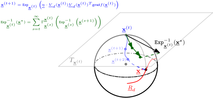
Figure 12: Decomposition of the vector $\mathtt{Exp}_{\underline{\bm{x}}^{(t)}}^{-1}(\underline{\bm{x}}^{*})$ within the tangent space $T_{\underline{\bm{x}}^{(t)}}$ into the summation $\sum\limits_{s=t}^{\infty}\Gamma_{\underline{\bm{x}}^{(s)}}^{\underline{\bm{x}}^{(t)}}\left(\mathtt{Exp}_{\underline{\bm{x}}^{(s)}}^{-1}(\underline{\bm{x}}^{(s+1)})\right)$ of parallel transported SCGA iterative vectors. Here, the blue curves on $\Omega_{q}$ are iterative paths of the SCGA algorithm, while the green vectors are tangent vectors $\mathtt{Exp}_{\underline{\bm{x}}^{(s)}}^{-1}(\underline{\bm{x}}^{(s+1)})\in T_{\underline{\bm{x}}^{(s)}}$ after being parallel transported to $T_{\underline{\bm{x}}^{(t)}}$.

2. Under conditions (A1-2), we know that

$$\left|\left|\underline{U}_{d}^{\perp}(\underline{\bm{x}}^{(t)})\cdot\sum_{s=t}^{\infty}\Gamma_{\underline{\bm{x}}^{(s)}}^{\underline{\bm{x}}^{(t)}}\left(\mathtt{Exp}_{\underline{\bm{x}}^{(s)}}^{-1}(\underline{\bm{x}}^{(s+1)})\right)\right|\right|_{2}$$

$$=\Bigg{\|}\sum_{s=t}^{\infty}\underline{U}_{d}^{\perp}(\underline{\bm{x}}^{(t)})\bigg{[}\Gamma_{\underline{\bm{x}}^{(s)}}^{\underline{\bm{x}}^{(t)}}\left(\underline{\eta}\underline{V}_{d}(\underline{\bm{x}}^{(s)})\underline{V}_{d}(\underline{\bm{x}}^{(s)})^{T}\underline{V}_{d}(\underline{\bm{x}}^{(s)})\underline{V}_{d}(\underline{\bm{x}}^{(s)})^{T}\mathtt{grad}\,f(\underline{\bm{x}}^{(s)})\right)$$

$$\hskip 56.9055pt-\underline{\eta}\underline{V}_{d}(\underline{\bm{x}}^{(t)})\underline{V}_{d}(\underline{\bm{x}}^{(t)})^{T}\underline{V}_{d}(\underline{\bm{x}}^{(s)})\underline{V}_{d}(\underline{\bm{x}}^{(s)})^{T}\mathtt{grad}\,f(\underline{\bm{x}}^{(s)})\bigg{]}\Bigg{\|}_{2}$$

$$\leq\sum_{s=t}^{\infty}\widetilde{A}\left|\left|\underline{V}_{d}(\underline{\bm{x}}^{(s)})\underline{V}_{d}(\underline{\bm{x}}^{(s)})^{T}-\underline{V}_{d}(\underline{\bm{x}}^{(t)})\underline{V}_{d}(\underline{\bm{x}}^{(t)})^{T}\right|\right|_{2}\cdot\left|\left|\underline{\bm{x}}^{(s)}-\underline{\bm{x}}^{(t)}\right|\right|_{2}$$

$$\leq\widetilde{A}\left|\left|\underline{\bm{x}}^{*}-\bm{x}^{(t)}\right|\right|_{2}\cdot\sum_{s=t}^{\infty}\left|\left|\underline{\bm{x}}^{(s)}-\underline{\bm{x}}^{(t)}\right|\right|_{2}$$

$$=O\left(\left|\left|\underline{\bm{x}}^{(s)}-\underline{\bm{x}}^{(t)}\right|\right|_{2}^{2}\right)$$

for some constant $\underline{A}>0$, where we leverage the fact that the vector field

$$X(\gamma(t))=\underline{V}_{d}(\gamma(t))\underline{V}_{d}(\gamma(t))^{T}\underline{V}_{d}(\underline{\bm{x}}^{(s)})\underline{V}_{d}(\underline{\bm{x}}^{(s)})^{T}\mathtt{grad}\,f(\underline{\bm{x}}^{(s)})$$

with $\gamma(0)=\underline{\bm{x}}^{(s)}$ and $\gamma(1)=\underline{\bm{x}}^{(t)}$ has its variation $\left|\left|X(\gamma(t_{1}))-X(\gamma(t_{2}))\right|\right|_{2}$ bounded by

$$\left|\left|\underline{V}_{d}(\underline{\bm{x}}^{(s)})\underline{V}_{d}(\underline{\bm{x}}^{(s)})^{T}-\underline{V}_{d}(\underline{\bm{x}}^{(t)})\underline{V}_{d}(\underline{\bm{x}}^{(t)})^{T}\right|\right|_{2}=O\left(\left|\left|\underline{\bm{x}}^{(s)}-\underline{\bm{x}}^{(t)}\right|\right|_{2}\right)$$

according to the Davis-Kahan theorem for any $0\leq t_{1},t_{2}\leq 1$. However, we are not sure if the self-contractedness condition can also be adaptive to the directional or general manifold cases, given that the arguments in Theorem 15 of Gupta et al. (2021) are based on the Euclidean geometry.

Appendix F Other Technical Concepts of Differential Geometry on $\Omega_{q}$

$\bullet$ Taylor’s Theorem on $\Omega_{q}$. Given a smooth function $f$ on $\Omega_{q}$, its Taylor’s expansion is often written as (Pennec, 2006):

$$f(\mathtt{Exp}_{\bm{x}}(\bm{v}))=f(\bm{x})+\left\langle\mathtt{grad}\,f(\bm{x}),\bm{v}\right\rangle+\frac{1}{2}\bm{v}^{T}\mathcal{H}f(\bm{x})\bm{v}+o\left(\left|\left|\bm{v}\right|\right|_{2}^{2}\right)$$ (68)

for any $\bm{v}\in T_{\bm{x}}$, where $\mathtt{Exp}_{\bm{x}}:T_{\bm{x}}\to\Omega_{q}$ is the exponential map at $\bm{x}\in\Omega_{q}$. One may replace the exponential map with a more general concept called the retractions on an arbitrary manifold; see Section 4.1 and Proposition 5.5.5 in Absil et al. (2008).

$\bullet$ Parallel Transport. When comparing vectors in two different tangent spaces $T_{\bm{x}},T_{\bm{y}}$ on $\Omega_{q}$, we leverage the notion of parallel transport $\Gamma_{\bm{x}}^{\bm{y}}:T_{\bm{x}}\to T_{\bm{y}}$ to transport vectors from one tangent space to another along a geodesic. In addition, $\Gamma_{\bm{x}}^{\bm{y}}(\bm{v})$ is a tangent vector in $T_{\bm{y}}$ after being parallel transported from $\bm{v}\in T_{\bm{x}}$ along a geodesic (or great circle) on $\Omega_{q}$. The parallel transport mapping $\Gamma_{\bm{x}}^{\bm{y}}$ is a linear isometry along any smooth curve on $\Omega_{q}$, i.e., $\left\langle\Gamma_{\bm{x}}^{\bm{y}}(\bm{u}),\Gamma_{\bm{x}}^{\bm{y}}(\bm{v})\right\rangle=\langle\bm{u},\bm{v}\rangle$ for any $\bm{u},\bm{v}\in T_{\bm{x}}$; see Proposition 5.5 in Lee (2018) or Proposition 1 in Section 4-4 of do Carmo (2016).

$\bullet$ Sectional Curvature. Sectional curvature is the Gaussian curvature of a two-dimensional submanifold formed as the image of a two-dimensional subspace of a tangent space after exponential mapping; see Section 3-2 in do Carmo (2016) for detailed discussions about the Gaussian curvature. It is known that a two dimensional submanifold with positive, zero, or negative sectional curvature is locally isometric to a two dimensional sphere, a Euclidean plane, or a hyperbolic plane with the same Gaussian curvature (Zhang and Sra, 2016).

$\bullet$ Geodesically Strong Concavity. A function $f:\Omega_{q}\to\mathbb{R}$ is said to be geodesically concave if for any $\bm{x},\bm{y}\in\Omega_{q}$, it holds that

$$f(\varphi(t))\geq(1-t)f(\bm{x})+f(\bm{y})$$

for any $t\in[0,1]$, where $\varphi:[0,1]\to\Omega_{q}$ is a geodesic with $\varphi(0)=\bm{x}$ and $\varphi(1)=\bm{y}$. When $f$ is differentiable, an equivalent statement of the geodesic concavity is that (Theorem 11.17 in Boumal 2020):

$$f(\bm{y})-f(\bm{x})\leq\left\langle\mathtt{grad}\,f(\bm{x}),\mathtt{Exp}_{\bm{x}}^{-1}(\bm{y})\right\rangle.$$

A function $f:\Omega_{q}\to\mathbb{R}$ is said to be geodesically $\mu_{g}$-strongly concave if for any $\bm{x},\bm{y}\in\Omega_{q}$, it holds that

$$f(\bm{y})\leq f(\bm{x})+\left\langle\mathtt{grad}\,f(\bm{x}),\mathtt{Exp}_{\bm{x}}^{-1}(\bm{y})\right\rangle-\frac{\mu_{g}}{2}\cdot d_{g}(\bm{x},\bm{y})^{2}.$$

Appendix G Normal Space of Directional Density Ridge

Recall that we extend the directional density $f$ from its support $\Omega_{q}$ to $\mathbb{R}^{q+1}\setminus\left\{\bm{0}\right\}$ by defining $f(\bm{x})\equiv f\left(\frac{\bm{x}}{\left|\left|\bm{x}\right|\right|_{2}}\right)$ for all $\bm{x}\in\mathbb{R}^{q+1}\setminus\left\{\bm{0}\right\}$. As we will refer to conditions (A1-3) frequently in the next three sections, we restate them here:

• (A1) (Differentiability) Under the extension (27) of the directional density $f$, we assume that the total gradient $\nabla f(\bm{x})$, total Hessian matrix $\nabla\nabla f(\bm{x})$, and third-order derivative tensor $\nabla^{3}f(\bm{x})$ in $\mathbb{R}^{q+1}$ exist, and are continuous on $\mathbb{R}^{q+1}\setminus\{\bm{0}\}$ and square integrable on $\Omega_{q}$. We also assume that $f$ has bounded fourth order derivatives on $\Omega_{q}$.

• (A2) (Eigengap) We assume that there exist constants $\underline{\rho}>0$ and $\underline{\beta}_{0}>0$ such that $\underline{\lambda}_{d+1}(\bm{y})\leq-\underline{\beta}_{0}$ and $\underline{\lambda}_{d}(\bm{y})-\underline{\lambda}_{d+1}(\bm{y})\geq\underline{\beta}_{0}$ for any $\bm{y}\in\left(\underline{R}_{d}\oplus\underline{\rho}\right)\cap\Omega_{q}$.

• (A3) (Path Smoothness) Under the same $\underline{\rho},\underline{\beta}_{0}>0$ in (A2), we assume that there exists another constant $\underline{\beta}_{1}\in\left(0,\underline{\beta}_{0}\right)$ such that

  $$\sqrt{2}\cdot q^{\frac{3}{2}}\left|\left|\underline{U}_{d}^{\perp}(\bm{y})\mathtt{grad}\,f(\bm{y})\right|\right|_{2}\left|\left|\nabla^{3}f(\bm{y})\right|\right|_{\max} \leq\frac{\underline{\beta}_{0}^{2}}{2},$$

  $$d\cdot q^{\frac{3}{2}}\left|\left|\nabla f(\bm{x})\right|\right|_{2}\cdot\left|\left|\nabla^{3}f(\bm{x})\right|\right|_{\max} \leq\underline{\beta}_{0}\left(\underline{\beta}_{0}-\underline{\beta}_{1}\right)$$

  for all $\bm{y}\in\left(\underline{R}_{d}\oplus\underline{\rho}\right)\cap\Omega_{q}$ and $\bm{x}\in\underline{R}_{d}$.

Recall that an order-$d$ density ridge of a directional density $f$ on $\Omega_{q}=\left\{\bm{x}\in\mathbb{R}^{q+1}:\left|\left|\bm{x}\right|\right|_{2}=1\right\}$ is the set of points defined as:

$$\underline{R}_{d}=\left\{\bm{x}\in\Omega_{q}:\underline{G}_{d}(\bm{x})=\bm{0},\underline{\lambda}_{d+1}(\bm{x})<0\right\}=\left\{\bm{x}\in\Omega_{q}:\underline{V}_{d}(\bm{x})^{T}\mathtt{grad}\,f(\bm{x})=\bm{0},\underline{\lambda}_{d+1}(\bm{x})<0\right\}.$$ (69)

Lemma G.1 below shows that under conditions (A1-3), the Jacobian matrices $\nabla\left[\underline{V}_{d}(\bm{x})^{T}\mathtt{grad}\,f(\bm{x})\right]\in\mathbb{R}^{(q-d)\times(q+1)}$ and $\left(\bm{I}_{q+1}-\bm{x}\bm{x}^{T}\right)\nabla\left[\underline{V}_{d}(\bm{x})^{T}\mathtt{grad}\,f(\bm{x})\right]^{T}\in\mathbb{R}^{(q+1)\times(q-d)}$ (i.e., projecting the columns of $\nabla\left[\underline{V}_{d}(\bm{x})^{T}\mathtt{grad}\,f(\bm{x})\right]^{T}$ onto the tangent space $T_{\bm{x}}$) both have rank $q-d$ at every point on $\underline{R}_{d}$, and $\underline{R}_{d}$ will be a $d$-dimensional submanifold on $\Omega_{q}$ by the implicit function theorem (Rudin, 1976; Lee, 2012). Analogous to the discussion about the normal space of a Euclidean density ridge in Appendix C, we define

$$\underline{M}(\bm{x})=\nabla\left[\underline{V}_{d}(\bm{x})^{T}\mathtt{grad}\,f(\bm{x})\right]^{T} =\nabla\left[\underline{V}_{d}(\bm{x})^{T}\nabla f(\bm{x})\right]^{T}$$

$$=\left(\underline{\bm{m}}_{d+1}(\bm{x}),...,\underline{\bm{m}}_{q}(\bm{x})\right)\in\mathbb{R}^{(q+1)\times(q-d)}.$$

Different from the Euclidean density ridge case, it is the column space of

$$\underline{M}_{E}(\bm{x})=\left(\nabla\left[\underline{V}_{d}(\bm{x})^{T}\nabla f(\bm{x})\right]^{T},\bm{x}\right)=\left(\underline{\bm{m}}_{d+1}(\bm{x}),...,\underline{\bm{m}}_{q}(\bm{x}),\bm{x}\right)\in\mathbb{R}^{(q+1)\times(q+1-d)}$$ (70)

that spans the normal space of $\underline{R}_{d}$ within the ambient space $\mathbb{R}^{q+1}$. It can be seen from our Remark 4.1 that the rows of

$$\nabla\Psi(\bm{x})=\begin{pmatrix}\nabla\left[\underline{\bm{v}}_{d+1}(\bm{x})^{T}\nabla f(\bm{x})\right]\\ \vdots\\ \nabla\left[\underline{\bm{v}}_{q}(\bm{x})^{T}\nabla f(\bm{x})\right]\\ 2\bm{x}\end{pmatrix}$$

spans the normal space of the solution manifold $\underline{R}_{d}$; see also Lemma 1 in Chen (2020). Consequently, the column space of $\left(\bm{I}_{q+1}-\bm{x}\bm{x}^{T}\right)\underline{M}(\bm{x})=\left(\bm{I}_{q+1}-\bm{x}\bm{x}^{T}\right)\nabla\left[\underline{V}_{d}(\bm{x})^{T}\mathtt{grad}\,f(\bm{x})\right]^{T}$ spans the normal space of $\underline{R}_{d}$ within the tangent space $T_{\bm{x}}$ at each $\bm{x}\in\underline{R}_{d}\subset\Omega_{q}$. The technique in pages 60-63 of Eberly (1996) is still valid to argue that

$$\begin{split}&\underline{\bm{m}}_{k}(\bm{x})\\ &=\left[\underline{\lambda}_{k}(\bm{x})\bm{I}_{q+1}+\sum_{i=1}^{d}\frac{\underline{\bm{v}}_{i}(\bm{x})^{T}\nabla f(\bm{x})}{\underline{\lambda}_{k}(\bm{x})-\underline{\lambda}_{i}(\bm{x})}\cdot\underline{\bm{v}}_{i}(\bm{x})^{T}\nabla^{3}f(\bm{x})+\frac{\bm{x}^{T}\nabla f(\bm{x})}{\underline{\lambda}_{k}(\bm{x})}\cdot\bm{x}^{T}\nabla^{3}f(\bm{x})\right]\underline{\bm{v}}_{k}(\bm{x})\\ &=\left[\underline{\lambda}_{k}(\bm{x})\bm{I}_{q+1}+\sum_{i=1}^{d}\frac{\underline{\bm{v}}_{i}(\bm{x})^{T}\nabla f(\bm{x})}{\underline{\lambda}_{k}(\bm{x})-\underline{\lambda}_{i}(\bm{x})}\cdot\underline{\bm{v}}_{i}(\bm{x})^{T}\nabla^{3}f(\bm{x})\right]\underline{\bm{v}}_{k}(\bm{x})\end{split}$$ (71)

for $k=d+1,...,q$, where we use the fact that $\bm{x}^{T}\nabla f(\bm{x})=\bm{x}^{T}\mathtt{grad}\,f(\bm{x})=0$ on $\Omega_{q}$ under the extension of $f$ as in (A1). Let

$$\underline{\Lambda}_{0}(\bm{x}) =\mathtt{Diag}\left[\underline{\lambda}_{d+1}(\bm{x}),...,\underline{\lambda}_{q}(\bm{x})\right],$$

$$\underline{\Lambda}_{i}(\bm{x}) =\mathtt{Diag}\left[\frac{1}{\underline{\lambda}_{d+1}(\bm{x})-\underline{\lambda}_{i}(\bm{x})},...,\frac{1}{\underline{\lambda}_{q}(\bm{x})-\underline{\lambda}_{i}(\bm{x})}\right],$$

$$\underline{T}_{i}(\bm{x}) =\left[\underline{\bm{v}}_{i}(\bm{x})^{T}\nabla f(\bm{x})\right]\cdot\underline{\bm{v}}_{i}(\bm{x})^{T}\nabla^{3}f(\bm{x})$$

for $i=1,...,d$. Then,

$$\underline{M}(\bm{x})=\underline{V}_{d}(\bm{x})\underline{\Lambda}_{0}(\bm{x})+\sum_{i=1}^{d}\underline{T}_{i}(\bm{x})\underline{V}_{d}(\bm{x})\underline{\Lambda}_{i}(\bm{x}).$$ (72)

As in the Euclidean data case, the columns of $\underline{M}_{E}(\bm{x})=\left[\underline{M}(\bm{x}),\bm{x}\right]\in\mathbb{R}^{(q+1)\times(q+1-d)}$ are not orthonormal, and we again leverage the orthonormalization technique in Chen et al. (2015) to construct $\underline{N}(\bm{x})$ that shares the same column space with $\underline{M}_{E}(\bm{x})$ but has orthonormal columns. That is, under the condition that $\underline{M}_{E}(\bm{x})$ has full column rank $q-d$ at every point $\bm{x}\in\underline{R}_{d}$ (see Lemma G.1),

$$\underline{N}(\bm{x})=\underline{M}_{E}(\bm{x})\left[\underline{J}(\bm{x})^{T}\right]^{-1}$$ (73)

with the Cholesky decomposition $\underline{M}_{E}(\bm{x})^{T}\underline{M}_{E}(\bm{x})=\underline{J}(\bm{x})\underline{J}(\bm{x})^{T}$, where $\underline{J}(\bm{x})\in\mathbb{R}^{(q+1-d)\times(q+1-d)}$ is a lower triangular matrix whose diagonal elements are positive. Finally, the non-uniqueness of $\underline{M}_{E}(\bm{x})$ will not affect our subsequent discussions about the properties of directional density ridges.

Lemma G.1.

Assume conditions (A1-3). Given that $\underline{M}(\bm{x})$, $\underline{M}_{E}(\bm{x})=\left[\underline{M}(\bm{x}),\bm{x}\right]$, and $\underline{N}(\bm{x})$ are defined in (72) and (73), we have the following properties:

1. $\underline{M}_{E}(\bm{x})$ and $\underline{N}(\bm{x})$ have the same column space. In addition,

   $$\underline{N}(\bm{x})\underline{N}(\bm{x})^{T}=\underline{M}_{E}(\bm{x})\left[\underline{M}_{E}(\bm{x})^{T}\underline{M}_{E}(\bm{x})\right]^{-1}\underline{M}_{E}(\bm{x})^{T}.$$

   That is, $\underline{N}(\bm{x})\underline{N}(\bm{x})^{T}$ is the projection matrix onto the columns of $\underline{M}_{E}(\bm{x})$.

2. The columns of $\underline{N}(\bm{x})$ are orthonormal to each other.

3. For $\bm{x}\in\underline{R}_{d}$, the column space of $\underline{N}(\bm{x})$ is normal to the (tangent) direction of $\underline{R}_{d}$ at $\bm{x}$.

4. For $\bm{x}\in\underline{R}_{d}$, the smallest eigenvalue $\lambda_{\min}(\underline{M}(\bm{x})^{T}\underline{M}(\bm{x}))=\lambda_{\min}(\underline{M}(\bm{x})^{T}(\bm{I}_{q+1}-\bm{x}\bm{x}^{T})\underline{M}(\bm{x}))\geq\underline{\beta}_{1}^{2}>0$, and

   $$\mathtt{rank}(\underline{M}(\bm{x}))=\mathtt{rank}\left((\bm{I}_{q+1}-\bm{x}\bm{x}^{T})\underline{M}(\bm{x})\right)=q-d.$$

   Moreover, all the nonzero singular values of $\underline{M}_{E}(\bm{x})$ are greater than $\min\left\{\underline{\beta}_{1},1\right\}>0$, and

   $$\mathtt{rank}(\underline{N}(\bm{x}))=\mathtt{rank}(\underline{M}_{E}(\bm{x}))=q+1-d.$$

   Therefore, $\underline{R}_{d}$ is a $d$-dimensional submanifold that contains neither intersections and nor endpoints on $\Omega_{q}$. Namely, $\underline{R}_{d}$ is a finite union of connected and compact submanifolds on $\Omega_{q}$.

5. For all $\bm{x}\in\underline{R}_{d}$,

   $$\left|\left|\left[\underline{M}(\bm{x})^{T}\left(\bm{I}_{q+1}-\bm{x}\bm{x}^{T}\right)\underline{M}(\bm{x})\right]^{-1}\right|\right|_{2}\leq\frac{1}{\underline{\beta}_{1}^{2}}\quad\text{ and }\quad\left|\left|\left[\underline{J}(\bm{x})^{T}\right]^{-1}\right|\right|_{2}\leq\max\left\{\frac{1}{\underline{\beta}_{1}},1\right\}.$$

6. When $\left|\left|\bm{x}-\bm{y}\right|\right|_{2}$ is sufficiently small and $\bm{x},\bm{y}\in\left(\underline{R}_{d}\oplus\underline{\rho}\right)\cap\Omega_{q}$,

   $$\left|\left|\underline{N}(\bm{x})\underline{N}(\bm{x})^{T}-\underline{N}(\bm{y})\underline{N}(\bm{y})^{T}\right|\right|_{\max}\leq\underline{A}_{0}\left(\left|\left|f\right|\right|_{\infty}^{(3)}+\left|\left|f\right|\right|_{\infty}^{(4)}\right)^{2}\left|\left|\bm{x}-\bm{y}\right|\right|_{2}$$

   for some constant $\underline{A}_{0}>0$.

7. Assume that another directional density function $g$ also satisfies conditions (A1-3) after the extension $g(\bm{x})\equiv g\left(\frac{\bm{x}}{\left|\left|\bm{x}\right|\right|}\right)$ in $\mathbb{R}^{q+1}\setminus\{\bm{0}\}$, and $\left|\left|f-g\right|\right|_{\infty,3}^{*}$ is sufficiently small. Then,

   $$\left|\left|\underline{N}_{f}(\bm{x})\underline{N}_{f}(\bm{x})^{T}-\underline{N}_{g}(\bm{x})\underline{N}_{g}(\bm{x})^{T}\right|\right|_{\max}\leq\underline{A}_{1}\cdot\left|\left|f-g\right|\right|_{\infty,3}^{*}$$

   for some constant $\underline{A}_{1}>0$ and any $\bm{x}\in\underline{R}_{d}$, where $\underline{N}_{f}(\bm{x})$ is the matrix defined in (73) with directional density $f$.

8. The reach of $\underline{R}_{d}$ satisfies

   $$\mathtt{reach}(\underline{R}_{d})\geq\min\left\{\underline{\rho}/2,\frac{\min\left\{\underline{\beta}_{1},1\right\}^{2}}{\underline{A}_{2}\left(\left|\left|f\right|\right|_{\infty}^{(3)}+\left|\left|f\right|\right|_{\infty}^{(4)}\right)}\right\}$$

   for some constant $\underline{A}_{2}>0$.

This lemma is a direct extension of Lemma C.1 to the directional data scenario; thus, its proof is similar to the proof of Lemma C.1.

Proof of Lemma G.1.

The proofs of properties (a), (b), and (c) can be inherited from the corresponding ones in Lemma C.1 with mild modifications and we thus omit them.

(d) We will prove that the $(q-d)$ nonzero singular values of $\underline{M}(\bm{x})$ and $\left(\bm{I}_{q+1}-\bm{x}\bm{x}^{T}\right)\underline{M}(\bm{x})\in\mathbb{R}^{(q+1)\times(q-d)}$ are bounded away from 0. Recall that

$$\underline{M}(\bm{x})=\underline{V}_{d}(\bm{x})\underline{\Lambda}_{0}(\bm{x})+\sum_{i=1}^{d}\underline{T}_{i}(\bm{x})\underline{V}_{d}(\bm{x})\underline{\Lambda}_{i}(\bm{x})$$

with

$$\underline{\Lambda}_{0}(\bm{x}) =\mathtt{Diag}\left[\underline{\lambda}_{d+1}(\bm{x}),...,\underline{\lambda}_{q}(\bm{x})\right]$$

$$\underline{\Lambda}_{i}(\bm{x}) =\mathtt{Diag}\left[\frac{1}{\underline{\lambda}_{d+1}(\bm{x})-\underline{\lambda}_{i}(\bm{x})},...,\frac{1}{\underline{\lambda}_{q}(\bm{x})-\underline{\lambda}_{i}(\bm{x})}\right]$$

$$\underline{T}_{i}(\bm{x}) =\left[\underline{\bm{v}}_{i}(\bm{x})^{T}\nabla f(\bm{x})\right]\cdot\underline{\bm{v}}_{i}(\bm{x})^{T}\nabla^{3}f(\bm{x})$$

for $i=1,...,d$. Under condition (A2),

$$\left|\left|\left(\bm{I}_{q+1}-\bm{x}\bm{x}^{T}\right)\cdot\sum_{i=1}^{d}\underline{T}_{i}(\bm{x})\underline{V}_{d}(\bm{x})\underline{\Lambda}_{i}(\bm{x})\right|\right|_{2}$$

$$\leq\left|\left|\sum_{i=1}^{d}\underline{T}_{i}(\bm{x})\underline{V}_{d}(\bm{x})\underline{\Lambda}_{i}(\bm{x})\right|\right|_{2}\quad\text{ since }\left|\left|\bm{I}_{q+1}-\bm{x}\bm{x}^{T}\right|\right|_{2}=1$$

$$\leq\sum_{i=1}^{d}\left|\left|\underline{T}_{i}(\bm{x})\right|\right|_{2}\cdot\left|\left|\underline{V}_{d}(\bm{x})\right|\right|_{2}\cdot\frac{1}{\underline{\beta}_{0}}\quad\text{ by (\text@underline{A2})}$$

$$\leq\sum_{i=1}^{d}\left|\left|\underline{\bm{v}}_{i}(\bm{x})^{T}\nabla f(\bm{x})\right|\right|_{2}\cdot\left|\left|\underline{\bm{v}}_{i}(\bm{x})^{T}\nabla^{3}f(\bm{x})\right|\right|_{2}\quad\text{ since }\left|\left|\underline{V}_{d}(\bm{x})\right|\right|_{2}=1$$

$$\leq\frac{d\left|\left|\nabla f(\bm{x})\right|\right|_{2}\cdot q^{\frac{3}{2}}\left|\left|\nabla^{3}f(\bm{x})\right|\right|_{\max}}{\underline{\beta}_{0}}$$

$$\leq\underline{\beta}_{0}-\underline{\beta}_{1}.$$

It shows that all the singular values of $\left(\bm{I}_{q+1}-\bm{x}\bm{x}^{T}\right)\sum\limits_{i=1}^{d}\underline{T}_{i}(\bm{x})\underline{V}_{d}(\bm{x})\underline{\Lambda}_{i}(\bm{x})$ or simply $\sum\limits_{i=1}^{d}\underline{T}_{i}(\bm{x})\underline{V}_{d}(\bm{x})\underline{\Lambda}_{i}(\bm{x})$ are less than $\underline{\beta}_{0}-\underline{\beta}_{1}$. Moreover, under condition (A2) again, all the $(q-d)$ singular values of

$$\left(\bm{I}_{q+1}-\bm{x}\bm{x}^{T}\right)\underline{V}_{d}(\bm{x})\underline{\Lambda}_{0}(\bm{x})=\underline{V}_{d}(\bm{x})\underline{\Lambda}_{0}(\bm{x})$$

are greater than $\underline{\beta}_{1}$.
By Theorem 3.3.16 in Horn and Johnson (1991), we know that all the singular values of $\underline{M}(\bm{x})$ and $\left(\bm{I}_{q+1}-\bm{x}\bm{x}^{T}\right)\underline{M}(\bm{x})$ are greater than

$$\sigma_{i}\left(\underline{V}_{d}(\bm{x})\underline{\Lambda}_{0}(\bm{x})\right)-\sigma_{1}\left(\sum_{i=1}^{d}\underline{T}_{i}(\bm{x})\underline{V}_{d}(\bm{x})\underline{\Lambda}_{i}(\bm{x})\right)\geq\underline{\beta}_{0}-(\underline{\beta}_{0}-\underline{\beta}_{1})=\underline{\beta}_{1}>0,$$

where $\sigma_{i}(A),i=1,...,q-d$ are singular values of a matrix $A\in\mathbb{R}^{(q+1)\times(q-d)}$ in their descending order. Therefore, the minimum eigenvalue of $\underline{M}(\bm{x})^{T}\underline{M}(\bm{x})$ satisfies

$$\lambda_{\min}\left(\underline{M}(\bm{x})^{T}\underline{M}(\bm{x})\right)=\lambda_{\min}\left(\underline{M}(\bm{x})^{T}(\bm{I}_{q+1}-\bm{x}\bm{x}^{T})\underline{M}(\bm{x})\right)\geq\underline{\beta}_{1}^{2}>0.$$ (74)

Now, given $\underline{M}_{E}(\bm{x})=\left[\underline{M}(\bm{x}),\bm{x}\right]\in\mathbb{R}^{(q+1)\times(q+1-d)}$ and $\bm{x}\in\Omega_{q}$, we know that

$$\underline{M}_{E}(\bm{x})^{T}\underline{M}_{E}(\bm{x})=\begin{pmatrix}\underline{M}(\bm{x})^{T}\underline{M}(\bm{x})&\underline{M}(\bm{x})^{T}\bm{x}\\ \bm{x}^{T}\underline{M}(\bm{x})&1\end{pmatrix}.$$

If we denote the orthonormal eigenvectors of $\underline{M}(\bm{x})^{T}\underline{M}(\bm{x})$ by $\bm{v}_{\underline{M},1}(\bm{x}),...,\bm{v}_{\underline{M},q-d}(\bm{x})\in\mathbb{R}^{q-d}$, then

$$\begin{pmatrix}\bm{v}_{\underline{M},1}(\bm{x})\\ 0\end{pmatrix},...,\begin{pmatrix}\bm{v}_{\underline{M},q-d}(\bm{x})\\ 0\end{pmatrix},\begin{pmatrix}\bm{0}\\ 1\end{pmatrix}\in\mathbb{R}^{q+1-d}$$

are the orthonormal eigenvectors of $\underline{M}_{E}(\bm{x})^{T}\underline{M}_{E}(\bm{x})$, whose eigenvalues are thus lower bounded by $\min\left\{\underline{\beta}_{1},1\right\}$ due to (74). Hence, $\mathtt{rank}(\underline{N}(\bm{x}))=\mathtt{rank}(\underline{M}_{E}(\bm{x}))=q+1-d$.
By the implicit function theorem and the extra constraint $\underline{R}_{d}\subset\Omega_{q}$, $\underline{R}_{d}$ is a $d$-dimensional submanifold on $\Omega_{q}$. It also implies that $\underline{R}_{d}$ cannot have intersections, because otherwise the intersected points will violate the rank condition.
Finally, we argue by contradiction that $\underline{R}_{d}$ has no endpoints. Assume, on the contrary, that $\underline{R}_{d}$ has an end point $\bm{x}_{0}$. Our preceding argument has shown that $\underline{M}(\bm{x})$, the derivative of $\underline{V}_{d}(\bm{x})^{T}\nabla f(\bm{x})$, is bounded. In addition, $\bm{x}_{0}\in\underline{R}_{d}$. However, this contradicts to the implicit function theorem indicating that $\underline{R}_{d}$ is a $d$-dimensional submanifold on $\Omega_{q}$, because at the end point $\bm{x}_{0}\in\underline{R}_{d}$, there exists no local coordinate chart for $\underline{R}_{d}$ defined on an open set in $\underline{R}_{d}$. The results follow.

(e) By the proof of (d), we already know that all the $(q-d)$ nonzero singular values of $\underline{M}(\bm{x})$ and $\left(\bm{I}_{D}-\bm{x}\bm{x}^{T}\right)\underline{M}(\bm{x})$ are greater than $\underline{\beta}_{1}>0$. Also, all the $(q+1-d)$ nonzero singular values of $\underline{M}_{E}(\bm{x})$ are greater than $\min\left\{\underline{\beta}_{1},1\right\}$. Thus, the results follow easily from the argument of (e) in Lemma C.1.

Finally, the proofs of properties (f), (g), and (h) are essentially the same as the corresponding claims in Chen et al. (2015). We thus omitted them. For (h), the reader should be aware that we have extended the directional density $f$ from $\Omega_{q}$ to $\mathbb{R}^{q+1}\setminus\{\bm{0}\}$. In addition, it is the columns of $\underline{M}_{E}(\bm{x})$ that span the normal space of $\underline{R}_{d}$ in the ambient space, whose nonzero singular values are lower bounded by $\min\left\{\underline{\beta}_{1},1\right\}$. The proof of (h) can also be found in Theorem 3 of Chen (2020). ∎

Appendix H Stability of Directional Density Ridge

H.1 Subspace Constrained Gradient Flows

This subsection is modified from Section 4 in Genovese et al. (2014) for directional densities and their ridges on $\Omega_{q}$. A map $\varpi:\mathbb{R}\to\Omega_{q}$ is a subspace constrained gradient flow with the principal Riemannian gradient $\underline{G}_{d}$ if $\varpi(0)=\bm{x}\in\Omega_{q}$ and

$$\varpi^{\prime}(t)=\underline{G}_{d}(\varpi(t))=\underline{U}_{d}(\varpi(t))\cdot\mathtt{grad}\,f(\varpi(t))=\underline{V}_{d}(\varpi(t))\underline{V}_{d}(\varpi(t))^{T}\nabla f(\varpi(t)),$$ (75)

where the last equality follows from (30). Given the definition of the directional density ridge $\underline{R}_{d}$ in (69), it consists of the destinations of the subspace constrained gradient flow $\varpi$, i.e., $\bm{y}\in\underline{R}_{d}$ if $\lim\limits_{t\to\infty}\varpi(t)=\bm{y}$ for some $\varpi$ satisfying (75). It will be convenient to parametrize the subspace constrained gradient ascent path with $\varpi$ by arc length. Let $s\equiv s(t)$ be the arc length from $\varpi(t)$ to $\varpi(\infty)$:

$$s(t)=\int_{t}^{\infty}\left|\left|\varpi^{\prime}(u)\right|\right|_{2}du.$$

Denote the inverse of $s(t)$ by $t\equiv t(s)$. Note that

$$t^{\prime}(s)=\frac{1}{s^{\prime}(t)}=-\frac{1}{\left|\left|\varpi^{\prime}(t(s))\right|\right|_{2}}=-\frac{1}{\left|\left|\underline{G}_{d}\left(\varpi(t(s))\right)\right|\right|_{2}}.$$

With $\gamma(s)=\varpi(t(s))$, we have that

$$\gamma^{\prime}(s)=-\frac{\underline{G}_{d}\left(\gamma(s)\right)}{\left|\left|\underline{G}_{d}\left(\gamma(s)\right)\right|\right|_{2}},$$ (76)

which is a reparametrization of (75) by arc length. Note that $\gamma$ always lies on $\Omega_{q}$ because its velocity is within the tangent space $T_{\gamma(s)}$ for every $s\in[0,\infty)$. Lemma 2 in Genovese et al. (2014) justifies the uniqueness of $\gamma$ passing through any particular point $\bm{x}\in\left((\underline{R}_{d}\oplus\underline{\rho})\setminus\underline{R}_{d}\right)\cap\Omega_{q}$ under conditions (A1-3). The (reversed) subspace constrained gradient flow $\gamma$ can be lifted onto the directional function $f$, as we may define

$$\xi(s)=f(\varpi(\infty))-f(\varpi(t(s)))=f(\gamma(0))-f(\gamma(s)).$$ (77)

Sometimes, we may add the subscript $\bm{x}$ to the curves $\varpi_{\bm{x}},\gamma_{\bm{x}},\xi_{\bm{x}}$ if we want to emphasize that $\varpi,\gamma,\xi$ start from or pass through the specific point $\bm{x}$.

To analyze the behavior of the subspace constrained gradient flow $\xi$ lifted on $f$, we need the derivative of the projection matrix $\underline{U}(\bm{x})\equiv\underline{U}_{d}(\bm{x})$ along the path $\gamma$. Recall that $\underline{U}(\bm{x})\equiv\underline{U}_{d}(\mathcal{H}f(\bm{x}))=\underline{V}_{d}(\bm{x})\underline{V}_{d}(\bm{x})^{T}$. The collection $\left\{\underline{U}(\bm{x}):\bm{x}\in\Omega_{q}\right\}$ defines a matrix field: there is a matrix $\underline{U}(\bm{x})$ attached to each point $\bm{x}$. As mentioned earlier, there is a unique path $\gamma$ and unique $s>0$ such that $\bm{x}=\gamma(s)$ for any $\bm{x}\in\left(\underline{R}_{d}\oplus\underline{\rho}\right)\setminus\underline{R}_{d}$. Define

$$\underline{\dot{U}}_{\gamma(s)}\equiv\lim_{\epsilon\to 0}\frac{\underline{U}(\mathcal{H}f(\gamma(s+\epsilon)))-\underline{U}(\mathcal{H}f(\gamma(s)))}{\epsilon}=\lim_{t\to 0}\frac{\underline{U}(\mathcal{H}f(\gamma(s))+tE_{s})-\underline{U}(\mathcal{H}f(\gamma(s)))}{t},$$ (78)

where $E_{s}=\frac{d}{ds}\mathcal{H}f(\gamma(s))=\bar{\nabla}_{\gamma^{\prime}(s)}\mathcal{H}f(\gamma(s))$ with $\bar{\nabla}$ being the Riemannian connection on $\Omega_{q}$. Under conditions (A1-3), $\xi$ has a quadratic-like behavior near the directional ridge $\underline{R}_{d}$, analogous to Lemma 3 in Genovese et al. (2014).

Lemma H.1.

Assume that conditions (A1-3) holds. For all $\bm{x}\in\left(\underline{R}_{d}\oplus\underline{\rho}\right)\cap\Omega_{q}$, we have the following properties:

1. $\xi(0)=0$, $\xi^{\prime}(s)=\left|\left|\underline{G}_{d}(\gamma(s))\right|\right|_{2}$, and $\xi^{\prime}(0)=0$. Thus, $\xi(s)$ is non-decreasing in $s$.

2. The second derivative of $\xi$ satisfies $\xi^{\prime\prime}(s)\geq\frac{\underline{\beta}_{0}}{2}$.

3. $\xi(s)\geq\frac{\underline{\beta}_{0}}{4}\left|\left|\gamma(0)-\gamma(s)\right|\right|_{2}^{2}$.

Proof of Lemma H.1.

The proof is adopted from Lemma 3 in Genovese et al. (2014).

(a) The first property $\xi(0)=0$ is obvious from the definition (77). Then,

$$\xi^{\prime}(s)=-\mathtt{grad}\,f(\gamma(s))^{T}\gamma^{\prime}(s) =\frac{\nabla f(\gamma(s))^{T}\underline{G}_{d}(\gamma(s))}{\left|\left|\underline{G}_{d}(\gamma(s))\right|\right|_{2}}\quad\text{ by \eqref{arc_length_deri}}$$

$$=\frac{\nabla f(\gamma(s))^{T}\underline{V}_{d}(\gamma(s))\underline{V}_{d}(\gamma(s))^{T}\nabla f(\gamma(s))}{\left|\left|\underline{G}_{d}(\gamma(s))\right|\right|_{2}}$$

$$=\left|\left|\underline{G}_{d}(\gamma(s))\right|\right|_{2},$$

since $\underline{V}_{d}(\gamma(s))^{T}\underline{V}_{d}(\gamma(s))=\bm{I}_{q-d}$ for all $\gamma(s)\in\Omega_{q}$. By the definition of $\underline{R}_{d}$ in (69), $\underline{G}_{d}(\gamma(s))=0$ when $\gamma(s)\in\underline{R}_{d}$. Thus, $\xi^{\prime}(0)=0$ and $\xi(s)$ is non-decreasing in $s$.

(b) Note that

$$\left(\xi^{\prime}(s)\right)^{2}=\left|\left|\underline{G}_{d}(\gamma(s))\right|\right|_{2}^{2} =\nabla f(\gamma(s))^{T}\underline{V}_{d}(\gamma(s))\underline{V}_{d}(\gamma(s))^{T}\nabla f(\gamma(s))$$

$$=\left[\mathtt{grad}\,f(\gamma(s))\right]^{T}\underline{U}(\gamma(s))\left[\mathtt{grad}\,f(\gamma(s))\right].$$

Differentiating both sides of the equation, we have that

$$2\xi^{\prime}(s)\xi^{\prime\prime}(s) =2\gamma^{\prime}(s)^{T}\mathcal{H}f(\gamma(s))\underline{U}(\gamma(s))\left[\mathtt{grad}\,f(\gamma(s))\right]$$

$$\quad+\left[\mathtt{grad}\,f(\gamma(s))\right]^{T}\underline{\dot{U}}(\gamma(s))\left[\mathtt{grad}\,f(\gamma(s))\right].$$

Since $\underline{U}(\gamma(s))\cdot\underline{U}(\gamma(s))=\underline{U}(\gamma(s))$ (idempotent), we have that $\underline{\dot{U}}(\gamma(s))=\underline{U}(\gamma(s))\underline{\dot{U}}(\gamma(s))+\underline{\dot{U}}(\gamma(s))\underline{U}(\gamma(s))$, and hence the second term on the right-hand side of the above equation becomes

$$\left[\mathtt{grad}\,f(\gamma(s))\right]^{T}\underline{\dot{U}}_{\gamma(s)}(\gamma(s))\left[\mathtt{grad}\,f(\gamma(s))\right]$$

$$=\nabla f(\gamma(s))^{T}\underline{U}(\gamma(s))\underline{\dot{U}}_{\gamma(s)}(\gamma(s))\nabla f(\gamma(s))+\nabla f(\gamma(s))^{T}\underline{\dot{U}}_{\gamma(s)}(\gamma(s))\underline{U}(\gamma(s))\nabla f(\gamma(s))$$

$$=2\nabla f(\gamma(s))^{T}\underline{\dot{U}}(\gamma(s))\underline{G}_{d}(\gamma(s))$$

Thus,

$$2\xi^{\prime}(s)\xi^{\prime\prime}(s)=2\gamma^{\prime}(s)^{T}\mathcal{H}f(\gamma(s))\underline{G}_{d}(\gamma(s))+2\nabla f(\gamma(s))^{T}\underline{\dot{U}}(\gamma(s))\underline{G}_{d}(\gamma(s)).$$

By (a) and (76), we conclude that

$$\xi^{\prime\prime}(s)=-\frac{\underline{G}_{d}(\gamma(s))^{T}\mathcal{H}f(\gamma(s))\cdot\underline{G}_{d}(\gamma(s))}{\left|\left|\underline{G}_{d}(\gamma(s))\right|\right|_{2}^{2}}+\frac{\nabla f(\gamma(s))^{T}\underline{\dot{U}}(\gamma(s))\underline{G}_{d}(\gamma(s))}{\left|\left|\underline{G}_{d}(\gamma(s))\right|\right|_{2}}.$$ (79)

Now, we will bound the two terms in (79), respectively. As for the first term $-\frac{\underline{G}_{d}(\gamma(s))^{T}\mathcal{H}f(\gamma(s))\cdot\underline{G}_{d}(\gamma(s))}{\left|\left|\underline{G}_{d}(\gamma(s))\right|\right|_{2}^{2}}$, we notice that $\underline{G}_{d}(\gamma(s))$ is in the column space of $\underline{V}_{d}(\gamma(s))$. Hence,

$$\underline{G}_{d}(\gamma(s))^{T}\mathcal{H}f(\gamma(s))\cdot\underline{G}_{d}(\gamma(s))=\underline{G}_{d}(\gamma(s))^{T}\left[\underline{V}_{d}(\gamma(s))\Lambda_{\underline{R}_{d}}(\gamma(s))\underline{V}_{d}(\gamma(s))^{T}\right]\underline{G}_{d}(\gamma(s)),$$

where $\Lambda_{\underline{R}_{d}}(\gamma(s))=\mathtt{Diag}\left[\underline{\lambda}_{d+1}(\gamma(s)),...,\underline{\lambda}_{q}(\gamma(s))\right]$. Therefore, from condition (A2),

$$\frac{\underline{G}_{d}(\gamma(s))^{T}\mathcal{H}f(\gamma(s))\cdot\underline{G}_{d}(\gamma(s))}{\left|\left|\underline{G}_{d}(\gamma(s))\right|\right|_{2}^{2}} =\frac{\underline{G}_{d}(\gamma(s))^{T}\left[\underline{V}_{d}(\gamma(s))\Lambda_{\underline{R}_{d}}(\gamma(s))\underline{V}_{d}(\gamma(s))^{T}\right]\underline{G}_{d}(\gamma(s))}{\left|\left|\underline{G}_{d}(\gamma(s))\right|\right|_{2}^{2}}$$

$$\leq\lambda_{\max}\left[\underline{V}_{d}(\gamma(s))\Lambda_{\underline{R}_{d}}(\gamma(s))\underline{V}_{d}(\gamma(s))^{T}\right]\leq-\underline{\beta}_{0}$$

and consequently,

$$-\frac{\underline{G}_{d}(\gamma(s))^{T}\mathcal{H}f(\gamma(s))\cdot\underline{G}_{d}(\gamma(s))}{\left|\left|\underline{G}_{d}(\gamma(s))\right|\right|_{2}^{2}}\geq\underline{\beta}_{0}.$$

As for the second term $\frac{\nabla f(\gamma(s))^{T}\underline{\dot{U}}_{\gamma(s)}\underline{G}_{d}(\gamma(s))}{\left|\left|\underline{G}_{d}(\gamma(s))\right|\right|_{2}}$, we notice that $\underline{U}(\gamma(s))+\underline{U}^{\perp}(\gamma(s))=\bm{I}_{q+1}$, where $\underline{U}^{\perp}\equiv\underline{U}_{d}^{\perp}$, and $\underline{U}(\gamma(s))\cdot\underline{G}_{d}(\gamma(s))=\underline{G}_{d}(\gamma(s))$. Then,

$$\nabla f(\gamma(s))^{T}\underline{\dot{U}}(\gamma(s))\underline{G}_{d}(\gamma(s))$$

$$=\nabla f(\gamma(s))^{T}\underline{U}(\gamma(s))\underline{\dot{U}}(\gamma(s))\underline{G}_{d}(\gamma(s))+\nabla f(\gamma(s))^{T}\underline{U}^{\perp}(\gamma(s))\underline{\dot{U}}(\gamma(s))G_{d}(\gamma(s))$$

$$=\nabla f(\gamma(s))^{T}\underline{U}(\gamma(s))\underline{\dot{U}}(\gamma(s))\underline{U}(\gamma(s))\cdot\underline{G}_{d}(\gamma(s))$$

$$\quad+\nabla f(\gamma(s))^{T}\underline{U}^{\perp}(\gamma(s))\underline{\dot{U}}(\gamma(s))\underline{U}(\gamma(s))\cdot\underline{G}_{d}(\gamma(s)).$$

However, $\left|\nabla f(\gamma(s))^{T}\underline{U}(\gamma(s))\underline{\dot{U}}(\gamma(s))\underline{U}(\gamma(s))\cdot\underline{G}_{d}(\gamma(s))\right|=0$. To see this, note that $\underline{U}(\gamma(s))\cdot\underline{U}(\gamma(s))=\underline{U}(\gamma(s))$ and it implies that

$$\quad\underline{U}(\gamma(s))\underline{\dot{U}}(\gamma(s))+\underline{\dot{U}}(\gamma(s))\underline{U}(\gamma(s))=\underline{\dot{U}}(\gamma(s))$$

$$\implies\underline{U}(\gamma(s))\underline{\dot{U}}(\gamma(s))\underline{U}(\gamma(s))+\underline{\dot{U}}(\gamma(s))\underline{U}(\gamma(s))=\underline{\dot{U}}(\gamma(s))\underline{U}(\gamma(s)),$$

showing that $\underline{U}(\gamma(s))\underline{\dot{U}}_{\gamma(s)}\underline{U}(\gamma(s))=\bm{0}$. To bound $\nabla f(\gamma(s))^{T}\underline{U^{\perp}}(\gamma(s))\underline{\dot{U}}(\gamma(s))\underline{U}(\gamma(s))\cdot\underline{G}_{d}(\gamma(s))$, we proceed as follows. As before, we let $E_{s}=\frac{d}{ds}\mathcal{H}f(\gamma(s))=\bar{\nabla}\mathcal{H}f(\gamma(s))\cdot\gamma^{\prime}(s)$. Then, by the Davis-Kahan theorem (Lemma D.1 here),

$$\left|\nabla f(\gamma(s))^{T}\underline{U}^{\perp}(\gamma(s))\underline{\dot{U}}(\gamma(s))\underline{U}(\gamma(s))\cdot\underline{G}_{d}(\gamma(s))\right|$$

$$=\lim_{t\to 0}\frac{\Big{|}\nabla f(\gamma(s))^{T}\underline{U}^{\perp}(\gamma(s))\left[\underline{U}(\mathcal{H}f(\gamma(s))+tE_{s})-\underline{U}(\mathcal{H}f(\gamma(s)))\Big{]}\underline{U}(\gamma(s))\cdot\underline{G}_{d}(\gamma(s))\right|}{t}$$

$$\leq\left|\left|\underline{U}^{\perp}(\gamma(s))\nabla f(\gamma(s))\right|\right|_{2}\cdot\lim_{t\to 0}\frac{\left|\left|\underline{U}(\mathcal{H}f(\gamma(s))+tE_{s})-\underline{U}(\mathcal{H}f(\gamma(s)))\right|\right|_{2}}{t}\cdot\left|\left|\underline{G}_{d}(\gamma(s))\right|\right|_{2}$$

$$\leq\frac{\sqrt{2}\left|\left|\underline{U}^{\perp}(\gamma(s))\nabla f(\gamma(s))\right|\right|_{2}\cdot\left|\left|E_{s}\right|\right|_{F}\cdot\left|\left|\underline{G}_{d}(\gamma(s))\right|\right|_{2}}{\underline{\beta}_{0}}.$$

Note that $\left|\left|E_{s}\right|\right|_{F}\leq\left|\left|\bar{\nabla}\mathcal{H}f(\gamma(s))\right|\right|_{\max}\cdot\left|\left|\gamma^{\prime}(s)\right|\right|_{2}\leq q^{\frac{3}{2}}\left|\left|\nabla^{3}f(\gamma(s))\right|\right|_{\max}$, because $\left|\left|\gamma^{\prime}(s)\right|\right|_{2}=1$. Thus, from condition (A3),

$$\frac{\left|\nabla f(\gamma(s))^{T}\underline{\dot{U}}(\gamma(s))\underline{G}_{d}(\gamma(s))\right|}{\left|\left|\underline{G}_{d}(\gamma(s))\right|\right|_{2}}\leq\frac{\sqrt{2}q^{\frac{3}{2}}\left|\left|\nabla^{3}f(\gamma(s))\right|\right|_{\max}\left|\left|\underline{U}^{\perp}(\gamma(s))\nabla f(\gamma(s))\right|\right|_{2}}{\underline{\beta}_{0}}\leq\frac{\underline{\beta}_{0}}{2}.$$

Therefore, $\xi^{\prime\prime}(s)\geq\underline{\beta}_{0}-\frac{\underline{\beta}_{0}}{2}=\frac{\underline{\beta}_{0}}{2}$.

(c) For some $0\leq\widetilde{s}\leq s$,

$$\xi(s)=\xi(0)+s\xi^{\prime}(0)+\frac{s^{2}}{2}\xi^{\prime\prime}(\widetilde{s})=\frac{s^{2}}{2}\xi^{\prime\prime}(\widetilde{s})\geq\frac{\underline{\beta}_{0}s^{2}}{4}$$

by (a) and (b). As $\gamma$ is parametrized by arc length, we conclude that

$$\xi(s)-\xi(0)\geq\frac{\underline{\beta}_{0}}{4}s^{2}\geq\frac{\underline{\beta}_{0}}{4}\left|\left|\gamma(0)-\gamma(s)\right|\right|_{2}^{2}.$$

The result follows. ∎

The statement (c) in Lemma H.1 is known as the quadratic growth condition in the optimization literature (Anitescu, 2000; Drusvyatskiy and Lewis, 2018). Under conditions (A1-3), such a quadratic growth of the subspace constrained gradient flow $\xi$ lifted onto the directional density $f$ enables us to quantify the stability of directional ridges under small perturbations on the directional density and develop the linear convergence of the (directional) SCGA algorithms on $\Omega_{q}$.

H.2 Proof of Theorem 4.1

We now show that if two directional densities $f$ and $\widetilde{f}$ are close, their corresponding ridges $\underline{R}_{d}$ and $\underline{\widetilde{R}}_{d}$ are also close. We will use, for instance, $\underline{\widetilde{G}}_{d}$ and $\underline{\widetilde{U}}_{d}$, to refer to the principal (Riemannian) gradient and projection matrix with its columns as the eigenvectors corresponding to the smallest $q-d$ eigenvalues of the (Riemannian) Hessian $\mathcal{H}\widetilde{f}$ with the tangent space of $\Omega_{q}$ defined by $\widetilde{f}$.

Theorem 4.1.

Suppose that conditions (A1-3) hold for the directional density $f$ and that condition (A1) holds for $\widetilde{f}$. When $\left|\left|f-\widetilde{f}\right|\right|_{\infty,3}^{*}$ is sufficiently small,

1. conditions (A2-3) holds for $\widetilde{f}$.

2. $\mathtt{Haus}(\underline{R}_{d},\underline{\widetilde{R}}_{d})=O\left(\left|\left|f-\widetilde{f}\right|\right|_{\infty,2}^{*}\right)$.

3. $\mathtt{reach}(\underline{\widetilde{R}}_{d})\geq\min\left\{\underline{\rho}/2,\frac{\min\left\{\underline{\beta}_{1},1\right\}^{2}}{\underline{A}_{2}\left(\left|\left|f\right|\right|_{\infty}^{(3)}+\left|\left|f\right|\right|_{\infty}^{(4)}\right)}\right\}+O\left(\left|\left|f-\widetilde{f}\right|\right|_{\infty,3}^{*}\right)$ for a constant $\underline{A}_{2}>0$.

Proof of Theorem 4.1.

Our arguments are modified from the proof of Theorem 4 in Genovese et al. (2014) as well as Proposition 4 and Theorem 5 in Chen (2020).

(a) We write the spectral decompositions of $\mathcal{H}f$ and $\mathcal{H}\widetilde{f}$ as

$$\mathcal{H}f=V\Lambda V^{T}\quad\text{ and }\quad\mathcal{H}\widetilde{f}=\widetilde{V}\widetilde{\Lambda}\widetilde{V}.$$

By Weyl’s Theorem (Theorem 4.3.1 in Horn and Johnson (2012)), we know that

$$|\lambda_{j}-\widetilde{\lambda}_{j}|\leq\left|\left|\mathcal{H}f-\mathcal{H}\widetilde{f}\right|\right|_{2}\leq q\left|\left|f-\widetilde{f}\right|\right|_{\infty,2}^{*},$$

where we recall that there are at most $q$ nonzero eigenvalues of the Riemannian Hessian $\mathcal{H}f(\bm{x})$ on $\Omega_{q}$. Thus, $\widetilde{f}$ satisfies condition (A2). Moreover, since condition (A3) depends only on the first and third order derivative of $f$, they hold for $\widetilde{f}$ when $\left|\left|f-\widetilde{f}\right|\right|_{\infty,3}^{*}$ is small enough.

(b) We present two methods based on two different flows to prove this statement and comment their pros and cons in Remark H.1.
Method A: By the Davis-Kahan theorem (Lemma D.1 and (60)),

$$\left|\left|\underline{U}_{d}(\bm{x})-\underline{\widetilde{U}}_{d}(\bm{x})\right|\right|_{2} =\left|\left|\underline{V}_{d}(\bm{x})\underline{V}_{d}(\bm{x})^{T}-\underline{\widetilde{V}}_{d}(\bm{x})\underline{\widetilde{V}}_{d}(\bm{x})^{T}\right|\right|_{2}$$

$$\leq\frac{\sqrt{2}\left|\left|\mathcal{H}f(\bm{x})-\mathcal{H}\widetilde{f}(\bm{x})\right|\right|_{F}}{\underline{\beta}_{0}}$$

$$\leq\frac{\sqrt{2}q\left|\left|f-\widetilde{f}\right|\right|_{\infty,2}^{*}}{\underline{\beta}_{0}}$$

for any $\bm{x}\in\Omega_{q}$. Then, given that $\left|\left|\underline{\widetilde{V}}_{d}(\bm{x})\underline{\widetilde{V}}_{d}(\bm{x})^{T}\right|\right|_{2}=1$,

$$\left|\left|\underline{G}_{d}(\bm{x})-\underline{\widetilde{G}}_{d}(\bm{x})\right|\right|_{2}$$

$$=\left|\left|\underline{V}_{d}(\bm{x})\underline{V}_{d}(\bm{x})^{T}\nabla f(\bm{x})-\underline{\widetilde{V}}_{d}(\bm{x})\underline{\widetilde{V}}_{d}(\bm{x})^{T}\nabla\widetilde{f}(\bm{x})\right|\right|_{2}$$

$$\leq\left|\left|\left[\underline{V}_{d}(\bm{x})\underline{V}_{d}(\bm{x})^{T}-\underline{\widetilde{V}}_{d}(\bm{x})\underline{\widetilde{V}}_{d}(\bm{x})^{T}\right]\nabla f(\bm{x})\right|\right|_{2}+\left|\left|\underline{\widetilde{V}}_{d}(\bm{x})\underline{\widetilde{V}}_{d}(\bm{x})^{T}\left[\nabla f(\bm{x})-\nabla\widetilde{f}(\bm{x})\right]\right|\right|_{2}$$

$$\leq\frac{\sqrt{2}q\left|\left|f-\widetilde{f}\right|\right|_{\infty,2}^{*}}{\underline{\beta}_{0}}\cdot\left|\left|\nabla f(\bm{x})\right|\right|_{2}+\sqrt{q}\left|\left|f-\widetilde{f}\right|\right|_{\infty,1}^{*}.$$

Therefore, by the differentiability of $f$ from (A1) and the compactness of $\Omega_{q}$, we obtain from the above calculations that

$$\sup_{\bm{x}\in\Omega_{q}}\left|\left|\underline{G}_{d}(\bm{x})-\underline{\widetilde{G}}_{d}(\bm{x})\right|\right|_{2}\leq C_{1}\left|\left|f-\widetilde{f}\right|\right|_{\infty,2}^{*}$$

for some constant $C_{1}>0$ that only depends on the dimension $q$.
Now, let $\widetilde{\bm{x}}\in\underline{\widetilde{R}}_{d}$. Then, $\left|\left|\underline{\widetilde{G}}_{d}(\widetilde{\bm{x}})\right|\right|_{2}=0$, and $\left|\left|\underline{G}_{d}(\widetilde{\bm{x}})\right|\right|_{2}\leq C_{1}\left|\left|f-\widetilde{f}\right|\right|_{\infty,2}^{*}$. Let $\gamma$ be the subspace constrained gradient ascent flow through $\widetilde{\bm{x}}$ as defined in Section H.1 so that $\gamma(s)=\widetilde{\bm{x}}$ for some $s$. Note that $\gamma(0)\in\underline{R}_{d}$. From property (a) of Lemma H.1, we have that $\xi^{\prime}(s)=\left|\left|\underline{G}_{d}(\widetilde{\bm{x}})\right|\right|_{2}$. Moreover, by Taylor’s theorem,

$$C_{1}\left|\left|f-\widetilde{f}\right|\right|_{\infty,2}^{*}\geq\left|\left|\underline{G}_{d}(\widetilde{\bm{x}})\right|\right|_{2}=\xi^{\prime}(s)=\xi^{\prime}(0)+s\xi^{\prime\prime}(u)$$

for some $u$ between $0$ and $s$. Since $\xi^{\prime}(0)=0$, from property (b) of Lemma H.1,

$$C_{1}\left|\left|f-\widetilde{f}\right|\right|_{\infty,2}^{*}\geq s\xi^{\prime\prime}(u)\geq\frac{s\underline{\beta}_{0}}{2},$$

and consequently, $d_{g}(\gamma(0),\widetilde{\bm{x}})\leq s\leq\frac{2C_{1}}{\underline{\beta}_{0}}\left|\left|f-\widetilde{f}\right|\right|_{\infty,2}^{*}$, where $d_{g}(\bm{x},\bm{y})$ denotes the geodesic distance between $\bm{x}$ and $\bm{y}$ on $\Omega_{q}$. Therefore,

$$d_{E}(\widetilde{\bm{x}},\underline{R}_{d})\leq\left|\left|\gamma(0)-\widetilde{\bm{x}}\right|\right|_{2}\leq d_{g}(\gamma(0),\widetilde{\bm{x}})\leq\frac{2C_{1}}{\underline{\beta}_{0}}\left|\left|f-\widetilde{f}\right|\right|_{\infty,2}^{*}.$$

Now let $\bm{x}\in\underline{R}_{d}$. The same argument shows that $d_{E}(\bm{x},\underline{\widetilde{R}}_{d})\leq\frac{2C_{1}}{\underline{\beta}_{0}}\left|\left|f-\widetilde{f}\right|\right|_{\infty,2}^{*}$ for some constant $C_{2}>0$ because conditions (A1-3) hold for $\widetilde{f}$.
As a result, $\mathtt{Haus}(\underline{R}_{d},\underline{\widetilde{R}}_{d})\leq\frac{2C_{1}}{\underline{\beta}_{0}}\left|\left|f-\widetilde{f}\right|\right|_{\infty,2}^{*}=O\left(\left|\left|f-\widetilde{f}\right|\right|_{\infty,2}^{*}\right)$.

Method B: Since we are only required to bound the maximum Euclidean distance between $\underline{R}_{d}$ and $\underline{\widetilde{R}}_{d}$, i.e., $\mathtt{Haus}(\underline{R}_{d},\underline{\widetilde{R}}_{d})$, we may view $\underline{R}_{d}$ and $\underline{\widetilde{R}}_{d}$ as solution manifolds in $\mathbb{R}^{q+1}$ and tentatively ignore the manifold constraint $\underline{R}_{d},\underline{\widetilde{R}}_{d}\subset\Omega_{q}$. Define $h(\bm{x})=\left|\left|\underline{V}_{d}(\bm{x})^{T}\nabla f(\bm{x})\right|\right|_{2}=\sqrt{\nabla f(\bm{x})^{T}\underline{V}_{d}(\bm{x})\underline{V}_{d}(\bm{x})^{T}\nabla f(\bm{x})}$. Given that $\underline{M}(\bm{x})=\nabla\left[\underline{V}_{d}(\bm{x})^{T}\nabla f(\bm{x})\right]^{T}$, the gradient of $h(\bm{x})$,

$$\nabla h(\bm{x})=\frac{\nabla\left[\underline{V}_{d}(\bm{x})^{T}\nabla f(\bm{x})\right]^{T}\underline{V}_{d}(\bm{x})^{T}\nabla f(\bm{x})}{\left|\left|\underline{V}_{d}(\bm{x})^{T}\nabla f(\bm{x})\right|\right|_{2}}=\frac{\underline{M}(\bm{x})\underline{V}_{d}(\bm{x})^{T}\nabla f(\bm{x})}{\left|\left|\underline{V}_{d}(\bm{x})^{T}\nabla f(\bm{x})\right|\right|_{2}},$$ (80)

is a vector in $\mathbb{R}^{q+1}$. Let $\bm{z}\in\underline{\widetilde{R}}_{d}$. We define a flow $\phi_{\bm{z}}:\mathbb{R}\to\mathbb{R}^{q+1}$ such that

$$\phi_{\bm{z}}(0)=\bm{z},\quad\phi_{\bm{z}}^{\prime}(t)=-\nabla h(\phi_{\bm{z}}(t)).$$

It can be argued by Theorem 7 in Chen (2020) that $\phi_{\bm{z}}(\infty)\in\underline{R}_{d}$ when $\bm{z}\in\underline{R}_{d}\oplus\delta_{0}$ for some small $\delta_{0}>0$. In addition, we can always choose $\left|\left|f-\widetilde{f}\right|\right|_{\infty,3}^{*}$ to be small enough so that $\underline{\widetilde{R}}_{d}\subset\underline{R}_{d}\oplus\delta_{0}$. By Theorem 3.39 in Irwin (2001), $\phi_{\bm{z}}(t)$ is uniquely defined because the gradient $\nabla h(\bm{z})$ is well-defined for all $\bm{z}\notin\underline{R}_{d}$. We can also reparametrize $\phi_{\bm{z}}(t)$ by arc length as:

$$\gamma_{\bm{z}}(0)=\bm{z},\quad\gamma_{\bm{z}}^{\prime}(s)=-\frac{\nabla h(\gamma_{\bm{z}}(s))}{\left|\left|\nabla h(\gamma_{\bm{z}}(s))\right|\right|_{2}}.$$

Let $\mathcal{S}_{\bm{z}}=\inf\left\{s>0:\gamma_{\bm{z}}(s)\in\underline{R}_{d}\right\}$ be the terminal time/arc-length point and $\gamma_{\bm{z}}(\mathcal{S}_{\bm{z}})\in\underline{R}_{d}$ be the destination of $\gamma_{\bm{z}}$ on $\underline{R}_{d}$. The above argument also demonstrates that the flows $\phi_{\bm{z}}$ or $\gamma_{\bm{z}}$ converge to the manifold $\underline{R}_{d}$ from the normal direction of $\underline{R}_{d}$, because we can write

$$\gamma_{\bm{z}}^{\prime}(\mathcal{S}_{\bm{z}})=-\frac{\nabla h(\gamma_{\bm{z}}(\mathcal{S}_{\bm{z}}))}{\left|\left|\nabla h(\gamma_{\bm{z}}(\mathcal{S}_{\bm{z}}))\right|\right|_{2}}=\sum\limits_{k=d+1}^{q}\bm{a}_{k}\cdot\underline{\bm{m}}_{k}(\gamma_{\bm{z}}(\mathcal{S}_{\bm{z}}))$$

$$\quad\text{ with }\quad\bm{a}_{k}=-\frac{\bm{e}_{k-d}^{T}\underline{V}_{d}(\gamma_{\bm{z}}(\mathcal{S}_{\bm{z}}))\nabla f(\gamma_{\bm{z}}(\mathcal{S}_{\bm{z}}))}{\left|\left|\underline{M}(\gamma_{\bm{z}}(\mathcal{S}_{\bm{z}}))\underline{V}_{d}(\gamma_{\bm{z}}(\mathcal{S}_{\bm{z}}))\nabla f(\gamma_{\bm{z}}(\mathcal{S}_{\bm{z}}))\right|\right|_{2}}$$

and the column space of $\underline{M}(\gamma_{\bm{z}}(\mathcal{S}_{\bm{z}}))$ spans the normal space of $\underline{R}_{d}$ at $\gamma_{\bm{z}}(\mathcal{S}_{\bm{z}})\in\underline{R}_{d}$.
The goal now is to bound $\mathcal{S}_{\bm{z}}$ because its length must be greater or equal to $\left|\left|\bm{z}-\pi_{\underline{R}_{d}}(\bm{z})\right|\right|_{2}$. We then define $\vartheta_{\bm{z}}(s)=h(\gamma_{\bm{z}}(s))-h(\gamma_{\bm{z}}(\mathcal{S}_{\bm{z}}))=h(\gamma_{\bm{z}}(s))$. Differentiating $\vartheta_{\bm{z}}(s)$ with respect to $s$ leads to

$$\begin{split}\vartheta_{\bm{z}}^{\prime}(s)=\frac{d}{ds}h(\gamma_{\bm{z}}(s))&=\left[\nabla h(\gamma_{\bm{z}}(s))\right]^{T}\gamma_{\bm{z}}^{\prime}(s)\\ &=-\left|\left|\nabla h(\gamma_{\bm{z}}(s))\right|\right|_{2}\\ &=-\frac{\left|\left|\underline{M}(\gamma_{\bm{z}}(s))\underline{V}_{d}(\gamma_{\bm{z}}(s))^{T}\nabla f(\gamma_{\bm{z}}(s))\right|\right|_{2}}{\left|\left|\underline{V}_{d}(\gamma_{\bm{z}}(s))^{T}\nabla f(\gamma_{\bm{z}}(s))\right|\right|_{2}}\\ &\leq-\lambda_{\min}\left(\underline{M}(\gamma_{\bm{z}}(s))^{T}\underline{M}(\gamma_{\bm{z}}(s))\right)\leq-\widetilde{\beta}_{1}\end{split}$$ (81)

by (d) in Lemma G.1. (Note that $0<\widetilde{\beta}_{1}\leq\underline{\beta}_{1}$ because $\lambda_{\min}(\underline{M}(\bm{x})^{T}\underline{M}(\bm{x}))\geq\underline{\beta}_{1}$ and by the continuity of $\lambda_{\min}(\underline{M}(\bm{y})^{T}\underline{M}(\bm{y}))$, we can always choose $\delta_{0}>0$ such that $\lambda_{\min}(\underline{M}(\bm{y})^{T}\underline{M}(\bm{y}))\geq\widetilde{\beta}_{1}$ for all $\bm{y}\in\underline{R}_{d}\oplus\delta_{0}$.) As $\bm{z}\in\underline{\widetilde{R}}_{d}$, by the proof of Method A, we know that

$$C_{1}\left|\left|f-\widetilde{f}\right|\right|_{\infty,2}^{*}\geq\left|\left|\underline{G}_{d}(\bm{z})\right|\right| =\left|\left|\underline{V}_{d}(\bm{z})^{T}\nabla f(\bm{z})\right|\right|_{2}$$

$$=h(\gamma_{\bm{z}}(0))-h(\gamma_{\bm{z}}(\mathcal{S}_{\bm{z}}))\quad\text{ since }h(\gamma_{\bm{z}}(\mathcal{S}_{\bm{z}}))=0$$

$$=\vartheta_{\bm{z}}(0)-\vartheta_{\bm{z}}(\mathcal{S}_{\bm{z}})\quad\text{ since }\vartheta_{\bm{z}}(\mathcal{S}_{\bm{z}})=0\text{ and }\vartheta_{\bm{z}}(0)=h(\gamma_{\bm{z}}(0))$$

$$=-\mathcal{S}_{\bm{z}}\vartheta_{\bm{z}}^{\prime}(\mathcal{S}_{\bm{z}}^{*})\quad\text{ by the mean value theorem}$$

$$\geq\mathcal{S}_{\bm{z}}\widetilde{\beta}_{1}\quad\text{ by \eqref{zeta_bound}},$$

where $\mathcal{S}_{\bm{z}}^{*}$ is some value between $0$ and $\mathcal{S}_{\bm{z}}$. Hence, $\mathcal{S}_{\bm{z}}\leq\frac{C_{1}}{\widetilde{\beta}_{1}}\left|\left|f-\widetilde{f}\right|\right|_{\infty,2}^{*}=O\left(\left|\left|f-\widetilde{f}\right|\right|_{\infty,2}^{*}\right)$, which is independent of $\bm{z}\in\underline{\widetilde{R}}_{d}$. This implies that

$$\sup_{\bm{z}\in\underline{\widetilde{R}}_{d}}d_{E}(\bm{z},\underline{R}_{d})\leq\frac{C_{1}}{\widetilde{\beta}_{1}}\left|\left|f-\widetilde{f}\right|\right|_{\infty,2}^{*}=O\left(\left|\left|f-\widetilde{f}\right|\right|_{\infty,2}^{*}\right).$$

We can exchange the role of $\underline{R}_{d}$ and $\underline{\widetilde{R}}_{d}$ and apply the same argument to show that

$$\sup_{\bm{x}\in\underline{R}_{d}}d_{E}(\bm{x},\underline{\widetilde{R}}_{d})=O\left(\left|\left|f-\widetilde{f}\right|\right|_{\infty,2}^{*}\right).$$

In total, this leads to the conclusion that $\mathtt{Haus}(\underline{R}_{d},\underline{\widetilde{R}}_{d})=O\left(\left|\left|f-\widetilde{f}\right|\right|_{\infty,2}^{*}\right)$.

(c) By (h) in Lemma G.1, the reach of $\underline{R}_{d}$ has a lower bound, $\min\left\{\underline{\rho}/2,\frac{\min\left\{\underline{\beta}_{1},1\right\}^{2}}{\underline{A}_{2}\left(\left|\left|f\right|\right|_{\infty}^{(3)}+\left|\left|f\right|\right|_{\infty}^{(4)}\right)}\right\}$. Note that $\underline{\rho}$ and $\underline{\beta}_{1}$ depend on the first three order derivatives of $f$. Thus, the lower bound for the reach of $\underline{\widetilde{R}}_{d}$ will be identical to the one for $\underline{R}_{d}$ with an error rate $O\left(\left|\left|f-\widetilde{f}\right|\right|_{\infty,3}^{*}\right)$. ∎

Note that for the stability of directional ridges, one can relax the condition (A1) by requiring $f$ to be $\beta$-Hölder with $\beta\geq 3$.

Remark H.1.

We apply two different methods to establish the stability theorem of directional density ridges. Method A utilizes the subspace constrained gradient flow constructed in Section H.1 and its quadratic behavior (Lemma H.1), while Method B defines a normal flow to the ridge $\underline{R}_{d}$ induced by the column space of $\underline{M}(\bm{x})$. Each of these two flows has its pros and cons. The subspace constrained gradient flow aligns more coherently with our directional SCMS algorithm (Algorithm 2) to identify the (estimated) directional ridge from data, because it relies only on the first and second order derivatives of the (estimated) density $f$. Nevertheless, the subspace constrained gradient flow does not necessarily converge to $\underline{R}_{d}$ in the optimal direction, that is, the normal direction to $\underline{R}_{d}$. This can be seen from the explicit formula (72) of $\underline{M}(\bm{x})$, which spans the normal space of $\underline{R}_{d}$. The normal flow

$$\phi_{\bm{z}}(0)=\bm{z},\quad\phi_{\bm{z}}^{\prime}(t)=-\frac{\underline{M}(\phi_{\bm{z}}(t))\underline{V}_{d}(\phi_{\bm{z}}(t))^{T}\nabla f(\phi_{\bm{z}}(t))}{\left|\left|\underline{V}_{d}(\phi_{\bm{z}}(t))^{T}\nabla f(\phi_{\bm{z}}(t))\right|\right|_{2}}$$

defined in Method B, however, converges to $\underline{R}_{d}$ in its normal direction by construction. In general, the normal flow tends to the ridge $\underline{R}_{d}$ faster than the subspace constrained gradient flow, but it may be complicated to compute in any practical ridge-finding task due to its involvement with third order derivatives of the (estimated) density $f$. Recently, Qiao and Polonik (2021) presented explicit formulae for finding density ridges via such a normal flow and its discrete gradient descent approximation. Additionally, they defined a smoothed version of the ridgeness function that also circumvents the computations of third order derivatives of $f$.

Appendix I Proofs of Proposition 4.3, Proposition 4.4, and Theorem 4.6

Proposition 4.3.

Assume that the directional kernel $L$ is non-increasing, twice continuously differentiable, and convex with $L(0)<\infty$. Given the directional KDE $\widehat{f}_{h}(\bm{x})=\frac{c_{L,q}(h)}{n}\sum\limits_{i=1}^{n}L\left(\frac{1-\bm{x}^{T}\bm{X}_{i}}{h^{2}}\right)$ and the directional SCMS sequence $\big{\{}\underline{\widehat{\bm{x}}}^{(t)}\big{\}}_{t=0}^{\infty}\subset\Omega_{q}$ defined by (39) or (40), the following properties hold:

1. The estimated density sequence $\left\{\widehat{f}_{h}(\underline{\widehat{\bm{x}}}^{(t)})\right\}_{t=0}^{\infty}$ is non-decreasing and thus converges.

2. $\lim\limits_{t\to\infty}\left|\left|\widehat{\underline{V}}_{d}(\underline{\widehat{\bm{x}}}^{(t)})^{T}\nabla\widehat{f}_{h}(\underline{\widehat{\bm{x}}}^{(t)})\right|\right|_{2}=0$.

3. If the kernel $L$ is also strictly decreasing on $[0,\infty)$, then $\lim\limits_{t\to\infty}\left|\left|\underline{\widehat{\bm{x}}}^{(t+1)}-\underline{\widehat{\bm{x}}}^{(t)}\right|\right|_{2}=0$.

Proof of Proposition 4.3.

(a) The sequence $\left\{\widehat{f}_{h}(\underline{\widehat{\bm{x}}}^{(t)})\right\}_{t=0}^{\infty}$ is bounded if the kernel $L$ is non-increasing with $L(0)<\infty$. Hence, it suffices to show that it is non-decreasing. The convexity and differentiability of kernel $L$ imply that

$$L(x_{2})-L(x_{1})\geq L^{\prime}(x_{1})\cdot(x_{2}-x_{1})$$ (82)

for all $x_{1},x_{2}\in[0,\infty)$. Then, with $\nabla\widehat{f}_{h}(\bm{x})=-\frac{c_{L,q}(h)}{nh^{2}}\sum\limits_{i=1}^{n}\bm{X}_{i}L^{\prime}\left(\frac{1-\bm{x}^{T}\bm{X}_{i}}{h^{2}}\right)$ and the iterative formula (40) in the main paper, we derive that

$$\widehat{f}_{h}(\underline{\widehat{\bm{x}}}^{(t+1)})-\widehat{f}_{h}(\underline{\widehat{\bm{x}}}^{(t)})$$

$$=\frac{c_{L,q}(h)}{n}\sum_{i=1}^{n}\left[L\left(\frac{1-\bm{X}_{i}^{T}\underline{\widehat{\bm{x}}}^{(t+1)}}{h^{2}}\right)-L\left(\frac{1-\bm{X}_{i}^{T}\underline{\widehat{\bm{x}}}^{(t)}}{h^{2}}\right)\right]$$

$$\geq\frac{c_{L,q}(h)}{nh^{2}}\sum_{i=1}^{n}L^{\prime}\left(\frac{1-\bm{X}_{i}^{T}\underline{\widehat{\bm{x}}}^{(t)}}{h^{2}}\right)\bm{X}_{i}^{T}\left(\underline{\widehat{\bm{x}}}^{(t)}-\underline{\widehat{\bm{x}}}^{(t+1)}\right)$$

$$=\nabla\widehat{f}_{h}(\underline{\widehat{\bm{x}}}^{(t)})^{T}\left(\underline{\widehat{\bm{x}}}^{(t+1)}-\underline{\widehat{\bm{x}}}^{(t)}\right)$$

$$=\nabla\widehat{f}_{h}(\underline{\widehat{\bm{x}}}^{(t)})^{T}\left[\frac{\widehat{\underline{V}}_{d}(\underline{\widehat{\bm{x}}}^{(t)})\widehat{\underline{V}}_{d}(\underline{\widehat{\bm{x}}}^{(t)})^{T}\nabla\widehat{f}_{h}(\underline{\widehat{\bm{x}}}^{(t)})+\left|\left|\nabla\widehat{f}_{h}(\underline{\widehat{\bm{x}}}^{(t)})\right|\right|_{2}\cdot\underline{\widehat{\bm{x}}}^{(t)}}{\left|\left|\widehat{\underline{V}}_{d}(\underline{\widehat{\bm{x}}}^{(t)})\widehat{\underline{V}}_{d}(\underline{\widehat{\bm{x}}}^{(t)})^{T}\nabla\widehat{f}_{h}(\underline{\widehat{\bm{x}}}^{(t)})+\left|\left|\nabla\widehat{f}_{h}(\underline{\widehat{\bm{x}}}^{(t)})\right|\right|_{2}\cdot\underline{\widehat{\bm{x}}}^{(t)}\right|\right|_{2}}-\underline{\widehat{\bm{x}}}^{(t)}\right]$$

$$\stackrel{{\scriptstyle\text{(i)}}}{{=}}\frac{\left|\left|\widehat{\underline{V}}_{d}(\underline{\widehat{\bm{x}}}^{(t)})^{T}\nabla\widehat{f}_{h}(\underline{\widehat{\bm{x}}}^{(t)})\right|\right|_{2}^{2}}{\sqrt{\left|\left|\widehat{\underline{V}}_{d}(\underline{\widehat{\bm{x}}}^{(t)})^{T}\nabla\widehat{f}_{h}(\underline{\widehat{\bm{x}}}^{(t)})\right|\right|_{2}^{2}+\left|\left|\nabla\widehat{f}_{h}(\underline{\widehat{\bm{x}}}^{(t)})\right|\right|_{2}^{2}}}$$

$$\quad+\frac{\left[\left|\left|\nabla\widehat{f}_{h}(\underline{\widehat{\bm{x}}}^{(t)})\right|\right|_{2}-\sqrt{\left|\left|\widehat{\underline{V}}_{d}(\underline{\widehat{\bm{x}}}^{(t)})^{T}\nabla\widehat{f}_{h}(\underline{\widehat{\bm{x}}}^{(t)})\right|\right|_{2}^{2}+\left|\left|\nabla\widehat{f}_{h}(\underline{\widehat{\bm{x}}}^{(t)})\right|\right|_{2}^{2}}\right]\cdot\nabla\widehat{f}_{h}(\underline{\widehat{\bm{x}}}^{(t)})^{T}\underline{\widehat{\bm{x}}}^{(t)}}{\sqrt{\left|\left|\widehat{\underline{V}}_{d}(\underline{\widehat{\bm{x}}}^{(t)})^{T}\nabla\widehat{f}_{h}(\underline{\widehat{\bm{x}}}^{(t)})\right|\right|_{2}^{2}+\left|\left|\nabla\widehat{f}_{h}(\underline{\widehat{\bm{x}}}^{(t)})\right|\right|_{2}^{2}}}$$

$$\stackrel{{\scriptstyle\text{(ii)}}}{{=}}\frac{\left|\left|\widehat{\underline{V}}_{d}(\underline{\widehat{\bm{x}}}^{(t)})^{T}\nabla\widehat{f}_{h}(\underline{\widehat{\bm{x}}}^{(t)})\right|\right|_{2}^{2}}{\sqrt{\left|\left|\widehat{\underline{V}}_{d}(\underline{\widehat{\bm{x}}}^{(t)})^{T}\nabla\widehat{f}_{h}(\underline{\widehat{\bm{x}}}^{(t)})\right|\right|_{2}^{2}+\left|\left|\nabla\widehat{f}_{h}(\underline{\widehat{\bm{x}}}^{(t)})\right|\right|_{2}^{2}}}$$

$$\quad\times\frac{\left[\left|\left|\nabla\widehat{f}_{h}(\underline{\widehat{\bm{x}}}^{(t)})\right|\right|_{2}+\sqrt{\left|\left|\widehat{\underline{V}}_{d}(\underline{\widehat{\bm{x}}}^{(t)})^{T}\nabla\widehat{f}_{h}(\underline{\widehat{\bm{x}}}^{(t)})\right|\right|_{2}^{2}+\left|\left|\nabla\widehat{f}_{h}(\underline{\widehat{\bm{x}}}^{(t)})\right|\right|_{2}^{2}}-\nabla\widehat{f}_{h}(\underline{\widehat{\bm{x}}}^{(t)})^{T}\underline{\widehat{\bm{x}}}^{(t)}\right]}{\left|\left|\nabla\widehat{f}_{h}(\underline{\widehat{\bm{x}}}^{(t)})\right|\right|_{2}+\sqrt{\left|\left|\widehat{\underline{V}}_{d}(\underline{\widehat{\bm{x}}}^{(t)})^{T}\nabla\widehat{f}_{h}(\underline{\widehat{\bm{x}}}^{(t)})\right|\right|_{2}^{2}+\left|\left|\nabla\widehat{f}_{h}(\underline{\widehat{\bm{x}}}^{(t)})\right|\right|_{2}^{2}}}$$

$$\stackrel{{\scriptstyle\text{(iii)}}}{{\geq}}\frac{\left|\left|\widehat{\underline{V}}_{d}(\underline{\widehat{\bm{x}}}^{(t)})^{T}\nabla\widehat{f}_{h}(\underline{\widehat{\bm{x}}}^{(t)})\right|\right|_{2}^{2}}{\left|\left|\nabla\widehat{f}_{h}(\underline{\widehat{\bm{x}}}^{(t)})\right|\right|_{2}+\sqrt{\left|\left|\widehat{\underline{V}}_{d}(\underline{\widehat{\bm{x}}}^{(t)})^{T}\nabla\widehat{f}_{h}(\underline{\widehat{\bm{x}}}^{(t)})\right|\right|_{2}^{2}+\left|\left|\nabla\widehat{f}_{h}(\underline{\widehat{\bm{x}}}^{(t)})\right|\right|_{2}^{2}}}$$

$$\stackrel{{\scriptstyle\text{(iv)}}}{{\geq}}\frac{\left|\left|\widehat{\underline{V}}_{d}(\underline{\widehat{\bm{x}}}^{(t)})^{T}\nabla\widehat{f}_{h}(\underline{\widehat{\bm{x}}}^{(t)})\right|\right|_{2}^{2}}{\left(1+\sqrt{2}\right)\cdot\left|\left|\nabla\widehat{f}_{h}(\underline{\widehat{\bm{x}}}^{(t)})\right|\right|_{2}}$$

$$\geq 0,$$

where we use the orthogonality between $\widehat{\underline{V}}_{d}(\underline{\widehat{\bm{x}}}^{(t)})\widehat{\underline{V}}_{d}(\underline{\widehat{\bm{x}}}^{(t)})^{T}$ and $\underline{\widehat{\bm{x}}}^{(t)}$ in (i), multiply $\left|\left|\nabla\widehat{f}_{h}(\underline{\widehat{\bm{x}}}^{(t)})\right|\right|_{2}+\sqrt{\left|\left|\widehat{\underline{V}}_{d}(\underline{\widehat{\bm{x}}}^{(t)})^{T}\nabla\widehat{f}_{h}(\underline{\widehat{\bm{x}}}^{(t)})\right|\right|_{2}^{2}+\left|\left|\nabla\widehat{f}_{h}(\underline{\widehat{\bm{x}}}^{(t)})\right|\right|_{2}^{2}}$ to both the numerators and denominators of the two summands to obtain (ii), leverage the fact that $\left|\left|\nabla\widehat{f}_{h}(\underline{\widehat{\bm{x}}}^{(t)})\right|\right|_{2}\geq\nabla\widehat{f}_{h}(\underline{\widehat{\bm{x}}}^{(t)})^{T}\underline{\widehat{\bm{x}}}^{(t)}$ in (iii), use the inequality $\left|\left|\widehat{\underline{V}}_{d}(\underline{\widehat{\bm{x}}}^{(t)})^{T}\nabla\widehat{f}_{h}(\underline{\widehat{\bm{x}}}^{(t)})\right|\right|_{2}\leq\left|\left|\nabla\widehat{f}_{h}(\underline{\widehat{\bm{x}}}^{(t)})\right|\right|_{2}$ in (iv). It thus completes the proof of (a).

(b) Our derivation in (a) already shows that

$$\left|\left|\widehat{\underline{V}}_{d}(\underline{\widehat{\bm{x}}}^{(t)})^{T}\nabla\widehat{f}_{h}(\underline{\widehat{\bm{x}}}^{(t)})\right|\right|_{2}\leq\sqrt{\left(1+\sqrt{2}\right)\cdot\left|\left|\nabla\widehat{f}_{h}(\underline{\widehat{\bm{x}}}^{(t)})\right|\right|_{2}\cdot\left[\widehat{f}_{h}(\underline{\widehat{\bm{x}}}^{(t+1)})-\widehat{f}_{h}(\underline{\widehat{\bm{x}}}^{(t)})\right]}.$$

Notice that, on the one hand, the differentiability of kernel $L$ and the compactness of $\Omega_{q}$ imply that $\left|\left|\nabla\widehat{f}_{h}(\bm{x})\right|\right|_{2}\leq B_{h,L}$ for all $\bm{x}\in\Omega_{q}$, where $B_{h,L}>0$ only depends on the bandwidth $h$ and kernel $L$. On the other hand, our argument in (a) already proves the convergence of $\left\{\widehat{f}_{h}(\underline{\widehat{\bm{x}}}^{(t)})\right\}_{t=0}^{\infty}$. Therefore,

$$\left|\left|\widehat{\underline{V}}_{d}(\underline{\widehat{\bm{x}}}^{(t)})^{T}\nabla\widehat{f}_{h}(\underline{\widehat{\bm{x}}}^{(t)})\right|\right|_{2}\leq\sqrt{\left(1+\sqrt{2}\right)B_{h,L}\cdot\left[\widehat{f}_{h}(\underline{\widehat{\bm{x}}}^{(t+1)})-\widehat{f}_{h}(\underline{\widehat{\bm{x}}}^{(t)})\right]}\to 0$$

as $t\to\infty$. The result follows.

(c) Given the iterative formula (40) in the main paper, we deduce that

$$\left|\left|\underline{\widehat{\bm{x}}}^{(t+1)}-\underline{\widehat{\bm{x}}}^{(t)}\right|\right|_{2}^{2}$$

$$=\left|\left|\frac{\widehat{\underline{V}}_{d}(\underline{\widehat{\bm{x}}}^{(t)})\widehat{\underline{V}}_{d}(\underline{\widehat{\bm{x}}}^{(t)})^{T}\nabla\widehat{f}_{h}(\underline{\widehat{\bm{x}}}^{(t)})+\left|\left|\nabla\widehat{f}_{h}(\underline{\widehat{\bm{x}}}^{(t)})\right|\right|_{2}\cdot\underline{\widehat{\bm{x}}}^{(t)}}{\left|\left|\widehat{\underline{V}}_{d}(\underline{\widehat{\bm{x}}}^{(t)})\widehat{\underline{V}}_{d}(\underline{\widehat{\bm{x}}}^{(t)})^{T}\nabla\widehat{f}_{h}(\underline{\widehat{\bm{x}}}^{(t)})+\left|\left|\nabla\widehat{f}_{h}(\underline{\widehat{\bm{x}}}^{(t)})\right|\right|_{2}\cdot\underline{\widehat{\bm{x}}}^{(t)}\right|\right|_{2}}-\underline{\widehat{\bm{x}}}^{(t)}\right|\right|_{2}^{2}$$

$$\stackrel{{\scriptstyle\text{(i)}}}{{=}}\frac{\left|\left|\widehat{\underline{V}}_{d}(\underline{\widehat{\bm{x}}}^{(t)})\widehat{\underline{V}}_{d}(\underline{\widehat{\bm{x}}}^{(t)})^{T}\nabla\widehat{f}_{h}(\underline{\widehat{\bm{x}}}^{(t)})+\left[\left|\left|\nabla\widehat{f}_{h}(\underline{\widehat{\bm{x}}}^{(t)})\right|\right|_{2}-\sqrt{\left|\left|\widehat{\underline{V}}_{d}(\underline{\widehat{\bm{x}}}^{(t)})^{T}\nabla\widehat{f}_{h}(\underline{\widehat{\bm{x}}}^{(t)})\right|\right|_{2}^{2}+\left|\left|\nabla\widehat{f}_{h}(\underline{\widehat{\bm{x}}}^{(t)})\right|\right|_{2}^{2}}\right]\underline{\widehat{\bm{x}}}^{(t)}\right|\right|_{2}^{2}}{\left|\left|\widehat{\underline{V}}_{d}(\underline{\widehat{\bm{x}}}^{(t)})^{T}\nabla\widehat{f}_{h}(\underline{\widehat{\bm{x}}}^{(t)})\right|\right|_{2}^{2}+\left|\left|\nabla\widehat{f}_{h}(\underline{\widehat{\bm{x}}}^{(t)})\right|\right|_{2}^{2}}$$

$$\stackrel{{\scriptstyle\text{(ii)}}}{{=}}\frac{2\left|\left|\widehat{\underline{V}}_{d}(\underline{\widehat{\bm{x}}}^{(t)})^{T}\nabla\widehat{f}_{h}(\underline{\widehat{\bm{x}}}^{(t)})\right|\right|_{2}^{2}}{\left|\left|\widehat{\underline{V}}_{d}(\underline{\widehat{\bm{x}}}^{(t)})^{T}\nabla\widehat{f}_{h}(\underline{\widehat{\bm{x}}}^{(t)})\right|\right|_{2}^{2}+\left|\left|\nabla\widehat{f}_{h}(\underline{\widehat{\bm{x}}}^{(t)})\right|\right|_{2}^{2}}$$

$$\quad+\underbrace{\frac{2\left|\left|\nabla\widehat{f}_{h}(\underline{\widehat{\bm{x}}}^{(t)})\right|\right|_{2}^{2}-2\left|\left|\nabla\widehat{f}_{h}(\underline{\widehat{\bm{x}}}^{(t)})\right|\right|_{2}\cdot\sqrt{\left|\left|\widehat{\underline{V}}_{d}(\underline{\widehat{\bm{x}}}^{(t)})^{T}\nabla\widehat{f}_{h}(\underline{\widehat{\bm{x}}}^{(t)})\right|\right|_{2}^{2}+\left|\left|\nabla\widehat{f}_{h}(\underline{\widehat{\bm{x}}}^{(t)})\right|\right|_{2}^{2}}}{\left|\left|\widehat{\underline{V}}_{d}(\underline{\widehat{\bm{x}}}^{(t)})^{T}\nabla\widehat{f}_{h}(\underline{\widehat{\bm{x}}}^{(t)})\right|\right|_{2}^{2}+\left|\left|\nabla\widehat{f}_{h}(\underline{\widehat{\bm{x}}}^{(t)})\right|\right|_{2}^{2}}}_{\leq 0}$$

$$\leq\frac{2\left|\left|\widehat{\underline{V}}_{d}(\underline{\widehat{\bm{x}}}^{(t)})^{T}\nabla\widehat{f}_{h}(\underline{\widehat{\bm{x}}}^{(t)})\right|\right|_{2}^{2}}{\left|\left|\widehat{\underline{V}}_{d}(\underline{\widehat{\bm{x}}}^{(t)})^{T}\nabla\widehat{f}_{h}(\underline{\widehat{\bm{x}}}^{(t)})\right|\right|_{2}^{2}+\left|\left|\nabla\widehat{f}_{h}(\underline{\widehat{\bm{x}}}^{(t)})\right|\right|_{2}^{2}},$$

where we leverage the orthogonality between $\widehat{\underline{V}}_{d}(\underline{\widehat{\bm{x}}}^{(t)})\widehat{\underline{V}}_{d}(\underline{\widehat{\bm{x}}}^{(t)})^{T}\nabla\widehat{f}_{h}(\underline{\widehat{\bm{x}}}^{(t)})$ and $\underline{\widehat{\bm{x}}}^{(t)}$ to obtain (i) and (ii). Under the assumption that the kernel $L$ is strictly decreasing and (twice) continuously differentiable, we know that $\left|\left|\nabla\widehat{f}_{h}(\bm{x})\right|\right|_{2}$ is lower bounded away from 0 on $\Omega_{q}$. Therefore, with the result in (b), the above calculation indicates that

$$\left|\left|\underline{\widehat{\bm{x}}}^{(t+1)}-\underline{\widehat{\bm{x}}}^{(t)}\right|\right|_{2}\leq\frac{\sqrt{2}\left|\left|\widehat{\underline{V}}_{d}(\underline{\widehat{\bm{x}}}^{(t)})^{T}\nabla\widehat{f}_{h}(\underline{\widehat{\bm{x}}}^{(t)})\right|\right|_{2}}{\sqrt{\left|\left|\widehat{\underline{V}}_{d}(\underline{\widehat{\bm{x}}}^{(t)})^{T}\nabla\widehat{f}_{h}(\underline{\widehat{\bm{x}}}^{(t)})\right|\right|_{2}^{2}+\left|\left|\nabla\widehat{f}_{h}(\underline{\widehat{\bm{x}}}^{(t)})\right|\right|_{2}^{2}}}\to 0$$

as $t\to\infty$. The result follows. ∎

Remark I.1.

The conditions imposed on kernel $L$ in Proposition 4.3 is satisfied by some commonly used kernels, such as the von Mises kernel $L(r)=e^{-r}$. However, they can be further relaxed. On the one hand, it is sufficient to assume that the kernel $L$ is twice continuously differentiable except for finitely many points on $[0,\infty)$. On the other hand, as long as the kernel $L$ satisfies $C_{L,q}=-\frac{\int_{0}^{\infty}L^{\prime}(r)r^{\frac{q}{2}-1}dr}{\int_{0}^{\infty}L(r)r^{\frac{q}{2}-1}dr}>0$ and the true directional density $f$ is positive almost everywhere on $\Omega_{q}$, Lemma 4.2 demonstrates that $\left|\left|\nabla\widehat{f}_{h}(\bm{x})\right|\right|_{2}\to\infty$ with probability tending to 1 when $h\to 0$ and $nh^{q}\to\infty$. Therefore, our upper bound on $\left|\left|\underline{\widehat{\bm{x}}}^{(t+1)}-\underline{\widehat{\bm{x}}}^{(t)}\right|\right|_{2}$ in our proof of (c) will be asymptotically valid for all $t\geq 0$, even without the strict decreasing property of kernel $L$. Under such relaxation, our conclusions in Proposition 4.3 are applicable to directional SCMS algorithms with other kernels that have bounded supports on $[0,\infty)$.

Proposition 4.4 (Convergence of the SCGA Algorithm on $\Omega_{q}$).

For any SCGA sequence $\big{\{}\underline{\bm{x}}^{(t)}\big{\}}_{t=0}^{\infty}\subset\Omega_{q}$ defined by (44) with $0<\underline{\eta}<\frac{2}{q\left|\left|\mathcal{H}f\right|\right|_{\infty}^{(2)}}$, the following properties hold:

1. Under condition (A1), the objective function sequence $\big{\{}f(\underline{\bm{x}}^{(t)})\big{\}}_{t=0}^{\infty}$ is non-decreasing and thus converges.

2. Under condition (A1), $\lim_{t\to\infty}\left|\left|\underline{V}_{d}(\underline{\bm{x}}^{(t)})^{T}\mathtt{grad}\,f(\underline{\bm{x}}^{(t)})\right|\right|_{2}=\lim_{t\to\infty}d_{g}\left(\underline{\bm{x}}^{(t+1)},\underline{\bm{x}}^{(t)}\right)=0$.

3. Under conditions (A1-3), $\lim_{t\to\infty}d_{g}\left(\underline{\bm{x}}^{(t)},\underline{R}_{d}\right)=0$ whenever $\underline{\bm{x}}^{(0)}\in\underline{R}_{d}\oplus\underline{r}_{1}$ with the convergence radius $\underline{r}_{1}$ satisfying

   $$0<\underline{r}_{1}<\min\left\{\underline{\rho}/2,\frac{\min\left\{\underline{\beta}_{1},1\right\}^{2}}{\underline{A}_{2}\left(\left|\left|f\right|\right|_{\infty}^{(3)}+\left|\left|f\right|\right|_{\infty}^{(4)}\right)},2\sin\left(\frac{\underline{\beta}_{1}}{2\underline{A}_{4}(f)}\right)\right\},$$

   where $\underline{A}_{2}$ is a constant defined in (h) of Lemma G.1 while $\underline{A}_{4}(f)>0$ is a quantity depending on both the dimension $q$ and the functional norm $\left|\left|f\right|\right|_{\infty,4}^{*}$ up to the fourth-order (partial) derivatives of $f$.

Proof of Proposition 4.4.

The proof is similar to our arguments in Proposition 3.3. For the completeness, we still delineate the detailed steps because the proof requires some nontrivial techniques, such as parallel transports and line integrals, on general Riemannian manifolds.

(a) We first derive the following property of the objective function $f$ supported on $\Omega_{q}$, which is a counterpart of Fact 1 in the proof of Proposition 3.3.

$\bullet$ Property 1. Given (A1), the function $f$ is $q\left|\left|\mathcal{H}f\right|\right|_{\infty}^{(2)}$-smooth on $\Omega_{q}$, that is, $\mathtt{grad}\,f$ is $q\left|\left|\mathcal{H}f\right|\right|_{\infty}^{(2)}$-Lipschitz.
This property follows easily from the differentiability of $f$ guaranteed by condition (A1) and Theorem 4.34 in Lee (2018) that

$$\begin{split}\left|\left|\mathtt{grad}\,f(\bm{y})-\Gamma_{\bm{x}}^{\bm{y}}\left(\mathtt{grad}\,f(\bm{x})\right)\right|\right|_{2}&\leq\left|\left|\mathcal{H}f(\widetilde{\bm{y}})\right|\right|_{2}\cdot\left|\left|\mathtt{Exp}_{\bm{y}}^{-1}(\bm{x})\right|\right|_{2}\\ &\leq q\left|\left|\mathcal{H}f\right|\right|_{\infty}^{(2)}\cdot\left|\left|\mathtt{Exp}_{\bm{y}}^{-1}(\bm{x})\right|\right|_{2}\end{split}$$ (83)

for any $\bm{x},\bm{y}\in\Omega_{q}$, where $\widetilde{\bm{y}}$ lies on the geodesic curve $\varphi:[0,1]\to\Omega_{q}$ with $\varphi(0)=\bm{x},\varphi(1)=\bm{y}$, and $\varphi^{\prime}(0)=\mathtt{Exp}_{\bm{x}}^{-1}(\bm{y})$. Then,

$$\begin{split}&\left|f(\bm{y})-f(\bm{x})-\langle\mathtt{grad}\,f(\bm{x}),\mathtt{Exp}_{\bm{x}}^{-1}(\bm{y})\rangle\right|\\ &\stackrel{{\scriptstyle\text{(i)}}}{{=}}\left|\int_{0}^{1}\langle\mathtt{grad}\,f(\varphi(t)),\varphi^{\prime}(t)\rangle dt-\langle\mathtt{grad}\,f(\bm{x}),\mathtt{Exp}_{\bm{x}}^{-1}(\bm{y})\rangle\right|\\ &\stackrel{{\scriptstyle\text{(ii)}}}{{=}}\left|\int_{0}^{1}\left\langle\Gamma_{\varphi(t)}^{\bm{x}}\left(\mathtt{grad}\,f(\varphi(t))\right),\Gamma_{\varphi(t)}^{\bm{x}}\left(\varphi^{\prime}(t)\right)\right\rangle dt-\langle\mathtt{grad}\,f(\bm{x}),\mathtt{Exp}_{\bm{x}}^{-1}(\bm{y})\rangle\right|\\ &\stackrel{{\scriptstyle\text{(iii)}}}{{=}}\left|\int_{0}^{1}\left\langle\Gamma_{\varphi(t)}^{\bm{x}}\left(\mathtt{grad}\,f(\varphi(t))\right)-\mathtt{grad}\,f(\bm{x}),\mathtt{Exp}_{\bm{x}}^{-1}(\bm{y})\right\rangle\right|\\ &\leq\int_{0}^{1}\left|\left|\Gamma_{\varphi(t)}^{\bm{x}}\left(\mathtt{grad}\,f(\varphi(t))\right)-\mathtt{grad}\,f(\bm{x})\right|\right|_{2}\cdot\left|\left|\mathtt{Exp}_{\bm{x}}^{-1}(\bm{y})\right|\right|_{2}dt\\ &\stackrel{{\scriptstyle\text{(iv)}}}{{\leq}}q\left|\left|\mathcal{H}f\right|\right|_{\infty}^{(2)}\left|\left|\mathtt{Exp}_{\bm{x}}^{-1}(\bm{y})\right|\right|_{2}\int_{0}^{1}d_{g}(\varphi(t),\bm{x})\,dt\\ &\leq q\left|\left|\mathcal{H}f\right|\right|_{\infty}^{(2)}\left|\left|\mathtt{Exp}_{\bm{x}}^{-1}(\bm{y})\right|\right|_{2}\int_{0}^{1}\left|\left|t\cdot\mathtt{Exp}_{\bm{x}}^{-1}(\bm{y})\right|\right|_{2}\,dt\\ &=\frac{q\left|\left|\mathcal{H}f\right|\right|_{\infty}^{(2)}}{2}\left|\left|\mathtt{Exp}_{\bm{x}}^{-1}(\bm{y})\right|\right|_{2}^{2},\end{split}$$ (84)

where the equality (i) follows from the fundamental theorem for line integrals (Theorem 11.39 in Lee 2012), equality (ii) utilizes the isometric property of parallel transports, and inequality (iv) follows from (83). Moreover, since the velocity of the geodesic $\varphi$ is always constant, we deduce that $\Gamma_{\varphi(t)}^{\bm{x}}\left(\varphi^{\prime}(t)\right)=\varphi^{\prime}(0)=\mathtt{Exp}_{\bm{x}}^{-1}(\bm{y})$ and the equality (iii) follows. We will make use of the following direction of the inequality (84):

$$f(\bm{y})-f(\bm{x})-\left\langle\mathtt{grad}\,f(\bm{x}),\mathtt{Exp}_{\bm{x}}^{-1}(\bm{y})\right\rangle\geq-\frac{q\left|\left|\mathcal{H}f\right|\right|_{\infty}^{(2)}}{2}\left|\left|\mathtt{Exp}_{\bm{x}}^{-1}(\bm{y})\right|\right|_{2}^{2}.$$ (85)

Moreover, when $0<\underline{\eta}<\frac{2}{q\left|\left|\mathcal{H}f\right|\right|_{\infty}^{(2)}}$,

$$f(\underline{\bm{x}}^{(t+1)})-f(\underline{\bm{x}}^{(t)})$$

$$=f\left(\mathtt{Exp}_{\underline{\bm{x}}^{(t)}}\left(\underline{\eta}\cdot\underline{V}_{d}(\underline{\bm{x}}^{(t)})\underline{V}_{d}(\underline{\bm{x}}^{(t)})^{T}\mathtt{grad}\,f(\underline{\bm{x}}^{(t)})\right)\right)-f(\underline{\bm{x}}^{(t)})$$

$$\geq\left\langle\mathtt{grad}\,f(\underline{\bm{x}}^{(t)}),\,\eta\underline{V}_{d}(\underline{\bm{x}}^{(t)})\underline{V}_{d}(\underline{\bm{x}}^{(t)})^{T}\mathtt{grad}\,f(\underline{\bm{x}}^{(t)})\right\rangle$$

$$\quad-\frac{q\left|\left|\mathcal{H}f\right|\right|_{\infty}^{(2)}}{2}\cdot\eta^{2}\left|\left|\underline{V}_{d}(\underline{\bm{x}}^{(t)})^{T}\mathtt{grad}\,f(\underline{\bm{x}}^{(t)})\right|\right|_{2}^{2}$$

$$=\underline{\eta}\left(1-\frac{q\left|\left|\mathcal{H}f\right|\right|_{\infty}^{(2)}\underline{\eta}}{2}\right)\left|\left|\underline{V}_{d}(\underline{\bm{x}}^{(t)})^{T}\mathtt{grad}\,f(\underline{\bm{x}}^{(t)})\right|\right|_{2}^{2}\geq 0,$$

showing that the objective function $f$ is non-decreasing along the SCGA path $\big{\{}\underline{\bm{x}}^{(t)}\big{\}}_{t=0}^{\infty}$ on $\Omega_{q}$. Given the compactness of $\Omega_{q}$ and the differentiability of $f$, we know that the sequence $\left\{f(\underline{\bm{x}}^{(t)})\right\}_{t=0}^{\infty}$ is bounded. Thus, it converges.

(b) From (a), we know that when $0<\underline{\eta}<\frac{2}{q\left|\left|\mathcal{H}f\right|\right|_{\infty}^{(2)}}$,

$$f(\underline{\bm{x}}^{(t+1)})-f(\underline{\bm{x}}^{(t)}) \geq\underline{\eta}\left(1-\frac{q\left|\left|\mathcal{H}f\right|\right|_{\infty}^{(2)}\underline{\eta}}{2}\right)\left|\left|\underline{V}_{d}(\underline{\bm{x}}^{(t)})^{T}\mathtt{grad}\,f(\underline{\bm{x}}^{(t)})\right|\right|_{2}^{2}$$

$$=\left(\frac{2-q\left|\left|\mathcal{H}f\right|\right|_{\infty}^{(2)}\underline{\eta}}{2\underline{\eta}}\right)d_{g}\left(\underline{\bm{x}}^{(t+1)},\underline{\bm{x}}^{(t)}\right)^{2}.$$

Since the sequence $\left\{f(\underline{\bm{x}}^{(t)})\right\}_{t=0}^{\infty}$ converges, it follows that

$$\lim_{t\to\infty}\left|\left|\underline{V}_{d}(\underline{\bm{x}}^{(t)})^{T}\mathtt{grad}\,f(\underline{\bm{x}}^{(t)})\right|\right|_{2}=0\quad\text{ and }\quad\lim_{t\to\infty}d_{g}\left(\underline{\bm{x}}^{(t+1)},\underline{\bm{x}}^{(t)}\right)=0.$$

Recall from (6) that $\left|\left|\underline{\bm{x}}^{(t)}-\underline{\bm{x}}^{(t+1)}\right|\right|_{2}=2\sin\left(\frac{d_{g}\left(\underline{\bm{x}}^{(t+1)},\underline{\bm{x}}^{(t)}\right)}{2}\right)$, so $\lim_{t\to\infty}\left|\left|\underline{\bm{x}}^{(t)}-\underline{\bm{x}}^{(t+1)}\right|\right|_{2}=0$ as well.

(c) Given condition (A2) and the fact that $\underline{r}_{1}<\underline{\rho}/2$, we know that

$$\bm{x}\in(\underline{R}_{d}\oplus\underline{r}_{1})\cap\Omega_{q}\text{ and }\left|\left|\underline{V}_{d}(\bm{x})^{T}\mathtt{grad}\,f(\bm{x})\right|\right|_{2}=0\quad\text{ if and only if }\quad\bm{x}\in\underline{R}_{d}.$$

Let $\underline{\bm{z}}^{(t)}=\pi_{\underline{R}_{d}}(\underline{\bm{x}}^{(t)})$ be the projection of $\underline{\bm{x}}^{(t)}\in\Omega_{q}$ in the SCGA sequence onto the directional ridge $\underline{R}_{d}$. Since $\underline{r}_{1}\leq\mathtt{reach}(\underline{R}_{d})$ by (h) of Lemma G.1, $\underline{\bm{z}}^{(t)}$ is well-defined when $\underline{\bm{x}}^{(t)}\in\left(\underline{R}_{d}\oplus\underline{r}_{1}\right)\cap\Omega_{q}$. Recall from (71) that the column space of

$$\left(\bm{I}_{q+1}-\bm{z}^{(t)}\left(\bm{z}^{(t)}\right)^{T}\right)\underline{M}(\underline{\bm{z}}^{(t)})$$

$$=\left(\bm{I}_{q+1}-\bm{z}^{(t)}\left(\bm{z}^{(t)}\right)\right)^{T}\nabla\left[\underline{V}_{d}(\underline{\bm{z}}^{(t)})^{T}\nabla f(\underline{\bm{z}}^{(t)})\right]^{T}\in\mathbb{R}^{(q+1)\times(q-d)}$$

coincides with the normal space of $\underline{R}_{d}$ within the tangent space $T_{\underline{\bm{z}}^{(t)}}$. We define a geodesic $\varphi:[0,1]\to\Omega_{q}$ with $\varphi(0)=\underline{\bm{z}}^{(t)},\varphi(1)=\underline{\bm{x}}^{(t)},\varphi^{\prime}(0)=\mathtt{Exp}_{\underline{\bm{z}}^{(t)}}^{-1}(\underline{\bm{x}}^{(t)})$ and calculate that

$$\left|\left|\underline{V}_{d}(\underline{\bm{x}}^{(t)})^{T}\nabla f(\underline{\bm{x}}^{(t)})\right|\right|_{2}$$

$$=\left|\left|\underline{V}_{d}(\underline{\bm{x}}^{(t)})^{T}\nabla f(\underline{\bm{x}}^{(t)})-\underbrace{\underline{V}_{d}(\underline{\bm{z}}^{(t)})^{T}\nabla f(\underline{\bm{z}}^{(t)})}_{=0}\right|\right|_{2}$$

$$=\left|\left|\int_{0}^{1}\left\langle\nabla\left[\underline{V}_{d}(\underline{\bm{z}}^{(t)})^{T}\nabla f(\underline{\bm{z}}^{(t)})\right]^{T},\varphi^{\prime}(\epsilon)\right\rangle d\epsilon\right|\right|_{2}\quad\text{ by Theorem 11.39 in \cite[cite]{\@@bibref{Authors Phrase1YearPhrase2}{Lee2012}{\@@citephrase{(}}{\@@citephrase{)}}}}$$

$$\stackrel{{\scriptstyle\text{(i)}}}{{=}}\left|\left|\left\langle\underline{M}(\varphi(0)),\varphi^{\prime}(0)\right\rangle+\int_{0}^{1}\left[\left\langle\underline{M}(\varphi(\epsilon)),\varphi^{\prime}(\epsilon)\right\rangle-\left\langle\Gamma_{\varphi(0)}^{\varphi(\epsilon)}\left(\underline{M}(\varphi(0))\right),\Gamma_{\varphi(0)}^{\varphi(\epsilon)}\left(\varphi^{\prime}(0)\right)\right\rangle\right]d\epsilon\right|\right|_{2}$$

$$\stackrel{{\scriptstyle\text{(ii)}}}{{\geq}}\left|\left|\underline{M}(\underline{\bm{z}}^{(t)})^{T}\mathtt{Exp}_{\underline{\bm{z}}^{(t)}}^{-1}(\underline{\bm{x}}^{(t)})\right|\right|_{2}-\left|\left|\int_{0}^{1}\left\langle\underline{M}(\varphi(\epsilon))-\Gamma_{\varphi(0)}^{\varphi(\epsilon)}\left(\underline{M}(\varphi(0))\right),\varphi^{\prime}(\epsilon)\right\rangle d\epsilon\right|\right|$$

$$\geq\left|\left|\underline{M}(\underline{\bm{z}}^{(t)})^{T}\left(\bm{I}_{q+1}-\underline{\bm{z}}^{(t)}\left(\underline{\bm{z}}^{(t)}\right)^{T}\right)\cdot\mathtt{Exp}_{\underline{\bm{z}}^{(t)}}^{-1}(\underline{\bm{x}}^{(t)})\right|\right|_{2}$$

$$\quad-\int_{0}^{1}\left|\left|\underline{M}(\varphi(\epsilon))-\Gamma_{\varphi(0)}^{\varphi(\epsilon)}\left(\underline{M}(\varphi(0))\right)\right|\right|_{2}\cdot\left|\left|\varphi^{\prime}(\epsilon)\right|\right|_{2}d\epsilon$$

$$\geq\left|\left|\left[\left(\bm{I}_{q+1}-\underline{\bm{z}}^{(t)}\left(\underline{\bm{z}}^{(t)}\right)^{T}\right)\underline{M}(\underline{\bm{z}}^{(t)})\right]^{T}\mathtt{Exp}_{\underline{\bm{z}}^{(t)}}^{-1}(\underline{\bm{x}}^{(t)})\right|\right|_{2}$$

$$\quad-\left|\left|\mathtt{Exp}_{\underline{\bm{z}}^{(t)}}^{-1}(\underline{\bm{x}}^{(t)})\right|\right|_{2}\int_{0}^{1}\sup_{\epsilon\in[0,1]}\left|\left|\bar{\nabla}\underline{M}\left(\varphi(\epsilon)\right)\right|\right|_{2}\cdot\epsilon\cdot\left|\left|\mathtt{Exp}_{\underline{\bm{z}}^{(t)}}^{-1}(\underline{\bm{x}}^{(t)})\right|\right|_{2}d\epsilon$$

by Theorem 4.34 in Lee (2018)

$$\stackrel{{\scriptstyle\text{(iii)}}}{{\geq}}\underline{\beta}_{1}\cdot d_{g}\left(\underline{\bm{x}}^{(t)},\underline{\bm{z}}^{(t)}\right)-\frac{\underline{A}_{4}(f)}{2}\cdot d_{g}\left(\underline{\bm{x}}^{(t)},\underline{\bm{z}}^{(t)}\right)^{2}$$

$$=d_{g}\left(\underline{\bm{x}}^{(t)},\underline{\bm{z}}^{(t)}\right)\left(\underline{\beta}_{1}-\frac{\underline{A}_{4}(f)}{2}\cdot d_{g}\left(\underline{\bm{x}}^{(t)},\underline{\bm{z}}^{(t)}\right)\right)$$

$$\stackrel{{\scriptstyle\text{(iv)}}}{{\geq}}\frac{\underline{\beta}_{1}}{2}\cdot d_{g}\left(\underline{\bm{x}}^{(t)},\underline{\bm{z}}^{(t)}\right)$$

where we utilize the isometric properties of parallel transports in (i), note that the velocity of geodesic is constant, i.e., $\varphi^{\prime}(0)=\varphi^{\prime}(\epsilon)$ for any $\epsilon\in[0,1]$ to obtain (ii), leverage (d) of Lemma G.1 to deduce (iii) and use the fact that $d_{g}\left(\underline{\bm{x}}^{(t)},\underline{\bm{z}}^{(t)}\right)\leq\frac{\underline{\beta}_{1}}{\underline{A}_{4}(f)}$ when $\underline{\bm{x}}^{(t)}\in\left(\underline{R}_{d}\oplus\underline{r}_{1}\right)\cap\Omega_{q}$ in the inequality (iv). In particular for the inequality (iii), $\left(\bm{I}_{q+1}-\underline{\bm{z}}^{(t)}\left(\underline{\bm{z}}^{(t)}\right)^{T}\right)\underline{M}(\underline{\bm{z}}^{(t)})$ is a full column rank matrix and $\mathtt{Exp}_{\underline{\bm{z}}^{(t)}}^{-1}(\underline{\bm{x}}^{(t)})$ lies within the column space of $\left(\bm{I}_{q+1}-\underline{\bm{z}}^{(t)}\left(\underline{\bm{z}}^{(t)}\right)^{T}\right)\underline{M}(\underline{\bm{z}}^{(t)})$. Since the nonzero singular values of $\left(\bm{I}_{q+1}-\underline{\bm{z}}^{(t)}\left(\underline{\bm{z}}^{(t)}\right)^{T}\right)\underline{M}(\underline{\bm{z}}^{(t)})$ are lower bounded by $\underline{\beta}_{1}>0$, it follows that

$$\left|\left|\left[\left(\bm{I}_{q+1}-\underline{\bm{z}}^{(t)}\left(\underline{\bm{z}}^{(t)}\right)^{T}\right)\underline{M}(\underline{\bm{z}}^{(t)})\right]^{T}\mathtt{Exp}_{\underline{\bm{z}}^{(t)}}^{-1}(\underline{\bm{x}}^{(t)})\right|\right|_{2}\geq\underline{\beta}_{1}d_{g}\left(\underline{\bm{x}}^{(t)},\underline{\bm{z}}^{(t)}\right).$$

In addition, we also know that $\underline{A}_{4}(f)>0$ comes from the supremum norm of $\bar{\nabla}\underline{M}(\bm{x})$ over the geodesic connecting $\underline{\bm{x}}^{(t)}$ and $\underline{\bm{z}}^{(t)}$ with $\bar{\nabla}$ being the Riemannian connection, which in turn depends on the uniform functional norm $\left|\left|f\right|\right|_{\infty,4}^{*}$ of the partial derivatives of $f$ up to the fourth order. By (b), we deduce that

$$\lim_{t\to\infty}d_{g}\left(\underline{\bm{x}}^{(t)},\underline{\bm{z}}^{(t)}\right)=d_{g}\left(\underline{\bm{x}}^{(t)},\underline{R}_{d}\right)=0.$$

The results follow. ∎

The nonzero curvature structure of the unit (hyper-sphere) $\Omega_{q}$, on which the objective function (or density) $f$ lies, induces an extra challenge in establishing the linear convergence of population and sample-based SCGA algorithms. Some useful techniques used in analyzing non-asymptotic convergence of first-order methods in $\mathbb{R}^{q+1}$, such as the law of cosines and linearizations of the objective function, would fail on $\Omega_{q}$ (Zhang and Sra, 2016). Therefore, we first introduce a practical trigonometric distance bound for the Alexandrov space (Burago et al., 1992) with its sectional curvature bounded from below.

Lemma I.1 (Lemma 5 in Zhang and Sra (2016); see also Bonnabel (2013)).

If $a,b,c$ are the sides (i.e., side lengths) of a geodesic triangle in an Alexandrov space with sectional curvature lower bounded by $\kappa$, and $A$ is the angle between sides $b$ and $c$, then

$$a^{2}\leq\frac{\sqrt{|\kappa|}c}{\tanh(\sqrt{|\kappa|}c)}b^{2}+c^{2}-2bc\cos(A).$$ (86)

The sketching proof of Lemma I.1 can be founded in Lemma 5 of Zhang and Sra (2016). Note that the sectional curvature $\kappa=1$ on $\Omega_{q}$. We inherit the notation in Zhang and Sra (2016) and denote $\frac{\sqrt{|\kappa|}c}{\tanh(\sqrt{|\kappa|}c)}$ by $\zeta(\kappa,c)$ for the curvature dependent quantity in the inequality (86). One can show by differentiating $\zeta(\kappa,c)$ with respect to $c$ that $\zeta(\kappa,c)$ is strictly increasing and greater than 1 for any $c>0$ and fixed $\kappa\neq 0$. With Lemma I.1 in hand, we are able to state a straightforward corollary indicating an important relation between two consecutive points in the SCGA sequence $\big{\{}\underline{\bm{x}}^{(t)}\big{\}}_{t=0}^{\infty}$ on $\Omega_{q}$ defined by (44):

$$\underline{\bm{x}}^{(t+1)}=\mathtt{Exp}_{\underline{\bm{x}}^{(t)}}\left(\underline{\eta}\cdot\underline{V}_{d}(\underline{\bm{x}}^{(t)})\underline{V}_{d}(\underline{\bm{x}}^{(t)})^{T}\mathtt{grad}\,f(\underline{\bm{x}}^{(t)})\right).$$ (87)

Corollary I.2.

For any point $\bm{y},\underline{\bm{x}}^{(t)}$ in a geodesically convex set on $\Omega_{q}$, the update in (87) satisfies

$$2\underline{\eta}\left\langle\underline{V}_{d}(\underline{\bm{x}}^{(t)})\underline{V}_{d}(\underline{\bm{x}}^{(t)})^{T}\nabla f(\underline{\bm{x}}^{(t)}),\mathtt{Exp}_{\underline{\bm{x}}^{(t)}}^{-1}(\bm{y})\right\rangle$$

$$\leq d_{g}\left(\underline{\bm{x}}^{(t)},\bm{y}\right)^{2}-d_{g}\left(\underline{\bm{x}}^{(t+1)},\bm{y}\right)^{2}+\zeta\left(1,d_{g}(\underline{\bm{x}}^{(t)},\bm{y})\right)\cdot\underline{\eta}^{2}\left|\left|\underline{V}_{d}(\underline{\bm{x}}^{(t)})^{T}\mathtt{grad}\,f(\underline{\bm{x}}^{(t)})\right|\right|_{2}^{2},$$

where $d_{g}(\bm{x},\bm{y})=\sqrt{\left\langle\mathtt{Exp}_{\bm{x}}^{-1}(\bm{y}),\mathtt{Exp}_{\bm{x}}^{-1}(\bm{y})\right\rangle}=\left|\left|\mathtt{Exp}_{\bm{x}}^{-1}(\bm{y})\right|\right|_{2}$ is the geodesic distance between $\bm{x}$ and $\bm{y}$ on $\Omega_{q}$.

Proof of Corollary I.2.

Recall that the (population) SCGA iterative formula on $\Omega_{q}$ is given by $\underline{\bm{x}}^{(t+1)}=\mathtt{Exp}_{\underline{\bm{x}}^{(t)}}\left(\underline{\eta}\cdot\underline{V}_{d}(\underline{\bm{x}}^{(t)})\underline{V}_{d}(\underline{\bm{x}}^{(t)})^{T}\mathtt{grad}\,f(\underline{\bm{x}}^{(t)})\right)$. Note that for the geodesic triangle $\triangle\underline{\bm{x}}^{(t)}\underline{\bm{x}}^{(t+1)}\bm{y}$ with $\bm{y}\in\Omega_{q}$, we have that

$$d_{g}(\underline{\bm{x}}^{(t)},\underline{\bm{x}}^{(t+1)})=\underline{\eta}\left|\left|\underline{V}_{d}(\underline{\bm{x}}^{(t)})\underline{V}_{d}(\underline{\bm{x}}^{(t)})^{T}\mathtt{grad}\,f(\underline{\bm{x}}^{(t)})\right|\right|_{2}=\underline{\eta}\left|\left|\underline{V}_{d}(\underline{\bm{x}}^{(t)})^{T}\mathtt{grad}\,f(\underline{\bm{x}}^{(t)})\right|\right|_{2}$$

and

$$d_{g}(\underline{\bm{x}}^{(t)},\underline{\bm{x}}^{(t+1)})\cdot d_{g}(\underline{\bm{x}}^{(t)},\bm{y})\cdot\cos\left(\angle\underline{\bm{x}}^{(t+1)}\underline{\bm{x}}^{(t)}\bm{y}\right)$$

$$=\underline{\eta}\left\langle\underline{V}_{d}(\underline{\bm{x}}^{(t)})\underline{V}_{d}(\underline{\bm{x}}^{(t)})^{T}\mathtt{grad}\,f(\underline{\bm{x}}^{(t)}),\,\mathtt{Exp}_{\underline{\bm{x}}^{(t)}}^{-1}(\bm{y})\right\rangle.$$

By letting $a=\overline{\underline{\bm{x}}^{(t+1)}\bm{y}},b=\overline{\underline{\bm{x}}^{(t+1)}\underline{\bm{x}}^{(t)}},c=\overline{\underline{\bm{x}}^{(t)}\bm{y}}$, and $A=\angle\underline{\bm{x}}^{(t+1)}\underline{\bm{x}}^{(t)}\bm{y}$ in Lemma I.1, we obtain that

$$d_{g}(\underline{\bm{x}}^{(t+1)},\bm{y})^{2} \leq\zeta\left(1,d_{g}(\underline{\bm{x}}^{(t)},\bm{y})\right)\cdot\underline{\eta}^{2}\left|\left|\underline{V}_{d}(\underline{\bm{x}}^{(t)})^{T}\mathtt{grad}\,f(\underline{\bm{x}}^{(t)})\right|\right|_{2}^{2}$$

$$\quad+d_{g}(\underline{\bm{x}}^{(t)},\bm{y})^{2}-2\underline{\eta}\left\langle V_{d}(\underline{\bm{x}}^{(t)})V_{d}(\underline{\bm{x}}^{(t)})^{T}\mathtt{grad}\,f(\underline{\bm{x}}^{(t)}),\,\mathtt{Exp}_{\underline{\bm{x}}^{(t)}}^{-1}(\bm{y})\right\rangle.$$

Some rearrangements will yield the final display. ∎

Note that $\left(\underline{R}_{d}\oplus\underline{\rho}\right)\cap\Omega_{q}$ in our conditions (A2-3) is a geodesically convex set, where the minimal geodesic between two points in the set $\left(\underline{R}_{d}\oplus\underline{\rho}\right)\cap\Omega_{q}$ always lies within the set. Hence, Corollary I.2 is applicable to our interested SCGA algorithm initialized within $\left(\underline{R}_{d}\oplus\underline{\rho}\right)\cap\Omega_{q}$.

Theorem 4.6 (Linear Convergence of the SCGA Algorithm on $\Omega_{q}$).

Assume conditions (A1-4) throughout the theorem.

1. Q-Linear convergence of $d_{g}(\underline{\bm{x}}^{(t)},\underline{\bm{x}}^{*})$: Consider a convergence radius $\underline{r}_{2}>0$ satisfying

   $$0<\underline{r}_{2} \leq\min\Bigg{\{}\underline{\rho}/2,\frac{\underline{\beta}_{1}^{2}}{\underline{A}_{2}\left(\left|\left|f\right|\right|_{\infty}^{(3)}+\left|\left|f\right|\right|_{\infty}^{(4)}\right)},\frac{\underline{\beta}_{1}}{\underline{A}_{4}(f)},$$

   $$2\sin\Bigg{[}\frac{3\underline{\beta}_{0}}{8q\left(12\left|\left|\mathcal{H}f\right|\right|_{\infty}^{(2)}\underline{\beta}_{2}^{2}\arcsin\left(\underline{\rho}/2\right)+\sqrt{q}\left|\left|f\right|\right|_{\infty}^{(3)}\right)}\Bigg{]}\Bigg{\}},$$

   where $\underline{A}_{2}>0$ is the constant defined in (h) of Lemma G.1 and $\underline{A}_{4}(f)>0$ is a quantity defined in (c) of Proposition 4.4 that depends on both the dimension $q$ and the functional norm $\left|\left|f\right|\right|_{\infty,4}^{*}$ up to the fourth-order (partial) derivatives of $f$. Whenever $0<\underline{\eta}\leq\min\left\{\frac{4}{\underline{\beta}_{0}},\frac{1}{q\left|\left|\mathcal{H}f\right|\right|_{\infty}^{(2)}\cdot\zeta(1,\underline{\rho})}\right\}$ and the initial point $\underline{\bm{x}}^{(0)}\in\text{Ball}_{q+1}(\underline{\bm{x}}^{*},\underline{r}_{2})\cap\Omega_{q}$ with $\underline{\bm{x}}^{*}\in\underline{R}_{d}$, we have that

   $$d_{g}(\underline{\bm{x}}^{(t)},\underline{\bm{x}}^{*})\leq\underline{\Upsilon}^{t}\cdot d_{g}(\underline{\bm{x}}^{(0)},\underline{\bm{x}}^{*})\quad\text{ with }\quad\underline{\Upsilon}=\sqrt{1-\frac{\underline{\beta}_{0}\underline{\eta}}{4}}.$$

2. R-Linear convergence of $d_{g}(\underline{\bm{x}}^{(t)},\underline{R}_{d})$: Under the same radius $\underline{r}_{2}>0$ in (a), we have that whenever $0<\underline{\eta}\leq\min\left\{\frac{4}{\underline{\beta}_{0}},\frac{1}{q\left|\left|\mathcal{H}f\right|\right|_{\infty}^{(2)}\cdot\zeta(1,\underline{\rho})}\right\}$ and the initial point $\underline{\bm{x}}^{(0)}\in\text{Ball}_{q+1}(\underline{\bm{x}}^{*},\underline{r}_{2})\cap\Omega_{q}$ with $\underline{\bm{x}}^{*}\in\underline{R}_{d}$,

   $$d_{g}(\underline{\bm{x}}^{(t)},\underline{R}_{d})\leq\underline{\Upsilon}^{t}\cdot d_{g}(\underline{\bm{x}}^{(0)},\underline{\bm{x}}^{*})\quad\text{ with }\quad\underline{\Upsilon}=\sqrt{1-\frac{\underline{\beta}_{0}\underline{\eta}}{4}}.$$

We further assume (D1-2) in the rest of statements. Suppose that $h\to 0$ and $\frac{nh^{q+4}}{|\log h|}\to\infty$.

1. Q-Linear convergence of $d_{g}(\widehat{\underline{\bm{x}}}^{(t)},\underline{\bm{x}}^{*})$: Under the same radius $\underline{r}_{2}>0$ and $\underline{\Upsilon}=\sqrt{1-\frac{\underline{\beta}_{0}\underline{\eta}}{4}}$ in (a), we have that

   $$d_{g}(\widehat{\underline{\bm{x}}}^{(t)},\underline{\bm{x}}^{*})\leq\underline{\Upsilon}^{t}\cdot d_{g}(\widehat{\underline{\bm{x}}}^{(0)},\underline{\bm{x}}^{*})+O(h^{2})+O_{P}\left(\sqrt{\frac{|\log h|}{nh^{q+4}}}\right)$$

   with probability tending to 1 whenever $0<\underline{\eta}\leq\min\left\{\frac{4}{\underline{\beta}_{0}},\frac{1}{q\left|\left|\mathcal{H}f\right|\right|_{\infty}^{(2)}\cdot\zeta(1,\underline{\rho})}\right\}$ and the initial point $\widehat{\underline{\bm{x}}}^{(0)}\in\text{Ball}_{q+1}(\underline{\bm{x}}^{*},\underline{r}_{2})\cap\Omega_{q}$ with $\underline{\bm{x}}^{*}\in\underline{R}_{d}$.

1. R-Linear convergence of $d_{g}(\widehat{\underline{\bm{x}}}^{(t)},\underline{R}_{d})$: Under the same radius $\underline{r}_{2}>0$ and $\underline{\Upsilon}=\sqrt{1-\frac{\underline{\beta}_{0}\underline{\eta}}{4}}$ in (a), we have that

   $$d_{g}(\widehat{\underline{\bm{x}}}^{(t)},\underline{R}_{d})\leq\underline{\Upsilon}^{t}\cdot d_{g}(\widehat{\underline{\bm{x}}}^{(0)},\underline{\bm{x}}^{*})+O(h^{2})+O_{P}\left(\sqrt{\frac{|\log h|}{nh^{q+4}}}\right)$$

   with probability tending to 1 whenever $0<\underline{\eta}\leq\min\left\{\frac{4}{\underline{\beta}_{0}},\frac{1}{q\left|\left|\mathcal{H}f\right|\right|_{\infty}^{(2)}\cdot\zeta(1,\underline{\rho})}\right\}$ and the initial point $\widehat{\underline{\bm{x}}}^{(0)}\in\text{Ball}_{q+1}(\underline{\bm{x}}^{*},\underline{r}_{2})\cap\Omega_{q}$ with $\underline{\bm{x}}^{*}\in\underline{R}_{d}$.

Proof of Theorem 4.6.

The proof is similar to our argument in Theorem 3.6, except that the objective function $f$ is supported on a nonlinear manifold $\Omega_{q}$ here. The key arguments are credited to Corollary I.2. We first recall the following two properties.
$\bullet$ Property 1. Given (A1), the function $f$ is $q\left|\left|\mathcal{H}f\right|\right|_{\infty}^{(2)}$-smooth on $\Omega_{q}$, that is, $\mathtt{grad}\,f$ is $q\left|\left|\mathcal{H}f\right|\right|_{\infty}^{(2)}$-Lipschitz.
$\bullet$ Property 2. Given conditions (A1-3), we know that $\left|\left|\underline{V}_{d}(\underline{\bm{x}}^{(t)})^{T}\mathtt{grad}\,f(\underline{\bm{x}}^{(t)})\right|\right|_{2}>0\text{ for any }\underline{\bm{x}}^{(t)}\in\big{(}\text{Ball}_{q+1}(\underline{\bm{x}}^{*},\underline{r}_{2})\cap\Omega_{q}\big{)}\setminus\underline{R}_{d}$ and

$$f(\underline{\bm{x}}^{*})-f\left(\mathtt{Exp}_{\underline{\bm{x}}^{(t)}}\left(\frac{1}{q\left|\left|\mathcal{H}f\right|\right|_{\infty}^{(2)}}\cdot\underline{V}_{d}(\underline{\bm{x}}^{(t)})\underline{V}_{d}(\underline{\bm{x}}^{(t)})^{T}\mathtt{grad}\,f(\underline{\bm{x}}^{(t)})\right)\right)\geq 0$$

for any $\underline{\bm{x}}^{(t)}\in\text{Ball}_{q+1}(\underline{\bm{x}}^{*},\underline{r}_{2})\cap\Omega_{q}$ with $\underline{\bm{x}}^{*}\in\underline{R}_{d}$.

Property 1 has been established in the proof of Proposition 4.4, indicating that the objective function sequence $\left\{f(\underline{\bm{x}}^{(t)})\right\}_{t=0}^{\infty}$ is non-decreasing when $0<\underline{\eta}<\frac{2}{q\left|\left|\mathcal{H}f\right|\right|_{\infty}^{(2)}}$. Property 2 is a natural corollary by Proposition 4.4, because $\underline{\bm{x}}^{(t)}\in\text{Ball}(\underline{\bm{x}}^{*},\underline{r}_{2})\cap\Omega_{q}$ and

$$f\left(\mathtt{Exp}_{\underline{\bm{x}}^{(t)}}\left(\frac{1}{q\left|\left|\mathcal{H}f\right|\right|_{\infty}^{(2)}}\cdot\underline{V}_{d}(\underline{\bm{x}}^{(t)})\underline{V}_{d}(\underline{\bm{x}}^{(t)})^{T}\mathtt{grad}\,f(\underline{\bm{x}}^{(t)})\right)\right)$$

is the objective function value after one-step SCGA iteration on $\Omega_{q}$ with step size $\frac{1}{q\left|\left|\mathcal{H}f\right|\right|_{\infty}^{(2)}}$. The iteration will move $\underline{\bm{x}}^{(t)}$ closer to the directional ridge $\underline{R}_{d}$. With the help of these two properties, we start the proofs of (a-d).

(a) We first prove the following claim using Lemma E.1: for all $t\geq 0$ and $\underline{\bm{x}}^{(0)}\in\text{Ball}_{q+1}(\underline{\bm{x}}^{*},\underline{r}_{2})\cap\Omega_{q}$,

$$\begin{split}f(\underline{\bm{x}}^{*})-f(\underline{\bm{x}}^{(t)})&\leq\left\langle\underline{V}_{d}(\underline{\bm{x}}^{(t)})\underline{V}_{d}(\underline{\bm{x}}^{(t)})^{T}\mathtt{grad}\,f(\underline{\bm{x}}^{(t)}),\mathtt{Exp}_{\underline{\bm{x}}^{(t)}}^{-1}(\underline{\bm{x}}^{*})\right\rangle-\frac{\underline{\beta}_{0}}{4}\cdot d_{g}(\underline{\bm{x}}^{*},\underline{\bm{x}}^{(t)})^{2}+\underline{\epsilon}_{t},\end{split}$$ (88)

where $\underline{\epsilon}_{t}=\left[2q\left|\left|\mathcal{H}f\right|\right|_{\infty}^{(2)}\underline{\beta}_{2}^{2}\arcsin\left(\underline{\rho}/2\right)+\frac{q^{\frac{3}{2}}\left|\left|f\right|\right|_{\infty}^{(3)}}{6}\right]=o\left(d_{g}(\underline{\bm{x}}^{*},\underline{\bm{x}}^{(t)})^{2}\right)$. By the differentiability of $f$ ensured by condition (A1) and Taylor’s theorem on $\Omega_{q}$, we deduce that

$$f(\underline{\bm{x}}^{*})-f(\underline{\bm{x}}^{(t)})$$

$$\leq\left\langle\mathtt{grad}\,f(\underline{\bm{x}}^{(t)}),\mathtt{Exp}_{\underline{\bm{x}}^{(t)}}^{-1}(\underline{\bm{x}}^{*})\right\rangle+\frac{1}{2}\mathtt{Exp}_{\underline{\bm{x}}^{(t)}}^{-1}(\underline{\bm{x}}^{*})^{T}\left[\mathcal{H}f(\underline{\bm{x}}^{(t)})\right]\mathtt{Exp}_{\underline{\bm{x}}^{(t)}}^{-1}(\underline{\bm{x}}^{*})$$

$$\quad+\frac{q^{\frac{3}{2}}\left|\left|f\right|\right|_{\infty}^{(3)}}{6}\cdot\left|\left|\mathtt{Exp}_{\underline{\bm{x}}^{(t)}}^{-1}(\underline{\bm{x}}^{*})\right|\right|_{2}^{3}$$

$$\stackrel{{\scriptstyle\text{(i)}}}{{=}}\left\langle\underline{V}_{d}(\underline{\bm{x}}^{(t)})\underline{V}_{d}(\underline{\bm{x}}^{(t)})^{T}\mathtt{grad}\,f(\underline{\bm{x}}^{(t)}),\mathtt{Exp}_{\underline{\bm{x}}^{(t)}}^{-1}(\underline{\bm{x}}^{*})\right\rangle+\left\langle\underline{U}_{d}^{\perp}(\underline{\bm{x}}^{(t)})\mathtt{grad}\,f(\underline{\bm{x}}^{(t)}),\mathtt{Exp}_{\underline{\bm{x}}^{(t)}}^{-1}(\underline{\bm{x}}^{*})\right\rangle$$

$$\quad+\frac{1}{2}\mathtt{Exp}_{\underline{\bm{x}}^{(t)}}^{-1}(\underline{\bm{x}}^{*})^{T}\left(\underline{V}_{\diamond}(\underline{\bm{x}}^{(t)}),\underline{V}_{d}(\underline{\bm{x}}^{(t)})\right)\begin{pmatrix}0&&&\\ &\underline{\lambda}_{1}(\underline{\bm{x}}^{(t)})&&\\ &&\ddots&\\ &&&\underline{\lambda}_{q}(\underline{\bm{x}}^{(t)})\end{pmatrix}\begin{pmatrix}\underline{V}_{\diamond}(\underline{\bm{x}}^{(t)})\\ \underline{V}_{d}(\underline{\bm{x}}^{(t)})\end{pmatrix}\mathtt{Exp}_{\underline{\bm{x}}^{(t)}}^{-1}(\underline{\bm{x}}^{*})$$

$$\quad+\frac{q^{\frac{3}{2}}\left|\left|f\right|\right|_{\infty}^{(3)}}{6}\cdot d_{g}(\underline{\bm{x}}^{*},\underline{\bm{x}}^{(t)})^{3}$$

$$\stackrel{{\scriptstyle\text{(ii)}}}{{\leq}}\left\langle\underline{V}_{d}(\underline{\bm{x}}^{(t)})\underline{V}_{d}(\underline{\bm{x}}^{(t)})^{T}\mathtt{grad}\,f(\underline{\bm{x}}^{(t)}),\mathtt{Exp}_{\underline{\bm{x}}^{(t)}}^{-1}(\underline{\bm{x}}^{*})\right\rangle+\frac{\underline{\beta}_{0}}{4}\cdot d_{g}\left(\underline{\bm{x}}^{(t)},\underline{\bm{x}}^{*}\right)^{2}$$

$$\quad+\frac{\max\left\{0,\underline{\lambda}_{1}(\underline{\bm{x}}^{(t)})\right\}}{2}\left|\left|\underline{U}_{d}^{\perp}(\underline{\bm{x}}^{(t)})\mathtt{Exp}_{\underline{\bm{x}}^{(t)}}^{-1}(\underline{\bm{x}}^{*})\right|\right|_{2}^{2}-\frac{\underline{\beta}_{0}}{2}\left|\left|\underline{V}_{d}(\underline{\bm{x}}^{(t)})^{T}\mathtt{Exp}_{\underline{\bm{x}}^{(t)}}^{-1}(\underline{\bm{x}}^{*})\right|\right|_{2}^{2}$$

$$\quad+\frac{q^{\frac{3}{2}}\left|\left|f\right|\right|_{\infty}^{(3)}}{6}\cdot d_{g}(\underline{\bm{x}}^{*},\underline{\bm{x}}^{(t)})^{3}$$

$$\stackrel{{\scriptstyle\text{(iii)}}}{{\leq}}\left\langle\underline{V}_{d}(\underline{\bm{x}}^{(t)})\underline{V}_{d}(\underline{\bm{x}}^{(t)})^{T}\mathtt{grad}\,f(\underline{\bm{x}}^{(t)}),\mathtt{Exp}_{\underline{\bm{x}}^{(t)}}^{-1}(\underline{\bm{x}}^{*})\right\rangle+\frac{\underline{\beta}_{0}}{4}\cdot d_{g}\left(\underline{\bm{x}}^{(t)},\underline{\bm{x}}^{*}\right)^{2}$$

$$\quad+\frac{\left(\underline{\beta}_{0}+\max\left\{0,\underline{\lambda}_{1}(\underline{\bm{x}}^{(t)})\right\}\right)}{2}\left|\left|\underline{U}_{d}^{\perp}(\underline{\bm{x}}^{(t)})\mathtt{Exp}_{\underline{\bm{x}}^{(t)}}^{-1}(\underline{\bm{x}}^{*})\right|\right|_{2}^{2}-\frac{\underline{\beta}_{0}}{2}\left|\left|\mathtt{Exp}_{\underline{\bm{x}}^{(t)}}^{-1}(\underline{\bm{x}}^{*})\right|\right|_{2}^{2}$$

$$\quad+\frac{q^{\frac{3}{2}}\left|\left|f\right|\right|_{\infty}^{(3)}}{6}\cdot d_{g}(\underline{\bm{x}}^{*},\underline{\bm{x}}^{(t)})^{3}$$

$$\stackrel{{\scriptstyle\text{(iv)}}}{{\leq}}\left\langle\underline{V}_{d}(\underline{\bm{x}}^{(t)})\underline{V}_{d}(\underline{\bm{x}}^{(t)})^{T}\mathtt{grad}\,f(\underline{\bm{x}}^{(t)}),\mathtt{Exp}_{\underline{\bm{x}}^{(t)}}^{-1}(\underline{\bm{x}}^{*})\right\rangle-\frac{\underline{\beta}_{0}}{4}\cdot d_{g}\left(\underline{\bm{x}}^{(t)},\underline{\bm{x}}^{*}\right)^{2}$$

$$\quad+\frac{\left(\underline{\beta}_{0}+\max\left\{0,\underline{\lambda}_{1}(\underline{\bm{x}}^{(t)})\right\}\right)}{2}\cdot\underline{\beta}_{2}^{2}\cdot d_{g}\left(\underline{\bm{x}}^{(t)},\underline{\bm{x}}^{*}\right)^{4}+\frac{q^{\frac{3}{2}}\left|\left|f\right|\right|_{\infty}^{(3)}}{6}\cdot d_{g}(\underline{\bm{x}}^{*},\underline{\bm{x}}^{(t)})^{3}$$

$$\stackrel{{\scriptstyle\text{(v)}}}{{\leq}}\left\langle\underline{V}_{d}(\underline{\bm{x}}^{(t)})\underline{V}_{d}(\underline{\bm{x}}^{(t)})^{T}\mathtt{grad}\,f(\underline{\bm{x}}^{(t)}),\mathtt{Exp}_{\underline{\bm{x}}^{(t)}}^{-1}(\underline{\bm{x}}^{*})\right\rangle-\frac{\underline{\beta}_{0}}{4}\cdot d_{g}(\underline{\bm{x}}^{*},\underline{\bm{x}}^{(t)})^{2}$$

$$\quad+\left[2q\left|\left|\mathcal{H}f\right|\right|_{\infty}^{(2)}\underline{\beta}_{2}^{2}\arcsin\left(\underline{\rho}/2\right)+\frac{q^{\frac{3}{2}}\left|\left|f\right|\right|_{\infty}^{(3)}}{6}\right]d_{g}(\underline{\bm{x}}^{*},\underline{\bm{x}}^{(t)})^{3},$$

where we leverage the equality $\bm{I}_{q+1}=\underline{V}_{d}(\underline{\bm{x}}^{(t)})\underline{V}_{d}(\underline{\bm{x}}^{(t)})^{T}+\underline{U}_{d}^{\perp}(\underline{\bm{x}}^{(t)})$ in (i) and (iii), use conditions (A2) and (A4) that $\underline{\lambda}_{q}(\underline{\bm{x}}^{(t)})\leq\cdots\leq\underline{\lambda}_{d+1}(\underline{\bm{x}}^{(t)})<-\underline{\beta}_{0}$ and

$$\left\langle\underline{U}_{d}^{\perp}(\underline{\bm{x}}^{(t)})\mathtt{grad}\,f(\underline{\bm{x}}^{(t)}),\mathtt{Exp}_{\underline{\bm{x}}^{(t)}}^{-1}(\underline{\bm{x}}^{*})\right\rangle\leq\frac{\underline{\beta}_{0}}{4}\cdot d_{g}\left(\underline{\bm{x}}^{(t)},\underline{\bm{x}}^{*}\right)^{2}$$

in (ii), apply the quadratic bound for $\left|\left|\underline{U}_{d}^{\perp}(\underline{\bm{x}}^{(t)})\mathtt{Exp}_{\underline{\bm{x}}^{(t)}}^{-1}(\underline{\bm{x}}^{*})\right|\right|_{2}$ in condition (A4) to obtain (iv), and leverage the facts that $\max\left\{\underline{\beta}_{0},0,\underline{\lambda}_{1}(\underline{\bm{x}}^{(t)})\right\}\leq q\left|\left|\mathcal{H}f\right|\right|_{\infty}^{(2)}$ and $d_{g}(\underline{\bm{x}}^{*},\underline{\bm{x}}^{(t)})\leq 2\arcsin\left(\underline{\rho}/2\right)$ when $\left|\left|\underline{\bm{x}}^{(t)}-\underline{\bm{x}}^{*}\right|\right|_{2}\leq\underline{\rho}$ in (v); recall (6). Our claim (88) is thus proved.

In addition, given Property 2 and any $\underline{\bm{x}}^{(t)}\in\underline{R}_{d}\oplus\underline{r}_{2}$, we derive that

$$f(\underline{\bm{x}}^{(t)})-f(\underline{\bm{x}}^{*})$$

$$\leq f(\underline{\bm{x}}^{(t)})-f(\underline{\bm{x}}^{*})+f(\underline{\bm{x}}^{*})-f\left(\mathtt{Exp}_{\underline{\bm{x}}^{(t)}}\left(\frac{1}{q\left|\left|\mathcal{H}f\right|\right|_{\infty}^{(2)}}\cdot\underline{V}_{d}(\underline{\bm{x}}^{(t)})\underline{V}_{d}(\underline{\bm{x}}^{(t)})^{T}\mathtt{grad}\,f(\underline{\bm{x}}^{(t)})\right)\right)$$

$$=-\left[f\left(\mathtt{Exp}_{\underline{\bm{x}}^{(t)}}\left(\frac{1}{q\left|\left|\mathcal{H}f\right|\right|_{\infty}^{(2)}}\cdot\underline{V}_{d}(\underline{\bm{x}}^{(t)})\underline{V}_{d}(\underline{\bm{x}}^{(t)})^{T}\mathtt{grad}\,f(\underline{\bm{x}}^{(t)})\right)\right)-f(\underline{\bm{x}}^{(t)})\right]$$

$$\leq-\Bigg{[}\left\langle\mathtt{grad}\,f(\underline{\bm{x}}^{(t)}),\,\frac{1}{q\left|\left|\mathcal{H}f\right|\right|_{\infty}^{(2)}}\underline{V}_{d}(\underline{\bm{x}}^{(t)})\underline{V}_{d}(\underline{\bm{x}}^{(t)})^{T}\mathtt{grad}\,f(\underline{\bm{x}}^{(t)})\right\rangle$$

$$\quad\quad-\frac{q\left|\left|\mathcal{H}f\right|\right|_{\infty}^{(2)}}{2}\cdot\left|\left|\frac{1}{q\left|\left|\mathcal{H}f\right|\right|_{\infty}^{(2)}}\underline{V}_{d}(\underline{\bm{x}}^{(t)})\underline{V}_{d}(\underline{\bm{x}}^{(t)})^{T}\mathtt{grad}\,f(\underline{\bm{x}}^{(t)})\right|\right|_{2}^{2}\Bigg{]}$$

$$=-\frac{1}{2q\left|\left|\mathcal{H}f\right|\right|_{\infty}^{(2)}}\left|\left|\underline{V}_{d}(\underline{\bm{x}}^{(t)})^{T}\mathtt{grad}\,f(\underline{\bm{x}}^{(t)})\right|\right|_{2}^{2},$$

where we apply (84) to obtain the inequality. This indicates that

$$\left|\left|\underline{V}_{d}(\underline{\bm{x}}^{(t)})^{T}\mathtt{grad}\,f(\underline{\bm{x}}^{(t)})\right|\right|_{2}^{2}\leq 2q\left|\left|\mathcal{H}f\right|\right|_{\infty}^{(2)}\left[f(\underline{\bm{x}}^{*})-f(\underline{\bm{x}}^{(t)})\right]$$ (89)

for any $\underline{\bm{x}}^{(t)}\in\underline{R}_{d}\oplus\underline{r}_{3}$. Therefore, by Corollary I.2, we obtain that

$$d_{g}(\underline{\bm{x}}^{(t+1)},\underline{\bm{x}}^{*})$$

$$\stackrel{{\scriptstyle\text{(i)}}}{{\leq}}d_{g}(\underline{\bm{x}}^{(t)},\underline{\bm{x}}^{*})-2\underline{\eta}\left\langle\underline{V}_{d}(\underline{\bm{x}}^{(t)})\underline{V}_{d}(\underline{\bm{x}}^{(t)})^{T}\mathtt{grad}\,f(\underline{\bm{x}}^{(t)}),\mathtt{Exp}_{\underline{\bm{x}}^{(t)}}^{-1}(\underline{\bm{x}}^{*})\right\rangle$$

$$\quad+\zeta\left(1,\underline{\rho}\right)\cdot\underline{\eta}^{2}\left|\left|\underline{V}_{d}(\underline{\bm{x}}^{(t)})^{T}\mathtt{grad}\,f(\underline{\bm{x}}^{(t)})\right|\right|_{2}^{2}$$

$$\stackrel{{\scriptstyle\text{(ii)}}}{{\leq}}d_{g}(\underline{\bm{x}}^{(t)},\underline{\bm{x}}^{*})^{2}+2\underline{\eta}\Bigg{[}f(\underline{\bm{x}}^{(t)})-f(\underline{\bm{x}}^{*})-\frac{\underline{\beta}_{0}}{4}\cdot d_{g}(\underline{\bm{x}}^{*},\underline{\bm{x}}^{(t)})^{2}$$

$$\hskip 99.58464pt+\left(2q\left|\left|\mathcal{H}f\right|\right|_{\infty}^{(2)}\underline{\beta}_{2}^{2}\arcsin\left(\underline{\rho}/2\right)+\frac{q^{\frac{3}{2}}\left|\left|f\right|\right|_{\infty}^{(3)}}{6}\right)d_{g}(\underline{\bm{x}}^{*},\underline{\bm{x}}^{(t)})^{3}\Bigg{]}$$

$$\quad+\zeta\left(1,\underline{\rho}\right)\cdot\underline{\eta}^{2}\cdot 2q\left|\left|\mathcal{H}f\right|\right|_{\infty}^{(2)}\left[f(\underline{\bm{x}}^{*})-f(\underline{\bm{x}}^{(t)})\right]$$

$$\stackrel{{\scriptstyle\text{(iii)}}}{{\leq}}\left(1-\frac{\underline{\beta}_{0}\underline{\eta}}{4}\right)\cdot d_{g}(\underline{\bm{x}}^{*},\underline{\bm{x}}^{(t)})^{2}-2\underline{\eta}\left[1-\underline{\eta}\cdot\zeta\left(1,\underline{\rho}\right)\cdot q\left|\left|\mathcal{H}f\right|\right|_{\infty}^{(2)}\right]\cdot\underbrace{\left[f(\underline{\bm{x}}^{*})-f(\underline{\bm{x}}^{(t)})\right]}_{\geq 0}$$

$$\leq\left(1-\frac{\underline{\beta}_{0}\underline{\eta}}{4}\right)\cdot d_{g}(\underline{\bm{x}}^{*},\underline{\bm{x}}^{(t)})^{2}$$

whenever $0<\underline{\eta}\leq\min\left\{\frac{4}{\underline{\beta}_{0}},\frac{1}{q\left|\left|\mathcal{H}f\right|\right|_{\infty}^{(2)}\cdot\zeta\left(1,\underline{\rho}\right)}\right\}$, where we utilize Corollary I.2 and the monotonicity of $\zeta(1,c)$ with respect to $c$ in (i), apply (88) and (89) to obtain (ii), and use the choice of $\underline{r}_{2}$ to argue that

$$\left(2q\left|\left|\mathcal{H}f\right|\right|_{\infty}^{(2)}\underline{\beta}_{2}^{2}\arcsin\left(\underline{\rho}/2\right)+\frac{q^{\frac{3}{2}}\left|\left|f\right|\right|_{\infty}^{(3)}}{6}\right)d_{g}(\underline{\bm{x}}^{*},\underline{\bm{x}}^{(t)})^{3}$$

$$\leq\left(2q\left|\left|\mathcal{H}f\right|\right|_{\infty}^{(2)}\underline{\beta}_{2}^{2}\arcsin\left(\underline{\rho}/2\right)+\frac{q^{\frac{3}{2}}\left|\left|f\right|\right|_{\infty}^{(3)}}{6}\right)d_{g}(\underline{\bm{x}}^{*},\underline{\bm{x}}^{(t)})^{2}\cdot 2\arcsin\left(\underline{r}_{2}/2\right)$$

$$\leq\frac{\underline{\beta}_{0}}{8}\cdot d_{g}(\underline{\bm{x}}^{*},\underline{\bm{x}}^{(t)})^{2}$$

in (iii). By telescoping, we conclude that when $0<\underline{\eta}\leq\min\left\{\frac{4}{\underline{\beta}_{0}},\frac{1}{q\left|\left|\mathcal{H}f\right|\right|_{\infty}^{(2)}\cdot\zeta\left(1,\underline{\rho}\right)}\right\}$ and $\underline{\bm{x}}^{(0)}\in\underline{R}_{d}\oplus\underline{r}_{2}$,

$$d_{g}(\underline{\bm{x}}^{*},\underline{\bm{x}}^{(t)})\leq\left(1-\frac{\underline{\beta}_{0}\underline{\eta}}{4}\right)^{\frac{t}{2}}d_{g}(\underline{\bm{x}}^{*},\underline{\bm{x}}^{(0)}).$$

The result follows.

(b) The result follows obviously from (a) and the fact that $d_{g}(\underline{\bm{x}}^{(t)},\underline{R}_{d})\leq d_{g}(\underline{\bm{x}}^{(t)},\underline{\bm{x}}^{*})$ for all $t\geq 0$.

(c) The proof is logically similar to the proof of (c) in Theorem 3.6. We write the spectral decompositions of $\mathcal{H}f(\bm{x})$ and $\mathcal{H}\widehat{f}_{h}(\bm{x})$ as:

$$\mathcal{H}f(\bm{x})=\underline{V}(\bm{x})\underline{\Lambda}(\bm{x})\underline{V}(\bm{x})^{T}\quad\text{ and }\quad\mathcal{H}\widehat{f}_{h}(\bm{x})=\widehat{\underline{V}}(\bm{x})\widehat{\underline{\Lambda}}(\bm{x})\widehat{\underline{V}}(\bm{x})^{T}.$$

By Weyl’s theorem (Theorem 4.3.1 in Horn and Johnson 2012) and uniform bounds (32),

$$|\underline{\lambda}_{j}(\bm{x})-\widehat{\underline{\lambda}}_{j}(\bm{x})| \leq\left|\left|\mathcal{H}f(\bm{x})-\mathcal{H}\widehat{f}_{h}(\bm{x})\right|\right|_{2}$$

$$\leq q\left|\left|f(\bm{x})-\widehat{f}_{h}(\bm{x})\right|\right|_{\infty}^{(2)}$$

$$=O(h^{2})+O_{P}\left(\sqrt{\frac{|\log h|}{nh^{q+4}}}\right).$$

Thus, $\widehat{f}_{h}$ will satisfy conditions (A2) with high probability when $h$ is sufficiently small and $\frac{nh^{q+4}}{|\log h|}$ is sufficiently large. According to Davis-Kahan theorem (Lemma D.1 here), uniform bounds (32), and the continuity of exponential maps, we have that

$$d_{g}\left(\mathtt{Exp}_{\bm{y}}\left(\underline{\eta}\cdot\widehat{\underline{V}}_{d}(\bm{y})\widehat{\underline{V}}_{d}(\bm{y})^{T}\mathtt{grad}\,\widehat{f}_{h}(\bm{y})\right),\,\mathtt{Exp}_{\bm{y}}\left(\underline{\eta}\cdot\underline{V}_{d}(\bm{y})\underline{V}_{d}(\bm{y})^{T}\mathtt{grad}\,f(\bm{y})\right)\right)$$

$$\leq\underline{\eta}C_{3}\left|\left|\widehat{\underline{V}}_{d}(\bm{y})\widehat{\underline{V}}_{d}(\bm{y})^{T}\mathtt{grad}\,\widehat{f}_{h}(\bm{y})-\underline{V}_{d}(\bm{y})\underline{V}_{d}(\bm{y})^{T}\mathtt{grad}\,f(\bm{y})\right|\right|_{2}$$

$$\leq\underline{\eta}C_{3}\left|\left|\widehat{\underline{V}}_{d}(\bm{y})\widehat{\underline{V}}_{d}(\bm{y})^{T}\left[\mathtt{grad}\,\widehat{f}_{h}(\bm{y})-\mathtt{grad}\,f(\bm{y})\right]\right|\right|_{2}$$

$$\quad+\underline{\eta}C_{3}\left|\left|\left[\widehat{\underline{V}}_{d}(\bm{y})\widehat{\underline{V}}_{d}(\bm{y})^{T}-\underline{V}_{d}(\bm{y})\underline{V}_{d}(\bm{y})^{T}\right]\mathtt{grad}\,f(\bm{y})\right|\right|_{2}$$

$$\stackrel{{\scriptstyle\text{(i)}}}{{\leq}}\underline{\eta}C_{3}\left|\left|\mathtt{grad}\,\widehat{f}_{h}(\bm{y})-\mathtt{grad}\,f(\bm{y})\right|\right|_{2}+\underline{\eta}C_{3}\cdot\frac{\left|\left|\mathcal{H}f(\bm{y})-\mathcal{H}\widehat{f}_{h}(\bm{y})\right|\right|_{2}\cdot\left|\left|\mathtt{grad}\,f(\bm{y})\right|\right|_{2}}{\underline{\beta}_{0}}$$

$$\leq\underline{\eta}C_{3}\sqrt{q}\left|\left|\widehat{f}_{h}-f\right|\right|_{\infty}^{(1)}+\underline{\eta}C_{3}\cdot\frac{q\left|\left|\widehat{f}_{h}-f\right|\right|_{\infty}^{(2)}\sqrt{q+1}\left|\left|f\right|\right|_{\infty}^{(1)}}{\underline{\beta}_{0}}$$

$$\equiv\underline{\epsilon}_{n,h}=O(h^{2})+O_{P}\left(\sqrt{\frac{|\log h|}{nh^{q+4}}}\right)$$

for any $\bm{y}\in\text{Ball}_{q+1}(\underline{\bm{x}}^{*},\underline{r}_{2})\cap\Omega_{q}$, where we utilize the Davis-Kahan theorem and $\left|\left|\widehat{\underline{V}}_{d}(\bm{y})\widehat{\underline{V}}_{d}(\bm{y})^{T}\right|\right|_{2}=1$ in (i). Hence, when $h\to 0$ and $\frac{nh^{q+4}}{|\log h|}\to\infty$,

$$\begin{split}&d_{g}\left(\mathtt{Exp}_{\bm{y}}\left(\underline{\eta}\cdot\widehat{\underline{V}}_{d}(\bm{y})\widehat{\underline{V}}_{d}(\bm{y})^{T}\mathtt{grad}\,\widehat{f}_{h}(\bm{y})\right),\,\mathtt{Exp}_{\bm{y}}\left(\underline{\eta}\cdot\underline{V}_{d}(\bm{y})\underline{V}_{d}(\bm{y})^{T}\mathtt{grad}\,f(\bm{y})\right)\right)\\ &\leq\underline{\epsilon}_{n,h}=O(h^{2})+O_{P}\left(\sqrt{\frac{|\log h|}{nh^{q+4}}}\right)\leq(1-\Upsilon)\cdot 2\arcsin\left(\underline{r}_{2}/2\right)\end{split}$$ (90)

with probability tending to 1.
We now claim that $d_{g}(\widehat{\underline{\bm{x}}}^{(t)},\underline{\bm{x}}^{*})\leq 2\arcsin\left(\underline{r}_{2}/2\right)$ and

$$d_{g}(\widehat{\underline{\bm{x}}}^{(t+1)},\underline{\bm{x}}^{*})\leq\Upsilon\cdot d_{g}(\widehat{\underline{\bm{x}}}^{(t)},\underline{\bm{x}}^{*})+\underline{\epsilon}_{n,h}$$ (91)

for all $t\geq 0$. We again prove this claim by induction on the iteration number. Note that when $t=1$, we derive that

$$d_{g}(\widehat{\underline{\bm{x}}}^{(1)},\underline{\bm{x}}^{*})$$

$$=d_{g}\left(\mathtt{Exp}_{\widehat{\underline{\bm{x}}}^{(0)}}\left(\underline{\eta}\cdot\widehat{\underline{V}}_{d}(\widehat{\underline{\bm{x}}}^{(0)})\widehat{\underline{V}}_{d}(\widehat{\underline{\bm{x}}}^{(0)})^{T}\mathtt{grad}\,\widehat{f}_{h}(\widehat{\underline{\bm{x}}}^{(0)})\right),\,\underline{\bm{x}}^{*}\right)$$

$$\stackrel{{\scriptstyle\text{(i)}}}{{\leq}}d_{g}\left(\mathtt{Exp}_{\widehat{\underline{\bm{x}}}^{(0)}}\left(\underline{\eta}\cdot\underline{V}_{d}(\widehat{\underline{\bm{x}}}^{(0)})\underline{V}_{d}(\widehat{\underline{\bm{x}}}^{(0)})^{T}\mathtt{grad}\,f(\widehat{\underline{\bm{x}}}^{(0)})\right),\,\underline{\bm{x}}^{*}\right)$$

$$\quad+d_{g}\left(\mathtt{Exp}_{\widehat{\underline{\bm{x}}}^{(0)}}\left(\underline{\eta}\cdot\widehat{\underline{V}}_{d}(\widehat{\underline{\bm{x}}}^{(0)})\widehat{\underline{V}}_{d}(\widehat{\underline{\bm{x}}}^{(0)})^{T}\mathtt{grad}\,\widehat{f}_{h}(\widehat{\underline{\bm{x}}}^{(0)})\right),\,\mathtt{Exp}_{\widehat{\underline{\bm{x}}}^{(0)}}\left(\underline{\eta}\cdot\underline{V}_{d}(\widehat{\underline{\bm{x}}}^{(0)})\underline{V}_{d}(\widehat{\underline{\bm{x}}}^{(0)})^{T}\mathtt{grad}\,f(\widehat{\underline{\bm{x}}}^{(0)})\right)\right)$$

$$\stackrel{{\scriptstyle\text{(ii)}}}{{\leq}}\Upsilon\cdot d_{g}(\widehat{\underline{\bm{x}}}^{(0)},\underline{\bm{x}}^{*})+\underline{\epsilon}_{n,h},$$

where we apply the triangle inequality in (i) and leverage the result in (a) and (90) to obtain (ii). The triangle inequality is valid in this context because the geodesic measures the minimal distance between two points on $\Omega_{q}$. Moreover, by the choice of $\widehat{\underline{\bm{x}}}^{(0)}$ and (90), we are ensured that $d_{g}(\widehat{\underline{\bm{x}}}^{(1)},\underline{\bm{x}}^{*})\leq 2\arcsin\left(\underline{r}_{2}/2\right)$. In the induction from $t\mapsto t+1$, we suppose that $d_{g}(\widehat{\underline{\bm{x}}}^{(t)},\underline{\bm{x}}^{*})\leq 2\arcsin\left(\underline{r}_{2}/2\right)$ and the claim (91) holds at iteration $t$. The same argument then implies that the claim (91) holds for iteration $t+1$ and that $d_{g}(\widehat{\underline{\bm{x}}}^{(t+1)},\underline{\bm{x}}^{*})\leq 2\arcsin\left(\underline{r}_{2}/2\right)$. The claim (91) is thus verified.
Now, given that $\Upsilon=\sqrt{1-\frac{\underline{\beta}_{0}\underline{\eta}}{4}}<1$, we iterate the claim (91) to show that

$$d_{g}(\widehat{\underline{\bm{x}}}^{(t)},\underline{\bm{x}}^{*}) \leq\Upsilon\cdot d_{g}(\widehat{\underline{\bm{x}}}^{(t-1)},\underline{\bm{x}}^{*})+\underline{\epsilon}_{n,h}$$

$$\leq\Upsilon\left[\Upsilon\cdot d_{g}(\widehat{\underline{\bm{x}}}^{(t-2)},\underline{\bm{x}}^{*})+\underline{\epsilon}_{n,h}\right]+\underline{\epsilon}_{n,h}$$

$$\leq\Upsilon^{t}\cdot d_{g}(\widehat{\underline{\bm{x}}}^{(0)},\underline{\bm{x}}^{*})+\left[\sum_{s=0}^{t-1}\Upsilon^{s}\right]\underline{\epsilon}_{n,h}$$

$$\leq\Upsilon^{t}\cdot d_{g}(\widehat{\underline{\bm{x}}}^{(0)},\underline{\bm{x}}^{*})+\frac{\underline{\epsilon}_{n,h}}{1-\Upsilon}$$

$$=\Upsilon^{t}\cdot d_{g}(\widehat{\underline{\bm{x}}}^{(0)},\underline{\bm{x}}^{*})+O(h^{2})+O_{P}\left(\sqrt{\frac{|\log h|}{nh^{q+4}}}\right),$$

where the fourth inequality follows by summing the geometric series, and the last equality is due to our notation $\underline{\epsilon}_{n,h}=O(h^{2})+O_{P}\left(\sqrt{\frac{|\log h|}{nh^{q+4}}}\right)$. It completes the proof.

(d) The result follows directly from (c) and the inequality $d_{g}(\widehat{\underline{\bm{x}}}^{(t)},\underline{R}_{d})\leq d_{g}(\widehat{\underline{\bm{x}}}^{(t)},\underline{\bm{x}}^{*})$ for all $t\geq 0$. ∎

References

- Absil et al. (2008) {bbook}[author] \bauthor\bsnmAbsil, \bfnmP. A.\binitsP. A., \bauthor\bsnmMahony, \bfnmR.\binitsR. and \bauthor\bsnmSepulchre, \bfnmR.\binitsR. (\byear2008). \btitleOptimization Algorithms on Matrix Manifolds. \bpublisherPrinceton University Press, \baddressPrinceton, NJ. \endbibitem
- Absil et al. (2013) {binproceedings}[author] \bauthor\bsnmAbsil, \bfnmP. A.\binitsP. A., \bauthor\bsnmMahony, \bfnmRobert\binitsR. and \bauthor\bsnmTrumpf, \bfnmJochen\binitsJ. (\byear2013). \btitleAn Extrinsic Look at the Riemannian Hessian. In \bbooktitleGeometric Science of Information (\beditor\bfnmFrank\binitsF. \bsnmNielsen and \beditor\bfnmFrédéric\binitsF. \bsnmBarbaresco, eds.) \bpages361–368. \bpublisherSpringer Berlin Heidelberg. \endbibitem
- Anitescu (2000) {barticle}[author] \bauthor\bsnmAnitescu, \bfnmMihai\binitsM. (\byear2000). \btitleDegenerate nonlinear programming with a quadratic growth condition. \bjournalSIAM J. Optim. \bvolume10 \bpages1116–1135. \endbibitem
- Argus et al. (2011) {barticle}[author] \bauthor\bsnmArgus, \bfnmDonald F\binitsD. F., \bauthor\bsnmGordon, \bfnmRichard G\binitsR. G. and \bauthor\bsnmDeMets, \bfnmCharles\binitsC. (\byear2011). \btitleGeologically current motion of 56 plates relative to the no-net-rotation reference frame. \bjournalGeochemistry, Geophysics, Geosystems \bvolume12. \endbibitem
- Arias-Castro et al. (2016) {barticle}[author] \bauthor\bsnmArias-Castro, \bfnmEry\binitsE., \bauthor\bsnmMason, \bfnmDavid\binitsD. and \bauthor\bsnmPelletier, \bfnmBruno\binitsB. (\byear2016). \btitleOn the Estimation of the Gradient Lines of a Density and the Consistency of the Mean-Shift Algorithm. \bjournalJ. Mach. Learn. Res. \bvolume17 \bpages1-28. \endbibitem
- Bai et al. (1988) {barticle}[author] \bauthor\bsnmBai, \bfnmZ. D.\binitsZ. D., \bauthor\bsnmRao, \bfnmC. Radhakrishna\binitsC. R. and \bauthor\bsnmZhao, \bfnmL. C.\binitsL. C. (\byear1988). \btitleKernel estimators of density function of directional data. \bjournalJ. Multivariate Anal. \bvolume27 \bpages24 - 39. \endbibitem
- Balakrishnan et al. (2017) {barticle}[author] \bauthor\bsnmBalakrishnan, \bfnmSivaraman\binitsS., \bauthor\bsnmWainwright, \bfnmMartin J.\binitsM. J. and \bauthor\bsnmYu, \bfnmBin\binitsB. (\byear2017). \btitleStatistical guarantees for the EM algorithm: From population to sample-based analysis. \bjournalAnn. Statist. \bvolume45 \bpages77–120. \endbibitem
- Banerjee et al. (2005) {barticle}[author] \bauthor\bsnmBanerjee, \bfnmArindam\binitsA., \bauthor\bsnmDhillon, \bfnmInderjit S.\binitsI. S., \bauthor\bsnmGhosh, \bfnmJoydeep\binitsJ. and \bauthor\bsnmSra, \bfnmSuvrit\binitsS. (\byear2005). \btitleClustering on the Unit Hypersphere using von Mises-Fisher Distributions. \bjournalJ. Mach. Learn. Res. \bvolume6 \bpages1345-1382. \endbibitem
- Banyaga and Hurtubise (2004) {bbook}[author] \bauthor\bsnmBanyaga, \bfnmA.\binitsA. and \bauthor\bsnmHurtubise, \bfnmD.\binitsD. (\byear2004). \btitleLectures on Morse Homology. \bseriesTexts in the Mathematical Sciences. \bpublisherSpringer Netherlands. \endbibitem
- Beck and Tetruashvili (2013) {barticle}[author] \bauthor\bsnmBeck, \bfnmAmir\binitsA. and \bauthor\bsnmTetruashvili, \bfnmLuba\binitsL. (\byear2013). \btitleOn the convergence of block coordinate descent type methods. \bjournalSIAM J. Optim. \bvolume23 \bpages2037–2060. \endbibitem
- Beran (1979) {barticle}[author] \bauthor\bsnmBeran, \bfnmRudolf\binitsR. (\byear1979). \btitleExponential Models for Directional Data. \bjournalAnn. Statist. \bvolume7 \bpages1162–1178. \endbibitem
- Bird (2003) {barticle}[author] \bauthor\bsnmBird, \bfnmPeter\binitsP. (\byear2003). \btitleAn updated digital model of plate boundaries. \bjournalGeochemistry, Geophysics, Geosystems \bvolume4. \endbibitem
- Bonnabel (2013) {barticle}[author] \bauthor\bsnmBonnabel, \bfnmS.\binitsS. (\byear2013). \btitleStochastic Gradient Descent on Riemannian Manifolds. \bjournalIEEE Trans. Automat. Control \bvolume58 \bpages2217-2229. \endbibitem
- Boumal (2020) {barticle}[author] \bauthor\bsnmBoumal, \bfnmNicolas\binitsN. (\byear2020). \btitleAn introduction to optimization on smooth manifolds. \bjournalAvailable online, Aug. \endbibitem
- Bowman (1984) {barticle}[author] \bauthor\bsnmBowman, \bfnmAdrian W\binitsA. W. (\byear1984). \btitleAn alternative method of cross-validation for the smoothing of density estimates. \bjournalBiometrika \bvolume71 \bpages353–360. \endbibitem
- Bubeck (2015) {barticle}[author] \bauthor\bsnmBubeck, \bfnmSébastien\binitsS. (\byear2015). \btitleConvex Optimization: Algorithms and Complexity. \bjournalFound. Trends Mach. Learn. \bvolume8 \bpages231-357. \endbibitem
- Burago et al. (1992) {barticle}[author] \bauthor\bsnmBurago, \bfnmYu\binitsY., \bauthor\bsnmGromov, \bfnmM\binitsM. and \bauthor\bsnmPerel’man, \bfnmG\binitsG. (\byear1992). \btitleA.D. Alexandrov spaces with curvature bounded below. \bjournalRussian Math. Surveys \bvolume47 \bpages1–58. \endbibitem
- Carreira-Perpiñán (2007) {barticle}[author] \bauthor\bsnmCarreira-Perpiñán, \bfnmMiguel Á.\binitsM. Á. (\byear2007). \btitleGaussian Mean-Shift Is an EM Algorithm. \bjournalIEEE Trans. Pattern Anal. Mach. Intell. \bvolume29 \bpages767–776. \endbibitem
- Chacón et al. (2011) {barticle}[author] \bauthor\bsnmChacón, \bfnmE. José\binitsE. J., \bauthor\bsnmDuong, \bfnmTarn\binitsT. and \bauthor\bsnmWand, \bfnmP. M.\binitsP. M. (\byear2011). \btitleAsymptotics for general multivariate kernel density derivative estimators. \bjournalStatist. Sinica \bvolume21 \bpages807. \endbibitem
- Charles and Papailiopoulos (2018) {binproceedings}[author] \bauthor\bsnmCharles, \bfnmZachary\binitsZ. and \bauthor\bsnmPapailiopoulos, \bfnmDimitris\binitsD. (\byear2018). \btitleStability and generalization of learning algorithms that converge to global optima. In \bbooktitleInternational Conference on Machine Learning \bpages745–754. \bpublisherPMLR. \endbibitem
- Chen (2017) {barticle}[author] \bauthor\bsnmChen, \bfnmYen-Chi\binitsY.-C. (\byear2017). \btitleA tutorial on kernel density estimation and recent advances. \bjournalBiostatistics & Epidemiology \bvolume1 \bpages161-187. \endbibitem
- Chen (2020) {barticle}[author] \bauthor\bsnmChen, \bfnmYen-Chi\binitsY.-C. (\byear2020). \btitleSolution Manifold and Its Statistical Applications. \bjournalarXiv preprint arXiv:2002.05297. \endbibitem
- Chen et al. (2015) {barticle}[author] \bauthor\bsnmChen, \bfnmYen-Chi\binitsY.-C., \bauthor\bsnmGenovese, \bfnmChristopher R.\binitsC. R. and \bauthor\bsnmWasserman, \bfnmLarry\binitsL. (\byear2015). \btitleAsymptotic theory for density ridges. \bjournalAnn. Statist. \bvolume43 \bpages1896–1928. \endbibitem
- Chen et al. (2016) {barticle}[author] \bauthor\bsnmChen, \bfnmYen-Chi\binitsY.-C., \bauthor\bsnmGenovese, \bfnmChristopher R.\binitsC. R. and \bauthor\bsnmWasserman, \bfnmLarry\binitsL. (\byear2016). \btitleA comprehensive approach to mode clustering. \bjournalElectron. J. Stat. \bvolume10 \bpages210–241. \endbibitem
- Chen et al. (2015a) {binproceedings}[author] \bauthor\bsnmChen, \bfnmYen-Chi\binitsY.-C., \bauthor\bsnmGenovese, \bfnmChristopher R\binitsC. R., \bauthor\bsnmHo, \bfnmShirley\binitsS. and \bauthor\bsnmWasserman, \bfnmLarry\binitsL. (\byear2015a). \btitleOptimal Ridge Detection using Coverage Risk. In \bbooktitleAdvances in Neural Information Processing Systems \bvolume28. \bpublisherCurran Associates, Inc. \endbibitem
- Chen et al. (2015b) {barticle}[author] \bauthor\bsnmChen, \bfnmYen-Chi\binitsY.-C., \bauthor\bsnmHo, \bfnmShirley\binitsS., \bauthor\bsnmFreeman, \bfnmPeter E.\binitsP. E., \bauthor\bsnmGenovese, \bfnmChristopher R.\binitsC. R. and \bauthor\bsnmWasserman, \bfnmLarry\binitsL. (\byear2015b). \btitleCosmic web reconstruction through density ridges: method and algorithm. \bjournalMonthly Notices of the Royal Astronomical Society \bvolume454 \bpages1140-1156. \endbibitem
- Chen et al. (2016) {barticle}[author] \bauthor\bsnmChen, \bfnmYen-Chi\binitsY.-C., \bauthor\bsnmHo, \bfnmShirley\binitsS., \bauthor\bsnmBrinkmann, \bfnmJon\binitsJ., \bauthor\bsnmFreeman, \bfnmPeter E.\binitsP. E., \bauthor\bsnmGenovese, \bfnmChristopher R.\binitsC. R., \bauthor\bsnmSchneider, \bfnmDonald P.\binitsD. P. and \bauthor\bsnmWasserman, \bfnmLarry\binitsL. (\byear2016). \btitleCosmic web reconstruction through density ridges: catalogue. \bjournalMonthly Notices of the Royal Astronomical Society \bvolume461 \bpages3896-3909. \endbibitem
- Cheng (1995) {barticle}[author] \bauthor\bsnmCheng, \bfnmYizong\binitsY. (\byear1995). \btitleMean shift, mode seeking, and clustering. \bjournalIEEE Trans. Pattern Anal. Mach. Intell. \bvolume17 \bpages790-799. \endbibitem
- Chrisman (2017) {barticle}[author] \bauthor\bsnmChrisman, \bfnmNicholas R\binitsN. R. (\byear2017). \btitleCalculating on a round planet. \bjournalInternational Journal of Geographical Information Science \bvolume31 \bpages637–657. \endbibitem
- Comaniciu and Meer (2002) {barticle}[author] \bauthor\bsnmComaniciu, \bfnmD.\binitsD. and \bauthor\bsnmMeer, \bfnmP.\binitsP. (\byear2002). \btitleMean shift: a robust approach toward feature space analysis. \bjournalIEEE Trans. Pattern Anal. Mach. Intell. \bvolume24 \bpages603-619. \endbibitem
- Cuevas (2009) {barticle}[author] \bauthor\bsnmCuevas, \bfnmAntonio\binitsA. (\byear2009). \btitleSet estimation: Another bridge between statistics and geometry. \bjournalBol. Estad. Investig. Oper \bvolume25 \bpages71–85. \endbibitem
- Damon (1999) {barticle}[author] \bauthor\bsnmDamon, \bfnmJames\binitsJ. (\byear1999). \btitleProperties of Ridges and Cores for Two-Dimensional Images. \bjournalJ. Math. Imaging Vis. \bvolume10 \bpages163–174. \endbibitem
- Daniilidis et al. (2010) {barticle}[author] \bauthor\bsnmDaniilidis, \bfnmAris\binitsA., \bauthor\bsnmLey, \bfnmOlivier\binitsO. and \bauthor\bsnmSabourau, \bfnmStéphane\binitsS. (\byear2010). \btitleAsymptotic behaviour of self-contracted planar curves and gradient orbits of convex functions. \bjournalJ. Math. Pures Appl. \bvolume94 \bpages183–199. \endbibitem
- Daniilidis et al. (2015) {barticle}[author] \bauthor\bsnmDaniilidis, \bfnmAris\binitsA., \bauthor\bsnmDavid, \bfnmGuy\binitsG., \bauthor\bsnmDurand-Cartagena, \bfnmEstibalitz\binitsE. and \bauthor\bsnmLemenant, \bfnmAntoine\binitsA. (\byear2015). \btitleRectifiability of self-contracted curves in the Euclidean space and applications. \bjournalJ. Geom. Anal. \bvolume25 \bpages1211–1239. \endbibitem
- Davis and Kahan (1970) {barticle}[author] \bauthor\bsnmDavis, \bfnmChandler\binitsC. and \bauthor\bsnmKahan, \bfnmW. M.\binitsW. M. (\byear1970). \btitleThe Rotation of Eigenvectors by a Perturbation. III. \bjournalSIAM J. Numer. Anal. \bvolume7 \bpages1–46. \endbibitem
- do Carmo (2016) {bbook}[author] \bauthor\bparticledo \bsnmCarmo, \bfnmM. P.\binitsM. P. (\byear2016). \btitleDifferential Geometry of Curves and Surfaces: Revised and Updated Second Edition. \bseriesDover Books on Mathematics. \bpublisherDover Publications. \endbibitem
- Drusvyatskiy and Lewis (2018) {barticle}[author] \bauthor\bsnmDrusvyatskiy, \bfnmDmitriy\binitsD. and \bauthor\bsnmLewis, \bfnmAdrian S\binitsA. S. (\byear2018). \btitleError bounds, quadratic growth, and linear convergence of proximal methods. \bjournalMath. Oper. Res. \bvolume43 \bpages919–948. \endbibitem
- Eberly (1996) {bbook}[author] \bauthor\bsnmEberly, \bfnmD.\binitsD. (\byear1996). \btitleRidges in Image and Data Analysis. \bseriesComputational Imaging and Vision. \bpublisherSpringer Netherlands. \endbibitem
- Einmahl and Mason (2005) {barticle}[author] \bauthor\bsnmEinmahl, \bfnmUwe\binitsU. and \bauthor\bsnmMason, \bfnmDavid M.\binitsD. M. (\byear2005). \btitleUniform in bandwidth consistency of kernel-type function estimators. \bjournalAnn. Statist. \bvolume33 \bpages1380–1403. \endbibitem
- Fazel et al. (2018) {binproceedings}[author] \bauthor\bsnmFazel, \bfnmMaryam\binitsM., \bauthor\bsnmGe, \bfnmRong\binitsR., \bauthor\bsnmKakade, \bfnmSham\binitsS. and \bauthor\bsnmMesbahi, \bfnmMehran\binitsM. (\byear2018). \btitleGlobal convergence of policy gradient methods for the linear quadratic regulator. In \bbooktitleInternational Conference on Machine Learning \bpages1467–1476. \bpublisherPMLR. \endbibitem
- Federer (1959) {barticle}[author] \bauthor\bsnmFederer, \bfnmHerbert\binitsH. (\byear1959). \btitleCurvature measures. \bjournalTrans. Amer. Math. Soc. \bvolume93 \bpages418–491. \endbibitem
- García-Portugués (2013) {barticle}[author] \bauthor\bsnmGarcía-Portugués, \bfnmE.\binitsE. (\byear2013). \btitleExact risk improvement of bandwidth selectors for kernel density estimation with directional data. \bjournalElectron. J. Stat. \bvolume7 \bpages1655–1685. \endbibitem
- García-Portugués et al. (2013) {barticle}[author] \bauthor\bsnmGarcía-Portugués, \bfnmEduardo\binitsE., \bauthor\bsnmCrujeiras, \bfnmRosa M.\binitsR. M. and \bauthor\bsnmGonzález-Manteiga, \bfnmWenceslao\binitsW. (\byear2013). \btitleKernel Density Estimation for Directional-Linear Data. \bjournalJ. Multivariate Anal. \bvolume121 \bpages152 - 175. \endbibitem
- Genovese et al. (2014) {barticle}[author] \bauthor\bsnmGenovese, \bfnmChristopher R.\binitsC. R., \bauthor\bsnmPerone-Pacifico, \bfnmMarco\binitsM., \bauthor\bsnmVerdinelli, \bfnmIsabella\binitsI. and \bauthor\bsnmWasserman, \bfnmLarry\binitsL. (\byear2014). \btitleNonparametric ridge estimation. \bjournalAnn. Statist. \bvolume42 \bpages1511–1545. \endbibitem
- Aliyari Ghassabeh (2015) {barticle}[author] \bauthor\bsnmAliyari Ghassabeh, \bfnmYouness\binitsY. (\byear2015). \btitleA sufficient condition for the convergence of the mean shift algorithm with Gaussian kernel. \bjournalJ. Multivariate Anal. \bvolume135 \bpages1 - 10. \endbibitem
- Ghassabeh et al. (2013) {barticle}[author] \bauthor\bsnmGhassabeh, \bfnmY. A.\binitsY. A., \bauthor\bsnmLinder, \bfnmT.\binitsT. and \bauthor\bsnmTakahara, \bfnmG.\binitsG. (\byear2013). \btitleOn some convergence properties of the subspace constrained mean shift. \bjournalPattern Recognition \bvolume46 \bpages3140-3147. \endbibitem
- Ghassabeh and Rudzicz (2020) {barticle}[author] \bauthor\bsnmGhassabeh, \bfnmYouness Aliyari\binitsY. A. and \bauthor\bsnmRudzicz, \bfnmFrank\binitsF. (\byear2020). \btitleModified Subspace Constrained Mean Shift Algorithm. \bjournalJ. Classification \bpages1–17. \endbibitem
- Giné and Guillou (2002) {barticle}[author] \bauthor\bsnmGiné, \bfnmEvarist\binitsE. and \bauthor\bsnmGuillou, \bfnmArmelle\binitsA. (\byear2002). \btitleRates of strong uniform consistency for multivariate kernel density estimators. \bjournalAnnales de l’Institut Henri Poincare (B) Probability and Statistics \bvolume38 \bpages907 - 921. \endbibitem
- Gupta et al. (2021) {barticle}[author] \bauthor\bsnmGupta, \bfnmChirag\binitsC., \bauthor\bsnmBalakrishnan, \bfnmSivaraman\binitsS. and \bauthor\bsnmRamdas, \bfnmAaditya\binitsA. (\byear2021). \btitlePath length bounds for gradient descent and flow. \bjournalJ. Mach. Learn. Res. \bvolume22 \bpages1–63. \endbibitem
- Hall (1983) {barticle}[author] \bauthor\bsnmHall, \bfnmPeter\binitsP. (\byear1983). \btitleLarge sample optimality of least squares cross-validation in density estimation. \bjournalAnn. Statist. \bpages1156–1174. \endbibitem
- Hall et al. (2001) {barticle}[author] \bauthor\bsnmHall, \bfnmPeter\binitsP., \bauthor\bsnmPeng, \bfnmLiang\binitsL. and \bauthor\bsnmRau, \bfnmChristian\binitsC. (\byear2001). \btitleLocal Likelihood Tracking of Fault Lines and Boundaries. \bjournalJ. R. Stat. Soc. Ser. B. Stat. Methodol. \bvolume63 \bpages569–582. \endbibitem
- Hall et al. (1992) {barticle}[author] \bauthor\bsnmHall, \bfnmPeter\binitsP., \bauthor\bsnmQian, \bfnmWei\binitsW. and \bauthor\bsnmTitterington, \bfnmD. M.\binitsD. M. (\byear1992). \btitleRidge Finding from Noisy Data. \bjournalJ. Comput. Graph. Statist. \bvolume1 \bpages197–211. \endbibitem
- Hall et al. (1987) {barticle}[author] \bauthor\bsnmHall, \bfnmPeter\binitsP., \bauthor\bsnmWatson, \bfnmG. S.\binitsG. S. and \bauthor\bsnmCabrara, \bfnmJavier\binitsJ. (\byear1987). \btitleKernel density estimation with spherical data. \bjournalBiometrika \bvolume74 \bpages751-762. \endbibitem
- Harris (2017) {barticle}[author] \bauthor\bsnmHarris, \bfnmRuth A\binitsR. A. (\byear2017). \btitleLarge earthquakes and creeping faults. \bjournalReviews of Geophysics \bvolume55 \bpages169–198. \endbibitem
- Hastie and Stuetzle (1989) {barticle}[author] \bauthor\bsnmHastie, \bfnmTrevor\binitsT. and \bauthor\bsnmStuetzle, \bfnmWerner\binitsW. (\byear1989). \btitlePrincipal curves. \bjournalJ. Amer. Statist. Assoc. \bvolume84 \bpages502–516. \endbibitem
- Hauberg (2015) {barticle}[author] \bauthor\bsnmHauberg, \bfnmSøren\binitsS. (\byear2015). \btitlePrincipal curves on Riemannian manifolds. \bjournalIEEE Trans. Pattern Anal. Mach. Intell. \bvolume38 \bpages1915–1921. \endbibitem
- Horn and Johnson (1991) {bbook}[author] \bauthor\bsnmHorn, \bfnmRoger A.\binitsR. A. and \bauthor\bsnmJohnson, \bfnmCharles R.\binitsC. R. (\byear1991). \btitleTopics in Matrix Analysis. \bpublisherCambridge Univ. Press. \bdoi10.1017/CBO9780511840371 \endbibitem
- Horn and Johnson (2012) {bbook}[author] \bauthor\bsnmHorn, \bfnmRoger A.\binitsR. A. and \bauthor\bsnmJohnson, \bfnmCharles R.\binitsC. R. (\byear2012). \btitleMatrix Analysis, \bedition2 ed. \bpublisherCambridge Univ. Press. \bdoi10.1017/9781139020411 \endbibitem
- Irwin (2001) {bbook}[author] \bauthor\bsnmIrwin, \bfnmMichael Charles\binitsM. C. (\byear2001). \btitleSmooth dynamical systems \bvolume17. \bpublisherWorld Scientific. \endbibitem
- Izenman (2012) {barticle}[author] \bauthor\bsnmIzenman, \bfnmAlan Julian\binitsA. J. (\byear2012). \btitleIntroduction to manifold learning. \bjournalWiley Interdiscip. Rev. Comput. Stat. \bvolume4 \bpages439–446. \endbibitem
- Jones et al. (1996) {barticle}[author] \bauthor\bsnmJones, \bfnmM. C.\binitsM. C., \bauthor\bsnmMarron, \bfnmJ. S.\binitsJ. S. and \bauthor\bsnmSheather, \bfnmS. J.\binitsS. J. (\byear1996). \btitleA Brief Survey of Bandwidth Selection for Density Estimation. \bjournalJ. Amer. Statist. Assoc. \bvolume91 \bpages401–407. \endbibitem
- Kafai et al. (2010) {binproceedings}[author] \bauthor\bsnmKafai, \bfnmMehran\binitsM., \bauthor\bsnmMiao, \bfnmYiyi\binitsY. and \bauthor\bsnmOkada, \bfnmKazunori\binitsK. (\byear2010). \btitleDirectional mean shift and its application for topology classification of local 3D structures. In \bbooktitleProceedings of IEEE Computer Society Conference on Computer Vision and Pattern Recognition-Workshops \bpages170–177. \bpublisherIEEE. \endbibitem
- Karimi et al. (2016) {binproceedings}[author] \bauthor\bsnmKarimi, \bfnmHamed\binitsH., \bauthor\bsnmNutini, \bfnmJulie\binitsJ. and \bauthor\bsnmSchmidt, \bfnmMark\binitsM. (\byear2016). \btitleLinear Convergence of Gradient and Proximal-Gradient Methods Under the Polyak-Łojasiewicz Condition. In \bbooktitleMachine Learning and Knowledge Discovery in Databases \bpages795–811. \bpublisherSpringer International Publishing, \baddressCham. \endbibitem
- Klemelä (2000) {barticle}[author] \bauthor\bsnmKlemelä, \bfnmJussi\binitsJ. (\byear2000). \btitleEstimation of Densities and Derivatives of Densities with Directional Data. \bjournalJ. Multivariate Anal. \bvolume73 \bpages18 - 40. \endbibitem
- Kobayashi and Otsu (2010) {binproceedings}[author] \bauthor\bsnmKobayashi, \bfnmTakumi\binitsT. and \bauthor\bsnmOtsu, \bfnmNobuyuki\binitsN. (\byear2010). \btitleVon mises-fisher mean shift for clustering on a hypersphere. In \bbooktitle20th International Conference on Pattern Recognition \bpages2130–2133. \bpublisherIEEE. \endbibitem
- Kozak et al. (2019) {barticle}[author] \bauthor\bsnmKozak, \bfnmDavid\binitsD., \bauthor\bsnmBecker, \bfnmStephen\binitsS., \bauthor\bsnmDoostan, \bfnmAlireza\binitsA. and \bauthor\bsnmTenorio, \bfnmLuis\binitsL. (\byear2019). \btitleStochastic Subspace Descent. \bjournalarXiv preprint arXiv: 1904.01145. \endbibitem
- Kozak et al. (2020) {barticle}[author] \bauthor\bsnmKozak, \bfnmDavid\binitsD., \bauthor\bsnmBecker, \bfnmStephen\binitsS., \bauthor\bsnmDoostan, \bfnmAlireza\binitsA. and \bauthor\bsnmTenorio, \bfnmLuis\binitsL. (\byear2020). \btitleA stochastic subspace approach to gradient-free optimization in high dimensions. \bjournalarXiv preprint arXiv: 2003.02684. \endbibitem
- Lee (2012) {bbook}[author] \bauthor\bsnmLee, \bfnmJ. M.\binitsJ. M. (\byear2012). \btitleIntroduction to Smooth Manifolds, \bedition2 ed. \bseriesGraduate Texts in Mathematics. \bpublisherSpringer. \endbibitem
- Lee (2018) {bbook}[author] \bauthor\bsnmLee, \bfnmJohn M\binitsJ. M. (\byear2018). \btitleIntroduction to Riemannian manifolds. \bpublisherSpringer. \endbibitem
- Ley and Verdebout (2017) {bbook}[author] \bauthor\bsnmLey, \bfnmChristophe\binitsC. and \bauthor\bsnmVerdebout, \bfnmThomas\binitsT. (\byear2017). \btitleModern directional statistics. \bpublisherCRC Press. \endbibitem
- Li et al. (2007) {barticle}[author] \bauthor\bsnmLi, \bfnmXiangru\binitsX., \bauthor\bsnmHu, \bfnmZhanyi\binitsZ. and \bauthor\bsnmWu, \bfnmFuchao\binitsF. (\byear2007). \btitleA note on the convergence of the mean shift. \bjournalPattern Recognition \bvolume40 \bpages1756 - 1762. \endbibitem
- Lojasiewicz (1963) {barticle}[author] \bauthor\bsnmLojasiewicz, \bfnmStanislaw\binitsS. (\byear1963). \btitleA topological property of real analytic subsets. \bjournalColl. du CNRS, Les équations aux dérivées partielles \bvolume117 \bpages87–89. \endbibitem
- Luo and Tseng (1992) {barticle}[author] \bauthor\bsnmLuo, \bfnmZhi-Quan\binitsZ.-Q. and \bauthor\bsnmTseng, \bfnmPaul\binitsP. (\byear1992). \btitleOn the convergence of the coordinate descent method for convex differentiable minimization. \bjournalJ. Optim. Theory Appl. \bvolume72 \bpages7–35. \endbibitem
- Mardia and Jupp (2000) {bbook}[author] \bauthor\bsnmMardia, \bfnmK. V.\binitsK. V. and \bauthor\bsnmJupp, \bfnmP. E.\binitsP. E. (\byear2000). \btitleDirectional Statistics. \bseriesWiley Series in Probability and Statistics. \bpublisherWiley. \endbibitem
- Marzio et al. (2011) {barticle}[author] \bauthor\bsnmMarzio, \bfnmMarco Di\binitsM. D., \bauthor\bsnmPanzera, \bfnmAgnese\binitsA. and \bauthor\bsnmTaylor, \bfnmCharles C.\binitsC. C. (\byear2011). \btitleKernel density estimation on the torus. \bjournalJ. Statist. Plann. Inference \bvolume141 \bpages2156 - 2173. \endbibitem
- Necoara et al. (2019) {barticle}[author] \bauthor\bsnmNecoara, \bfnmIon\binitsI., \bauthor\bsnmNesterov, \bfnmYu\binitsY. and \bauthor\bsnmGlineur, \bfnmFrancois\binitsF. (\byear2019). \btitleLinear convergence of first order methods for non-strongly convex optimization. \bjournalMath. Program. \bvolume175 \bpages69–107. \endbibitem
- Nesterov et al. (2018) {bbook}[author] \bauthor\bsnmNesterov, \bfnmYurii\binitsY. \betalet al. (\byear2018). \btitleLectures on convex optimization \bvolume137. \bpublisherSpringer. \endbibitem
- Nocedal and Wright (2006) {bbook}[author] \bauthor\bsnmNocedal, \bfnmJorge\binitsJ. and \bauthor\bsnmWright, \bfnmStephen J.\binitsS. J. (\byear2006). \btitleNumerical Optimization, \bedition2 ed. \bseriesSpringer Series in Operations Research and Financial Engineering. \bpublisherSpringer, \baddressNew York. \endbibitem
- Norgard and Bremer (2012) {barticle}[author] \bauthor\bsnmNorgard, \bfnmGreg\binitsG. and \bauthor\bsnmBremer, \bfnmPeer-Timo\binitsP.-T. (\byear2012). \btitleSecond derivative ridges are straight lines and the implications for computing Lagrangian coherent structures. \bjournalPhys. D \bvolume241 \bpages1475–1476. \endbibitem
- Oba et al. (2005) {binproceedings}[author] \bauthor\bsnmOba, \bfnmShigeyuki\binitsS., \bauthor\bsnmKato, \bfnmKikuya\binitsK. and \bauthor\bsnmIshii, \bfnmShin\binitsS. (\byear2005). \btitleMulti-scale clustering for gene expression profiling data. In \bbooktitleProceedings of Fifth IEEE Symposium on Bioinformatics and Bioengineering (BIBE’05) \bpages210–217. \bpublisherIEEE. \endbibitem
- Ok (2007) {bbook}[author] \bauthor\bsnmOk, \bfnmEfe A\binitsE. A. (\byear2007). \btitleReal Analysis with Economic Applications \bvolume10. \bpublisherPrinceton University Press. \endbibitem
- Oliveira et al. (2012) {barticle}[author] \bauthor\bsnmOliveira, \bfnmM.\binitsM., \bauthor\bsnmCrujeiras, \bfnmR. M.\binitsR. M. and \bauthor\bsnmRodríguez-Casal, \bfnmA.\binitsA. (\byear2012). \btitleA plug-in rule for bandwidth selection in circular density estimation. \bjournalComput. Stat. Data Anal. \bvolume56 \bpages3898–3908. \endbibitem
- Ozertem and Erdogmus (2011) {barticle}[author] \bauthor\bsnmOzertem, \bfnmUmut\binitsU. and \bauthor\bsnmErdogmus, \bfnmDeniz\binitsD. (\byear2011). \btitleLocally Defined Principal Curves and Surfaces. \bjournalJ. Mach. Learn. Res. \bvolume12 \bpages1249-1286. \endbibitem
- Peikert et al. (2013) {barticle}[author] \bauthor\bsnmPeikert, \bfnmRonald\binitsR., \bauthor\bsnmGünther, \bfnmDavid\binitsD. and \bauthor\bsnmWeinkauf, \bfnmTino\binitsT. (\byear2013). \btitleComment on “Second derivative ridges are straight lines and the implications for computing Lagrangian Coherent Structures, Physica D 2012.05. 006”. \bjournalPhys. D \bvolume242 \bpages65–66. \endbibitem
- Pennec (2006) {barticle}[author] \bauthor\bsnmPennec, \bfnmXavier\binitsX. (\byear2006). \btitleIntrinsic Statistics on Riemannian Manifolds: Basic Tools for Geometric Measurements. \bjournalJ. Math. Imaging Vision \bvolume25 \bpages127-154. \endbibitem
- Pewsey and García-Portugués (2021) {barticle}[author] \bauthor\bsnmPewsey, \bfnmArthur\binitsA. and \bauthor\bsnmGarcía-Portugués, \bfnmEduardo\binitsE. (\byear2021). \btitleRecent advances in directional statistics. \bjournalTEST \bpages1–58. \endbibitem
- Polyak (1963) {barticle}[author] \bauthor\bsnmPolyak, \bfnmB.\binitsB. (\byear1963). \btitleGradient methods for the minimisation of functionals. \bjournalComput. Math. Math. Phys. \bvolume3 \bpages864-878. \endbibitem
- Qiao (2021) {barticle}[author] \bauthor\bsnmQiao, \bfnmWanli\binitsW. (\byear2021). \btitleAsymptotic confidence regions for density ridges. \bjournalBernoulli \bvolume27 \bpages946–975. \endbibitem
- Qiao and Polonik (2016) {barticle}[author] \bauthor\bsnmQiao, \bfnmWanli\binitsW. and \bauthor\bsnmPolonik, \bfnmWolfgang\binitsW. (\byear2016). \btitleTheoretical analysis of nonparametric filament estimation. \bjournalAnn. Statist. \bvolume44 \bpages1269–1297. \endbibitem
- Qiao and Polonik (2021) {barticle}[author] \bauthor\bsnmQiao, \bfnmWanli\binitsW. and \bauthor\bsnmPolonik, \bfnmWolfgang\binitsW. (\byear2021). \btitleAlgorithms for ridge estimation with convergence guarantees. \bjournalarXiv preprint arXiv:2104.12314. \endbibitem
- Rudemo (1982) {barticle}[author] \bauthor\bsnmRudemo, \bfnmMats\binitsM. (\byear1982). \btitleEmpirical choice of histograms and kernel density estimators. \bjournalScand. J. Stat. \bpages65–78. \endbibitem
- Rudin (1976) {bbook}[author] \bauthor\bsnmRudin, \bfnmWalter\binitsW. (\byear1976). \btitlePrinciples of Mathematical Analysis, \bedition3 ed. \bpublisherMcGraw-Hill New York. \endbibitem
- Saavedra-Nieves and María Crujeiras (2020) {barticle}[author] \bauthor\bsnmSaavedra-Nieves, \bfnmPaula\binitsP. and \bauthor\bsnmMaría Crujeiras, \bfnmRosa\binitsR. (\byear2020). \btitleNonparametric estimation of directional highest density regions. \bjournalarXiv preprint arXiv:2009.08915. \endbibitem
- Saragih et al. (2009) {binproceedings}[author] \bauthor\bsnmSaragih, \bfnmJason M\binitsJ. M., \bauthor\bsnmLucey, \bfnmSimon\binitsS. and \bauthor\bsnmCohn, \bfnmJeffrey F\binitsJ. F. (\byear2009). \btitleFace alignment through subspace constrained mean-shifts. In \bbooktitleProceedings of the IEEE 12th International Conference on Computer Vision \bpages1034–1041. \bpublisherIEEE. \endbibitem
- Sasaki et al. (2017) {binproceedings}[author] \bauthor\bsnmSasaki, \bfnmHiroaki\binitsH., \bauthor\bsnmKanamori, \bfnmTakafumi\binitsT. and \bauthor\bsnmSugiyama, \bfnmMasashi\binitsM. (\byear2017). \btitleEstimating Density Ridges by Direct Estimation of Density-Derivative-Ratios. In \bbooktitleProceedings of the 20th International Conference on Artificial Intelligence and Statistics (\beditor\bfnmAarti\binitsA. \bsnmSingh and \beditor\bfnmJerry\binitsJ. \bsnmZhu, eds.) \bvolume54 \bpages204–212. \bpublisherPMLR, \baddressFort Lauderdale, FL, USA. \endbibitem
- Scott (2015) {bbook}[author] \bauthor\bsnmScott, \bfnmD. W.\binitsD. W. (\byear2015). \btitleMultivariate Density Estimation: Theory, Practice, and Visualization. \bseriesWiley Series in Probability and Statistics. \bpublisherWiley. \endbibitem
- Sheather (2004) {barticle}[author] \bauthor\bsnmSheather, \bfnmSimon J.\binitsS. J. (\byear2004). \btitleDensity Estimation. \bjournalStatist. Sci. \bvolume19 \bpages588–597. \endbibitem
- Sheather and Jones (1991) {barticle}[author] \bauthor\bsnmSheather, \bfnmSimon J\binitsS. J. and \bauthor\bsnmJones, \bfnmMichael C\binitsM. C. (\byear1991). \btitleA reliable data-based bandwidth selection method for kernel density estimation. \bjournalJ. R. Stat. Soc. Ser. B. Stat. Methodol. \bvolume53 \bpages683–690. \endbibitem
- Silverman (1986) {bbook}[author] \bauthor\bsnmSilverman, \bfnmBernard W.\binitsB. W. (\byear1986). \btitleDensity Estimation for Statistics and Data Analysis. \bpublisherChapman and Hall, \baddressLondon. \endbibitem
- Snyder et al. (1989) {bbook}[author] \bauthor\bsnmSnyder, \bfnmJ. P.\binitsJ. P., \bauthor\bsnmVoxland, \bfnmP. M.\binitsP. M. and \bauthor\bsnm), \bfnmGeological Survey (U. S.\binitsG. S. U. S. (\byear1989). \btitleAn Album of Map Projections. \bseriesAn Album of Map Projections \bvolume1453. \bpublisherU.S. Government Printing Office. \endbibitem
- Sousbie et al. (2007) {barticle}[author] \bauthor\bsnmSousbie, \bfnmT.\binitsT., \bauthor\bsnmPichon, \bfnmC.\binitsC., \bauthor\bsnmCourtois, \bfnmH.\binitsH., \bauthor\bsnmColombi, \bfnmS.\binitsS. and \bauthor\bsnmNovikov, \bfnmD.\binitsD. (\byear2007). \btitleThe Three-dimensional Skeleton of the SDSS. \bjournalThe Astrophysical Journal \bvolume672 \bpagesL1–L4. \endbibitem
- Stone (1984) {barticle}[author] \bauthor\bsnmStone, \bfnmCharles J\binitsC. J. (\byear1984). \btitleAn asymptotically optimal window selection rule for kernel density estimates. \bjournalAnn. Statist. \bpages1285–1297. \endbibitem
- Subarya et al. (2006) {barticle}[author] \bauthor\bsnmSubarya, \bfnmCecep\binitsC., \bauthor\bsnmChlieh, \bfnmMohamed\binitsM., \bauthor\bsnmPrawirodirdjo, \bfnmLinette\binitsL., \bauthor\bsnmAvouac, \bfnmJean-Philippe\binitsJ.-P., \bauthor\bsnmBock, \bfnmYehuda\binitsY., \bauthor\bsnmSieh, \bfnmKerry\binitsK., \bauthor\bsnmMeltzner, \bfnmAron J\binitsA. J., \bauthor\bsnmNatawidjaja, \bfnmDanny H\binitsD. H. and \bauthor\bsnmMcCaffrey, \bfnmRobert\binitsR. (\byear2006). \btitlePlate-boundary deformation associated with the great Sumatra–Andaman earthquake. \bjournalNature \bvolume440 \bpages46–51. \endbibitem
- Subbarao and Meer (2006) {binproceedings}[author] \bauthor\bsnmSubbarao, \bfnmRaghav\binitsR. and \bauthor\bsnmMeer, \bfnmPeter\binitsP. (\byear2006). \btitleNonlinear mean shift for clustering over analytic manifolds. In \bbooktitle2006 IEEE Computer Society Conference on Computer Vision and Pattern Recognition (CVPR’06) \bvolume1 \bpages1168–1175. \bpublisherIEEE. \endbibitem
- Subbarao and Meer (2009) {barticle}[author] \bauthor\bsnmSubbarao, \bfnmRaghav\binitsR. and \bauthor\bsnmMeer, \bfnmPeter\binitsP. (\byear2009). \btitleNonlinear mean shift over Riemannian manifolds. \bjournalInt. J. Comput. Vis. \bvolume84 \bpages1. \endbibitem
- Taylor (2008) {barticle}[author] \bauthor\bsnmTaylor, \bfnmCharles C.\binitsC. C. (\byear2008). \btitleAutomatic bandwidth selection for circular density estimation. \bjournalComput. Statist. Data Anal. \bvolume52 \bpages3493 - 3500. \endbibitem
- van der Vaart (1998) {bbook}[author] \bauthor\bparticlevan der \bsnmVaart, \bfnmA. W.\binitsA. W. (\byear1998). \btitleAsymptotic Statistics. \bseriesCambridge Series in Statistical and Probabilistic Mathematics. \bpublisherCambridge Univ. Press. \endbibitem
- van der Vaart and Wellner (1996) {bbook}[author] \bauthor\bparticlevan der \bsnmVaart, \bfnmAad W.\binitsA. W. and \bauthor\bsnmWellner, \bfnmJon A.\binitsJ. A. (\byear1996). \btitleWeak convergence and empirical processes: with applications to statistics. \bpublisherSpringer Science & Business Media. \endbibitem
- von Luxburg (2007) {barticle}[author] \bauthor\bparticlevon \bsnmLuxburg, \bfnmUlrike\binitsU. (\byear2007). \btitleA Tutorial on Spectral Clustering. \bjournalStat. Comput. \bvolume17 \bpages395–416. \endbibitem
- Wasserman (2006) {bbook}[author] \bauthor\bsnmWasserman, \bfnmLarry\binitsL. (\byear2006). \btitleAll of Nonparametric Statistics (Springer Texts in Statistics). \bpublisherSpringer-Verlag, \baddressBerlin, Heidelberg. \endbibitem
- Wasserman (2018) {barticle}[author] \bauthor\bsnmWasserman, \bfnmLarry\binitsL. (\byear2018). \btitleTopological Data Analysis. \bjournalAnnu. Rev. Stat. Appl. \bvolume5 \bpages501-532. \endbibitem
- Wright (2015) {barticle}[author] \bauthor\bsnmWright, \bfnmStephen J\binitsS. J. (\byear2015). \btitleCoordinate descent algorithms. \bjournalMath. Program. \bvolume151 \bpages3–34. \endbibitem
- Yang et al. (2014) {binproceedings}[author] \bauthor\bsnmYang, \bfnmMiin-Shen\binitsM.-S., \bauthor\bsnmChang-Chien, \bfnmShou-Jen\binitsS.-J. and \bauthor\bsnmKuo, \bfnmHsun-Chih\binitsH.-C. (\byear2014). \btitleOn Mean Shift Clustering for Directional Data on a Hypersphere. In \bbooktitleProceedings of the Artificial Intelligence and Soft Computing \bpages809–818. \bpublisherSpringer International Publishing, \baddressCham. \endbibitem
- You et al. (2011) {binproceedings}[author] \bauthor\bsnmYou, \bfnmSheng\binitsS., \bauthor\bsnmBas, \bfnmErhan\binitsE., \bauthor\bsnmErdogmus, \bfnmDeniz\binitsD. and \bauthor\bsnmKalpathy-Cramer, \bfnmJayashree\binitsJ. (\byear2011). \btitlePrincipal curved based retinal vessel segmentation towards diagnosis of retinal diseases. In \bbooktitleProceedings of the IEEE First International Conference on Healthcare Informatics, Imaging and Systems Biology \bpages331–337. \bpublisherIEEE. \endbibitem
- Yu et al. (2014) {barticle}[author] \bauthor\bsnmYu, \bfnmYi\binitsY., \bauthor\bsnmWang, \bfnmTengyao\binitsT. and \bauthor\bsnmSamworth, \bfnmRichard J.\binitsR. J. (\byear2014). \btitleA useful variant of the Davis–Kahan theorem for statisticians. \bjournalBiometrika \bvolume102 \bpages315-323. \endbibitem
- Zhang and Chen (2021a) {barticle}[author] \bauthor\bsnmZhang, \bfnmYikun\binitsY. and \bauthor\bsnmChen, \bfnmYen-Chi\binitsY.-C. (\byear2021a). \btitleKernel Smoothing, Mean Shift, and Their Learning Theory with Directional Data. \bjournalJ. Mach. Learn. Res. \bvolume22 \bpages1-92. \endbibitem
- Zhang and Chen (2021b) {barticle}[author] \bauthor\bsnmZhang, \bfnmYikun\binitsY. and \bauthor\bsnmChen, \bfnmYen-Chi\binitsY.-C. (\byear2021b). \btitleThe EM Perspective of Directional Mean Shift Algorithm. \bjournalarXiv preprint arXiv:2101.10058. \endbibitem
- Zhang and Chen (2021c) {barticle}[author] \bauthor\bsnmZhang, \bfnmYikun\binitsY. and \bauthor\bsnmChen, \bfnmYen-Chi\binitsY.-C. (\byear2021c). \btitleMode and Ridge Estimation in Euclidean and Directional Product Spaces: A Mean Shift Approach. \bjournalarXiv preprint arXiv:2110.08505. \endbibitem
- Zhang and Sra (2016) {binproceedings}[author] \bauthor\bsnmZhang, \bfnmHongyi\binitsH. and \bauthor\bsnmSra, \bfnmSuvrit\binitsS. (\byear2016). \btitleFirst-order Methods for Geodesically Convex Optimization. In \bbooktitleProceedings of the 29th Annual Conference on Learning Theory (\beditor\bfnmVitaly\binitsV. \bsnmFeldman, \beditor\bfnmAlexander\binitsA. \bsnmRakhlin and \beditor\bfnmOhad\binitsO. \bsnmShamir, eds.). \bseriesProceedings of Machine Learning Research \bvolume49 \bpages1617–1638. \bpublisherPMLR, \baddressColumbia University, New York, New York, USA. \endbibitem
- Zhao and Wu (2001) {barticle}[author] \bauthor\bsnmZhao, \bfnmL.\binitsL. and \bauthor\bsnmWu, \bfnmC.\binitsC. (\byear2001). \btitleCentral limit theorem for integrated squared error of kernel estimators of spherical density. \bjournalSci. China Ser. A Math. \bvolume44 \bpages474–483. \endbibitem