Continuous normalizing flows on manifolds

See title-page-ai/title_page_arxiv.pdf

Abstract

Normalizing flows are a powerful technique for obtaining reparameterizable samples from complex multimodal distributions. Unfortunately, current approaches are only available for the most basic geometries and fall short when the underlying space has a nontrivial topology, limiting their applicability for most real-world data. Using fundamental ideas from differential geometry and geometric control theory, we describe how the recently introduced Neural ODEs and continuous normalizing flows can be extended to arbitrary smooth manifolds. We propose a general methodology for parameterizing vector fields on these spaces and demonstrate how gradient-based learning can be performed. Additionally, we provide a scalable unbiased estimator for the divergence in this generalized setting. Experiments on a diverse selection of spaces empirically showcase the defined framework’s ability to obtain reparameterizable samples from complex distributions.

Contents

1. Acknowledgements
2. Abstract
3. 1 Introduction
   1. 1.1 Summary
4. 2 Preliminaries
   1. 2.1 Reparameterization trick
   2. 2.2 Normalizing flows
   3. 2.3 Neural ODEs and continuous normalizing flows
5. 3 Densities and measure pushforwards
   1. 3.1 Reparameterization trick as measure pushforward
      1. 3.1.1 Differential geometric prospective: pullback of inverse
      2. 3.1.2 Computing the local volume change
      3. 3.1.3 Computing the volume change: practical advice
      4. 3.1.4 Summary
6. 4 CNF on Manifolds
   1. 4.1 Integral curves and flows
      1. 4.1.1 Vector fields
      2. 4.1.2 Flows
   2. 4.2 Measure pushforward induced by the flow
      1. 4.2.1 Divergence of a vector field
      2. 4.2.2 Continuity equation on Manifolds
      3. 4.2.3 Continuity equation on characteristic curves
7. 5 Parameterizing vector fields
   1. 5.0.1 Local frames and global constraints
   2. 5.0.2 Lie groups
   3. 5.1 Generators of vector fields
      1. 5.1.1 Time dependent vector fields
   4. 5.2 Divergence using a generating set
   5. 5.3 Homogeneous spaces
   6. 5.4 Embedded submanifolds of $\mathbb{R}^{m}$
      1. 5.4.1 Embedded Riemannian Submanifolds
      2. 5.4.2 Generators defined by gradients of laplacian eigenfunctions
      3. 5.4.3 Isometrically embedded Submanifolds
8. 6 Backpropagation through flows
   1. 6.1 A short primer on symplectic geometry
   2. 6.2 Cotangent lift
      1. 6.2.1 Using local coordinates
      2. 6.2.2 Using a generating set
      3. 6.2.3 Using a local frame
      4. 6.2.4 Parallelizable manifolds
      5. 6.2.5 Cotangent lift on Lie Groups
      6. 6.2.6 Cotangent lift on embedded submanifolds
9. 7 Experiments
   1. 7.1 General setup
      1. 7.1.1 Density matching on manifolds
      2. 7.1.2 Mixture of densities
      3. 7.1.3 Implementation details
   2. 7.2 Manifold specific setup and results
      1. 7.2.1 Special Orthonormal matrices
      2. 7.2.2 Stiefel Manifold
      3. 7.2.3 Hypersphere
      4. 7.2.4 Unitary matrices
      5. 7.2.5 Special Unitary matrices
      6. 7.2.6 Positive definite symmetric matrices
   3. 7.3 Summary of results and comment
10. 8 Conclusion
11. A Densities and induced measure
    1. A.1 volume forms
    2. A.2 Densities
       1. A.2.1 Induced measure

Chapter 1 Introduction

Normalizing flows (NF) are a family of methods for defining flexible reparameterizable probability distributions on high dimensional data. They accomplish this by mapping a sample from a simple base distribution into a complex one, using a series of invertible mappings that are usually parameterized by invertible neural networks. The probability density of the final distribution is then given by the change of variable formula. As such, normalizing flows allow for fast and efficient sampling as well as density evaluation.

Due to their desirable features, flow based model have been subject to an ever growing interest in the machine learning community since their introduction (Rezende and Mohamed,, 2015), and have been successfully used in the context of generative modelling, variational inference and density estimation, with a growing number of applications in different fields of science. (Noé et al.,, 2019; Kanwar et al.,, 2020; Wirnsberger et al.,, 2020).

As many real word problems in robotics, physics, chemistry, and the earth sciences are naturally defined on spaces with a non-trivial topology, recent work has focused on building probabilistic deep learning frameworks that can work on manifolds different from the Euclidean space (Davidson et al.,, 2018, 2019; Falorsi et al.,, 2018, 2019; Pérez Rey et al.,, 2019; Nagano et al.,, 2019). For these type of data the possibility of defining complex reparameterizable densities on manifolds through normalizing flows is of central importance. However, as of today there exist few alternatives, mostly limited to the most basic and simple topologies.

The main obstacle for defining normalizing flows on manifolds is that currently there is no general methodology for parameterizing maps $F:M\to N$ between two manifolds. Neural networks can only accomplish this for the Euclidean space, $\mathbb{R}^{n}$. In this work we propose to use vector fields on a manifold $M$ as a flexible way to express diffeomorphic maps from the manifold to itself. As vector fields define an infinitesimal displacement on the manifold for every point, they naturally give rise to diffeomorphisms without needing to impose further constraints. Furthermore, vector fields are significantly easier to parameterize using neural architectures, as they form a free module over the ring of functions on the manifold. In doing so we make it possible to define NF on manifolds. Furthermore, there exists decades old research on how to numerically integrate ODEs on manifolds.

Recently, normalizing flows build using differential equations have proven successful in Euclidean space (Chen et al.,, 2018; Grathwohl et al.,, 2019) taking advantage of unrestricted neural network architectures. Using ideas from differential geometry and building on the concepts first introduced in Chen et al., (2018), this work continues this line of research by defining a flexible framework for constructing normalizing flows on manifolds that is trivially extendable to any manifold of interest.

1.1 Summary

Chapter 2:

We start by reviewing the fundamental Machine Learning concepts on which we build upon in the rest of the thesis: reparameterizable distributions, normalizing flows and neural ODEs. We additionally review the main works that tried to extend these frameworks to manifold setting.

Chapter 3 and Appendix A:

Here we take care of carefully describing the mathematical constructs needed for building a coherent theory of reparameterizable distributions on smooth manifolds. We first define volume forms and densities on manifolds, which are the fundamental objects used for measuring volumes and integrating. We then outline how, using the Riesz extension theorem, a smooth nonnegative density uniquely defines a Radon measure on the space, providing a general methodology for instantiating a base measure on a manifold. After this, we illustrate how the concept of reparameterizable distribution can be generalized to abstract measure spaces via measure pushforward. We conclude by describing how a measure pushforward given by a diffeomorphism operates between densities, giving a change of variables formula to use when building normalizing flows on manifolds.

Chapter 4:

In this chapter, we first delineate how vector fields and ODEs on a manifold $M$ can be defined in the context of differential geometry, and explain how they give rise to diffeomorphisms on $M$ through their associated flow. We then apply the notions developed in Chapter 3 to the specific flow case, demonstrating how flows defined by vector fields allow defining continuous normalizing flows on manifolds. As in the Euclidean setting, the change of density is given by integrating the divergence on the ODE solutions, where now the divergence is a generalized quantity that depends on the geometry of the space.

Chapter 5:

We describe a general methodology for parameterizing vector fields on smooth manifolds. Using module theory, we show that all vector fields on a manifold can be obtained by linear combinations of a finite set of generating vector fields, with coefficients given by functions on the manifold. We then outline how generating sets of vector fields can be built on embedded submanifolds of $\mathbb{R}^{m}$ and homogeneous spaces. We conclude by describing how the divergence can be computed when employing a generating set, and give an unbiased Monte Carlo estimator in this context.

Chapter 6:

Here we show how the adjoint sensitivity method can be generalized to vector fields on manifolds in the context of geometric control theory (Agrachev and Sachkov,, 2013), highlighting important connections with symplectic geometry and the Hamiltonian formalism. Similarly, as in the adjoint method in the Euclidean space, to backpropagate through the flow defined by a vector field we have to solve an ODE in an augmented space. In this case, the ODE is given by a vector field on the cotangent bundle $T^{*}M$, called cotangent lift, which is a lift of the original vector field on $M$. Additionally, we provide expressions for the cotangent lift on local charts, Lie groups, and embedded submanifolds.

Chapter 7:

We conclude by showcasing the utility of the defined framework building continuous normalizing flows on a wide array of spaces, including the hypersphere $\mathbb{S}^{n}$, the Lie groups $SO(n),SU(n),U(n)$, Stiefel manifolds $\mathcal{V}_{m}(\mathbb{R}^{n})$, and the positive definite symmetric matrices $\text{Sym}^{+}(n)$.

Chapter 2 Preliminaries

2.1 Reparameterization trick

In many machine applications, we are interested in finding the parameters of a probability density function that maximizes the expected value of an objective function.

More precisely, suppose we have an objective function $f\in C^{1}(\mathbb{R}^{n}\times\mathbb{R}^{k})$ and a family $\mathcal{P}$ of probability measures:

$$\mathcal{P}:=\left\{\rho_{\lambda}dx=\rho(\cdot,\lambda)\ dx\right\}_{\lambda\in W}\quad\rho(\cdot,\lambda)\in L^{1}(\mathbb{R}^{n},dx),\forall\lambda\in W\subseteq\mathbb{R}^{k}$$ (2.1)

which are absolutely continuous with respect to the Lebesgue measure $dx$, and parameterized by an open set of parameters $W\subseteq\mathbb{R}^{k}$. Our objective is to find the parameters $\lambda\in W$ that maximize the expectation:

$$J(\lambda):=\mathbb{E}_{\rho(x,\lambda)}\left[f(x,\lambda)\right]=\int_{\mathbb{R}^{n}}f(x,\lambda)\rho(x,\lambda)\ dx$$ (2.2)

The reparameterization trick allows to efficiently obtain low variance, unbiased, Monte Carlo estimates of the gradient $\partial_{\lambda}J(\lambda)$ and therefore makes possible to tackle the above optimization problem using gradient-based optimization techniques, such as Adam (Kingma and Ba,, 2015).

A reparameterization trick for the family $\mathcal{P}$ consists in a base probability density function $s\in L^{1}(\mathbb{R}^{m},dx)$ independent form the parameters $\lambda$ and a family of maps:

$$\mathcal{T}:=\left\{F(\cdot,\lambda)=F_{\lambda}(\cdot):\mathbb{R}^{m}\to\mathbb{R}^{n}\right\}_{\lambda\in W}\quad\text{s.t.}\quad F\in C^{1}(\mathbb{R}^{m}\times\mathbb{R}^{k},\mathbb{R}^{n})$$ (2.3)

such that:

$$y\sim s(y)dy\quad\Rightarrow\quad\Phi_{\lambda}(y)\sim\rho_{\lambda}(y)dy$$ (2.4)

This allows us to rewrite the objective function using the change of variables:

$$J(\lambda)=\mathbb{E}_{\rho(x,\lambda)}\left[f(x,\lambda)\right]=\mathbb{E}_{s(\varepsilon)}\left[f\left(F_{\lambda}(\varepsilon),\lambda\right)\right]$$ (2.5)

Since now we have an expectation with respect to $s$, which is independent from the parameters $\lambda$, the gradient of the expectation becomes the expectation of the gradient:

$$\partial_{\lambda}J(\lambda)=\partial_{\lambda}\mathbb{E}_{s(\varepsilon)}\left[f\left(F_{\lambda}(\varepsilon),\lambda\right)\right]=\mathbb{E}_{s(\varepsilon)}\left[\partial_{\lambda}f\left(F(\varepsilon,\lambda),\lambda\right)\right]$$ (2.6)

Where $\partial_{\lambda}$ indicates the gradient with respect to the parameters $\lambda$. We can now easily compute:

$$\partial_{\lambda}J(\lambda)\approx\frac{1}{h}\sum_{i=1}^{h}\partial_{\lambda}f\left(F(\varepsilon^{(i)},\lambda)\right)\quad\text{where}\quad\varepsilon^{(i)}\sim s(\varepsilon)d\varepsilon$$ (2.7)

Where gradients are usually computed using automatic differentiation.

The reparameterization trick was first introduced in the context of variational autoencoders (Kingma and Welling,, 2014) for Gaussian random variables:

$$\mathcal{P}_{\mathcal{N}}=\left\{\mathcal{N}\left(x|\lambda_{0},\lambda_{1}\right)dx=\frac{1}{\lambda_{1}\sqrt{2\pi}}e^{\frac{1}{2}\left(\frac{x-\lambda_{0}}{\lambda_{1}}\right)^{2}}dx\right\}_{\lambda\in W},\quad W=\mathbb{R}\times\mathbb{R}_{>0}$$ (2.8)

In this case the reparameterization trick is particularly simple and uses a standard normal $s(y):=\mathcal{N}(y|0,1)$ as base distribution and family of transformations:

$$T_{\mathcal{N}}=\left\{F_{\lambda}(y)=\lambda_{0}+\lambda_{1}\cdot y\right\}_{\lambda\in W}$$ (2.9)

The subsequent research focused on broadening the class of reparameterizable distributions (Rezende and Mohamed,, 2015; Naesseth et al.,, 2017; Figurnov et al.,, 2018). The interested reader can consult Mohamed et al., (2020) for a review of the reparameterization trick in the broader context of Monte Carlo gradient estimation.

In recent years there was an increasing interest in defining reparameterizable distributions with support on non-euclidean spaces. Davidson et al., (2018) define a reparameterization trick for the von Mises-Fisher distribution (vMF) on the hypersphere $\mathbb{S}^{n}$, Cao and Aziz, (2020) propose the Power Spherical distribution as a substitute for the vMF, improving on scalability and numerical stability. In the context of hyperbolic geometry Nagano et al., (2019); Mathieu et al., (2019) suggest using a wrapped normal distribution as a reparameterizable density on the hyperbolic space $\mathbb{H}^{n}$. Falorsi et al., (2018, 2019) define a general reparameterization trick on Lie groups, allowing to transform any reparameterizable density on the euclidean space to a reparameterizable distribution on a Lie group $G$, using the exponential map from the Lie algebra $\mathfrak{g}$ to the group $\exp:\mathbb{R}^{n}\cong\mathfrak{g}\to G$.

2.2 Normalizing flows

Normalizing flows (NF) are a general methodology for defining complex reparameterizable families of probability distributions, allowing for fast and efficient sampling and density estimation.

Instead of starting from a family of probability measures and then finding a reparameterization trick for it, Normalizing Flows model an expressive class of probability distributions by specifying a base probabiity measure $s\,dx$ and a family $\mathcal{T}$ of transformations:

$$\mathcal{T}:=\left\{\Phi(\cdot,\lambda)=\Phi_{\lambda}(\cdot):\mathbb{R}^{n}\to\mathbb{R}^{n}\right\}_{\lambda\in W}\quad\text{s.t.}\quad\Phi\in C^{1}(\mathbb{R}^{n}\times\mathbb{R}^{k},\mathbb{R}^{n})$$ (2.10)

such that $\Phi_{\lambda}:\mathbb{R}^{n}\to\mathbb{R}^{n}$ is a diffeomorphism $\forall\lambda\in W$. This defines a family $\mathcal{P}:=\left\{\rho_{\lambda}dx=\rho(\cdot,\lambda)\ dx\right\}_{\lambda\in W}$ of reparameterizable distributions with probability density:

$$\rho(\Phi_{\lambda}(x),\lambda)=s\left(x\right)\left|\det D\Phi_{\lambda}^{-1}(x)\right|\quad\forall\lambda\in W$$ (2.11)

( Where the flexibility of the distributions in the family is determined by the transformations in $\mathcal{T}$. To be able to evaluate the probability density at the samples, we need to be capable of efficiently computing the determinant of the inverse Jacobian in Equation (2.10).

Initially introduced in Tabak et al., (2010) and Tabak and Turner, (2013), Normalizing Flows were popularized by Rezende and Mohamed, (2015) in the context of variational inference and by Dinh et al., (2015) for density estimation. Since their introduction, flow-based models have been subject to an increasing interest in the machine learning community, and have been successfully used in the context of generative modelling, variational inference and density estimation, with an increasing number of applications in different fields of science (Noé et al.,, 2019; Kanwar et al.,, 2020). See Papamakarios et al., (2019); Kobyzev et al., (2020) for a general review of NF.

As many real-world problems are naturally defined on spaces with non-trivial topology, recently there has been a great interest in building normalizing flows that can work on manifolds different from the Euclidean space. However as of today there exist few alternatives, mostly limited to the most basic and simple topologies.

As already mentioned, the main obstacle for defining normalizing flows on manifolds is that there is no general methodology for parameterizing maps $F:M\to N$ between two manifolds. Neural networks, are by construction designed to operate on the Euclidean space $\mathbb{R}^{n}$.

Gemici et al., (2016) try to sidestep this by first mapping points from the manifold $M$ to $\mathbb{R}^{n}$, applying a normalizing flow in this space and then mapping back to $M$. However, when the manifold $M$ has a non-trivial topology there exist no continuous and continuously invertible mapping, i.e. a homeomorphism between $M$ and $\mathbb{R}^{n}$, such that this method is bound to introduce numerical instabilities in the computation and singularities in the density. Similarly, Falorsi et al., (2019) create a flexible class of distributions on Lie groups by first applying s normalizing flow on the Lie algebra (which is isomorphic to $\mathbb{R}^{n}$), and then pushing it to the group using the exponential map. While the exponential map is not discontinuous, for some particular groups the resulting density can still present singularities when the density in the Lie algebra is not properly constrained.

Boyda et al., (2020) develop gauge equivariant and conjugation equivariant flows on the Lie group $SU(n)$ of special unitary complex matrices, in the context of flow-based sampling for lattice gauge theories.

Rezende et al., (2020) define normalizing flows for distributions on hyperspheres and tori. This is done by first showing how to define diffeomorphisms from the circle to itself by imposing special constraints. The method is then generalized to products of circles, and extended to the hypersphere $\mathbb{S}^{n}$, by mapping it to $\mathbb{S}^{1}\times[-1,1]^{n}$ and imposing additional constraints to ensure that the overall map is a well-defined diffeomorphism. Bose et al., (2020) define normalizing flows on hyperbolic spaces by successfully taking into account the different geometry, however, the definition of diffeomorphisms in hyperbolic space is made easier due to the fact that topologically the hyperbolic space is homeomorphic to the Euclidean one.

All of the above methods rely on the target manifold containing additional special structure to formulate correct mappings. On the contrary, the framework outlined in this thesis works for any manifold.

2.3 Neural ODEs and continuous normalizing flows

Ubiquitous in all fields of science, differential equations are the main modelling tool for many physical processes. Recently Chen et al., (2018) showed how to effectively integrate Ordinary Differential Equations (ODEs) with Deep Learning frameworks. In the context of deep learning, the introduction of ODE based models was initially motivated from the observation that the popular residual network (ResNet) architecture can be interpreted as an Euler discretization step of a differential equation (Haber and Ruthotto,, 2017).

A vector field $Y$ in $\mathbb{R}^{n}$ is a function $Y:\mathbb{R}^{n}\to\mathbb{R}^{n}$. When $Y$ fulfils suitable regularity conditions, the solution of the associated ODE ($\dot{x}(t)=Y(x(t))$), at a fixed time $t_{1}\in\mathbb{R}$, defines a diffeomorphic map from $\mathbb{R}^{n}$ to itself. In practice a numerical method needs to be employed to obtain the solution of the differential equation.

The key observation of Chen et al., (2018) is that we can threat the ODE solution as a black-box. This means that in the backward pass we do not have to differentiate through the operations performed by the numerical solver. Instead Chen et al., (2018) propose to use the adjoint sensitivity method (Pontryagin et al.,, 1962).

Closely related with the Pontryagin Maximum Principle, one of the most prominent results in control theory, the adjoint sensitivity method allows to compute Vector-Jacobian Product (VJP) of the ODE solutions with respect to its inputs. This is done by simulating the dynamics given by the initial ODE backwards, augmenting it with a linear differential equation on $\mathbb{R}^{n}$, called the adjoint equation:

$$\dot{a}(t)=a(t)^{\top}\frac{\partial Y(x)}{\partial x}\biggr{|}_{x(t)},\quad\text{where}\quad\dot{x}(t)=-Y(x(t))$$ (2.12)

which intuitively can be thought of as a continuous version of the usual chain rule.

Since the ODE, trough its solution, defines a diffeomorphism on $\mathbb{R}^{n}$, we can use it to define normalizing flows. Suppose we start from a base probability distribution $\rho_{0}dx$, then the ode solution at time $t\in\mathbb{R}^{n}$ maps it to a distribution $\rho_{t}dx$. The resulting normalizing flow is denoted as Continuous Normalizing Flow (CNF). Differentiating the change of variables formula we obtain that also the volume change can be found by solving a linear ODE on $\mathbb{R}$.

$$\frac{d}{dt}{\rho_{t}}(x(t))=-\textnormal{div}{\left(Y\right)}(x(t))\rho_{t}(x(t))$$ (2.13)

Where $\textnormal{div}{\left(Y\right)}$ is the divergence of the vector field $Y$, which corresponds to the trace of the Jacobian:

$$\textnormal{div}{\left(Y\right)}=\text{tr}\left(\frac{\partial Y(z)}{\partial z}\right)$$ (2.14)

Since the Jacobian evaluation has a computational cost proportional to $n$ evaluations of $Y$, Grathwohl et al., (2019) propose to use Hutchinson’s trace estimator to compute an unbiased Monte Carlo estimation of the divergence:

$$\textnormal{div}{\left(Y\right)}=\mathbb{E}_{\rho(\varepsilon)}\left[\varepsilon^{\top}\frac{\partial Y(z)}{\partial z}\varepsilon\right],\ \ \text{where:}\quad\mathbb{E}_{\rho(\varepsilon)}\left[\varepsilon\right]=0,\ \ \mathbb{E}_{\rho(\varepsilon)}\left[\varepsilon^{\top}\varepsilon\right]=I$$ (2.15)

Where $\rho(\varepsilon)$ is a probability distribution on $\mathbb{R}^{n}$. Now the quantity $\varepsilon^{\top}\frac{\partial Y(z)}{\partial z}$ can be efficiently computed as a Vector Jacobian product (VJP).

Recently, competing work (Lou et al.,, 2020; Mathieu and Nickel,, 2020) tried to generalize continuous normalizing flows and neural odes to manifold settings. While based on the same intuition, the present work significantly differs in how the basic idea is developed.

First of all the above approaches model the manifold $M$ as being embedded in some higher dimensional Euclidean space $\mathbb{R}^{m}$, and then use the adjoint equation on $\mathbb{R}^{m}$ to perform backpropagation. Instead, we argue that the adjoint equation can be generalized to manifold setting, resulting on a differential equation on the cotangent bundle $T^{*}M$, which is an object intrinsically defined on the manifold, independently from the parameterization chosen. The embedded approach is then derived as a special case. Moreover, we draw insightful connections with Hamiltonian formalism and symplectic geometry. Having an intrinsically defined quantity allows us to chose more freely the practical parameterization method and the numerical integration scheme. Moreover, its manipulation allows us to derive more efficient formulations of the equation for manifolds with additional structure. We show how this can be done in the case of Lie groups. Additionally, it makes easier the definition of regularization methods.

Another substantial difference lies in how vector fields are parameterized. Both Lou et al., (2020) and Mathieu and Nickel, (2020) start with a vector field on $\mathbb{R}^{m}$, which is later projected on $TM$. While the orthogonal projection on $TM$ is always well defined, and has a simple expression for the hypersphere $\mathbb{S}^{n}$, for more complicated spaces it can be quite complex to compute. For example, if the manifold is described as the $0$ level set of a smooth function $f:\mathbb{R}^{m}\to\mathbb{R}^{k}$, the orthogonal projection on $TM$ is given by $I-Df^{+}Df$, where $Df^{+}$ is the pseudo-inverse of the Jacobian, which might be expensive to compute and to further differentiate. Instead, we propose to parameterize vector fields using a generating set for the module of vector fields, which reduces the problem of parameterizing vector fields on $M$ to the easier problem of parameterizing functions on $M$. We argue that using a generating set is a more flexible methodology, which allows an easier parameterization on a wider class of manifolds.

For what concerns the volume change computation, both the above methods compute the divergence using local coordinates in a local chart. While by definition every smooth manifold admits a parameterization by smooth charts, many manifolds are defined implicitly, and finding charts can be quite complicated and lead to difficult expressions. Moreover, the divergence computation on a local chart is in general significantly more complex than the divergence computation on $\mathbb{R}^{n}$, since it involves the determinant of the $n\times n$ symmetric matrix that represents the metric tensor in local coordinates. While for the hypersphere and the hyperbolic space this has a simple expression, in general, this computation has $O(n^{3})$ cost. We argue that, when vector fields are parameterized using a generating set formed by vector fields of known divergence, the divergence computation admits an expression with a complexity similar to the euclidean case and does not explicitly involve the Riemannian metric. We then show that this is always possible for all Homogeneous spaces, which always admit a generating set formed by vector fields with zero divergence.

Lou et al., (2020) Proposes to use the normal coordinates, with Riemann or Lie $\exp$ map as charts. While normal coordinates are defined in a neighbourhood of every point, and the $\exp$ map admits simple formulas in some particular cases, in general, its computational complexity is cubic in the Lie group case, and for the Riemannian case, it involves the solution of an ODE on the tangent bundle $TM$.

Chapter 3 Densities and measure pushforwards

The overall objective of this chapter is to describe how to properly define normalizing flows on smooth manifolds. Before doing it we need to understand what is the correct mathematical formalism to deal with this problem.

In mathematics probability distributions can properly defined using measure theory. A measure $\mu$ on a set $\mathcal{X}$ gives a way to measure the "volume" of certain subsets of $\mathcal{X}$. If we call the family of subsets that can be measured $\Sigma\subseteq\mathcal{P}(\mathcal{X})$, a measure $\mu$ on $\mathcal{X}$ is then a function $\mu:\Sigma\to[0,+\infty]$. In order for the measure to be well defined, both the collection $\Sigma$ and the function $\mu$ need to satisfy additional properties . In particular $\Sigma$ needs to be a $\sigma$-algebra: a collection of subsets that contains $\emptyset$ and is closed under complement and countable union. We call the triple $(\mathcal{X},\Sigma,\mu)$ a measure space, a probability distribution on the set $\mathcal{X}$ is then a measure space for which $\mu(\mathcal{X})=1$.

The notion of measure is deeply tied with the definition of integral. As a matter of fact, given a measure space $(\mathcal{X},\Sigma,\mu)$ we can always define the Lebesgue integral $\int f\textnormal{d}\mu$. The set of functions for which the integral is defined are called measurable functions. They are all the functions $f$ such that $\{x\in\mathcal{X}:f(x)<t\}\in\Sigma,\quad\forall t\in\mathbb{R}$. For probability distributions the integral of a measurable function can be also called expectation: $\mathbb{E}_{\mu}\left[f\right]:=\int f\textnormal{d}\mu$.

Since we will work on a manifold $M$, we want to have probability distributions that are compatible with the topological structure of the manifold. This means that we want to be able to measure all the open sets of $M$. In general, if $\mathcal{X}$ is a topological space, the smallest sigma algebra that contains all open sets of $\mathcal{X}$ is called the $\sigma$-algebra of Borel sets of $\mathcal{X}$, and is denoted as $\mathscr{B}(\mathcal{X})$. Using this definition we want $\Sigma\subseteq\mathscr{B}(M)$. When this happens we call the measure a Borel Measure.

On a topological space $\mathcal{X}$, we can define Borel measures by giving a linear functional that integrates continuous functions with compact support:$\Lambda f\in\mathbb{R},$ $\quad\forall f\in C_{c}(\mathcal{X})$. This important result is known as Riesz representation theorem. In a nutshell, the theorem shows that there always exists unique a Radon measure $\mu$ on Borel sets such that the corresponding Lebesgue integral coincides with the original integral defined on $C_{c}(\mathcal{X})$: $\Lambda f=\int f\textnormal{d}\mu,\quad\forall f\in C_{c}(\mathcal{X})$.

Once we have defined a "base" measure $\mu$ on a space $\mathcal{X}$, we can automatically define new measures on $\mathcal{X}$ using measurable functions: $[f\mu](E):=\int_{E}f\textnormal{d}\mu,\quad\forall E\in\Sigma$, where $f$ is measurable positive. The Radon-Nikodym theorem tells us that this set of measures coincides exactly with the measures that are absolutely continuous with respect to $\mu$.

Restricting to absolutely continuous measures is very convenient when designing practical algorithms. In fact, fixed a base measure on the space, the problem of specifying a measure is then reduced to giving a function that integrates to 1. We call this function probability density. Moreover, the KL divergence is finite only for a.c. measures: $\textnormal{KL}\left(f\mu\|g\mu\right):=\int f(\ln f-\ln g)\textnormal{d}\mu$ where $f,g$ are measurable positive.

We can also redefine the reparameterization trick in measure theoretic terms. This corresponds to the concept of measure pushforward. Given two measurable spaces $(\mathcal{X}_{1},\Sigma_{1},\mu_{1})$ and $(\mathcal{X}_{2},\Sigma_{2},\mu_{2})$ and a measurable map $F:\mathcal{X}\to\mathcal{\mathcal{Y}}$, the push-forward measure is defined as $[F_{\#}\mu_{1}](E):=\mu_{1}(F^{-1}(E)),\ \forall E\in\Sigma_{2}$. The reparameterizability property is given by the change of variable formula, : $\int f\textnormal{d}[F_{\#}\mu_{1}]=\int f\circ F\textnormal{d}\mu_{1}$. In general the measure pushforward is completely independent from $\mu_{2}$. Therefore when designing practical algorithms, in order to work with densities, one needs to ensure that $F_{\#}\mu_{1}\ll\mu_{2}$.

The considerations of the previous paragraphs give us a guideline on what is the correct formalism that we have to use to extend Bayesian machine learning models to a broader class of spaces. However, even if necessary, they provide little guidance on how to proceed in practice when working with smooth manifolds. That is, in how to choose the base measure for the space, and on how to compute the density of the pushforward measures. To do that we need to use the additional smooth manifold structure of our space. Since every manifold locally behaves like $\mathbb{R}^{n}$, we will briefly review how the general approach that was described above is instantiated in the Euclidean case, hoping to generalize it to smooth manifolds.

In $\mathbb{R}^{n}$ the standard choice as a basis density is the Lebesgue measure $dx$. The Lebesgue measure is obtained by applying the Riesz Representation theorem to the Riemann integral: $\int f(x)\textnormal{d}x,\text{ where }f\in C_{c}(\mathbb{R}^{n})$. Defined the Lebesgue measure, one can simply work with absolutely continuous measures just by specifying densities. Starting from a probability measure $fdx$, given a diffeomorphism $F:\mathbb{R}^{n}\to\mathbb{R}^{n}$ the resulting pushforward measure is still absolutely continuous, and its density is given by the standard change of variables formula in $\mathbb{R}^{n}$: $F_{\#}[fdx]=f\circ F^{-1}\left|\det\left(\frac{\partial F(z)}{\partial z}\right)\right|dx$, where $\frac{\partial F(z)}{\partial z}$ is the Jacobian of the inverse transformation. This gives us exactly the change of variable formula used for normalizing flows in $\mathbb{R}^{n}$.

Trying to generalize what is done in $\mathbb{R}^{n}$ is not immediately possible. The main reason is that the integral of continuous functions of compact support is in general not well defined on a smooth manifold $M$. One idea could be to define the integral evaluating the function on charts, integrating the local chart expressions, and then combining the results (using the partition of unity). For example, fix a chart $(U,\varphi)$ and a function $f\in C_{c}(U)$, we could try to define the integral of $f$ as $\int f(\varphi^{-1}(x))\textnormal{d}x$, however this expression is not well defined, as it depends on $\varphi$.

In order to be able to integrate functions on smooth manifolds, we need to add additional structure. In the mathematical literature, this structure is given by volume forms. For precise definitions and explanations of these and other objects defined in this section, consult Chapters 14,15,16 of Lee, (2013) and Appendix A.

Intuitively, volume forms give us the oriented volume of infinitesimally small patches in the manifold. Consider $M$ a smooth manifold of dimension $m$ with a volume form $\omega$. Fix a point $q\in M$, and $m$ small independent displacements $(\Delta_{i})_{i\in[m]}$. If the displacements are infinitesimally small we can consider them as tangent vectors at $q$: $\Delta_{i}\in T_{q}M$. The volume form at $q$, $\omega_{q}$, is then a multilinear function that gives the oriented volume of the oriented parallelepiped defined by the $\Delta_{i}$s: $\omega_{q}(\Delta_{1},\cdots,\Delta_{m})\in\mathbb{R}$. Summing infinitesimally small volume patches gives us the integral of the volume form. Accordingly to this, volume forms are objects that can be naturally integrated on a smooth manifold. However, in order to have a volume form that is nowhere vanishing, we need the manifold to be orientable. A manifold is orientable if we can assign an orientation to each tangent space $T_{q}M$ in a continuous way on $M$.

Despite these considerations, we are interested in nonoriented volumes in $M$. In order to do this, we need to consider the absolute value of volume forms on $M$. The resulting object is called a density. Contrary to volume forms, on every smooth manifold, there exists a nowhere vanishing smooth density $\mu$. Moreover, all continuous densities can be expressed as $f\mu$, where $f\in C(M)$ is a continuous function. Since, like volume forms, densities can be integrated on manifolds, assigning $f\mu$ to its integral for every $f\in C_{c}(M)$ defines a positive linear functional on $C_{c}(M)$. For the Riesz representation theorem, this defines a measure Borel measure on $M$. We have then accomplished our objective of defining a Radon measure on a smooth manifold. On semi Riemannian manifolds, there is a standard way of defining a nonvanishing density, it is called the semi Riemannian density, and it is defined as the density such that $\mu_{q}(E_{1},\cdots,E_{m})=1$ for every point $q\in M$ and every orthonormal frame $(E_{1},\cdots,E_{m})$ of $T_{q}M$.

3.1 Reparameterization trick as measure pushforward

In the previous section, we have outlined how to define a Radon regular measure on any smooth manifold using a smooth positive density. We have established that we will work with probability measures that are absolutely continuous with respect to the base measure. Moreover, we have seen that this class of measures is independent from the initial choice of the initial density. For precise definitions, proofs, and details on this construction we refer the reader to Appendix A. In the rest of the Chapter we will assume that the reader is familiar with all the concepts and the notation defined there.

Established the theoretical framework in which our objects are defined, we are interested to develop a general reparameterization trick for this class of measures. In order to achieve this, we need to understand what happens under transformations.

In general terms, we could describe the reparameterization trick as a procedure that takes a probability measure on a space $\mathcal{X}$ and defines a new measure on another space $\mathcal{\mathcal{Y}}$ by "pushing" the initial measure to $\mathcal{\mathcal{Y}}$ using a transformation $F:\mathcal{X}\to\mathcal{\mathcal{Y}}$. A correct formalization of this idea is that the transformation defines a pushforward measure:

Definition 3.0.1.

Let $F:\mathcal{X}\to\mathcal{\mathcal{Y}}$ be a measurable function. Where $(\mathcal{X},\Sigma_{2})$ and $(\mathcal{\mathcal{\mathcal{Y}}},\Sigma_{2})$ are two measurable spaces. Given a measure $\nu$ on $\mathcal{X}$ we define the pushforward measure $F_{\#}\nu$ on $\mathcal{\mathcal{Y}}$ as:

$$(F_{\#}\nu)(E)=\nu(F^{-1}(E)),\quad\forall E\in\Sigma_{2}.$$

It is straightforward to check that $F_{\#}\nu$ is indeed a measure. Notice also that $F_{\#}\nu$ is supported on the range of $F$.

If $\nu$ is a probability measure, then, since $F_{\#}\nu(\mathcal{\mathcal{Y}})=\nu(\mathcal{X})=1$, also $F_{\#}\nu(\mathcal{\mathcal{Y}})$ is a probability measure.

The new measure on $\mathcal{\mathcal{Y}}$ is then parameterized using a base measure on $\mathcal{X}$ and a transformation $F:\mathcal{X}\to\mathcal{\mathcal{Y}}$. We can evaluate expectations with respect to the pushforward measure by taking samples from the initial measure and transforming them through $F$, as stated by the following change of variables formula.

Theorem 3.1.

Let $\mathcal{X}$, $\mathcal{\mathcal{Y}}$, $\nu$, $F$ as in Definition 3.0.1 and let $g:\mathcal{\mathcal{Y}}\to\mathbb{R}$ be a Borel function. Then the Borel function $g\circ F:\mathcal{X}\to\mathbb{R}$ is integrable with respect to $\nu$ if and only if $g$ is integrable with respect to the pushforward measure $F_{\#}\nu$ and in this case the integrals coincide

$$\int_{\mathcal{\mathcal{Y}}}gdF_{\#}\nu=\int_{\mathcal{X}}g\circ Fd\nu$$ (3.1)

If $\nu$ is a probability measure, we can rewrite the previous formula using expectations:

$$\mathbb{E}_{F_{\#}\nu}\left[g\right]=\mathbb{E}_{\nu}\left[g\circ F\right]$$ (3.2)

3.1.1 Differential geometric prospective: pullback of inverse

Let $M,N$ be smooth $n$ dimensional manifolds and $\mu_{M},\mu_{N}$ smooth densities respectively on $M$ and $N$. With $\mu_{N}$ positive. We then have the regular Radon measures $\tilde{\mu}_{M}$ and $\tilde{\mu}_{N}$ induced by $\mu_{M}$ and $\mu_{N}$. If we take a diffeomorphism $F:M\to N$ this induces a measure $F_{\#}\tilde{\mu}_{M}$ on $N$. The following theorem tells us that the defined pushforward measure is absolutely continuous with respect to $\mu_{N}$ and it is exactly the measure induced from the pullback density $(F^{-1})^{*}\mu_{M}$

Theorem 3.2.

Let $M,N,\mu_{M},\mu_{N}$ as defined above. If $F:M\to N$ is a diffeomorphism, we have that $F_{\#}\tilde{\mu}_{M}=\widetilde{(F^{-1})^{*}\mu_{M}}$. This means that pushing forward the measure induced by a density on a manifold, is the same as inducing a measure from the pullback density. In particular this means $F_{\#}\tilde{\mu}_{M}\ll\widetilde{\mu}_{N}$ and that there exist $f\in C^{\infty}(N)$ such that $F_{\#}\tilde{\mu}_{M}=f\tilde{\mu}_{N}$

Proof.

We first prove that $F_{\#}\tilde{\mu}_{M}$ is Radon. To achieve this, similarly as done in the proof of Proposition A.2.1, it is sufficient to show that $F_{\#}\tilde{\mu}_{M}$ is finite on compact sets. Let $K\subseteq N$ compact:

$$F_{\#}\tilde{\mu}_{M}(K)=\int_{F^{-1}(K)}d\tilde{\mu}_{M}=\tilde{\mu}_{M}(F^{-1}(K))<+\infty$$

Where the last inequality follows from the fact that $F^{-1}(K)$ is compact and $\tilde{\mu}_{M}$ is radon. Then from Corollary 7.6 in Folland, (1999) $F_{\#}\tilde{\mu}_{M}$. Moreover $F_{\#}\tilde{\mu}_{M}$ and $\widetilde{(F^{-1})^{*}\mu_{M}}$ extend the same positive Linear functional in $C_{c}(N)$. If fact, let $g\in C_{c}(N)$, we have:

$$\int_{N}gdF_{\#}\tilde{\mu}_{M}=\int_{M}g\circ Fd\tilde{\mu}_{M}=$$ (3.3)

$$= \int_{M}(g\circ F)\cdot\mu_{M}=\int_{N}g\cdot(F^{-1})^{*}\mu_{M}=\int_{N}gd\widetilde{(F^{-1})^{*}\mu_{M}}$$ (3.4)

Where we have used the fact that since $F^{-1}$is continuous $g\circ F$ has compact support. Then the thesis follows from the Riesz representation theorem. ∎

Let now also $\mu_{M}$ be smooth positive, and consider absolutely continuous densities with respect to $\tilde{\mu}_{M}$. Let $f:M\to\mathbb{R}$ measurable, it is then easy to verify using the change of variable formula that:

$$F_{\#}f\tilde{\mu}_{M}=(f\circ F)F_{\#}\tilde{\mu}_{M}$$ (3.5)

The pushforward will then be absolutely continuous with respect to $\tilde{\mu}_{N}$ and to compute its Radon-Nikodym derivative we need to know the Radon-Nikodym derivative of $F_{\#}\tilde{\mu}_{M}$.

The last theorem fundamentally tells us that when working with measures induced by densities on smooth manifolds, and diffeomorphic transformation, the pushforward measure is completely determined by how the underlying density transforms. Therefore, when working within this framework, it is always sufficient to work directly with densities, specifying how they are defined and how they change under transformation. The analytic objects (the measures) are completely determined by the underlying geometric objects (densities, which are sections of vector bundles). This allows us from now on to work directly with the geometric objects, using mainly geometric arguments.

3.1.2 Computing the local volume change

Keeping the same notation as before, in the previous subsection we saw that given a density $\mu\!\in\!\Gamma^{\infty}\left(M,\mathcal{D}M\right)$ we are interested in computing $(F^{-1})^{*}\mu$ $\in\Gamma^{\infty}\left(N,\mathcal{D}N\right)$, which is a section of the density bundle $\mathcal{D}N$. For some particular $F$ we can try to compute its expression in closed form, however, in many practical Machine Learning applications, a closed-form expression might be impossible or computationally intractable to compute. On the other hand, when working with Monte Carlo estimates, or when performing maximum likelihood, we are only interested in being able to compute the density value at one point. For example:

• Given a point $q\in N$, we want to compute the density at the point: $[(F^{-1})^{*}\mu](q)$

• Given a sample $q\in M$ with density $\mu(q)$ we want to compute the pullback density at the transformed sample $[(F^{-1})^{*}\mu]\left(F(q)\right)$

To perform these operation we lift the diffeomorphic map $F:M\to N$ to a vector bundle isomorphism ${F}^{\mathcal{D}}:\mathcal{D}M\to\mathcal{D}N$:

Definition 3.2.1.

Let $(\mathcal{D}M,\pi_{M},M)$, $(\mathcal{D}N,\pi_{N},N)$, density bundles with base spaces respectively $M,N$, smooth $n$ dimensional manifolds. Let $F:M\to N$ diffeomorphism, we call the lift of $F$ to the density bundle the vector bundle isomorphism ${F}^{\mathcal{D}}:\mathcal{D}M\to\mathcal{D}N$, defined in the following way: let $\psi\in\mathcal{D}M$

$${F}^{\mathcal{D}}(\psi)(v_{1},\cdots,v_{n}):=\psi(\textnormal{d}F^{-1}v_{1},\cdots,\textnormal{d}F^{-1}v_{n})\quad\forall v_{1},\cdots,v_{n}\in T_{F(\pi_{M}(\psi))}N$$

Which is equivalent to:

$${F}^{\mathcal{D}}(\psi)=\left(\left({F^{-1}}\right)^{*}(\psi)\right)_{\pi_{N}(\psi)}$$

Prop 3.2.1.

The following diagram commutes:

Proof.

It immediately follows from the definition. ∎

The lift augments the function $F$ with the information on how the density changes. Being able to compute this map allows to perform the operations described above:

• Given $q\in N$, its density is given by: $[(F^{-1})^{*}\mu](q)={F}^{\mathcal{D}}(\mu(F^{-1}(q)))$

• Given a sample $q\in M$ with density $\mu(q)$, the density of the transformed sample is: $[(F^{-1})^{*}\mu]\left(F(q)\right)={F}^{\mathcal{D}}(\mu(q))$

As we described earlier, to parameterize probability measures on $M$ and $N$ we take two smooth positive densities $\mu_{M}\in\Gamma^{\infty}\left(M,\mathcal{D}M\right)$, $\mu_{N}\in\Gamma^{\infty}\left(N,\mathcal{D}N\right)$. Since $\{\mu_{M}\}$ and $\{\mu_{N}\}$ are global frames for the line bundles $\mathcal{D}M$ and $\mathcal{D}N$ respectively, they induce the vector bundle isomorphisms: $\mathcal{D}M\cong M\times\mathbb{R}$, and $\mathcal{D}N\cong N\times\mathbb{R}$. With this identification, probability measures are given by $L^{1}$ functions on $M$ and $N$ respectively and the vector bundle isomorphism ${F}^{\mathcal{D}}$ is completely determined by the map

$$J_{F^{-1}}:M \to\mathbb{R}$$ (3.7)

$$q \mapsto J_{F^{-1}}(q)=\dfrac{{F}^{\mathcal{D}}(\mu_{M}(q))}{\mu_{N}(F(q))}\quad\forall q\in M$$ (3.8)

Where $J_{F^{-1}}(q)\in\mathbb{R}$ is a (positive) real number that depends on the transformation $F$ and the point $q$. This means that globally on the manifold we have a positive function $J_{F^{-1}}:M\to\mathbb{R}$ that gives the local volume change, The notation for $J_{F^{-1}}$ is given by the fact that for $\mathbb{R}^{n}$ it corresponds to the absolute value of the determinant of the Jacobian of the inverse transformation.

In fact, since ${F}^{\mathcal{D}}$ is a vector bundle isomorphism, fixed a point $q\in M$, ${F}^{\mathcal{D}}$ restricted to the fiber is a linear map ${F}^{\mathcal{D}}|_{\mathcal{D}M_{q}}:{\mathcal{D}M_{q}}\to\mathcal{D}N_{F(q)}$. Since $\{\mu_{M}(q)\}$, and $\{\mu_{N}(F(q))\}$ form a basis respectively of ${\mathcal{D}M_{q}}$ and $\mathcal{D}N_{F(q)}$ the linear map is completely described by its effect on the basis:

$$F|_{\mathcal{D}M_{q}}:{\mathcal{D}M_{q}} \to\mathcal{D}N_{F(q)}$$

$$a_{0}\mu_{M}(q) \mapsto{F}^{\mathcal{D}}(a_{0}\mu_{M}(q))=a_{0}{F}^{\mathcal{D}}(\mu_{M}(q))=a_{0}J_{F^{-1}}(q)\cdot\mu_{N}(F(q))$$

The previous diagram 3.6, can then be rewritten as to:

3.1.3 Computing the volume change: practical advice

How to compute the function $J_{F^{-1}}$ in practice depends on the precise data structure used to parameterize the manifold and the function $F$. In this section, we provide a theoretical discussion and useful formulas that could be used to tackle this problem. We are going to assume that we are able to compute either the differential or the pullback using an automatic differentiation package.

By definition $J_{F^{-1}}$ is the fraction of the two densities $\left(F^{-1}\right)^{*}\mu_{M}$ and $\mu_{N}$, to obtain its value at a point $q\in M$ we can evaluate the two densities on the same basis of $T_{F(q)}N$ and take the fraction of the results:

$$J_{F^{-1}}(q)=\frac{\left(F^{-1}\right)^{*}\mu_{M}(v_{1},\cdots,v_{n})}{\mu_{N}(v_{1},\cdots,v_{n})}=\frac{\mu_{M}(dF^{-1}(v_{1}),\cdots,dF^{-1}(v_{n}))}{\mu_{N}(v_{1},\cdots,v_{n})}$$ (3.10)

$$\forall(v_{1},\cdots,v_{n})\in GL(T_{F(q)}N)$$ (3.11)

If $(M,g_{M}),(N,g_{N})$ are semi riemannian manifolds and $v_{1},\cdots,v_{n}$ is an orthonormal basis of $T_{F(q)}M$ the expression further simplifies to:

$$J_{F^{-1}}(q)=\mu_{M}(dF^{-1}(v_{1}),\cdots,dF^{-1}(v_{n}))=|\det g_{M}(dF^{-1}(v_{i}),u_{j})|$$ (3.12)

$$\forall(v_{1},\cdots,v_{n})\in O(T_{F(q)}N,g_{N}),\ \forall(u_{1},\cdots,u_{n})\in O(T_{q}M,g_{M})$$ (3.13)

The above expressions all depend on the differential of the inverse map, however, the analytical expression of the inverse might not be available. We can circumvent this by observing that, since $F$ is a diffeomorphism, we can define a basis of $T_{F(q)}N$ by pushing forward a basis of $T_{q}M$:

$$J_{F^{-1}}(q)=\frac{\left(F^{-1}\right)^{*}\mu_{M}(dF(u_{1}),\cdots,dF(u_{n}))}{\mu_{N}(dF(u_{1}),\cdots,dF(u_{n}))}=\frac{\mu_{M}(u_{1},\cdots,u_{n})}{\mu_{N}(dF(u_{1}),\cdots,dF(u_{n}))}$$ (3.14)

$$\forall(u_{1},\cdots,u_{n})\in GL(T_{p}M)$$ (3.15)

Also in this case we have a simplified expression for the Riemannian case:

$$J_{F^{-1}}(q)=\frac{1}{\mu_{N}(dF(u_{1}),\cdots,dF(u_{n}))}=|\det g_{N}(dF(u_{i}),v_{j})|^{-1}$$ (3.16)

$$\forall(u_{1},\cdots,u_{n})\in O(T_{q}M,g_{M}),\ \forall(v_{1},\cdots,v_{n})\in O(T_{F(q)}N,g_{N})$$ (3.17)

3.1.4 Summary

To define a reparameterization trick on a smooth manifold $N$ we can proceed as the following

• Choose a starting space $M$, where $M$ is a smooth manifold diffeomorphic to $N$.

• Define smooth positive densities $\mu_{M}$, $\mu_{N}$, on $M$, $N$ respectively.

• Choose a starting distribution by specifying a measurable function $f:M\to\mathbb{R}$. The probability measure is then $f\cdot\mu_{M}$. We need to be able to sample from it.

• Take a diffeomorphism $F:M\to N$, $F$ will generally depend on some parameters.

• Compute the volume change term $J_{F^{-1}}:M\to\mathbb{R}$ (Alternatively or in addition one can compute the volume change term of the inverse: $J_{F}:N\to\mathbb{R}$)

• The Radon-Nikodym derivative of the transformed distribution is given by $f(F^{-1}(q))\cdot J_{F^{-1}}(F^{-1}(q)),\forall q\in N$.

• Given a sample $q\in M$ the value of the Radon-Nikodym derivative of the transformed distribution computed at the mapped point $F(q)$ is given by $f(q)\cdot J_{F^{-1}}(q),\forall q\in M$.

Chapter 4 Continuous normalizing flows on Manifolds

4.1 Integral curves and flows

4.1.1 Vector fields

A vector field on a smooth manifold $M$, is defined as a section of the tangent bundle $TM$.

Definition 4.0.1.

A vector field on a smooth manifold $M$ is an element of $\Gamma\left(M,TM\right)$, i.e. a section of the tangent bundle $TM$. More precisely, denoted by $\pi$ the natural projection $\pi:TM\to M$ a vector field is a continuous map:

$$X: M\to TM$$ such that (4.1)

$$q\mapsto X_{q}\quad\quad \pi\circ X=\text{id}_{M}$$ (4.2)

A smooth vector field is a vector field for which the map $X$ is smooth

Definition 4.0.2.

A time dependent vector field is a continuous map $X:\mathbb{R}\times M\to TM$ where for every time $t\in\mathbb{R},\ X_{t}:=X(t,\cdot):M\to TM$ is s vector field on M.

Every vector field $X$ automatically determines a time dependent vector field $X^{\prime}$ simply by setting $X^{\prime}_{t}=X\ \forall t\in\mathbb{R}$. We will often refer to a time dependent vector field as a nonautonomous vector field and to a vector field as an autonomous vector field. Vector fields allow to generalize the concept of Ordinary Differential Equation to manifolds. We begin by defining integral curves:

Definition 4.0.3.

Let $X:\mathbb{R}\times M\to TM$ be a vector field and $J\subseteq\mathbb{R}$ an interval. A differentiable curve $\gamma:J\to M$ is an integral curve of $X$ if:

$$\dot{\gamma}(t)=X(t,{\gamma(t)})\quad\forall t\in J$$ (4.3)

If fix a "starting time" $t_{0}\in J$, the point $\gamma(t_{0})\in M$ is called starting point of $\gamma$. We call maximal integral curve an integral curve that cannot be extended to a larger interval $J\subset I$.

Locally, in a smooth coordinate chart $(U;x_{i})$, we have that $X|_{\mathbb{R}\times U}=\sum_{i=1}^{n}f_{i}\partial_{x_{i}},$ with $f_{i}\in C(\mathbb{R}\times U),\forall i\in[n]$. Equation 4.3 can then be written as

$$\dot{x}_{i}(\gamma(t))\partial_{x_{i}}\Big{|}_{\gamma(t)}=f_{i}(t,\gamma(t))\partial_{x_{i}}\Big{|}_{\gamma(t)}\quad\forall i\in[n]$$

Which is equivalent to locally solving a system of ODE on the Euclidean space. Under suitable regularity conditions we can then (locally) apply the existence and uniqueness theorem, ensuring that, for a fixed starting point $q_{0}\in M$, for a fixed starting time $t_{0}\in\mathbb{R}$, and for a small enough interval there exist unique an integral curve of $X$.

Theorem 4.1.

Let $X$ be a smooth time dependent vector field, then for any point $(t_{0},p_{0})\in\mathbb{R}\times M$ there exist a unique maximal integral curve $\gamma:J\to M$ with starting point $q_{0}$, and starting time $t_{0}$ denoted by $\gamma(t;t_{0},q_{0})$. We call $\gamma$ a solution of of the Cauchy problem:

$$\left\{\begin{array}[]{l}\dot{\gamma}(t)=X(t,\gamma(t))\\ \gamma(t_{0})=q_{0}\end{array}\right.$$ (4.6)

Moreover the map $(t,q)\to\gamma(t;t_{0},q)$ is smooth on a neighborhood of $(t_{0},q_{0})$.

The solution is unique in the sense that, if two solutions $\gamma_{1}:J_{1}\to M$ and $\gamma_{2}:J_{2}\to M$ exist on two different intervals containing $t_{0}$, then the two solutions agree on the intersection $J_{1}\cap J_{2}$. This theorem is equivalent to stating that there exists unique a maximal integral curve with starting point $q_{0}$ and starting time $t_{0}$. We we call it maximal solution of the Cauchy problem. Because of their time invariance, for autonomous vector fields the solutions to the Cauchy problem have the special property that $\gamma(t;t_{0},q)=\gamma(t-t_{0};0,q)$.

Reducing to the autonomous case

We have already seen that every autonomous vector field can be considered as time dependent vector field. In this section we will see that the converse, in some sense, is also true. This means that we can reduce the study of nonautonomous vector fields to autonomous ones. Let $X:\mathbb{R}\times M\to TM$ be a time dependent vector field. We can define an autonomous vector field $\breve{X}\in\Gamma\left(\mathbb{R}\times M,T\mathbb{R}\times TM\right)$ on the extended space $\mathbb{R}\times M$:

$$\breve{X}(s,q):=\left(\frac{\partial}{\partial t}\Bigr{|}_{t=s},X(s,q)\right)$$

It’s then straightforward to verify that $\gamma(t;t_{0},q_{0})$ is a solution of the Cauchy problem for $X$ with initial point $q_{0}$ an initial time $t_{0}$ if and only if $\left(t,\gamma(t;t_{0},q_{0})\right)$ is the solution of the Cauchy problem for $\breve{X}$ with initial point $(t_{0},q_{0})$ and initial time $0$. Therefore considering a time dependent vector field on a manifold $M$ is equivalent to consider a particular type of vector fields on $\mathbb{R}\times M$.

Complete vector field

A time-dependent vector field $X$ is complete if for every $(t_{0},q_{0})\in\mathbb{R}\times M$, the maximal solution $\gamma(t;t_{0},q_{0})$ of the Cauchy problem 4.6 is defined on all $\mathbb{R}$.

In general not all vector fields on a smooth manifolds are complete. A sufficient condition is given by the following theorem:

Theorem 4.2.

Every compactly supported smooth vector field on a smooth manifold is complete.

This means that in a compact manifold all vector fields are complete. In the Euclidean space is well known that every sublinear vector field is complete:

Theorem 4.3.

Let $X\in\Gamma^{\infty}\left(\mathbb{R}^{n},T\mathbb{R}^{n}\right)$ a smooth vector field such that:

$$\exists\ C_{1},C_{2}>0\ \ s.t.\ \ |X(x)|\leq C_{1}x+C_{2}\quad\forall x\in\mathbb{R}^{n}$$

Then $X$ is complete

For complete Riemannian manifolds we can obtain a similar result using Gronwall estimates (on Riemannian manifolds):

Theorem 4.4.

Let $(M,g)$ a complete Riemannian manifold and $X\in\Gamma^{\infty}\left(M,TM\right)$ a smooth vector field on $M$. If

$$C:=\sup_{p\in M}\{\|\nabla X(p)\|_{g}\}<+\infty$$ (4.7)

Then $X$ is complete, where $\|\nabla X(p)\|_{g}=\sup_{Y_{p}\in T_{p}M}\left\{\frac{\|\nabla_{Y_{p}}X(p)\|_{g}}{\|Y_{p}\|_{g}}\right\}$

Proof.

Suppose by contradiction that there esists a maximal integral curve $\gamma:J\to M$ such that the interval $J$ has a finite least upper bound $b:=\sup_{x\in J}\{x\}<+\infty$. Then by the global escape lemma (Lemma 9.19 in Lee, (2013)) $\forall t_{0}\in J$ $\gamma([t_{0},b))$ is not contained in any compact set of $M$. Since by Hopf Rinov theorem all closed balls $\overline{B(q,R)},\ \forall q\in M,\forall R>0$ are compact sets, this implies that:

$$\sup_{t\in[t_{0},b)}\left\{\ell\left(\gamma\left([t_{0},t]\right)\right)\right\}=+\infty$$ (4.8)

Where $\ell(\cdot)$ denotes the Riemannian length of the curve. Now let $t_{0}\in J$ be such that $t_{0}-\Delta t\in J$ where $\Delta t:=b-t_{0}$. We then have that

$$\ell\left(\gamma\left([t_{0},t_{0}+s]\right)\right)\leq\ell\left(\gamma\left([t_{0}-\Delta t+s,t_{0}+s]\right)\right)\leq$$ (4.9)

$$\leq\ell\left(\gamma\left([t_{0}-\Delta t,t_{0}]\right)\right)e^{Cs}\leq\ell\left(\gamma\left([t_{0}-\Delta t,t_{0}]\right)\right)e^{C\Delta t}\quad\forall s\in[0,\Delta t)$$ (4.10)

Where the first inequality holds because $s\in[0,\Delta t)\Rightarrow[t_{0},t_{0}+s]\subset[t_{0}-\Delta t+s,t_{0}+s]$; the second follows from Proposition 1 in Kunzinger et al., (2006). The above equation is contradiction with equation (4.8), therefore $J$ has no finite least upper bound. Similarly we can prove that there is not maximal solution with no finite greatest lower bound, this can be done just by considering the field $-X$. We then have proven the field $X$ is complete. ∎

4.1.2 Flows

Instead of considering the single trajectory of a point, we are interested in considering the solution of the differential equation globally as a function $M\to M$ defined at every point $q$ by the solution of the Cauchy problem (supposing that the starting time and the final time are fixed). Restricting for now to the autonomous case, this means considering the family of maps $\phi^{t}:M\to M,\quad\phi^{t}(q)=\gamma(t;0,q)$ where $t\in\mathbb{R}$. In this case we say that the vector field generates a flow.

However in general $\phi^{t}(q)$ exists only for a subset $\mathcal{D}\subseteq\mathbb{R}\times M$. When the vector field $X$ is complete, it generates a flow defined in all $\mathcal{D}=\mathbb{R}\times M$, in this case we call it global flow. A global flow is abstractly defined as following:

Definition 4.4.1.

A global flow is a continuous left $\mathbb{R}$-action on a manifold $M$; that is, a continuous map $\phi:M\times\mathbb{R}\to M$ satisfying the following properties for all $s,t\in\mathbb{R}$ and $p\in M$:

$$\phi(t,\phi(s,p))=\phi(t+s,p),\quad\phi(0,p)=p$$ (4.11)

Given a global flow $\phi$ on $M$, we define the following functions:

$$\phi^{t}:M \to M \quad\forall t\in\mathbb{R}$$ (4.12)

$$p \mapsto\phi^{t}(p):=\phi(t,p)$$ (4.13)

$$\phi^{(p)}:\mathbb{R} \to M \quad\forall p\in M$$ (4.14)

$$p \mapsto\phi^{(p)}:=\phi(t,p)$$ (4.15)

From the group laws it immediately follows that each $\phi^{t}$ is invertible:

$$\left(\phi^{t}\right)^{-1}=\phi^{-t}\quad\forall t\in\mathbb{R}$$ (4.16)

This means that $\{\phi^{t}\}_{t\in\mathbb{R}}$ is a family of homeomorphisms.

Given a smooth global flow $\phi$, we can define a vector field $X\in\Gamma^{\infty}\left(M,TM\right)$ in the following way:

$$X_{p}=\frac{d}{dt}\bigg{|}_{t=0}\phi^{(p)}(t)=\frac{d}{dt}\bigg{|}_{t=0}\phi^{t}(p),\quad\forall p\in M$$ (4.17)

This means that $X_{p}$ is well defined as the tangent vector of the curve $\phi^{(p)}$ at $0$. We call this vector field the infinitesimal generator of $\phi$, the name is clarified by the following Proposition:

Prop 4.4.1.

Let $\phi:\mathbb{R}\times M\to M$ be a smooth global flow on a smooth manifold $M$. The infinitesimal generator $X$ of $\phi$ is a smooth complete vector field on $M$; and each curve $\phi^{(p)}$ is an integral curve of $X$.

We therefore have that every smooth global flow is generated by a complete vector field. The converse is also true, this result is known as the fundamental theorem theorem of flows, we give here the simplified version for complete vector fields:

Theorem 4.5.

Let $X$ be a smooth vector field on a smooth manifold $M$. There is a unique smooth maximal flow $\phi:\mathbb{R}\to M$ whose infinitesimal generator is $X$ . This flow has the following property: For each $p\in M$, the curve $\phi^{(p)}:\mathbb{R}\to M$ is the unique maximal integral curve of $X$ starting at $p$.

This results tells us that given a complete vector field on a smooth manifold, this automatically determines a family of diffemeorphisms on the manifold, that can be obtained by finding the integral curves. Since in the rest of the work we will only consider complete vector fields and global flows we will refer to them simply, as flows.

Time dependent flows

As we saw, the solutions of a time dependent vector field depend on both the initial and final time $t_{0}$ and $t_{1}$, and not merely on the difference $t_{1}-t_{0}$ as in the autonomous case. For this reason, a nonautonomous vector field cannot define a flow. Instead, we have to consider time dependent flows. To see how these objects arise consider $X$ a complete time dependent vector field on a manifold $M$ and $\breve{X}$ its associated vector field on $\mathbb{R}\times M$. Then $\forall t_{0},t_{1}\in\mathbb{R}$ we can then define $\phi_{X}^{t_{1},t_{0}}:M\to M$ as the (unique) map that that satisfies:

$$\phi^{t_{1}-t_{0}}_{\breve{X}}\left(\left(t_{0},q\right)\right)=\left(t_{1},\phi_{X}^{t_{1},t_{0}}(q)\right)$$ (4.18)

It’s then straightforward to verify that this corresponds to mapping each point $q\in M$ to the solution at time $t_{1}$ of the Cauchy problem with initial point $q$ and initial time $t_{0}$:

$$\phi^{t_{1},t_{0}}_{X}:M \to M$$ (4.19)

$$q \mapsto\gamma(t_{1};t_{0},q)$$ (4.20)

A time dependent flow is then defined as the following:

Definition 4.5.1.

A global time dependent flow on a smooth manifold is a two parameter family of continuous maps $\{\phi^{t_{1},t_{0}}\}_{t_{0},t_{1}\in\mathbb{R}}$ that satisfy the following conditions:

1. $\phi^{t,t}=Id\quad\forall t\in\mathbb{R}$

2. $\phi^{t_{2},t_{1}}\circ\phi^{t_{1},t_{0}}=\phi^{t_{2},t_{0}}\quad\forall t_{0},t_{1},t_{2}\in\mathbb{R}$

From the definition it immediately follows that

$$\left(\phi^{t_{1},t_{0}}\right)^{-1}=\phi^{t_{0},t_{1}}\quad\forall t_{0},t_{1}\in\mathbb{R}$$ (4.21)

And therefore that $\phi^{t_{1},t_{0}}$ is a homeomorphism $\forall t_{0},t_{1}\in\mathbb{R}$.

Consider now the family $\{\phi^{t_{1},t_{0}}_{X}\}_{t_{0},t_{1}\in\mathbb{R}}$ defined above, using the properties of flows is then straightforward to verify that it verifies the axioms for a time dependent flow. Moreover, from our construction and the fundamental theorem of flows it immediately follows that every complete time dependent vector field generates a time dependent flow. Conversely, as in the autonomous case, given a smooth time dependent flow $\{\phi^{t_{1},t_{0}}\}_{t_{0},t_{1}}$ we can define a time dependent vector field, called the infinitesimal generator, in the following way

$$X_{t}(q):=\frac{d}{ds}\Bigr{|}_{s=t}\phi^{s,t}(q)\quad\forall q\in M\forall t\in\mathbb{R}$$ (4.22)

4.2 Measure pushforward induced by the flow

4.2.1 Divergence of a vector field

Definition 4.5.2.

Let $M$ a smooth manifold and $X\in\Gamma^{\infty}\left(M,TM\right)$ a smooth vector field. Given a positive $\mu\in\Gamma^{\infty}\left(M,\mathcal{D}M\right)$ we define the divergence of $X$ with respect to $\mu$ as the function $\textnormal{div}_{\mu}{\left(X\right)}\in C^{\infty}(M)$ such that

$$\mathcal{L}_{X}\left(\mu\right)=\textnormal{div}_{\mu}{\left(X\right)}\cdot\mu$$ (4.23)

Similarly, given a non vanishing smooth volume form $\omega\in\Gamma^{\infty}\left(M,\Lambda^{n}T^{*}M\right)$ we can define the divergence of $X$ with respect to $\omega$ as the function $\textnormal{div}_{\omega}{\left(X\right)}\in C^{\infty}(M)$ such that:

$$\mathcal{L}_{X}\left(\omega\right)=\textnormal{div}_{\omega}{\left(X\right)}\cdot\omega$$ (4.24)

The following Lemma shows that the divergence with respect to a form and the divergence with respect to a density are essentially the same object

Lemma 4.5.1.

Let $M$ a smooth manifold and $X\in\Gamma^{\infty}\left(M,TM\right)$ a smooth vector field. Given a non vanishing smooth volume form $\omega\in\Gamma^{\infty}\left(M,\Lambda^{n}T^{*}M\right)$ we have:

$$\textnormal{div}_{\omega}{\left(X\right)}=\textnormal{div}_{|\omega|}{\left(X\right)}$$ (4.25)

Proof.

Fix $q\in M$ we have that:

$$\mathcal{L}_{X}\left(\omega\right)_{q}=\lim_{t\to 0}\frac{\left(\left(\phi_{X}^{-t}\right)^{*}\omega\right)_{q}-\omega_{q}}{t}$$ (4.26)

Since $\omega$ is nowhere vanishing, for small enough $t\in\mathbb{R}$ we can define $a_{t}\in\mathbb{R}$ such that:

$$\left(\left(\phi_{X}^{-t}\right)^{*}\omega\right)_{q}=a_{t}\omega_{q}$$ (4.27)

Since the field and the volume form are both smooth, the number $a_{t}$ depends continuously on t. Now plugging it back:

$$\mathcal{L}_{X}\left(\omega\right)_{q}=\lim_{t\to 0}\frac{a_{t}\omega_{q}-\omega_{q}}{t}=\lim_{t\to 0}\frac{a_{t}-1}{t}\omega_{q}$$ (4.28)

Now we can see that:

$$\mathcal{L}_{X}\left(|\omega|\right)_{q} =\lim_{t\to 0}\frac{\left(\left(\phi_{X}^{-t}\right)^{*}|\omega|\right)_{q}-|\omega|_{q}}{t}=\lim_{t\to 0}\frac{\big{|}\left(\left(\phi_{X}^{-t}\right)^{*}\omega\right)_{q}\big{|}-|\omega|_{q}}{t}=$$ (4.29)

$$=\lim_{t\to 0}\frac{|a_{t}\omega_{q}|-|\omega|_{q}}{t}=\lim_{t\to 0}\frac{a_{t}|\omega|_{q}-|\omega|_{q}}{t}=\lim_{t\to 0}\frac{a_{t}-1}{t}|\omega|_{q}$$ (4.30)

Where we have used that since $\lim_{t\to 0}a_{t}=1$ we can assume for small enough $t$ that $a_{t}$ is positive and therefore $|a_{t}\omega_{q}|=a_{t}|\omega_{q}|=a_{t}|\omega|_{q}$. Therefore comparing Equation (4.30) and Equation (4.28) we see that we have proven:

$$\textnormal{div}_{\omega}{\left(X\right)}\left(q\right)=\textnormal{div}_{|\omega|}{\left(X\right)}\left(q\right)\quad\forall q\in M$$ (4.31)

∎

From the properties of the Lie derivative it follows that:

Prop 4.5.1.

Let $M$ be a smooth manifold, $X,Y\in\Gamma^{\infty}\left(M,TM\right)$ smooth vector fields and $f\in C^{\infty}(M)$ a smooth function, Given a non vanishing density $\mu\in\Gamma^{\infty}\left(M,\mathcal{D}M\right)$:

1. $\textnormal{div}_{\mu}{\left(X+Y\right)}=\textnormal{div}_{\mu}{\left(X\right)}+\textnormal{div}_{\mu}{\left(Y\right)}$

2. $\textnormal{div}_{\mu}{\left(fX\right)}=X(f)+f\textnormal{div}_{\mu}{\left(X\right)}=df(X)+f\textnormal{div}_{\mu}{\left(X\right)}$

Divergence on local coordinates

Let $(U;x_{i}),\ U\subseteq M$ be a local chart, $X\in\Gamma^{\infty}\left(M,TM\right)$ be a smooth vector field and $\omega\in\Gamma^{\infty}\left(M,\Lambda^{n}T^{*}M\right)$ a smooth nonvanishing volume form with local expressions:

$$\omega\big{|}_{U} =h\,dx_{1}\wedge\cdots\wedge dx_{n}$$ (4.32)

$$X\big{|}_{U} =\sum_{i=1}^{n}f_{i}\partial_{x_{i}}$$ (4.33)

Where $f_{i}\in C^{\infty}(U),\ \forall i\in\left[n\right]$ and $h\in C^{\infty}(U),\ h(x)\neq 0\ \forall x\in U$.

$$\mathcal{L}_{X}(\omega)\big{|}_{U} =\mathcal{L}_{X}(h\,dx_{1}\wedge\cdots\wedge dx_{n})=$$ (4.34)

$$=\mathcal{L}_{X}(h)\,dx_{1}\wedge\cdots\wedge dx_{n}+h\cdot\mathcal{L}_{X}\left(dx_{1}\wedge\cdot\wedge dx_{n}\right)=$$ (4.35)

$$=\left(\sum_{i=1}^{n}f_{i}\dfrac{\partial h}{\partial x_{i}}\right)\cdot\,dx_{1}\wedge\cdots\wedge dx_{n}+$$ (4.36)

$$+h\cdot\sum_{i=i}^{n}dx_{1}\wedge\cdots\mathcal{L}_{X}\left(dx_{i}\right)\wedge\cdots\wedge dx_{n}=$$ (4.37)

$$=\left(\dfrac{1}{h}\sum_{i=1}^{n}\frac{\partial\left(hf_{i}\right)}{\partial x_{i}}\right)\cdot h\,dx_{1}\wedge\cdots\wedge dx_{n}$$ (4.38)

Where in the last passage we used that

$$\mathcal{L}_{X}(dx_{i})=d\left(dx_{i}\left(X\right)\right)=d(f_{i})=\sum_{j=1}^{n}\dfrac{\partial f_{i}}{\partial x_{j}}dx_{j}$$ (4.39)

We therefore have proven that the divergence has the following expression in local coordinates:

$$\textnormal{div}_{\omega}{\left(X\right)}\big{|}_{U}=\dfrac{1}{h}\sum_{i=1}^{h}\frac{\partial\left(hf_{i}\right)}{\partial x_{i}}$$ (4.40)

For the special case of a semi-Riemannian manifold $(M,g)$, using Equation (A.5) we have $h=\sqrt{|\det g_{ij}|}$, this gives us the expression for the semi-Riemannian divergence in local coordinates:

$$\textnormal{div}_{\omega_{g}}{\left(X\right)}\big{|}_{U}=\dfrac{1}{\sqrt{|\det g_{ij}|}}\sum_{i=1}^{h}\dfrac{\partial(f_{i}\sqrt{|\det g_{ij}|})}{\partial x_{i}}$$ (4.41)

Divergence on semi-Riemannian manifolds

Consider $(M,g)$ a semi-Riemannian manifold (with connection $\nabla$), and a smooth vector field $X\in\Gamma^{\infty}\left(M,TM\right)$. Given a point $q\in M$, and $E_{1},\cdots,E_{n}$ a orthonormal frame for $T_{q}M$, the divergence can be expressed using the covariant derivative:

$$\textnormal{div}_{\mu_{g}}{\left(X\right)}=\sum_{i=1}g\left(E_{i},E_{i}\right)\cdot g\left(\nabla_{E_{i}}X,E_{i}\right)$$ (4.42)

4.2.2 Continuity equation on Manifolds

Let $X$ be a time dependent complete vector field on a smooth manifold $M$, and $\{\phi_{X}^{t,s}\}$ its time dependent flow. Let $\mu\in\Gamma^{\infty}\left(M,\mathcal{D}M\right)$ be a smooth positive density, we are interested on the change of variables induced by the diffeomorphisms $\phi_{X}^{t,s}$.

Consider an initial density $\rho_{0}\mu$ where $\rho_{0}\in C^{\infty}(M)$, we define $\rho_{t}$ as the smooth function such that

$$\rho_{t}\mu=\left(\phi^{0,t}_{X}\right)^{*}\left(\rho_{0}\mu\right)$$ (4.43)

Theorem 4.6.

Let $M$, $\mu$, $X$, $\rho_{t}$ as defined above. Then the function $\rho\in C^{\infty}(M\times\mathbb{R}),\ \rho(\cdot,t)=\rho_{t}$ satisfies the following linear PDE:

$$X_{t}(\rho_{t})+\rho_{t}\textnormal{div}_{\mu}{\left(X_{t}\right)}=-\partial_{t}\rho$$ (4.44)

Proof.

We begin by fixing $q\in M$ and $t\in\mathbb{R}$, we then know that there exists a open neighborhood $U\ni q$ and a volume form $\omega$ such that:

$$\mu\big{|}_{U}=|\omega|$$ (4.45)

Since the flow, as a map $\mathbb{R}\times M\times\mathbb{R}\to\mathbb{R}\times M\times\mathbb{R}$ is continuous, there exists a open interval $I\ni t$ and a open neighborhood $U\supseteq V\ni q$ such that:

$$\phi_{X}^{s,t}(V)\subseteq U\quad\forall s\in I$$ (4.46)

In this set we can work directly withe the volume form $\omega$:

$$\left(\rho_{t}\omega\right)_{q}=\left(\left(\phi_{X}^{t,s}\right)^{*}\left(\left(\phi_{X}^{s,t}\right)^{*}\rho_{t}\omega\right)\right)_{q}=\left(\left(\phi_{X}^{t,s}\right)^{*}\left(\rho_{s}\omega\right)\right)_{q}\quad\forall s\in I$$ (4.47)

Applying $\frac{d}{ds}|_{s=t}$ to each side of the equation and using Proposition 22.15 of Lee, (2013) we obtain

$$0\cdot\omega_{q} =\left(\mathcal{L}_{X_{t}}\left(\rho_{t}\omega\right)+\frac{d}{ds}\Bigr{|}_{s=t}\rho_{t}\cdot\omega\right)_{q}=$$ (4.48)

$$=\left(\textnormal{div}_{\omega}{\left(X_{t}\right)}+X_{t}(\rho_{t})+\frac{d}{ds}\Bigr{|}_{s=t}\rho_{t}\right)\cdot\omega_{q}$$ (4.49)

From Lemma 4.5.1 and the generality of $q$ the thesis follows. ∎

4.2.3 Continuity equation on characteristic curves

Albeit insightful, directly using Theorem 4.6 for computing the change of density has limited practical usefulness, as using numerical methods for solving PDEs scale poorly with the dimensionality of the manifold. As we already observed in Chapter 3, in the context of normalizing flows, we are specifically interested in computing the value of the density $\rho_{t}\mu$ on the trajectory $\phi_{X}^{t,0}$.

Following the notation defined in chapter 3 we are interested in the lifted map ${\left({\phi_{X}^{s,t}}\right)}^{\mathcal{D}}:\mathcal{D}M\to\mathcal{D}M$: such that

$${\left(\phi_{X}^{t,s}\right)}^{\mathcal{D}}\left((\rho_{s}\mu)_{q}\right)=\left(\rho_{t}\mu\right)_{\phi_{X}^{t,s}(q)}\quad\forall q\in M,\ \forall s,t\in\mathbb{R}$$ (4.50)

The family of maps $\{{\left({\phi_{X}^{s,t}}\right)}^{\mathcal{D}}\}_{s,t\in\mathbb{R}}$ gives us the value of the transformed density, computed at the integral curves of the vector field $X$, which is the quantity that we are interested in. A key observation is that the family $\{{\left({\phi_{X}^{s,t}}\right)}^{\mathcal{D}}\}_{s,t}$ defines a time dependent flow on the density bundle $\mathcal{D}M$

Prop 4.6.1.

Let $M$ be a smooth manifold and $X$ a complete smooth time-dependent vector field and $\{{\phi_{X}^{s,t}}\}_{s,t\in\mathbb{R}}$ its time dependent flow. Then family $\{{\left({\phi_{X}^{s,t}}\right)}^{\mathcal{D}}\}_{s,t\in\mathbb{R}}$ defines time dependent flow on the density bundle $\mathcal{D}M$ and therefore generates a time dependent vector field ${X}^{\mathcal{D}}$ on $\mathcal{D}M$

Proof.

Since $\phi_{X}^{s,t}$ is a vector bundle ismorphism, it is in particular a diffeomorphism. Let $v_{q}\in\mathcal{D}M$ with base point $q:=\pi_{M}(v)\in M$. Using the definition of lift to the density bundle:

$${\left({\phi_{X}^{r,s}}\right)}^{\mathcal{D}}\circ{\left({\phi_{X}^{s,t}}\right)}^{\mathcal{D}}\left(v_{q}\right)={\left({\phi_{X}^{r,s}}\right)}^{\mathcal{D}}\left(\left(\left(\phi_{X}^{t,s}\right)^{*}v_{q}\right)_{\phi_{X}^{s,t}(q)}\right)=$$

$$=\left(\left(\phi_{X}^{s,r}\right)^{*}\circ\left(\phi_{X}^{t,s}\right)^{*}v_{q}\right)_{\phi_{X}^{s,t}\circ\phi_{X}^{s,t}(q)}=\left(\left(\phi_{X}^{t,s}\circ\phi_{X}^{s,r}\right)^{*}v_{q}\right)_{\phi_{X}^{s,t}\circ\phi_{X}^{s,t}(q)}=$$

$$=\left(\left(\phi_{X}^{t,r}\right)^{*}v_{q}\right)_{\phi_{X}^{r,t}(q)}={\left({\phi_{X}^{r,t}}\right)}^{\mathcal{D}}\left(v_{q}\right)\quad\forall r,s,t\in\mathbb{R}$$

∎

To find an explicit expression for ${X}^{\mathcal{D}}$, we fix a smooth positive density $\mu\in\Gamma^{\infty}\left(M,\mathcal{D}M\right)$ and consider the induced vector bundle isomorphism $\mathbb{R}\times M\to\mathcal{D}M$. Via this global trivialization, the vector field ${X}^{\mathcal{D}}$ is a time dependent vector field on $\mathbb{R}\times M$, linear on the first component (since ${\left({\phi_{X}^{r,s}}\right)}^{\mathcal{D}}$ is linear on the fiber) and such that the projection to $M$ corresponds with $X$. Using the linearity, fixed a time $t\in\mathbb{R}$, it is sufficient to evaluate the vector field ${X}^{\mathcal{D}}_{t}$ at $(1,q)\in\mathbb{R}\times M$. In order to compute this value, we first fix an initial density $\rho_{t}\mu$ where $\rho_{t}\equiv 1$ and then define $\rho_{s}\in C^{\infty}(M)$ such that $\rho_{s}\mu:=\left(\phi_{X}^{s,t}\right)^{*}\left(\rho_{t}\mu\right)$. Now let $a(s)\mu_{\phi^{s,t}_{X}(q)}:={\left(\phi_{X}^{s,t}\right)}^{\mathcal{D}}\left(\mu_{q}\right)={\left({\phi_{X}^{s,t}}\right)}^{\mathcal{D}}\left((\rho_{t}\mu)_{q}\right)$ be the solution of the Cauchy problem associated with the field ${X}^{\mathcal{D}}$, with initial point $(1,q)$ and initial time $t$:

$$a(s)\mu_{\phi^{s,t}_{X}(q)}={\left({\phi_{X}^{s,t}}\right)}^{\mathcal{D}}\left(\rho_{t}(q)\mu_{q}\right)=\rho_{s}\left(\phi_{X}^{s,t}(q)\right)\mu_{\phi^{s,t}_{X}(q)}$$ (4.51)

We therefore have that $a(s)=\rho_{s}\left(\phi_{X}^{s,t}(q)\right)$ gives the value of transformed density along the flow trajectory. We then notice that this value is also given by the solution of the continuity equation computed on the trajectory given by the flow of the vector field $X$. To find the value of ${X}^{\mathcal{D}}_{t}(1,q)$ with respect to its first component it is then sufficient to compute $\dot{a}(t)$ using the continuity equation:

$$\dot{a}(t) =\frac{d}{ds}\biggr{|}_{s=t}\left(\rho_{s}\left(\phi_{X}^{s,t}(q)\right)\right)=\left(\frac{d}{ds}\biggr{|}_{s=t}\rho_{s}\right)\left(q\right)+\rho_{t}\left(\frac{d}{ds}\biggr{|}_{s=t}\phi_{X}^{s,t}(q)\right)=$$ (4.52)

$$=-\textnormal{div}_{\mu}{\left(X_{t}\right)}\left(q\right)-X_{t}(\rho_{t})+X_{t}(\rho_{t})=-\textnormal{div}_{\mu}{\left(X_{t}\right)}\left(q\right)$$ (4.53)

The method of solving first order PDEs computing the value of the solution on the flow of an associated vector field is known as method of characteristics.

We then have found the following expression for ${X}^{\mathcal{D}}_{t}$:

$${X}^{\mathcal{D}}_{t}:\mathbb{R}\times M \to T\mathbb{R}\times TM$$ (4.54)

$$(a,q) \mapsto\left(-a\ \textnormal{div}_{\mu}{\left(X_{t}\right)}(q)\cdot\partial_{x_{0}},\,X_{t}(q)\right)$$ (4.55)

Where $\partial_{x_{0}}$ is the coordinate field for $T\mathbb{R}$.

Integrating the density on characteristic curves

Suppose we are given an initial density $\rho_{0}\mu$. We are interested in computing the value of $\rho_{t}\left(\phi_{X}^{t,0}(q)\right)$ for a given $t\in\mathbb{R}$ and $q\in M$. This corresponds to finding the solution to the Cauchy problem for ${X}^{\mathcal{D}}$ with initial point $(\rho_{0}(q),q)$ and initial time $0$. By the linearity of ${X}^{\mathcal{D}}$ in its first component the solution is given by:

$$\rho_{t}\left(\phi_{X}^{t,0}(q)\right)=-\exp\left(\int_{0}^{t}\textnormal{div}_{\mu}{\left(X_{t}\right)}\left(\phi_{X}^{t,0}(q)\right)dt\right)\cdot\rho_{0}(q)$$ (4.56)

In many of the applications we are interested in $\log\rho_{t}$:

$$\log\rho_{t}\left(\phi_{X}^{t,0}(q)\right)=-\int_{0}^{t}\textnormal{div}_{\mu}{\left(X_{t}\right)}\left(\phi_{X}^{t,0}(q)\right)dt+\log\rho_{0}(q)$$ (4.57)

Chapter 5 Parameterizing vector fields

Given a manifold $M$, we saw in last chapter that vector fields naturally give rise to diffeomorphisms on $M$, which can then be used to define continuous normalizing flows on $M$.

We are then left with the problem of parameterizing an expressive enough set of vector fields on the manifold. When we try to parameterize a large set of functions in a modular way, we look at neural networks as a natural solution, however, they can only parameterize functions $\mathbb{R}^{n}\to\mathbb{R}^{m}$, and thus there is no straightforward way to use them for this task.

Finding the best way of parameterizing vector fields on manifolds is an interesting problem with no unique solution, how to tackle it will largely depend on how the manifold is defined and what data structure is used to parameterize it in practice. Nevertheless, all the objects and methods discussed in the rest of the paper are defined independently from the specific parameterization method chosen. Therefore, if in the future a better way of parameterizing vector fields will emerge, they will still be applicable.

Notwithstanding the above, in this section, we will try to give some guidance on how to approach this problem. In the first part, we will show how, using a generating set, it can be reduced to the much easier task of parameterizing functions on manifolds. We will then give some practical advice in the case where the manifold is a Homogenous space, or it is described using an embedding in $\mathbb{R}^{m}$. For the rest of the thesis, given a function $f:M\to\mathbb{R}^{m}$ we will indicate with $f_{i}:M\to\mathbb{R}$ its $i$-th component, such that $f=(f_{1},\cdots,f_{m})$.

5.0.1 Local frames and global constraints

We begin by analyzing how we parameterize vector fields in $\mathbb{R}^{n}$, to investigate to what extent we can generalize this procedure. As we saw in Secton 2.3, in the Euclidean space vector fields are simply functions $f:\mathbb{R}^{n}\to\mathbb{R}^{n}$. In a more geometrical language, the function $f$ defines the vector field $X$ in the following way:

$$X=f_{1}\partial{x_{1}}+\cdots+f_{n}\partial{x_{n}}.$$ (5.1)

The converse is also true: for every vector field $X$ there exist a unique continuous function $f:\mathbb{R}^{n}\to\mathbb{R}^{n}$ such that Equation (5.1) holds. On a generic $n$-dimensional smooth manifold this is only true locally. This means that there exists a open cover $\{U_{i}\}_{i\in\mathcal{I}}$ of $M$, called the trivialization cover, such that $TM$ restricted to each $U_{i}$ is isomorphic to the trivial bundle. This is equivalent to saying that for every set $U_{i}$ there exist $n$ smooth vector fields $E_{1}^{(i)},\cdots,E_{n}^{(i)}\in\Gamma^{\infty}\left(U_{i},TU_{i}\right))$ such that for every smooth vector field $X\in\Gamma^{\infty}\left(M,TM\right)$ there exists a unique smooth function $f:U_{i}\to\mathbb{R}^{n}$ such that:

$$X\bigr{|}_{U_{i}}=f_{1}E_{1}^{(i)}+\cdots+f_{n}E_{n}^{(i)}.$$ (5.2)

We then can call $E_{1}^{(i)},\cdots,E_{n}^{(i)}$ a local frame. A local frame that is defined on an open domain $U=M$ (this means on the entire manifold) is called a global frame. On a manifold there exists plenty of local frames, in fact given a smooth local chart $(U;x_{i})$ the fields $\partial_{x_{1}},\cdots,\partial_{x_{n}}\in\Gamma^{\infty}\left(U,TU\right)$ form a local frame called coordinate frame. In the special case of $\mathbb{R}^{n}$, its coordinate frame is a global frame. Unfortunately, in general, not every manifold has a global frame, the simplest example is the sphere $\mathbb{S}^{2}$. In the sphere case it is well known that there exists no vector field that is everywhere nonzero, this result goes by the hairy ball theorem. It is then clear that no pair of vector fields $E_{1},E_{2}\in\Gamma^{\infty}\left(M,TM\right)$ can form a global frame, in fact, there will always be a point $q\in\mathbb{S}^{2}$ such that:

$$\text{span}\left(\left(E_{1}\right)_{q},\left(E_{2}\right)_{q}\right)\leq 1<2=\text{dim}\left(T_{q}M\right).$$ (5.3)

The manifolds for which a global frame $E_{1},\cdots,E_{n}\in\Gamma^{\infty}\left(M,TM\right)$ exists are called parallelizable manifolds, for this class we can parameterize all smooth vector fields on $M$ in the same way as we did on $\mathbb{R}^{n}$. This means choosing a smooth function $f:M\to\mathbb{R}$ and defining a vector field $X$:

$$X=f_{1}E_{1}+\cdots+f_{n}E_{n}.$$ (5.4)

A manifold is parallelizable iff its tangent bundle is isomorphic to the trivial bundle: $\mathbb{R}^{n}\times M\cong TM$. A global frame gives an explicit isomorphism:

$$\mathbb{R}^{n}\times M \to TM,$$

$$(\beta,q) \mapsto\beta_{1}\left(E_{1}\right)_{q}+\cdots+\beta_{n}\left(E_{n}\right)_{q}.$$

An important and large class class of parallelizable manifolds is given by Lie Groups, which are smooth manifold which additionally posses a group structure compatible with the manifold structure.

5.0.2 Lie groups

A Lie group $G$ is a smooth manifold with the additional structure of a group, where the group multiplication and inversion are smooth maps. Lie groups are an important instrument in physics where they are used to model continuous symmetries. Many relevant Lie groups arise as subgroups of the matrix groups $\text{GL}_{n}(\mathbb{R})$ and $\text{GL}_{n}(\mathbb{C})$ of real and complex invertible matrices with matrix multiplications as a group product.

The Lie algebra $\mathfrak{g}$ of a Lie group $G$ is the tangent space of the group at the identity element $\mathfrak{g}:=T_{e}G$. The Lie algebra $\mathfrak{g}$ can be identified with the space of (right) left invariant vector fields on $G$. In fact any vector $v\in\mathfrak{g}$ defines a left invariant vector field $v^{L}$ and a right invariant vecotor field $v^{R}$ in the following way:

$$v^{L}_{a}:=\textnormal{d}L_{a}(v),\quad v^{R}_{a}:=\textnormal{d}R_{a}(v),\quad\forall a\in G.$$ (5.5)

Where $L_{a},R_{a}:G\to G$ are respectively the left and the right group multiplication. Conversely any left (right) invariant vector field $V\in\Gamma^{\infty}\left(G,TG\right)$ gives a Lie algebra element $V_{e}\in\mathfrak{g}$. With this identification we can define the Lie bracket in $\mathfrak{g}$ using the Lie bracket between the associated left invariant vector fields:

$$[v,w]:=[v^{L},w^{L}],\qquad\forall v,w\in\mathfrak{g}.$$ (5.6)

A fundamental property of Lie groups is that they are parallelizable manifolds. A basis $\{v_{1},\cdots,v_{n}\}\subset T_{e}G=\mathfrak{g}$ defines a global frame $\{E_{i}\}_{i=1}^{n}$ for $TG$, where $E_{i}:=v_{i}^{L}$, or $E_{i}:=v_{i}^{R}$.

Any scalar product $\langle\cdot,\cdot\rangle_{\mathfrak{g}}$ on $\mathfrak{g}$ defines a left invariant Riemannian metric $g$ on $G$:

$$g(v_{a},w_{a}):=\langle\textnormal{d}L_{a^{-1}}(v_{a}),\textnormal{d}L_{a^{-1}}(w_{a})\rangle_{\mathfrak{g}},\quad\forall a\in G,\ \ \forall v_{a},w_{a}\in T_{a}G.$$ (5.7)

This, in turn, induces a left-invariant Riemannian density $\mu_{g}$, which is unique up to a normalizing constant (which depends on the initial scalar product choice). The associated left-invariant Borel measure is known as (left) Haar meausure. A similar construction can be done to define a right invariant volume form on $G$. A Lie group is unimodular if its left and right invariant volume forms coincide. Examples of unimodular groups are compact Lie groups and semisimple Lie groups. For proofs, additional details and background we refer to Lee, (2013) Chapers 7,16 and Falorsi et al., (2019) Appendix D.

Given $v\in\mathfrak{g}$, the exponential map is defined as $\exp(v):=\gamma(1)$ where $\gamma:\mathbb{R}\to G$ is the only 1-parameter subgroup such that $\dot{\gamma}(0)=v$. The exponential map $\exp:\mathfrak{g}\to G$ describes the flow of left and right invariant vector fields:

$$\phi_{v^{L}}^{t}(a)=a\exp(vt),\quad\phi_{v^{R}}^{t}(a)=\exp(vt)a,\quad\forall a\in G,\forall v\in\mathfrak{g}.$$ (5.8)

Notice that left invariant vector fields act by right translation and vice-versa. Therefore, given any right invariant vector field, $v^{R}\in\Gamma^{\infty}\left(G,TG\right)$ its flow $\Phi_{v^{R}}^{t}:G\to G$ is an isometry with respect to the left invariant Riemannian metric $g$. This means that $v^{R}$ has $0$ divergence, in fact:

$$\textnormal{div}_{\mu_{g}}{\left(v^{R}\right)}\mu_{g}=\mathcal{L}(\mu_{g}) =\dfrac{d}{dt}\biggr{|}_{t=0}\left(\left(\phi^{t}_{v^{R}}\right)^{*}\mu_{g}\right)=$$ (5.9)

$$=\dfrac{d}{dt}\biggr{|}_{t=0}\left(\left(L_{\exp(tv)}\right)^{*}\mu_{g}\right)=\dfrac{d}{dt}\bigr{|}_{t=0}\left(\mu_{g}\right)=0\cdot\mu_{g},$$ (5.10)

which implies $\textnormal{div}_{\mu_{g}}{\left(v^{R}\right)}=0$. We therefore we can obtain a global frame $\{v^{R}_{i}\}_{i=1}^{n}$ formed by zero divergence vector fields. When the Lie group is unimodular we can use left and right invariant vector fields interchangeably.

5.1 Generators of vector fields

We have seen that for parallelizable manifolds, once we have defined a global frame, we have a bijective correspondence between functions $C^{\infty}(M,\mathbb{R}^{n})$ and smooth vector fields:

$$C^{\infty}(M,\mathbb{R}^{n}) \to\Gamma^{\infty}\left(M,TM\right),$$ (5.11)

$$f \mapsto f_{1}E_{1}+\cdots+f_{n}E_{n}.$$ (5.12)

For non parallelizable manifolds, we fail to find a global frame because, given any $n$ vector fields $\{E_{i}\}_{i=1}^{n}$, there always exist points $q$ where $\{\left(E_{i}\right)_{q}\}_{i=1}^{n}$ fail to span all $T_{q}M$:

$$\text{span}\left(\{\left(E_{i}\right)_{q}\}_{i=1}^{n}\right)\subsetneq T_{q}M.$$

The idea is then to add vector fields to the set $\{\left(E_{i}\right)_{q}\}_{i=1}^{n}$, giving up on the injectivity constraint, until they "generate" all $\Gamma^{\infty}\left(M,TM\right)$. To make this statement more precise we have to use the language of modules. In fact in general the space of smooth sections of a vector bundle $(E,\pi,M)$ forms a module over the ring $C^{\infty}(M)$ of the smooth functions on $M$.

Definition 5.0.1.

A finite set of vector fields $\{X_{i}\}_{i=1}^{m}\subset\Gamma^{\infty}\left(M,TM\right),m\in\mathbb{N}_{>0}$ is a generating set for the $C^{\infty}(M)$-module of the smooth vector fields on $M$ if for every vector field $X\in\Gamma^{\infty}\left(M,TM\right)$ there exist $\{f_{i}\}_{i=1}^{m}\subset C^{\infty}(M)$ such that:

$$X=f_{1}X_{1}+\cdots+f_{m}X_{m}.$$ (5.13)

If there exist a generating set for $\Gamma^{\infty}\left(M,TM\right)$ we then say that $\Gamma^{\infty}\left(M,TM\right)$ is finitely generated.

Lemma 5.0.1.

Let $M$ be a smooth manifold and let $\{X_{i}\}_{i=1}^{m}\subset\Gamma^{\infty}\left(M,TM\right),$ $m\in\mathbb{N}_{>0}$ a set of smooth vector fields such that $\text{span}\left(\{\left(X_{i}\right)_{q}\}_{i=1}^{n}\right)=T_{q}M,$ $\forall q\in M$. Then $\{X_{i}\}_{i=1}^{m}$ is a generating set for $\Gamma^{\infty}\left(M,TM\right)$.

Proof.

Consider the open sets

$$U_{I}:=\{q\in M|\{X_{i}(q)\}_{i\in I}\quad\text{are linearly independent}\}$$

where $I\subset\{1,\cdots,m\}$ is any subset of indices of cardinality $n$. let $\mathcal{I}:=\{I|I\subset\left[m\right],\ \#(I)=n,\ U_{I}\text{ is not empty}\}$. To see that these sets are open, observe that in a local coordinate chart $(U;x_{i})$ we can write $X_{i}|_{U}=\sum_{j=1}^{n}a^{U}_{ij}\partial_{x_{j}}\forall i\in\left[m\right],\ a_{ij}^{U}\in C^{\infty}(U)$. In local coordinates the linear independence of $\{X_{i}(q)\}_{i\in I}$, is equivalent to $\text{det}(A(x))\neq 0$. Where if $I={i_{1},\cdots,i_{n}}$ $A(x)$ is defined as $A(x)_{jk}=a^{U}_{i_{k},j}$. From the definition of $U_{I}$ it descends that the family $\{U_{I}|\ I\subset\{1,\cdots,m\},\ \#(I)=n,\ U_{I}\text{ is not empty}\}$ forms a open trivialization cover. Fixed $I\in\mathcal{I}$ there exist smooth functions $\{f_{i}^{I}\}_{i\in I}\subset C^{\infty}(U_{I})$ such that

$$X|_{U_{i}}=\sum_{i\in I}f_{i}^{I}E_{i}|_{U_{I}}$$ (5.14)

Now let $\{\psi_{I}\}_{i\in\mathcal{I}}$ be a smooth partition of unity subordinate to $\{U_{I}\}_{I\in\mathcal{I}}^{n}$. Defining

$$\grave{f}^{I}_{i}:=\begin{cases}\psi_{I}\cdot f_{i}^{I},&\mbox{on}\ U_{I},\\ 0,&\mbox{on}M\setminus\mbox{supp}(\psi_{I}).\end{cases}\quad\forall I\in\mathcal{I},\ \forall i\in I.$$ (5.15)

We have that:

$$\psi_{I}\cdot X=\sum_{i\in I}\grave{f}_{i}^{I}X_{i}$$ (5.16)

And therefore

$$X=\sum_{j=1}^{m}\left(\sum_{I\in\mathcal{I}\ s.t.\ j\in I}\grave{f}_{i}^{I}\right)X_{j}$$ (5.17)

∎

Theorem 5.1.

Let M be a (second countable) smooth manifold $M$. Then the module of smooth vector fields $\Gamma^{\infty}\left(M,TM\right)$ is finitely generated.

Proof.

Since $M$ is second countable we can apply Lemma 7.1 in Walschap, (2004) and say that there exist an open trivialization cover $\{U_{i}\}_{i=0}^{n}$, where $n$ is the dimension of $M$. We denote with $E_{1}^{(i)},\cdots,E_{n}^{(i)}$ the local frame relative to the domain $U_{i}\subseteq M$. Now let $\{\psi_{i}\}_{i=0}^{n}$ be a smooth partition of unity subordinate to $\{U_{i}\}_{i=0}^{n}$. We define the global vector fields on $M$:

$$\grave{E}^{(i)}_{j}:=\begin{cases}\psi_{i}\cdot E^{(i)}_{j},&\mbox{on }U_{i},\\ 0,&\mbox{on }M\setminus\mbox{supp}(\psi_{i}).\end{cases}\quad\forall i\in\left[n\right],\ \forall j\in\left[n\right].$$ (5.18)

Using Lemma 5.0.1 we have that $\{\grave{E}^{(i)}_{j}\}_{\begin{subarray}{c}i=\in\left[n\right]\\ j=\in\left[n\right]\end{subarray}}$ is a generating set of $\Gamma^{\infty}\left(M,TM\right)$.

∎

From this Theorem and the definition of generating set we can extract a general methodology to parameterize all vector fields on smooth manifolds:

1. choose a suitable generating set $\{X_{i}\}_{i=1}^{m}$,

2. find a way of parameterizing functions $f_{i}:M\to\mathbb{R}$,

3. model a generic vector field $X$ as a linear combination:

   $$X=f_{1}X_{1}+\cdots+f_{m}X_{m}.$$ (5.19)

The above proof also tells us that a simple and general recipe to obtain a generating set is to take a collection of local frames and multiply them by a smooth partition of unity. The efficiency of this framework is determined by the cardinality of the generating set: lower cardinality requires parameterization of fewer functions. The proof gives us an initial upper bound on the lowest cardinality of the generating set we can achieve for a generic manifold: $n^{2}+n$ where $n$ is the dimension of the manifold. We will see that using the Whitney embedding theorem, and the fact that any smooth manifold admits a Riemannian metric, this number can be further reduced to $2n+1$.

5.1.1 Time dependent vector fields

When parameterizing time-dependent vector fields, we need to model a vector field $X_{t}$ for every time $t\in\mathbb{R}$. Using a generating set we can easily accomplish this by parametrizing a function $f:\mathbb{R}\times M\to\mathbb{R}^{m}$ and defining:

$$X_{t}:=f_{1}(t,\cdot)X_{1}+\cdots+f_{m}(t,\cdot)X_{m}.$$ (5.20)

5.2 Divergence using a generating set

Suppose now we are using a generating set $\{X_{i}\}_{i=1}^{m}$ to parameterize a vector field $X=\sum_{i=1}^{m}f_{i}X_{i},\ f\in C^{\infty}(M,\mathbb{R}^{m})$. From the properties of the Lie derivative it is straightforward to see that its divergence decomposes in:

$$\textnormal{div}_{\mu}{\left(X\right)} =\sum_{i=1}^{m}X_{i}(f_{i})+\sum_{i=1}^{m}f_{i}\textnormal{div}_{\mu}{\left(X_{i}\right)}=$$ (5.21)

$$=\sum_{i=1}^{m}df_{i}(X_{i})+\sum_{i=1}^{m}f_{i}\textnormal{div}_{\mu}{\left(X_{i}\right)}.$$ (5.22)

Let’s analyze the above expression: the first term involves the derivative of the parameterizing functions $f_{i}$ on the vector field directions $X_{i}$, and it is the same as the divergence in the Euclidean space (with $X_{i}=\partial_{x_{i}}$). The second term involves the divergence of the vector fields in the generating set. Therefore if we are using a generating set formed by vector fields with known, or easy divergence expression we can use Equation (5.21) for divergence computation without relying on local charts. We will show later that this is always the case for homogeneous spaces (see Theorem 5.4)

As already noticed by Grathwohl et al., (2019), the first term in Equation 5.21 has complexity proportional to $m$ evaluations of the function $f$. Therefore, when integrating the divergence along on flow curves in Equation (4.57), it can be expensive to compute at every step of the numerical solver. To mitigate this issue we show that the Monte Carlo unbiased estimator of the divergence presented in Grathwohl et al., (2019) can be generalized to manifold setting:

Theorem 5.2.

Consider a finite set of vector fields $\{X_{i}\}_{i=1}^{m}\subset\Gamma^{\infty}\left(M,TM\right)$ and a function $f\in C^{\infty}(M,\mathbb{R}^{m})$ on a smooth manifold $M$. Then for every probability distribution $\rho(\varepsilon)$ on $\mathbb{R}^{m}$ with zero mean $\mathbb{E}_{\rho(\varepsilon)}\left[\varepsilon\right]=0$ and identity covariance $\textup{Cov}_{\rho(\varepsilon)}[\varepsilon]=I$ it holds:

$$\sum_{i=1}^{m}df_{i}(X_{i})=\mathbb{E}_{\rho(\varepsilon)}\left[f^{*}\varepsilon\left(\sum_{i=1}^{m}\varepsilon_{i}X_{i}\right)\right]$$ (5.23)

Moreover if the function $f$ can can be expressed as the composition of two smooth functions $f=f^{(2)}\circ f^{(1)}$, the above term can be rewritten as:

$$=\mathbb{E}_{\rho(\varepsilon)}\left[{f^{(2)}}^{*}\varepsilon\left(\textnormal{d}f^{(1)}\left(\sum_{i=1}^{m}\varepsilon_{i}X_{i}\right)\right)\right].$$ (5.24)

Proof.

First of all we notice that the LHS of equation (5.23) can be rewritten as:

$$\sum_{i=1}^{m}df_{i}(X_{i})=\text{tr}\left(A\right)$$ (5.25)

Where $A$ is the matrix function that contains all the partial derivatives:

$$A_{ij}=X_{i}(f_{j})=df_{j}(X_{i})$$ (5.26)

We can then use Hutchinson’s trace estimator (Hutchinson,, 1989) to obtain

$$\text{tr}\left(A\right) =\mathbb{E}_{\rho(\varepsilon)}\left[\varepsilon^{\top}A\varepsilon\right]=\mathbb{E}_{\rho(\varepsilon)}\left[\sum_{i,j=1}^{m}\varepsilon_{i}df_{i}\left(\varepsilon_{j}X_{j}\right)\right]=$$ (5.27)

$$=\mathbb{E}_{\rho(\varepsilon)}\left[\sum_{i=1}^{m}f_{i}^{*}\varepsilon_{i}\left(\sum_{j=1}^{m}\varepsilon_{j}X_{j}\right)\right]=\mathbb{E}_{\rho(\varepsilon)}\left[f^{*}\varepsilon\left(\sum_{i=1}^{m}\varepsilon_{i}X_{i}\right)\right].$$ (5.28)

Where we used the linearity of the differential and the pullback. Equation (5.24) can be obtained observing that the pullback is the transpose of the differential. ∎

5.3 Homogeneous spaces

Definition 5.2.1.

Let $N$, $M$ smooth manifolds and $F:M\to N$ a smooth function between them. Given $X\in\Gamma^{\infty}\left(M,TM\right)$ and $Y\in\Gamma^{\infty}\left(N,TN\right)$ smooth vector fields respectively on $M$ and $N$, we say that they are F-related if

$$\textnormal{d}F_{p}\left(X_{p}\right)=Y_{F(p)},\quad\forall p\in M.$$ (5.29)

A homogeneous space is a manifold equipped with a transitive Lie group action:

Definition 5.2.2.

A smooth manifold $M$ is homogeneous if a Lie group G acts transitively on $M$, i.e.:

There exists a smooth map $G\times M\to M,(a,x)\mapsto a.x$ such that:

• $(ab).x=a.(b.x)$,

• $e.x=x,\quad\forall x\in M$,

• for any $x,y\in M$ there exists an element $a\in G$ such that $a.x=y$.

We can construct homogeneous spaces taking a Lie group $G$ and $H<G$ a closed subgroup. Then the quotient manifold $G/H$ is a homogeneous space with action $a.(bH):=abH$ and the projection map $\pi:G\to G/H$ is a smooth submersion. In particular, any Lie group $G=G/\{e\}$ can be considered a homogeneous space with the action given by left multiplication. The following theorem tells us that the above construction completely characterizes homogeneous spaces:

Theorem 5.3.

Let $G$ be a Lie group, let $M$ be a homogeneous $G$-space, and let $q$ be any point of $M$. The isotropy group $G_{q}:=\{a\in G:a.q=q\}$ is a closed subgroup of $G$, and the map:

$$F:G/G_{q} \to M$$ (5.30)

$$aG_{q} \mapsto a.q$$ (5.31)

is an equivariant diffeomorphism.

Given $v\in\mathfrak{g}$ an element of the Lie algebra, we can define a vector field $\widetilde{v}\in\Gamma^{\infty}\left(G/H,TG/H\right)$ on $G/H$ associated to it:

$$\widetilde{v}_{aH}:=\dfrac{d}{dt}\biggr{|}_{t=0}\exp(tv).aH,\quad\forall a\in G$$ (5.32)

Since $\exp(tv).aH=(\exp(tv)a).H$ we have that $\phi^{t}_{\widetilde{v}}\circ\pi=\pi\circ\phi^{t}_{v^{R}}$. This is equivalent to say that $\widetilde{v}$ and $v^{R}$ are $\pi$-related. Since $\pi:G\to G/H$ is a smooth submersion and we know that there exist a generating set of $\Gamma^{\infty}\left(G,TG\right)$ made by right-invariant vector fields $\{v_{i}^{R}\}_{i=1}^{m}$, then there exist a set $\{v_{i}\}_{i=1}^{m}\subset\mathfrak{g}$ of elements of the Lie algebra such that $\{\widetilde{v}_{i}\}_{i=1}^{m}\subset\Gamma^{\infty}\left(G/H,TG/H\right)$ is a generating set for $\Gamma^{\infty}\left(G/H,TG/H\right)$. We therefore have proven the following result:

Prop 5.3.1.

Let $M$ a be homogeneous $G$-space. Every basis $\{v_{i}\}_{i=1}^{m}\subset\mathfrak{g}$ of the Lie algebra $\mathfrak{g}$ induces a generating set $\{\widetilde{v}_{i}\}_{i=1}^{m}\subset\Gamma^{\infty}\left(M,TM\right)$ for the smooth vector fields on $M$.

Let now $\mu$ be a group action invariant density on $G/H$. Then, given $v^{R}$ any right-invariant vector field on $G$, we have that the flow of $\widetilde{v}$ is given by the group action of $\exp(tv)$, and therefore $\textnormal{div}_{\mu}{\left(\widetilde{v}\right)}=0$:

$$\textnormal{div}_{\mu}{\left(\widetilde{v}\right)}\mu_{g}=\mathcal{L}(\mu_{g})=\dfrac{d}{dt}\biggr{|}_{t=0}\left(\left(\phi^{t}_{\widetilde{v}}\right)^{*}\mu_{g}\right)=\dfrac{d}{dt}\bigr{|}_{t=0}\left(\mu_{g}\right)=0\cdot\mu_{g}.$$ (5.33)

We thus have proven the following theorem:

Theorem 5.4.

Let $M$ a homogeneous $G$-space and let $\mu$ be a $G$ invariant smooth positive density on $M$. For every element $v\in\mathfrak{g}$ of the Lie algebra we have that the associated vector field $\widetilde{v}$ on $M$ has zero divergence:

$$\textnormal{div}_{\mu}{\left(\widetilde{v}\right)}=0.$$ (5.34)

We conclude this section by giving a sufficient condition for defining a group action invariant Riemannian metric on a homogeneous space:

Prop 5.4.1.

Let $G$ be a Lie group and $K$ a closed subgroup of $G$. Let $g$ be a Riemannian metric on $G$ which is left invariant under elements of $G$ and also right invariant under elements of $K$. Then there is a unique Riemannian metric $h$ on $G/K$ so that the natural map $\pi:G\to G/K$ is a Riemannian submersion. This metric is invariant under the action of $G$ on $G/K$.

Conversely if $K$ is compact and $h$ is an invariant Riemannian on metric on $G/K$ then there is a Riemannian metric $g$ on $G$ which is left invariant under all elements of $G$ and right invariant under elements of $K$. We will say that the metric $g$ is adapted to the metric $h$.

5.4 Embedded submanifolds of $\mathbb{R}^{m}$

A general way to work in practice with manifolds is using embedded submanifolds of $\mathbb{R}^{m}$. An embedding for a manifold $M$ is a continuous injective function $\iota:M\hookrightarrow\mathbb{R}^{m}$ such that $\iota:M\to\iota(M)$ is a homeomorphism. The embedding is smooth if $\iota$ is smooth and $M$ is diffeomorphic to its image. In this case $\iota(M)$ is a smooth submanifold of $\mathbb{R}^{m}$. For all practical purposes we can directly identify $M$ as a submanifold of $\mathbb{R}^{m}$, the function $\iota:M\hookrightarrow\mathbb{R}^{m}$ then simply denotes the inclusion. Through this identification, we can then consider the tangent space $T_{q}M,\ q\in M$ as a vector subspace of $T_{q}\mathbb{R}^{m}$. An embedding is said proper if $\iota(M)$ is a closed set in $\mathbb{R}^{m}$.

Theorem 5.5 (Whitney Embedding Theorem, 6.15 in Lee, (2013)).

Every smooth $n$-dimensional manifold admits a proper smooth embedding in $\mathbb{R}^{2n+1}$

The Whitney embedding theorem tells us that parameterizing manifolds as submanifolds of the Euclidean space gives us a general methodology to work with manifolds. Developing algorithms that assume that the manifold is given as an embedded submanifold of $\mathbb{R}^{m}$ is therefore of outstanding importance.

For embedded submanifolds parameterizing functions is extremely easy, and can be simply done via restriction: given a smooth function $f:\mathbb{R}^{m}\to\mathbb{R}$, $f\circ\iota$ then defines a smooth function from $M$ to $\mathbb{R}$.

Unfortunately, for vector fields, it is not as easy. In fact, in general, given a vector field $X\in\Gamma\left(\mathbb{R}^{m},T\mathbb{R}^{m}\right)$ this does not restrict to a vector field on a submanifold $M\subseteq\mathbb{R}^{m}$, as, in general, given $q\in M$ we have $X_{q}\not\in T_{q}M\subseteq T\mathbb{R}_{q}^{m}$. In order for $X$ to restrict to a vector field on a submanifold $M$, we need for $X$ to be tangent to the submanifold:

$$X_{q}\in T_{q}M\subseteq T_{q}\mathbb{R}^{m},\quad\forall q\in M.$$ (5.35)

A tangent vector field then defines a vector field on the submanifold:

Lemma 5.5.1.

Let $M$ be a smoothly embedded submanifold of $\mathbb{R}^{m}$, and let $\iota:M\hookrightarrow\mathbb{R}^{m}$ denote the inclusion map. If a smooth vector field $Y\in\Gamma^{\infty}\left(\mathbb{R}^{m},T\mathbb{R}^{m}\right)$ is tangent to $M$ there is a unique smooth vector field on $M$, denoted by $Y|_{M}$ , that is $\iota$-related to $Y$. Conversely a vector field $\overline{Y}\in\Gamma^{\infty}\left(\mathbb{R}^{m},T\mathbb{R}^{m}\right)$ that is $\iota$-related to $Y$ is tangent to $M$

Proof.

See proof of Proposition 8.23 in Lee, (2013) ∎

More importantly, we can parameterize all vector fields on an embedded submanifold using tangent vector fields:

Prop 5.5.1.

Let $M$ be a properly embedded submanifold of $\mathbb{R}^{m}$, and let $\iota:M\hookrightarrow\mathbb{R}^{m}$ denote the inclusion map. For any smooth vector field $X\in\Gamma^{\infty}\left(M,TM\right)$ there exist a smooth vector field $\overline{X}\in\Gamma^{\infty}\left(\mathbb{R}^{m},T\mathbb{R}^{m}\right)$ tangent to $M$ such that:

$$\overline{X}|_{M}=X.$$ (5.36)

We call $\overline{X}$ an extension of $X$.

Proof.

Let $U\subseteq\mathbb{R}^{m}$ be a tubular neighborhood of $M$, then by Proposition 6.25 of Lee, (2013), there exist a smooth map $r:U\to M$ that is both a retraction and a smooth submersion. Then, since $r$ is a submersion there exist a vector field $\overline{X}\in\Gamma^{\infty}\left(U,TU\right)$ that is $r$-related to $X$ . This means $\textnormal{d}r_{z}\overline{X}_{z}=X_{r(z)}\forall z\in\mathbb{R}^{m}$. Since $r$ is a retraction

$$\textnormal{d}\iota_{q}\circ\textnormal{d}r_{q}=Id_{T_{q}\mathbb{R}^{m}}\ \Rightarrow\ \left(\textnormal{d}\iota_{q}\circ\textnormal{d}r_{q}\right)\overline{X}_{q}=\overline{X}_{q}\Rightarrow\ \textnormal{d}\iota_{q}X_{q}=\overline{X}_{q}\ \forall q\in M,$$ (5.37)

$\overline{X}$ is $\iota$-related to $X$ and therefore tangent to $M$ and such that $\overline{X}|_{M}=X$. Then $\overline{X}$ can be used to define a tangent vector field on all $\mathbb{R}^{m}$ using a smooth partition of unity subordinate to the open cover $\{\mathbb{R}^{m}\setminus M,U\}$. ∎

From the proof of the theorem, it’s clear that the extension of $X$ is not unique. Our objective is then finding a way to parameterize all vector fields tangent to a submanifold. We first observe that given smooth vector fields $X,Y\in\Gamma^{\infty}\left(\mathbb{R}^{m},T\mathbb{R}^{m}\right)$ tangent to $M$ and smooth functions $f,g\in C^{\infty}(\mathbb{R}^{m})$ then $fX+gY$ is tangent to $M$. This means that the set of all smooth vector fields tangent to $M$ is a submodule of the module of smooth vector fields on $\mathbb{R}^{m}$. Following the framework outlined in Section 5.0.1 we then need to find $l$ tangent vector fields $\overline{X}_{1},\cdots,\overline{X}_{l}$ such that $\overline{X}_{1}|_{M},\cdots,\overline{X}_{l}|_{M}$ generates all $\Gamma^{\infty}\left(M,TM\right)$.

5.4.1 Embedded Riemannian Submanifolds

If our embedded submanifold manifold is equipped with a Riemannian metric, the gradient of the embedding gives us a generating set for the tangent bundle. We first prove the following Lemma

Lemma 5.5.2.

Let $M$ be a embedded submanifold of $N$, and let $\iota:M\hookrightarrow N$ denote the inclusion map. Then

$$\iota^{*}:\iota^{*}T^{*}N \to T^{*}M$$ (5.38)

$$\beta_{\iota(q)} \mapsto\iota^{*}\beta_{\iota(q)}:\quad v\mapsto\beta_{\iota(q)}(dv_{q})\quad\forall q\in M,\ \forall\beta\in T^{*}_{\iota(q)}N,\ \forall v_{q}\in T_{q}M$$ (5.39)

the pullback of the inclusion is a surjective vector bundle homomorphism, where by $\iota^{*}T^{*}N$ we denote the pullback bundle $\iota^{*}T^{*}N=\{(q,\beta)\in M\times T^{*}N|\pi(\beta)=\iota(q)\}$

Proof.

Fix $q\in M$. Let $n$ be the dimensionality of $M$ and $m$ the dimensionality of $N$. We need to prove that $\iota^{*}:T^{*}_{\iota(q)}N\to T^{*}_{q}M$ is surjective. Let $e_{1},\cdots,e_{n}$ a basis for $T_{q}M$ and $\eta_{1},\cdots,\eta_{n}$ its dual basis. By the linearity of $\iota^{*}$ it’s then sufficient to prove that there exists $\beta_{1},\cdots,\beta_{n}\in T^{*}_{\iota(q)}N$ such that for all $i\in\{1,\cdots,n\}$:

$$\iota^{*}\beta_{i}=\eta_{i}.$$ (5.40)

To see this, consider the set $\{d(\eta_{1})_{q},\cdots,d(\eta_{n})_{q}\}\subset T_{\iota(q)}N$. Since $\iota$ is an embedding, $d\iota$ is injective. Therefore the vectors are linearly independent. We can then complete them to a basis $v_{1}:=d(\eta_{1})_{q},\cdots,w_{n}:=d(\eta_{n})_{q},w_{n+1},\cdots w_{m}$ of $T_{\iota(q)}N$. Let $\beta_{1},\cdots,\beta_{m}\in T^{*}_{\iota(q)}N$ the dual basis. We then have:

$$\iota^{*}\beta_{i}(e_{j})=\beta_{i}\left(d\left(\eta_{j}\right)_{q}\right)=\beta_{i}\left(w_{j}\right)=\delta_{ij}=\eta_{i}\left(e_{j}\right)\quad\forall i,j\in\{1,\cdots,n\}.$$ (5.41)

Thus $\beta_{i}$ satisfies Equation (5.40) $\forall i\in\{1,\cdots,n\}$ ∎

Theorem 5.6.

Let $(M,g)$ be a embedded submanifold of $\mathbb{R}^{m}$, and let $z:M\hookrightarrow\mathbb{R}^{m}$ denote the inclusion map. Then $\{\textnormal{grad}(z_{i})\}_{i=1}^{m}$ is a generating set for the smooth vector fields $\Gamma^{\infty}\left(M,TM\right)$. Where grad denotes the Riemannian gradient with respect to the metric $g$.

Proof.

Consider the differential forms $\{dz_{i}\}_{i=1}^{m}\subset\Gamma^{\infty}\left(M,T^{*}M\right)$. Using Lemma 5.5.2 we have that $\text{span}\left(\{dz_{i}(q)\}_{i=1}^{m}\right)=T^{*}_{q}M$, which means that at every point they span the cotangent space at the point. Using the musical isomorphism, this implies that the riemannian gradients $\textnormal{grad}(z_{i})$ span the tangent space at every point: $\text{span}\left(\{(\textnormal{grad}\ z_{i})(q)\}_{i=1}^{m}\right)=T_{q}M$. Using Lemma 5.0.1 can conclude that $\{\textnormal{grad}(z_{i})\}$ is a generating set for $\Gamma^{\infty}\left(M,TM\right)$. ∎

5.4.2 Generators defined by gradients of laplacian eigenfunctions

In general, given a function $f\in C^{\infty}(M)$ on a Riemannian manifold $(M,g)$, its laplacian is defined as the divergence of its Riemannian gradient:

$$\Delta f:=\textnormal{div}_{\mu_{g}}{\left(\textnormal{grad}f\right)}.$$ (5.42)

Then the divergence of the fields defined in Theorem 5.1 is given by the laplacian of the functions $z_{i}:M\to\mathbb{R}$.

A laplacian eigenfunction $f$ is a smooth function such that

$$\Delta f=\lambda f$$ (5.43)

For some $\lambda\in\mathbb{R}$.

Since any closed Riemannian manifolds has an embedding formed by laplacian eigenfunctions , in this case, using Theorem 5.6 we can build a generating set formed by the Riemannian gradient of laplacian eigenfunctions.

An example of particular importance is given by the hypersphere $\mathbb{S}^{n}=\{x\in\mathbb{R}^{n+1}|\ \|x\|=1\}$. The coordinate functions $z_{i}(x)=x_{i}$ form an embedding of laplacian eigenfunctions. This gives us $n+1$ vector fields $\{\overline{\textnormal{grad}(z_{i})}\}_{i=1}^{n+1}\subset\Gamma^{\infty}\left(\mathbb{R}^{n+1},T\mathbb{R}^{n+1}\right)$ tangent to $\mathbb{S}^{n}$ such that their restriction to $M$ forms a generating set for $\Gamma^{\infty}\left(\mathbb{S}^{n},T\mathbb{S}^{n}\right)$.

$$\overline{\textnormal{grad}(z_{i})}(x)=e_{i}-\langle x,e_{i}\rangle x\quad\forall i\in\{1,\cdots,n+1\}$$ (5.44)

$$\Delta z_{i}(x)=-nx_{i}$$ (5.45)

Where $e_{1},\cdots,e_{n+1}\in\mathbb{R}^{n+1}$ are the vectors of the canonical basis of $\mathbb{R}^{n+1}$.

5.4.3 Isometrically embedded Submanifolds

Let $(M,g)$ be a Riemannian submanifold of $\mathbb{R}^{m}$. We can consider $\mathbb{R}^{m}$ as a Riemannian manifold with metric $\langle\cdot,\cdot\rangle$ given by the scalar product. We say that an embedding $z:M\to\mathbb{R}^{m}$ is isometric if $z^{*}\langle\cdot,\cdot\rangle=g$. If the manifold $M$ is isometrically embedded in $\mathbb{R}^{m}$ we have that the restriction $T\mathbb{R}^{m}|_{M}:=\{(q,v)\in M\times T\mathbb{R}^{m}:v\in T_{q}\mathbb{R}^{m}\}$ decomposes in the orthogonal direct sum:

$$T\mathbb{R}^{m}|_{M}=TM\oplus\mathcal{V}{M}$$ (5.46)

Where $\mathcal{V}{M}:=\{(q,v_{q})\in T\mathbb{R}^{m}|_{M}:\langle v_{q},w_{q}\rangle=0\ \forall w_{q}\in T_{q}M\}$ is called the normal bundle. We can then define the orthogonal vector bundle projections:

$$(\ \cdot\ )^{\top}=\pi^{\top}:T\mathbb{R}^{m}|_{M} \to TM$$ (5.47)

$$(\ \cdot\ )^{\bot}=\pi^{\bot}:T\mathbb{R}^{m}|_{M} \to\mathcal{V}{M}$$ (5.48)

Prop 5.6.1.

Let $M\subseteq\mathbb{R}^{m}$ be a isometrically embedded submanifold. Given a point $q\in M$ there always exist a neighborhood $q\in\overline{U}\subseteq\mathbb{R}^{m},\ U:=\overline{U}\cap M$ and a local smooth orthonormal frame $\{E_{i}\}_{i=1}^{m}\subseteq\Gamma^{\infty}\left(\overline{U},T\overline{U}\right)$ such that $\{E_{i}\}_{i=1}^{n}\subseteq\Gamma^{\infty}\left(U,TU\right)$ is a local smooth orthonormal frame for $TM$ and $\{E_{i}\}_{i=n+1}^{m}\subseteq\Gamma^{\infty}\left(U,TU\right)$ is a local smooth orthonormal frame for $\mathcal{V}{M}$

For isometrically embedded submanifolds, $\textnormal{grad}(z_{i})$ is simply given by the orthogonal projection of the constant coordinate field $\partial_{x_{i}}|_{M}$ to $TM$.

Lemma 5.6.1.

Let $M\subseteq\mathbb{R}^{m}$ be a isometrically embedded submanifold with embedding $z:M\to\mathbb{R}^{m}$. Then the fields $\textnormal{grad}(z_{i})\in\Gamma^{\infty}\left(M,TM\right)$ are given by the orthogonal projection of the constant coordinate fields $\partial_{x_{i}}|_{M}$ to $TM$:

$$\textnormal{grad}(z_{i})=\pi^{\top}\left(\partial_{x_{i}}\big{|}_{M}\right)$$ (5.49)

Proof.

Fix $q\in M$, let $\{E_{i}\}_{i=1}^{m}\subseteq\Gamma^{\infty}\left(\overline{U},T\overline{U}\right)$ be a local smooth orthonormal frame as described in Proposition 5.6.1. If we denote with $\{\eta_{i}\}_{i=1}^{m}\subseteq\Gamma^{\infty}\left(\overline{U},T^{*}\overline{U}\right)$ the dual coframe, then $dz_{i}|_{U}=\sum_{k=1}^{n}E_{k}(z_{i})\eta_{k}$ and

$${\textnormal{grad}(z_{i})}\big{|}_{U}=\sum_{k=1}^{n}E_{k}(z_{i})E_{k}=\sum_{k=1}^{n}E_{k}(\overline{z}_{i})E_{k}\big{|}_{U}=\left(\sum_{k=1}^{m}E_{k}(\overline{z}_{i})E_{k}\big{|}_{U}\right)^{\top}$$ (5.50)

Where $\overline{z}$ is the extension of the embedding function $z_{i}:M\subseteq\mathbb{R}^{m}\to\mathbb{R}$, given by the $i$-th coordinate projection $\overline{z}_{i}(x)=x_{i}\quad\forall x\in\mathbb{R}^{m}$. We then have that

$$\sum_{k=1}^{m}E_{k}(\overline{z}_{i})E_{k}\big{|}_{U}=\sum_{k=1}^{m}\frac{\partial\overline{z}_{i}}{\partial x_{k}}\partial_{x_{k}}\big{|}_{U}=\partial_{x_{i}}\big{|}_{U}$$ (5.51)

∎

Definition 5.6.1.

Let $M\subseteq\mathbb{R}^{m}$ be a isometrically embedded submanifold and let $\nabla$, $\overline{\nabla}$ denote respectively the Levi-civita connection on $M$ and $\mathbb{R}^{m}$. The second fundamental form $\mathrm{I}\!\mathrm{I}$ is the function

$$\mathrm{I}\!\mathrm{I}:\Gamma^{\infty}\left(M,TM\right)\times\Gamma^{\infty}\left(M,TM\right) \to\Gamma^{\infty}\left(M,\mathcal{V}{M}\right)$$ (5.52)

$$\left(X,Y\right) \mapsto\mathrm{I}\!\mathrm{I}\left(X,Y\right)=\left(\overline{\nabla}_{X}Y\right)^{\bot}=\left(\overline{\nabla}_{\overline{X}}\overline{Y}\right)^{\bot}$$ (5.53)

Where $\overline{X}$, $\overline{Y}$ are arbitrary extensions of $X$ and $Y$. The mean curvature is defined as the trace of the second fundamental form:

$$H:M \to\mathcal{V}{M}$$ (5.54)

$$q \mapsto H(q)=\frac{1}{n}\sum_{i=1}^{n}\mathrm{I}\!\mathrm{I}(E_{i},E_{i})_{q}$$ (5.55)

Where $\{E_{i}\}_{i=1}^{n}$ is a local frame in a neighborhood of $q$.

The second fundamental form measures the difference between the connection on $M$ and the connection of the ambient space $\mathbb{R}^{m}$:

Theorem 5.7 (The Gauss formula).

Let $M\subseteq\mathbb{R}^{m}$ be a isometrically embedded submanifold, $X,Y\in\Gamma^{\infty}\left(M,TM\right)$ and $\overline{X},\overline{Y}$ arbitrary extensions to $\mathbb{R}^{m}$. The following holds on $M$:

$$\overline{\nabla}_{\overline{X}}\overline{Y}=\nabla_{X}Y+\mathrm{I}\!\mathrm{I}(X,Y)$$ (5.56)

The Laplacian of the embedding functions $z_{i}:M\to\mathbb{R}$ is given by the mean curvature:

Prop 5.7.1.

Let $M\subseteq\mathbb{R}^{m}$ be a isometrically embedded submanifold with $z:M\to\mathbb{R}^{m}$ isometric embedding, then:

$$\Delta z=nH$$ (5.57)

Where the equality holds elementwise.

Proof.

Fix $q\in M$, let $\{E_{i}\}_{i=1}^{m}\subseteq\Gamma^{\infty}\left(\overline{U},T\overline{U}\right)$ a local smooth orthonormal frame as described in Proposition 5.6.1. From Equation (4.42) we know that:

$$\Delta z_{i}\big{|}_{U}=\sum_{i=1}^{n}\langle E_{j},\nabla_{E_{j}}\left(\textnormal{grad}(z_{i})\right)\rangle=\sum_{j=1}^{n}E_{j}\left(\langle E_{j},\textnormal{grad}(z_{i})\rangle\right)-\langle\nabla z_{i},\nabla_{E_{j}}E_{j}\rangle=$$ (5.58)

$$=\sum_{j=1}^{n}E_{j}\left(\langle E_{j},\partial_{x_{i}}\rangle\right)-\langle\partial_{x_{i}},\nabla_{E_{j}}E_{j}\rangle=\sum_{j=1}^{n}\overline{\nabla}_{E_{j}}\left(\left[E_{j}\right]_{i}\right)-\left[\nabla_{E_{j}}E_{j}\right]_{i}=$$ (5.59)

$$=\sum_{j=1}^{n}\mathrm{I}\!\mathrm{I}\left(E_{j},E_{j}\right)=nH\big{|}_{U}$$ (5.60)

∎

.

Chapter 6 Backpropagation through flows

Given a smooth complete vector field $X\in\Gamma^{\infty}\left(M,TM\right)$, with flow $\{\phi^{t}_{X}\}_{t}$ we want to compute the pullback $(\phi^{t}_{X})^{*}\psi$ for a covector $\psi\in T^{*}M$. The pullback generalizes the Vector Jacobian Product (VJP) to smooth manifolds.

In general, given a diffeomorphism $\Phi:M\to M$, we can lift it to a diffeomorphism ${\Phi}^{T^{*}}$ on the cotangent bundle:

$${\Phi}^{T^{*}}:T^{*}M \to T^{*}M$$ (6.1)

$$p_{q} \mapsto\left((\Phi^{-1})^{*}p_{q}\right)_{\Phi(q)}$$ (6.2)

Where the notation $p_{q}$ indicates that the point $p\in T^{*}M$ has base point $q\in M$ (i.e. $p_{q}\in T^{*}_{q}M$).

We are therefore interested in computing ${\left(\phi_{X}^{t}\right)}^{T^{*}}$. One key property that we will use is that the lift ${\Phi}^{T^{*}}$ is a symplectomorphism, this means that it pulls back the canonical symplectic form $\alpha\in\Gamma^{\infty}\left(T^{*}M,\Lambda^{2}T^{*}T^{*}M\right)$ to itself:

$$\left({\Phi}^{T^{*}}\right)^{*}\alpha=\alpha$$ (6.3)

In the next section, we provide a minimal primer on symplectic geometry, defining only the objects that are essential for us. For a more comprehensive introduction on symplectic geometry, we refer the reader to Da Silva, (2001).

6.1 A short primer on symplectic geometry

Definition 6.0.1 (Symplectic form).

Let $M$ be a smooth manifold. A smooth 2-form $\alpha\in\Gamma^{\infty}\left(M,\Lambda^{2}T^{*}M\right)$ which is closed and nondegenerate is called a symplectic form.

The form $\alpha$ is nondegenerate if for every $p\in M$ the linear map:

$$\widetilde{\alpha}_{p}:T_{p}M \to T_{p}^{*}M$$ (6.4)

$$v \mapsto v\lrcorner\,\alpha_{p}=\alpha_{p}(v,\cdot)$$ (6.5)

is an isomorphism.

We say that $\alpha$ is closed if $d\alpha=0$ where $d$ represents the exterior derivative.

Definition 6.0.2 (Symplectic manifold).

A symplectic manifold is a couple $(M,\alpha)$ where $M$ is a smooth manifold and $\alpha$ is a symplectic form on $M$.

A direct consequence of the definition is that every symplectic manifold is even dimensional. Given symplectic $\alpha$ form on a manifold $M$, the map $\widetilde{\alpha}:TM\to T^{*}M$ denotes the induced vector bundle isomorphism, whose action on each fiber is given by Definition 6.0.1 .

Definition 6.0.3 (Symplectomorphism).

Let $(M_{2},\alpha_{1})$ and $(M_{2},\alpha_{2})$ symplectic manifolds, and let $\Phi:M_{1}\to M_{2}$ be a diffeomorphism. Then $\Phi$ is a symplectomorphism if $\Phi^{*}\alpha_{2}=\alpha_{1}$

The simplest example of symplectic manifold is the real $2n$-dimensional space $\mathbb{R}^{2n}$ with coordinates $x_{1},\cdots,x_{n},y_{1},\cdots,y_{n}$, endowed with the symplectic form:

$$\alpha_{0}=\sum_{i=1}^{n}dx_{i}\wedge dy_{i}$$ (6.6)

The Darboux theorem tell us that any $2n$-dimensional symplectic manifold is locally symplectomorphic to $(\mathbb{R}^{2n},\alpha_{0})$:

Theorem 6.1 (Darboux).

Let $(M,\alpha)$ a $2n$-dimensional symplectic manifold. Then given a point $q\in M$, there exists a chart $(U;x_{1},\cdots,x_{n},y_{1},\cdots,y_{n}$) centered at $q$ such that:

$$\alpha\big{|}_{U}=\sum_{i=1}^{n}dx_{i}\wedge dy_{i}$$ (6.7)

Such charts are called Darboux charts

We can give to the cotangent bundle $T^{*}M$ a natural symplectic structure.

Definition 6.1.1 (Tautological 1-form).

Let $M$ a smooth manifold and $T^{*}M$ its cotangent bundle. Consider the natural projection $\pi:T^{*}M\to M$, $p_{q}\mapsto\pi(p_{q})=q$, the pullback $\theta:=\pi^{*}:T^{*}M\to T^{*}T^{*}M$ defines a 1-form on $T^{*}M$ called the tautological 1-form.

For $p\in T^{*}M$, $\theta_{p}$ can be defined through its action on a vector $v\in T_{p}T^{*}M$:

$$\theta_{p}(v)=[\pi^{*}p]v=p\left(\textnormal{d}\pi_{p}\left(v\right)\right)\quad\forall v\in T_{p}T^{*}M$$ (6.8)

The tautological 1-form admits a simple expression in coordinates. Consider $q\in M$ and a smooth chart $(U;x_{i})$ centered at $q$. The differentials $\left(dx_{i}|_{q}\right)_{i\in[n]}$ form a basis for $T_{q}^{*}M$. This means that if we have $p_{q}\in T_{q}^{*}M$ there exist coefficients $\xi_{1},\cdots,\xi_{n}$ such that $p_{q}=\sum_{i=1}^{n}\xi_{i}(dx_{i}|_{q})$. This gives us a chart $(T^{*}U;x_{i},\xi_{i})$ for the cotangent bundle, called cotangent coordinates. With respect to these coordinates the tautological 1-form has the expression:

$$\theta\big{|}_{T^{*}U}=\sum_{i=1}^{n}\xi_{i}\ dx_{i}$$ (6.9)

Definition 6.1.2 (Canonical symplectic form).

Let $M$ be a smooth manifold. Then the cotangent bundle $T^{*}M$ is a symplectic manifold with symplectic form $\alpha:=-d\theta$, where $\theta$ is the tautological 1-form. $\alpha$ is called the canonical symplectic form.

The expression of $\alpha$ in cotangent coordinates is:

$$\alpha\big{|}_{T^{*}U}=\sum_{i=1}^{n}dx_{i}\wedge d\xi_{i}.$$ (6.10)

This shows that the cotangent coordinates give a Darboux chart for $T^{*}M$.

Prop 6.1.1.

Let $M$ be a smooth manifold and $\Phi:M\to M$ a diffeomorphism. Consider the lift ${\Phi}^{T^{*}}:T^{*}M\to T^{*}M$ to the cotangent bundle, then $\left({\Phi}^{T^{*}}\right)^{*}\theta=\theta$ and $\left({\Phi}^{T^{*}}\right)^{*}\alpha=\alpha$. This means that ${\Phi}^{T^{*}}$ preserves the tautological 1-form $\theta$ and the canonical symplectic from $\alpha$, and therefore is a symplectomorphism.

Proof.

Let’s first show that $\forall p\in T^{*}M$ it holds $\left(\left({\Phi}^{T^{*}}\right)^{*}\theta\right)_{p}=\theta_{p}$. Given $v\in T_{p}T^{*}M$, using the definition of pullback and of the tautological 1-form

$$\left(\left({\Phi}^{T^{*}}\right)^{*}\theta\right)_{p}(v)=\theta_{{\Phi}^{T^{*}}(p)}\left(\textnormal{d}\left({\Phi}^{T^{*}}\right)_{p}v\right)={\Phi}^{T^{*}}(p)\left(\textnormal{d}\pi_{{\Phi}^{T^{*}}(p)}\circ\textnormal{d}\left({\Phi}^{T^{*}}\right)_{p}v\right)$$

Now, since ${\Phi}^{T^{*}}$ is a lift of $\Phi$ we have the following commutative diagram:

Therefore $\textnormal{d}\Phi\circ\textnormal{d}\pi=d\pi\circ\textnormal{d}\left({\Phi}^{T^{*}}\right)$ and:

$${\Phi}^{T^{*}}(p)\left(\textnormal{d}\pi_{{\Phi}^{T^{*}}(p)}\circ\textnormal{d}\left({\Phi}^{T^{*}}\right)_{p}\,v\right)={\Phi}^{T^{*}}(p)\left(\textnormal{d}\Phi_{\pi(p)}\circ\textnormal{d}\pi_{p}\,v\right)=$$ (6.11)

$$p\left(\textnormal{d}\left(\Phi^{-1}\right)_{\Phi(\pi(p))}\circ\textnormal{d}\Phi_{\pi(p)}\circ\textnormal{d}\pi_{p}\,v\right)=p\left(\textnormal{d}\pi_{p}v\right)=\theta_{p}(v)$$ (6.12)

For the second part of the proof, it is sufficient to use first the fact that the exterior derivative $d$ commutes with pullbacks:

$$\left({\Phi}^{T^{*}}\right)^{*}\alpha=\left({\Phi}^{T^{*}}\right)^{*}(-d\theta)=-d(\left({\Phi}^{T^{*}}\right)^{*}\theta)=-d\theta=\alpha$$

∎

Definition 6.1.3 (Hamiltonian vector field).

Let $(M,\alpha)$ a symplectic manifold and $H:M\to\mathbb{R}$ a smooth function. Since $\alpha$ is degenerate, there exists unique a vector field $X_{H}$ such that $X_{H}\lrcorner\,\alpha=dH$. The vector field $X_{H}$ is called the Hamiltonian vector field with Hamiltonian function $H$.

Prop 6.1.2.

Let $X_{H}$ a complete Hamiltonian vector field and $\phi_{X_{H}}^{t}$ the global flow that it defines. We have that the flow preserves the symplectic form, i.e. $\left(\phi_{X_{H}}^{t}\right)^{*}\alpha=\alpha,\quad\forall t\in\mathbb{R}$

A vector field whose flow preserves the symplectic form is called symplectic vector field. The previous Proposition then tells us that every Hamiltonian vector field is symplectic. The converse is not always true:

Prop 6.1.3.

A vector field $X$ on a symplectic manifold $(M,\alpha)$ is Hamiltonian if and only if $X\lrcorner\,\alpha$ is exact.

6.2 Cotangent lift

Let us now consider again a complete vector field $X$ and its flow $\{\phi^{t}_{X}\}_{t}$. We can then lift each diffeomorphism $\phi_{X}^{t}$ a to symplectomorphism ${\left(\phi_{X}^{t}\right)}^{T^{*}}:T^{*}M\to T^{*}M$ on the cotangent bundle, considered a symplectic manifold with the canonical symplectic form. Using the properties of the pullback and the fact that $\phi$ is a global flow, it can be easily shown that the maps $\{{\left(\phi_{X}^{t}\right)}^{T^{*}}\}_{t\in\mathbb{R}}$ define a smooth global flow on the cotangent bundle $T^{*}M$. We then have that the global flow is induced by a complete vector field ${X}^{T^{*}}$. This field is called the cotangent lift of the vector field $X$. We therefore have:

$$\phi^{t}_{{X}^{T^{*}}}={\left(\phi_{X}^{t}\right)}^{T^{*}}\quad\forall t\in\mathbb{R}$$ (6.13)

This means that given the cotangent vector $p_{q}\in T_{q}^{*}M$, to compute the pullback of $p_{q}$ by $\phi_{X}^{t}$ we can solve the Cauchy problem defined by $-{X}^{T^{*}}$ with starting point $p_{q}$.

Since by construction the flow of the cotangent lift is given by a family of symplectomorphisms, then ${X}^{T^{*}}$ is a symplectic vector field.

From Chapter 4.2.3 we know that to compute the cotangent lift at every point, we need to differentiate its flow:

$${X}^{T^{*}}_{p_{q}}={X}^{T^{*}}_{p_{q}}=\frac{d}{dt}\biggr{|}_{t=0}\left({\left(\phi^{t}_{X}\right)}^{T^{*}}p_{q}\right)_{\phi^{t}_{X}\left(q\right)}=\frac{d}{dt}\biggr{|}_{t=0}\left(\left(\phi^{t}_{-X}\right)^{*}p_{q}\right)_{\phi^{t}_{X}\left(q\right)},\quad\forall p_{q}\in M$$ (6.14)

However this expression it is of little practical use. A global expression for the cotangent lift can be obtained using the symplectic structure of the cotangent bundle. The next theorem proves that ${X}^{T^{*}}$ is a Hamiltonian vector field:

Theorem 6.2.

Let $X$ a vector field on a smooth manifold $M$ and ${X}^{T^{*}}$ its cotangent lift on $T^{*}M$. The vector field ${X}^{T^{*}}$ is then a Hamiltonian vector field with respect to the canonical symplectic form on $T^{*}M$. The corresponding Hamiltonian function $H_{X}$ is:

$$H_{X}:T^{*}M \to\mathbb{R}$$ (6.15)

$$p_{q} \mapsto p\left(X_{q}\right)$$ (6.16)

Proof.

We need to prove that ${X}^{T^{*}}\lrcorner\,\alpha$ is exact. By the definition of $\alpha$ and by Cartan’s magic formula we have

$${X}^{T^{*}}\lrcorner\,\alpha=-{X}^{T^{*}}\lrcorner\,d\theta=d\left({X}^{T^{*}}\lrcorner\,\theta\right)+\mathcal{L}_{{X}^{T^{*}}}\theta=d\left({X}^{T^{*}}\lrcorner\,\theta\right)$$

Where in the last passage we have used that since $\phi_{{X}^{T^{*}}}={\left(\phi_{X}\right)}^{T^{*}}$, then by Proposition 6.1.1 $\mathcal{L}_{{X}^{T^{*}}}\theta=0$.

The Hamiltonian $H_{X}$ is therefore ${X}^{T^{*}}\lrcorner\,\theta=\theta\left({X}^{T^{*}}\right)$. Evaluating the expression at a point $p_{q}\in T^{*}M$ we have

$$H_{X}(p_{q})=\theta_{p}\left(\left({X}^{T^{*}}\right)_{p}\right)=p\left(\textnormal{d}\pi_{p}\left(\left({X}^{T^{*}}\right)_{p}\right)\right)=p(X_{q})$$

. ∎

6.2.1 Using local coordinates

Now that we know that the cotangent lift is a Hamiltonian vector field, we can compute an explicit expression for it. Let’s begin by calculating an expression for ${X}^{T^{*}}$ on a local chart $(U;x_{i})$. In this chart the vector field will have local expression $X|_{U}=\sum_{i=1}^{n}f_{i}\partial_{x_{i}}$ where $f_{i}\in C^{\infty}(U)$. Since ${X}^{T^{*}}$ is a vector field on $T^{*}M$ we can find its components with respect to the frame $\{\partial_{x_{i}},\partial_{\xi_{i}}\}_{i=1}^{n}$ adapted to its cotangent coordinates $(T^{*}U;x_{i},\xi_{i})$. Since the cotangent lift is Hamiltonian, we can leverage the fact that in Darboux coordinates a Hamiltonian vector field $Y$ with Hamiltonian $H$ has local expression (Hamilton equations):

$$Y_{H}\big{|}_{T^{*}U}=\sum_{i=1}\left(\dfrac{\partial H}{\partial\xi_{i}}\partial_{x_{i}}-\dfrac{\partial H}{\partial x_{i}}\partial_{\xi_{i}}\right)$$ (6.17)

In our specific case we have that $H_{X}$ can be written as:

$$H_{X}\big{|}_{T^{*}U}=\sum_{i=1}^{n}\xi_{i}dx_{i}\left(\sum_{j=1}^{n}f_{j}\partial_{x_{j}}\right)=\sum_{i=1}^{n}\xi_{i}f_{i}$$ (6.18)

Therefore:

$${X}^{T^{*}}\big{|}_{T^{*}U}=\sum_{i=1}^{n}f_{i}\partial_{x_{i}}-\sum_{i=1}^{n}\left(\sum_{j=1}^{n}\dfrac{\partial f_{i}}{\partial x_{j}}\xi_{j}\right)\partial_{\xi_{i}}$$ (6.19)

Notice that as we expected the expression is linear on the components $\partial_{\xi_{i}}$ and coincides with $X$ if projected on the components $\partial_{x_{i}}$. Moreover, this expression is the same as the adjoint equation in Chen et al., (2018). Therefore, for $M=\mathbb{R}^{n}$, and in local charts, the cotangent lift coincides with the adjoint equation.

6.2.2 Using a generating set

Suppose now we are parameterizing vector fields on $M$ using a generating set $\{X_{i}\}_{i=1}^{m}\subset\Gamma^{\infty}\left(M,TM\right)$:

$$X=\sum_{i=1}^{m}f_{i}X_{i}\quad f_{i}\in C^{\infty}(M)$$ (6.20)

In this case, the cotangent lift can be constructed from the lifts of the elements of the generating set $\{{X_{i}}^{T^{*}}\}_{i=1}^{m}$. First, we rewrite the Hamiltonian of the vector field as a linear combination of the Hamiltonians of the fields in the generating set:

$$H_{X}(p_{q})=p(X_{q})=p\left(\left(\sum_{i=1}^{m}f_{i}X_{i}\right)_{q}\right)\sum_{i=1}^{m}f_{i}(q)p\left(\left(X_{i}\right)_{q}\right)=$$

$$=\sum_{i=1}^{m}f_{i}(q)H_{X_{i}}(p_{q})\quad\forall p\in T_{q}^{*}M,\,\forall q\in M$$

therefore:

$$H_{X}=\sum_{i=1}^{m}\pi^{*}(f_{i})H_{X_{i}}\ \ \text{and}\ \ dH_{X}=\sum_{i=1}^{m}\pi^{*}(df_{i})H_{X_{i}}+\sum_{i=1}^{m}\pi^{*}(f_{i})dH_{X_{i}}$$

The cotangent lift will then be:

$${X}^{T^{*}}=\sum_{i=1}^{n}\widetilde{\alpha}^{-1}\left(\pi^{*}df_{i}\right)H_{X_{i}}+\sum_{i=1}^{m}f_{i}{X_{i}}^{T^{*}}$$ (6.21)

Where the vector fields $\widetilde{\alpha}^{-1}\left(\pi^{*}df_{i}\right)$ are obtained first pulling back the 1-form $df_{i}$ on $M$ to a 1-form on $T^{*}M$ via the pullback of the standard projection,and then mapped to a vector field on $T^{*}M$ via the bundle isomorphism $\widetilde{\alpha}$. A simple calculation in cotangent coordinates shows that the vector fields $\widetilde{\alpha}^{-1}\left(\pi^{*}df_{i}\right)$ belong to the vertical bundle $VT^{*}M=\{v\in TT^{*}M|v\in ker(\textnormal{d}\pi),\ \pi:T^{*}M\to M\}$ of the cotangent space:

$$\pi^{*}df_{i}\big{|}_{T^{*}U}=\sum_{j=1}^{n}\frac{\partial f}{\partial x_{j}}dx_{j}$$

$$\Rightarrow\ \widetilde{\alpha}^{-1}\left(\pi^{*}df_{i}\right)\big{|}_{T^{*}U}=-\sum_{j=1}^{n}\frac{\partial f}{\partial x_{j}}\partial_{\xi_{j}}$$

6.2.3 Using a local frame

Consider a local frame of smooth vector fields $\{E_{i}\}_{i=1}^{n}\subset\Gamma^{\infty}\left(M,TM\right)$ over an open domain $U\subseteq M$, and its dual coframe $\{\eta_{i}\}_{i=1}^{n}\subset\Gamma^{\infty}\left(M,T^{*}M\right)$. From these frames we can define a local frame for the cotangent bundle over the domain $T^{*}U$:

Prop 6.2.1.

Let $M$ be a smooth $n$-dimensional manifold, and $\{E_{i}\}_{i=1}^{n}$ a local frame over the open domain $U\subseteq M$ and $\{\eta_{i}\}_{i=1}^{n}$ its dual coframe. Then $Z_{1},\cdots,Z_{n},{E_{1}}^{T^{*}},\cdots{E_{n}}^{T^{*}}$ is a local frame for $T^{*}M$ over the open domain $T^{*}U$. Where ${E_{i}}^{T^{*}}=\widetilde{\alpha}^{-1}(dH_{X_{i}})\ \forall i$ are the complete lifts of $E_{i}$ and $Z_{i}:=\widetilde{\alpha}^{-1}(\pi^{*}\eta_{i})\ \forall i$ are vertical vector fields.

Proof.

Fix $p\in T^{*}U$ with base point $q:=\pi(p)\in U$, then for the first part is sufficient to prove that the fields $\{Z_{i},{E_{i}}^{T^{*}}\}_{i}$ span all $T_{p}T^{*}U$. This can be done in local coordinates. Let $(V,x_{i})$ a local chart where $q\in V\subseteq U$. In local cotangent coordinates we can write:

$$E_{i}\big{|}_{T^{*}V}=\sum_{i=1}^{n}a_{ij}\partial_{x_{i}}\quad\forall i=1\cdots n$$

$$\eta_{i}\big{|}_{T^{*}V}=\sum_{i=1}^{n}b_{ij}d{x_{i}}\quad\forall i=1\cdots n$$

Since the $\{E_{i}\}_{i=1}^{n}$ give local frame the for every point $(x_{1},\cdots,x_{n})$ the matrix $A(x_{1},\cdots,x_{n})$ and $B(x_{1},\cdots,x_{n})$ defined as $A(x_{1},\cdots,x_{n})_{ij}:=a_{ij}(x_{1},\cdots,x_{n})$, $B(x_{1},\cdots,x_{n})_{ij}:=b_{ij}(x_{1},\cdots,x_{n})$ are invertible one and one is the inverse of the other. Using Equation (6.19) we have:

$${E_{i}}^{T^{*}}\big{|}_{T^{*}V}=\sum_{j=1}^{n}a_{ij}\partial_{x_{j}}-\sum_{j=1}^{n}\left(\sum_{k=1}^{n}\dfrac{\partial a_{ij}}{\partial x_{k}}\xi_{k}\right)\partial_{\xi_{j}}$$ (6.22)

And:

$$Z_{i}=-\sum_{j=1}^{n}b_{ij}\partial_{\xi_{j}}$$ (6.23)

Therefore if we define $A:=A(x_{1}(q),\cdots,x_{n}(q))$ and $B:=B(x_{1}(q),\cdots,x_{n}(q))$ we have:

$$\begin{pmatrix}A&*\\ 0&B\end{pmatrix}\begin{pmatrix}\partial_{x_{i}}|_{p}\\ \partial_{\xi_{i}}|_{p}\\ \end{pmatrix}=\begin{pmatrix}\left({E_{i}}^{T^{*}}\right)_{p}\\ (Z_{i})_{p}\\ \end{pmatrix}$$ (6.24)

Since both $A$ and $B$ are invertible, the above bock matrix is invertible, therfore $\{\left(Z_{i}\right)_{p},\left({E_{i}}^{T^{*}}\right)_{p}\}_{i}$ span all $T_{p}T^{*}U$. The fact that the fields $Z_{i}$ are vertical follows immediately form their expression in local coordinates. ∎

Now suppose we have a vector field $X\in\Gamma^{\infty}\left(M,TM\right)$, with local expression $X|_{U}=\sum_{i=1}^{n}f_{i}E_{i}$, we can find the local expression for ${X}^{T^{*}}$ with respect to the local frame $\{Z_{i},{E_{i}}^{T^{*}}\}_{i}$. First, since the fields $\{E_{i}\}_{i}$ form locally a generating set, we can apply Equation (6.19):

$${X}^{T^{*}}\big{|}_{T^{*}U}=\sum_{i=1}^{n}\widetilde{\alpha}^{-1}\left(\pi^{*}df_{i}\right)+\sum_{i=1}^{n}\pi^{*}f_{i}\ {E_{i}}^{T^{*}}$$ (6.25)

We can then locally rewrite $df_{i}|_{U}=\sum_{j=1}^{n}E_{j}(f_{j})\eta_{i}$, combining this expression with the definition of the fields $Z_{i}$ we have:

$${X}^{T^{*}}\big{|}_{T^{*}U}=\sum_{j=1}^{n}\left(\sum_{i=1}^{n}E_{j}(f_{i})H_{E_{i}}\right)Z_{j}+\sum_{i=1}^{n}\pi^{*}f_{i}\ {E_{i}}^{T^{*}}$$ (6.26)

Where $H_{E_{i}}(p_{q})=p\left(\left(E_{i}\right)_{q}\right)$ is just $i$-th coordinate of $p_{q}$ with respect to the basis $\{\eta_{i}|_{q}\}_{i=1}^{m}$

6.2.4 Parallelizable manifolds

If a manifold $M$ is parallelizable, its tangent and cotangent bundle can be parameterized using $M\times\mathbb{R}^{n}$. We can find an explicit parameterization using a global frame $\{E_{i}\}_{i=1}^{n}\subset\Gamma^{\infty}\left(M,TM\right)$ and its dual global coframe $\{\eta_{i}\}_{i=1}^{n}\subset\Gamma^{\infty}\left(M,T^{*}M\right)$:

$$M\times\mathbb{R}^{n} \to T^{*}M$$ (6.27)

$$(q,\beta) \mapsto\sum_{i=1}^{n}\beta_{i}\eta_{i}\big{|}_{q}$$ (6.28)

With this parameterization the vertical vector fields $Z_{i}$ become the coordinate fields:

$$Z_{i}=-\partial_{\beta_{i}}$$ (6.29)

We can then rewrite the cotangent lifts $\{{E_{i}}^{T^{*}}\}_{i=1}^{n}$ with respect to the global frame $\{E_{i},\partial_{\beta_{i}}\}_{i=1}^{n}$ as:

$${E_{i}}^{T^{*}}=E_{i}+\sum_{j=1}h_{ij}\partial_{\beta_{i}}$$ (6.30)

Where $h_{ij}\in C^{\infty}(M\times\mathbb{R}^{n})$ is linear in the second argument. Equation (6.26) can be now rewritten in the following form:

$${X}^{T^{*}}=-\sum_{j=1}^{n}\left(\sum_{i=1}^{n}E_{j}(f_{i})\beta_{i}\right)\partial_{\beta_{j}}+\sum_{i=1}^{n}f_{i}\ {E_{i}}^{T^{*}}=$$ (6.31)

$$=\sum_{j=1}^{n}\left(\sum_{i=1}^{n}f_{i}h_{ij}-E_{j}(f_{i})\beta_{i}\right)\partial_{\beta_{j}}+\sum_{i=1}^{n}f_{i}E_{i}$$ (6.32)

From the last expression we observe that for parallelizable manifolds, finding the cotangent lift corresponds with augmenting the initial vector field with a linear vector field on $\mathbb{R}^{n}$

6.2.5 Cotangent lift on Lie Groups

Let $G$ be a Lie group with Lie algebra $\mathfrak{g}$. Since $G$ is parallelizable we can identify $T^{*}G$ with $G\times\mathfrak{g}^{*}$ via the following isomorphism:

$$G\times\mathfrak{g}^{*} \to T^{*}G$$ (6.33)

$$(a,\psi) \mapsto L_{a^{-1}}^{*}\psi$$ (6.34)

Theorem 6.3.

Let $G$ be a Lie group with Lie algebra $\mathfrak{g}$. If we identify, as described above, $T^{*}G\cong G\times\mathfrak{g}^{*}$ then given $v\in\mathfrak{g}$ the cotangent lift of the associated left-invariant vector field is:

$${\left(v^{L}\right)}^{T^{*}}=\left(v^{L},\textnormal{ad}^{*}_{v}\right)$$ (6.35)

Where $\textnormal{ad}^{*}_{v}$ is the coadjoint action, defined as the transpose of the adjoint action $\textnormal{ad}_{v}:\mathfrak{g}\to\mathfrak{g},w\mapsto[v,w]$, and since $\mathfrak{g}^{*}$ is a vector space we identified $T_{\psi}\mathfrak{g}^{*}$ with $\mathfrak{g}^{*}$ for all $\psi\in\mathfrak{g}^{*}$.

Proof.

Let’s first prove that the flow of the cotangent lift is given by:

$${\left(\phi_{v^{L}}^{t}\right)}^{T^{*}}=\left(R_{\exp(vt)},\ \textnormal{Ad}_{\exp(vt)}^{*}\right)$$ (6.36)

We already know from Equation (5.8) that a left invariant vector field $v^{L}$ has flow $\phi_{v^{L}}^{t}=R_{\exp(vt)}$. Therefore his cotangent lift is a diffeomorphism on $T^{*}G$ is given by $R_{\exp(-vt)}^{*}$. Now identifying $T^{*}G$ via the map in Equation (6.33) we have:

$${\left(\phi_{v^{L}}^{t}\right)}^{T^{*}}\left(a,\psi\right) =\left(R_{\exp(vt)}a,L^{*}_{a\exp(vt)}\circ R_{\exp(-vt)}^{*}\circ L^{*}_{a^{-1}}\psi\right)=$$ (6.37)

$$=\left(R_{\exp(vt)}a,L^{*}_{\exp(vt)}\circ R_{\exp(-vt)}^{*}\psi\right)=$$ (6.38)

$$=\left(R_{\exp(vt)}a,\ \textnormal{Ad}_{\exp(vt)}^{*}\psi\right)$$ (6.39)

Where we have used that the left and the right multiplications commute. The thesis now follows taking the limit for $t\to 0$. ∎

Let now $\{v_{i}\}_{i=1}^{n}\subset\mathfrak{g}$ be a basis for the lie algebra, and $\{\eta_{i}\}_{i=1}^{n}\subset\mathfrak{g}^{*}$ its dual basis. The basis defines a global frame of left invariant vector fields $\{v_{i}^{L}\}_{i=1}^{n}$. Let $V=\sum_{i=1}^{n}f_{i}v_{i}^{L}$ a vector field on $G$ parameterized by the smooth function $f:G\to\mathbb{R}^{n}$. in order to find an expression for its cotangent lift, we need to compute the functions $\{h_{ij}\}_{i,j=1}^{n}$ present in Equation (6.30). From Theorem 2 we then have that

$$h_{ij}(a,\beta)=\textnormal{ad}^{*}_{v_{i}}\left(\sum_{k=1}^{n}\beta_{i}\eta_{i}\right)\left(v_{j}\right)=\sum_{k=1}^{n}c_{ij}^{k}\beta_{k}$$ (6.40)

Where $c_{ij}^{k}$ are the structure constants of for $\{v_{i}\}_{i=1}^{n}$ ($[v_{i},v_{j}]=\sum_{k=1}^{n}c_{ij}^{k}v_{k}$). The cotangent lift of $V$ is then:

$${V}^{T^{*}}=\sum_{j=1}^{n}\left(\sum_{i=1}^{n}\sum_{k=1}^{n}f_{i}c_{ij}^{k}\beta_{k}-\sum_{i=1}^{n}E_{j}(f_{i})\beta_{i}\right)\partial_{\beta_{j}}+\sum_{i=1}^{n}f_{i}E_{i}$$ (6.41)

Which can be suggestively rewritten as:

$${V}^{T^{*}}=\textnormal{ad}^{*}_{\sum_{i=1}f_{i}v_{i}}-\sum_{j=1}^{n}\left(\sum_{i=1}^{n}v_{j}(f_{i})\beta_{i}\right)\partial_{\beta_{j}}+\sum_{i=1}^{n}f_{i}E_{i}$$ (6.42)

6.2.6 Cotangent lift on embedded submanifolds

Let $M$ be a properly embedded smooth submanifold of $\mathbb{R}^{m}$, and let $\iota:M\hookrightarrow\mathbb{R}^{m}$ denote the inclusion map. Consider a smooth vector field $X\in\Gamma^{\infty}\left(M,TM\right)$ and $\overline{X}\in\Gamma^{\infty}\left(\mathbb{R}^{m},T\mathbb{R}^{m}\right)$ a tangent vector field that extends $X$. We first observe that since the $\overline{X}$ and $X$ are $\iota$-related their flows commute with the inclusion map. We, therefore, have that the following diagram commutes:

Suppose now that we are interested in computing the differential of the function $f\circ\iota\circ\phi_{X}^{t}=f\circ\phi_{X}^{t}:M\to\mathbb{R}$ where $f:\mathbb{R}^{m}\to\mathbb{R}$. We can then both write:

$$d\left(f\circ\iota\circ\phi_{X}^{t}\right) =\left(\phi_{X}^{t}\right)^{*}\circ\iota^{*}\circ df=\phi_{{X}^{T^{*}}}^{t}\circ\iota^{*}\circ df$$ (6.44)

$$=\iota^{*}\circ\left(\phi_{\overline{X}}^{t}\right)^{*}\circ df=\iota^{*}\circ\phi_{{\overline{X}}^{T^{*}}}^{t}\circ df$$ (6.45)

This means that we can use the cotangent lift of $\overline{X}$ to compute the pullback of cotangent vectors by the flow of $X$.

Consider now the pullback bundle $\iota^{*}T^{*}\mathbb{R}^{m}:=\{(x,\beta)\in M\times T^{*}\mathbb{R}^{m}|\pi(\beta)=x\}$. Since $M$ is a properly embedded submanifold of $\mathbb{R}^{m}$, we can consider the pullback bundle $\iota^{*}T^{*}\mathbb{R}^{m}=\{(x,\beta)\in T^{*}\mathbb{R}^{m}|\pi(\beta)=x,\ x\in M\}=:T^{*}\mathbb{R}^{m}|_{M}$, as a properly embedded submanifold of $T^{*}\mathbb{R}^{m}$ with inclusion map $(\iota,\text{id})$. Moreover, since the fiber of $T^{*}\mathbb{R}^{m}$ is canonically isomorphic to $\mathbb{R}^{m}$, we have that $T^{*}\mathbb{R}^{m}|_{M}$ is canonically isomorphic (as a vector bundle) to $M\times\mathbb{R}^{m}$.

Let’s analyze now the cotangent lift ${\overline{X}}^{T^{*}}$. Since $\overline{X}$ is tangent to $M$, it’s easy to show that ${\overline{X}}^{T^{*}}$ is tangent to $T^{*}\mathbb{R}^{m}|_{M}$.

Prop 6.3.1.

Let $M$ be a properly embedded smooth submanifold of $\mathbb{R}^{m}$, and let $\iota:M\hookrightarrow\mathbb{R}^{m}$ denote the inclusion map. Consider a smooth vector field $X\in\Gamma^{\infty}\left(M,TM\right)$ and $\overline{X}\in\Gamma^{\infty}\left(\mathbb{R}^{m},T\mathbb{R}^{m}\right)$ a tangent vector field that extends $X$. Then the cotangent lift is tangent to the restriction bundle $T^{*}\mathbb{R}^{m}|_{M}=\iota^{*}T^{*}\mathbb{R}^{m}=\{(x,\beta)\in T^{*}\mathbb{R}^{m}|\pi(\beta)=x,\ x\in M\}$

Proof.

Consider $(x,\beta)\in T^{*}\mathbb{R}^{m}|_{M}\subset T^{*}\mathbb{R}^{m}$. Since $\left(T^{*}\mathbb{R}^{m}|_{M}\right)_{x}=\left(T^{*}\mathbb{R}^{m}\right)_{x}$ which means that the fiber of $T^{*}\mathbb{R}^{m}|_{M}$ and $T^{*}\mathbb{R}^{m}$ are the same, the the only condition that ${\overline{X}}^{T^{*}}$ has to satisfy for being tangent to $T^{*}\mathbb{R}^{m}|_{M}$ $(x,\beta)$ is:

$$\pi_{T\mathbb{R}^{m}}\left(\left({\overline{X}}^{T^{*}}\right)_{(x,\beta)}\right)=d\pi_{\mathbb{R}^{m}}\left(\left({\overline{X}}^{T^{*}}\right)_{(x,\beta)}\right)\in T_{x}M\subset T_{x}\mathbb{R}^{m}$$ (6.46)

Where $\pi_{\mathbb{R}^{m}}:T^{*}\mathbb{R}^{m}\to\mathbb{R}^{m}$ is cotangent bundle projection. Using the definition of cotangent lift we see that:

$$\pi_{T\mathbb{R}^{m}}\left(\left({\overline{X}}^{T^{*}}\right)_{(x,\beta)}\right)=\overline{X}_{x}\in T_{x}M\subset T_{x}\mathbb{R}^{m}.$$ (6.47)

Where the equality holds because $\overline{X}$ is tangent to $M$. ∎

The restriction of ${\overline{X}}^{T^{*}}$ therefore defines the smooth vector field ${\overline{X}}^{T^{*}}|_{T^{*}\mathbb{R}^{m}|_{M}}$ on $T^{*}\mathbb{R}^{m}|_{M}$. Then, by taking the pullback of every map in the commutative diagram (6.44), we have that the following diagram commutes:

Then by Proposition 9.6 of Lee, (2013) ${\overline{X}}^{T^{*}}|_{T^{*}\mathbb{R}^{m}|_{M}}$ and ${X}^{T^{*}}$ are $\iota^{*}$ related. Moreover by Lemma 5.5.2 $\iota^{*}T^{*}\mathbb{R}^{m}=T^{*}\mathbb{R}^{m}|_{M}$ parameterizes all $T^{*}M$. As previously observed, when working with embedded manifolds functions on $M$ are parameterized by $f\circ\iota$, where $f:\mathbb{R}^{m}\to\mathbb{R}$.In this case, the above diagram tells us that in order to compute the pullback through $\phi^{t}_{X}$ we can solve a ODE on $\iota^{*}T^{*}\mathbb{R}^{m}=T^{*}\mathbb{R}^{m}|_{M}\cong M\times\mathbb{R}^{m}$.

Chapter 7 Experiments

In this chapter we show that the framework derived in the previous chapters can be effectively used to model complex multimodal probability distributions on non-trivial manifolds. This is achieved by training a manifold continuous normalizing flow (MCNF) to match mixture distributions on a variety of spaces: the hypersphere $\mathbb{S}^{n}$, the matrix Lie groups $SO(n)$, $U(n)$, $SU(n)$, Stiefel manifolds $\mathcal{V}_{m}(\mathbb{R}^{n})$, and the positive definite symmetric matrices $\text{Sym}^{+}(n)$. For each manifold we specified a mixture distribution with 4 components, adapted to the specific geometry of the space.

7.1 General setup

7.1.1 Density matching on manifolds

The experiments consist of the following: fixing a smooth manifold $M$ and base smooth positive density $\mu$, we train MCNF to match target density $\mu^{\star}$:

$$\mu^{\star}:=\dfrac{\rho^{\star}}{Z}\mu\quad\text{where}\ \ \rho^{\star}\in C(M,\mathbb{R}_{\geq 0}),\ Z:=\int\rho^{\star}\mu.$$

Where $\rho^{\star}$ is a positive continuous function and $Z\in\mathbb{R}$ is the normalization constant. Denoted by $\mu_{\lambda}:=\rho_{\lambda}\mu$ the density parameterized by the MCNF model, the training objective is to minimize the KL divergence:

$$\textnormal{KL}\left(\mu_{\lambda}\|\mu^{\star}\right)=\int\left(\ln\rho_{\lambda}-\ln\rho^{\star}\right)\rho_{\lambda}\mu-\ln Z=$$ (7.1)

$$=\mathbb{E}_{\mu_{\lambda}}\left[\ln\rho_{\lambda}-\ln\rho^{\star}\right]-\ln Z.$$ (7.2)

Where $\ln Z$ is a constant and can therefore be ignored. The performance of the model is then assessed using KL divergence and effective sampling size (ESS):

$$ESS\approx\frac{\left(\sum_{i=1}^{S}w_{i}\right)^{2}}{\sum_{i=1}^{S}w_{i}^{2}}\ \ \text{where}\ \ w_{i}=\frac{\rho^{\star}(q_{i})}{\rho_{\lambda}(q_{i})},\quad\text{and }q_{i}\sim\rho_{\lambda}\mu.$$ (7.3)

7.1.2 Mixture of densities

Let $\mu$ be a smooth positive density on a smooth manifold. In each of the experiments we fit a $k$ component mixture distribution:

$$\mu^{\star}=\rho^{\star}(\cdot|\beta,\{W_{i}\}_{i=1}^{k})\mu=\frac{\sum_{i=1}^{k}\rho(\cdot|\beta,W_{i})}{Z(\beta)}\mu$$ (7.4)

Where $\rho\in C(M)$ is the component of the distribution, which is given by an unnormalized probability density function with normalization constant $0<Z\in\mathbb{R}$. If $Z(\beta)$ does not depends on the parameters $W$ of the components then $\int\rho^{\star}d\mu=1$ is a probability density function. The parameter $\beta$ controls the concentration of the component distribution. The log target density is then given by:

$$\log\rho^{\star}(\cdot|\beta,\{W_{i}\}_{i=1}^{k})=\underset{i\in\left[k\right]}{\text{logsumexp}}\log\rho(\cdot|\beta,W_{i})$$ (7.5)

In each of the experiments, the function $\rho$ is adapted to the specific geometry of the space.

7.1.3 Implementation details

All the spaces are considered to be embedded in $\mathbb{R}^{m}$ and backpropagation was performed using what is observed in Section 6.2.6. We parameterize vector fields choosing a suitable generating set of vector fields. Fixed the generating set, the parameterizing function $f\in C^{\infty}(M;\mathbb{R}^{m_{gen}})$ used in Equation 5.19 is parameterized by a neural network with input in the embedding space $\mathbb{R}^{m}\supset M$, tanh nonlinearity, and 2 hidden layers with dimension: $[5\cdot m_{gen},5\cdot m_{gen}]$, where $m_{gen}$ is the cardinality of the generating set used. The parameterized flow was numerically integrated with starting time $0$ and final time $1$, using the Dormand-Prince ODE integration algorithm, with adaptive stepsize, as implemented in Bradbury et al., (2018). Each model was optimized using Adam (Kingma and Ba,, 2015) with a learning rate of $5\cdot 10^{-4}$. Divergence during training was approximated using the estimator described in Theorem 5.2 and sample size of $512$.

Each model was scored on KL divergence and effective sampling size (ESS) using a sample of $200000$ points and the exact divergence expression given by Equation (5.21).

In the next sections, we will focus individually on each of the spaces we used in the experiments. Describing the type of generating set employed and giving the exact expression of the mixture centres used, as well as reporting the experiments results.

7.2 Manifold specific setup and results

7.2.1 Special Orthonormal matrices

The group $SO(n):=\{A\in\text{GL}_{n}(\mathbb{R}):A^{\top}A=I,\ \text{det}(A)=1\}$ is the matrix Lie group formed by $n\times n$ orthonormal matrices with unit determinant. Its lie algebra $\mathfrak{so}(n):=\{A\in\text{M}_{nn}(\mathbb{R}):A^{\top}=-A\}$ is given by the $n\times n$ skew-symmetric matrices. A basis for $\mathfrak{so}(n)$ is given by the $\frac{n(n-1)}{2}$ matrices :

$$V_{ij}=E_{ij}-E_{ji}\quad i<j\quad\forall i,j\in\left[n\right]$$ (7.6)

The matrix unit $E_{ij}\in\text{M}_{nm}(\mathbb{R})$ is the matrix with $1$ in the $(i,j)$-entry and $0$ everywhere else. For example, when $n=3$ a basis $\{v_{i}\}_{i=1}^{3}$ for $\mathfrak{so}(3)$ is given by:

$$v_{1,2,3}= \begin{bmatrix}0&0&0\\ 0&0&1\\ 0&-1&0\end{bmatrix},\begin{bmatrix}0&0&1\\ 0&0&0\\ -1&0&0\end{bmatrix},\begin{bmatrix}0&1&0\\ -1&0&0\\ 0&0&0\end{bmatrix}$$ (7.7)

We use the generating set $\{v_{i}^{L}\}_{i=1}^{3}\subset\Gamma^{\infty}\left(SO(3),TSO(3)\right)$, when parameterizing vector fields on $SO(3)$ in the experiments.

7.2.2 Stiefel Manifold

The Stiefel manifold $\mathcal{V}_{m}(\mathbb{R}^{n})=\{Q\in M_{nm}(\mathbb{R})\ |\ Q^{\top}Q=I_{m}\}$ is the manifold formed by all orthonormal $m$-frames in $\mathbb{R}^{n}$. As a special case, for $m=1$ we have: $\mathbb{S}^{n}=\mathcal{V}_{1}(\mathbb{R}^{n+1})$. When $m<n$ the Stiefel manifold can be considered a homogeneous-$SO(n)$ space with action given by the left matrix multiplication: $(A,Q)\mapsto AQ$.

By Proposition, 5.3.1 the basis $\{V_{ij}\}_{i<j}\subset\mathfrak{so(n)}$ induces a generating set $\{\widetilde{V}_{ij}\}_{i<j}\subset\Gamma^{\infty}\left(\mathcal{V}_{m}(\mathbb{R}^{n}),T\mathcal{V}_{m}(\mathbb{R}^{n})\right)$ for the smooth vector fields on $\mathcal{V}_{m}(\mathbb{R}^{n})$, which we will use in the experiments when parameterizing vector fields on $\mathcal{V}_{m}(\mathbb{R}^{n})$:

$$\widetilde{V}_{kj}(Q)=V_{kj}Q=E_{kj}Q-E_{jk}Q\in T_{Q}\mathcal{V}_{m}(\mathbb{R}^{n})\subset\text{M}_{nm}(\mathbb{R})\quad \forall Q\in\mathcal{V}_{m}(\mathbb{R}^{n})$$ (7.8)

where $1\leq k\!<\!j\leq n$.

Experiments:

The target density used in the experiments for $\mathcal{V}_{m}(\mathbb{R}^{n})$ and $SO(n)$ is a $k=4$ mixture of Langevin distribution, with components given by:

$$\log\rho(Q|\beta,W)=\frac{\beta}{m}\text{tr}\left(W^{\top}Q\right)\quad\forall Q\in\mathcal{V}_{m}(\mathbb{R}^{n}),SO(n)$$ (7.9)

where $W\in\mathcal{V}_{m}(\mathbb{R}^{n}),SO(n)$. For $SO(n)$ we used $m:=n-1$.

As a base density $\mu$, and as a initial probability density, we used the $SO(n)$ action invariant density on $\mathcal{V}_{m}(\mathbb{R}^{n})$(normalized to 1). Algorithm 1 in Section 4.4.2 of Camaño-Garcia, (2006) was employed for sampling.

In the experiments we fixed $\beta\in\{10\}$ and the centers $W_{i}\in\mathcal{V}_{m}(\mathbb{R}^{n}),SO(n)$ were sampled uniformly at random for each run. Results are reported in Table 7.1.

Table 7.1: Evaluation of Manifold Continuous Normalizing Flow (MCNF) on $\mathcal{V}_{m}(\mathbb{R}^{n})$ and $SO(n)$. Error is computed over 5 replicas of each experiment.

Manifold	$\beta$	KL[nats]	ESS[%]
$\mathcal{V}_{1}(\mathbb{R}^{3})\cong\mathbb{S}^{2}$	10	$0.003_{\pm 0.001}$	$99.3_{\pm 0.8}$
$\mathcal{V}_{1}(\mathbb{R}^{4})\cong\mathbb{S}^{3}$	10	$0.006_{\pm 0.002}$	$98.6_{\pm 0.5}$
$\mathcal{V}_{2}(\mathbb{R}^{4})$	10	$0.02_{\pm 0.006}$	$96.5_{\pm 1.1}$
$\mathcal{V}_{2}(\mathbb{R}^{5})$	10	$0.02_{\pm 0.003}$	$97.1_{\pm 0.6}$
$SO(3)$	10	$0.03_{\pm 0.007}$	$95.3_{\pm 0.8}$

7.2.3 Hypersphere

The hypersphere $\mathbb{R}^{n}=\{x\in\mathbb{R}^{n+1}|\|x\|_{2}=1\}$ is the set of points in $\mathbb{R}^{n+1}$ with unit norm.

As we already saw, we can consider the hypersphere $\mathbb{S}^{n}=\mathcal{V}_{1}(\mathbb{R}^{n+1})$ as a homogeneous $SO(n+1)$-space. And therefore build a generating set of vector fields given by infinitesimal $SO(n+1)$ actions. However, as we saw before, the cardinality of this generating set is $\frac{n(n+1)}{2}$, number that grows quadratically with the dimension of the manifold, making it inefficient for building normalizing flows on high dimensional hyperspheres.

Alternatively, we can use the generating set induced by the isometric embedding $z:\mathbb{S}^{n}\hookrightarrow\mathbb{R}^{n+1}$, given by the coordinate functions $z_{i}(x)=x_{i}$ and described by in Section 5.4.2. Fortunately, the embedding components are laplacian eigenfunctions. The divergence of the gradient fields is then given by a multiple of the embedding functions .

This gives us $n+1$ vector fields $\{\overline{\textnormal{grad}(z_{i})}\}_{i=1}^{n+1}\subset\Gamma^{\infty}\left(\mathbb{R}^{n+1},T\mathbb{R}^{n+1}\right)$ tangent to $\mathbb{S}^{n}$ such that their restriction to $\mathbb{S}^{n}$ forms a generating set for $\Gamma^{\infty}\left(\mathbb{S}^{n},T\mathbb{S}^{n}\right)$:

$$\overline{\textnormal{grad}(z_{i})}(x)=e_{i}-\langle x,e_{i}\rangle x\quad\forall i\in\left[n+1\right]$$ (7.10)

$$\textnormal{div}_{\mu_{g}}{\left(\textnormal{grad}(z_{i})\right)}=\Delta z_{i}(x)=-nx_{i}$$ (7.11)

Where $\mu_{g}$ is the Riemannian density given by the rotation invariant metric on $\mathbb{S}^{n}$. We have therefore built a generating set with cardinality $n+1$, which scales linearly with the dimension of the space, and with a simple divergence expression. We use this generating set for $\mathbb{S}^{n}$ in the experiments when scaling to higher dimensions.

Experiments

The target density used in the experiments for $\mathbb{S}^{n}$ is a $k=4$ mixture of von Mises Fisher (vMF) distributions, with components given by:

$$\log\rho(Q|\beta,W)=\beta\cdot W^{\top}Q\quad\forall Q\in\mathbb{S}^{n}\qquad\text{where }W\in\mathbb{S}^{n}$$ (7.12)

As a base density $\mu$, and as an initial probability density, we used the $SO(n)$ action invariant density (normalized to 1) on $\mathbb{S}^{n}$.

We employed the generating set given by Equation 7.10 for parameterizing vector fields on $\mathbb{S}^{n}$.

In the experiments we fixed $n\in\{10,20\}$ add $\beta\in\{10,20,50\}$ and the centers $W_{i}\in\mathbb{S}^{n}$ were sampled uniformly at random for each run. Results are reported in Table 7.2.

Table 7.2: Evaluation of Manifold Continuous Normalizing Flow (MCNF) on $\mathbb{S}^{n}$. The experiments on the Highlighted rows were repeated 5 times and reported in the summary Table 7.7

Manifold	$\beta$	KL[nats]	ESS[%]
$\mathbb{S}^{10}$	10	$0.006$	$98.7$
$\mathbb{S}^{10}$	20	$0.01_{\pm 0.003}$	$97.2_{\pm 0.6}$
$\mathbb{S}^{10}$	50	$0.02$	$95.0$
$\mathbb{S}^{20}$	10	$0.01$	$97.32$
$\mathbb{S}^{20}$	20	$0.02_{\pm 0.003}$	$95.4_{\pm 0.4}$

Additional experiment: comparing with previous normalizing flows on spheres

Additionally, we decided to compare our MCNF against the normalizing flow for hyperspheres proposed in Rezende et al., (2020). We, therefore, trained a MCNF to match the same vMF mixture used in the experiments by Rezende et al., (2020) and compared against the best result provided there. Results are reported in Table 7.3, while Figure 7.1 shows the leaned density on $\mathbb{S}^{2}$. We observe that the proposed MCNF model can closely match the target densities, with a considerably lower KL divergence and higher ESS than the model by Rezende et al., (2020).

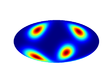
((a)) Target

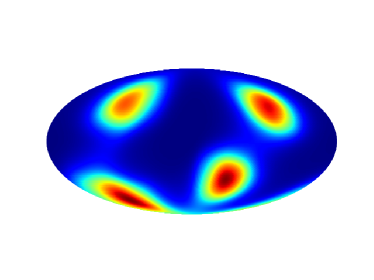
((b)) Model

Figure 7.1: Learned density on $S^{2}$

Manifold	Model	KL[nats]	ESS[%]
$S^{2}$	MS	0.05$\pm$.01	90
	MCNF	0.003$\pm$.001	99.3$\pm$.2
$S^{3}$	MS	0.14	84
	MCNF	0.004$\pm$.001	99.2$\pm$0.2

Table 7.3: Comparing of MCNF and MS flow proposed in Rezende et al., (2020) on a vMF density matching task. Error is computed over 3 replicas of each experiment.

7.2.4 Unitary matrices

The group $U(n):=\{A\in\text{GL}_{n}(\mathbb{C}):A^{\dagger}A=I\}$ is the matrix Lie group formed by all the complex $n\times n$ unitary matrices. Its Lie algebra $\mathfrak{u(n)}=\{A\in\text{M}_{nn}(\mathbb{C})\ |\ A^{\dagger}=-A\}$ is given by the $n\times n$ skew-Hermitian matrices. A basis for $\mathfrak{u(n)}$ is given by the $n^{2}$ matrices:

$$V_{kj}:=E_{kj}-E_{jk}\quad iV_{kj}^{\dagger}:=iE_{kj}+iE_{jk}\quad H_{j}:=iE_{jj}\quad\text{where }1\leq k\!<\!j\leq n$$ (7.13)

where $1\leq k\!<\!j\leq n$ and $i$ denotes is the imaginary unit. For example for $n=2,3$ a basis $\{v_{k}\}_{k=1}^{n^{2}}$ is given by:

$$v_{1,2,3,4}= \begin{bmatrix}0&i\\ i&0\end{bmatrix},\begin{bmatrix}0&1\\ -1&0\end{bmatrix},\begin{bmatrix}i&0\\ 0&0\end{bmatrix},\begin{bmatrix}0&0\\ 0&i\end{bmatrix}.$$ (7.14)

$$v_{1,2,3,4,5,6,7,8,9}:= \begin{bmatrix}0&0&0\\ 0&0&1\\ 0&-1&0\end{bmatrix},\begin{bmatrix}0&0&1\\ 0&0&0\\ -1&0&0\end{bmatrix},\begin{bmatrix}0&1&0\\ -1&0&0\\ 0&0&0\end{bmatrix}\begin{bmatrix}0&0&0\\ 0&0&i\\ 0&i&0\end{bmatrix},$$ (7.15)

$$\begin{bmatrix}0&0&i\\ 0&0&0\\ i&0&0\end{bmatrix},\begin{bmatrix}0&i&0\\ i&0&0\\ 0&0&0\end{bmatrix},\begin{bmatrix}i&0&0\\ 0&0&0\\ 0&0&0\end{bmatrix},\begin{bmatrix}0&0&0\\ 0&i&0\\ 0&0&0\end{bmatrix},\begin{bmatrix}0&0&0\\ 0&0&0\\ 0&0&i\end{bmatrix},$$ (7.16)

We use the generating set $\{v_{k}^{L}\}_{k=1}^{n^{2}}\subset\Gamma^{\infty}\left(U(n),TU(n)\right)$, when parameterizing vector fields on $U(2)$ and $U(3)$ in the experiments.

7.2.5 Special Unitary matrices

The group $SU(n):=\{A\in\text{GL}_{n}(\mathbb{C}):A^{\dagger}A=I,\ \text{det}(U)=1\}$ is the matrix Lie group of complex $n\times n$ unitary matrices with unit determinant. The lie algebra $\mathfrak{su}(n):=\{A\in\text{M}(n,\mathbb{C}):A^{\dagger}=-A,\ \text{tr}(A)=0\}$ is given by the traceless skew-Hermitian matrices. A basis for $\mathfrak{su(n)}$ is given by the $n^{2}-1$ matrices:

$$V_{kj}=E_{kj}-E_{jk}\quad iV_{kj}^{\dagger}=iE_{kj}+iE_{jk}\quad H_{k}=iE_{kk}-iE_{k+1k+1}$$ (7.17)

where $1\leq k\!<\!j\leq n$. When $n=2$ a basis $\{v_{i}\}_{i=1}^{3}$ for $\mathfrak{su}(2)$ is given by Pauli matrices:

$$\quad v_{1,2,3}=\begin{bmatrix}0&i\\ i&0\end{bmatrix},\begin{bmatrix}0&1\\ -1&0\end{bmatrix},\begin{bmatrix}-i&0\\ 0&i\end{bmatrix}.$$ (7.18)

When $n=3$ a basis $\{v_{i}\}_{i=1}^{8}$ for $\mathfrak{su}(3)$ is:

$$v_{1,2,3,4,5,6,7,8}= \begin{bmatrix}0&0&0\\ 0&0&1\\ 0&-1&0\end{bmatrix},\begin{bmatrix}0&0&1\\ 0&0&0\\ -1&0&0\end{bmatrix},\begin{bmatrix}0&1&0\\ -1&0&0\\ 0&0&0\end{bmatrix}\begin{bmatrix}0&0&0\\ 0&0&i\\ 0&i&0\end{bmatrix},$$ (7.19)

$$\begin{bmatrix}0&0&i\\ 0&0&0\\ i&0&0\end{bmatrix},\begin{bmatrix}0&i&0\\ i&0&0\\ 0&0&0\end{bmatrix},\begin{bmatrix}i&0&0\\ 0&-i&0\\ 0&0&0\end{bmatrix},\begin{bmatrix}0&0&0\\ 0&i&0\\ 0&0&-i\end{bmatrix}.$$ (7.20)

Experiments:

The target density used in the experiments for $U(n)$ and $SU(n)$ is a $k=4$ mixture of distributions with components given by:

$$\log\rho(Q|\beta,W)=\frac{\beta}{n}\text{tr}\left(Real\left(W^{\dagger}Q\right)\right)\quad \forall Q\in U(n),SU(n)$$ (7.21)

$$\text{where }W\in U(n),SU(n)$$ (7.22)

As a base density $\mu$, and as a initial probability density, we used the bi-invariant density associated to the Haar measure on $SU(n),U(n)$. The algorithm described in Mezzadri, (2006) was employed for sampling.

In the experiments we fixed $n\in\{2,3\}$,$\beta\in\{5,10\}$ and the centers $W_{i}\in U(n),SU(n)$ were sampled uniformly at random for each run. Results are reported in table 7.4.

Table 7.4: Evaluation of Manifold Continuous Normalizing Flow (MCNF) on $U(n)$ and $SU(n)$. The experiments on the Highlighted rows were repeated 5 times and reported in the summary Table 7.7

Manifold	$\beta$	KL[nats]	ESS[%]
$SU(2)$	5	$0.001$	$99.9$
$SU(2)$	10	$0.005_{\pm 0.003}$	$98.6_{\pm 0.8}$
$SU(3)$	5	$0.003$	$99.3$
$SU(3)$	10	$0.01_{\pm 0.003}$	$97.1_{\pm 0.6}$
$U(2)$	5	$0.003$	$99.3$
$U(2)$	10	$0.02_{\pm 0.008}$	$95.4_{\pm 1.4}$
$U(3)$	5	$0.006$	$98.9$
$U(3)$	10	$0.05_{\pm 0.008}$	$91.5_{\pm 1.3}$

Additional experiment: matching conjugation invariant densities on SU(3)

To further investigate the ability of MCNF to model multimodal densities, we trained a model to match the following conjugation invariant probability density on $SU(3)$:

$$\log\widetilde{\rho}(A|\beta,c)=\frac{\beta}{3}Real\left(\text{tr}\left(\sum_{j=1}^{3}c_{j}U^{j}\right)\right)$$ (7.23)

Where $c=(c_{1},c_{2},c_{3})\in\mathbb{R}^{3}$. Results are reported in Table 7.5. As a reference, we report the scores achieved by the conjugation equivariant flow described in Kanwar et al., (2020). Notice that a throughout comparison of the models might be inappropriate since the permutation equivariant flow already incorporates the symmetries of the target distribution. Thus reducing to modelling a flow on the two-dimensional simplex $\Delta_{2}$. Our model instead parameterizes an unconstrained density on $SU(3)$. Notwithstanding the above a MCNF, can match the performance of the conjugation equivariant flow in all settings, achieving in some cases significantly better results. We interpret these results as additional evidence of the high expressive power of our model.

Table 7.5: ESS of Manifold Continuous Normalizing Flow (MCNF) on conjugation invariant density matching task on $SU(3)$. Results are compared with conjugation equivariant flow (CEF) defined by Kanwar et al., (2020).

Setup	Model	$\beta=1$	$\beta=5$	$\beta=9$
$c=(0.17,-0.65,1.22)$	CEF	97	80	82
	MCNF	98.3	91.2	83.5
$c=(0.98,-0.63,-0.21)$	CEF	99	91	73
	MCNF	99.5	98.5	97.4

7.2.6 Positive definite symmetric matrices

The manifold $\text{Sym}^{+}(n)=\{Q\in\text{M}_{nn}(\mathbb{R})\ |\ Q^{\top}=Q,\ x^{\top}Qx>0\ \forall x\in\mathbb{R}^{n}\}$ is formed by all $n\times n$ symmetric positive definite matrices. $\text{Sym}^{+}(n)$ is a convex cone on the manifold of symmetric matrices $\text{Sym}(n)\cong\mathbb{R}^{\frac{n(n+1)}{2}}$.

$\text{Sym}^{+}(n)$ can be considered a homogeneous $GL(n)$ space with action given by matrix congruence:

$$GL(n)\times\text{Sym}^{+}(n) \to\text{Sym}^{+}(n)$$ (7.24)

$$(A,Q) \mapsto A^{\top}QA$$ (7.25)

By Proposition 5.3.1 the basis $\{E_{kj}\}_{k,j=1}^{n}\subset\mathfrak{gl(n)}$ induces the generating set $\{\widetilde{E}_{kj}\}_{k,j=1}^{n}\subset\Gamma^{\infty}\left(\text{Sym}^{+}(n),T\text{Sym}^{+}(n)\right)$ for the smooth vector fields on $\text{Sym}^{+}(n)$:

$$\widetilde{E}_{kj}(Q) =\dfrac{d}{dt}\biggr{|}_{t=0}\bigg{[}\left(I+E_{jk}t\right)Q\left(I+E_{kj}t\right)+o(t)\bigg{]}=$$ (7.26)

$$=E_{jk}Q+QE_{jk}\in T_{Q}\text{Sym}^{+}(n)\cong\text{Sym}(n)\subset\text{M}_{nn}(\mathbb{R})\quad\forall Q\in\text{Sym}^{+}(n)$$ (7.27)

(where $k,j\in\left[n\right]$), which we will use in the experiments when parameterizing vector fields on $\text{Sym}^{+}(n)$. Notice that we can identify $T_{Q}\text{Sym}^{+}(n)\cong\text{Sym}(n):=\{Q\in\text{M}_{nn}(\mathbb{R})\ |\ Q^{\top}=Q\},\ \forall Q\in\text{Sym}^{+}(n)$.

We can define on $\text{Sym}^{+}(n)$ the following group action invariant Riemannian metric:

$$g_{Q}(A,B)=\text{tr}\left(Q^{-1}AQ^{-1}B\right)$$ (7.28)

The corresponding group invariant volume density $\mu_{g}$ is given by

$$\mu_{g}(Q)=\text{det}(Q)^{-\frac{(n+1)}{2}}\left|\bigwedge_{1\leq k\leq j\leq n}dQ_{kj}\right|\quad\forall Q\in\text{Sym}^{+}(n)$$ (7.29)

Where $\left|\bigwedge_{1\leq k\leq j\leq n}dQ_{kj}\right|$ represents the uniform density associated with the Lebesgue measure on $\mathbb{R}^{\frac{n(n+1)}{2}}$. What discussed in section 5.3 then assures us that the generating set described in Equation (7.26) is formed by vector fields with zero divergence with respect to $\mu_{g}$.

Experiments:

The target density used in the experiments for $\text{Sym}^{+}(n)$ is a $k=4$ mixture of Wishart distributions with components given by:

$$\widetilde{\rho}(Q|\beta,W)\left|\bigwedge_{1\leq k\leq j\leq n}dQ_{kj}\right|=\frac{\det(Q)^{\frac{\beta-n-1}{2}}}{\det(W)^{\frac{\beta}{2}}}\exp\left(-\frac{1}{2}\text{tr}\left(W^{-1}Q\right)\right)\left|\bigwedge_{1\leq k\leq j\leq n}dQ_{kj}\right|$$

$$\forall Q\in\text{Sym}^{+}(n)$$

Where $n+1\leq\beta\in\mathbb{N}$ corresponds to the degrees of freedom, and $W\in\text{Sym}^{+}(n)$. The above probability density function is given with respect to the density associated with the Lebesgue measure in $\mathbb{R}^{\frac{n(n+1)}{2}}$. If we use as a base density the congruence invariant density $\mu_{g}$ defined by Equation (7.29) we can rewrite:

$$\rho(Q|\beta,W)\mu_{g}(Q)=\left(\frac{\det(Q)}{\det(W)}\right)^{\frac{\beta}{2}}\exp\left(-\frac{1}{2}\text{tr}\left(W^{-1}Q\right)\right)\mu_{g}(Q)$$ (7.30)

$$\forall Q\in\text{Sym}^{+}(n)$$ (7.31)

Algorithm 1 in Section 4.4.2 of Camaño-Garcia, (2006) was employed for sampling. As initial probability density, we used $\rho(\cdot|\beta,I\frac{5}{\beta})\mu_{g}$. In the experiments, we fixed $\beta\in\{5,10,20\}$, $n\in\{2,3\}$ with centers:

$$W_{1,2,3,4}:=\frac{1}{\beta}\widehat{W}_{1,2,3,4}\quad\text{where}$$ (7.32)

$$\widehat{W}_{1,2,3,4}:=\begin{bmatrix}1&0\\ 0&2\end{bmatrix},\begin{bmatrix}2&0\\ 0&1\end{bmatrix},\begin{bmatrix}1&1\\ 1&2\end{bmatrix},\begin{bmatrix}2&-1\\ -1&1\end{bmatrix}.$$ (7.33)

$$W_{1,2,3,4}:=\frac{1}{\beta}\widehat{W}_{1,2,3,4}\quad\text{where}$$ (7.34)

$$\widehat{W}_{1,2,3,4}:=\begin{bmatrix}2&0&0\\ 0&1&0\\ 0&0&1\end{bmatrix},\begin{bmatrix}1&0&0\\ 0&2&0\\ 0&0&1\end{bmatrix},\begin{bmatrix}1&0&0\\ 0&1&0\\ 0&0&2\end{bmatrix},\begin{bmatrix}2&0&0\\ 0&2&0\\ 0&0&2\end{bmatrix}.$$ (7.35)

Results are reported in Table 7.6.

Table 7.6: Evaluation of Manifold Continuous Normalizing Flow (MCNF) on $\text{Sym}^{+}(n)$. The experiments on the Highlighted rows were repeated 5 times and reported in the summary Table 7.7

Manifold	$\beta$	KL[nats]	ESS[%]
$\text{Sym}^{+}(3)$	5	$0.006$	$98.9$
$\text{Sym}^{+}(3)$	10	$0.007$	$98.4$
$\text{Sym}^{+}(3)$	20	$0.02$	$94.9$
$\text{Sym}^{+}(2)$	5	$0.001$	$99.7$
$\text{Sym}^{+}(2)$	10	$0.004$	$99.2$
$\text{Sym}^{+}(2)$	20	$0.009_{\pm 0.002}$	$98.01_{\pm 0.1}$

7.3 Summary of results and comment

Table 7.7: Summary of manifold montinuous normalizing flow (MCNF) on mixture density matching task. Error is computed over 5 replicas of each experiment.

Manifold	dimension	KL[nats]	ESS[%]
$\mathcal{V}_{1}(\mathbb{R}^{3})\cong\mathbb{S}^{2}$	2	$0.003_{\pm 0.001}$	$99.3_{\pm 0.8}$
$\mathcal{V}_{1}(\mathbb{R}^{4})\cong\mathbb{S}^{3}$	3	$0.006_{\pm 0.002}$	$98.6_{\pm 0.5}$
$\mathcal{V}_{2}(\mathbb{R}^{4})$	5	$0.02_{\pm 0.006}$	$96.5_{\pm 1.1}$
$\mathcal{V}_{2}(\mathbb{R}^{5})$	7	$0.02_{\pm 0.003}$	$97.1_{\pm 0.6}$
$SO(3)$	3	$0.03_{\pm 0.007}$	$95.3_{\pm 0.8}$
$\mathbb{S}^{10}$	10	$0.01_{\pm 0.003}$	$97.2_{\pm 0.6}$
$\mathbb{S}^{20}$	20	$0.02_{\pm 0.003}$	$95.4_{\pm 0.4}$
$SU(2)$	3	$0.005_{\pm 0.003}$	$98.6_{\pm 0.8}$
$SU(3)$	8	$0.01_{\pm 0.003}$	$97.1_{\pm 0.6}$
$U(2)$	4	$0.02_{\pm 0.008}$	$95.4_{\pm 1.4}$
$U(3)$	9	$0.05_{\pm 0.008}$	$91.5_{\pm 1.3}$
$\text{Sym}^{+}(2)$	3	$0.009_{\pm 0.002}$	$98.01_{\pm 0.1}$

Table 7.7 shows that the proposed MCNF is able to closely match the target densities on all the spaces, with low KL and high ESS ($>90\%$). The results on $\mathbb{S}^{10}$ and $\mathbb{S}^{20}$ show that the proposed method can effectively scale to higher dimensional manifolds. Interestingly, the experiments seem to indicate that the model has more difficulty in matching the target distribution when the space is not simply connected ($SO(3),\ U(2),\ U(3)$).

Chapter 8 Conclusion

In this thesis we presented a universal methodology for building free form normalizing flows on manifolds. To achieve this objective we generalized neural ordinary differential equations based architectures and continuous normalizing flows to arbitrary smooth manifolds. As manifolds are nontrivial mathematical objects to work with, we strove to build our theory on strong mathematical foundations, recognizing in differential geometry the correct language to define our framework.

Working with intrinsically defined objects on manifolds has several advantages over employing quantities that depend on a particular parameterization or defined on local coordinates. First of all, it decouples the mathematical derivation from a specific algorithmic choice, making it easier to use the most convenient parameterization for each specific space. For example, our definition of cotangent lift allows to freely choose the numerical integration method to use in practice. Secondly, our formulation paves the way for future research, such as the design of theoretically sound regularization methods, or the investigation of stability properties and approximation capabilities of neural ODEs on manifolds.

Notwithstanding the above, we strove to present a framework that can be easily implemented and involves efficient computations. We achieve this by employing a generating set of vector fields in combination with free form neural architectures to parameterize vector fields. We then showed that this formulation leads to a simplified divergence calculation for homogeneous spaces and Lie groups, spaces of outstanding importance in many fields of science and engineering. These claims are supported by our experiments, which prove how the defined framework can be used to successfully train normalizing flows on a wide array of spaces. An aspect that we didn’t consider in this thesis, and that we leave for future research, is using specific numerical integrators adapted to the manifold structure.

We hope that the methods and algorithms developed in this thesis will allow probabilistic deep learning models to tackle problems in many scientific disciplines outside machine learning.

Appendix A Densities and induced measure

A.1 volume forms

In the rest of the chapter $M$ will be a smooth manifold of dimension $n$

Definition A.0.1.

A volume form $\omega$ is a section of the line bundle $\Lambda^{n}T^{*}M=\Lambda^{top}T^{*}M$, that is $\omega\in\Gamma\left(M,\Lambda^{n}T^{*}M\right)$.

In any smooth chart $\left(U;x_{i}\right)$ a volume form $\omega$ can be written as:

$$\omega\big{|}_{U}=fdx_{1}\wedge\cdots\wedge dx_{n}\quad\quad f\in C(U)$$ (A.1)

If the manifold is orientable, then there exists a smooth non vanishing volume form that is positively oriented at each point . Since $\Lambda^{n}T^{*}M$ is a vector bundle of rank 1, orientability implies that the line bundle is isomorphic to the trivial bundle $M\times\mathbb{R}$, such that any non vanishing (smooth) volume form is a (smooth) global frame.

This means that fixed a smooth nonvanishing volume form $\omega\in\Gamma^{\infty}\left(M,\Lambda^{n}T^{*}M\right)$ we have a $1$ to $1$ correspondence between continuous (resp. smooth) functions on $M$ and (resp. smooth) volume forms on $M$:

$$C(M) \to\Gamma\left(M,\Lambda^{n}T^{*}M\right)\qquad\text{and}\quad C^{\infty}(M) \to\Gamma^{\infty}\left(M,\Lambda^{n}T^{*}M\right)$$ (A.2)

$$f \mapsto f\omega f \mapsto f\omega$$ (A.3)

The map depends explicitly on the initial choice for $\omega$. On semi-Riemannian manifolds there is a standard choice for this form:

Prop A.0.1.

Suppose $(M,g)$ is an oriented semi Riemannian n-manifold, and $n\geq 1$. There is a unique smooth non vanishing form $\omega_{g}\in\Gamma^{\infty}\left(N,\Lambda^{n}T^{*}M\right)$ , called the semi Riemannian volume form, that satisfies:

$$\omega_{g}(E_{1},\cdots,E_{n})=1$$ (A.4)

for every local oriented orthonormal frame $\{E_{i}\}$ on $M$.

In any local coordinates $\left(U;x_{i}\right)$ the semi Riemannian volume form $\omega_{g}$ can be written as:

$$\omega_{g}\big{|}_{U}=\sqrt{|\det g_{ij}|}\ dx_{1}\wedge\cdots\wedge dx_{n}$$ (A.5)

Where for each point $q\in U$, $g_{ij}(q)$ is the symmetric matrix that gives the local coordinate expression for the metric $g$.

Given a volume form on a smooth manifold we can define its integral. For the rest of the section, we will outline the principal steps of the construction. The interested reader can consult Chapter 16 of Lee, (2013) for a complete exposition.

We first define the integral of a volume form $\omega$ compactly supported on the domain of a smooth chart $(U,\varphi)$ with coordinates $(x_{i})$:

$$\int_{M}\omega=\int_{U}fdx_{1}\wedge\cdots\wedge dx_{n}: =\pm\int_{\varphi(U)}f\circ\varphi^{-1}dx_{1}\wedge\cdots\wedge dx_{n}=$$ (A.6)

$$=\int_{\varphi(U)}f(\varphi^{-1}(x))\textnormal{d}x$$ (A.7)

Where $\omega|_{U}=fdx_{1}\wedge\cdots\wedge dx_{n}$ and the sign depends on the orientation. Notice that $f\circ\varphi^{-1}dx_{1}\wedge\cdots\wedge dx_{n}=(\varphi^{-1})^{*}\omega\in\Lambda^{n}T^{*}\varphi(U)$ is a volume form on a compactly supported open set of $\mathbb{R}^{n}$, and we define its integral as simply "erasing" the wedges and computing the corresponding Riemann integral. . Proposition 16.4 of Lee, (2013) ensures that the integral is well defined, i.e. that it does not depend on the choice of the smooth chart whose domain contains the support of $\omega$.

Once we have defined the integral for a volume form compactly supported in one chart domain, we can define the general integral of a volume form $\omega$.This is done using the partition of unity to express the initial volume form as a sum of volume forms which are compactly supported in one chart domain. To achieve this, we first cover the support of $\omega$ using a finite collection $\{U_{i}\}$ of open smooth chart domains . We then take a partition of unity ${\alpha_{i}}$ subordinate to the open collection. We then define the integral of $\omega$ over $M$ as:

$$\int_{M}\omega:=\sum_{i}\int_{M}\alpha_{i}\omega$$ (A.8)

It can be shown that this definition does not depend on the particular choice of the open cover and partition of unity .

A.2 Densities

Definition A.0.2.

Let $V$ be a $n$-dimensional vector space. A density on a vector space V is a function:

$$\mu:\underbrace{V\times\cdots\times V}_{\text{n times}}\to\mathbb{R}$$ (A.9)

Such that for every linear map $T:V\to V$:

$$\mu(Tv_{1},\cdots,Tv_{n})=|\det T|\mu(v_{1},\cdots,v_{n})\quad\forall v_{1},\cdots,v_{n}\in V$$ (A.10)

A density is said positive if $\mu(v_{1},\cdots,v_{n})>0$, for every linear independent tuple $(v_{i})_{i\in[n]}$. A negative density is similarly defined.

The set of all densities on $V$, $\mathcal{D}(V)$ is a 1 dimensional vector space. Given a n-form $\omega\in\Lambda^{n}(V^{*})$, we can define a density $|\omega|:V\times\cdots\times V\to\mathbb{R}$ as

$$|\omega|(v_{1},\cdots,v_{n})=|\omega(v_{1},\cdots,v_{n})|$$ (A.11)

On a smooth manifold $M$ we can take the collection of all densities defined on each tangent space $T_{q}M,\ q\in M$, and give it a vector bundle structure. More formally, we define the density bundle of $M$ as the set:

$$\mathcal{D}(M):=\bigsqcup_{q\in M}\mathcal{D}(T_{q}M)$$ (A.12)

Moreover if we define $\pi:\mathcal{D}(M)\to M$ to be the natural projection that sends every element of $\mathcal{D}(T_{q}M)$ to $q$ we have:

Prop A.0.2.

$(\mathcal{D}(M),\pi,M)$ with $\mathcal{D}(M)$ and $\pi$ defined as above, is a smooth line bundle over $M$.

A section of $\mathcal{D}M$ is called a density on $M$. Densities are closely connected with volume forms. In fact, a non-vanishing volume form $\omega\in\Lambda^{n}T^{*}M$ determines a positive density $|\omega|$, defined as $|\omega|_{q}:=|\omega_{q}|,\ \forall q\in M$. Moreover in local coordinates $(U;x_{i})$ a density $\mu$ can be expressed as:

$$\mu\big{|}_{U}=f|dx_{1}\wedge\cdots\wedge dx_{n}|\quad f\in C(U)$$ (A.13)

Like differential forms, densities can be pulled back:

Definition A.0.3.

Let $F:M\to N$ be a smooth map between manifolds of dimension $n$, and $\mu$ a desnity over $N$. We define a density $F^{*}\mu$ on $M$, called the pullback density, as:

$$(F^{*}\mu)_{p}(v_{1},\cdots,v_{n})=\mu_{F(p)}(\textnormal{d}F_{p}{v_{1}},\cdots,\textnormal{d}F_{p}{v_{n}})$$ (A.14)

Prop A.0.3.

Let $G:P\to M$ and $F:M\to N$ be smooth maps between $n$ dimensional manifolds, and let $\mu$ be a density on $N$

1. $\forall f\in C^{\infty}(N),F^{*}(f\mu)=(f\circ F)F^{*}\mu$

2. If $\omega$ is an $n$-form on $N$, then $F^{*}|\omega|=|F^{*}\omega|$

3. If $\mu$ is smooth, then $F^{*}\mu$ is a smooth density on $M$

4. $(F\circ G)^{*}\mu=G^{*}(F^{*}\mu)$

Differently from volume forms, a smooth positive density exists on every smooth manifold:

Prop A.0.4.

If $M$ is a smooth manifold, there exists a smooth positive density on $M$

Since the density bundle is a line bundle, the previous proposition implies that the density bundle is always parallelizable and that any positive density forms a global frame. This means that fixed a smooth positive density $\mu\in\Gamma^{\infty}\left(M,\mathcal{D}M\right)$ we have a $1$ to $1$ correspondence between continuous (resp. smooth) functions on $M$ and (resp. smooth) densities on $M$:

$$C(M) \to\Gamma\left(M,\mathcal{D}M\right)\qquad\text{and}\quad C^{\infty}(M) \to\Gamma^{\infty}\left(M,\mathcal{D}M\right)$$ (A.15)

$$f \mapsto f\mu f \mapsto f\mu$$ (A.16)

As with volume forms, these maps explicitly depends on the initial choice for $\mu$. Furthermore, in semi-Riemannian manifolds there is a standard choice for this density that generalizes the semi Riemannian volume form:

Prop A.0.5.

Let $(M,g)$ be a semi Riemannian manifold There is a unique smooth positive density $\mu_{g}$ on $M$, called the semi Riemannian density, with the property that

$$\mu_{g}(E_{1},\cdots,E_{n})=1$$

for any local orthonormal frame $(E_{i})$.

On an oriented semi Riemannian manifold we have $\mu_{g}=|\omega_{g}|$.

We can define the integral of compactly supported densities on a manifold. The construction closely mirrors the definition of the integral of volume forms, first defining the integral for densities compactly supported on a chart domain and then generalizing to arbitrary compact support using a partition of unity. For a detailed description of the process, we refer to Lee, (2013). The following proposition illustrates the properties of the integral:

Prop A.0.6.

Suppose M is a n-manifolds and $\mu$,$\eta$ are compactly supported densities on M:

1. linearity If $a,b\in\mathbb{R}$, then:

   $$\int_{M}a\mu+b\eta=a\int_{M}\mu+b\int_{M}\eta.$$ (A.17)

2. positivity If $\mu$ is a positive density, then:

   $$\int_{M}\mu>0$$ (A.18)

This properties fundamentally tell us that this integral is a positive linear functional on the vector space of densities with compact support on a smooth manifold.

A.2.1 Induced measure

Using the correspondence given by Equation (A.15) every nonnegative density defines a positive linear functional on $C_{c}(M)$. In fact, fixed $\mu\in\Gamma\left(M,\mathcal{D}M\right)$ nonnegative density we define:

$$L_{\mu}:C_{c}(M) \to\mathbb{R}$$ (A.19)

$$f \mapsto\int_{M}f\mu$$ (A.20)

We can then use the Riesz representation theorem to (uniquely) define a Radon measure on $M$:

Theorem A.1.

Let $\mathcal{X}$ be a locally compact Hausdorff space, and let $L$ be a positive linear functional on $C_{c}(\mathcal{X})$. Then there exists a unique Radon measure $\mu$ such that:

$$Lf=\int_{\mathcal{X}}fd\mu,\quad\forall f\in C_{c}(M)$$ (A.21)

The Radon measure is said to represent the functional $L$.

One direct consequence of the Riesz representation theorem is that if we have two Radon measures $\mu_{1}$ and $\mu_{2}$ on a locally compact Hausdorff space such that their Lebesgue integral coincides on continuous and compactly supported functions:

$$\int_{\mathcal{X}}gd\mu_{1}=\int_{\mathcal{X}}gd\mu_{2}\quad\forall g\in C_{c}(\mathcal{X})$$ (A.22)

then the two measures coincide ($\mu_{1}=\mu_{2}$).

We can use a positive smooth density and the Riesz representation theorem to define a Radon measure on a smooth manifold.

Theorem A.2.

Let $M$ be a smooth manifold and $\mu$ a non negative density on $M$, then there exists a unique Radon regular measure $\tilde{\mu}$ such that:

$$\int_{M}f\mu=\int_{M}fd\tilde{\mu}\quad\forall f\in C_{c}(M)$$ (A.23)

We will say that the measure $\tilde{\mu}$ is derived from $\mu$.

Proof.

We first show that we can apply the Riesz representation theorem for the functional $L_{\mu}$. Since any manifold is a locally compact Hausdorff space, this reduces to proving that $L_{\mu}$ is a positive linear functional. Using Proposition A.0.6 we see that:

$$L_{\mu}(\alpha f+\beta g)=\int_{M}\alpha f\mu+\beta g\mu=\alpha\int_{M}f\mu+\beta\int_{M}g\mu=\alpha L_{\mu}f+\beta L_{\mu}g$$

$$\forall f,g\in C_{c}(M),\ \forall\alpha,\beta\in\mathbb{R}$$

and

$$L_{\mu}f=\int_{M}f\mu\geq 0\quad\forall f\in C_{c}(M),\ f\geq 0$$

This shows that $L_{\mu}$ is a linear positive functional on $C_{c}(M)$, therefore a Radon measure $\tilde{\mu}$ that represents $L_{\mu}$ exists. For Corollary 7.6 in Folland, (1999) any Radon measure in a $\sigma$-compact space is regular. Therefore, since any Manifold is $\sigma$-compact, $\tilde{\mu}$ is also regular. ∎

This choice of measure on $M$ depends on the initial choice for $\mu$. The next proposition shows how two measures derived from two different densities relate to each other:

Prop A.2.1.

Let $\tilde{\eta}$ and $\tilde{\mu}$ two regular Radon measures derived from two densities $\eta$, $\mu$, with $\mu$ positive. Then $\tilde{\nu}\ll\tilde{\mu}$, that is there exists a continuous function $f$ such that $f\tilde{\mu}=\tilde{g}$. If both $\eta$ and $\mu$ are smooth then $f$ is a smooth function.

Proof.

Since every positive density forms a frame for the line bundle $\mathcal{D}M$, we can use Equation (A.15) to state that there exists $f\in C(M)$ such that $\eta=f\mu$. If $\mu$ and $\eta$ are both smooth then also $f$ is smooth.

Consider now the measure $f\tilde{\mu}$, we see that $\tilde{\eta}$ and $f\tilde{\mu}$ represent the same positive linear functional on $C_{c}(M)$:

$$\int_{M}gd\tilde{\eta}=\int_{M}g\eta=\int_{M}gf\mu=\int_{M}gd(f\tilde{\mu})$$ (A.24)

If $f\tilde{\mu}$ is a Radon measure then by Riesz representation theorem we can conclude that the two measures coincide.

To show that $f\tilde{\mu}$ is Radon we can use Theorem 7.8 from Folland, (1999), that tells us that a in a locally compact space in which every open set is $\sigma$ compact, every Borel measure on $\mathcal{X}$ which is finite on compact sets is Radon. Since by definition every manifold satisfies the topological requirements that the space needs to satisfy, we are left to prove that $f\tilde{\mu}$ is finite on compact sets. Then, fixed $K\subseteq M$ compact, we have:

$$[f\tilde{\mu}](K)=\int_{K}fd\tilde{\mu}\leq\sup_{K}(f)\int d\tilde{\mu}=\sup_{K}(f)\tilde{\mu}(K)<+\infty$$ (A.25)

Where in the last equality we have used that, since $\tilde{\mu}$ is Radon, $\tilde{\mu}(K)<+\infty$, and that $\sup_{K}(f)<+\infty$ since $f$ is continuous and $K$ compact. Therefore $f\tilde{\mu}$ is finite on compact sets and this concludes our proof. ∎

In practice, fixed a smooth positive density $\mu$, we will work with absolutely continuous probability measures $g\tilde{\mu}$, where $g\in L^{1}_{\tilde{\mu}}(M),\ g\geq 0,\ \int_{M}gd\tilde{\mu}=1$. Then Proposition (A.2.1) tells us that that the set of measures that we can express in this way does not depend on the initial choice for $\mu$.

Glossary

Acronyms

References

• Agrachev et al., (2019) Agrachev, A., Barilari, D., and Boscain, U. (2019). A comprehensive introduction to sub-riemannian geometry.
• Agrachev and Sachkov, (2013) Agrachev, A. A. and Sachkov, Y. (2013). Control theory from the geometric viewpoint, volume 87. Springer Science & Business Media.
• Alekseevsky et al., (1994) Alekseevsky, D., Grabowski, J., Marmo, G., and Michor, P. W. (1994). Poisson structures on the cotangent bundle of a lie group or a principle bundle and their reductions. Journal of Mathematical Physics, 35(9):4909–4927.
• Ayala et al., (2009) Ayala, V., Rodríguez, J., and Sanmartin, L. (2009). Optimality on homogeneous spaces, and the angle system associated with a bilinear control system. SIAM J. Control and Optimization, 48:2636–2650.
• Bates, (2014) Bates, J. (2014). The embedding dimension of laplacian eigenfunction maps. Applied and Computational Harmonic Analysis, 37(3):516–530.
• Bose et al., (2020) Bose, A. J., Smofsky, A., Liao, R., Panangaden, P., and Hamilton, W. L. (2020). Latent variable modelling with hyperbolic normalizing flows. arXiv preprint arXiv:2002.06336.
• Boyda et al., (2020) Boyda, D., Kanwar, G., Racanière, S., Rezende, D. J., Albergo, M. S., Cranmer, K., Hackett, D. C., and Shanahan, P. E. (2020). Sampling using $su(n)$ gauge equivariant flows.
• Bradbury et al., (2018) Bradbury, J., Frostig, R., Hawkins, P., Johnson, M. J., Leary, C., Maclaurin, D., and Wanderman-Milne, S. (2018). JAX: composable transformations of Python+NumPy programs.
• Camaño-Garcia, (2006) Camaño-Garcia, G. (2006). Statistics on Stiefel manifolds. PhD thesis, Iowa State University.
• Cao and Aziz, (2020) Cao, N. D. and Aziz, W. (2020). The power spherical distribution. ICML workshop on Invertible Neural Networks, Normalizing Flows, and Explicit Likelihood Models.
• Chen and Verstraelen, (2013) Chen, B.-Y. and Verstraelen, L. (2013). Laplace transformations of submanifolds.
• Chen et al., (2018) Chen, R. T. Q., Rubanova, Y., Bettencourt, J., and Duvenaud, D. K. (2018). Neural ordinary differential equations. In Bengio, S., Wallach, H., Larochelle, H., Grauman, K., Cesa-Bianchi, N., and Garnett, R., editors, Advances in Neural Information Processing Systems 31, pages 6571–6583. Curran Associates, Inc.
• Da Silva, (2001) Da Silva, A. C. (2001). Lectures on symplectic geometry, volume 3575. Springer.
• Davidson et al., (2018) Davidson, T. R., Falorsi, L., De Cao, N., Kipf, T., and Tomczak, J. M. (2018). Hyperspherical variational auto-encoders. 34th Conference on Uncertainty in Artificial Intelligence (UAI-18).
• Davidson et al., (2019) Davidson, T. R., Tomczak, J. M., and Gavves, E. (2019). Increasing expressivity of a hyperspherical vae. NeurIPS, in Workshop on Bayesian Deep Learning.
• Dinh et al., (2015) Dinh, L., Krueger, D., and Bengio, Y. (2015). Nice: Non-linear independent components estimation. ICLR Workshop.
• Falorsi et al., (2018) Falorsi, L., de Haan, P., Davidson, T. R., De Cao, N., Weiler, M., Forré, P., and Cohen, T. S. (2018). Explorations in homeomorphic variational auto-encoding. ICML workshop on Theoretical Foundations and Applications of Deep Generative Models.
• Falorsi et al., (2019) Falorsi, L., de Haan, P., Davidson, T. R., and Forré, P. (2019). Reparameterizing distributions on lie groups. AISTATS.
• Figurnov et al., (2018) Figurnov, M., Mohamed, S., and Mnih, A. (2018). Implicit reparameterization gradients. In Advances in Neural Information Processing Systems, pages 441–452.
• Folland, (1999) Folland, G. (1999). Real analysis: modern techniques and their applications. Pure and applied mathematics. Wiley.
• Gemici et al., (2016) Gemici, M. C., Rezende, D., and Mohamed, S. (2016). Normalizing flows on riemannian manifolds. arXiv preprint arXiv:1611.02304.
• Grathwohl et al., (2019) Grathwohl, W., Chen, R. T. Q., Bettencourt, J., and Duvenaud, D. (2019). Scalable reversible generative models with free-form continuous dynamics. In International Conference on Learning Representations.
• Haber and Ruthotto, (2017) Haber, E. and Ruthotto, L. (2017). Stable architectures for deep neural networks. Inverse Problems, 34(1):014004.
• Hairer et al., (2006) Hairer, E., Lubich, C., and Wanner, G. (2006). Geometric numerical integration. Structure-preserving algorithms for ordinary differential equations. 2nd ed, volume 31. Springer Science & Business Media.
• Howard, (1994) Howard, R. (1994). Analysis on homogeneous spaces.
• Hutchinson, (1989) Hutchinson, M. (1989). A stochastic estimator of the trace of the influence matrix for laplacian smoothing splines. Communication in Statistics- Simulation and Computation, 18:1059–1076.
• Kanwar et al., (2020) Kanwar, G., Albergo, M. S., Boyda, D., Cranmer, K., Hackett, D. C., Racanière, S., Rezende, D. J., and Shanahan, P. E. (2020). Equivariant flow-based sampling for lattice gauge theory. arXiv preprint arXiv:2003.06413.
• Kingma and Ba, (2015) Kingma, D. P. and Ba, J. (2015). Adam: A method for stochastic optimization. International Conference on Learning Representations.
• Kingma and Welling, (2014) Kingma, D. P. and Welling, M. (2014). Auto-encoding variational bayes. Proceedings of the 2nd International Conference on Learning Representations (ICLR).
• Kish, (1965) Kish, L. (1965). Survey sampling. American Political Science Review, 59(4):1025–1025.
• Kobyzev et al., (2020) Kobyzev, I., Prince, S., and Brubaker, M. (2020). Normalizing flows: An introduction and review of current methods. IEEE Transactions on Pattern Analysis and Machine Intelligence.
• Kunzinger et al., (2006) Kunzinger, M., Schichl, H., Steinbauer, R., and Vickers, J. A. (2006). Global gronwall estimates for integral curves on riemannian manifolds. Revista Matemática Complutense, 19(1):133–137.
• Lee, (2006) Lee, J. M. (2006). Riemannian manifolds: an introduction to curvature, volume 176. Springer Science & Business Media.
• Lee, (2013) Lee, J. M. (2013). Smooth manifolds. In Introduction to Smooth Manifolds, pages 1–31. Springer.
• Lou et al., (2020) Lou, A., Lim, D., Katsman, I., Huang, L., Jiang, Q., Lim, S.-N., and Sa, C. D. (2020). Neural manifold ordinary differential equations.
• Mathieu et al., (2019) Mathieu, E., Le Lan, C., Maddison, C. J., Tomioka, R., and Teh, Y. W. (2019). Continuous hierarchical representations with poincaré variational auto-encoders. In Advances in neural information processing systems, pages 12544–12555.
• Mathieu and Nickel, (2020) Mathieu, E. and Nickel, M. (2020). Riemannian continuous normalizing flows.
• Mezzadri, (2006) Mezzadri, F. (2006). How to generate random matrices from the classical compact groups. Notices of the American Mathematical Society, 54.
• Moakher and Zerai, (2011) Moakher, M. and Zerai, M. (2011). The riemannian geometry of the space of positive-definite matrices and its application to the regularization of positive-definite matrix-valued data. Journal of Mathematical Imaging and Vision, 40:171–187.
• Mohamed et al., (2020) Mohamed, S., Rosca, M., Figurnov, M., and Mnih, A. (2020). Monte carlo gradient estimation in machine learning. Journal of Machine Learning Research, 21(132):1–62.
• Naesseth et al., (2017) Naesseth, C., Ruiz, F., Linderman, S., and Blei, D. (2017). Reparameterization gradients through acceptance-rejection sampling algorithms. In Artificial Intelligence and Statistics, pages 489–498.
• Nagano et al., (2019) Nagano, Y., Yamaguchi, S., Fujita, Y., and Koyama, M. (2019). A wrapped normal distribution on hyperbolic space for gradient-based learning. In International Conference on Machine Learning, pages 4693–4702.
• Noé et al., (2019) Noé, F., Olsson, S., Köhler, J., and Wu, H. (2019). Boltzmann generators: Sampling equilibrium states of many-body systems with deep learning. Science, 365(6457):eaaw1147.
• O’Neill, (1983) O’Neill, B. (1983). Semi-Riemannian Geometry With Applications to Relativity. Pure and Applied Mathematics. Elsevier Science.
• Papamakarios et al., (2019) Papamakarios, G., Nalisnick, E., Rezende, D. J., Mohamed, S., and Lakshminarayanan, B. (2019). Normalizing flows for probabilistic modeling and inference. stat, 1050:5.
• Pontryagin et al., (1962) Pontryagin, L. S., Mishchenko, E., Boltyanskii, V., and Gamkrelidze, R. (1962). The mathematical theory of optimal processes. Wiley.
• Pérez Rey et al., (2019) Pérez Rey, L. A., Menkovski, V., and Portegies, J. W. (2019). Diffusion variational autoencoders. arXiv.
• Rezende and Mohamed, (2015) Rezende, D. and Mohamed, S. (2015). Variational inference with normalizing flows. In International Conference on Machine Learning, pages 1530–1538.
• Rezende et al., (2020) Rezende, D. J., Papamakarios, G., Racanière, S., Albergo, M. S., Kanwar, G., Shanahan, P. E., and Cranmer, K. (2020). Normalizing flows on tori and spheres. arXiv preprint arXiv:2002.02428.
• Rudin, (1987) Rudin, W. (1987). Real and Complex Analysis, 3rd Ed. McGraw-Hill, Inc., New York, NY, USA.
• Tabak and Turner, (2013) Tabak, E. G. and Turner, C. V. (2013). A family of nonparametric density estimation algorithms. Communications on Pure and Applied Mathematics, 66(2):145–164.
• Tabak et al., (2010) Tabak, E. G., Vanden-Eijnden, E., et al. (2010). Density estimation by dual ascent of the log-likelihood. Communications in Mathematical Sciences, 8(1):217–233.
• Teschl, (1998) Teschl, G. (1998). Topics in real and functional analysis.
• Walschap, (2004) Walschap, G. (2004). Metric Structures in Differential Geometry. Graduate Texts in Mathematics. Springer, softcover reprint of hardcover 1st ed. 2004 edition.
• Wirnsberger et al., (2020) Wirnsberger, P., Ballard, A. J., Papamakarios, G., Abercrombie, S., Racanière, S., Pritzel, A., Rezende, D. J., and Blundell, C. (2020). Targeted free energy estimation via learned mappings. arXiv preprint arXiv:2002.04913.