A Riemannian Newton Trust-Region Method for Fitting Gaussian Mixture Models

Abstract

Gaussian Mixture Models are a powerful tool in Data Science and Statistics that are mainly used for clustering and density approximation. The task of estimating the model parameters is in practice often solved by the Expectation Maximization (EM) algorithm which has its benefits in its simplicity and low per-iteration costs. However, the EM converges slowly if there is a large share of hidden information or overlapping clusters. Recent advances in manifold optimization for Gaussian Mixture Models have gained increasing interest. We introduce an explicit formula for the Riemannian Hessian for Gaussian Mixture Models. On top, we propose a new Riemannian Newton Trust-Region method which outperforms current approaches both in terms of runtime and number of iterations. We apply our method on clustering problems and density approximation tasks. Our method is very powerful for data with a large share of hidden information compared to existing methods.

Keywords— Gaussian mixture models, clustering, manifold optimization, trust-region methods

1 Introduction

Gaussian Mixture Models are widely recognized in Data Science and Statistics. The fact that any probability density can be approximated by a Gaussian Mixture Model with a sufficient number of components makes it an attractive tool in statistics. However, this comes with some computational limitations, where some of them are described in Ormoneit and Tresp (1995), Lee and Mclachlan (2013), Coretto (2021). Nevertheless, we here focus on the benefits of Gaussian mixture models. Besides the goal of density approximation, the possibility of modeling latent features by the underlying components make it also a strong tool for soft clustering tasks. Typical applications are to be found in the area of image analysis (Alfò et al., 2008, Dresvyanskiy et al., 2020, Zoran and Weiss, 2012), pattern recognition (Wu et al., 2012, Bishop, 2006), econometrics (Articus and Burgard, 2014, Compiani and Kitamura, 2016) and many others.

We state the Gaussian Mixture Model in the following:
Let $K\in\mathbb{N}$ be given. The Gaussian Mixture Model (with $K$ components) is given by the (multivariate) density function $p$ of the form

$$p(x)=\sum\limits_{j=1}^{K}\alpha_{j}p_{\mathcal{N}}(x;\mu_{j},\Sigma_{j}),\qquad x\in\mathbb{R}^{d},$$ (1)

with positive mixture components $\alpha_{j}$ that sum up to $1$ and Gaussian density functions $p_{\mathcal{N}}$ with means $\mu_{j}\in\mathbb{R}^{d}$ and covariance matrices $\Sigma_{j}\in\mathbb{R}^{d\times d}$. In order to have a well-defined expression, we impose $\Sigma_{j}\succ 0$, i.e. the $\Sigma_{j}$ are symmetric positive definite.

Given observations $x_{1},\dots,x_{m}$, the goal of parameter estimation for Gaussian Mixture Models consists in maximizing the log-likelihood. This yields the optimization problem

$$\max_{\begin{subarray}{c}{\alpha}\in\Delta_{K}\\ \mu_{j}\in\mathbb{R}^{d}\\ \Sigma_{j}\succ 0\end{subarray}}\sum\limits_{i=1}^{m}\log\left(\sum\limits_{j=1}^{K}\alpha_{j}p_{\mathcal{N}}(x_{i};\mu_{j},\Sigma_{j})\right),$$ (2)

where

$$\Delta_{K}=\{(\alpha_{1},\dots,\alpha_{K}),\text{ }\alpha_{j}\in\mathbb{R}^{+}\forall j,\quad\sum\limits_{j=1}^{K}\alpha_{j}=1\}$$

is the K-dimensional probability simplex and the covariance matrices $\Sigma_{j}$ are restricted to the set of positive definite matrices.

In practice, this problem is commonly solved by the Expectation Maximization (EM) algorithm. It is known that the Expectation Maximization algorithm converges fast if the $K$ clusters are well separated. Ma et al. (2000) showed that in such a case, the convergence rate is superlinear. However, Expectation Maximization has its speed limits for highly overlapping clusters, where the latent variables have a non-neglibible large probability among more than one cluster. In such a case, the convergence is linear (Xu and Jordan, 1996) which might results in slow parameter estimation despite very low per-iteration costs.

From a nonlinear optimization perspective, the problem in (2) can be seen as a constrained nonlinear optimization problem. However, the positive definiteness constraint of the covariance matrices $\Sigma_{j}$ is a challenge for applying standard nonlinear optimization algorithms. While this constraint is naturally fulfilled in the EM algorithm, we cannot simply drop it as we might leave the parameter space in alternative methods. Approaches to this problem like introducing a Cholesky decomposition (Salakhutdinov et al., 2003, Xu and Jordan, 1996), or using interior point methods via smooth convex inequalities (Vanderbei and Benson, 1999) can be applied and one might hope for faster convergence with Newton-type algorithms. Methods like using a Conjugate Gradient Algorithm (or a combination of both EM and CG) led to faster convergence for highly overlapping clusters (Salakhutdinov et al., 2003). However, this induces an additional numeric overhead by imposing the positive-definiteness constraint by a Cholesky decomposition.

In recent approaches Hosseini and Sra (2015, 2020) suggest to exploit the geometric structure of the set of positive definite matrices. As an open set in the set of symmetric matrices, it admits a manifold structure (Bhatia, 2007) and thus the concepts of Riemannian optimization can be applied. The concept of Riemannian optimization, i.e. optimizing over parameters that live on a smooth manifold is well studied and has gained increasing interest in the domain of Data Science, for example for tensor completion problems (Heidel and Schulz, 2018). However, the idea is quite new for Gaussian Mixture Models and Hosseini and Sra (2015, 2020) showed promising results with a Riemannian LBFGS and Riemannian Stochastic Gradient Descent Algorithm. The results in Hosseini and Sra (2015, 2020) are based on a reformulation of the log-likelihood in (2) that turns out to be very efficient in terms of runtime. By design, the algorithms investigated in Hosseini and Sra (2015, 2020) do not use exact second-order information of the objective function. Driven by the quadratic local convergence of the Riemannian Newton method, we thus might hope for faster algorithms with the availability of the Riemannian Hessian. In the present work, we derive a formula for the Riemannian Hessian of the reformulated log-likelihood and suggest a Riemannian Newton Trust-Region method for parameter estimation of Gaussian Mixture Models.

The paper is organized as follows. In Section 2, we introduce the reader to the concepts of Riemannian optimization and the Riemannian setting of the reformulated log-likelihood for Gaussian Mixture Models. In particular, we derive the expression for the Riemannian Hessian in Subsection 2.3 which is a big contribution to richer Riemannian methods for Gaussian Mixture Models. In Section 3 we present the Riemannian Newton Trust-Region Method and prove the global convergence and superlinear local convergence for our problem. We compare our proposed method with existing algorithms both on artificial and real world data sets in Section 4 for the task of clustering and density approximation.

2 Riemannian Setting for Gaussian Mixture Models

We will build the foundations of Riemannian Optimization in the following to specify the characteristics for Gaussian Mixture Models afterwards. In particular, we introduce a formula for the Riemannian Hessian for the reformulated problem which is the basis for second-order optimization algorithms.

2.1 Riemannian Optimization

To construct Riemannian Optimization methods, we briefly state the main concepts of Optimization on Manifolds or Riemannian Optimization. A good introduction is Absil et al. (2008) and Boumal (2020), we here follow the notations of Absil et al. (2008). The concepts of Riemannian Optimization are based on concepts from unconstrained Euclidean optimization algorithms and are generalized to (possibly nonlinear) manifolds.

A manifold is a space that locally resembles Euclidean space, meaning that we can locally map points on manifolds to $\mathbb{R}^{n}$ via bicontinuous mappings. Here, $n$ denotes the dimension of the manifold. In order to define a generalization of differentials, Riemannian optimization methods require smooth manifolds meaning that the transition mappings are smooth functions. As manifolds are in general not vector spaces, standard optimization algorithms like line-search methods cannot be directly applied as the iterates might leave the admissible set. Instead, one moves along tangent vectors in tangent spaces $T_{\theta}{\mathcal{M}}$, local approximations of a point $\theta$ on the manifold, i.e. $\theta\in{\mathcal{M}}$. Tangent spaces are basically first-order approximations of the manifold at specific points and the tangent bundle $T{\mathcal{M}}$ is the disjoint union of the tangent spaces $T_{\theta}{\mathcal{M}}$. In Riemannian manifolds, each of the tangent spaces $T_{\theta}{\mathcal{M}}$ for $\theta\in{\mathcal{M}}$ is endowed with an inner product $\langle\cdot,\cdot\rangle_{\theta}$ that varies smoothly with $\theta$. The inner product is essential for Riemannian optimization methods as it admits some notion of length associated with the manifold. The optimization methods also require some local pull-back from the tangent spaces $T_{\theta}{\mathcal{M}}$ to the manifold ${\mathcal{M}}$ which can be interpreted as moving along a specific curve on ${\mathcal{M}}$ (dotted curve in Figure 2.1). This is realized by the concept of retractions: Retractions are mappings from the tangent bundle $T{\mathcal{M}}$ to the manifold ${\mathcal{M}}$ with rigidity conditions: we move through the zero element $0_{\theta}$ with velocity $\xi_{\theta}\in T_{\theta}{\mathcal{M}}$ , i.e. $DR_{\theta}(0_{\theta})[\xi_{\theta}]=\xi_{\theta}.$ Furthermore, the retraction of $0_{\theta}\in T_{\theta}{\mathcal{M}}$ at $\theta$ is $\theta$ itself (see Figure 2.1).

Roughly spoken, a step of a Riemannian optimization algorithm works as follows:

• At iterate $\theta^{t}$, take a new step $\xi_{\theta^{t}}$ on the tangent space $T_{\theta^{t}}{\mathcal{M}}$

• Pull back the new step to the manifold by applying the retraction at point $\theta^{t}$ by setting $\theta^{t+1}=R_{\theta^{t}}(\xi_{\theta^{t}})$

Here, the crucial part that has an impact on convergence speed is updating the new iterate on the tangent space, just like in the Euclidean case. As Riemannian optimization algorithms are a generalization of Euclidean unconstrained optimization algorithms, we thus introduce a generalization of the gradient and the Hessian.

Figure 2.1: Retraction-based Riemannian Optimization

Riemannian Gradient.

In order to characterize Riemannian gradients, we need a notion of differential of functions defined on manifolds.

The differential of $f:{\mathcal{M}}\rightarrow\mathbb{R}$ at $\theta$ is the linear operator $\text{D}f(\theta):T{\mathcal{M}}_{\theta}\rightarrow\mathbb{R}$ defined by:

$$\text{D}f(\theta)[v]=\frac{d}{dt}f(c(t))\biggr{\rvert}_{t=0},$$

where $c:I\rightarrow{\mathcal{M}}$, $0\in I\subset\mathbb{R}$ is a smooth curve on ${\mathcal{M}}$ with $c^{\prime}(0)=v$.

The Riemannian gradient can be uniquely characterized by the differential of the function $f$ and the inner product associated with the manifold:

The Riemannian gradient of a smooth function $f:M\rightarrow\mathbb{R}$ on a Riemannian manifold is a mapping $\operatorname{grad}f:{\mathcal{M}}\rightarrow T{\mathcal{M}}$ such that, for all $\theta\in{\mathcal{M}}$, $\operatorname{grad}f(\theta)$ is the unique tangent vector in $T_{\theta}{\mathcal{M}}$ satisfying

$$\langle\operatorname{grad}f(\theta),\xi_{\theta}\rangle_{\theta}=\text{D}f(\theta)[\xi_{\theta}]\quad\forall\xi_{\theta}\in{\mathcal{M}}.$$

Riemannian Hessian.

We can also generalize the Hessian to its Riemannian version. To do this, we need a tool to differentiate along tangent spaces, namely the Riemannian connection (for details see (Absil et al., 2008, Section 5.3)).

The Riemannian Hessian of $f:{\mathcal{M}}\rightarrow\mathbb{R}$ at $\theta$ is the linear operator $\operatorname{Hess}f(\theta):T_{\theta}{\mathcal{M}}\rightarrow T_{\theta}{\mathcal{M}}$ defined by

$$\operatorname{Hess}f(\theta)[\xi_{\theta}]=\nabla_{\xi_{\theta}}\operatorname{grad}f(\theta),$$

where $\nabla$ is the Riemannian connection with respect to the Riemannian manifold.

2.2 Reformulation of the Log-likelihood

In Hosseini and Sra (2015), the authors experimentally showed that applying the concepts of Riemannian optimization to the objective in (2) cannot compete with Expectation Maximization. This can be mainly led back to the fact that the maximization in the M-step of EM, i.e. the maximization of the log-likelihood for a single Gaussian, is a concave problem and easy to solve, it even admits a closed-form solution. Nevertheless, when considering Riemannian optimization for (2), the maximization of the log-likelihood of a single Gaussian is not geodesically concave (concavity along the shortest curve connecting two points on a manifold). The following reformulation introduced by Hosseini and Sra (2015) removes this geometric mismatch and results in a speed-up for the Riemannian algorithms.

We augment the observations $x_{i}$ by introducing the observations $y_{i}=(x_{i},1)^{T}\in\mathbb{R}^{d+1}$ for $i=1,\dots,m$ and consider the optimization problem

$$\max_{\theta=((S_{1},\dots,S_{K}),(\eta_{1},\dots,\eta_{K-1}))}\hat{\mathcal{L}}(\theta)=\sum\limits_{i=1}^{m}\log\left(\sum\limits_{j=1}^{K}h^{i}(\theta_{j})\right),$$ (3)

where

$$h^{i}(\theta_{j}) =\frac{\exp(\eta_{j})}{\sum\limits_{k=1}^{K}\exp(\eta_{k})}\frac{\exp\left(\frac{1}{2}\left(1-y_{i}^{T}S_{j}^{-1}y_{i}\right)\right)}{\sqrt{(2\pi)^{d}\det(S_{j})}}=\frac{\exp(\eta_{j})}{\sum\limits_{k=1}^{K}\exp(\eta_{j})}q_{\mathcal{N}}(y_{i};S_{j}),$$ (4)

with $q_{\mathcal{N}}(y_{i};S_{j})=\sqrt{2\pi}\exp(\frac{1}{2})p_{\mathcal{N}}(y_{i};0,S_{j})$ for parameters ${\theta_{j}=(S_{j},\eta_{j})}$, $j=1,\dots,K-1$ and ${\theta_{K}=(S_{K},0)}$.

This means that instead of considering Gaussians of $d$ -dimensional variables $x$, we now consider Gaussians of $d+1$ -dimensional variables $y$ with zero mean and covariance matrices $S_{j}$. The reformulation leads to faster Riemannian algorithms, as it has been shown in Hosseini and Sra (2015) that the maximization of a single Gaussian

$$\max_{S\succ 0}\sum\limits_{i=1}^{m}\log q_{\mathcal{N}}(y_{i};S)$$

is geodesically concave.

Furthermore, this reformulation is faithful, as the original problem (2) and the reformulated problem (3) are equivalent in the followings sense:

Theorem 1

(Hosseini and Sra, 2015, Theorem 2.2) A local maximum of the reformulated GMM log-likelihood $\hat{\mathcal{L}}(\theta)$ with maximizer $\theta^{*}=({\theta}_{1}^{*},\dots,{\theta}_{K}^{*})$, ${\theta}_{j}^{*}=({S}_{j}^{*},{\eta}_{j}^{*})$ is a local maximum of the original log-likelihood $\mathcal{L}((\alpha_{j},\mu_{j},\Sigma_{j})_{j})$ with maximizer $({\alpha}_{j}^{*},{\mu}_{j}^{*},{\Sigma}_{j}^{*})_{j}$. Here, $\mathcal{L}$ denotes the objective in the problem (2).

The relationship of the maximizers is given by

$$S_{j}^{*} =\left(\begin{array}[]{cc}\Sigma_{j}^{*}+\mu_{j}^{*}{\mu_{j}^{*}}^{T}&\quad\mu_{j}^{*}\\ {\mu_{j}^{*}}^{T}&\quad 1\\ \end{array}\right),$$ (7)

$$\eta_{j}^{*} =\log\left(\frac{\alpha_{j}^{*}}{\alpha_{K}^{*}}\right)\quad j=1,\dots,K-1;\quad\eta_{K}\equiv 0.$$ (8)

This means that instead of solving the original optimization problem (2) we can easily solve the reformulated problem (3) on its according parameter space and transform the optima back by the relationships (7) and (8).

Penalizing the objective.

When applying Riemannian optimization algorithms on the reformulated problem (3), covariance singularity is a challenge. Although this is not observed in many cases in practice, it might result in unstable algorithms. This is due to the fact that the objective in (3) is unbounded from above, see Appendix A for details. The same problem is extensively studied for the original problem (2) and makes convergence theory hard to investigate. An alternative consists in considering the maximum a posterior log-likelihood for the objective. If conjugate priors are used for the variables $\mu_{j},\Sigma_{j}$, the optimization problem remains structurally unchanged and results in a bounded objective (see Snoussi and Mohammad-Djafari (2002)). Adapted versions of Expectation Maximization have been proposed in the literature and are often applied in practice.

A similar approach has been proposed in Hosseini and Sra (2020) where the reformulated objective (3) is penalized by an additive term that consists of the logarithm of the Wishart prior, i.e. we penalize each of the $K$ components with

$$\psi(S_{j},\Psi)=-\frac{\rho}{2}\log\det(S_{j})-\frac{\beta}{2}\text{tr}(\Psi{S_{j}}^{-1}),$$ (9)

where $\Psi$ is the block matrix

$$\Psi=\left(\begin{array}[]{cc}\frac{\gamma}{\beta}\Lambda+\kappa\lambda\lambda^{T}&\kappa\lambda\\ \kappa\lambda^{T}&\kappa\end{array}\right)$$

for $\lambda\in\mathbb{R}^{d}$, $\Lambda\in\mathbb{R}^{d\times d}$ and $\gamma,\beta,\rho,\nu,\kappa\in\mathbb{R}$. If we assume that ${\rho=\gamma(d+\nu+1)+\beta}$, the results of Theorem 1 are still valid for the penalized version, see Hosseini and Sra (2020). Besides, the authors introduce an additive term to penalize very tiny clusters by introducing Dirichlet priors for the mixing coefficients $\alpha_{j}=\frac{\exp(\eta_{j})}{\sum\limits_{k=1}^{K}\exp(\eta_{k})}$, i.e.

$$\varphi(\eta,\zeta)=\zeta\left(\sum\limits_{j=1}^{K}\eta_{j}-K\log\left(\sum\limits_{k=1}^{K}\exp(\eta_{k})\right)\right).$$ (10)

In total, the penalized problem is given by

$$\max_{\theta}\hat{\mathcal{L}}_{\text{pen}}(\theta;\Psi,\zeta)=\sum\limits_{i=1}^{m}\log\left(\sum\limits_{j=1}^{K}h^{i}(\theta_{j})\right)+\text{ Pen}(\theta),$$ (11)

where

$$\text{ Pen}(\theta)=\sum\limits_{j=1}^{K}\psi(S_{j},\Psi)+\varphi(\eta,\zeta).$$

The use of such an additive penalizer leads to a bounded objective:

Theorem 2

The penalized optimization problem in (11) is bounded from above.

Proof. We follow the proof for the original objective (2) from Snoussi and Mohammad-Djafari (2002). The penalized objective reads

$$\hat{\mathcal{L}}_{\text{pen}}(\theta;\Psi,\zeta)=\sum\limits_{i=1}^{m}\log\left(\sum\limits_{j=1}^{K}q_{\mathcal{N}}^{\text{AP}}(\theta_{j},S_{j};\Psi,\zeta)\right),$$

where

$$q_{\mathcal{N}}^{\text{AP}}(\theta_{j},S_{j};\Psi,\zeta)=h^{i}(\theta_{j})\bigg{(}\prod_{k=1}^{K}\det(S_{k})^{-\frac{\rho}{2}}\exp\left(-\frac{1}{2}\text{tr}(S_{k}^{-1}\Psi)\right){\alpha_{k}}^{\zeta}\bigg{)}^{1/m}.$$

We get the upper bound

$$q_{\mathcal{N}}^{\text{AP}} (\theta_{j},S_{j};\Psi,\zeta)\leq h^{i}(\theta_{j})\prod_{k=1}^{K}\det(S_{k})^{-\frac{\rho}{2}}\exp\left(-\frac{1}{2}\text{tr}(S_{k}^{-1}\Psi)\right)\alpha_{k}^{\zeta}$$

$$\leq a\alpha_{j}\det(S_{j})^{-\frac{d}{2}}\prod_{k=1}^{K}\det(S_{k})^{-\frac{\rho}{2}}\exp\left(-\frac{1}{2}\text{tr}(S_{k}^{-1}\Psi)\right)$$

$$=a\alpha_{j}(\det(S_{j}))^{-\frac{d+\rho}{2}}\exp\left(-\frac{1}{2}\text{tr}(S_{j}^{-1}\Psi)\right)\prod\limits_{\begin{subarray}{c}k=1\\ k\neq j\end{subarray}}^{K}\det(S_{k})^{-\frac{\rho}{2}}\exp\left(-\frac{1}{2}\text{tr}(S_{k}^{-1}\Psi)\right),$$ (12)

where we applied Bernoulli’s inequality in the first inequality and used the positive definiteness of $S_{j}$ in the second inequality. $a$ is a positive constant independent of $S_{j}$ and $S_{k}$.

By applying the relationship $\det(A)^{1/n}\leq\frac{1}{n}\text{tr}(A)$ for $A\in\mathbb{R}^{n\times n}$ by the inequality of arithmetic and geometric means, we get for the right hand side of (12)

$$\det(S_{k})^{-\frac{b}{2}}\exp(-\frac{1}{2}\text{tr}(S_{k}^{-1}\Psi))\leq(\det(S_{k}))^{-\frac{b}{2}}\exp\left(-\frac{d+1}{2}\left(\frac{\det(\Psi)}{\det(S_{k})}\right)^{\frac{1}{d+1}}\right)$$ (13)

for a constant $b>0$. The crucial part on the right side of (13) is when one of the $S_{k}$ approaches a singular matrix and thus the determinant approaches zero. Then, we reach the boundary of the parameter space. We study this issue in further detail:

Without loss of generality , let $k=1$ be the component where this occurs. Let $S_{1}^{*}$ be a singular semipositive definite matrix of rank $r<d+1$. Then, there exists a decomposition of the form

$$S_{1}^{*}=U^{T}DU,$$

where $D=\operatorname{diag}(0,\dots,0,\lambda_{d-r},\lambda_{d-r+1},\dots,\lambda_{d+1})$, $\lambda_{l}>0$ for $l=d-r,\dots,d+1$ and $U$ an orthogonal square matrix of size $d+1$. Now consider the sequence $S_{1}^{(n)}$ given by

$$S_{1}^{(n)}=U^{T}D^{(n)}U,$$ (14)

where

$$D^{(n)}=\operatorname{diag}(\lambda_{1}^{(n)},\dots,\lambda_{d-r-1}^{(n)},\lambda_{d-r},\lambda_{d-r+1},\dots,\lambda_{d+1})$$

with $\left(\lambda_{l}^{(n)}\right)_{l=1,\dots,d-r-1}$ converging to $0$ as $n\rightarrow\infty$. Then, the matrix $S_{1}^{(n)}$ converges to $S_{1}^{(*)}$.
Setting $\lambda^{(n)}=\prod\limits_{1}^{d-r-1}\lambda_{l}^{(n)}$ and $\lambda^{+}=\prod\limits_{d-r}^{d+1}\lambda_{l}$, the right side of (13) reads

$$´\left(\lambda^{(n)}\lambda^{+}\right)^{-\frac{b}{2}}\exp\left(-\frac{d+1}{2}\left(\frac{\det(\Psi)}{\lambda^{+}\lambda^{(n)}}\right)^{\frac{1}{d+1}}\right),$$

which converges to $0$ as $n\rightarrow\infty$ by the rule of Hôpital. $\square$

With Theorem 2, we are able to study the convergence theory of the reformulated problem (3) in Section 3.

2.3 Riemannian Characteristics of the reformulated Problem

To solve the reformulated problem (3) or the penalized reformulated problem (11), we specify the Riemannian characteristics of the optimization problem. It is an optimization problem over the product manifold

$${\mathcal{M}}=\left(\mathbb{P}^{d+1}\right)^{K}\times\mathbb{R}^{K-1},$$ (15)

where $\mathbb{P}^{d+1}$ is the set of strictly positive definite matrices of dimension $d+1$. The set of symmetric matrices is tangent to the set of positive definite matrices as $\mathbb{P}^{d+1}$ is an open subset of it. Thus the tangent space of the manifold (15) is given by

$$T_{\theta}{\mathcal{M}} =\left(\mathbb{S}^{d+1}\right)^{K}\times\mathbb{R}^{K-1},$$ (16)

where $\mathbb{S}^{d+1}$ is the set of symmetric matrices of dimension $d+1$. The inner product that is commonly associated with the manifold of positive definite matrices is the intrinsic inner product

$$\langle\xi_{S},\chi_{S}\rangle_{S}=\text{tr}(S^{-1}\xi_{S}S^{-1}\chi_{S}),$$ (17)

where $S\in\mathbb{P}^{d+1}$ and $\xi_{S},\chi_{S}\in\mathbb{S}^{d+1}$. The inner product defined on the tangent space (16) is the sum over all component-wise inner products and reads

$$\langle\xi_{\theta},\chi_{\theta}\rangle_{\theta} =\sum\limits_{j=1}^{K}\text{tr}(S_{j}^{-1}\xi_{S_{j}}S_{j}^{-1}\chi_{S_{j}})+\xi_{\eta}^{T}\chi_{\eta},$$ (18)

with

$$\theta=((S_{1},\dots,S_{K}),\eta)\in{\mathcal{M}}, \xi_{\theta}=\left((\xi_{S_{1}},\dots,\xi_{S_{K}}),\xi_{\eta}\right)\in T_{\theta}{\mathcal{M}},$$

$$\chi_{\theta}=\left((\chi_{S_{1}},\dots,\chi_{S_{K}}),\chi_{\eta}\right)\in T_{\theta}{\mathcal{M}}.$$

The retraction used is the exponential map on the manifold given by

$$R_{\theta}(\xi)=\left(\begin{array}[]{c}\left(S_{j}\exp\left(S_{j}^{-1}\xi_{S_{j}}\right)\right)_{j=1,\dots,K}\\ (\eta_{j}+\xi_{\eta_{j}})_{j=1,\dots,K-1}\end{array}\right),$$ (21)

see Jeuris et al. (2012).

Riemannian Gradient and Hessian.

We now specify the Riemannian Gradient and the Riemannian Hessian in order to apply second-order methods on the manifold. The Riemannian Hessian in Theorem 4 is novel for the problem of fitting Gaussian Mixture Models and provides a way of making second-order methods applicable.

Theorem 3

The Riemannian gradient of the reformulated problem reads

$$\operatorname{grad}\hat{\mathcal{L}}(\theta)=\left(\chi_{S},\chi_{\eta}\right),$$

where

$$\chi_{S}=\left(\frac{1}{2}\sum\limits_{i=1}^{m}f_{l}^{i}(y_{i}{y_{i}}^{T}-S_{l})\right)_{l=1,\dots,K},\quad\chi_{\eta}=\left(\sum\limits_{i=1}^{m}f_{r}^{i}-\alpha_{r}\sum\limits_{j=1}^{K}f_{j}^{i}\right)_{r=1,\dots,K-1},$$

where

$$f_{l}^{i}=\frac{h^{i}(\theta_{l})}{\sum\limits_{j=1}^{K}h^{i}(\theta_{j})},\quad\alpha_{r}=\frac{\exp(\eta_{r})}{\sum\limits_{k=1}^{K}\exp(\eta_{k})}.$$

The additive terms for the penalizers in (9), (10) are given by

$$\operatorname{grad}\text{ Pen}(\theta)=\left(\begin{array}[]{c}\left(-\frac{1}{2}\left(\rho S_{l}-\beta\Psi\right)\right)_{l=1,\dots,K}\\ \zeta\left(1-K\alpha_{r}\right)_{l=1,\dots,K-1}\end{array}\right).$$

Proof. The Riemannian gradient of a product manifold is the Cartesian product of the individual expressions (Absil et al., 2008). We compute the Riemannian gradients with respect to $S_{1},\dots,S_{K}$ and $\eta$.

The gradient with respect to $\eta$ is the classical Euclidean gradient, hence we get by using the chain rule

$$\left(\operatorname{grad}\hat{\mathcal{L}}(\theta)\right)_{\eta_{r}}=\sum\limits_{i=1}^{m}\left(\sum\limits_{k=1}^{K}h^{i}(\theta_{k})\right)^{-1}\sum\limits_{j=1}^{K}\frac{\partial h^{i}(\theta_{j})}{\partial\eta_{l}}\sum\limits_{i=1}^{m}\sum\limits_{j=1}^{K}f_{j}^{i}\left(\mbox{1{1}}_{\{j=r\}}-\frac{\exp(\eta_{r})}{\sum\limits_{k=1}^{K}\exp(\eta_{k})}\right),$$

for $r=1,\dots,K-1$, where $\mbox{1{1}}_{\{j=r\}}=1$ if $j=r$ and $0$, else.
For the derivative of the penalizer with respect to $\eta_{r}$, we get

$$\left(\operatorname{grad}\text{ Pen}(\theta)\right)_{\eta_{r}} =\left(\operatorname{grad}^{e}\text{ Pen}(\theta)\right)_{\eta_{r}}=\zeta\left(1-K\frac{\exp(\eta_{r})}{\sum\limits_{j=1}^{K}\exp(\eta_{j})}\right).$$

The Riemannian gradient with respect to the matrices $S_{1},\dots,S_{K}$ is the projected Euclidean gradient onto the subspace $T_{S_{j}}\mathbb{P}^{d+1}$ (with inner product (17)), see Absil et al. (2008), Boumal (2020). The relationship between the Euclidean gradient $\operatorname{grad}^{e}f$ and the Riemannian gradient $\operatorname{grad}f$ for an arbitrary function $f:\mathbb{P}^{n}\rightarrow\mathbb{R}$ with respect to the intrinsic inner product defined on the set of positive definite matrices (17) reads

$$\operatorname{grad}f(S)=\frac{1}{2}S\left(\operatorname{grad}^{e}f(S)+\left(\operatorname{grad}^{e}f(S)\right)^{T}\right)S,$$ (22)

see for example Hosseini and Sra (2015), Jeuris et al. (2012). In a first step, we thus compute the Euclidean gradient with respect to a matrix $S_{l}$:

$$\left(\operatorname{grad}^{e}\hat{\mathcal{L}}(\theta)\right)_{S_{l}}=-\frac{1}{2}\sum\limits_{i=1}^{m}f_{l}^{i}(S_{l}^{-1}y_{i}{y_{i}}^{T}S_{l}^{-1}-S_{l}^{-1}),$$ (23)

where we used the Leibniz rule and the partial matrix derivatives

$$\frac{\partial\left(\det(S_{l})^{-1/2}\right)}{\partial S_{l}} =-\frac{1}{2}(\det(S_{l}))^{-1/2}S_{l}^{-1},$$

$$\frac{\partial\exp\left(-\frac{1}{2}y_{i}^{T}S_{l}^{-1}y_{i}\right)}{\partial S_{l}} =\frac{1}{2}\exp\left(-\frac{1}{2}y_{i}^{T}S_{l}^{-1}y_{i}\right)S_{l}^{-1}y_{i}{y_{i}}^{T}S_{l}^{-1},$$

which holds by the chain rule and the fact that $S_{l}^{-1}$ is symmetric.
Using the relationship (22) and using (23) yields the Riemannian gradient with respect to $S_{l}$. It is given by

$$\left(\operatorname{grad}\hat{\mathcal{L}}(\theta)\right)_{S_{l}}=\frac{1}{2}\sum\limits_{i=1}^{m}f_{l}^{i}(y_{i}{y_{i}}^{T}-S_{l}).$$

Analogously, we compute the Euclidean gradient of the matrix penalizer $\psi(S_{j},\Phi)$ and use the relationship (22) to get the Riemannian gradient of the matrix penalizer. $\square$

To apply Newton-like algorithms, we derived a formula for the Riemannian Hessian of the reformulated problem. It is stated in Theorem 4:

Theorem 4

Let $\theta\in{\mathcal{M}}$ and $\xi_{\theta}\in T_{\theta}{\mathcal{M}}$. The Riemannian Hessian is given by

$$\operatorname{Hess}\left(\hat{\mathcal{L}}(\theta)\right)[\xi_{\theta}]=\left(\zeta_{S},\zeta_{\eta}\right)\in T_{\theta}{\mathcal{M}},$$

where

$$\zeta_{S_{l}} =-\frac{1}{4}\sum\limits_{i=1}^{m}{f_{l}}^{i}\bigg{[}{C_{l}}^{i}-\bigg{(}{a_{l}}^{i}-\sum\limits_{j=1}^{K}{f_{j}}^{i}{a_{j}}^{i}\bigg{)}(y_{i}{y_{i}}^{T}-S_{l})\bigg{]}$$ (24)

$$\zeta_{\eta_{r}} =\frac{1}{2}\sum\limits_{i=1}^{m}\bigg{[}{f_{r}}^{i}\bigg{(}{a_{r}}^{i}-\sum\limits_{j=1}^{K}{f_{j}}^{i}{a_{j}}^{i}\bigg{)}-2\alpha_{r}\left(\xi_{\eta_{r}}-\sum\limits_{j=1}^{K-1}\alpha_{j}\xi_{\eta_{j}}\right)\bigg{]}$$ (25)

for $l=1,\dots,K$, $r=1,\dots,K-1$ and

$${a_{l}}^{i} ={y_{i}}^{T}{S_{l}}^{-1}\xi_{S_{l}}{S_{l}}^{-1}y_{i}-\text{tr}(S_{l}^{-1}\xi_{S_{l}})+2\xi_{\eta_{l}}, {f_{l}}^{i}=\frac{h^{i}(\theta_{l})}{\sum\limits_{j=1}^{K}h^{i}(\theta_{j})},$$

$${C_{l}}^{i} =y_{i}{y_{i}}^{T}{S_{l}}^{-1}\xi_{S_{l}}+\xi_{S_{l}}{S_{l}}^{-1}y_{i}{y_{i}}^{T}, \alpha_{r}=\frac{\exp(\eta_{r})}{\sum\limits_{k=1}^{K}\exp(\eta_{k})},$$

$$\xi_{\eta_{K}} \equiv 0.$$

The Hessian for the additive penalizer reads $\operatorname{Hess}(\text{ Pen}(\theta))[\xi_{\theta}]=\left({\zeta_{S}}^{pen},{\zeta_{\eta}}^{pen}\right)$, where

$$\zeta_{S_{l}}^{pen}=\frac{\beta}{4}\left(\Psi{S_{l}}^{-1}\xi_{S_{l}}+\xi_{S_{l}}{S_{l}}^{-1}\Psi\right),\quad\zeta_{\eta_{l}}^{pen}=K\zeta\alpha_{r}\left(\xi_{\eta_{r}}-\sum\limits_{j=1}^{K-1}\alpha_{j}\xi_{\eta_{j}}\right).$$

Proof. It can be shown that for a product manifold $\mathcal{M}=\mathcal{M}_{1}\times\mathcal{M}_{2}$ with $\nabla^{1},\nabla^{2}$ being the Riemannian connections of $\mathcal{M}_{1},\mathcal{M}_{2}$, respectively, the Riemannian connection $\nabla$ of $\mathcal{M}$ for $X,Y\in\mathcal{M}$ is given by

$$\nabla_{Y}(X)=\nabla_{Y_{1}}^{1}X_{1}\times\nabla_{Y_{2}}^{2}X_{2},$$

where $X_{1},Y_{1}\in T\mathcal{M}_{1}$ and $X_{2},Y_{2}\in T\mathcal{M}_{2}$ (Carmo, 1992).

Applying this to our problem, we apply the Riemannian connections of the single parts on the Riemannian gradient derived in Theorem 3. It reads

$$\operatorname{Hess}\hat{\mathcal{L}}(\theta)[\xi_{\theta}]=\nabla_{\theta}\operatorname{grad}\hat{\mathcal{L}}(\theta)=\left(\left(\nabla_{\xi_{S_{l}}}^{(pd)}\operatorname{grad}\hat{\mathcal{L}}(\theta)\right)_{l},\left(\nabla_{\xi_{\eta_{r}}}^{e}\operatorname{grad}\hat{\mathcal{L}}(\theta)\right)_{r}\right)^{T}$$ (26)

for $l=1,\dots,K$ and $r=1,\dots,K-1$.
We will now specify the single components of (26). Let

$$\operatorname{grad}_{S_{l}}\hat{\mathcal{L}}(\theta)=\left(\operatorname{grad}\hat{\mathcal{L}}(\theta)\right)_{S_{l}},\quad\operatorname{grad}_{\eta_{r}}\hat{\mathcal{L}}(\theta)=\left(\operatorname{grad}\hat{\mathcal{L}}(\theta)\right)_{\eta_{r}}$$

denote the Riemannian gradient from Theorem 3 at position $S_{l}$, $\eta_{r}$, respectively.

For the latter part in (26), we observe that the Riemannian connection $\nabla_{\xi_{\eta_{l}}}^{e}$ for $\xi_{\eta_{l}}\in\mathbb{R}$ is the classical vector field differentiation (Absil et al., 2008, Section 5.3). We obtain

$$\nabla_{\xi_{\eta_{l}}}^{e}\operatorname{grad}\hat{\mathcal{L}}(\theta) =\sum\limits_{j=1}^{K}\text{D}_{S_{j}}(\operatorname{grad}_{\eta_{l}}\hat{\mathcal{L}}(\theta))[\xi_{S_{j}}]+\sum\limits_{j=1}^{K-1}\text{D}_{\eta_{r}}(\operatorname{grad}_{\eta_{j}}\hat{\mathcal{L}}(\theta))[\xi_{\eta_{j}}],$$ (27)

where $\text{D}_{S_{j}}(\cdot)[\xi_{S_{j}}]$, $\text{D}_{\eta_{r}}(\cdot)[\xi_{\eta_{r}}]$ denote the classical Fréchet derivatives with respect to $S_{j}$, $\eta_{j}$ along the directions $\xi_{S_{j}}$ and $\xi_{\eta_{j}}$, respectively.
For the first part on the right hand side of (27), we have

$$\sum\limits_{j=1}^{K}\text{D}_{S_{j}}(\operatorname{grad}_{\eta_{r}}\hat{\mathcal{L}}(\theta))[\xi_{S_{j}}] =\frac{1}{2}\sum\limits_{i=1}^{m}\bigg{[}\frac{h^{i}(\theta_{r})}{\sum\limits_{k=1}^{K}h^{i}(\theta_{k})}\bigg{(}{y_{i}}^{T}{S_{r}}^{-1}\xi_{S_{r}}{S_{r}}^{-1}y_{i}-\text{tr}(S_{r}^{-1}\xi_{S_{r}})$$

$$\qquad-\sum\limits_{j=1}^{K}\frac{h^{i}(\theta_{j})}{\sum\limits_{k=1}^{K}h^{i}(\theta_{j})}({y_{i}}^{T}{S_{j}}^{-1}\xi_{S_{j}}{S_{j}}^{-1}y_{i}-\text{tr}(S_{j}^{-1}\xi_{S_{j}}))\bigg{)}\bigg{]}$$

and for the second part

$$\sum\limits_{j=1}^{K-1}\text{D}_{\eta_{j}}(\operatorname{grad}_{\eta_{r}}\hat{\mathcal{L}}(\theta))[\xi_{\eta_{j}}] =\sum\limits_{i=1}^{m}\bigg{[}\bigg{(}\frac{h^{i}(\theta_{r})}{\sum\limits_{k=1}^{K}h^{i}(\theta_{k})}-\alpha_{r}\bigg{)}\xi_{\eta_{r}}+\alpha_{r}\sum\limits_{j=1}^{K-1}\alpha_{j}\xi_{\eta_{j}}$$

$$\qquad\qquad\qquad\qquad\qquad\quad-\frac{h^{i}(\theta_{r})}{\sum\limits_{k=1}^{K}h^{i}(\theta_{j})}\sum\limits_{j=1}^{K-1}\frac{h^{i}(\theta_{j})}{\sum\limits_{k=1}^{K}h^{i}(\theta_{j})}\xi_{\eta_{j}}\bigg{]}$$

by applying the chain rule, the Leibniz rule and the relationship $\alpha_{l}=\frac{\exp(\eta_{l})}{\sum\limits_{k=1}^{K}\exp(\eta_{k})}$. Plugging the terms into (27), this yields the expression for $\zeta_{\eta_{r}}$ in (25).

For the Hessian with respect to the matrices $S_{l}$, we first need to specify the Riemannian connection with respect to the inner product (17). It is uniquely determined as the solution to the Koszul formula (Absil et al., 2008, Section 5.3), hence we need to find an affine connection that satisfies the formula. For a positive definite matrix $S$ and symmetric matrices $\zeta_{S},\xi_{S}$ and $\text{D}(\xi_{S})[\zeta_{S}]$, this solution is given by (Jeuris et al., 2012, Sra and Hosseini, 2015)

$$\nabla_{\nu_{S}}^{(pd)}\xi_{S}=\text{D}(\xi_{S})[\nu_{S}]-\frac{1}{2}(\nu_{S}S^{-1}\xi_{S}+\xi_{S}S^{-1}\nu_{S}),$$

where $\xi_{S}$, $\nu_{S}$ are vector fields on ${\mathcal{M}}$ and $\text{D}(\xi_{S})[\nu_{S}]$ denotes the classical Fréchet derivative of $\xi_{S}$ along the direction $\nu_{S}$. Hence, for the first part in (26), we get

$$\left(\nabla_{\xi_{S_{l}}}^{(pd)}\operatorname{grad}\hat{\mathcal{L}}(\theta)\right)_{l}=\bigg{(}\sum\limits_{j=1}^{K}\text{D}_{S_{j}}(\operatorname{grad}_{S_{l}}\hat{\mathcal{L}}(\theta))[\xi_{S_{j}}]+\sum\limits_{j=1}^{K-1}\text{D}_{\eta_{j}}(\operatorname{grad}_{S_{l}}\hat{\mathcal{L}}(\theta))[\xi_{\eta_{j}}]$$

$$\qquad\qquad\qquad\qquad\qquad\qquad\qquad-\frac{1}{2}\left(\operatorname{grad}_{S_{l}}\hat{\mathcal{L}}(\theta)S_{l}^{-1}\xi_{S_{l}}+\xi_{S_{l}}S_{l}^{-1}\operatorname{grad}_{S_{l}}\hat{\mathcal{L}}(\theta)\right)\bigg{)}_{l}.$$ (28)

After applying the chain rule and Leibniz rule, we obtain

$$\sum\limits_{j=1}^{K}\text{D}_{S_{j}}(\operatorname{grad}_{S_{l}}\hat{\mathcal{L}}(\theta))[\xi_{S_{j}}] =-\frac{1}{4}\sum\limits_{i=1}^{m}f_{l}^{i}\bigg{[}2\xi_{S_{l}}-\bigg{(}({y_{i}}^{T}{S_{l}}^{-1}\xi_{S_{l}}{S_{l}}^{-1}y_{i}-\text{tr}({S_{l}}^{-1}\xi_{S_{l}}))$$

$$+\sum\limits_{j=1}^{K}f_{j}^{i}({y_{i}}^{T}{S_{j}}^{-1}\xi_{S_{j}}{S_{j}}^{-1}y_{i}-\text{tr}({S_{j}}^{-1}\xi_{S_{j}}))\bigg{)}(y_{i}{y_{i}}^{T}-S_{l})\bigg{]}$$ (29)

and

$$\sum\limits_{j=1}^{K-1}\text{D}_{\eta_{j}}(\operatorname{grad}_{S_{l}}\hat{\mathcal{L}}(\theta))[\xi_{\eta_{j}}] =\frac{1}{2}\sum\limits_{i=1}^{m}\left(\frac{h^{i}(\theta_{l})}{\sum\limits_{k=1}^{K}h^{i}(\theta_{j})}\bigg{(}\xi_{\eta_{l}}-\sum\limits_{j=1}^{K-1}\frac{h^{i}(\theta_{j})}{\sum\limits_{k=1}^{K}h^{i}(\theta_{k})}\xi_{\eta_{k}}\bigg{)}\right)$$

$$\hskip 199.16928pt\times(y_{i}{y_{i}}^{T}-S_{l}).$$ (30)

We plug (29), (30) into (28) and use the Riemannian gradient at position $S_{l}$ for the last term in (28). After some rearrangement of terms, we obtain the expression for $\zeta_{S_{l}}$ in (25).

The computation of $\operatorname{Hess}(\text{ Pen}(\theta))[\xi_{\theta}]$ is analogous by replacing $\hat{\mathcal{L}}$ with $\varphi(\eta,\zeta)$ in (27) and with $\psi(S_{l},\Phi)$ in (28).

$\square$

3 Riemannian Newton Trust-Region Algorithm

Equipped with the Riemannian gradient and the Riemannian Hessian, we are now in the position to apply Newton-type algorithms to our optimization problem. As studying positive-definiteness of the Riemannian Hessian from Theorem 4 is hard, we suggest to introduce some safeguarding strategy for the Newton method by applying a Riemannian Newton Trust-Region method.

3.1 Riemannian Newton Trust-Region Method

The Riemannian Newton Trust-Region Algorithm is the retraction-based generalization of the standard Trust-Region method (Conn et al., 2000) on manifolds, where the quadratic subproblem uses the Hessian information for an objective function $f$ that we seek to minimize. Theory on the Riemannian Newton Trust-Region method can be found in detail in Absil et al. (2008), we here state the Riemannian Newton Trust-Region method in Algorithm 1. Furthermore, we will study both global and local convergence theory for our penalized problem.

Input: objective $f$ with Hessian $H$ , initial iterate $\theta^{0}\in{\mathcal{M}}$, initial TR-radius $\Delta_{0}$, maximal TR-radius $\bar{\Delta}$, rejection threshold $\rho^{\prime}\in[0,1/4)$, acceptance parameters $0\leq\omega_{1}\leq\omega_{2}\leq 1,\tau_{1}\leq 1/4,\tau_{2}>1$, termination criteria

1 Set $t=0$;

2 while termination criteria not fulfilled do

3       Obtain $s^{t}$ by (approximately) solving the TR-subproblem

$$\min_{s\in T_{\theta^{t}}{\mathcal{M}}}\hat{m}_{\theta^{t}}(s)=f(\theta^{t})+\langle\operatorname{grad}f(\theta^{t}),s\rangle_{\theta^{t}}+\frac{1}{2}\langle H_{t}[s],s\rangle_{\theta^{t}}\text{ s.t. }\left\lVert s\right\rVert_{\theta^{t}}\leq\Delta_{t};$$

4       Evaluate $\rho_{t}=\frac{f(\theta^{t})-f(R_{\theta^{t}}(s^{t}))}{\hat{m}_{\theta^{t}}(0_{\theta^{t}})-\hat{m}_{\theta^{t}}(s^{t})}$

5       if $\rho_{t}<\omega_{1}$ then

6             $\Delta_{t+1}=\tau_{1}\Delta_{t}$;

7      else if $\rho_{t}>\omega_{2}$ and $\left\lVert s^{t}\right\rVert_{\theta^{t}}=\Delta_{t}$ then

8             $\Delta_{t+1}=\min(\tau_{2}\Delta_{t},\bar{\Delta})$;

9      else

10             $\Delta_{t+1}=\Delta_{t}$;

11       if $\rho_{t}>\rho^{\prime}$ then

12             $\theta^{t+1}=R_{\theta^{t}}(s^{t})$;

13      else

14             $\theta^{t+1}=\theta^{t}$

15       set $t=t+1$;

16 end while

17

Algorithm 1 Riemannian Trust-Region algorithm Absil et al. (2008)

Global convergence.

In the following Theorem, we show that the Riemannian Newton Trust-Region Algorithm applied on the reformulated penalized problem converges to a stationary point under suitable conditions: we assume that the mixing proportion of each cluster is above a certain threshold in each iteration and that the covariance matrices $S_{j}$ do not get arbitrarily large in each iteration.

Theorem 5

(Global convergence) Consider the penalized reformulated objective $\hat{\mathcal{L}}_{pen}$ from (11). Assume there exists $\epsilon>0$ and $C>0$ such that

$$\alpha_{j}^{t}=\frac{\exp(\eta_{j}^{t})}{\sum\limits_{k=1}^{K}\exp(\eta_{k}^{t})}>\epsilon$$ (31)

and that there exists $0<\tau^{t}<C$ such that

$$\left\lVert S_{j}^{t}\right\rVert\leq\tau^{t}\left\lVert\Psi\right\rVert$$ (32)

for all iterations $t=0,1,\dots$.
Then, if we apply the Riemannian Newton Trust-Region Algorithm (Alg. 1) to minimize ${f=-\hat{\mathcal{L}}_{pen}}$ yielding iterates $\theta^{t}$, it holds

$$\lim\limits_{t\rightarrow\infty}\operatorname{grad}\hat{\mathcal{L}}_{pen}(\theta^{t})=0.$$ (33)

Proof. According to general global convergence results for Riemannian manifolds, convergence to a stationary point is given if the iterates remain bounded (see (Absil et al., 2008, Proposition 7.4.5) and proofs in (Absil et al., 2008, Section 7.4). Since the rejection threshold in Algorithm 1 is nonnegative, i.e. $\rho^{\prime}>0$, we get

$$\hat{\mathcal{L}}_{pen}(\theta^{0})\leq\hat{\mathcal{L}}_{pen}(\theta^{t})$$ (34)

for all iterations $t=0,1,2,\dots$.

We show that the iterates $S_{j}^{t}$ remain in the interior of $\mathbb{P}^{d+1}$. For this, assume there exists a subsequence ${\theta^{t_{i}}}$ with $\lambda_{\min}(S_{j}^{t_{i}})\rightarrow 0$ as $t_{i}\rightarrow\infty$. By the proof of Theorem 2, this implies $\hat{\mathcal{L}}_{pen}(\theta^{t_{i}})\xrightarrow[]{t_{i}\rightarrow\infty}{-\infty}$ which is a contradiction to (34). Thus, there exists a lower bound $C_{l}>0$ such that

$$C_{l}\leq\lambda_{\min}({S_{j}^{t}}).$$ (35)

For the upper bound, we consider the set of successful (unsuccessful) steps $\mathfrak{S}_{t}$ ($\mathfrak{F}_{t}$) generated by the algorithm until iteration $t$ given by

$$\mathfrak{S}_{t}=\{l\in\{0,1,\dots,t\}:\rho_{l}>\rho^{\prime}\},\qquad\mathfrak{F}_{t}=\{l\in\{0,1,\dots,t\}:\rho_{l}\leq\rho^{\prime}\}.$$

Let

$$\xi^{t}=\left(\left(\xi_{S_{1}}^{t},\dots,\xi_{S_{K}}^{t}\right),{\xi_{\eta}}^{t}\right)\in T_{\theta}{\mathcal{M}}_{GMM}$$

be the tangent vector returned by solving the quadratic subproblem in line 3, Algorithm 1 and $R_{S_{j}^{t}}(\xi_{S_{j}^{t}})=S_{j}^{t}\exp\left((S_{j}^{t})^{-1}\xi_{S_{j}^{t}}\right)$ be the retraction of $\xi^{t}$ at iteration $t$ with respect to $S_{j}^{t}$, see (21). Due to the boundedness of the quadratic subproblem in (1), there exists $\tilde{\Delta}>0$ such that $\left\lVert{\xi_{S_{j}}}^{t}\right\rVert\leq\tilde{\Delta}$ for all $j=1,\dots,K$. We get

$$\left\lVert\xi_{S_{j}}^{t}\right\rVert =\left\lVert R_{S_{j}^{t}}(\xi_{S_{j}^{t}})\right\rVert\mbox{1{1}}_{\{t\in\mathfrak{S}_{t}\}}+\left\lVert S_{j}^{t-1}\right\rVert\mbox{1{1}}_{\{t\in\mathfrak{F}_{t}\}}$$

$$\leq\left\lVert S_{j}^{t-1}\right\rVert\left(\exp\left(\left\lVert\left(S_{j}^{t-1}\right)^{-1}\right\rVert\left\lVert\xi_{S_{j}}^{t}\right\rVert\right)\mbox{1{1}}_{\{t\in\mathfrak{S}_{t}\}}+\mbox{1{1}}_{\{t\in\mathfrak{F}_{t}\}}\right)$$

$$\leq\left\lVert S_{j}^{t-1}\right\rVert\left(\mbox{1{1}}_{\{t\in\mathfrak{F}_{t}\}}+\exp\left(\frac{\left\lVert\xi_{S_{j}^{t}}\right\rVert}{\lambda_{\min}(S_{j}^{t-1})}\right)\mbox{1{1}}_{\{t\in\mathfrak{S}_{t}\}}\right)$$

$$\leq\left\lVert S_{j}^{t-1}\right\rVert\left(\mbox{1{1}}_{\{t\in\mathfrak{F}_{t}\}}+\exp\left(\frac{\tilde{\Delta}}{C_{l}}\right)\mbox{1{1}}_{\{t\in\mathfrak{S}_{t}\}}\right)$$

$$\leq\tau^{t-1}\left\lVert\Psi\right\rVert\left(\mbox{1{1}}_{\{t\in\mathfrak{F}_{t}\}}+\exp\left(\frac{\tilde{\Delta}}{C_{l}}\right)\mbox{1{1}}_{\{t\in\mathfrak{S}_{t}\}}\right)$$

and from the assumption (32) boundedness from above follows directly.

We now show boundedness of

$$\eta^{t}=(\eta_{1}^{t},\dots,\eta_{K-1}^{t})\in\mathbb{R}^{K-1}.$$

By the inequality (34), we have

$$\hat{\mathcal{L}}_{pen}(\theta^{0})\leq\hat{\mathcal{L}}_{pen}(\theta^{t})=\hat{\mathcal{L}}(\theta^{t})+\sum\limits_{j=1}^{K}\psi(S_{j}^{t},\Psi)+\varphi(\eta^{t},\zeta).$$

Due to (35), there exists $\tilde{C}>0$ such that

$$\hat{\mathcal{L}}_{pen}(\theta^{0})\leq\hat{\mathcal{L}}_{pen}(\theta^{t})\leq\tilde{C}+\varphi(\eta^{t},\zeta).$$ (36)

We will study $\varphi(\eta^{t},\zeta)$ for $\eta^{t}$ at the boundary in the following. We distinguish between the following two cases:

1. Assume there exists $j\in\{1,\dots,l\}$ such that $\eta_{j}^{t}\rightarrow\infty$.

2. Assume there does not exist a $j\in\{1,\dots,K-1\}$ such that $\eta_{j}^{t}\rightarrow\infty$.

We first study the first case, that is 1 For this, we distinguish two cases:

• We study the case where only some of the $\eta_{j}^{t}$ approach $\infty$. Without loss of generality, assume that $\eta_{j}^{t}\rightarrow\infty$ for $j\in\{1,\dots,l\}$ for $l<K-1$. Further, for all $j>l$, assume that $\eta_{j}^{t}\leq c$ for a constant $c>0$.
  Recall that

  $$\alpha_{j}^{t}=\frac{\exp(\eta_{j}^{t})}{\sum\limits_{k=1}^{K}\exp(\eta_{k}^{t})}$$

  for all $j=1,\dots,K$ with $\eta_{K}=0$. By assumption (31), we have $\alpha_{j}^{t}>\epsilon$. With the rule of L’Hôpital, we get

  $$\lim\limits_{t\rightarrow\infty}\alpha_{j}^{t}=\lim\limits_{t\rightarrow\infty}\frac{\exp(\eta_{j}^{t})}{\sum\limits_{j=1}^{K}\exp(\eta_{k}^{t})}=\frac{1}{l},$$

  yielding

  $$\lim\limits_{t\rightarrow\infty}\sum\limits_{j=1}^{K}\alpha_{j}^{t}=1+\sum\limits_{j=l+1}^{K}\lim\limits_{t\rightarrow\infty}\alpha_{j}^{t}\geq 1+\sum\limits_{j=l+1}^{K}\epsilon_{j}>1$$

  which is a contradiction to $\sum\limits_{j=1}^{K}\alpha_{j}=1$.

• Now assume that for all $j=1,\dots,K-1$ we have $\eta_{j}^{t}\rightarrow\infty$ with the same speed, otherwise we are in case 1a). Without loss of generality, we set $n=\eta_{j}^{t}$ and let $n\rightarrow\infty$. Using $\eta_{K}=0$ and $\exp(n)>-1$, the penalization term $\varphi(\eta^{t},\zeta)$ reads

  $$\varphi(\eta^{t},\zeta) =\zeta\left(\sum\limits_{j=1}^{K}\eta_{j}^{t}-K\log\left(\sum\limits_{k=1}^{K}\exp(\eta_{k}^{t})\right)\right)$$

  $$=\zeta\left((K-1)n-K\log\left(1+\sum\limits_{k=1}^{K-1}\exp(n)\right)\right)$$

  $$\leq\zeta\left((K-1)n-K\log(K-2)-K\exp(n)\right)$$

  $$=\zeta(-n-K\log(K-2))\xrightarrow[n\rightarrow\infty]{}-\infty$$

  which is a contradiction to (36).

We now study case 2, that is we assume $\nexists j\in\{1,\dots,K-1\}:\eta_{j}^{t}\rightarrow\infty$. For this, assume $\exists l\leq K-1:j\in\{1,\dots,l\}:\eta_{j}^{t}\rightarrow-\infty$ and for $j>l:$ $|\eta_{j}^{t}|\leq c$. Then, the penalization term reads

$$\varphi(\eta^{t},\zeta) =\zeta\left(\sum\limits_{j=1}^{l}\eta_{j}^{t}+\sum\limits_{j=l+1}^{K-1}\eta_{j}^{t}-K\log\left(\sum\limits_{k=1}^{K}\exp(\eta_{k}^{t})\right)\right)$$

$$\leq\zeta\left(\sum\limits_{j=1}^{l}\eta_{j}^{t}+(K-1-l)c\right)\xrightarrow[\eta_{j}^{t}\rightarrow-\infty]{}-\infty,$$

where we used $\eta_{K}=0$. As before, this is a contradiction to (36).

Thus, the iterates $\{\theta\}^{t}$ remain in a compact set which yields the superlinear local convergence. $\square$

We showed that Algorithm 1 applied on the problem of fitting Gaussian Mixture Models converges to a stationary point for all starting values. From general convergence theory for Riemannian Trust-Region algorithms (Absil et al., 2008, Section 7.4.2), under some assumptions, the convergence speed of Algorithm 1 is superlinear. In the following, we show that these assumptions are fulfilled and specify the convergence rate.

Local convergence.

Local convergence result on (Riemannian) Trust Region-Methods depend on the solver for the quadratic subproblem. If the quadratic subproblem in Algorithm 1 is (approximately) solved with sufficient decrease, the local convergence close to a maximizer of $\hat{\mathcal{L}}_{pen}$ is superlinear under mild assumptions. The truncated Conjugate Gradient method is a typical choice that returns a sufficient decrease, we suggest to use this matrix-free method for Gaussian Mixture Models. We state the Algorithm in Appendix B. The local superlinear convergence is stated in Theorem 6.

Theorem 6

(Local convergence) Consider Algorithm 1, where the quadratic subproblem is solved by the truncated Conjugate Gradient Method and ${f=-\hat{\mathcal{L}}_{pen}}$. Let $v\in{\mathcal{M}}$ be a nondegenerate local minimizer of $f$, $H$ the Hessian of the reformulated penalized problem from Theorem 4 and $\delta<1$ the parameter of the termination criterion of tCG (Appendix B, line 2 in Algorithm 2). Then there exists $c>1$ such that, for all sequences $\{\theta^{t}\}$ generated by Algorithm 1 converging to $v$, there exists $T>0$ such that for all $t>T$,

$$\left\lVert\operatorname{grad}\hat{\mathcal{L}}_{pen}(\theta^{t+1})\right\rVert\leq c\left\lVert\operatorname{grad}\hat{\mathcal{L}}_{pen}(\theta^{t})\right\rVert^{\delta+1}.$$ (37)

Proof. Let $v\in{\mathcal{M}}$ be a nondegenerate local minimizer of $f$ (maximizer of $\hat{\mathcal{L}}_{pen}$). We choose the termination criterion of tCG such that $\delta<1$ . According to (Absil et al., 2008, Theorem 7.4.12), it suffices to show that $\operatorname{Hess}\hat{\mathcal{L}}_{pen}(R_{\theta}(\xi))$ is Lipschitz continuous at $0_{\theta}$ in a neighborhood of $v$. From the proof of Theorem 2, we know that close to $v$, we are bounded away from the boundary of ${\mathcal{M}}$, i.e. we are bounded away from points on the manifold with singular $S_{j}$, $j=1,\dots,K$. The extreme value theorem yields the local Lipschitz continuity such that all requirements of (Absil et al., 2008, Theorem 7.4.12) are fulfilled and the statement in Theorem 6 holds true. $\square$

3.2 Practical Design choices

We apply Algorithm 1 on our cost function (11), where we seek to minimize
$f=-\hat{\mathcal{L}}_{pen}$. The quadratic subproblem in line 3 in Algorithm 1 is solved by the truncated Conjugate Gradient method (tCG) with the inner product (18). To speed up convergence of the tCG, we further use a preconditioner: At iteration $t$, we store the gradients computed in tCG and store an inverse Hessian approximation via the LBFGS formula. This inverse Hessian approximation is then used for the minimization of the next subproblem $\hat{m}_{\theta^{t+1}}$. The use of such preconditioners has been suggested by Morales and Nocedal (2000) for solving a sequence of slowly varying systems of linear equations and gave a speed-up in convergence for our method. The initial TR radius is set by using the method suggested by Sartenaer (1997) that is based on the model trust along the steepest-descent direction. The choice of parameters $\omega_{1},\omega_{2},\tau_{1},\tau_{2},\rho^{\prime}$ in Algorithm 1 are chosen according to the suggestions in Gould et al. (2005) and Conn et al. (2000).

4 Numerical Results

We test our method on the penalized objective function (3) on both simulated and real-world data sets. We compare our method against the (penalized) Expectation Maximization Algorithm and the Riemannian LBFGS method proposed by Hosseini and Sra (2015). For all methods, we used the same initialization by running k-means++ (Arthur and Vassilvitskii, 2007) and stopped all methods when the difference of average log-likelihood for two subsequent iterates falls below $1e-10$ or when the number of iterations exceeds $1500$ (clustering) or $3000$ (density approximation). For the Riemannian LBFGS method suggested by Hosseini and Sra (2015, 2020), we used the MixEst package (Hosseini and Mash’al, 2015) kindly provided by one of the authors. For the Riemannian Trust region method we mainly followed the code provided by the pymanopt Python package provided by Townsend et al. (2016), but adapted it for a faster implementation by computing the matrix inverse $S_{j}^{-1}$ only once per iteration. We used Python version 3.7. The experiments were conducted on an Intel Xeon CPU X5650 at 2.67 GHhz with 24 cores and 20GB RAM.

In Subsection 4.1, we test our method on clustering problems on simulated data and on real-world datasets from the UCI Machine Learning Repository (Dua and Graff, 2017). In Subsection 4.2 we consider Gaussian Mixture Models as probability density estimators and show the applicability of our method.

4.1 Clustering

We test our method for clustering tasks on different artificial (Subsection 4.1.1) and real-world (Subsection 4.1.2) data sets.

4.1.1 Simulated Data

As the convergence speed of EM depends on the level of separation between the data, we test our methods on data sets with different degrees of separation as proposed in Dasgupta (1999), Hosseini and Sra (2015). The distributions are sampled such that their means satisfy

$$\left\lVert\mu_{i}-\mu_{j}\right\rVert^{2}\geq c\max_{i,j}\left(\text{tr}(\Sigma_{i}),\text{tr}(\Sigma_{j})\right)$$

for $i,j=1,\dots,K,i\neq j$ and $c$ models the degree of separation. Additionally, a low eccentricity (or condition number) of the covariance matrices has an impact on the performance of Expectation Maximization (Dasgupta, 1999), for which reason we also consider different values of eccentricity $e=\sqrt{\left(\frac{\lambda_{max}(\Sigma_{j})}{\lambda_{min}(\Sigma_{j})}\right)}$. This is a measure of how much the data scatters.

We test our method on $20$ and $40$-dimensional data and an equal distribution among the clusters, i.e. we set $\alpha_{j}=\frac{1}{K}$ for all $j=1,\dots,K$. Although it is known that unbalanced mixing coefficients $\alpha_{j}$ also result in slower EM convergence, this effect is less strong than the level of overlap (Naim and Gildea, 2012), so we only show simulation results with balanced clusters. Results for unbalanced mixing coefficients and varying number of components $K$ are shown for real-world data in Subsection 4.1.2.

We first take a look at the $20$-dimensional data sets, for which we simulated $m=1000$ data points for each parameter setting. In Table 4.1, we show the results for very scattered data, that is $e=1$. We see that, like predicted by literature, the Expectation Maximization converges slowly in such a case. This effect is even stronger with a lower separation constant $c$. The effect of the eccentricity becomes even more clear when comparing the results of Table 4.1 with Table 4.2. Also the Riemannian algorithms converge slower for lower values of eccentricity $e$ and separation levels $c$. However, they seem to suffer less from hidden information than Expectation Maximization. The proposed Riemannian Newton Trust Region algorithm (R-NTR) beats the other methods in terms of runtime and number of iterations (see Figure 1(a)). The Riemannian LBFGS (R-LBFGS) method by Hosseini and Sra (2015) also shows faster convergence than EM, but the gain of second-order information available by the Riemannian Hessian is obvious. However, the R-LBFGS results created by the MixEst toolbox show long runtimes compared to the other methods. We see from Figure 1(b) that the average penalized log-likelihood is slightly higher for R-LBFGS in some experiments. Still, the objective evaluated at the point satisfying the termination criterion is at a competitive level in all methods (see also Table 4.1).
When increasing the eccentricity (Table 4.2), we see that the Riemannian methods still converge faster than EM, but our method is not faster than EM. This is because EM benefits from very low per-iteration costs and the gain in number of iterations is less strong in this case. However, we see that the Riemannian Newton Trust-Region method is not substantially slower. Furthermore, the average log-likelihood values (ALL) are more or less equal in all methods, so we might assume that all methods stopped close to a similar optimum. This is also underlined by comparable mean squared errors (MSE) to the true parameters from which the input data has been sampled from. In average, Riemannian Newton Trust-Region gives the best results in terms of runtime and number of iterations.

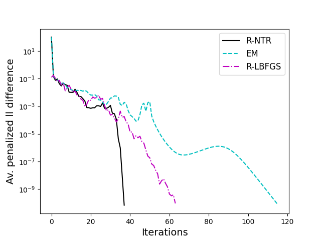
(a) Average penalized log-likelihood red.

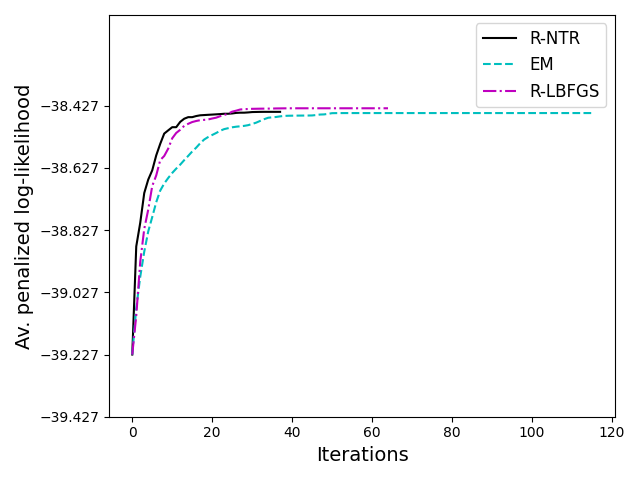
(b) Average penalized log-likelihood

Figure 4.1: Average penalized log-likelihood reduction (a) and average penalized log-likelihood (b) for highly overlapping clusters: $d=20$, $K=5$, $e=1$, $c=0.2$.

Table 4.1: Simulation results of $20$ runs for dimensions $d=20$, number of components $K=5$ and eccentricity $e=1$

		EM	R-NTR	R-LBFGS
c=0.2	Iterations	295	79.4	113.4
	Mean time (s)	3.833	2.716	16.008
	Mean ALL	-42.64	-42.63	-42.63
	MSE weights	0.00139	0.00143	0.008
	MSE means	0.14	0.14	0.13
	MSE cov	2.27	2.5	2.28
c=1	Iterations	262	47.5	102.7
	Mean time (s)	3.65	2.069	14.281
	Mean ALL	-41.2	-41.21	-41.21
	MSE weights	0.00909	0.00985	0.008
	MSE means	0.23	0.22	0.24
	MSE cov	0.67	0.56	0.7
c=5	Iterations	208.8	54.2	92.4
	Mean time (s)	2.747	2.123	12.975
	Mean ALL	-36.98	-36.98	-36.99
	MSE weights	0.00264	0.00282	0.008
	MSE means	0.15	0.17	0.16
	MSE cov	9.81	7.1	10.19

Table 4.2: Simulation results of $20$ runs for dimensions $d=20$, number of components $K=5$ and eccentricity $e=10$

		EM	R-NTR	R-LBFGS
c=0.2	Iterations	66.2	16	33.2
	Mean time (s)	0.873	0.798	4.012
	Mean ALL	-60.06	-60.06	-60.07
	MSE weights	3e-05	3e-05	0.008
	MSE means	0.07	0.07	0.07
	MSE cov	0.31	0.23	0.31
c=1	Iterations	56.6	17.4	30
	Mean time (s)	0.748	0.818	3.624
	Mean ALL	-62.82	-62.82	-62.83
	MSE weights	3e-05	3e-05	0.008
	MSE means	0.09	0.09	0.09
	MSE cov	0.17	0.16	0.17
c=5	Iterations	43.1	14.7	29
	Mean time (s)	0.617	0.748	3.378
	Mean ALL	-61.04	-61.04	-61.05
	MSE weights	4e-05	4e-05	0.008
	MSE means	0.08	0.08	0.08
	MSE cov	0.13	0.14	0.13

In Table (4.3), we show results for dimension $d=40$ and low eccentricity ($e=1$) and the same simulation protocol as above (in particular, $m=1000$). We observed that with our method, we only performed very few Newton-like steps and instead exceeded the trust-region within the tCG many times, leading to poorer steps (see also Figure 2(b)). One possible reason is that the number of parameters increases with $d$ quadratically, that is in $\mathcal{O}(Kd^{2})$, while at the same time we did not increase the number of observations $m=1000$. If we are too far from a local optimum and the clusters are not well initialized due to few observations, the factor $f_{l}^{i}$ in the Hessian (Theorem 4) becomes small, leading to large potential conjugate gradients steps (see Algorithm 2). Although this affects the E-step in the Expectation Maximization algorithm as well, the effect seems to be much severe in our method.
To underline this, we show simulation results for a higher number of observations, that is, $m=10.000$, in Table 4.4 with the same true parameters $\alpha_{j},\mu_{j},\Sigma_{j}$ as in Table 4.3. As expected, the superiority in runtime of our method becomes visible: The R-NTR method beats Expectation maximization with a factor of $4$. Just like for the case of a lower dimension $d=20$, the mean average log-likelihood and the errors are comparable between our method and EM, whereas R-LBFGS shows slightly worse results although it now attains comparable runtimes to our method.

We thus see that the ratio between number of observations and number of parameters must be large enough in order to benefit from the Hessian information in our method.

Table 4.3: Simulation results of $20$ runs for dimensions $d=40$, number of components $K=5$ and eccentricity $e=1$ with $m=1000$ observations

		EM	R-NTR	R-LBFGS
c=0.2	Iterations	57.4	27.9	40.7
	Mean time (s)	1.332	2.296	6.744
	Mean ALL	-84.7935	-84.79	-84.7895
	MSE weights	0.00023	0.00023	0.008
	MSE means	0.104	0.09	0.104
	MSE cov	0.282	0.196	0.281
c=1	Iterations	61	29	48.6
	Mean time (s)	1.391	2.476	8.282
	Mean ALL	-82.3395	-82.3384	-82.3358
	MSE weights	0.0002	0.0002	0.008
	MSE means	0.076	0.084	0.076
	MSE cov	0.139	0.128	0.14
c=5	Iterations	81.8	28.8	49.2
	Mean time (s)	1.812	2.203	8.62
	Mean ALL	-92.4886	-92.4874	-92.4925
	MSE weights	0.00013	0.00013	0.008
	MSE means	0.08	0.095	0.08
	MSE cov	0.116	0.133	0.117

Table 4.4: Simulation results of $20$ runs for dimensions $d=40$, number of components $K=5$ and eccentricity $e=1$ with $m=10000$ observations

		EM	R-NTR	R-LBFGS
c=0.2	Iterations	350.4	33.2	69.4
	Mean time (s)	53.621	12.455	15.449
	Mean ALL	-86.5717	-86.5718	-86.5731
	MSE weights	0.00043	0.00043	0.008
	MSE means	0.093	0.086	0.093
	MSE cov	0.207	0.195	0.206
c=1	Iterations	495.6	63.6	107.3
	Mean time (s)	79.955	20.739	23.153
	Mean ALL	-84.3783	-84.3779	-84.3797
	MSE weights	0.00062	0.00065	0.008
	MSE means	0.075	0.064	0.076
	MSE cov	0.075	0.038	0.075
c=5	Iterations	260.4	28.8	54
	Mean time (s)	42.6	10.434	11.692
	Mean ALL	-94.5592	-94.5591	-94.5603
	MSE weights	0.00012	0.00013	0.008
	MSE means	0.071	0.086	0.071
	MSE cov	0.045	0.053	0.045

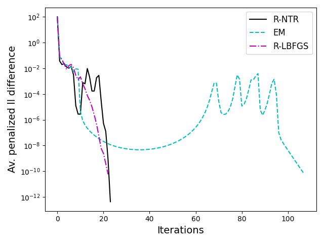
(a) Average penalized log-likelihood red.

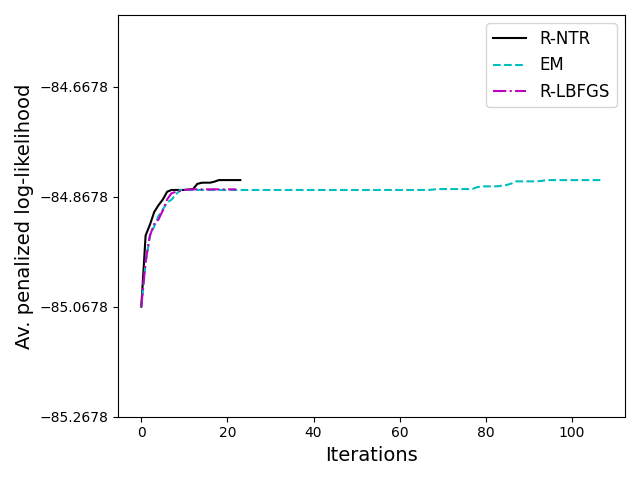
(b) Average penalized log-likelihood

Figure 4.2: Average penalized log-likelihood reduction (a) and average penalized log-likelihood (b) for overlapping clusters: $d=40$, $K=5$, $e=1$, $c=1$.

4.1.2 Real-World Data

We tested our method on some real-world data sets from UCI Machine Learning repository (Dua and Graff, 2017) besides the simulated data sets. For this, we normalized the data sets and tested the methods for different values of $K$.

Combined Cycle Power Plant Data Set (Kaya and Tufekci, 2012).

In Table 4.5, we show the results for the combined cycle power plant data set, which is a data set with $4$ features. Although the dimension is quite low, we see that we can beat EM both in terms of runtime and number of iterations for almost all $K$ by applying the Riemannian Newton-Trust Region method. This underlines the results shown for artificial data in Subsection 4.1.1. The gain by our method becomes even stronger when we consider a large number of components $K$ where the overlap between clusters is large and we can reach a local optimum with our method in up to $15$ times less iterations and a time saving of factor close to $4$.

Table 4.5: Results of (normalized) combined cycle power plant data set for different number of components.Number of observations $m=9568$, dimensions $d=4$.

		EM	R-NTR	R-LBFGS
K = 2	Time (s)	0.40	0.63	2.38
	Iterations	56	19	34
	ALL	-4.24	-4.24	-4.24
K = 5	Time (s)	3.29	2.26	7.50
	Iterations	239	48	70
	ALL	-4.01	-4.01	-4.01
K = 10	Time (s)	31.72	4.28	23.40
	Iterations	1097	58	110
	ALL	-3.83	-3.82	-3.83
K = 15	Time (s)	28.27	6.79	35.77
	Iterations	677	67	111
	ALL	-3.75	-3.75	-3.75

MAGIC Gamma Telescope Data Set (Bock et al., 2004).

We also study the behaviour on a data set with higher dimensions and a larger number of observations with the MAGIC Gamma Telescope Data Set, see Table 4.6. Here, we can also observe a lower number of iterations in the Riemannian Optimization methods. Similar to the combined cycle power plant data set, this effect becomes even stronger for a high number of clusters where the ratio of hidden information is large. Our method shows by far the best runtimes. For this data set, the average log-likelihood values are very close to each other except for $K=15$ where the ALL is worse for the Riemannian methods. It seems that in this case, the R-NTR and the R-LBFGS methods end in different local maxima than the EM. However, for all of the methods, convergence to global maxima is theoretically not ensured and for all methods, a globalization strategy like a split-and-merge approach (Li and Li, 2009) might improve the final ALL values. As the Magic Gamma telescope data set is a classification data set with $2$ classes, we further report the classification performance in Table 7(a). We see that the geodesic distance defined on the manifold and the weighted mean squared errors (wMSE) are comparable between all three methods. In Table 7(b), we also report the Adjusted Rand Index (Hubert and Arabie, 1985) for all methods. Although the clustering performance is very low compared to the true class labels (first row), we see that it is equal among the three methods.

Table 4.6: Results of (normalized) Magic Gamma telescope data set for different number of components. Number of observations $m=19020$, dimensions $d=11$.

		EM	R-NTR	R-LBFGS
K = 2	Time (s)	1.18	0.57	1.52
	Iterations	30	6	17
	ALL	-7.81	-7.81	-7.81
K = 5	Time (s)	3.96	1.32	5.37
	Iterations	65	9	34
	ALL	-6.53	-6.53	-6.53
K = 10	Time (s)	36.00	6.99	20.78
	Iterations	293	34	77
	ALL	-6.02	-6.02	-6.02
K = 15	Time (s)	56.24	12.61	50.52
	Iterations	354	38	115
	ALL	-5.39	-5.54	-5.51

Table 4.7: Model quality for (normalized) magic gamma telescope data set for $K=2$.

(a) geodesic distance and weighted MSE

	EM	R-NTR	R-LBFGS
distance	4.783910	4.783934	4.783922
wMSE weight	0.000034	0.000034	0.000034
wMSE mean	1.883762	1.883765	1.883759
wMSE cov	8.214824	8.214840	8.214828

(b) adjusted rand index

	truth	EM	R-NTR	R-LBFGS
truth	1	0.06	0.06	0.06
EM		1	1.00	1.00
R-NTR			1	1.00
R-LBFGS				1

We show results on additional real-world data sets in Appendix C.

4.2 Gaussian Mixture Models as Density Approximaters

Besides the task of clustering (multivariate) data, Gaussian Mixture Models are also well-known to serve as probability density approximators of smooth density functions with enough components (Scott, 1992).
In this Subsection, we present the applicability of our method for Gaussian mixture density approximation of a Beta-Gamma distribution and compare against EM and R-LBFGS for the estimation of the Gaussian components.

We consider a bivariate Beta-Gamma distribution with parameters $\alpha_{Beta}=0.5$, $\beta_{Beta}=0.5$, $a_{Gamma}=1,\beta_{Gamma}=1$, where the joint distribution is characterized by a Gaussian copula. The density function surface is visualized in Figure 4.3.

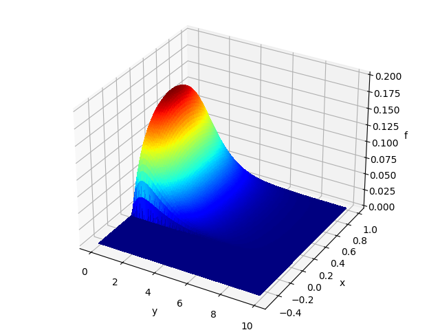
Figure 4.3: Probability density of bivariate Beta($0.5$,$0.5$)-Gamma($1$, $1$) distribution.

We simulated $1000$ realizations of the Beta($0.5$,$0.5$)-Gamma($1$, $1$) distribution and fitted a Gaussian Mixture Model for $100$ simulation runs. We considered different numbers of $K$ and compared the (approximated) root mean integrated squared error (RMISE).
The RMISE and its computational approximation formula is given by (Gross et al., 2015):

$$RMISE(\hat{f}) =\sqrt{\mathbb{E}\left(\int\left(f(x)-\hat{f}(x)\right)^{2}dx\right)}$$

$$\approx\sqrt{\frac{1}{N}\sum\limits_{r=1}^{N}\left(f(g_{r})-\hat{f}(g_{r})\right)^{2}\delta_{g}^{2}},$$

where $f$ denotes the underlying true density , i.e.
Beta($0.5$,$0.5$)-Gamma($1$, $1$), $\hat{f}$ the density approximator (GMM), $N$ is the number of equidistant grid points with the associated grid width $\delta_{g}$.
For our simulation study, we chose $16384$ grid points in the box $[0,5]\times[0,10]$. We show the results in Table 4.8, where we fit the parameters of the GMM by our method (R-NTR) and compare against GMM approximations where we fit the parameters with EM and R-LBFGS. We observe that the RMISE is of comparable size for all methods and even slightly better for our method for $K=2$, $K=5$ and $K=10$. Just as for the clustering results in Subsection 4.1, we have much lower runtimes for R-NTR and a much lower number of total iterations. This is a remarkable improvement especially for a larger number of components. We also observe that in all methods, the mean average log-likelihood (ALL) of the training data sets with $1000$ observations attains higher values with an increasing number of components $K$. This supports the fact that the approximation power of GMMs for arbitrary density function is expected to become higher if we add additional Gaussian components (Scott, 1992, Goodfellow et al., 2016). On the other hand, the RMISE (which is not based on the training data) increased in our experiments with larger $K$’s. This means that we are in a situation of overfitting. The drawback of overfitting is well-known for EM (Andrews, 2018) and we also observed this for the R-NTR and the R-LBFGS methods. However, the RMISE are comparable and so none of the methods outperforms another substantially in terms of overfitting. This can also be seen from Figure 4.4 showing the distribution of the pointwise errors for $K=2$ and $K=5$. Although the R-LBFGS method shows higher error values on the boundary of the support of the distribution for $K=5$, the errors show similar distributions among the three methods at a comparable level. We propose methodologies such as cross validation (Murphy, 2013) or applying a split-and-merge approach on the optimized parameters (Li and Li, 2009) to address the problem of overfitting.

Table 4.8: Simulation results averaged over $100$ simulation runs for approximation of a Beta($0.5$,$0.5$)-Gamma($1$, $1$) distribution by a Gaussian Mixture Models with different values of $K$. Parameter Estimation by EM, R-NTR and R-LBFGS.

		EM	R-NTR	R-LBFGS
K=2	Mean RMISE	0.00453	0.00453	0.00453
	SE RMISE	0.00017	0.00017	0.00017
	Iterations	113	27.9	25.9
	Mean time (s)	0.2002	0.1532	0.9877
	Mean ALL	-1.53103	-1.52953	-1.53103
K=5	Mean RMISE	0.00565	0.00565	0.00567
	SE RMISE	0.00028	0.00024	0.00025
	Iterations	346.5	47	72.9
	Mean time (s)	1.0893	0.5202	6.7941
	Mean ALL	-1.22852	-1.22108	-1.22912
K=10	Mean RMISE	0.00639	0.00643	0.00643
	SE RMISE	0.00025	0.00027	0.00029
	Iterations	623.1	56.8	112.2
	Mean time (s)	3.4226	1.7108	20.4754
	Mean ALL	-1.06821	-1.02844	-1.06781
K=15	Mean RMISE	0.00667	0.00669	0.0067
	SE RMISE	0.00026	0.00027	0.00026
	Iterations	791.5	62.9	135.2
	Mean time (s)	6.1649	2.5701	37.6
	Mean ALL	-1.02677	-0.95907	-1.02604
K=20	Mean RMISE	0.00681	0.00683	0.00685
	SE RMISE	0.00026	0.00025	0.00026
	Iterations	874.8	66.9	144.6
	Mean time (s)	8.7694	3.3773	55.6337
	Mean ALL	-1.02029	-0.9202	-1.02056

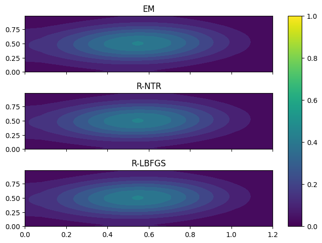
(a) $K=2$

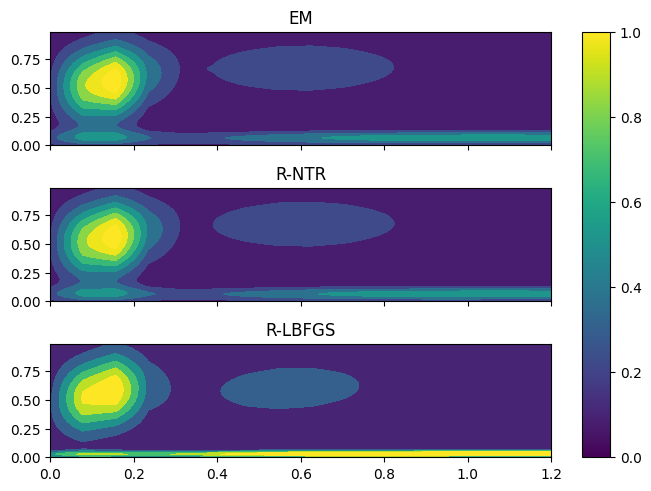
(b) $K=5$

Figure 4.4: Contours of pointwise root mean squared error (RMSE) for density approximation via GMMs of the Beta($0.5$,$0.5$)-Gamma($1$, $1$) distribution.

The results show that our method is well-suited for both density estimation tasks and especially for clustering of real-world and simulated data.

5 Conclusion

We proposed a Riemannian Newton Trust-Region method for Gaussian Mixture Models. For this, we derived an explicit formula for the Riemannian Hessian and gave results on convergence theory. Our method is a fast alternative to the well-known Expectation Maximization and existing Riemannian approaches for Gaussian Mixture Models. Especially for highly overlapping components, the numerical results show that our method leads to an enourmous speed-up both in terms of runtime and the total number of iterations and medium-sized problems. This makes it a favorable method for density approximation as well as for difficult clustering tasks for data with higher dimensions. Here, especially the availability of the Riemannian Hessian increases the convergence speed compared to Quasi-Newton algorithms. When considering higher-dimensional data, we experimentally observed that our method still works very well and is faster than EM if the number of observations is large enough. We plan to examine this further and take a look into data sets with higher dimensions. Here, it is common to impose a special structure on the covariance matrices to tackle the curse of dimensionality (McLachlan et al., 2019). Adapted versions for Expectation Maximization exist and a transfer of Riemannian method into constrained settings is subject of current research.

Appendix A Unboundedness of the Reformulated Problem

Theorem 7

The reformulated objective (3) without penalization term is unbounded from above.

Proof. We show that there exists $\theta_{s}$ such that $\lim\limits_{\theta\rightarrow\theta_{s}}\hat{\mathcal{L}}(\theta)=\infty$.
We consider the simplified case where $K=1$ and investigate the log-likelihood of the variable $\theta^{(n)}=S^{(n)}$ since $\alpha_{1}=1$. Similar to the proof of Theorem 2, we introduce a singular positive semidefinite matrix $S_{s}$ with rank $r<d+1$ and a sequence of positive definite matrices $S_{1}^{(n)}$ converging to $S_{s}$ for $n\rightarrow\infty$. The reformulated objective at $\theta^{(n)}$ reads

$$\hat{\mathcal{L}}\left(\theta^{(n)}\right)=\sum\limits_{i=1}^{m}\left(\log\left(\frac{1}{(2\pi)^{d/2}}\frac{\exp(\frac{1}{2}(1-{y_{i}}^{T}({S_{1}}^{(n)})^{-1}y_{i}))}{\det\left(S_{1}^{(n)}\right)^{1/2}}\right)\right).$$ (38)

With the decomposition $(S_{1}^{(n)})^{-1}=U^{T}D^{n}U$ as in (14), we see that

$$y_{i}^{T}(S_{1}^{(n)})^{-1}y_{i}=\sum\limits_{l=1}^{d-r-1}\frac{\left((Uy_{i})_{l}\right)^{2}}{\lambda_{l}}+\sum\limits_{l=d-r}^{d+1}\frac{\left((Uy_{i})_{l}\right)^{2}}{\lambda_{l}}$$

Now assume that one of the $y_{i}$ is in the kernel of the matrix $\tilde{U}_{s}$, where

$$\tilde{U}_{s}=\left(\begin{array}[]{ccc}u_{11}&\dots&u_{1(d-r-1)}\\ \vdots&\ddots&\vdots\\ u_{(d-r-1)1}&\dots&u_{(d-r-1)(d-r-1)}\end{array}\right).$$

Then we see that (38) reads

$$\hat{\mathcal{L}}\left(\theta^{(n)}\right)=\sum\limits_{i=1}^{m}\bigg{[}\log\bigg{(}\frac{1}{(2\pi)^{d/2}}\frac{1}{\lambda^{(n)}\lambda^{+}}\exp\bigg{(}\frac{1}{2}\bigg{(}1-\sum\limits_{l=r-d}^{d+1}\frac{\left((Uy_{i})_{l}\right)^{2}}{\lambda_{l}}\bigg{)}\bigg{)}\bigg{)}\bigg{]}\underrightarrow{n\rightarrow\infty}\quad\infty,$$

where $\lambda^{(n)}=\prod\limits_{1}^{d-r-1}\lambda_{l}^{(n)}$ and $\lambda^{+}=\prod\limits_{d-r}^{d+1}\lambda_{l}$ as in the proof of Theorem 2.

Appendix B Truncated Conjugate Gradient Method

We here state the truncated CG method to solve the quadratic subproblem in the Riemannian Newton Trust-Region Algorithm, line 3 in Algorithm 1.

Input: Riemannian gradient $\operatorname{grad}f(\theta^{t})$, linear operator $H_{t}$, inner product $\langle\cdot,\cdot\rangle_{\theta^{t}}$, optional preconditioner $M_{t}$, TR radius $\Delta_{t}$, termination parameter $\delta$, $\kappa$

1 Set $s_{0}=0$, $r_{0}=\operatorname{grad}f(\theta^{t})$, $z_{0}=M_{t}r_{0}$, $p_{0}=-z_{0}$;

2 for $n=0,1,2,\dots$ do

3       if $\langle p_{n},H_{t}[p_{n}]\rangle_{\theta^{t}}\leq 0$ then

4             Compute $\tau^{tCG}=\arg\min\limits_{\tau}\hat{m}_{\theta^{t}}(s_{n}+\tau p_{n})$ s.t. $\left\lVert s_{n}+\tau p_{n}\right\rVert_{\theta^{t}}=\Delta_{t}$;

5             Set $s_{n+1}=s_{n}+\tau^{tCG}p_{n}$;

6             return $s_{n+1}$;

7       Compute ${\alpha_{n}^{tCG}}=\frac{\langle r_{n},z_{n}\rangle_{\theta^{t}}}{\langle p_{n},H_{t}[p_{n}]\rangle_{\theta_{t}}}$;

8       if $\left\lVert s_{n}+\alpha_{n}^{tCG}p_{n}\right\rVert_{\theta^{t}}>\Delta_{t}$ then

9             Compute $\tau^{tCG}=\arg\min\limits_{\tau}\hat{m}_{\theta^{t}}(s_{n}+\tau p_{n})$ s.t. $\left\lVert s_{n}+\tau p_{n}\right\rVert_{\theta^{t}}=\Delta_{t}$;

10             Set $s_{n+1}=s_{n}+\tau^{tCG}p_{n}$;

11             return $s_{n+1}$;

12      else

13             $s_{n+1}=s_{n}+\alpha_{n}^{tCG}p_{n}$;

14             $r_{n+1}=r_{n}+\alpha_{n}^{tCG}H_{t}[p_{n}]$;

15             $z_{n+1}=M_{t}r_{n+1}$;

16             $\beta_{n+1}^{tCG}=\frac{\langle z_{n+1}z_{n+1}\rangle_{\theta^{t}}}{\langle z_{n},z_{n}\rangle_{\theta^{t}}}$;

17             $p_{n+1}=-z_{n+1}+\beta_{n+1}^{tCG}p_{n}$;

18             if $\left\lVert r_{n+1}\right\rVert_{\theta^{t}}\leq\left\lVert r_{0}\right\rVert_{\theta^{t}}\min(\left\lVert r_{0}\right\rVert_{\theta^{t}}^{\delta},\kappa)$ then

19                   return $s_{n+1}$;

20            

21      

22 end for

23

Algorithm 2 Truncated Conjugate Gradient Method Absil et al. (2008)

Appendix C Additional Numerical Results

We present numerical results additional to Section 4 both for simulated clustering data and for real-world data.

C.1 Simulated data

Table C.1: Simulation results of $20$ runs for dimensions $d=20$, number of components $K=5$ and eccentricity $e=5$ with $n=1000$ observations.

		EM	R-NTR	R-LBFGS
c=0.2	Iterations	145.7	38.5	60.4
	Mean time (s)	1.899	1.512	8.165
	Mean ALL	-50.65	-50.66	-50.66
	MSE weights	0.00018	0.00019	0.008
	MSE means	0.08	0.08	0.08
	MSE cov	2.18	1.83	2.21
c=1	Iterations	258.9	60.4	84.1
	Mean time (s)	3.061	1.951	11.64
	Mean ALL	-57.65	-57.65	-57.65
	MSE weights	0.00037	0.0004	0.008
	MSE means	0.08	0.07	0.07
	MSE cov	1.02	1.39	1.04
c=5	Iterations	194.6	37.2	65.7
	Mean time (s)	2.367	1.267	8.927
	Mean ALL	-54.86	-54.86	-54.87
	MSE weights	0.00017	0.00018	0.008
	MSE means	0.07	0.07	0.07
	MSE cov	0.15	0.13	0.15

Table C.2: Simulation results of $20$ runs for dimensions $d=40$, number of components $K=5$ and eccentricity $e=10$ for different number of observations

(a) $n=1000$ observations

		EM	R-NTR	R-LBFGS
c=0.2	Iterations	4	16.3	6.6
	Mean time (s)	0.091	1.336	0.622
	Mean ALL	-125.63	-125.63	-125.649
	MSE weights	3e-05	3e-05	0.008
	MSE means	0.091	0.095	0.091
	MSE cov	0.224	0.215	0.224
c=1	Iterations	4	17.6	8.8
	Mean time (s)	0.097	1.561	0.862
	Mean ALL	-110.112	-110.112	-110.14
	MSE weights	3e-05	3e-05	0.008
	MSE means	0.089	0.084	0.089
	MSE cov	0.461	0.337	0.461
c=5	Iterations	4	17	7.2
	Mean time (s)	0.094	1.497	0.697
	Mean ALL	-116.276	-116.276	-116.3
	MSE weights	3e-05	3e-05	0.008
	MSE means	0.061	0.066	0.061
	MSE cov	0.351	0.43	0.351

(b) $n=10.000$ observations

		EM	R-NTR	R-LBFGS
c=0.2	Iterations	4	2.3	3.3
	Mean time (s)	0.628	1.524	0.74
	Mean ALL	-127.762	-127.762	-127.764
	MSE weights	0	0	0.008
	MSE means	0.089	0.09	0.089
	MSE cov	0.14	0.189	0.14
c=1	Iterations	4	2.8	3.8
	Mean time (s)	0.609	1.676	0.884
	Mean ALL	-112.25	-112.25	-112.252
	MSE weights	0	0	0.008
	MSE means	0.084	0.084	0.084
	MSE cov	0.313	0.29	0.313
c=5	Iterations	4	2.6	3.6
	Mean time (s)	0.63	1.662	0.774
	Mean ALL	-118.337	-118.337	-118.339
	MSE weights	0	0	0.008
	MSE means	0.065	0.071	0.065
	MSE cov	0.228	0.235	0.228

C.2 Real-world datasets

C.2.1 Gas Turbine CO and NOx Emission Data Set (Kaya et al., 2019)

Table C.3: Results of (normalized) Magic Gamma telescope data set for different number of components $K$. Number of observations $m=36733$, dimensions $d=11$.

		EM	R-NTR	R-LBFGS
K = 2	Time (s)	2.04	2.48	3.22
	Iterations	25	22	28
	ALL	-5.73	-5.73	-5.73
K = 5	Time (s)	17.41	9.52	11.48
	Iterations	90	46	58
	ALL	-1.93	-1.99	-1.93
K = 10	Time (s)	40.66	29.36	27.31
	Iterations	130	61	75
	ALL	-1.17	-1.16	-1.17
K = 15	Time (s)	52.06	63.20	142.77
	Iterations	115	76	233
	ALL	0.04	-0.04	-0.05

C.2.2 Wine Quality Data set (Cortez et al., 2009)

Table C.4: Results of (normalized) Wine quality data set for different number of components $K$. Number of observations $m=6497$ , dimensions $d=11$.

		EM	R-NTR	R-LBFGS
K = 2	Time (s)	0.54	0.24	1.55
	Iterations	27	8	20
	ALL	-11.02	-11.02	-11.02
K = 5	Time (s)	4.75	1.24	5.69
	Iterations	154	34	51
	ALL	-9.74	-9.98	-9.88
K = 10	Time (s)	12.61	5.65	22.80
	Iterations	239	83	100
	ALL	-9.23	-9.28	-9.28
K = 15	Time (s)	91.16	11.17	51.65
	Iterations	1137	70	147
	ALL	-8.91	-8.88	-8.89

The wine quality data set also provides classification labels: we can distinguish between white and red wine or distinguish between 7 quality labels. Besides the clustering performance of the methods (Table C.4), we also show the goodness of fit of our method for $K=2$ and $K=7$.

Table C.5: Model quality for (normalized) wine data set for $K=2$ (red/white wine).

(a) Weighted mean squared errors of
(normalized) wine data set for $K=2$.
Weighting by mixing coefficients
of the respective method.

	EM	R-NTR	R-LBFGS
distance	2.757966	2.757982	2.757974
wMSE weight	0.003169	0.003169	0.003169
wMSE mean	0.073776	0.073779	0.073778
wMSE cov	0.562106	0.562113	0.562109

(b) Adjusted Rand Index for (normalized) wine data set for $K=2$.

	truth	EM	R-NTR	R-LBFGS
truth	1	0.02	0.01	0.02
EM		1	0.73	0.70
R-NTR			1	0.85
R-LBFGS				1

Table C.6: Model quality for (normalized) wine data set for $K=7$ (quality label).

(a) Weighted mean squared errors of
(normalized) wine data set for $K=7$.
Weighting by mixing coefficients
of the respective method.

	EM	R-NTR	R-LBFGS
distance	89.259333	89.488919	88.894978
wMSE weight	0.019019	0.010065	0.035496
wMSE mean	6.068149	5.617490	11.996024
wMSE cov	61.808676	37.060684	55.707085

(b) Adjusted Rand Index for (normalized) wine data set for $K=7$.

	truth	EM	R-NTR	R-LBFGS
truth	1	0.02	0.01	0.02
EM		1	0.73	0.70
R-NTR			1	0.85
R-LBFGS				1

References

- Absil et al. (2008) P.-A. Absil, R. Mahony, and R. Sepulchre. Optimization Algorithms on Matrix Manifolds. Princeton University Press, Princeton, NJ, 2008. ISBN 978-0-691-13298-3.
- Alfò et al. (2008) M. Alfò, L. Nieddu, and D. Vicari. A finite mixture model for image segmentation. Statistics and Computing, 18(2):137–150, June 2008. ISSN 0960-3174. doi: 10.1007/s11222-007-9044-9. URL https://doi.org/10.1007/s11222-007-9044-9.
- Andrews (2018) J. L. Andrews. Addressing overfitting and underfitting in gaussian model-based clustering. Computational Statistics and Data Analysis, 127:160–171, 2018. ISSN 0167-9473. URL https://doi.org/10.1016/j.csda.2018.05.015.
- Arthur and Vassilvitskii (2007) D. Arthur and S. Vassilvitskii. k-means++: The advantages of careful seeding. In SODA ’07: Proceedings of the eighteenth annual ACM-SIAM symposium on Discrete algorithms, pages 1027–1035, Philadelphia, PA, USA, 2007. Society for Industrial and Applied Mathematics. ISBN 978-0-898716-24-5.
- Articus and Burgard (2014) C. Articus and J. P. Burgard. A Finite Mixture Fay Herriot-type model for estimating regional rental prices in Germany. Research Papers in Economics 2014-14, University of Trier, Department of Economics, 2014. URL https://ideas.repec.org/p/trr/wpaper/201414.html.
- Bhatia (2007) R. Bhatia. Positive Definite Matrices. Princeton Series in Applied Mathematics. Princeton University Press, Princeton, NJ, USA, 2007.
- Bishop (2006) C. M. Bishop. Pattern Recognition and Machine Learning (Information Science and Statistics). Springer-Verlag, Berlin, Heidelberg, 2006. ISBN 0387310738.
- Bock et al. (2004) R. Bock, A. Chilingarian, M. Gaug, F. Hakl, T. Hengstebeck, M. Jiřina, J. Klaschka, E. Kotrč, P. Savický, S. Towers, A. Vaiciulis, and W. Wittek. Methods for multidimensional event classification: a case study using images from a cherenkov gamma-ray telescope. Nuclear Instruments and Methods in Physics Research Section A: Accelerators, Spectrometers, Detectors and Associated Equipment, 516(2):511–528, 2004. ISSN 0168-9002. URL https://doi.org/10.1016/j.nima.2003.08.157.
- Boumal (2020) N. Boumal. An introduction to optimization on smooth manifolds. Available online, Nov 2020. URL http://www.nicolasboumal.net/book.
- Carmo (1992) M. P. . d. Carmo. Riemannian geometry. Mathematics theory and applications. Birkhäuser, Boston, 1992. ISBN 0-8176-3490-8.
- Compiani and Kitamura (2016) G. Compiani and Y. Kitamura. Using Mixtures in Econometric Models: A Brief Review and Some New Results. The Econometrics Journal, 19(3):C95–C127, 10 2016. ISSN 1368-4221. doi: 10.1111/ectj.12068. URL https://doi.org/10.1111/ectj.12068.
- Conn et al. (2000) A. R. Conn, N. I. Gould, and P. L. Toint. Trust-region methods. MPS-SIAM series on optimization. SIAM Society for Industrial and Applied Mathematics, Philadelphia, 2000. ISBN 0898714605.
- Coretto (2021) P. Coretto. Estimation and computations for gaussian mixtures with uniform noise under separation constraints. Statistical Methods and Applications, 07 2021. doi: 10.1007/s10260-021-00578-2.
- Cortez et al. (2009) P. Cortez, A. Cerdeira, F. Almeida, T. Matos, and J. Reis. Modeling wine preferences by data mining from physicochemical properties. Decision Support Systems, 47(4):547–553, 2009. ISSN 0167-9236. URL https://doi.org/10.1016/j.dss.2009.05.016. Smart Business Networks: Concepts and Empirical Evidence.
- Dasgupta (1999) S. Dasgupta. Learning mixtures of gaussians. In Proceedings of the 40th Annual Symposium on Foundations of Computer Science, FOCS ’99, page 634, USA, 1999. IEEE Computer Society. ISBN 0769504094.
- Dresvyanskiy et al. (2020) D. Dresvyanskiy, T. Karaseva, V. Makogin, S. Mitrofanov, C. Redenbach, and E. Spodarev. Detecting anomalies in fibre systems using 3-dimensional image data. Stat. Comput., 30(4):817–837, 2020. doi: 10.1007/s11222-020-09921-1. URL https://doi.org/10.1007/s11222-020-09921-1.
- Dua and Graff (2017) D. Dua and C. Graff. UCI machine learning repository, 2017. URL http://archive.ics.uci.edu/ml.
- Goodfellow et al. (2016) I. Goodfellow, Y. Bengio, and A. Courville. Deep Learning. MIT Press, 2016. http://www.deeplearningbook.org.
- Gould et al. (2005) N. Gould, D. Orban, A. Sartenaer, and P. Toint. Sensitivity of trust-region algorithms to their parameters. 4OR quarterly journal of the Belgian, French and Italian Operations Research Societies, 3:227–241, 2005. doi: 10.1007/s10288-005-0065-y.
- Gross et al. (2015) M. Gross, U. Rendtel, T. Schmid, S. Schmon, and N. Tzavidis. Estimating the density of ethnic minorities and aged people in Berlin. 2015.
- Heidel and Schulz (2018) G. Heidel and V. Schulz. A riemannian trust-region method for low-rank tensor completion. Numer. Linear Algebra Appl., 25(6), 2018.
- Hosseini and Mash’al (2015) R. Hosseini and M. Mash’al. Mixest: An estimation toolbox for mixture models. CoRR, abs/1507.06065, 2015. URL http://arxiv.org/abs/1507.06065.
- Hosseini and Sra (2015) R. Hosseini and S. Sra. Matrix manifold optimization for gaussian mixtures. In Advances in Neural Information Processing Systems, volume 28. Curran Associates, Inc., 2015.
- Hosseini and Sra (2020) R. Hosseini and S. Sra. An alternative to EM for gaussian mixture models: batch and stochastic riemannian optimization. Math. Program., 181(1):187–223, 2020.
- Hubert and Arabie (1985) L. Hubert and P. Arabie. Comparing partitions. Journal of classification, 2(1):193–218, 1985.
- Jeuris et al. (2012) B. Jeuris, R. Vandebril, and B. Vandereycken. A survey and comparison of contemporary algorithms for computing the matrix geometric mean. ETNA, 39:379–402, 2012.
- Kaya and Tufekci (2012) H. Kaya and P. Tufekci. Local and global learning methods for predicting power of a combined gas and steam turbine. 2012.
- Kaya et al. (2019) H. Kaya, P. Tüfekci, and E. Uzun. Predicting co and nox emissions from gas turbines: novel data and a benchmark pems. Turkish Journal of Electrical Engineering and Computer Science, 27:4783 – 4796, 2019.
- Lee and Mclachlan (2013) S. Lee and G. Mclachlan. On mixtures of skew normal and skew [tex equation: t] -distributions. Advances in Data Analysis and Classification, 7, 09 2013. doi: 10.1007/s11634-013-0132-8.
- Li and Li (2009) Y. Li and L. Li. A novel split and merge em algorithm for gaussian mixture model. In 2009 Fifth International Conference on Natural Computation, volume 6, pages 479–483, 2009. doi: 10.1109/ICNC.2009.625.
- Ma et al. (2000) J. Ma, L. Xu, and M. Jordan. Asymptotic convergence rate of the em algorithm for gaussian mixtures. Neural Comput., 12:2881–2907, 2000.
- McLachlan et al. (2019) G. J. McLachlan, S. X. Lee, and S. I. Rathnayake. Finite mixture models. Annual Review of Statistics and Its Application, 6(1):355–378, 2019. doi: 10.1146/annurev-statistics-031017-100325.
- Morales and Nocedal (2000) J. Morales and J. Nocedal. Automatic preconditioning by limited memory quasi-newton updating. SIAM Journal on Optimization, 10:1079–1096, 06 2000.
- Murphy (2013) K. P. Murphy. Machine learning : a probabilistic perspective. MIT Press, Cambridge, Mass., 2013. ISBN 9780262018029 0262018020.
- Naim and Gildea (2012) I. Naim and D. Gildea. Convergence of the em algorithm for gaussian mixtures with unbalanced mixing coefficients. In Proceedings of the 29th International Coference on International Conference on Machine Learning, ICML’12, page 1427–1431, Madison, WI, USA, 2012. Omnipress. ISBN 9781450312851.
- Ormoneit and Tresp (1995) D. Ormoneit and V. Tresp. Improved gaussian mixture density estimates using bayesian penalty terms and network averaging. In Proceedings of the 8th International Conference on Neural Information Processing Systems, NIPS’95, page 542–548, Cambridge, MA, USA, 1995. MIT Press.
- Salakhutdinov et al. (2003) R. Salakhutdinov, S. Roweis, and Z. Ghahramani. Optimization with em and expectation-conjugate-gradient. In Proceedings of the Twentieth International Conference on International Conference on Machine Learning, ICML’03, page 672–679. AAAI Press, 2003. ISBN 1577351894.
- Sartenaer (1997) A. Sartenaer. Automatic determination of an initial trust region in nonlinear programming. SIAM J. Sci. Comput., 18(6):1788–1803, Nov. 1997. ISSN 1064-8275 (print), 1095-7197 (electronic).
- Scott (1992) D. Scott. Multivariate Density Estimation. Theory, Practice, and Visualization. Wiley Series in Probability and Mathematical Statistics. John Wiley and Sons, New York, London, Sydney, 1992.
- Snoussi and Mohammad-Djafari (2002) H. Snoussi and A. Mohammad-Djafari. Penalized maximum likelihood for multivariate gaussian mixture. AIP Conference Proceedings, 617(1):36–46, 2002.
- Sra and Hosseini (2015) S. Sra and R. Hosseini. Conic geometric optimization on the manifold of positive definite matrices. SIAM J. Optim., 25:713–739, 2015.
- Townsend et al. (2016) J. Townsend, N. Koep, and S. Weichwald. Pymanopt: A python toolbox for optimization on manifolds using automatic differentiation. Journal of Machine Learning Research, 17(137):1–5, 2016. URL http://jmlr.org/papers/v17/16-177.html.
- Vanderbei and Benson (1999) R. J. Vanderbei and H. Y. Benson. On formulating semidefinite programming problems as smooth convex nonlinear optimization problems. Computational Optimization and Applications, 13(1):231–252, 1999.
- Wu et al. (2012) B. Wu, C. A. Mcgrory, and A. N. Pettitt. A new variational bayesian algorithm with application to human mobility pattern modeling. Statistics and Computing, 22(1):185–203, Jan. 2012. ISSN 0960-3174. doi: 10.1007/s11222-010-9217-9. URL https://doi.org/10.1007/s11222-010-9217-9.
- Xu and Jordan (1996) L. Xu and M. I. Jordan. On convergence properties of the em algorithm for gaussian mixtures. Neural Comput., 8(1):129–151, 1996. ISSN 0899-7667.
- Zoran and Weiss (2012) D. Zoran and Y. Weiss. Natural images, gaussian mixtures and dead leaves. Advances in Neural Information Processing Systems, 3:1736–1744, 01 2012.