Analysis of Molecular Communications on the Growth Structure of Glioblastoma Multiforme

Abstract

In this paper we consider the influence of intercellular communication on the development and progression of Glioblastoma Multiforme (GBM), a grade IV malignant glioma which is defined by an interplay Grow i.e. self renewal and Go i.e. invasiveness potential of multiple malignant glioma stem cells. Firstly, we performed wet lab experiments with U87 malignant glioma cells to study the node-stem growth pattern of GBM. Next we develop a model accounting for the structural influence of multiple transmitter and receiver glioma stem cells resulting in the node-stem growth structure of GBM tumour. By using information theory we study different properties associated with this communication model to show that the growth of GBM in a particular direction (node to stem) is related to an increase in mutual information. We further show that information flow between glioblastoma cells for different levels of invasiveness vary at different points between node and stem. These findings are expected to contribute significantly in the design of future therapeutic mechanisms for GBM.

I Introduction

The inter-disciplinary research field of molecular communications bridges across different discipline such as biological sciences and communication engineering formulating an internet of nano-bio things [1]. Molecular communication relies on information carrying signalling molecules as well as intercellular communications to encode the information to be transmitted. These molecules propagate through a medium by using diffusion [2] or active transport [3]. The incoming molecules are captured at the receiver end, enabling the decoding of input signal [4]. The past decade has experienced a growing interest in applications of molecular communication in biomedical research. One such application is to study dynamic processes underlying the progression or growth of Glioblastoma Multiforme (GBM). GBM tumourigenesis relies on the dynamics of molecular communication networks in an interplay between ‘transmitter’ and ‘receiver’ glioma stem cells (GSCs) giving rise to GBM tumour invasion and progression. In this process the key role is performed by inter cellular communications between GSCs and Glioma Cells (GCs) [5].

In recent literature researchers have proposed a novel molecular communication based therapeutic mechanism to tackle GBM [6]. In our previous work [7] we proposed a simple voxel model to study the role of inter-cellular communication in the growth of GBM. However, the influence of cell-cell interactions (communications) on the structural formation of GBM during their self-organisation process still remains an outstanding issue. In order to develop an optimal therapeutic mechanism for GBM we aim to address this gap in knowledge. In particular this paper aims to study the role of intercellular communication in the evolution of GBM structure as a molecular communication network. The specific contributions of this paper are: (a) Mathematical model for inter-cellular molecular communication for multiple transmitter and receiver GSCs (self-proliferating) and Glioma (invasive) cells resulting in GBM tumour growth. (b) To account for the self organization role of Glioblastoma cells to form a structure comprising of node and stem in a particular direction depending on the mutual information between malignant glioma cells which evolve to the highest grade tumour, i,e. GBM. By studying the impact of mutual information at various locations (i.e. between node and stem cell or within stem cells) we can utilise this knowledge to design future therapeutic mechanisms for GBM.

The rest of the paper is organized as follows. In Section II we present the system model which includes the transmission and propagation mechanisms. Section III presents the complete molecular communication system model including diffusion and reactions. Next in Section IV we derive expressions for mutual information for multiple cells and follow it up with expressions of information propagation speed and GBM growth. Next in Sections V and VI we present numerical results and conclusion respectively.

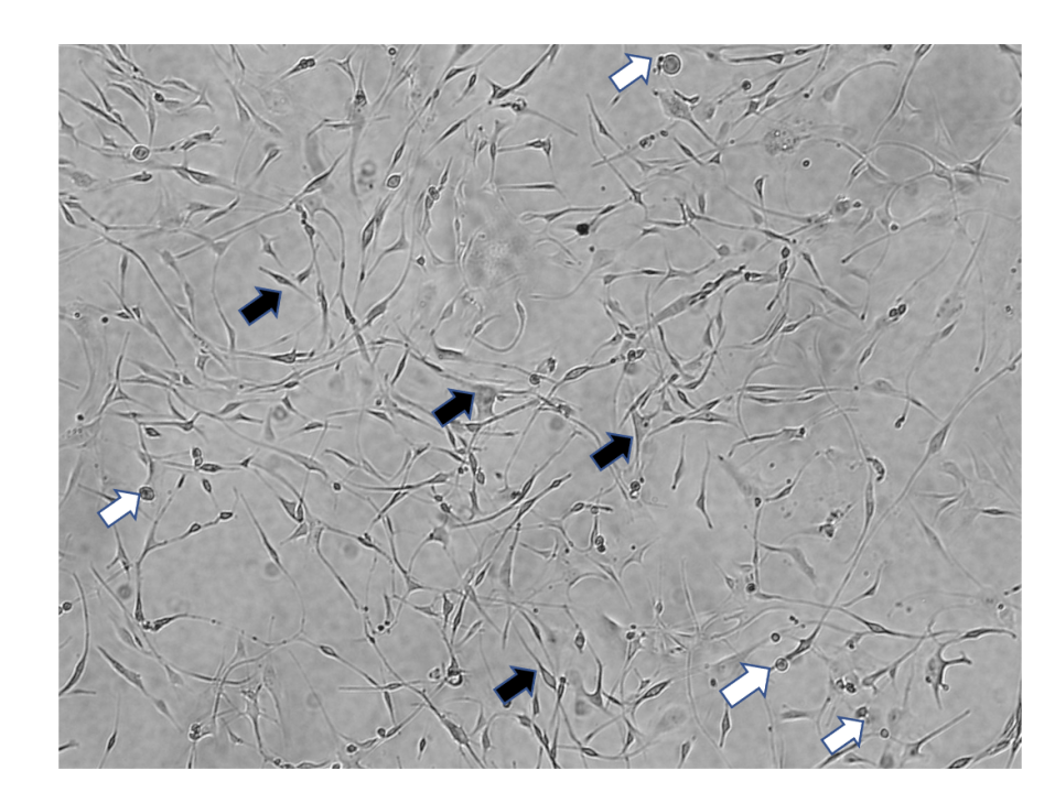
Figure 1: Grade IV U87 Malignant Glioma Cells in culture- White arrows represent Grow (GSC) and black arrows represent Grow (malignant GC).

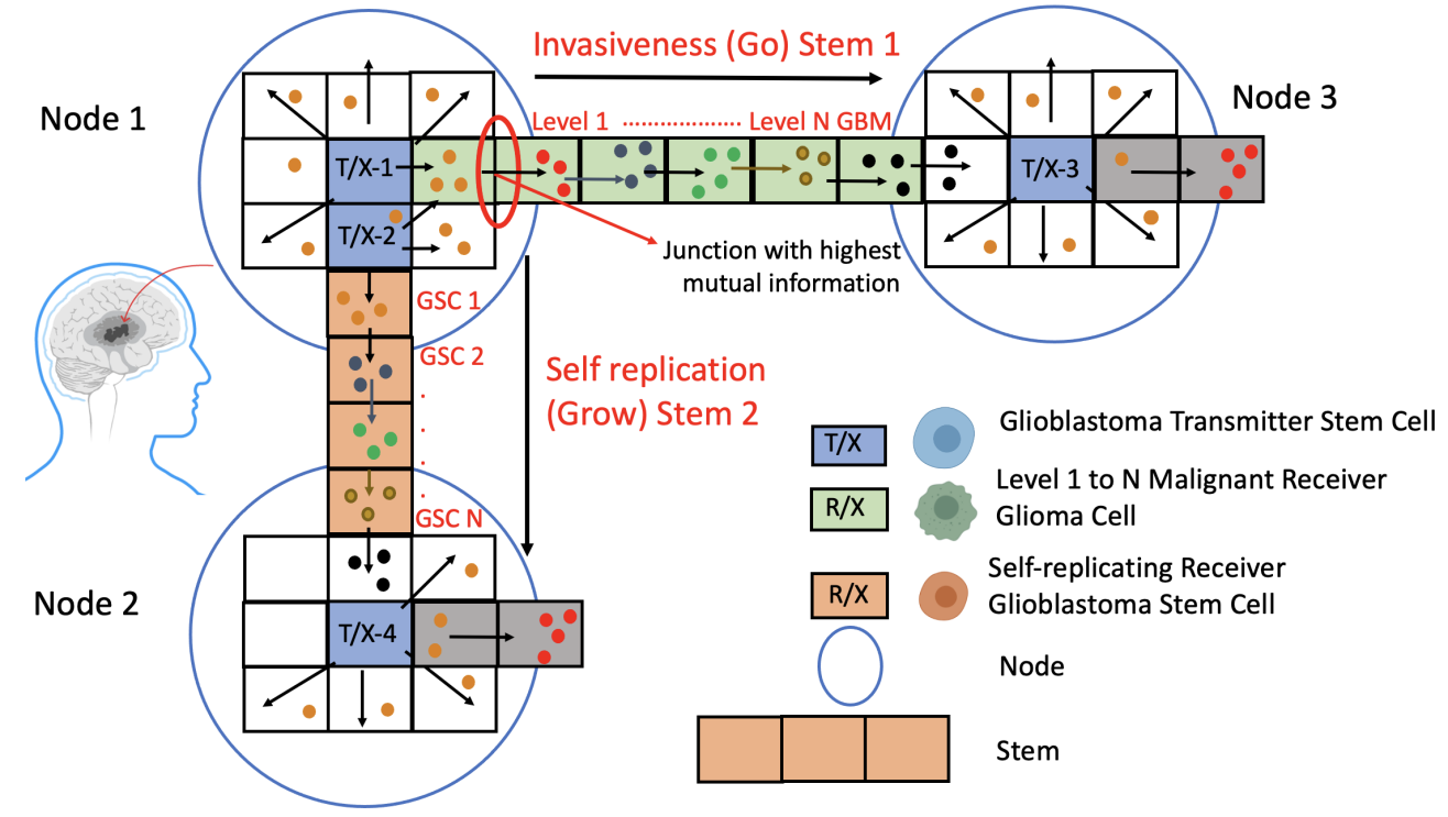
Figure 2: Evolution of Go and Grow based node-stem structure of GSC cells leading to GBM growth.

II System Model

In this section we present the system model accounting for the influence of multiple transmitter and receiver glioma cells on the structure of GBM. From literature we learn that errors in internal signalling of neurons result in the generation of a glioma stem cell (GSC) [8]. This GSC acts as an initiator to generate and progress GBM tumour by using inter-cellular molecular communication. Figure 1 shows the wet lab experimental results for the growth pattern of U87 malignant glioma cells. The white arrows in Figure 1 show spheroid cells representing Glioma Stem Cells whereas black arrows show malignant glioma cells (GBM) at different levels of invasiveness. For both these cases we observe a node-stem structure associated with growth of GBM. In this paper we present a theoretical model to explain these experimental results where a higher mutual information between multiple cells result in this node-stem growth structure of GBM. Figure 2 shows GBM growth as a cell signalling network comprising of multiple transmitter and receiver malignant glioma cells which leads to GBM tumour growth through: (a) self-renewing GSCs i.e. Grow and (b) invasiveness from level $1$ to level $N$ GBM i.e. Go (c) Hybrid of Grow and Go. Figure 1 shows the self-organization of malignant cells to form a node-stem structure (using inter-cellular communication). The transmitter glioma stem cells T/X-1 and T/X-2 (i.e. node) emit signalling molecules that diffuse through propagation medium to the neighbouring cells in different directions. However, the self-replication (i.e. Grow configuration) up to $N$ GSC receiver cells in one direction (i.e. stem growth) depends on the mutual information at each junction (i.e. boundary with neighbouring cell/voxel) leading to the increased growth of GBM in the direction of higher information flow. Similarly we can consider the invasiveness of GSC cells (i.e. Go configuration) from level $1$ to level $N$ GBM increasing more in one particular direction depending on the mutual information at the junction.

Figure 1 shows the node-stem structure for both Grow and Go configurations for multiple transmitter cells. The input information molecules at each step (cell) along the length of stem propagate to the receiver malignant glioma cells through diffusion leading to chemical reactions which produce output molecules. In this work we study how varying number of transmitter and receiver cells can influence the node-stem structure of GBM. By using mathematical modelling we show that the GBM growth rate in different directions depend directly on the mutual information between malignant glioma cells. Note that the example presented is for two transmitter cells, however it is straightforward to extend this general model to incorporate increasing number of transmitters cells.

II-A Transmitter and Propagation Mechanism

In order to model the transmission and propagation we use a previously developed voxel based model for intercellular molecular communication [9, 10]. Each transmitter is assumed to occupy a single voxel emitting input molecules $P$ at a rate of $U_{i}(t)$. For multiple transmitter cells the different levels of input signals correspond to different input concentrations of molecules. Considering example in Figure 1, the information carrying molecules emitted by the transmitter diffuse through a propagation medium to the neighbouring receiver cells resulting in tumour growth due to Go diffusion and Grow diffusion. Likewise, the propagation medium is assumed to be divided into a number of voxels [11]. Figure 2 shows the 3-d hybrid configuration of the voxel model depicting intercellular communication leading to the node-stem structure of the GBM tumour corresponding to different levels of invasiveness or self-renewal of malignant glioma cells.

To explain the propagation of input molecules we use the concept of spatially discrete jumps accounting for inter-voxel movement of molecules. This is modelled for both Grow (self-replication) diffusion and Go (invasive) diffusion configurations such that movement of molecules in one particular direction leads to the development of stem like structure of GBM as shown in Figure 1. For this paper we assume a homogeneous medium with a constant diffusion coefficient $D$. By applying a finite difference discretization to the 3-d diffusion [12] we can obtain the probability of the jumping of single molecule between two voxels i.e $\frac{D}{d^{2}}$ where $d$ is voxel edge length. Furthermore, this model can account for both reflection and absorption boundary conditions.

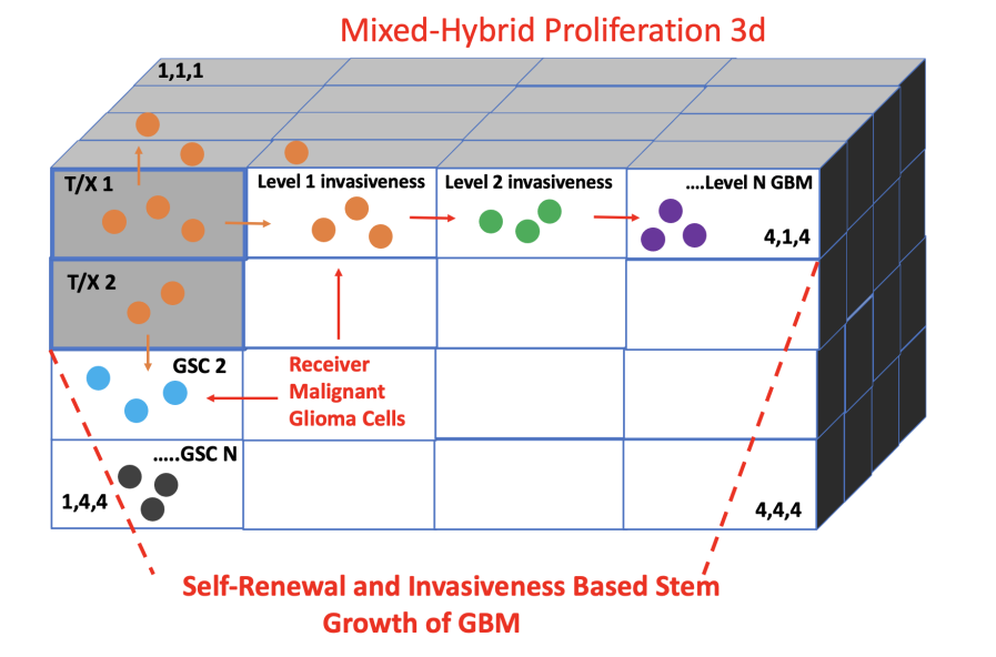
Figure 3: 3-dimensional voxel model Hybrid Configuration

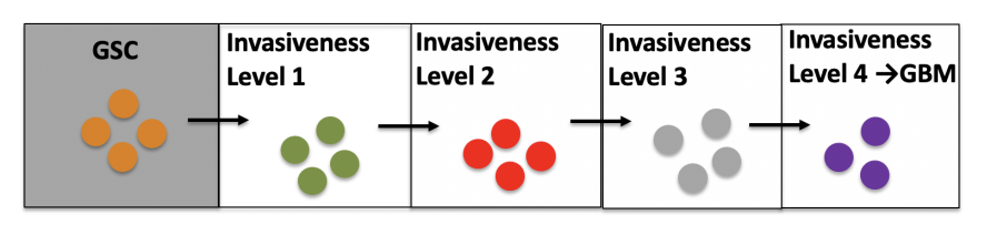
Figure 4: Series Voxel Model of Go Configuration

II-B Diffusion Reaction System

II-B1 Diffusion Subsystem

For this paper assume a general 3-d propagation medium of size $M_{x}\times M_{y}\times M_{z}$ cubic voxels. Each cubic voxel is assumed to represent a single transmitter or receiver cell. Figure 2 shows a 3-d dimensional hybrid configuration of malignant glioma, or glioblastoma, cells with $M_{x}=M_{y}=M_{z}=4$. For the ease of understanding we explain a simple example of voxel model in Figure 3 which depicts the Go (invasiveness) configuration of cells i.e. $M_{x}=5$ and $M_{y}=1$ and $M_{z}$ = 1. For this model, we obtain $n_{P,i}$ i.e. the number of input molecules $P$ in voxel $i$ as:

$$n_{P}(t)=[n_{P,1}(t),n_{P,2}(t),n_{P,3}(t),n_{P,4}(t)]^{T}$$ (1)

The terms on the R.H.S of Eq. (1) are updated with each new diffusion event. For example for the diffusion of a single molecule from transmitter cell-1 to receiver malignant glioma cell, the term $n_{P,1}(t)$ decreases by 1 whereas the term $n_{P,2}(t)$ increases by $1$. This is explained by using a jump vector $q_{d,1}(t)=[-1,1,0,0]^{T}$. The new state of the system after this diffusion event becomes $n_{P}(t)+q_{d,1}$. Additionally the term $W_{d,1}(n_{P}(t))=dn_{P,1}$ represents the jump rate function for this diffusion event. By combining all these jump vectors and the corresponding jump rate functions corresponding to each diffusion event we obtain a diffusion matrix $H$ as in [9]:

$$H=\left[\begin{array}[]{ccccc}-d&0&0&0\\ d&-d&0&0\\ 0&d&-d&0\\ 0&0&0&d\\ \end{array}\right]$$ (6)

where $-d$ indicates diffusion out of a voxel. The size of matrix $H$ depends on the number of interacting cells in the system. Next we use a SDE to model all the diffusion events [12]:

$$\dot{n}_{P}(t)=\sum_{j=1}^{J_{d}}q_{d,j}W_{d,j}(n_{P}(t))+\sum_{j=1}^{J_{d}}q_{d,j}\sqrt{W_{d,j}(n_{P}(t))}\gamma_{j}$$

$$+{\mathds{1}}_{T}U(t).$$ (7)

Eq. (7) is therefore a form of a chemical Langevin equation where the term $\sum_{j=1}^{J_{d}}q_{d,j}W_{d,j}(n_{P}(t))$ accounts for the deterministic dynamics of the system and $\gamma_{j}$ represents continuous-time Gaussian white noise. If all the jump rates are assumed as linear this leads to:

$$Hn_{P}(t) =\sum_{j=1}^{J_{d}}q_{d,j}W_{d,j}(n_{P}(t)).$$ (8)

The term $\sum_{j=1}^{J_{d}}q_{d,j}W_{d,j}\sqrt{W_{d,j}(n_{P}(t))}$ accounts for the the stochastic dynamics of the system. The term ${\mathds{1}}_{T}U(t)$ represents the transmitter input, i.e. emission rate.

II-B2 Reaction Subsystem

To derive the SDE for the reaction sub-system we assume that a ligand-binding type reaction takes place at each step of the node-stem structure of cells. In first reaction (5) the input molecules $P$ released from transmitter malignant glioma cell T/X-1 propagate to level 1 invasive receiver cell to produce output molecules $X_{[1]}$. These $X_{[1]}$ molecules act as the input in the next reaction (6) resulting in production of level 2 invasiveness $X_{[2]}$ molecules. This process process continues up to cell $N$ resulting in Level $N$ GBM.

(9)

(10)

Where $n_{P,R}$ represents the number of input molecules in the receiver glioma cell $i$ and $n_{X_{i}}$ represent the number of output molecules in receiver glioma cell $i$. The symbols $k_{0}$ - $k_{N}$ are the respective reaction rate constants. In Eq. (9) the input molecules $P$ react at the rate ${k}_{1}n_{P,R}$ producing output molecules $X_{[1]}$. For the sake of simplicity we derive the SDE for the case when we have only one receiver reaction i.e.Eq. (9). The input and output for this case is $n_{P,R}$ and $n_{X_{1}}$ respectively. We obtain the state vector as:

$$\tilde{n}_{R}(t) =\left[\begin{array}[]{c|c}n_{P,R}(t)&n_{X_{1}}(t)\end{array}\right]^{T}$$ (12)

and the corresponding SDE is given as:

$$\dot{\tilde{n}}_{R}(t) ={\rm I\!R}\tilde{n}_{R}(t)+\sum_{j=J_{d}+1}^{J_{d}+J_{r}}q_{r,j}\sqrt{W_{r,j}(\langle\tilde{n}_{R}(t)\rangle)}\gamma_{j}.$$ (13)

where $q_{r,j}$ and $W_{r,j}$ represent jump rates and jump vectors for the reaction events. The term $J_{d}$+ $J_{r}$ represents the total number of events (diffusion and reactions). ${\rm I\!R}$ is 2$\times$2 matrix with entries depending on reaction (9) see Table 1.

TABLE I: ${\rm I\!R}$ Matrix for receiver Reactions

Receiver	${\rm I\!R}$ Matrix
Reversible Reaction 5	$\begin{bmatrix}-k_{1}&k_{0}\\ k_{1}&-k_{0}\end{bmatrix}$

III End to End Model

To obtain the stochastic differential equation for the end to end model we combine the SDEs for diffusion-only and reaction-only subsystems. In this paper we have separately derived SDE’s for each subsystem in order to study the interconnection of both the subsystems. As the term $n_{P,R}(t)$ is common in the expressions for both $n_{P}(t)$ and $\tilde{n}_{R}(t)$ as shown in Eq.s (3) and (9), we consider it as the interconnection point between the two subsystems. For diffusion subsystem in Figure 3, the dynamics of number of signaling molecules in the receiver malignant glioma cell is given as:

$$\dot{n}_{P,R}(t)=dn_{P,T}(t)-dn_{P,R}(t)$$

$$+\underbrace{\sum_{j=1}^{J_{d}}[q_{d,j}]_{R}\sqrt{W_{d,j}(n_{P}(t))}\gamma_{j}}_{\xi_{d}(t)}$$ (16)

where $n_{P,T}$ represents the number of input molecules diffusing in the receiver. $[q_{d,j}]_{R}$ represents $R$-th element of jump vector $q_{d,j}$. Similarly for receiver subsystem, the dynamics of the input signalling molecules as a result of reaction (5) is given by the first element of Eq. (13), i.e.:

$$\dot{n}_{P,R}(t)=R_{11}n_{P,R}(t)+R_{12}n_{X_{1}}(t)$$

$$+\underbrace{\sum_{j=J_{d}+1}^{J_{d}+J_{r}}[q_{r,j}]_{1}\sqrt{W_{r,j}(\tilde{n}_{R}(t))}\gamma_{j}}_{\xi_{r}(t)}$$ (17)

where $[q_{r,j}]_{1}$ is the first element of jump vector $q_{r,j}$. We can then obtain the SDE for the end to end system by combining separate SDE’s derived in Eqs. (16) and (17): This shows that we can obtain SDE for the end to end system is obtained by combining SDE’s derived in Eq.s (3) and (9)) as:

$$\dot{n}(t) =An(t)+\sum_{j=1}^{J}q_{j}\sqrt{W_{j}(\langle n(t)\rangle)}\gamma_{j}+{\mathds{1}}_{T}U(t).$$ (18)

where $\langle n(t)\rangle$ (i.e. the mean of $n(t)$) is the solution to the following ODE:

$$\dot{\langle n(t)\rangle} =A\langle n(t)\rangle+{\mathds{1}}_{T}c$$ (19)

We can obtain the number of input molecules in the receiver (by taking Laplace of Eq. (18)) as:

$$N(s)=\underbrace{(sI-A)^{-1}{\mathds{1}}_{T}}_{\Psi(s)}U(s).$$ (20)

Multiplying this expression with $1_{X_{1}}$ we obtain the number of output molecules in receiver cell-1:

$$N_{X_{1}}(s)=1_{X_{1}}\underbrace{(sI-A)^{-1}{\mathds{1}}_{T}}_{\Psi(s)}U(s)$$ (21)

IV Communication Properties of System

IV-A Mutual Information

To derive expression for mutual information between the general input rate of molecules $U_{i}(t)$ and the general number of output molecules $n_{X_{i}}(t)$ i.e. $I(n_{X_{i}},U_{i})$ (where $i=1,2,..n$ number of transmitters or receivers) we use an expression for two Gaussian distribution random processes from [13]:

$$I(n_{X_{i}},U_{i}) =\frac{-1}{4\pi}\int_{-\infty}^{\infty}\log\left(1-\frac{|\Phi_{n_{X_{i}}U_{i}}(\omega)|^{2}}{\Phi_{n_{X_{i}}n_{X_{i}}}(\omega)\Phi_{U_{i}U_{i}}(\omega)}\right)d\omega$$ (22)

where $\Phi_{n_{X_{i}}n_{X_{i}}}(\omega)$ (resp. $\Phi_{U_{i}U_{i}}(\omega)$) represent the power spectral density of $n_{X_{i}}(t)$ ($U(t)$), and $\Phi_{n_{X_{i}}U_{i}}(\omega)$ is the cross spectral density of $n_{X_{i}}(t)$ and $U_{i}(t)$. From [14] we learn that that if all the jump rates $W_{j}(n(t))$ are linear in $n(t)$, then the power spectral density of $n(t)$ can be obtained by using Eq. (20). We can therefore describe the dynamics of the system in Eq. (18) by a set of linear SDE’s with $U_{i}(t)$ as the general input and $n_{X_{i}}(t)$ as the output. $\gamma_{j}$ in Eq. (18) accounts for the noise in the output. Therefore, Eq. (18) models a continuous-time linear time-invariant (LTI) stochastic system subject to a Gaussian input and Gaussian noise. We can then obtain the power spectral density $\Phi_{n_{X_{i}}}(\omega)$ as:

$$\Phi_{n_{X_{i}}}(\omega) =|\Psi(\omega)|^{2}\Phi_{U_{i}}(\omega)+\Phi_{\eta}(\omega)$$ (23)

where $\Phi_{U_{i}}(\omega)$ is the power spectral density of input $U_{i}(t)$ and $|\Psi(\omega)|^{2}$ is channel gain with $\Psi(\omega)=\Psi(s)|_{s=i\omega}$ defined as:

$${\color[rgb]{0,0,0}\Psi(s)={\mathds{1}}_{X_{i}}(sI-A)^{-1}{\mathds{1}}_{T}}$$ (24)

which is obtained by mean and Laplace of Eq. (18). $\Phi_{\eta}(\omega)$ represents the stationary noise spectrum:

$$\Phi_{\eta}(\omega) =\sum_{j=1}^{J_{d}+J_{r}}|{\mathds{1}}_{X_{1}}(i\omega I-A)^{-1}q_{j}|^{2}W_{j}(\langle n(\infty)\rangle)$$ (25)

where $\langle n(\infty)\rangle$ is the mean state of the system at time $\infty$ due to a constant input $c$. By using standard results for LTI system we obtain the cross spectral density $\Phi_{n_{X_{i}}U_{i}}(\omega)$ as:

$$|\Phi_{n_{X_{1}}U}(\omega)|^{2} =|\Psi(\omega)|^{2}\Phi_{U}(\omega)^{2}.$$ (26)

The final expression for mutual information $I(n_{{X_{i}}},U_{i})$ is obtained by substituting Eqs. (23) and  (26) in Eq. (22) as:

$$I(n_{{X_{i}}},U_{i})=\frac{1}{2}\int\log\left(1+\frac{|\Psi(\omega)|^{2}}{\Phi_{\eta}(\omega)}\Phi_{U_{i}}(\omega)\right)d\omega.$$ (27)

Maximum mutual information can be obtained by applying the water-filling solution to Eq. (27).

IV-B Information Propagation Speed

To compute the information propagation speed for multiple number of transmitter and receiver malignant glioma (or GBM) cells in different configurations we use the results of mutual information. For this we use the results of mutual information of the system for varying number of transmitters and receivers by using the expressions similar to Eq. (27). Next, by selecting a suitable threshold value of mutual information, we calculate the time difference when mutual information curve for various cases cross this threshold value. Finally, we calculate the information propagation speed $V$ by using the following expression:

$$V=\frac{1}{\mathbf{E}[\Delta t_{i,i+1}]}$$ (28)

where $\mathbf{E}$ is expectation operator and $\Delta t_{i,i+1}$ represents the time difference at which the mutual information for each case crosses the threshold.

IV-C Mathematical Model for tumour Growth

The GBM tumour growth relies on the cell proliferation probability $p(D)$ and accounts for both self-replicating and invading invasive malignant glioma cells. To compute the growth of tumour we use the expressions derived in [7] where the key variables controlling GBM growth are: the initial tumour growth rate $\lambda(0)$, the tumour growth rate over time $\lambda(t)$, the vascular growth retardation factor $\theta$ and the volume of growing tumour $V_{T}(t)$ (proportional to the number of receiver cells producing output molecules). The tumour volume increases according to the following ODE’s:

$$\frac{dV_{T}}{dt}=\lambda(t)V_{T}\approx n_{{X_{i}}}(t)V_{T}$$ (29)

$$\frac{d\lambda}{dt}=-\theta\lambda(0)\lambda.$$ (30)

where $V_{T}$ represents the volume of tumour depending on the cell proliferation probability. With the variations in the inter-cellular communication leading to the increasing flow of information molecules the GBM tumour volume increases. In particular, the tumour growth rate $\lambda(t)$ depends directly on the output of molecular communication system $n_{{X_{i}}}(t)$. $\theta$ $\leq$ 1 represents the retardation factor of the vascular structure.

V Numerical Results and Discussions

In this section we present numerical results for different configurations and multiple malignant glioma transmitter and receiver cells on the structure of GBM growth. Some of the main parameters considered in this work are based on previous work [7]. The propagation medium is assumed as rectangular prism which is divided into a number of cubic voxels. For example if we assume a a propagation medium of size 1$\frac{2}{3}\mu$m$\times$1$\frac{2}{3}\mu$m$\times$1$\frac{2}{3}\mu$m where each voxel has a size $\frac{1}{3}$ $\mu$m³ this will lead to rectangular prism of $5\times 5\times 5$ voxels. Using this general methodology we can vary the propagation medium sizes for different system settings such as the number of cells or input molecules. For neural cells considered in this paper we consider size = 20 $\mu$m [15]. We further assume diffusion coefficient $D$ = 1 $\mu$m²s^-1 for the propagation medium. The reaction rate constants are $k_{1}$ = $k_{0}$ = 1. For each cell we assume six neighbouring cells as in 3-d voxel model with the distance between cells as 1-5 $\mu$ m. The radius of the propagation environment is 4 mm and cell proliferation probability $p(D)$ is assumed to be 1. The tumour growth retardation factor $\theta$ is 0.53-0.99 whereas the tumour doubling time is $0.693/\lambda$. For the results presented in this section we assume absorbing boundary condition such that molecules can escape the medium at rate $\frac{d}{50}$. The value of deterministic emission rate $c$ is chosen such that it derives the transformation of transmitter GSC cell into a tumour cell. Our main aim is to explore the impact of multiple transmitter cells on the mutual information and hence the structure of GBM tumour growth for varying number of transmitter and receiver cells in different configurations. The main results obtained in this paper are as follows. First in Figure 5 we present the results for growth rate of tumour which proliferates by receiving input information carrying molecules emitted by the transmitter. We show that with the increase in the number of input molecules the growth of tumour at time $t$ also increases. However we observe that the growth is higher in hybrid configuration.

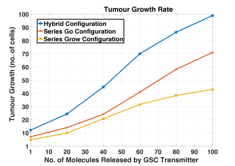
Figure 5: Tumour Growth rate (number of cells) vs No. of molecules

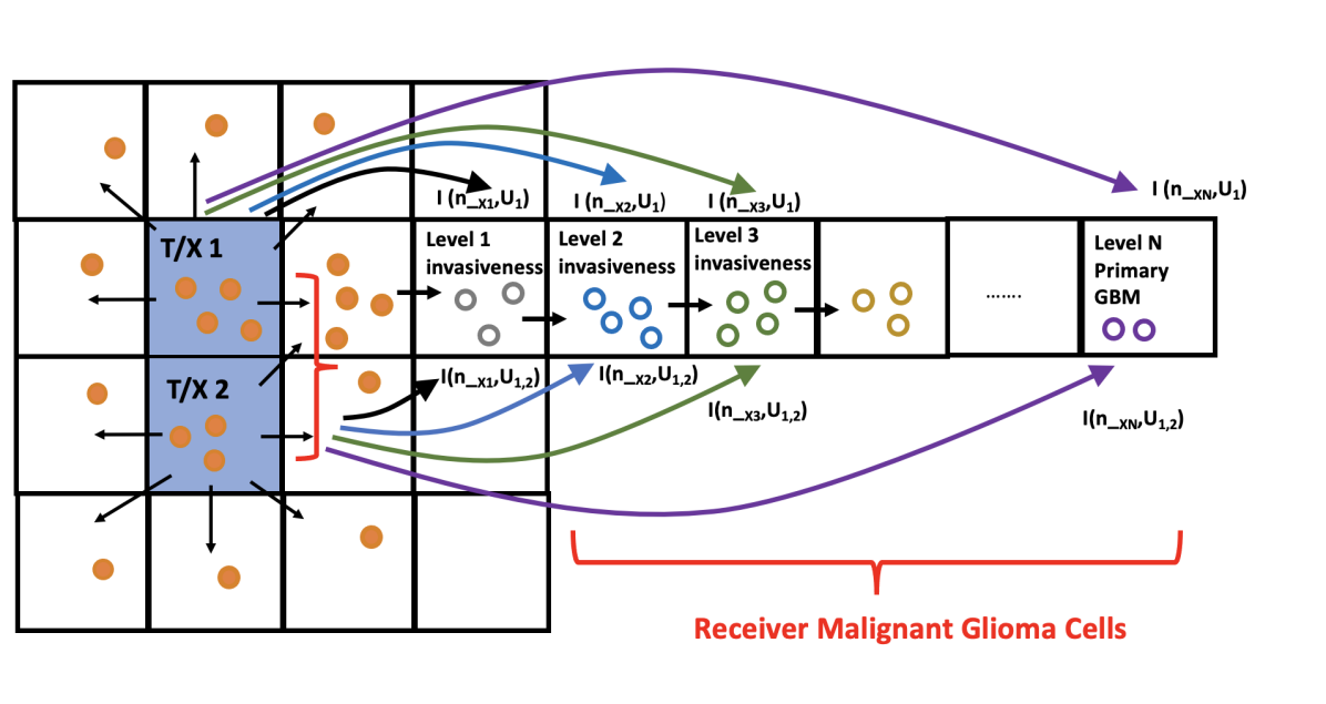
Figure 6: Mutual information Comparison Scenarios- Go

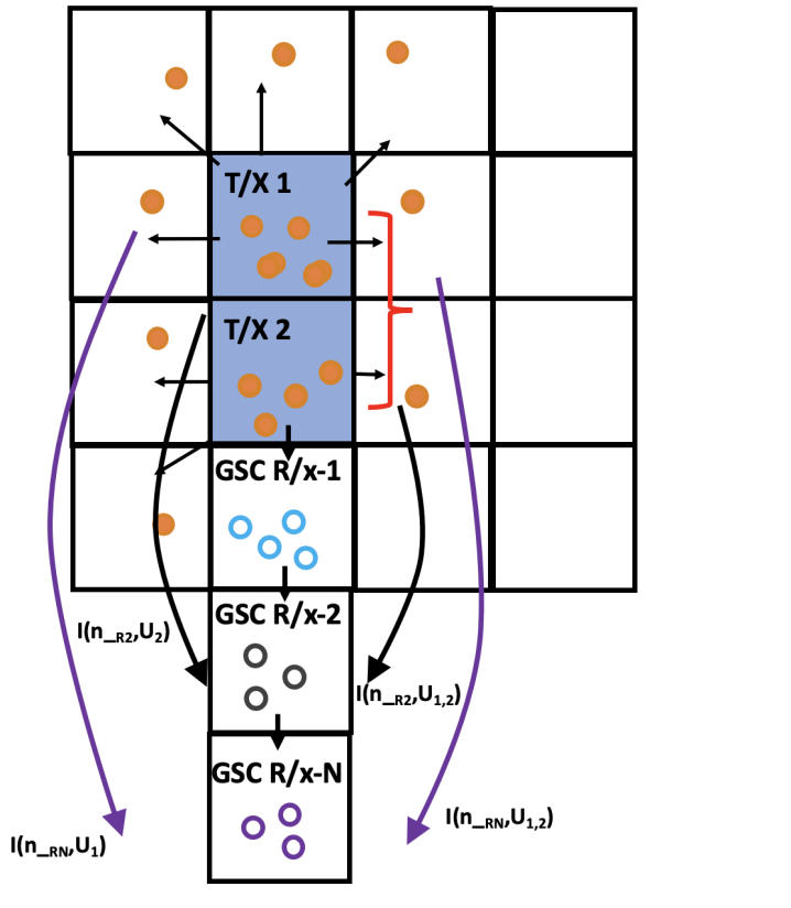
Figure 7: Mutual information Comparison Scenarios- Grow

In Figures 6 and 7 we present various comparison scenarios for mutual information of single and multiple transmitter glioma stem cells in both Grow and Go configurations for an increasing number of receiver malignant glioma cells. As shown in Figures 8 and 9 the total mutual information (for both Go and Grow) tends to increase as the number of both transmitters and receiver malignant glioma cells increase. This is due to the reduction in noise as a result of increased capture of molecules by receivers. This result also suggests that a higher mutual information among glioma cells in a particular direction will result in higher GBM growth rate (stem growth) in that direction as shown in Figure 1.

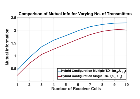
Figure 8: Mutual information-Single vs Multiple Transmitter- Go

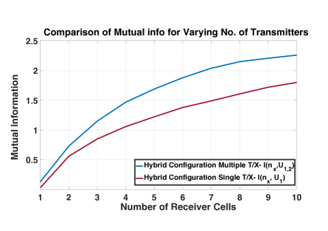
Figure 9: Mutual information-Single vs Multiple Transmitter- Grow

Finally in Figure 10 we present a comparison for information propagation between node and stem cells of GBM (as shown in Figure 1). We learn that due to lower density of cells in the stem the information propagation speed is higher in stem as compared to node. However, we note that that due to lower density of cells in stem this area can be targeted by potential therapeutic mechanisms for GBM.

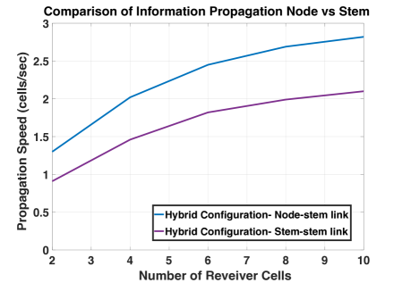
Figure 10: Information propagation speed comparison- Node vs Stem

VI Conclusion

This paper is focused on understanding the mechanisms by which a network of multiple bio-nanomachines (transmitters and receivers) in a molecular communication system influence the growth structure of GBM tumour, a grade IV malignant glioma. By using a voxel model for multiple transmitter and receiver cells, this paper provides new insights into the role of inter-cellular communication (i.e. the mutual information between cells) in the evolution and progression of GBM (stem from node). From the results of this paper we learn that the growth of tumour in any particular direction is driven by the increase in the mutual information between multiple cells in the node-stem structure. We further learn that information propagation speed between cells can vary at different points in the node and stem. This knowledge can be useful for developing future therapeutic mechanisms targeting GBM.

References

- [1] I. Akyildiz, M. Pierobon, S. Balasubramaniam, and Y. Koucheryavy, “The internet of bio-nano things,” IEEE Communications Magazine, vol. 53, no. 3, pp. 32–40, 2015.
- [2] M. Kuscu, E. Dinc, B. A. Bilgin, H. Ramezani, and O. B. Akan, “Transmitter and receiver architectures for molecular communications: A survey on physical design with modulation, coding, and detection techniques,” Proceedings of the IEEE, vol. 107, no. 7, pp. 1302–1341, 2019.
- [3] N. Farsad, A. W. Eckford, S. Hiyama, and Y. Moritani, “A simple mathematical model for information rate of active transport molecular communication,” in Computer Communications Workshops (INFOCOM WKSHPS), 2011 IEEE Conference on, pp. 473–478, IEEE, 2011.
- [4] C. T. Chou, “Molecular communication networks with general molecular circuit receivers,” in ACM The First Annual International Conference on Nanoscale Computing and Communication, (New York, New York, USA), pp. 1–9, ACM Press, 2014.
- [5] N. Jhaveri, T. C. Chen, and F. M. Hofman, “Tumor vasculature and glioma stem cells: Contributions to glioma progression,” Cancer Letters, vol. 380, no. 2, pp. 545–551, 2016.
- [6] M. Veletić, M. T. Barros, H. Arjmandi, S. Balasubramaniam, and I. Balasingham, “Modeling of modulated exosome release from differentiated induced neural stem cells for targeted drug delivery,” IEEE Transactions on NanoBioscience, vol. 19, no. 3, pp. 357–367, 2020.
- [7] H. Awan, S. Balasubramaniam, and A. Odysseos, “A voxel model to decipher the role of molecular communication in the growth of glioblastoma multiforme,” IEEE Transactions on NanoBioscience, pp. 1–1, 2021.
- [8] E. Jung, J. Alfonso, M. Osswald, H. Monyer, W. Wick, and F. Winkler, “Emerging intersections between neuroscience and glioma biology,” Nature Neuroscience, pp. 1–10, 2019.
- [9] H. Awan and C. T. Chou, “Molecular communications with molecular circuit-based transmitters and receivers,” IEEE transactions on nanobioscience, vol. 18, no. 2, pp. 146–155, 2019.
- [10] M. U. Riaz, A. Hamdan, and C. T. Chou, “Using spatial partitioning to reduce the bit error rate of diffusion-based molecular communications,” IEEE Transactions on Communications, vol. 68, no. 4, pp. 2204–2220, 2020.
- [11] H. Awan and C. T. Chou, “Demodulation of reaction shift keying signals in molecular communication network with protein kinase receiver circuit,” in 2016 IEEE Wireless Communications and Networking Conference (WCNC), pp. 1–6, IEEE, 2016.
- [12] C. Gardiner, Stochastic methods. Springer Berlin, 2009.
- [13] F. Tostevin and P. R. Ten Wolde, “Mutual information in time-varying biochemical systems,” Physical Review E, vol. 81, no. 6, p. 061917, 2010.
- [14] P. B. Warren, S. Tănase-Nicola, and P. R. ten Wolde, “Exact results for noise power spectra in linear biochemical reaction networks,” The Journal of chemical physics, vol. 125, no. 14, p. 144904, 2006.
- [15] W. Diao, X. Tong, C. Yang, F. Zhang, C. Bao, H. Chen, L. Liu, M. Li, F. Ye, Q. Fan, et al., “Behaviors of glioblastoma cells in in vitro microenvironments,” Scientific reports, vol. 9, no. 1, pp. 1–9, 2019.