The conformal Einstein field equations and the local extension of future null infinity

Abstract

We make use of an improved existence result for the characteristic initial value problem for the conformal Einstein equations to show that given initial data on two null hypersurfaces $\mathcal{N}_{\star}$ and $\mathcal{N}^{\prime}_{\star}$ such that the conformal factor (but not its gradient) vanishes on a section of $\mathcal{N}_{\star}$ one recovers a portion of null infinity. This result combined with the theory of the hyperboloidal initial value problem for the conformal Einstein field equations allows to show the semi-global stability of the Minkowski spacetime from characteristic initial data.

1 Introduction

This is the third article in a series devoted to the analysis of the characteristic initial value problem (CIVP) for the Einstein field equations. This research programme is motivated by the techniques introduced by Luk in [1] to obtain local existence results for the Einstein field equations which are optimal in the sense that one obtains a solution in a neighbourhood of both the initial null hypersurfaces and not only in a neighbourhood of their intersection as in Rendall’s original approach [2]. In Paper I of this series, see [3], we obtained an improved local existence result for the CIVP for the Einstein field equations expressed in terms of the Newman-Penrose formalism and a gauge due to Stewart —see [4]. This result demonstrates the robustness of Luk’s approach, showing that the specific choice of gauge employed in [1] is not crucial. In Paper II of this series, see [5], we applied Luk’s method to obtain a local existence result for the asymptotic CIVP for Friedrich’s conformal Einstein field equations. In this problem, one of the initial hypersurfaces is past null infinity while the other is an incoming light cone —in an alternative version of this problem one prescribes data on future null infinity and an outgoing null hypersurface.

The problem. In this article we make use of a CIVP for the conformal Einstein field equations to study the question of the local extendibility of null infinity. To this end, initial data is prescribed on two future oriented null hypersurfaces intersecting a 2-dimensional surface with the topology of the 2-sphere $\mathbb{S}^{2}$. These null hypersurfaces are assumed to intersect future null infinity, $\mathscr{I}^{+}$. The question to be addressed is whether it is possible to recover a portion of future null infinity lying in the causal future of the initial hypersurfaces. Observe that in the future null infinity version of the asymptotic CIVP analysed in Paper II, the solution constructed is located in the causal past of the initial hypersurfaces —see Figure 1. The question of the local extendibility of null infinity through a CIVP has been studied by Li & Zhu in [6] directly through the Einstein field equations. In this work, in order to encode the asymptotic behaviour of the various field at infinity it is necessary to make use of weighted function spaces and norms. Moreover, it is necessary to consider the existence of solutions to the field equations on a domain with an infinite extent. In this article we make use of an alternative setup that offers a natural way to address the local extendibility of null infinity: the use of a conformal representation of the spacetime and the conformal Einstein field equations —see e.g. [7].

Conformal methods. The use of conformal methods in the study of the local extendibility of (future) null infinity allows to transform the question of existence of solutions to hyperbolic evolution equations on an infinite domain into the study of solutions on a finite region. Moreover, the asymptotic decay of the various fields fields is conveniently encoded through regularity of the fields. Accordingly, it is possible to work with standard (unweighted) function spaces and norms. Luk’s strategy to analyse the CIVP allows to ensure the existence of solutions on causal diamonds having a long and a short direction —see Figure 1. Existence in the long direction is ensured as long as one has control on the initial data. On the other hand, the extent of the short direction is restricted by the potential appearance of singularities in finite time due to the presence of Riccati-type equations in the evolution system. In the present problem the conformal framework provides a natural causal diamond with one of its sides lying on one of the null initial hypersurfaces, $\mathcal{N}_{\star}$, and a short side covering a portion of null infinity. Although from the point of view of the conformal representation this domain has a finite size, in the physical spacetime it actually represents an infinite domain contained between two parallel null hypersurfaces. The main result of this article is that it is possible to ensure the existence of solutions to the conformal Einstein field equations on the causal diamond with sides on $\mathcal{N}_{\star}$ and $\mathscr{I}^{+}$. Thus, it is possible to recover a portion of null infinity to the future of $\mathcal{N}_{\star}$ —i.e. we have extended $\mathscr{I}^{+}$.

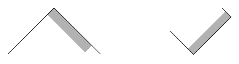
Figure 1: Comparison between the asymptotic characteristic problem (a) and the standard characteristic problem (b) for the conformal Einstein field equations. In the future null infinity version of the asymptotic CIVP initial data is prescribed on future null infinity and on an outgoing lightcone $\mathcal{N}_{\star}$. The neighbourhood theorem allows the recovery of a narrow causal diamond along null infinity. The length of this rectangle is limited by the portion of $\mathscr{I}^{+}$ on which one has control of the initial data. Observe that region of existence of solutions lies in the causal past of the null hypersurfaces and that the existence of, at least a portion of null infinity is a priori assumed. In the characteristic problem considered in this article the initial data is prescribed on two standard null hypersurfaces $\mathcal{N}_{\star}$ and $\mathcal{N}_{\star}^{\prime}$ with at least one of them ($\mathcal{N}_{\star}$) intersecting the conformal boundary. The improved existence result allows then to recover a narrow rectangle whose long side lies on $\mathcal{N}_{\star}$ and the short one gives a portion of future null infinity. Observe that the region of existence is on the causal future of the initial hypersurfaces and that, a priori only the existence of a cut of null infinity is assumed.

The hyperboloidal initial value problem. Historically, the first resolution of the local extendibility of null infinity has been given by Friedrich in his analysis of the hyperboloidal initial value problem for the conformal Einstein field equations —see [8, 9], also [10, 7]. In this case, initial data is prescribed on a spatial hypersurface $\mathcal{H}_{\star}$ which intersects null infinity. Due to the formal regularity of the conformal Einstein field equations at the conformal boundary, the standard local existence theory for symmetric hyperbolic systems allows to recover a slab of spacetime in the causal future of $\mathcal{H}_{\star}$ which covers a portion of null infinity —see Figure 2. A particular drawback of this approach, in contrast with the CIVP, is the increased complexity in solving the constraint equations on $\mathcal{H}_{\star}$ and obtaining conditions ensuring peeling (see below) —see [11, 12, 13]. In view of the latter and the historical and practical relevance of the CIVP it is of interest to discuss the extendibility of null infinity form this alternative point of view.

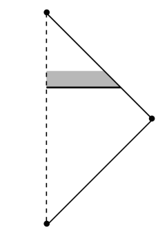
Figure 2: A schematic depiction of a hyperboloidal IVP in an asymptotically flat spacetime. Suitable initial data is given on $\mathcal{H}_{\star}$, and local existence is guaranteed in the (local) shaded region provided regularity and symmetric hyperbolicity of the equations of motion under consideration.

Peeling. The problem here considered is closely related to one of the central issues on the study of the asymptotics of the gravitational field: peeling. As part of the formulation of the CIVP here considered it is necessary to prescribe the value of one of the components of the Weyl tensor ($\phi_{0}$) on one of the null hypersurfaces. This component is usually loosely interpreted as describing some sort of incoming radiation —see [14]. For simplicity, in the present analysis it is assumed that the component $\phi_{0}$ is smooth at null infinity. It follows that on the portion of future null infinity recovered by the optimal local existence result for the CIVP the Weyl tensor satisfies the peeling behaviour. If a finite regularity is assumed below a certain threshold, then the assumptions of the peeling theorem are no longer satisfied —see e.g. [15, 4, 7].

Differences with the asymptotic characteristic problem. The CIVP considered in this article differs from that in Paper II in that in the former one of the initial hypersurfaces coincides with the conformal boundary. This leads to a number of simplifications in the gauge and equations. In the present case, both initial null hypersurfaces lie in the physical spacetime —except for their intersections with null infinity. Thus, one has to deal with a somewhat more general set up. Nevertheless, a careful inspection of the analysis of Paper II shows that all the main assertions and estimates hold in the present situation. Roughly speaking these estimates control the size of the $L^{2}$-norm of the fields appearing in the conformal Einstein field equations in terms of the size of the initial data. Thus, if the data is finite, so will also the solutions to the conformal Einstein field equations. The existence of solutions on the causal diamond containing a portion of null infinity then follows from a last slice argument in which the basic existence domain arising from the use of Rendall’s reduction strategy [2] is progressively extended.

An application: the semi-global stability of Minkowski spacetime from a Cauchy-characteristic problem. As an application of our result on the local extendibility of null infinity in the CIVP for the conformal Einstein field equations, we obtain a semi-global stability result for the Minkowski spacetime. The idea behind this construction is the following: given standard Cauchy initial data for the conformal Einstein field equations on a compact spacelike domain $\mathcal{K}_{\star}$, and characteristic data up to the conformal boundary on an outgoing null hypersurface $\mathcal{N}_{\star}$ emanating from the boundary of the spacelike domain the development of Cauchy data implies complementary characteristic data on the Cauchy horizon $H^{+}(\mathcal{K}_{\star})$ of the development. In turn, setting $\mathcal{N}_{\star}=H^{+}(\mathcal{K}_{\star})$, the local extendibility result of null infinity can be used to obtain two (intersecting) causal diamonds along the initial null hypersurfaces $\mathcal{N}_{\star}$ and $\mathcal{N}_{\star}^{\prime}$ both including a portion of future null infinity. Accordingly, the existence domain along the initial hypersurface $\mathcal{K}_{\star}\cup\mathcal{N}_{\star}$ will contain a hyperboloidal hypersurface $\mathcal{H}_{\star}$. If the initial data on $\mathcal{K}_{\star}\cup\mathcal{N}_{\star}$ is assumed to be suitably close to data for the Minkowski spacetime, then the initial data induced on $\mathcal{H}_{\star}$ will also be close to Minkowski hyperboloidal data. One can then use Friedrich’s semi-global existence stability results in [9] —see also [10]— to recover the whole of the domain of dependence $D^{+}(\mathcal{K}_{\star}\cup\mathcal{N}_{\star})$. For a recent alternative proof of the stability of the Minkowski spacetime from Cauchy-characteristic data which makes use of the full machinery of vector field methods —see [16].

Conventions

This article follows the conventions and notation of Paper I and Paper II, which, in turn follow those used in the monograph [7]. The latter reference is consistent with the presentation in J. Stewart’s book [4] and Penrose & Rindler [17, 15].

2 The conformal vacuum Einstein field equations

The main technical tool for the analysis of the the local extension of future null infinity are Friedrich’s conformal vacuum Einstein field equations (CEFE). The equations are a conformal representation of the vacuum Einstein field equations. Crucially, they are formally regular on the conformal boundary and imply, away from it, a solution to the vacuum Einstein field equations. The structural properties of the CEFE and its derivation have been amply discussed in the literature —see [8, 7].

In what follows, let ($\mathcal{M},{\bm{g}},\Xi$) denote a conformal extension of a vacuum asymptotically simple spacetime (see [15, 7] for a definition) $(\tilde{\mathcal{M}}$, $\tilde{{\bm{g}}}$. The physical metric $\tilde{\bm{g}}$ and the unphysical metric ${\bm{g}}$ are related to each other via the formula ${\bm{g}}=\Xi^{2}\tilde{{\bm{g}}}$. By assumption, the unphysical manifold $\mathcal{M}$ has a boundary —the conformal boundary, $\mathscr{I}\equiv\partial\mathcal{M}$, corresponding to the future endpoints of null geodesics. The conformal factor satisfies $\Xi>0$ on $\mathcal{M}\setminus\mathscr{I}$ and $\Xi=0$, ${\bm{d}}\Xi\neq 0$ on $\mathscr{I}$ —that is, $\Xi$ is a boundary defining function.

The metric vacuum conformal Einstein field equations with vanishing Cosmological constant are given by the system

$$\nabla_{a}\nabla_{b}\Xi=-\Xi L_{ab}+sg_{ab},$$ (1a)

$$\nabla_{a}s=-L_{ac}\nabla^{c}\Xi,$$ (1b)

$$\nabla_{c}L_{db}-\nabla_{d}L_{cb}=\nabla_{a}\Xi d^{a}{}_{bcd},$$ (1c)

$$\nabla_{a}d^{a}{}_{bcd}=0,$$ (1d)

$$6\Xi s-3\nabla_{c}\Xi\nabla^{c}\Xi=0,$$ (1e)

$$R^{c}{}_{dab}=C^{c}{}_{dab}+2\big{(}\delta^{c}{}_{[a}L_{b]d}-g_{d[a}L_{b]}{}^{c}\big{)},$$ (1f)

where

$$L_{ab}\equiv\frac{1}{2}R_{ab}-\frac{1}{12}Rg_{ab},\qquad d^{a}_{\phantom{a}bcd}\equiv\Xi^{-1}C^{a}_{\phantom{a}bcd},\qquad s\equiv\frac{1}{4}\nabla^{a}\nabla_{a}\Xi+\frac{1}{24}R\Xi,$$

are, respectively, the Schouten tensor, the rescaled Weyl tensor and the Friedrich scalar. For convenience we also define

$$\Sigma_{a}\equiv\nabla_{a}\Xi.$$

The analysis of this article will be carried out with a Newman-Penrose (NP) version of the above equations in which the various tensor field and equations are expressed in terms of a null (NP) tetrad. The detailed form of these equations can be found in the Appendix of Paper II.

3 The geometry of the problem

In this section we discuss the geometric setting of the local extension of future null infinity. This is very similar to the one used in Papers I and II and makes use of a gauge which we will call Stewart’s gauge. The reader is referred to [3, 5] for further details and discussion —see also [18, 4].

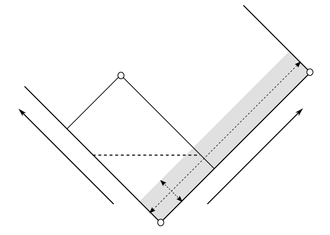
Figure 3: Geometric setup for the analysis of the local extension of future null infinity. The construction makes use of a double null foliation of the domain of dependence of the initial hypersurface $\mathcal{N}^{\prime}_{\star}\cup\mathcal{N}_{\star}$. The null hypersurface $\mathcal{N}_{\star}$ terminates at the conformal boundary where $\Xi=0$. Our construction allows us to recover a portion of length $\epsilon$ on $\mathscr{I}^{+}$. The coordinates and null NP tetrad are adapted to this geometric setting. The analysis is focused on the thing grey rectangular domain along $\mathcal{N}_{\star}$. The conformal Einstein field equation allows to treat this problem on an infinite domain in terms of a problem in unphysical space on a finite domain.

3.1 Basic geometric setting

In our basic setting, the unphysical manifold $\mathcal{M}$ has a boundary and two edges. The boundary consists of three null hypersurfaces: the outgoing null hypersurface $\mathcal{N}_{\star}$; the incoming null hypersurface $\mathcal{N}_{\star}^{\prime}$ with non-vacuum intersection $\mathcal{S}_{\star}\equiv\mathcal{N}_{\star}\cap\mathcal{N}_{\star}^{\prime}$; future null infinity $\mathscr{I}^{+}$ intersecting with $\mathcal{N}_{\star}$ at the corner $\mathcal{S}^{\prime}_{\star}$. For concreteness, we will assume that $\mathcal{S}_{\star},\mathcal{S}^{\prime}_{\star}\approx\mathbb{S}^{2}$. See Figure 3 for further details.

One can introduce coordinates $\bar{x}=(x^{\mu})$ in a neighbourhood $\mathcal{U}$ of $\mathcal{Z}_{\star}$ with $x^{0}=v$ and $x^{1}=u$ such that, at least in a neighbourhood of $\mathcal{S}_{\star}$ one can write

$$\mathcal{N}_{\star}=\{p\in\mathcal{U}\mid u(p)=0\},\qquad\mathcal{N}_{\star}^{\prime}=\{p\in\mathcal{U}\mid v(p)=0\}.$$

Given suitable data on $(\mathcal{N}_{\star}\cap\mathcal{N}_{\star}^{\prime})\cap\mathcal{U}$ we are interested in making statements about the existence and uniqueness of solutions to the CEFE on some open set

$$\mathcal{V}\subset\{p\in\mathcal{U}\mid u(p)\geq 0,v(p)\geq 0\}$$

which we identify with a subset of the future domain of dependence, $D^{+}(\mathcal{N}_{\star}\cup\mathcal{N}_{\star}^{\prime})$ of $\mathcal{N}_{\star}\cup\mathcal{N}_{\star}^{\prime}$. Moreover, we want to show that the existence region can be extended along $\mathcal{N}_{\star}$ to reach the conformal conformal boundary —this improved existence domain corresponds to the grey rectangle in Figure 3.

3.2 Stewart’s Gauge

Following the discussion of Papers I and II, in the following we assume that the future of $\mathcal{S}_{\star}$ can be foliated by a family of null hypersurfaces: $\mathcal{N}_{u}$ (the outgoing null hypersurfaces) and $\mathcal{N}_{v}^{\prime}$ (the ingoing null hypersurfaces). The scalars $u$ and $v$ each satisfy the eikonal equation

$${\bm{g}}^{\sharp}(\mathbf{d}u,\mathbf{d}u)={\bm{g}}^{\sharp}(\mathbf{d}v,\mathbf{d}v)=0.$$

In particular, we assume that $\mathcal{N}_{0}=\mathcal{N}_{\star}$ and $\mathcal{N}_{0}^{\prime}=\mathcal{N}_{\star}^{\prime}$. Following standard usage, we call $u$ a retarded time and $v$ an advanced time and use these two scalar fields $u$ and $v$ as coordinates in a neighbourhood of $\mathcal{S}_{\star}$. To complete the coordinate system, consider arbitrary coordinates $(x^{\mathcal{A}})$ on $\mathcal{D}_{\star}$, with the index ^A taking the values $2,\,3$. These coordinates are then propagated into $\mathcal{N}_{\star}$ by requiring them to be constant along the generators of $\mathcal{N}_{\star}$. Once coordinates have been defined on $\mathcal{N}_{\star}$, one can propagate them into $\mathcal{V}$ by requiring them to be constant along the generators of each $\mathcal{N}_{v}^{\prime}$. In this manner one obtains a coordinate system $(x^{\mu})=(u,\,v,\,x^{\mathcal{A}})$ in $\mathcal{V}$. Moreover, we define $\mathcal{S}_{u,v}\equiv\mathcal{N}_{u}\cap\mathcal{N}_{v}^{\prime}\approx\mathbb{S}^{2}$. Our analysis will be mostly carried out in causal diamonds of the form

$$\mathcal{D}_{u^{\prime},v^{\prime}}\equiv\{0\leq v\leq v^{\prime},\;0\leq u\leq u^{\prime}\}=\cup_{0\leq v\leq v^{\prime},0\leq u\leq u^{\prime}}\mathcal{S}_{u,v}.$$

By means of the time function $t\equiv u+v$ one can readily define the truncated causal diamond

$$\mathcal{D}^{\tilde{t}}_{u^{\prime},v^{\prime}}\equiv\mathcal{D}_{u^{\prime},v^{\prime}}\cap\{t\leq\tilde{t}\}.$$

The above coordinate construction is complemented by an NP null tetrad $\{{\bm{l}},\,{\bm{n}},\,{\bm{m}},\,\bar{\bm{m}}\}$ with the vectors ${\bm{l}}$ and ${\bm{n}}$ tangent to the generators of the null hypersurfaces $\mathcal{N}_{u}$ and $\mathcal{N}_{v}^{\prime}$ respectively. Following the same discussion of Papers I and II we make

Gauge choice 1 (Stewart’s choice of the components of the frame).

On $\mathcal{V}$ we consider a NP frame of the form

$${\bm{l}}={\bm{\partial}}_{v}+C^{\mathcal{A}}{\bm{\partial}}_{\mathcal{A}},\ \ {\bm{n}}=Q{\bm{\partial}}_{u},\ \ {\bm{m}}=P^{\mathcal{A}}{\bm{\partial}}_{\mathcal{A}},$$ (2)

where $C^{\mathcal{A}}=0$ on $\mathcal{N}_{\star}$, ${\bm{m}}$ and $\bar{\bm{m}}$ span the tangent space of $\mathcal{S}_{u,v}$. On $\mathcal{N}_{\star}^{\prime}$ one has that ${\bm{n}}=Q{\bm{\partial}}_{u}$. As the coordinates $(x^{\mathcal{A}})$ are constant along the generators of $\mathcal{N}_{\star}$ and $\mathcal{N}_{\star}^{\prime}$, it follows that on $\mathcal{N}_{\star}^{\prime}$ the coefficient $Q$ is only a function of $u$. Thus, without loss of generality one can re-parameterise $u$ so as to set $Q=1$ on $\mathcal{N}_{\star}^{\prime}$.

Direct inspection of the NP commutators applied to the coordinates $(u,\,v,\,x^{\mathcal{A}})$ leads to the following:

Lemma 1 (conditions on the connection coefficients).

The NP frame of the Gauge Choice 1 can be chosen such that

$$\kappa=\nu=\gamma=0,$$ (3a)

$$\rho=\bar{\rho},\ \ \mu=\bar{\mu},$$ (3b)

$$\pi=\alpha+\bar{\beta},$$ (3c)

on $\mathcal{V}$ and, furthermore, with

$$\epsilon-\bar{\epsilon}=0\ \ \ \textrm{on}\ \ \ \mathcal{V}\cap\mathcal{N}_{\star}.$$

Remark 1.

Additional commutator relations can be used to obtain equations for the frame coefficients $Q$, $P^{\mathcal{A}}$ and $C^{\mathcal{A}}$ —see equations (LABEL:PaperII-framecoefficient1)-(LABEL:PaperII-framecoefficient6) in Paper II.

In addition to the coordinate and frame gauge freedom we also need to fix the conformal gauge freedom. This is done in the following lemma whose proof follows the same scheme as Lemma LABEL:PaperII-Lemma:ConformalGauge in Paper II:

Lemma 2 (conformal gauge conditions for characteristic problem).

Let $(\tilde{\mathcal{M}},\tilde{{\bm{g}}})$ denote a vacuum asymptotically simple spacetime and let $(\mathcal{M},{\bm{g}},\Xi)$ with ${\bm{g}}=\Xi^{2}\tilde{{\bm{g}}}$ a conformal extension. Given the NP frame of the Gauge Choice 1, the conformal factor $\Xi$ can be chosen so that

$$\mathit{R}[{\bm{g}}]=R(x),\qquad\textrm{in a neighbourhood}\quad\mathcal{V}\quad\textrm{of}\quad\mathcal{S}_{\star}\quad\textrm{on}\quad J^{+}(\mathcal{S}_{\star})$$

where $R(x)$ is an arbitrary function of the coordinates. Moreover, one has the additional gauge conditions

$$\Sigma_{2}=1,\ \ \ \ \textrm{on}\ \ \mathcal{S}_{\star},$$

$$\Phi_{22}=0\ \ \ \ \textrm{on}\ \ \mathcal{N}^{\prime}_{\star},$$

$$\Phi_{00}=0\ \ \ \ \textrm{on}\ \ \mathcal{N}_{\star}.$$

4 The formulation of the characteristic initial value problem

This section provides a brief discussion of the basic set up and local existence theory of the CIVP for the conformal Einstein field equations with data on the null hypersurfaces $\mathcal{N}_{\star}$ and $\mathcal{N}_{\star}^{\prime}$ using Rendall’s reduction strategy [2] —see also Section 12.5 of [7]. The analysis is completely analogous to the one carried out in Paper I in which the initial value problem for the vacuum Einstein field equations was considered —note, by contrast, the conceptual difference with Paper II in which an asymptotic characteristic problem was considered.

4.1 Specifiable free data

In order to obtain a solution in the domain $J^{+}(\mathcal{S}_{\star})$, we need to provide initial data for the evolution equations on $\mathcal{N}_{\star}\cup\mathcal{N}_{\star}^{\prime}$. In particular, we need to know the value of the derivatives of conformal factor $\{\Sigma_{1},\ \Sigma_{2},\ \Sigma_{3},\ \Sigma_{4}\}$, the components of frame $\{C^{\mathcal{A}},\ P^{\mathcal{A}},Q\}$, the spin connection coefficients $\{\epsilon,\ \pi,\ \beta,\ \mu,\ \alpha,\ \lambda,\ \tau,\ \sigma,\ \rho\}$, the rescaled Weyl tensor $\{\phi_{0},\ \phi_{1},\ \phi_{2},\ \phi_{3},\ \phi_{4}\}$ and the Ricci tensor $\{\Phi_{00},\ \Phi_{01},\ \Phi_{11},\ \Phi_{02},\ \Phi_{12},\ \Phi_{22}\}$ on the initial hypersurfaces. However, as a consequence of the constraints implied by the CEFE, this data cannot be freely specified. As in the case of the discussion in Papers I and II, The hierarchical structure of the CEFE allows to identify the basic reduced initial data set $r_{\star}$ from which the full initial data on $\mathcal{N}_{\star}\cup\mathcal{N}_{\star}^{\prime}$ for the conformal Einstein field equations can be computed. The following lemma shows us the freely specifiable data for our characteristic problem.

Lemma 3 (freely specifiable data for the characteristic problem).

Assume that the Gauge Choice 1 and the gauge conditions implied by Lemmas 1 and 2 are satisfied in a neighbourhood $\mathcal{V}$ of $\mathcal{S}_{\star}$. Initial data for the conformal Einstein field equations on $\mathcal{N}_{\star}\cup\mathcal{N}_{\star}^{\prime}$ can be computed from the reduced data set $\mathbf{r}_{\star}$ consisting of:

$$\phi_{0},\;\Xi,\quad\mbox{on}\quad\mathcal{N}_{\star},$$

$$\phi_{4}\ \ on\ \ \mathcal{N}_{\star}^{\prime},$$

$$\lambda,\ \ \phi_{2}+\bar{\phi}_{2},\ \ \Phi_{20},\ \ \phi_{3},\ \ P^{\mathcal{A}},\ \ on\ \ \mathcal{S}_{\star}.$$

The proof of this result is completely analogous to that of Lemma (LABEL:PaperII-Lemma3) in Paper II —see also (LABEL:PaperI-Lemma:FreeDataCIVP) in Paper I.

In the problem under consideration we require that $\mathcal{N}_{\star}$ has a finite range $v\in[0,v_{\bullet}]$ and extends to the conformal boundary $\mathscr{I}^{+}$ —i.e. future null infinity. This idea can be encoded in the following requirements on $\Xi$:

$$\Xi>0\qquad\mbox{on}\quad\mathcal{N}_{\star}/\mathscr{I}^{+}$$

$$\Xi=0\qquad\mbox{on}\quad\mathcal{S}_{0,v_{\bullet}}.$$

In addition, it is also necessary to ensure that one remains on $\mathscr{I}^{+}$ if we move away from $\mathcal{S}_{0,v_{\bullet}}$ along the direction given by ${\bm{n}}$. This is ensured by the following Lemma.

Lemma 4 (conditions for $\Xi$ on the conformal boundary $\mathscr{I}^{+}$).

Under the same assumptions in Lemma 3, and with a conformal factor satisfying

$$\Xi=0\qquad\mbox{on}\quad\ \mathcal{S}_{0,v_{\bullet}},$$

we have

$$\Xi=0,\quad\mathbf{d}\Xi\neq 0,\qquad\mbox{on}\quad\mathcal{N}_{v_{\bullet}}^{\prime}.$$

Proof.

From the definition of $\Sigma_{a}$ and the conformal equation (1a) it follows that in our gauge one has

$$\Delta\Xi=\Sigma_{2},$$

$$\Delta\Sigma_{2}=-\Xi\Phi_{22},$$

along $\mathcal{N}_{v_{\star}}^{\prime}$. Combining these equations we find that

$$\Delta^{2}\Xi=-\Xi\Phi_{22},$$

so that $\Xi=0$ is a solution such that $\Xi|_{\mathcal{S}_{0,v_{\star}}}$. The theory of ordinary differential equation shows that this is the unique solution. ∎

4.2 The reduced conformal field equations

In Paper II it has been discussed how the CEFE expressed in Stewart’s gauge imply a symmetric hyperbolic evolution system. More precisely, letting

$$\bm{\Sigma}^{t}\equiv(\Xi,\Sigma_{1},\ \Sigma_{2},\ \Sigma_{3},\ \Sigma_{4},\ s),$$

$$\bm{e}^{t}\equiv(C^{\mathcal{A}},\ P^{\mathcal{A}},\ Q),$$

$$\bm{\Gamma}^{t}\equiv(\epsilon,\ \pi,\ \beta,\ \mu,\ \alpha,\ \lambda,\ \tau,\ \sigma,\ \rho),$$

$$\bm{\phi}^{t}\equiv(\phi_{0},\ \phi_{1},\ \phi_{2},\ \phi_{3},\ \phi_{4}),$$

$$\bm{\Phi}^{t}\equiv(\Phi_{00},\ \Phi_{01},\ \Phi_{11},\ \Phi_{02},\Phi_{12},\ \Phi_{22}),$$

it can be shown that

$$\bm{\mathcal{D}}^{\mu}(x,{\bm{u}})\partial_{\mu}{\bm{u}}={\bm{B}}(x,{\bm{u}}){\bm{u}}$$ (4)

with

$${\bm{u}}=(\bm{e}^{t},\bm{\Sigma}^{t},\bm{\Gamma}^{t},\bm{\Phi}^{t},\bm{\phi}^{t})^{t}$$

is a symmetric hyperbolic system with respect to the direction given by

$$\tau^{a}=l^{a}+n^{a}.$$

In particular, $\bm{\mathcal{D}}^{\mu}(x,{\bm{u}})$ are Hermitian matrices and ${\bm{B}}(x,{\bm{u}})$ are smooth matrix-valued functions of their arguments whose explicit form will not be required in the subsequent discussion in this section. We call the evolution system (4) the reduced conformal Einstein field equations.

Remark 2.

The propagation of the constraint equations implied by the CEFE on the initial hypersurface $\mathcal{N}_{\star}\cup\mathcal{N}^{\prime}_{\star}$ can be addressed along the same lines of the analysis in Section 12.5 of [7]. It follows from the latter that a solution of the reduced conformal field equations on a neighbourhood $\mathcal{V}$ of $\mathcal{S}_{\star}$ on $J^{+}(\mathcal{S}_{\star})$ that coincides with initial data on $\mathcal{N}_{\star}^{\prime}\cup\mathcal{N}_{\star}$ satisfying the conformal equations is, in fact, a solution to the conformal Einstein field equations on $\mathcal{V}$.

Rendall’s approach to the existence and uniqueness of solutions of CIVP can be obtained via an auxiliary Cauchy initial value problem on a spacelike hypersurface $S_{\star}$ denoted by $\{p\in\mathbb{R}\times\mathbb{R}\times\mathbb{S}^{2}\mid v(p)+u(p)=0\}$. The formulation of this problem crucially depends on Whitney’s extension theorem which requires being able to evaluate all derivatives (interior and transverse) of initial data on $\mathcal{N}_{\star}^{\prime}\cup\mathcal{N}_{\star}$. A key property of the NP equations in Stewart’s gauge is that any arbitrary formal derivatives of the unknown functions $\{\bm{\Sigma},\ \bm{e},\ \bm{\Gamma},\ \bm{\Phi},\ \bm{\phi}\}$ on $\mathcal{N}_{\star}^{\prime}\cup\mathcal{N}_{\star}$ can be computed from the prescribed initial data $\bm{r}_{\star}$ for the reduced conformal field equations on $\mathcal{N}_{\star}^{\prime}\cup\mathcal{N}_{\star}$. This observation allows to make use of Whitney’s extension theorem. More details can be found in Papers I and II.

Combining the previous analysis and applying the theory of CIVP for the symmetric hyperbolic systems of Section 12.5 of [7], one obtains the following existence result:

Theorem 1 (basic local existence and uniqueness to the standard asymptotic characteristic problem).

Given an smooth reduced initial data set $\bm{r}_{\star}$ on $\mathcal{N}_{\star}^{\prime}\cup\mathcal{N}_{\star}$, there exists a unique smooth solution to the CEFE in a neighbourhood $\mathcal{V}$ of $\mathcal{Z}_{\star}$ on $J^{+}(\mathcal{S}_{\star})$ which implies the prescribed initial data on $\mathcal{N}_{\star}^{\prime}\cup\mathcal{N}_{\star}$. Moreover, this solution to the conformal Einstein field equations implied, in turn, a solution to the vacuum Einstein field equations in a neighbourhood of null infinity.

5 Basic set up for the improved existence result

In this section we briefly review the basic technical tools used in our construction.

5.1 Norms

In the following we make use the same conventions for the norms of functions as in Paper II —see Section LABEL:PaperII-Section:ImprovedSetting.

5.2 Estimates for the frame and the conformal factor

The first step in the analysis of the improved existence result is to obtain control on the coefficients of the frame and the conformal factor. The asymptotic CIVP considered in Paper II leads to some non-generic simplifications which do not arise when one of the initial null hypersurfaces is not the conformal boundary. Nevertheless, the basic analysis follows through.

In the following we make use of

$$\Delta_{e_{\star},\Xi_{\star}}\equiv\max\{\sup_{\mathcal{N}_{\star},\mathcal{N}^{\prime}_{\star}}\left(|Q|,|Q^{-1}|,|C^{\mathcal{A}}|,|P^{\mathcal{A}}|\right),\sup_{\mathcal{N}_{\star}}(\Xi)\}$$

to measure the size of the initial data of frame and the conformal factor. In addition, for convenience we define the scalar

$$\chi\equiv\Delta\log Q,$$

which, being a derivative of a component of the frame, is at the same level of the connection coefficients. A direct computation using the definition of $\chi=\Delta\log Q$ and the NP Ricci identities yields

$$D\chi=\Psi_{2}+\bar{\Psi}_{2}+2\alpha\tau+2\bar{\beta}\tau+2\bar{\alpha}\bar{\tau}+2\beta\bar{\tau}+2\tau\bar{\tau}-(\epsilon+\bar{\epsilon})\chi.$$ (5)

In view of the gauge choice $Q=1$ on $\mathcal{N}^{\prime}_{\star}$ it follows that $\chi=0$ on $\mathcal{N}^{\prime}_{\star}$. We also define

$$\varpi\equiv\beta-\bar{\alpha}$$

corresponding to the only independent component of the connection on the spheres $\mathcal{S}_{u,v}$.

In order to start the analysis we take the following:

Assumption 1 (assumption to control the coefficients of the frame and conformal factor).

Assume that we have a solution to the vacuum CEFEs in Stewart’s gauge satisfying,

$$||\{\mu,\lambda,\alpha,\beta,\tau,\chi,\Sigma_{2}\}||_{L^{\infty}(\mathcal{S}_{u,v})}\leq\Delta_{\Gamma},$$

on a truncated causal diamond $\mathcal{D}_{u,v_{\bullet}}^{\,t}$, where $\Delta_{\Gamma}$ is some constant.

This assumption is initially guaranteed on a sufficiently small diamond. With the above assumption and the definition of $\chi$, $\Sigma_{2}$ and making use of the equations for the frame coefficients implied by the NP commutators we obtain the following basic estimates for metric and conformal factor:

Lemma 5 (control on the metric and conformal factor).

Given sufficiently small $\varepsilon>0$ there exist constants $C_{1}$, $C_{2}$ and $C_{3}$ depending $\Delta_{e_{\star},\Xi_{\star}}$ and $\Delta_{\Gamma}$ such that

$$||Q,Q^{-1},P^{\mathcal{A}},(P^{\mathcal{A}})^{-1}||_{L^{\infty}(\mathcal{S}_{u,v})}\leq C_{1}(\Delta_{e_{\star},\Xi_{\star}}),$$

$$||C^{\mathcal{A}}||_{L^{\infty}(\mathcal{S}_{u,v})}\leq C_{2}(\Delta_{e_{\star},\Xi_{\star}},\Delta_{\Gamma})\varepsilon,$$

$$||\Xi||_{L^{\infty}(\mathcal{S}_{u,v})}\leq C_{3}(\Delta_{e_{\star},\Xi_{\star}}),$$

on $\mathcal{D}_{u,v_{\bullet}}^{\,t}$. Moreover one has

$$\sup_{u,v}|\mbox{\em Area}(\mathcal{S}_{u,v})-\mbox{\em Area}(\mathcal{S}_{0,v})|\leq C(\Delta_{e_{\star},\Xi_{\star}})\Delta_{\Gamma}\varepsilon.$$

6 Main analysis

In this section we present the main analysis of the article. The strategy followed is very similar to that in Paper II. In view of this, most of the proofs of the various lemmas and propositions are omitted and we focus our attention at the points where there may be differences in the analysis of Paper II.

6.1 Statement of the main result

As in Paper II, we make use of a number of tailor-made quantities to control the various assumptions and conclusions of the bootstrap argument underpinning our analysis.

1. Quantity controlling the initial value of the connection coefficients, given by

   $$\Delta_{\Gamma_{\star}}\equiv\sup_{\mathcal{S}_{u,v}\subset\mathcal{N}_{\star},\mathcal{N}^{\prime}_{\star}}\sup_{\Gamma\in\{\mu,\lambda,\rho,\sigma,\alpha,\beta,\tau,\epsilon\}}\max\{1,\sum_{i=0}^{1}||/\kern-5.80002pt\nabla^{i}\Gamma||_{L^{\infty}(\mathcal{S}_{u,v})},\sum_{i=0}^{2}||/\kern-5.80002pt\nabla^{i}\Gamma||_{L^{4}(\mathcal{S}_{u,v})},\sum_{i=0}^{3}||/\kern-5.80002pt\nabla^{i}\Gamma||_{L^{2}(\mathcal{S}_{u,v})}\}.$$

2. Quantity controlling the initial value of the derivative of conformal factor $\Sigma_{a}$, given by

   $$\Delta_{\Sigma_{\star}}\equiv\sup_{\mathcal{S}_{u,v}\subset\mathcal{N}_{\star}}\sup_{j=1,...,4}\max\{1,\sum_{i=0}^{1}||/\kern-5.80002pt\nabla^{i}\Sigma_{j}||_{L^{\infty}(\mathcal{S}_{u,v})},\sum_{i=0}^{2}||/\kern-5.80002pt\nabla^{i}\Sigma_{j}||_{L^{4}(\mathcal{S}_{u,v})},\sum_{i=0}^{3}||/\kern-5.80002pt\nabla^{i}\Sigma_{j}||_{L^{2}(\mathcal{S}_{u,v})}\}.$$

3. Quantity controlling the initial value of the components of the Ricci curvature given by

   $$\Delta_{\Phi_{\star}}\equiv\sup_{\mathcal{S}_{u,v}\subset\mathcal{N}_{\star},\mathcal{N}^{\prime}_{\star}}\sup_{\Phi\in\{\Phi_{00},\Phi_{01},\Phi_{02},\Phi_{11},\Phi_{12}\}}\max\{1,\sum_{i=0}^{1}||/\kern-5.80002pt\nabla^{i}\Phi||_{L^{4}(\mathcal{S}_{u,v})},\sum_{i=0}^{2}||/\kern-5.80002pt\nabla^{i}\Phi||_{L^{2}(\mathcal{S}_{u,v})}\}$$

   $$\quad+\sum_{i=0}^{3}\sup_{\Phi\in\{\Phi_{00},\Phi_{01},\Phi_{02},\Phi_{11},\Phi_{12}\}}||/\kern-5.80002pt\nabla^{i}\Phi||_{L^{2}(\mathcal{N}_{\star})}+\sup_{\Phi\in\{\Phi_{01},\Phi_{02},\Phi_{11},\Phi_{12},\Phi_{22}\}}||/\kern-5.80002pt\nabla^{i}\Phi||_{L^{2}(\mathcal{N}^{\prime}_{\star})}.$$

4. Quantity controlling the initial value of the components of the rescaled Weyl curvature, given by

   $$\Delta_{\phi_{\star}}\equiv\sup_{\mathcal{S}_{u,v}\subset\mathcal{N}_{\star},\mathcal{N}^{\prime}_{\star}}\sup_{\phi\in\{\phi_{0},\phi_{1},\phi_{2},\phi_{3},\phi_{4}\}}\max\{1,\sum_{i=0}^{1}||/\kern-5.80002pt\nabla^{i}\phi||_{L^{4}(\mathcal{S}_{u,v})},\sum_{i=0}^{2}||/\kern-5.80002pt\nabla^{i}\phi||_{L^{2}(\mathcal{S}_{u,v})}\}$$

   $$\quad+\sum_{i=0}^{3}\sup_{\phi\in\{\phi_{0},\phi_{1},\phi_{2},\phi_{3}\}}||/\kern-5.80002pt\nabla^{i}\phi||_{L^{2}(\mathcal{N}_{\star})}+\sup_{\phi\in\{\phi_{1},\phi_{2},\phi_{3},\phi_{4}\}}||/\kern-5.80002pt\nabla^{i}\phi||_{L^{2}(\mathcal{N}^{\prime}_{\star})}.$$

5. Quantity controlling the components of the Ricci curvature components at later null hypersurfaces, given by

   $$\Delta_{\Phi}\equiv\sum_{i=0}^{3}\sup_{\Phi\in\{\Phi_{00},\Phi_{01},\Phi_{02},\Phi_{11},\Phi_{12}\}}||/\kern-5.80002pt\nabla^{i}\Phi||_{L^{2}(\mathcal{N}_{u}^{t})}+\sup_{\Phi\in\{\Phi_{01},\Phi_{02},\Phi_{11},\Phi_{12},\Phi_{22}\}}||/\kern-5.80002pt\nabla^{i}\Phi||_{L^{2}(\mathcal{N}^{\prime}_{v}{}^{t})},$$

   where the suprema in $u$ and $v$ are taken over $\mathcal{D}^{t}_{u,v_{\bullet}}$.

6. Supremum-type norm over the $L^{2}$-norm of the components of the Ricci curvature at spheres of constant $u$, $v$, given by

   $$\Delta_{\Phi}(\mathcal{S})\equiv\sum_{i=0}^{2}\sup_{u,v}||/\kern-5.80002pt\nabla^{i}\{\Phi_{00},\Phi_{01},\Phi_{02},\Phi_{11},\Phi_{12}\}||_{L^{2}(\mathcal{S}_{u,v})},$$

   where the supremum is taken over $\mathcal{D}^{t}_{u,v_{\bullet}}$.

7. Norm for the components of the Weyl tensor at later null hypersurfaces, given by

   $$\Delta_{\phi}\equiv\sum_{i=0}^{3}\sup_{\phi\in\{\phi_{0},\phi_{1},\phi_{2},\phi_{3}\}}||/\kern-5.80002pt\nabla^{i}\phi||_{L^{2}(\mathcal{N}_{u}^{t})}+\sup_{\phi\in\{\phi_{1},\phi_{2},\phi_{3},\phi_{4}\}}||/\kern-5.80002pt\nabla^{i}\phi||_{L^{2}(\mathcal{N}^{\prime}_{v}{}^{t})},$$

   where the suprema in $u$ and $v$ are taken over $\mathcal{D}^{t}_{u,v_{\bullet}}$.

8. Supremum-type norm over the $L^{2}$-norm of the components of the rescaled Weyl curvature at spheres of constant $u$, $v$, given by,

   $$\Delta_{\phi}(\mathcal{S})\equiv\sum_{i=0}^{2}\sup_{u,v}||/\kern-5.80002pt\nabla^{i}\{\phi_{0},\phi_{1},\phi_{2},\phi_{3}\}||_{L^{2}(\mathcal{S}_{u,v})},$$

   with the supremum taken over $\mathcal{D}^{t}_{u,v_{\bullet}}$ and in which $u$ will be taken sufficiently small to apply our estimates.

The main result of this article can be expressed, in terms of the above quantities and norms, as:

Theorem 2 (local extension of null infinity).

Given regular initial data for the conformal Einstein field equations on $\mathcal{N}_{\star}\cup\mathcal{N}^{\prime}_{\star}$ such that $\Xi|_{v=v_{\bullet}}$ for some $v_{\bullet}\in[0,\infty)$, there exists $\varepsilon>0$ such that an unique smooth solution to the vacuum conformal Einstein field equations exists in the region

$$\mathcal{D}\equiv\{0\leq u\leq\varepsilon,\;0\leq v\leq v_{\bullet}\}$$

and such that $\varepsilon_{\star}$ can be chosen to depend only on $\Delta_{e_{\star},\Xi_{\star}}$, $\Delta_{\Gamma_{\star}}$, $\Delta_{\Sigma_{\star}}$, $\Delta_{\Phi_{\star}}$ and $\Delta_{\phi_{\star}}$. The set defined by the condition $v=v_{\bullet}$ can be identified with a portion of future null infinity $\mathscr{I}^{+}$. Furthermore, on $\mathcal{D}$ one has that

$$\sup_{u,v}\sup_{\Gamma\in\{\mu,\lambda,\rho,\sigma,\alpha,\beta,\tau,\epsilon,\chi\}}\max\{\sum_{0}^{1}||/\kern-5.80002pt\nabla^{i}\Gamma||_{L^{\infty}(\mathcal{S}_{u,v})},\sum_{i=0}^{2}||/\kern-5.80002pt\nabla^{i}\Gamma||_{L^{4}(\mathcal{S}_{u,v})},\sum_{i=0}^{3}||/\kern-5.80002pt\nabla^{i}\Gamma||_{L^{2}(\mathcal{S}_{u,v})}\}$$

$$\hskip 28.45274pt+\sup_{u,v}\sup_{j=1,...,4}\{\sum_{i=0}^{1}||/\kern-5.80002pt\nabla^{i}\Sigma_{j}||_{L^{\infty}(\mathcal{S}_{u,v})},\sum_{i=0}^{2}||/\kern-5.80002pt\nabla^{i}\Sigma_{j}||_{L^{4}(\mathcal{S}_{u,v})},\sum_{i=0}^{3}||/\kern-5.80002pt\nabla^{i}\Sigma_{j}||_{L^{2}(\mathcal{S}_{u,v})}\}+\Delta_{\Phi}+\Delta_{\phi}$$

$$\hskip 56.9055pt\leq C(I,\Delta_{e_{\star},\Xi_{\star}},\Delta_{\Gamma_{\star}},\Delta_{\Sigma_{\star}},\Delta_{\Phi_{\star}},\Delta_{\phi_{\star}}),$$

with $I\equiv[0,v_{\bullet}]$.

The proof of the above result is based on a lengthy bootstrap argument. All the main ingredients for it have already been developed in Papers I and II. The main task in this article is to verify that the arguments follow through in the slightly different setting of the problem of the local extension of null infinity. The various steps in the proof are as follows:

• Construct $L^{\infty}$ estimates for the components of the frame and the conformal factor and its derivatives on the spheres $\mathcal{S}_{u,v}$ in terms of initial data and the length $\varepsilon$ of the short direction of integration. These bounds, in turn, allow to control in a systematic manner the solutions of the transport equations implied by the CEFE along null directions.

• Construction of $L^{\infty}$, $L^{2}$ and $L^{4}$ estimates for the connection coefficients over the spheres $\mathcal{S}_{u,v}$. These estimates require the assumption that the components of the curvature are bounded.

• Show that the components of the curvature are bounded in the $L^{2}$ norm on the spheres $\mathcal{S}_{u,v}$. These bounds are given in terms of the initial conditions an the value of the curvature of the light cones $\mathcal{N}_{u}$ and $\mathcal{N}^{\prime}_{v}$.

• Show that the norms of the curvature on the light cones can be bounded in terms of the initial data.

• Last slice argument. Make use of the estimates obtained in the previous steps to show that the solution to the evolution equations exists close to $\mathcal{N}_{\star}$ as long as one has control of the data on this initial hypersurface.

6.2 Estimates for the connection coefficients and the derivative of conformal factor

In this section we provide a discussion of the first step of our bootstrap argument and provide estimates for connection coefficients and the derivative of conformal factor. In order to prove these estimates it is assumed that the norms of the components of the curvature spinors are bounded. It follows then that the short range $\varepsilon$ can be chosen such that connection coefficients and the derivatives of the conformal factor can be controlled by the norm of the initial data and the norm $\Delta_{\Phi}(\mathcal{S})$. The main tool in this estimation are the transport equations satisfied by the various fields. Most of the connection coefficients satisfy transport equations in both the $D$ and $\Delta$ directions. Only for the connection coefficients $\tau$ and $\chi$, we only have their long direction $D$ equations. Crucially, however, these equations do not contain quadratic terms and can basically be regarded as linear equations.

The first step in the argumentation is to control the supremum norm of the connection coefficients and the derivatives of the conformal factor —cf. Proposition LABEL:PaperII-Proposition:CEFEFirstEstimateConnectionSigma in Paper II. The assumptions in this estimate are that there exists a positive constant $\Delta_{\Gamma,\Sigma}$ in $\mathcal{D}^{t}_{u,v_{\bullet}}$ such that

$$\sup_{u,v}||\{\mu,\lambda,\alpha,\beta,\epsilon,\rho,\sigma,\tau,\chi,\Sigma_{1},\Sigma_{2},\Sigma_{3},\Sigma_{4}\}||_{L^{\infty}(\mathcal{S}_{u,v})}\leq\Delta_{\Gamma,\Sigma}\,,$$

in a causal diamond and that, moreover,

$$\sup_{u,v}||/\kern-5.80002pt\nabla^{3}\tau||_{L^{2}(\mathcal{S}_{u,v})}<\infty,\quad\Delta_{\Phi}(\mathcal{S})<\infty,\quad\Delta_{\Phi}<\infty,\quad\Delta_{\phi}(\mathcal{S})<\infty,\quad\Delta_{\phi}<\infty.$$

Next, one constructs $L^{4}$-estimates of the connection coefficients and the derivative of conformal factor —cf. Proposition LABEL:PaperII-Proposition:CEFESecondEstimateConnection in Paper II. These estimates are needed to make use of the Gagliardo-Nirenberg inequality in dealing with the non-linearities of the evolution equations when constructing $L^{4}$-estimates. This step requires the further assumption that

$$\sup_{u,v}||/\kern-5.80002pt\nabla\{\mu,\lambda,\alpha,\beta,\epsilon,\rho,\sigma,\Sigma_{1},\Sigma_{2},\Sigma_{3},\Sigma_{4}\}||_{L^{4}(\mathcal{S}_{u,v})}\leq\Delta_{\Gamma,\Sigma}.$$

The last step in this process is a $L^{2}$-estimate for the connection coefficients and the derivative of conformal factor —cf. Proposition LABEL:PaperII-Proposition:CEFEThirdEstimateConnection in Paper II— which is obtained without the need of any further assumptions.

In order to estimate the components of the curvature, we need $L^{2}$-estimates of the connection coefficients and derivatives of the conformal factor up to third order. This can be achieved by a method similar to the one used to estimate the undifferentiated fields —cf. Proposition LABEL:PaperII-Proposition:CEFEImprovedEstimates in Paper II. The analysis described in the previous paragraphs can be summarised as follows:

Proposition 1 (estimates for the $L^{\infty}$, $L^{4}$ and $L^{2}$ norms of the connection coefficients and the derivatives of the conformal factor to second derivative).

Assume

$$\Delta_{\Phi}<\infty,\qquad\Delta_{\phi}<\infty,$$

in the truncated diamond $\mathcal{D}_{u,v_{\bullet}}^{\,t}$. Then there exists

$$\varepsilon_{\star}=\varepsilon_{\star}(I,\Delta_{e_{\star},\Xi_{\star}},\Delta_{\Gamma_{\star}},\Delta_{\Sigma_{\star}},\Delta_{\Phi},\Delta_{\phi},\sup_{u,v}||/\kern-5.80002pt\nabla^{3}\tau||_{L^{2}(\mathcal{S}_{u,v})})$$

such that for $\varepsilon\leq\varepsilon_{\star}$, we have

$$\sup_{u,v}\sup_{\Gamma\in\{\mu,\lambda,\alpha,\beta,\epsilon,\rho,\sigma,\tau,\chi\}}\left(||\Gamma||_{L^{\infty}(\mathcal{S}_{u,v})}+\sum_{i=0}^{1}||/\kern-5.80002pt\nabla^{i}\Gamma||_{L^{4}(\mathcal{S}_{u,v})}+\sum_{i=0}^{2}||/\kern-5.80002pt\nabla^{i}\Gamma||_{L^{2}(\mathcal{S}_{u,v})}\right)$$

$$\leq C(I,\Delta_{e_{\star},\Xi_{\star}},\Delta_{\Gamma_{\star}},\Delta_{\Sigma_{\star}},\Delta_{\Phi}(\mathcal{S}),\Delta_{\phi}(\mathcal{S})),$$

$$\sup_{u,v}\sup_{j=1,...,4}\left(||\Sigma_{j}||_{L^{\infty}(\mathcal{S}_{u,v})}+\sum_{i=0}^{1}||/\kern-5.80002pt\nabla^{i}\Sigma_{j}||_{L^{4}(\mathcal{S}_{u,v})}+\sum_{i=0}^{2}||/\kern-5.80002pt\nabla^{i}\Sigma_{j}||_{L^{2}(\mathcal{S}_{u,v})}\right)\leq C(\Delta_{e_{\star},\Xi_{\star}},\Delta_{\Sigma_{\star}}),$$

in the truncated diamond $\mathcal{D}_{u,v_{\bullet}}^{\,t}$.

Armed with $L^{2}$-estimates for the connection coefficients and derivatives of the conformal factor up to the second order, it is now possible to show that the norms $\Delta_{\Phi}(\mathcal{S})$ and $\Delta_{\phi}(\mathcal{S})$ are finite —see Proposition LABEL:PaperII-Proposition:CEFEFirstEstimateRicciCurvature in Paper II. More precisely, one has that:

Proposition 2 (boundedness of the components of the curvature).

Assume that

$$\Delta_{\Phi}<\infty,\qquad\Delta_{\phi}<\infty,\qquad\sup_{u,v}||/\kern-5.80002pt\nabla^{3}\tau||_{L^{2}(\mathcal{S}_{u,v})}<\infty$$

in the truncated diamond $\mathcal{D}_{u,v_{\bullet}}^{t}$. Then there exists

$$\varepsilon_{\star}=\varepsilon_{\star}(I,\Delta_{e_{\star},\Xi_{\star}},\Delta_{\Gamma_{\star}},\Delta_{\Sigma_{\star}},\Delta_{\Phi_{\star}},\Delta_{\phi_{\star}},\Delta_{\Phi},\Delta_{\phi},\sup_{u,v}||/\kern-5.80002pt\nabla^{3}\tau||_{L^{2}(\mathcal{S}_{u,v})})$$

such that for $\varepsilon\leq\varepsilon_{\star}$, we have

$$\Delta_{\Phi}(\mathcal{S})<\infty,\qquad\Delta_{\phi}(\mathcal{S})<\infty.$$

With the results above, we gather all the estimates for connection coefficients and derivative of conformal factor:

Proposition 3 (estimates for the $L^{\infty}$, $L^{4}$ and $L^{2}$ norms of the connection coefficients and the derivatives of the metric).

Assume

$$\Delta_{\Phi}<\infty,\qquad\Delta_{\phi}<\infty,$$

in the truncated diamond $\mathcal{D}_{u,v_{\bullet}}^{\,t}$. Then there exists

$$\varepsilon_{\star}=\varepsilon_{\star}(I,\Delta_{e_{\star},\Xi_{\star}},\Delta_{\Gamma_{\star}},\Delta_{\Sigma_{\star}},\Delta_{\Phi_{\star}},\Delta_{\phi_{\star}},\Delta_{\Phi},\Delta_{\phi})$$

such that for $\varepsilon\leq\varepsilon_{\star}$, we have

$$\sup_{u,v}\sup_{\Gamma\in\{\mu,\lambda,\alpha,\beta,\epsilon\}}\left(\sum_{i=0}^{1}||/\kern-5.80002pt\nabla^{i}\Gamma||_{L^{\infty}(\mathcal{S}_{u,v})}+\sum_{i=0}^{2}||/\kern-5.80002pt\nabla^{i}\Gamma||_{L^{4}(\mathcal{S}_{u,v})}+\sum_{i=0}^{3}||/\kern-5.80002pt\nabla^{i}\Gamma||_{L^{2}(\mathcal{S}_{u,v})}\right)$$

$$\qquad\leq C(\Delta_{e_{\star},\Xi_{\star}},\Delta_{\Gamma_{\star}}),$$

$$\sup_{u,v}\left(||\{\rho,\sigma\}||_{L^{\infty}(\mathcal{S}_{u,v})}+\sum_{i=0}^{1}||/\kern-5.80002pt\nabla^{i}\{\rho,\sigma\}||_{L^{4}(\mathcal{S}_{u,v})}+\sum_{i=0}^{2}||/\kern-5.80002pt\nabla^{i}\{\rho,\sigma\}||_{L^{2}(\mathcal{S}_{u,v})}\right)\leq C(\Delta_{e_{\star},\Xi_{\star}},\Delta_{\Gamma_{\star}}),$$

$$\sup_{u,v}\left(||\{\tau,\chi\}||_{L^{\infty}(\mathcal{S}_{u,v})}+\sum_{i=0}^{1}||/\kern-5.80002pt\nabla^{i}\{\tau,\chi\}||_{L^{4}(\mathcal{S}_{u,v})}+\sum_{i=0}^{2}||/\kern-5.80002pt\nabla^{i}\{\tau,\chi\}||_{L^{2}(\mathcal{S}_{u,v})}\right)$$

$$\qquad\qquad\leq C(I,\Delta_{e_{\star},\Xi_{\star}},\Delta_{\Gamma_{\star}},\Delta_{\Sigma_{\star}},\Delta_{\Phi_{\star}},\Delta_{\phi_{\star}}),$$

$$\sup_{u,v}\left(||/\kern-5.80002pt\nabla\{\rho,\sigma\}||_{L^{\infty}(\mathcal{S}_{u,v})}+||/\kern-5.80002pt\nabla^{2}\{\rho,\sigma\}||_{L^{4}(\mathcal{S}_{u,v})}+||/\kern-5.80002pt\nabla^{3}\{\rho,\sigma\}||_{L^{2}(\mathcal{S}_{u,v})}\right)$$

$$\qquad\qquad\leq C(I,\Delta_{e_{\star},\Xi_{\star}},\Delta_{\Gamma_{\star}},\Delta_{\Sigma_{\star}},\Delta_{\Phi},\Delta_{\phi}),$$

$$\sup_{u,v}\left(||/\kern-5.80002pt\nabla\{\tau,\chi\}||_{L^{\infty}(\mathcal{S}_{u,v})}+||/\kern-5.80002pt\nabla^{2}\{\tau,\chi\}||_{L^{4}(\mathcal{S}_{u,v})}+||/\kern-5.80002pt\nabla^{3}\{\tau,\chi\}||_{L^{2}(\mathcal{S}_{u,v})}\right)$$

$$\qquad\qquad\leq C(I,\Delta_{e_{\star},\Xi_{\star}},\Delta_{\Gamma_{\star}},\Delta_{\Sigma_{\star}},\Delta_{\Phi},\Delta_{\phi}),$$

$$\sup_{u,v}\sup_{j=1,...,4}\left(\sum_{i=0}^{1}||/\kern-5.80002pt\nabla^{i}\Sigma_{j}||_{L^{\infty}(\mathcal{S}_{u,v})}+\sum_{i=0}^{2}||/\kern-5.80002pt\nabla^{i}\Sigma_{j}||_{L^{4}(\mathcal{S}_{u,v})}+\sum_{i=0}^{3}||/\kern-5.80002pt\nabla^{i}\Sigma_{j}||_{L^{2}(\mathcal{S}_{u,v})}\right)\leq C(\Delta_{e_{\star},\Xi_{\star}},\Delta_{\Sigma_{\star}}),$$

in the truncated diamond $\mathcal{D}_{u,v_{\bullet}}^{\,t}$.

6.3 The energy estimates for the curvature

The next step in the bootstrap argument leading to the optimal local existence result is to make use of the estimates provided by Proposition 1 to obtain sharper energy estimates for the components of the Ricci and rescaled Weyl curvature spinors. The hierarchical structure of the CEFE allows to proceed with this estimation in a two-step process: first one looks at the components of the Weyl tensor —cf. Propositions LABEL:PaperII-Proposition:SecondMainEstimaterescaledWeylCurvature and LABEL:PaperII-Proposition:EstimatesDerivativesrescaledWeyl34 of Paper II. In the second step one estimates the components of the Ricci tensor —cf. Propositions LABEL:PaperII-Proposition:EstimatesDerivativesRiccigood and LABEL:PaperII-Proposition:EstimatesDerivativesRicci1222. For both the rescaled Weyl tensor and the Ricci tensor the analysis of most of the components is straightforward. Only certain bad components require extra consideration —the components $\phi_{3}$ and $\phi_{4}$ of the Weyl tensor and the components $\Phi_{12}$ and $\Phi_{22}$ of the Ricci tensor. The final result of this analysis is the following proposition estimating the components of the curvature in terms of the initial data. The key ingredient in this proposition is the assumption that the curvature is bounded.

Proposition 4 (control of the components of the curvature in terms of the initial data).

Suppose we are given a solution to the vacuum CEFE’s in Stewart’s gauge arising from data for the CIVP satisfying

$$\Delta_{e_{\star},\Xi_{\star}},\;\Delta_{\Gamma_{\star}},\;\Delta_{\Sigma_{\star}},\;\Delta_{\Phi_{\star}}\;\Delta_{\phi_{\star}}<\infty,$$

with the solution itself satisfying

$$\sup_{u,v}||\{\mu,\lambda,\alpha,\beta,\epsilon,\rho,\sigma,\tau,\chi,\Sigma_{i}\}||_{L^{\infty}(\mathcal{S}_{u,v})}<\infty\,,\quad\sup_{u,v}||/\kern-5.80002pt\nabla\{\mu,\lambda,\alpha,\beta,\epsilon,\rho,\sigma,\Sigma_{i}\}||_{L^{4}(\mathcal{S}_{u,v})}<\infty\,,$$

$$\sup_{u,v}||/\kern-5.80002pt\nabla^{2}\{\mu,\lambda,\alpha,\beta,\epsilon,\rho,\sigma,\tau,\Sigma_{i}\}||_{L^{2}(\mathcal{S}_{u,v})}<\infty\,,\quad\sup_{u,v}||/\kern-5.80002pt\nabla^{3}\{\mu,\lambda,\alpha,\beta,\epsilon,\tau,\Sigma_{i}\}||_{L^{2}(\mathcal{S}_{u,v})}<\infty\,,$$

$$\qquad\qquad\qquad\qquad\Delta_{\Phi}(\mathcal{S})<\infty\,,\quad\Delta_{\Phi}<\infty\,,\quad\Delta_{\phi}(\mathcal{S})<\infty\,,\quad\Delta_{\phi}<\infty,$$

on some truncated causal diamond $\mathcal{D}_{u,v_{\bullet}}^{\,t}$. Then there exists $\varepsilon_{\star}=\varepsilon_{\star}(I,\Delta_{e_{\star},\Xi_{\star}},\Delta_{\Gamma_{\star}},\Delta_{\Sigma_{\star}},\Delta_{\Phi_{\star}},\Delta_{\phi_{\star}})$ such that for $\varepsilon_{\star}\leq\varepsilon$ we have

$$\Delta_{\Phi}<C_{1}(I,\Delta_{e_{\star},\Xi_{\star}},\Delta_{\Gamma_{\star}},\Delta_{\Sigma_{\star}},\Delta_{\Phi_{\star}},\Delta_{\phi_{\star}}),$$

$$\Delta_{\phi}\leq C_{2}(I,\Delta_{e_{\star},\Xi_{\star}},\Delta_{\Gamma_{\star}},\Delta_{\Sigma_{\star}},\Delta_{\Phi_{\star}},\Delta_{\phi_{\star}}).$$

6.4 Last slice argument

The estimates discussed in the previous subsections can be used, in turn, to show that the solution to the conformal Einstein field equations exist on a rectangular domain of the form

$$\mathcal{D}\equiv\{0\leq u\leq\varepsilon,\;0\leq v\leq v_{\bullet}\},$$

with $v_{\bullet}$ such that $\Xi|_{v=v_{\bullet}}=0$. Accordingly, the set $\{v=v_{\bullet}\}\cap\mathcal{D}$ corresponds to a portion of future null infinity $\mathscr{I}^{+}$. The strategy to show this result is similar to the one used in Papers I and II and is based on a last slice argument. In this scheme one argues by contradiction and assumes that the solution does not fill the whole domain $\mathcal{D}$. Accordingly, there must exist a hypersurface (the last slice) which bounds the domain of existence of the solution. The estimates constructed in the previous subsections allow then to show that in this last slice the solution and its derivatives are bounded so that it is possible to formulate a (standard) initial value problem for the conformal Einstein field equations to show that the solution extends beyond the last slice —thus resulting in a contradiction.

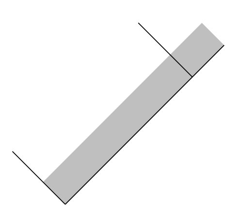
Figure 4: Extension of the initial data on $\mathcal{N}_{\star}$. By causality the choice of the extension of the data beyond $\mathscr{I}^{+}$ does not influence the solution of the causal domain $\mathcal{D}$.

As the workings of the last slice argument have been discussed in detail in Paper I —see section LABEL:PaperI-Section:LastSlice of this reference— here we focus on the necessary modifications. As the main purpose of the present analysis is to ensure that one recovers a portion of future null infinity, in order to ensure existence of the solution to the CEFE on the domain $\mathcal{D}$ one actually needs to show existence in a slightly larger domain. This is because the existence domains are given in terms of open sets. As the CEFE are regular at the sets where $\Xi=0$, one can consider an initial hypersurface $\mathcal{N}_{\star}$ which extends beyond $\mathscr{I}^{+}$. The basic initial data on $\mathcal{N}_{\star}$ as described in Proposition 3 can be extended in an arbitrary but controlled manner beyond the intersection of null infinity with $\mathscr{I}^{+}$ up to, say $v_{\bullet}+\frac{1}{10}$, in such a way that it coincides with the original data for $v\in[0,v_{\bullet}]$ —see Figure 4. In particular we require that the extension is such that the norms $\Delta_{e_{\star},\Xi_{\star}}$, $\Delta_{\Gamma_{\star}}$, $\Delta_{\Sigma_{\star}}$, $\Delta_{\Phi_{\star}}$ and $\Delta_{\phi_{\star}}$ which have a contribution along $\mathcal{N}_{\star}$ are finite. Using this extended data on $\mathcal{N}_{\star}$ together with the data on $\mathcal{N}^{\prime}_{\star}$ and $\mathcal{S}_{\star}$ one can compute the full initial data set for the conformal evolution equations. The last slice argument as discussed in Papers I and II can then be used to ensure existence on

$$\mathcal{D}^{\prime}\equiv\{0\leq u\leq\varepsilon,\;0\leq v\leq v_{\bullet}+\tfrac{1}{10}\}\supset\mathcal{D}.$$

As a consequence of Lemma 4, one has that the set defined by the condition $v=v_{\bullet}$ is a null hypersurface and, accordingly, our domain of existence contains a portion of $\mathscr{I}^{+}$. Finally, observe that by causality the solution on $\mathcal{D}$ is independent of the choice of extended data on $\{u=0,\,v\in(v_{\bullet},v_{\bullet}+\tfrac{1}{10}\}$ —that is, $\mathscr{I}^{+}$ is the Cauchy horizon of the data on $\{v=0,\;u\in[0,\varepsilon\}\cup\{u=0,\;v\in[0,v_{\bullet}]\}$.

7 Application: stability of the Minkowski spacetime from a Cauchy-characteristic initial value problem

In this section we discuss an application of the local extendibility problem of null infinity to the stability of the Minkowski spacetime in a Cauchy-characteristic setting. This argument relies crucially on Friedrich’s semi-global existence and stability result of the Minkowski spacetime from hyperboloidal data —see [19]; see also [10]. The strategy in the proof is to use the local extendibility result of null infinity proven earlier in this article together with the local existence result for the standard Cauchy problem for the conformal Einstein field equations to obtain a development of the Cauchy-characteristic initial data on which one can pass a hyperboloidal hypersurface. If the Cauchy-characteristic initial data is suitably and sufficiently close to data for the Minkowski spacetime then one will be in a situation in which the semi-global stability of the Minkowski spacetime can be used.

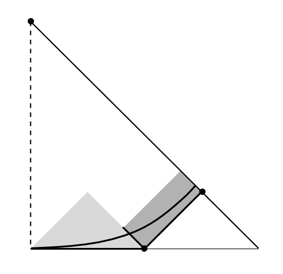
Figure 5: Schematic depiction of the set-up for the proof of the stability of the Minkowski spacetime in a Cauchy-characteristic setting. Cauchy data for the conformal Einstein field equations is provided in the compact spacelike domain $\mathcal{K}_{\star}$ while characteristic data consistent with Lemma 3 is provided on the null hypersurface $\mathcal{N}_{\star}$. This null hypersurface intersects null infinity, $\mathscr{I}^{+}$. The development $D^{+}(\mathcal{K}_{\star})$ (light-grey region) gives rise to characteristic data on the Cauchy horizon $\mathcal{N}^{\prime}_{\star}=H(\mathcal{K}_{\star})$. The theory of the local extendibility of null infinity developed earlier in the article ensures the existence of a solution to the conformal equations in the causal diamond $D(\mathcal{N}_{\star}\cup\mathcal{N}_{\star}^{\prime})$. Crucially, the boundary of this causal diamond includes a portion of $\mathscr{I}^{+}$. On $D^{+}(\mathcal{K}_{\star})\cup D(\mathcal{N}_{\star}\cup\mathcal{N}_{\star}^{\prime})$ one considers a hyperboloidal hypersurface $\mathcal{H}_{\star}$. If the Cauchy-characteristic initial data is assumed to be suitably close to data for the the Minkowski spacetime, then the hyperboloidal data induced on $\mathcal{H}_{\star}$ will also be suitably close to Minkowski hyperboloidal data. Friedrich’s semi-global existence result then ensures that $D(\mathcal{H}_{\star})$ is geodesically complete and has the same global structure as the Minkowski spacetime —in particular, the generators of $\mathscr{I}^{+}$ intersect a point $i^{+}$, spatial infinity.

7.1 Set-up

In the Cauchy-characteristic initial value problem it is assumed one is provided with standard Cauchy initial data for the Einstein field equations in a compact domain $\mathcal{K}_{\star}$ of a spacelike hypersurface $\mathcal{S}_{\star}$. In the following it is assumed that $\mathcal{K}_{\star}=\mathcal{B}_{r_{\star}}$ with $\mathcal{B}_{r_{\star}}$ a solid $3$-dimensional ball of radius $r_{\star}$ as measured by the metric ${\bm{h}}$ of $\mathcal{S}_{\star}$ —in particular, $\partial\mathcal{B}_{r_{\star}}\approx\mathbb{S}^{2}$. Moreover, it is assumed that the hypersurface $\mathcal{S}_{\star}$ is intersected at $\partial\mathcal{B}_{r_{\star}}$ by a null hypersurface $\mathcal{N}_{\star}$ intersecting future null infinity on a cut $\mathcal{C}_{\star}\approx\mathbb{S}^{2}$. A sketch of the the set-up is given in Figure 5.

The initial data on $\mathcal{K}_{\star}$ is assumed to satisfy the Einstein constraint equations. These imply, in turn, a solution to the constraints implied by the conformal Einstein field equations on $\mathcal{K}_{\star}$. In the following, it is assumed that the initial data for the conformal Einstein equations on $\mathcal{K}_{\star}$, to be denoted by $\mathbf{u}_{\star}$, differs from standard (time symmetric) Cauchy data for the Minkowski spacetime, to be denoted by $\mathring{\mathbf{u}}_{\star}$ by at most $\delta>0$ in the standard Sobolev norm of order $s\geq 4$ with $s$ sufficiently large. That is,

$$\parallel\mathbf{u}_{\star}-\mathring{\mathbf{u}}_{\star}\parallel_{s,\mathcal{K}_{\star}}\leq\delta$$

It follows from the theory of symmetric hyperbolic systems that the development of this data will be of class $C^{s-2}$ over its future domain of dependence $D^{+}(\mathcal{K}_{\star})$ —see e.g. [9, 7]. In particular if the initial data has finite $\parallel\;\;\parallel_{s,\mathcal{K}_{\star}}$-norm for every $s\geq 4$, then the solution is of class $C^{\infty}$ over $D^{+}(\mathcal{K}_{\star})$ —this will be assumed in the following for simplicity of presentation. On $\partial\mathcal{B}_{r_{\star}}$ it is assumed that $\mathbf{u}_{\star}$ matches smoothly with characteristic data initial data on $\mathcal{N}_{\star}$ —in the following this data will be denoted by $\mathbf{v}_{\star}$. Similarly, one also considers characteristic data $\mathring{\mathbf{v}}_{\star}$ for the Minkowski spacetime satisfying the assumptions and gauge conditions of Lemma 3 —an explicit construction of this data of the Minkowski spacetime is given in Appendix A.

Now, the improved existence result for the characteristic problem contained in Theorem 2 does not directly provide a statement of Cauchy stability which could be used in the analysis of the non-linear stability of the Minkowski spacetime. The reason for this is the presence of the “number $1$” in the definitions of the quantities $\Delta_{e_{\star},\Xi_{\star}}$, $\Delta_{\Gamma_{\star}}$, $\Delta_{\Phi_{\star}}$ and $\Delta_{\phi_{\star}}$ introduced in Subsection 6.1. This “$1$” was originally introduced in the definition of the analogue quantities quantities in [1] as a safety valve to ensure that the arguments run through even in the case of trivial data. This feature has the consequence that the quantities $\Delta_{e_{\star},\Xi_{\star}}$, $\Delta_{\Gamma_{\star}}$, $\Delta_{\Phi_{\star}}$ and $\Delta_{\phi_{\star}}$ are, strictly speaking, not norms. As it will be shown below, the number “$1$” can be removed from the definition if one has more information about the type of solution one wants to construct —as, for example, closeness to the Minkowski spacetime.

7.2 Cauchy stability for the characteristic initial value problem

In this section it is discussed how to show that if the solution to the CIVP on the causal diamond of Theorem 2 arises from characteristic data $\mathring{\mathbf{v}}_{\star}$ for the Minkowski spacetime, then the solution on the existence diamond is also suitably close to Minkowski data. The precise notion of closeness follows naturally from the strategy of the proof followed in this article for our main theorem.

Start by recalling that as a consequence of Theorem 2 we have already proved the existence of solutions to the CEFE for given arbitrary data on $\mathcal{N}_{\star}$ and $\mathcal{N}^{\prime}_{\star}$. As in the previous subsection assume that on the existence diamond one has two solutions $\mathbf{v}$ and  $\mathring{\mathbf{v}}$ —the later corresponding to the Minkowski spacetime as give, say, in Appendix A. In the following we use the quantities $\xi_{{\bm{e}}}$, $\xi_{\Xi}$, $\xi_{\Gamma}$, $\xi_{\Sigma}$, $\xi_{\phi}$ and $\xi_{\Phi}$ encode the difference of quantities field unknowns between the perturbed and the Minkowski spacetime. For example $\xi_{\mu}\equiv\mu-\mathring{\mu}$ where $\mathring{\mu}$ gives the value of the NP spin connection coefficient on the Minkowski spacetime. For these difference quantities one can define true norms $\Delta_{\xi_{{\bm{e}}_{\star},\Xi_{\star}}}$, $\Delta_{\xi_{\Gamma_{\star}}}$, $\Delta_{\xi_{\Sigma_{\star}}}$, $\Delta_{\xi_{\Phi_{\star}}}$ and $\Delta_{\xi_{\phi_{\star}}}$ and assume such norms are controlled by a small constant $\delta$. These norms are defined in analogous manner to the quantities in Section 6.1 but without the “number $1$” and with the understanding that the derivatives appearing in them are operators on the perturbed spacetime. For example, the norm for the initial value of the differences between connection coefficients is given by

$$\Delta_{\xi_{\Gamma_{\star}}}\equiv\sup_{\mathcal{S}_{u,v}\subset\mathcal{N}_{\star},\mathcal{N}^{\prime}_{\star}}\sup_{\Gamma\in\{\mu,\lambda,\rho,\sigma,\alpha,\beta,\tau,\epsilon\}}\max\{\sum_{i=0}^{1}||/\kern-5.80002pt\nabla^{i}\xi_{\Gamma}||_{L^{\infty}(\mathcal{S}_{u,v})},\sum_{i=0}^{2}||/\kern-5.80002pt\nabla^{i}\xi_{\Gamma}||_{L^{4}(\mathcal{S}_{u,v})},\sum_{i=0}^{3}||/\kern-5.80002pt\nabla^{i}\xi_{\Gamma}||_{L^{2}(\mathcal{S}_{u,v})}\}.$$

Similarly, the norm for the initial value of the difference of the components of the Ricci curvature given is given by

$$\Delta_{\xi_{\Phi_{\star}}}\equiv\sup_{\mathcal{S}_{u,v}\subset\mathcal{N}_{\star},\mathcal{N}^{\prime}_{\star}}\sup_{\Phi\in\{\Phi_{00},\Phi_{01},\Phi_{02},\Phi_{11},\Phi_{12}\}}\max\{\sum_{i=0}^{1}||/\kern-5.80002pt\nabla^{i}\xi_{\Phi}||_{L^{4}(\mathcal{S}_{u,v})},\sum_{i=0}^{2}||/\kern-5.80002pt\nabla^{i}\xi_{\Phi}||_{L^{2}(\mathcal{S}_{u,v})}\}$$

$$+\sum_{i=0}^{3}\sup_{\Phi\in\{\Phi_{00},\Phi_{01},\Phi_{02},\Phi_{11},\Phi_{12}\}}||/\kern-5.80002pt\nabla^{i}\xi_{\Phi}||_{L^{2}(\mathcal{N}_{\star})}+\sup_{\Phi\in\{\Phi_{01},\Phi_{02},\Phi_{11},\Phi_{12},\Phi_{22}\}}||/\kern-5.80002pt\nabla^{i}\xi_{\Phi}||_{L^{2}(\mathcal{N}^{\prime}_{\star})}.$$

Equations for the difference fields can be readily computed by subtraction of the relevant evolution equations. The structure of the resulting equations resembles those of the CEFE with additional terms corresponding to the products between the background (i.e. Minkowski) and difference terms. For example, from the structure equation

$$\Delta\lambda=-2\mu\lambda-\Xi\phi_{4},$$

one obtains that

$$\Delta\xi_{\lambda}\equiv\Delta(\lambda-\mathring{\lambda})=-2\xi_{\mu}\xi_{\lambda}-\xi_{\Xi}\xi_{\phi_{4}}-2\mathring{\mu}\xi_{\lambda}-2\mathring{\lambda}\xi_{\mu}-\mathring{\Xi}\xi_{\phi_{4}}-\mathring{\phi}_{4}\xi_{\Xi}-\frac{\mathring{\Delta}\mathring{\lambda}}{\mathring{Q}}\xi_{Q},$$

where $\mathring{\phi}_{4}$ denotes the component of rescaled Weyl spinors on the Minkowski spacetime (zero!) and $\mathring{\Delta}$ is the derivative along ${\bm{n}}$ on Minkowski. More generally, writing the structure equations in schematic form as

$$D\Gamma-\delta\Gamma=\Gamma\Gamma+\Xi\phi+\Phi,$$

$$\Delta\Gamma-\delta\Gamma=\Gamma\Gamma+\Xi\phi+\Phi,$$

it follows that the associated difference equations are of the form

$$D\xi_{\Gamma}-\delta\xi_{\Gamma}= \xi_{\Gamma}\xi_{\Gamma}+\xi_{\Xi}\xi_{\phi}+\xi_{\Phi}$$

$$+\mathring{\Gamma}\xi_{\Gamma}+\mathring{\Xi}\xi_{\phi}+\mathring{\phi}\xi_{\Xi}+\xi_{P^{\mathcal{A}}}\partial_{\mathcal{A}}\mathring{\Gamma}-\xi_{C^{\mathcal{A}}}\partial_{\mathcal{A}}\mathring{\Gamma},$$

$$\Delta\xi_{\Gamma}-\delta\xi_{\Gamma}= \xi_{\Gamma}\xi_{\Gamma}+\xi_{\Xi}\xi_{\phi}+\xi_{\Phi}$$

$$+\mathring{\Gamma}\xi_{\Gamma}+\mathring{\Xi}\xi_{\phi}+\mathring{\phi}\xi_{\Xi}+\xi_{P^{\mathcal{A}}}\partial_{\mathcal{A}}\mathring{\Gamma}-\frac{\mathring{\Delta}\mathring{\lambda}}{\mathring{Q}}\xi_{Q}.$$

Notice that is the background solution corresponds to the Minkowski spacetime then the Weyl curvature terms $\mathring{\phi}$ actually vanish. From the general structure of these equations it follows that it is possible to obtain estimates for the difference quantities associated to the spin connection coefficients making use of an argument analogous to that used for the actual connection coefficients. For $\xi_{\Sigma}$ and most of the differences $\xi_{\Gamma}$ one can make use of their $\Delta$-equations construct the required estimates. It follows that as long as the short range $\varepsilon$ is sufficiently small, their norms can be bounded by 3 times the size of the initial data.

The analysis of the third order derivatives of $\xi_{\tau}$, $\xi_{\chi}$ and $\xi_{\rho}$ $\xi_{\sigma}$ requires the use of the associated $D$-equations and, thus, require integration along the long direction so as to obtain a Grönwall-type inequality of the form

$$||f||_{L^{p}(\mathcal{S}_{u,v})}\leq C(I,\mathcal{O})\left(||f||_{L^{p}(\mathcal{S}_{u,0})}+\int_{0}^{v}||Df||_{L^{p}(\mathcal{S}_{u,v^{\prime}})}\mathrm{d}v^{\prime}\right),$$

where $\mathcal{O}$ denote a constant related to the spin connection coefficient $\rho$ on the perturbed spacetime. The first term on the right hand side corresponds to initial data for the differences $\xi$ and, thus, is bounded, by assumption, by $\delta$. The second term can be estimated using the $D$-equation; each term in this equation can be bounded by a constant related to the value of the field on the Minkowski spacetime times $\delta$. It follows then that the norm of these particular difference quantities in the solution rectangle can be bounded by $C\delta$ where $C$ is a constant related to the data for the background and perturbed spacetimes. The evolution equations for the difference fields in the short direction can be analysed in analogous manner to what is done for the main Theorem 2 —in this case the argument requires a bootstrap assumption.

Finally, an analogous strategy can be adopted, mutatis mutandi, for the differences fields associated to the components of the Ricci and rescaled Weyl curvature tensors. It is found that in the existence diamond these difference fields are bounded by $C\delta$. Proceeding in this way it is possible to show that in the existence diamond the norms $\Delta_{\xi_{{\bm{e}},\Xi}}$, $\Delta_{\xi_{\Gamma}}$, $\Delta_{\xi_{\Sigma}}$, $\Delta_{\xi_{\Phi}}$ and $\Delta_{\xi_{\phi}}$ can be controlled by $C\delta$ where $C$ denotes again a constant related to the initial data. This observation is a statement of Cauchy stability for the development of characteristic initial data which is close to data for the Minkowski spacetime.

7.3 Statement of the stability result

Following the discussion from the previous subsection, it is assumed that the characteristic initial data $\mathbf{v}_{\star}$ differs from the Minkowski characteristic initial data $\mathring{\mathbf{v}}_{\star}$ in the norms $\Delta_{\xi_{{\bm{e}}_{\star},\Xi_{\star}}}$, $\Delta_{\xi_{\Gamma_{\star}}}$, $\Delta_{\xi_{\Sigma_{\star}}}$, $\Delta_{\xi_{\Phi_{\star}}}$ and $\Delta_{\xi_{\phi_{\star}}}$ by at most $\delta>0$. At the intersection of the initial Cauchy and characteristic hypersurfaces, $\mathcal{K}_{\star}\cap\mathcal{N}_{\star}=\partial\mathcal{B}_{r_{\star}}$, it is assumed that the Cauchy data for the conformal Einstein field equations and the characteristic data on $\mathcal{N}_{\star}$ match smoothly.

Given the above setting, one has the following stability result:

Theorem 3.

Let $\mathcal{K}_{\star}$ and $\mathcal{N}_{\star}$ as in Subsection 7.1. Given smooth initial data for the Einstein field equations on $\mathcal{K}_{\star}$ matching smoothly on $\partial\mathcal{K}_{\star}$ to smooth characteristic data on $\mathcal{N}_{\star}$ extending smoothly to null infinity. If the data on $\mathcal{K}_{\star}\cup\mathcal{N}_{\star}$ is suitably close to Cauchy-characteristic initial data for the Minkowski solution (in the natural norms for $\mathcal{K}_{\star}$ and $\mathcal{N}_{\star}$, respectively) then the future development $D^{+}(\mathcal{K}_{\star}\cup\mathcal{N}_{\star})$ is geodesically complete and has the same global structure than the Minkowski spacetime. In particular, it has a smooth conformal extension with a conformal boundary $\mathscr{I}^{+}$ with complete null generators intersecting at a point $i^{+}$ representing future timelike infinity.

Remark 3.

For simplicity of presentation, the above theorem has been stated in the smooth (i.e. $C^{\infty}$) class. However, a detailed analysis of the proof, and, in particular, of the argument leading to the result on the local extension of future null infinity, Theorem 2 should lead to sharp statements in terms of the assumed regularity of the initial conditions and the resulting regularity of the solution. This analysis, is not be pursued presently.

7.4 Proof

Given the set-up described in the previous paragraphs, the argument to show the stability of the Minkowski spacetime from Cauchy-characteristic data proceeds as follows:

• The Cauchy data given on $\mathcal{K}_{\star}$ gives rise to a future development $D^{+}(\mathcal{K}_{\star})$. As this data does not cover the whole of a Cauchy hypersurface, the development has a Cauchy horizon $H^{+}(\mathcal{K}_{\star})$. The general theory of Lorentzian theory ensures that $H^{+}(\mathcal{K}_{\star})$ is a smooth null hypersurface [20]. Moreover, choosing the existence time of the development of $\mathcal{K}_{\star}$ sufficiently small one ensure that the solution to the conformal Einstein field equations on $D^{+}(\mathcal{K}_{\star})$ extends smoothly to $H^{+}(\mathcal{K}_{\star})$. Now, setting $\mathcal{N}_{\star}^{\prime}=H^{+}(\mathcal{K}_{\star})$ the restriction of the solution to the conformal Einstein field equations implies characteristic data on $\mathcal{N}^{\prime}_{\star}$ in the sense of Lemma 3 which is suitably close to characteristic data for the Minkowski spacetimes. Observe that for exact Minkowski data one has $\phi_{4}=0$ on $\mathcal{N}^{\prime}_{\star}$.

• The full characteristic data on $\mathcal{N}_{\star}\cup\mathcal{N}^{\prime}_{\star}$ give rise to development $D^{+}(\mathcal{N}^{\prime}_{\star}\cup\mathcal{N}_{\star})$ in the form of a causal diamond which, by the theory developed in the previous sections of this article has one side coinciding with a portion of future null infinity $\mathscr{I}^{+}$. A detailed inspection of the last slice argument shows, in particular, that if the data on the initial characteristic hypersurface $\mathcal{N}_{\star}\cup\mathcal{N}^{\prime}_{\star}$ is smooth, then the development $D^{+}(\mathcal{N}^{\prime}_{\star}\cup\mathcal{N}_{\star})$ is also smooth.

• Now, the Cauchy-characteristic development $D^{+}(\mathcal{K}_{\star})\cup D^{+}(\mathcal{N}^{\prime}_{\star}\cup\mathcal{N}_{\star})$ contains a smooth hyperboloid $\mathcal{H}_{\star}$. An explicit example can be given as follows: consider the (physical) Minkowski spacetime $(\mathbb{R}^{4},\tilde{{\bm{\eta}}})$ in spherical coordinates $(\tilde{t},\tilde{r},x^{\mathcal{A}})$. Then the upper sheet of the hypersurface given by the condition

  $$\frac{(\tilde{t}+a)^{2}}{a^{2}}-\frac{\tilde{r}^{2}}{1-a^{2}}=1$$ (6)

  with $a=\tfrac{1}{2}\sqrt{5}-\tfrac{1}{2}$ is an hyperboloidal hypersurface passing through the origin. In particular, for large $r$ the hyperboloid asymptotes the null hypersurface described by the condition

  $$\tilde{t}-\tilde{r}=0.$$

  The conformal factor

  $$\Theta=\cos t+\cos r$$

  where

  $$\tilde{t}=\frac{\sin t}{\cos t+\cos r},\qquad\tilde{r}=\frac{\sin r}{\cos t+\cos r},$$

  with $t\in[-\pi,\pi]$, $r\in[0,\pi]$ gives an embedding of the Minkowski spacetime into the Einstein cylinder. Now, as we are working with a perturbation of the Minkowski spacetime, the coordinates $(t,r,x^{\mathcal{A}})$ can also be used, in a slight abuse of notation, as coordinates of the perturbed spacetime. The upper sheet of the hypersurface described by the condition (6) expressed in terms of the coordinates $(t,r)$ given above is also an hyperboloid on $D^{+}(\mathcal{K}_{\star})\cup D^{+}(\mathcal{N}^{\prime}_{\star}\cup\mathcal{N}_{\star})$.

• As the initial data on $\mathcal{K}_{\star}\cup\mathcal{N}_{\star}$ is assumed to be suitably close to Cauchy-characteristic initial data for the Minkowski spacetime, then the solution to the conformal Einstein field equations on $D^{+}(\mathcal{K}_{\star})\cup D^{+}(\mathcal{N}_{\star})$ is also suitably close to the Minkowski solution. By construction, in the compound domain $D^{+}(\mathcal{K}_{\star})\cup D^{+}(\mathcal{N}^{\prime}_{\star}\cup\mathcal{N}_{\star})$, the resulting solution to the conformal Einstein field equations is smooth and controlled by the Cauchy-characteristic initial data on $\mathcal{K}_{\star}\cup\mathcal{N}_{\star}$. In particular, due to the smoothness of the solution, one gets control at the level of the supremum norm over the whole of any derivatives $D^{+}(\mathcal{K}_{\star})\cup D^{+}(\mathcal{N}^{\prime}_{\star}\cup\mathcal{N}_{\star})$. Observe that as the domain is compact then the supremum of any of the conformal fields coincides with the maximum.

• As the solution on $D^{+}(\mathcal{K}_{\star})\cup D^{+}(\mathcal{N}^{\prime}_{\star}\cup\mathcal{N}_{\star})$ is smooth, it follows that, $\mathbf{w}_{\star}$, the implied hyperboloidal initial data for the conformal Einstein field equations on $\mathcal{H}_{\star}$ is smooth. Moreover, as in the conformal picture the hyperboloid $\mathcal{H}_{\star}$ is a compact 3-manifold, it follows then that all the derivatives of the induced hyperboloidal data are in $L^{2}(\mathcal{H}_{\star})$ so that $\mathbf{w}_{\star}\in H^{s}(\mathcal{H}_{\star})$ for all $s\geq 4$. By choosing $\varepsilon>0$ in the Cauchy-characteristic initial data sufficiently small, one can make sure that $\mathbf{w}_{\star}$ is suitably close to hyperboloidal data for the Minkowski solution.

• Applying Friedrich’s semi-global stability result for the Minkowski spacetime to the hyperboloidal data $\mathbf{w}_{\star}$ on $\mathcal{H}_{\star}$ it follows that one obtains a smooth future development $D^{+}(\mathcal{H}_{\star})$ with Cauchy horizon $H^{+}(\mathcal{H}_{\star})$ which an be identified with future null infinity $\mathscr{I}^{+}$. The null hypersurface $\mathscr{I}^{+}$ has generators which are future complete and which intersect at a point $i^{+}$ —timelike infinity.

• The solution to the conformal Einstein field equations on $D^{+}(\mathcal{K}_{\star})$ implies, whenever $\Xi\neq 0$ a solution to the Einstein field equation which is future geodesically complete and with the same global asymptotic structure than the Minkowski spacetime.

Appendix A A conformal representation of Minkowski in Stewart’s gauge

In this appendix we discuss a conformal representation of the Minkowski spacetime in Stewart’s gauge.

In the following, let $(\tilde{\mathcal{M}},\tilde{{\bm{\eta}}})$ denote the Minkowski spacetime and let $\bar{x}=(x^{\mu})$ correspond to standard Cartesian coordinates so that

$$\tilde{{\bm{\eta}}}=\eta_{\mu\nu}\mathbf{d}x^{\mu}\otimes\mathbf{d}x^{\nu}$$

$$\phantom{\tilde{{\bm{\eta}}}}=\mathbf{d}x^{0}\otimes\mathbf{d}x^{0}-\mathbf{d}x^{1}\otimes\mathbf{d}x^{1}-\mathbf{d}x^{2}\otimes\mathbf{d}x^{2}-\mathbf{d}x^{3}\otimes\mathbf{d}x^{3}.$$

Consider now the domain

$$\tilde{\mathcal{D}}\equiv\{p\in\mathbb{R}^{4}\;|\;\eta_{\mu\nu}x^{\mu}(p)x^{\nu}{p}<0\},$$

corresponding to the complement of the light cone through the origin. A suitable conformal representation of this domain is obtained via the coordinate inversion defined by

$$y^{\mu}=-\frac{x^{\mu}}{X^{2}},\qquad X^{2}\equiv\eta_{\mu\nu}x^{\mu}x^{\nu},$$

so that

$$\eta_{\mu\nu}\mathbf{d}y^{\mu}\otimes\mathbf{d}y^{\nu}=X^{-4}\eta_{\mu\nu}\mathbf{d}x^{\mu}\otimes\mathbf{d}x^{\nu}.$$

Accordingly defining the conformal factor $\Xi\equiv X^{-2}$ one obtains the conformal metric ${\bm{\eta}}=\Xi^{2}\tilde{{\bm{\eta}}}$. Observe that

$${\bm{\eta}}=\eta_{\mu\nu}\mathbf{d}y^{\mu}\otimes\mathbf{d}y^{\nu},$$

so that this conformal representation of $\tilde{\mathcal{D}}$ is flat —in particular, the Ricci scalar of ${\bm{\eta}}$ vanishes. Of particular relevance for the subsequent analysis is that future null infinity is described by

$$\mathscr{I}^{+}=\{p\in\mathbb{R}^{4}\;|\;y^{0}(p)>0,\;\eta_{\mu\nu}y^{\mu}(p)y^{\nu}(p)=0\}.$$

In order to set up Stewart’s gauge consider, first, standard spherical coordinates $(t,t,\theta,\varphi)$ and then, in turn, double null coordinates $(u,v,\theta,\phi)$ such that

$$u=\frac{1}{\sqrt{2}}(t-r),\qquad v=\frac{1}{\sqrt{2}}(t+r),$$

for which one has

$${\bm{\eta}}=\mathbf{d}u\otimes\mathbf{d}v+\mathbf{d}v\otimes\mathbf{d}u-(u-v)^{2}{\bm{\sigma}}.$$ (7)

In particular, $\mathscr{I}^{+}$ is given by the condition $v=0$. Redefining $v$ through an translation one can set the location of $\mathscr{I}^{+}$ to be given by the condition $v=v_{\bullet}$, for some $v_{\bullet}>0$. A NP frame satisfying the conditions of Stewart’s gauge can be obtained by setting

$${\bm{l}}={\bm{\partial}}_{v},\qquad{\bm{n}}={\bm{\partial}}_{u},\qquad{\bm{m}}=\frac{(u-v)}{\sqrt{2}}({\bm{\partial}}_{\theta}+\mbox{i}\csc\theta{\bm{\partial}}_{\bm{\varphi}}),$$

so that

$$Q=1,\qquad C^{\mathcal{A}}=0,\qquad P^{2}=\frac{u-v}{\sqrt{2}},\qquad P^{3}=\frac{\mbox{i}(u-v)}{\sqrt{2}}\csc\theta.$$

A computation readily shows that the NP spin connection coefficients associated to the above tetrad are

$$\kappa=\tau=\sigma=\pi=\nu=\lambda=\epsilon=\gamma=0,$$

$$\rho=\mu=\displaystyle\frac{1}{u-v},\quad\alpha=-\beta=\displaystyle\frac{\cot\theta}{2\sqrt{2}(u-v)}.$$

The above coefficients can be readily seen to satisfy the conditions of Stewart’s gauge. Moreover, as the metric (7) is flat one has that

$$\phi_{0}=\phi_{1}=\phi_{2}=\phi_{3}=\phi_{4}=0,$$

$$\Phi_{00}=\Phi_{01}=\Phi_{02}=\Phi_{10}=\Phi_{11}=\Phi_{12}=\Phi_{20}=\Phi_{21}=\Phi_{22}=0,$$

$$\Lambda=0.$$

The above expressions imply regular characteristic data as given by Lemma 3.

References

- [1] J. Luk. On the local existence for the characteristic initial value problem in general relativity. Int. Math. Res. Not., 20:4625, 2012.
- [2] A. D. Rendall. Reduction of the characteristic initial value problem to the cauchy problem and its application to the einstein equations. Proc. Roy. Soc. Lond. A, 427:221, 1990.
- [3] D. Hilditch, J. A. Valiente Kroon, and P. Zhao. Revisiting the characteristic initial value problem for the vacuum einstein field equations. in arXiv 1911.00047, 2019.
- [4] J. Stewart. Advanced general relativity. Cambridge University Press, 1991.
- [5] D. Hilditch, J. A. Valiente Kroon, and P. Zhao. Improved existence for the characteristic initial value problem with the conformal einstein field equations. In arXiv:2006.13757[gr-qc], 2020.
- [6] J. Li and X.-P. Zhu. On the local extension of the future null infinity. J. Diff. Geom., 110:73, 2018.
- [7] J. A. Valiente Kroon. Conformal Methods in General Relativity. Cambridge University Press, 2016.
- [8] H. Friedrich. Some (con-)formal properties of Einstein’s field equations and consequences. In F. J. Flaherty, editor, Asymptotic behaviour of mass and spacetime geometry. Lecture notes in physics 202. Springer Verlag, 1984.
- [9] H. Friedrich. On the existence of n-geodesically complete or future complete solutions of Einstein’s field equations with smooth asymptotic structure. Comm. Math. Phys., 107:587, 1986.
- [10] C. Lübbe and J. A. Valiente Kroon. On de sitter-like and minkowski-like spacetimes. Class. Quantum Grav., 26:145012, 2009.
- [11] L. Andersson, P. T. Chruściel, and H. Friedrich. On the regularity of solutions to the Yamabe equation and the existence of smooth hyperboloidal initial data for Einstein’s field equations. Comm. Math. Phys., 149:587, 1992.
- [12] L. Andersson and P. T. Chruściel. Hyperboloidal cauchy data for vacuum einstein equations and obstructions to smoothness of null infinity. Phys. Rev. Lett., 70:2829, 1993.
- [13] L. Andersson and P. T. Chruściel. On “hyperboloidal” Cauchy data for vacuum Einstein equations and obstructions to smoothness of scri. Comm. Math. Phys., 161:533, 1994.
- [14] P. Szekeres. The gravitational compass. J. Math. Phys., 6:1387, 1965.
- [15] R. Penrose and W. Rindler. Spinors and space-time. Volume 2. Spinor and twistor methods in space-time geometry. Cambridge University Press, 1986.
- [16] O. Graf. Global nonlinear stability of minkowski space for spacelike-characteristic initial data. In arXiv:2010.12434 [math.AP], 2020.
- [17] R. Penrose and W. Rindler. Spinors and space-time. Volume 1. Two-spinor calculus and relativistic fields. Cambridge University Press, 1984.
- [18] J. M. Stewart and H. Friedrich. Numerical relativity. The characteristic initial value problem. Proc. Roy. Soc. Lond. A, 384:427, 1982.
- [19] H. Friedrich. On purely radiative space-times. Comm. Math. Phys., 103:35, 1986.
- [20] S. W. Hawking and G. F. R. Ellis. The large scale structure of space-time. Cambridge University Press, 1973.