Optimal control policies for resource allocation in the Cloud: comparison between Markov decision process and heuristic approaches

Abstract

We consider an auto-scaling technique in a cloud system where virtual machines hosted on a physical node are turned on and off depending on the queue’s occupation (or thresholds), in order to minimise a global cost integrating both energy consumption and performance. We propose several efficient optimisation methods to find threshold values minimising this global cost: local search heuristics coupled with aggregation of Markov chain and with queues approximation techniques to reduce the execution time and improve the accuracy. The second approach tackles the problem with a Markov Decision Process (MDP) for which we proceed to a theoretical study and provide theoretical comparison with the first approach. We also develop structured MDP algorithms integrating hysteresis properties. We show that MDP algorithms (value iteration, policy iteration) and especially structured MDP algorithms outperform the devised heuristics, in terms of time execution and accuracy. Finally, we propose a cost model for a real scenario of a cloud system to apply our optimisation algorithms and show their relevance.
Keywords :
Decision processes, Markov Processes, Hysteresis Queues, Heuristics, Cloud System, Reducing Energy, Quality of Service

1 Introduction

Rapid growth of the demand for computational power by scientific, business and web-applications has led to the creation of large-scale data centers which are often oversized to ensure the quality of service of hosted applications. This leads to an under-utilisation of the servers which implies important electric losses and over-consumption. Nowadays, Cloud computing requires more electric power than those of whole countries such as India or Germany [1, 2]. To improve the utilisation rate of servers, some data center owners have deployed some methods implementing dynamicity of resources according to system load. Those mechanisms, called “autoscaling” [3] are based on activation and deactivation of Virtual Machines (VMs) [4] according to the workload.

Nevertheless, it is crucial to analyse both the energy consumption and the performance of the system to find the policy that adapts resource allocation to the demand. Unfortunately, these two measures are inversely proportional, which motivates researchers to evaluate them simultaneously via a unique global cost function. In order to adapt resources, some queueing systems modulate the service capacity according to queue occupancy, these are hysteresis models [5]. They allow not to activate and deactivate the servers too frequently when the load is varying. This makes it possible to correctly adapt variable resources according to demand by means of thresholds [6, 7]. Therefore, multi-server queueing systems working with thresholds-based policies and verifying hysteresis properties have been suggested to efficiently manage the number of active VMs [8, 5, 9]. The other advantage that makes hysteresis policies so appealing is their ease of implementation. This is why, they are a key component of the auto-scaling systems for the widespread cloud architectures Kubernetes for docker components, and Azure or Amazon Web Services [10] for virtual machines. Henceforth, there is a great interest of studying the computation of hysteresis policy since threshold values can be plugged into autoscaling systems that are implemented in the major cloud architectures.

In this work, we consider a cost-aware approach. We propose a model with a global expected cost considering different costs: associated with the performance requirements defined in a Service Level Agreement (SLA) and associated with energy consumption. Two modelling approaches are addressed: static optimisation problem or dynamic control. The static optimisation problem expresses the problem by using the average value of the costs computed by stationary distribution of a CTMC (Continuous Time Markov Chains). Such an approach is often used in the field of inventory management for base stock policies [11]. On the other hand, dynamic control expresses the problem under a MDP (Markov Decision Process) model and computes the optimal policy.

We propose new scalable and efficient algorithms for minimisation of the global cost. For static optimisation the work [9] presents and compares several heuristics but is restricted to the static model. In the present paper, we first improve the previous heuristics of [9] by modifying several stages and present new algorithms for the static model. We design completely new algorithms based on optimal dynamic control integrating hysteresis policies and we show that they are much faster while ensuring the optimality of the solution. Although they are the most widely used for threshold computation [12], the efficiency of these two approaches are not assessed very well in the literature for the computation of single thresholds by level. Especially, this had been never done for hysteresis policies. Determining which is the best promising approach is thus a major point which is addressed here by performing numerous numerical experiments. Furthermore, numerical results show that we can generate the thresholds corresponding to the optimized global cost in just few seconds even for large systems. This could have a significant impact for a cloud operator who wants to dynamically allocate its resources to control its financial costs.

The key contributions of this paper are as follows:

1. We improve the existing heuristics of [9] that makes a large review of the heuristics of the literature which solve static optimisation problems. We assess numerically the gain given by these improvements;

2. We provide a theoretical study of the multichain properties of the Markov decision process. This shows that some usual algorithms solving MDP models have no convergence guarantee. We still provide an algorithm that solves dynamic control model by considering hysteresis assumption in the MDP;

3. We made a theoretical analysis between the two approaches and give some insights which explain why the static optimisation problem is suboptimal. Numerical studies show that the dynamic control approach strongly outperforms the other one for optimality and running time criteria;

4. We develop and analyse a financial cost model. It takes into account prices of VM instantiations from cloud providers as well as energy consumption of VMs. A presentation of minimised costs for a problem based on this concrete cloud model is done.

The remainder of this paper is organised as follows. Section 2 briefly reviews the related works. In Section 3, we provide a treatment to unify the different definitions of hysteresis policies coming from different models. Then, we describe the cloud system, with the queueing model. We detail the cost function used to express the expected costs in terms of performance and energy consumption for such models. In Section 4, we present the Markov chain approach with the decomposition and aggregation method, and the optimisation algorithms based on local search heuristics. We also present a Markov decision process model and adapted algorithms in Section 5. Section 6 presents a concrete cost model. Numerical experiments for the comparison of the algorithms are discussed in Section 7. In the conclusion, we finally discuss about achieved results. Some comments about further researches are given.

2 Literature review

2.1 Energy and Performance Management in the Cloud

In recent years, the increase in the energy consumption has remained a crucial problem for large-scale computing. In a data center, the server power consumption can be divided into static and dynamic parts. The static part (which does not vary with workload) represents the energy consumed by a server when it is idle, while the dynamic cost depends on the current usage. In [13], they define a power-aware model to estimate the dynamic part of energy cost for a VM of a given size, this model keeps the philosophy of the pay as you go model but it is based on energy consumption.

As the static part represents a high part of the overall energy consumed by the server nodes, therefore, shutting unused physical resources that are idle lead to non-negligible energy savings. Two main approaches of physical server resource management have been proposed to improve the energy efficiency: shutdown or switching on servers or VMs which is referred as dynamic power management [4], and scaling of the CPU performance which is referred as Dynamic Voltage and Frequency Scaling [14]. Shutdown strategies (considered here) are often combined with consolidation algorithms that gather the load on few servers to favour the shutdown of the others. So, managing energy by switching on or switching off virtual machines is an intuitive and widespread manner to save energy. Yet, as quoted in [4], coarse techniques of shutdown are, most often, not the appropriate solution to achieve energy reduction. Indeed, shutdown policies suffer from energy and time losses when switching off and switching on take longer than the idle period.

2.2 Control Management for Queueing Models

In order to represent the problems with activations and deactivations of virtual machines, server farm models have been proposed [15, 16, 17]. Usually, these server farm models are modeled with multi-server queueing systems [18, 19]. Although server farms with multi-server queues allow a fairly fine representation of the dynamicity induced by virtualization, these models do not address issues related neither to the internal network nor to the VM placement in it. All VMs are instead considered as parallel resources. This makes these models suitable for studying simple nodes of several servers in the cloud. If queuing models allow us to easily compute performance metrics, the decision making for switching on or switching off the VM requires an additional step which remains a key point. The computation of the optimal actions has led to a large field of researches and methods. Dynamic control and especially Markov decision Processes appear to be the main direct method.

2.3 Markov Decision Process and Hysteresis Policies

Since the seminal work of Mc Gill in 1969 (with an optimal control model) and that of Lippman (with a Markov decision process model) numerous works have been devoted to similar multi-server queue models using Markov decision processes (see [20] and references therein for the oldest, and more recently [21] and [22] to quote just a few). Unfortunately, not all of them received rigorous treatment and the study of unichain or multichain property is often ignored. It appeared very early, in the work of Bell for a $M/M/2$ model (see [20]), that the optimal policy in such models has a special form and is called hysteresis. In hysteresis policies, servers are powered up when the number of jobs in the system is sufficiently high and are powered down when that number is sufficiently low. More precisely, activations and deactivations of servers are ruled by sequences of different forward and reverse thresholds. The concept of hysteresis can also be applied to the control of service rates.

Researches on hysteresis policies are twofold: first exploration of the conditions that insure the optimality of hysteresis policy. Hence, Szarkowicz et al. [23] showed the optimality of hysteresis policies in a $M/M/S$ queueing model with a control of the vacations of the servers. For models with control of the service rates, the proofs are made in Hipp [24] or Serfozo [6]. The second axis studies the computation of the threshold values.

2.4 Threshold calculation methods

For hysteresis models, the calculation of optimal thresholds received less attention in the past. Also here two major trends appeared. The computation of the optimal policy can be done by means of adapted usual dynamic programming algorithms in which the structured policies properties are plugged. A similar treatment has been addressed for routing in [25]. The alternate way is similar to the single threshold research for base-stock policies which is very common in inventory management. A local search [26, 27] is used to explore the optimal thresholds. The computation of expected measures associated with a set of thresholds is complex [28]. It requires the computation of the stationary distribution either by standard numerical methods see e.g. [29] or after a Markovian analysis with simpler and faster computations (e.g. [11] uses iterative methods to compute the stationary distribution). In [12], Song claims that, for single threshold models, the second approach dealing with stationary distribution computations are generally more effective than the MDP approach. Such a comparison has not been performed yet for hysteresis especially since few works implement a MDP algorithm with a structured policy.

As cloud systems are modelled by multi-dimensional systems, defined on very large state spaces, then the stationary distribution computation is difficult. Fortunately, the computation of the performance measures of hysteresis multi-server systems has been already studied in the literature. Different efficient resolution methods have been developed. Among the most significant works, we quote the work of Ibe and Keilson [30] refined in Lui and Golubchik [7]. Both solve the model by partitioning the state space in disjoint sets to aggregate the Markov chain. Exhaustive comparisons of the resolution methods are made in [31]: closed-form solution of the stationary distribution, partition of the state space, and matrix geometric methods applied on QBD (Quasi birth and death) processes are studied. It was noticed that partitioning is the most suited. Furthermore, for optimisation, the objective cost function being non-linear and non-convex makes this problem very complex and there is currently no exact method to solve this problem. The work [27] presents three heuristics for searching single thresholds in inventory models that have been adapted for hysteresis in [9]. These approximate heuristics require the computation of the invariant distribution and the cost for numerous threshold values which requires very high computation times. For a server farm model with activation of a single reserve threshold, Mitrani [17] uses fluid approximation to compute the activation thresholds and [29] uses genetic algorithm for optimisation and matrix geometric method for the stationary distribution computation.

3 Cloud Model

In this section, we present the cloud system, denoted Cloud Model, and modelled by a controlled multi-server queueing model, where arrivals of requests are processed by servers. The servers in the queueing system represent logical units in the cloud. Since we consider IaaS clouds (Infrastructure as a Service) which provide computing resources as a service, the logical units are either virtual machines or docker components. We propose a mathematical analysis of the queueing model in order to derive performance as well as energy consumption measures.

3.1 Controlled multi-server queue

We have following assumptions for the model:

1. Arrivals of requests follow a Poisson process of rate $\lambda$, and service times of all VMs are independent of arrivals and independent of each other. Moreover, they are i.i.d. and follow an exponential distribution with an identical rate $\mu$;

2. Requests enter in the queue, which has a finite capacity $B$, and are served by one of the $K$ servers. The service discipline is supposed FIFO (First In First Out).

A customer is treated by a server as soon as this server becomes idle and the server is active. Servers can be turned on and off by the controller. When the server is turned on it becomes active while it becomes inactive when it is turned off.

We define $\mathcal{S}$ the state space, where $\mathcal{S}=\{0,1,\ldots,B\}\times\{1,\ldots,K\}$. Any state $x\in\mathcal{S}$ is such that $x=(m,k)$ where $m$ represents the number of requests in the system, and $k$ is the number of operational servers (or active servers, this number can also be seen as a service level). We define $\mathcal{A}=\{0,\ldots,K\}$, be the set of actions, where action $a$ denotes the number of servers to be activated. With this system, are associated two kinds of costs that a cloud provider encounters:

1. Costs corresponding to the performance of the system, for the control of the service quality defined in the SLA: as costs ($C_{H}$) per unit of time for holding requests in the queue or instantaneous costs ($C_{R}$) for losses of requests.

2. Costs corresponding to the use of resources (operational and energy consumption): as costs for using a VM per unit of time ($C_{S}$) and instantaneous costs for activating/deactivating ($C_{A}$ and $C_{D})$.

We define for the system a global cost containing both performance and energy consumption costs. We have the following objective function we want to minimise:

$$\bar{C}=\lim_{T\rightarrow\infty}\frac{1}{T}\,\mathbb{E}\Biggl{\{}\int_{0}^{T}C_{t}\left(X(t),A(t)\right)dt\Biggr{\}}$$ (1)

where $A(t)$ is the action taken at time $t$ (it is possible that nothing was performed) and $C_{t}(X(t),A(t))$ is the cost that is charged over time when the state is $X(t)$ and action $A(t)$ is performed. This problem can be solved using dynamic programming algorithms or by computing the corresponding thresholds values for turning on and off the VMs.

3.2 Models of hysteresis policies

A decision rule is a mapping from some information set to some action. A policy is a sequence of decision rules $\eta=(q_{0},q_{1},q_{2},\ldots)$. The most general set of policies is that of history-dependent randomised policies, but the classical results on average infinite-horizon, time-homogeneous Markovian optimal control [32] allow us to focus on stationary Markov Deterministic Policies. Such policies are characterised by a single, deterministic decision rule which maps the current state to an action. We thus consider the mapping $q$ from $\mathcal{S}$ to $\mathcal{A}$ such that $q(x)=a$.

All along the paper we restrict our attention with a special form of policies: the hysteresis policies. Nevertheless, there is relatively few homogeneities between definitions of hysteresis policies in the literature. Indeed, it can refer to policies defined with double thresholds (especially when $K=2$), or to a restrictive definition when Markov chains are used. We follow the works of [24, 6] to present an unified treatment of hysteresis.

Hysteresis policies with multiple activations

We assume in this part that the decision rule is a mapping from the state to a number of active servers $q(m,k)=k_{1}$ with $k_{1}\in[1,\ldots,K]$. Several servers can be activated or deactivated to pass from $k$ to $k_{1}$ active servers.

Definition 1 (Double threshold policies).

We call double threshold policy a stationary policy such that the decision rule $q(m,k)$ is increasing in both of its arguments and is defined by a sequence of thresholds such that for any $k$ and $k_{1}$ in $[1,K]$ we have:

$$q(m,k)=k_{1}\text{ when }\quad\ell_{k_{1}}(k)\leq m<\ell_{k_{1}+1}(k)\,,$$

where $\ell_{k_{1}}(k)=\min\{m:q(m,k)\geq k_{1}\}$. This minimum is $\infty$ if the set is empty. For all $k$, we also fix $\ell_{K+1}(k)=\infty$ and $\ell_{1}(k)=0$ (since at least one server must be active).

A monotone hysteresis policy is a special case of double threshold policy.

Definition 2 (Monotone Hysteresis polices [24]).

A policy is a monotone hysteresis policy if it is a double threshold policy and moreover if there exist two sequences of integers $l_{k}$ and $L_{k}$ such that

$$l_{k}=\ell_{k}(K)=\ell_{k}(K-1)=\ldots=\ell_{k}(k)$$

$$L_{k}=\ell_{k}(1)=\ell_{k}(2)=\ldots=\ell_{k}(k-1)\,,$$

with $l_{k}\leq L_{k}\ \text{ for }\ k=1,\ldots,K+1$ ; $l_{k}\leq L_{k+1}\ \text{ for }\ k=1,\ldots,K\,$ ; $l_{1}=L_{1}=0$, $l_{K+1}=L_{K+1}=\infty$. And if, for all $(m,k)\in\mathcal{S}$,

$$q(m,k)=\begin{cases}q(m,k-1)&\text{ if }m<l_{k}\text{ and }k>1\\ k&\text{ if }l_{k}\leq m<L_{k+1}\\ q(m,k+1)&\text{ if }m\geq L_{k+1}\text{ and }k<m\end{cases}\,.$$

The thresholds $l_{k}$ can be seen as the queue levels at which some servers should be deactivated and the $L_{k+1}$ are the analogous activation points. Roughly speaking, the difference between a double threshold and a monotone hysteresis policy lies in the fact that some thresholds toward a level are identical in hysteresis.

Definition 3 (Isotone Hysteresis polices [24]).

] A policy is an isotone policy if it is a monotone hysteresis policy and if $0=l_{1}\leq l_{2}\leq\ldots\leq l_{K+1}=\infty\text{ and }0=L_{1}\leq L_{2}\leq\ldots\leq L_{K+1}=\infty$.

Example 1.

In Figure 1, we represent an isotone policy. The number indicates the number of servers that should be activated in each state. The bold line means that the number of activated servers is the same than the decision and then no activation or deactivation have to be performed.

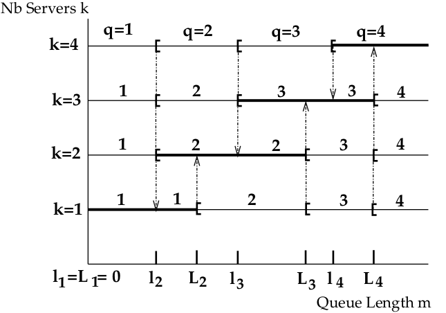
Figure 1: An isotone hysteresis policy.

Proposition 1 (Optimality of monotone hysteresis policies [23]).

In the multi-server queueing model presented in Section 3 and for which there is activation/deactivation costs, working costs and holding costs, Szarkowicz and al. showed that monotone hysteresis policies are optimal policies.

However, the presence of a rejection cost, as we assume here, is not considered in the assumptions of [23] and there is no proof about the optimality of hysteresis policies for the model studied here.

Remark.

There is an alternate way to express the policy by giving the number of servers to activate or deactivate instead of giving directly the number of servers that should be active.

Hysteresis policies with single VM activation

We focus now on models in which we can only operate one machine at a time. Now the decision rule indicates an activation or deactivation. Therefore, the action space is now $\mathcal{A}=\{-1,0,1\}$. For a state $(m,k)$, when the action $q\in\mathcal{A}$ is $-1$ then we deactivate a server, when the action is $0$ then the number of active servers remains identical, when the action is $1$ then we activate a server.

It could be noticed that, for this kind of model, double threshold policies and hysteresis policies coincide. Indeed, the decision now relates to activation (resp. deactivation) and no longer to the number of servers to activate (resp. deactivate). There exist only two thresholds by level $k$: $L_{k+1}$ to go to level $k+1$, and $l_{k}$ to go to level $k-1$. There are no other levels that can be reached from $k$. For example, in Figure 1 all decisions smaller than the level are replaced by $-1$ while all decisions larger than the level are replaced by $1$. Definition 3 remains unchanged, but Definition 2 should be rephrased in:

Definition 4 (Monotone hysteresis policy).

A policy is a monotone hysteresis policy if it is a stationary policy such that the decision rule $q(m,k)$ is increasing in $m$ and decreasing in $k$ and if is defined by two sequences of thresholds $l_{k}$ and $L_{k}$ such that for all $(m,k)\in\mathcal{S}$:

$$q(m,k)=\begin{cases}-1&\text{ if }m<l_{k}\text{ and }k>1\\ \ 0&\text{ if }l_{k}\leq m<L_{k+1}\\ \ 1&\text{ if }m\geq L_{k+1}\text{ and }k<m\end{cases}\,,$$

with $l_{k}\leq L_{k}$ for $k=1,\ldots,K+1$ ; $l_{k}\leq L_{k+1}$ for $k=1,\ldots,K$ and $l_{1}=L_{1}=0\,;l_{K+1}=L_{K+1}=\infty.$

Hysteresis policies and Markov chain

As presented in [20], there exists a slightly different model of multi-server queue with hysteresis policy which received a lot of attention (see Ibe and Keilson [30] or Lui and Golubchik [7] and references therein). This model is still a multi-server queueing system but is no longer a controlled model: the transitions between levels are also governed by sequences of prefixed thresholds this is why it is called an hysteresis model. It is built to be easily represented by a Markov chain. The differences between the controlled model and this Markov chain model are detailed in Section 5.3.

Remark.

For convenience, deactivation and activation thresholds will be denoted respectively by $R$ and $F$ in the Markov chain model, while they will be denoted $l$ and $L$ in the MDP model.

Definition 5 (Hysteresis policy [7]).

A $K$-server threshold-based queueing system with hysteresis is defined by a sequence $F=[F_{1},F_{2},\ldots,F_{K-1}]$ of activation thresholds and a sequence $[R_{1},R_{2},\ldots,R_{K-1}]$ of deactivation thresholds. For $1\leq k<K$, the threshold $F_{k}$ makes the system goes from level $k$ to level $k+1$ when a customer arrives with $k$ active servers and $F_{k}$ customers in the system. Conversely, the threshold $R_{k}$ makes the system goes from level $k+1$ to level $k$ when a customer leaves with $k+1$ active servers and $R_{k}+1$ customers in the system.

Furthermore, we assume that $F_{1}<F_{2}<\ldots<F_{K-1}\leq K$, $1\leq R_{1}<R_{2}<\ldots<R_{K-1}$, and $R_{k}<F_{k}$, $\forall\,1\leq k\leq K-1$. We denote the vector that gathers the two threshold vectors $F$ and $R$ by $[F,R]$.

Remark.

It can be noticed that, no server can remain idle all the time here since the threshold values are bounded, whereas in Definition 4 when a threshold is infinite the server remains inactive. Hence the hysteresis policy presented in [30] can be seen as a restricted version of isotone policies given in 4. Furthermore, the inequalities being strict in [7], the hysteresis of Definition 5 is a very specific case of hysteresis of Definition 4 that we call strictly isotone.

4 Hysteresis policies and Markov chain approach

This section is devoted to the study of the policies defined in Definition 5 and their aggregation properties.

4.1 Hysteresis queueing model

In the hysteresis model of Definition 5 thresholds are fixed before the system works. For a set $[F,R]$ of fixed thresholds, the stochastic model is represented by a Continuous-Time Markov Chain (CTMC). The chain is denoted by $\{X(t)\}_{t\geq 0}$ and the state space is denoted by ${\cal{X}}\subset{\cal{S}}$. Each state $(m,\,k)$ in ${\cal{X}}$ is such that $m$ is the number of requests in the system and $k$ is the number of active servers. Thus, the state space is given by:

$${\cal{X}}=\!\{(m,\,k)~{}|~{}0\leq m\leq F_{1},\text{ if }k=1\,,R_{k-1}+1\leq m\leq F_{k},\text{if }1<k<K\,,R_{K-1}+1\leq m\leq B,\text{if }k=K\}.$$ (2)

The transitions between states are described by:

$$(m,k)\rightarrow~{} (\min\{B,m+1\},k),\,\text{with rate }\lambda\,,\ \text{ if }m<F_{k}\,;$$

$$\rightarrow~{} (\min\{B,m+1\},\min\{K,\,k+1\}),\text{with rate }\lambda\,,\ \text{ if }m=F_{k}\,;$$

$$\rightarrow~{} (\max\{0,m-1\},k),\,\text{with rate}\,\mu\!\cdot\!\min\{m,k\},\ \text{if }m>R_{k-1}+1;$$

$$\rightarrow~{} (\max\{0,m-1\},\max\{1,k-1\})\,\text{with rate}\,\mu\min\{k,m\}\,,\ \text{if}\,m=R_{k-1}+1\,.$$

In Fig. 2.a, we give an example of these transitions for a maximum number of requests in the system equal to $B$ and a number of levels $K$ equal to three.

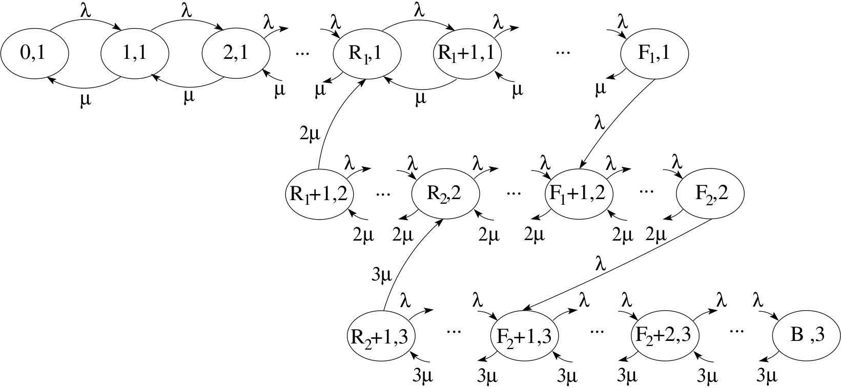
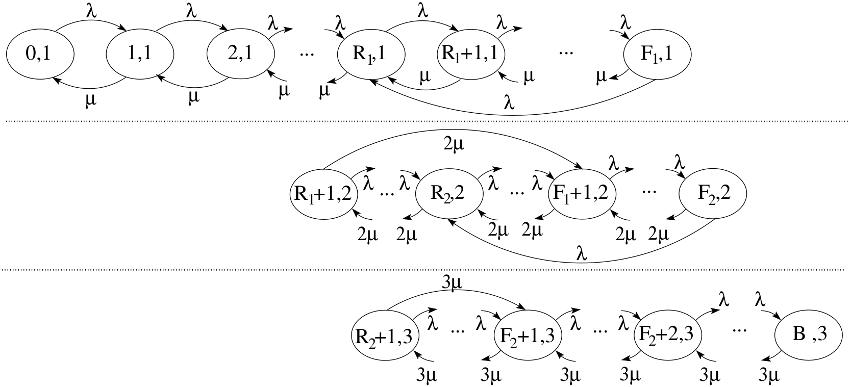
Figure 2: (a) Markov chain for K=3 ,        (b) Micro-chains aggregation

4.1.1 Costs

The global cost defined in Equation (1) can be rewritten for fixed $[F,R]$. We have:

$$\overline{C}_{[F,R]}^{\pi}~{}=~{}\sum\limits_{k=1}^{K}~{}~{}\sum\limits_{m=R_{k-1}+1}^{F_{k}}~{}\pi(m,k)\cdot\overline{C}(m,k)\,,$$ (3)

where $\pi(m,k)$ represents the stationary probability in state $(m,k)$. For a given state of the environment (number of requests, number of activated VMs), the cloud provider pays a cost:

$$\overline{C}(m,k)=C_{H}\cdot m+C_{S}\cdot k+C_{A}\cdot\lambda\cdot\mathds{1}_{m=F_{k},\;k<K}+C_{D}\cdot\mu\cdot\min\{m,k\}\cdot\mathds{1}_{m=R_{k-1}+1,\;2\leq k\leq K}\\ +C_{R}\cdot\lambda\cdot\mathds{1}_{m=B,\;k=K}\,.$$ (4)

4.2 Aggregation methods to compute the global cost

Solving the Markov chain quickly becomes complex when the number of levels $K$ increases. So we propose to apply the SCA (Stochastic Complement Analysis) method [7], based on a decomposition and an aggregation of the Markov chain. This approach allows a simplified computation of the exact stationary probability. The aim is to separate the $K$ levels of the considered Markov chain into $K$ independent sub-chains, called micro-chains and then to solve each of them independently. We then build the aggregated Markov chain which has $K$ states such that each state represents an operating level. This chain is called macro-chain.

Details about micro-chains and macro-chain

For any level $k$, such that $1\leq k\leq K$, the micro-chain is built from the initial Markov chain by keeping the transitions inside the same level. As for the transitions between states of different levels, they are deleted and replaced by new transitions inside the micro-chains from a leaving state to an entering state of the initial chain. Let us illustrate this in Fig. 2.a for initial chain and in Fig. 2.b for the micro-chains. Inside level 2, the transitions with rate $\lambda$ and those with rate $2\mu$ are kept, while the transitions between level 2 and level 1 and those between level 2 and level 3 are removed. The deleted transitions between levels 2 and 3 are replaced by a transition inside level $2$ between $(F_{2},2)$ and $(R_{2},2)$ with rate $\lambda$, and inside level $3$ by a transition between $(R_{2}+1,3)$ and $(F_{2}+1,3)$ with rate $3\mu$. Similarly for transitions between levels 2 and 1, then the process is generalised for any levels.

The macro-chain, is represented by a $K$ states Markov chain, such that each state is a level $k$ (with $1\leq k\leq K$). The macro-chain is a birth-death process for which computing the stationary probability is well-known. Let $\Pi$ be the stationary distribution of the macro-chain and $\pi_{k}$ be the stationary distribution of the micro-chain of level $k$ (with $1\leq k\leq K$). We denote by $\pi$ the stationary distribution of the initial Markov chain. From the SCA method, the probability distribution $\pi$ is computed as follows:

$$\forall~{}(m,k)\in\mathbb{S},\;\pi(m,k)~{}=~{}\Pi(k)\cdot\pi_{k}(m)\,.$$ (5)

Since, as pointed out in [31], the use of closed formulas suffers from numerical instability, the solving of Markov chains (micro and macro) is done numerically using the power method implemented in the marmoteCore software [33]. Each micro-chain is solved separately, next the macro-chain, and lastly, with Eq. 5, the initial Markov chain. The distributions obtained with the aggregation process are compared with those obtained by direct computations on the whole chain. The difference is always smaller than $10^{-8}$ which is the precision we choose for our computations.

Aggregated Costs

The aggregation framework described above, allows to compute the global cost $\overline{C}_{[F,R]}^{\pi}$, defined by Eq. (3), in an aggregated form based on the costs per level computed with micro-chains.

Theorem 1 (Aggregated Cost Function).

Let $[F,R]$ be fixed thresholds, then the expected cost $\overline{C}_{[F,R]}^{\pi}$ of the system can be decomposed as:

$$\overline{C}_{[F,R]}^{\pi}~{}=~{}\sum\limits_{k=1}^{K}~{}\Pi(k)\cdot\overline{C}(k)\,,\quad\text{ with }\,\,\overline{C}(k)=\sum\limits_{m=R_{k-1}+1}^{F_{k}}\pi_{k}(m)\cdot\overline{C}(m,k)\,,$$

where $\overline{C}(k)$ represents the expected cost of level $k$.

Proof.

We use Eq. (5) in Eq. (3) to get $\overline{C}_{[F,R]}^{\pi}=~{}\sum\limits_{k=1}^{K}~{}~{}\sum\limits_{m=R_{k-1}+1}^{F_{k}}~{}\pi_{k}(m)\cdot\Pi(k)\cdot\overline{C}(m,k)\,.$ Because $\Pi(k)$ does not depend on $m$, it is removed from the second sum. This yields the average aggregated costs per level weighted by the macro-chain stationary distribution.

$$\overline{C}_{[F,R]}^{\pi}~{}=~{}\sum\limits_{k=1}^{K}~{}\Pi(k)~{}\cdot\sum\limits_{m=R_{k-1}+1}^{F_{k}}~{}\pi_{k}(m)\cdot\overline{C}(m,k)~{}=~{}\sum\limits_{k=1}^{K}~{}\Pi(k)\cdot\overline{C}(k)\,.$$

∎

Theorem 1 suggests an efficient approach for the global cost computation. Indeed, instead of having computations on a multidimensional Markov chain, we have computations over several one-dimensional Markov chains. We take advantage of this aggregated expression to improve the computation of the expected cost when only a single threshold changes.

Corollary 2.

Let $[F,R]$ be a fixed vector of thresholds. It is assumed that the micro-chains and the costs per level associated with $[F,R]$ are already computed. The modification of a threshold $F_{k}$ or $R_{k}$ in $[F,R]$ only impacts the levels $k$ and $k+1$ in the Markov chain. Therefore, the computation of the new average cost only requires a new computation of $\pi_{k},\pi_{k+1},\overline{C}(k),\overline{C}(k+1)$ and $\Pi$.

The intuition about this corollary can be deduced from the transition graph in Fig. 2.a. When modifying $F_{2}$, it only impacts the distributions $\pi_{2}$ and $\pi_{3}$. We thus have to compute new $\overline{C}(2)$ and $\overline{C}(3)$, while the last expected cost $\overline{C}(1)$ remains unchanged. The details of the proof are below.

Proof.

Recall that we define the load of the system by $\rho=\lambda/\mu$. Using the balance equations in [7], we exhibit the impact generated by the modification of activation and deactivation thresholds on the stationary probability distributions of the micro-chains first and then of the macro-chain.

Impact on the micro-chains:  Owing to $m\in[R_{k-1}+1,F_{k}]$ for all $k\in\{1,\ldots,K\}$, we can therefore express the stationary probability of each state in the level $k$ by: $\pi_{k}(m)~{}=~{}\pi_{k}(R_{k-1}+1)\cdot\gamma_{m}^{k}$ where:

$$\pi_{k}(R_{k-1}+1)=\Biggl{(}\sum_{m=R_{k-1}+1}^{F_{k}}\gamma_{m}^{k}\Biggr{)}^{-1}\,,$$

and

$$\gamma_{m}^{k}=\begin{cases}\sum\limits_{j=0}^{m-R_{k-1}-1}\left(\dfrac{\rho}{k}\right)^{j}\,,~{}\mbox{ if }R_{k-1}+1\leq m\leq R_{k}\,;\\ \sum\limits_{j=0}^{m-R_{k-1}-1}\left(\dfrac{\rho}{k}\right)^{j}~{}-\gamma^{k}_{F_{k}}\cdot\sum\limits_{j=1}^{m-R_{k}}\left(\dfrac{\rho}{k}\right)^{j}\,,~{}\mbox{ if }R_{k}+1\leq m\leq F_{k-1}+1\,;\\ \sum\limits_{j=m-F_{k-1}-1}^{m-R_{k-1}-1}\left(\dfrac{\rho}{k}\right)^{j}~{}-~{}\gamma^{k}_{F_{k}}\cdot\sum\limits_{j=1}^{m-R_{k}}\left(\dfrac{\rho}{k}\right)^{j}\,,~{}\mbox{ if }F_{k-1}+2\leq m\leq F_{k}-1\,;\\ \rho\Bigg{[}\left(\dfrac{\rho}{k}\right)^{F_{k}-F_{k-1}}-\left(\dfrac{\rho}{k}\right)^{F_{k}-R_{k-1}+1}\Bigg{]}/\left(k+\rho\left(\dfrac{\rho}{k}\right)^{F_{k}-R_{k}}\right)\,,~{}\mbox{ if }m=F_{k}\,.\end{cases}$$

Note that $\pi_{k}(R_{k-1}+1)$ is determined through normalisation condition which states that the sum of probabilities of all states of the micro-chain of level $k$ equals 1.

We notice, in the equations above, that the stationary probability formulas of $\pi_{k}(m)$ of levels $k$ only depend on the thresholds $R_{k-1}$, $R_{k}$, $F_{k-1}$ and $F_{k}$. This shows that the variation of a threshold $R_{k}$ or $F_{k}$ has an impact only on levels $k$ and $k+1$ but not on the other levels. Moreover, since the micro-chain of level $k$ starts from state ($R_{k-1}+1,k$) and ends in state ($F_{k},k$), then thresholds from level $1$ to $k-2$ as well as thresholds from level $k+2$ to $K$ are not involved on the stationary distribution of the level $k$.

To resume, if we modify an activation threshold $F_{k}$, then it will modify states $(F_{k},k)$ and $(F_{k}+\!1,k\!+\!1)$ and the two micro-chains of level $k$ and $k+1$. If we modify, a deactivation threshold $R_{k-1}$, then it will modify states $(R_{k-1}+\!1,k)$ and $(R_{k-1},k-1)$ and the two micro-chains of levels $k-1$ and $k$.

Finally, the variation of a threshold from level $k$ modifies only the two micro-chains of level $k$ and $k+1$. Hence, to compute the cost with respect to Theorem 1 we only need to recalculate the stationary probabilities and thus the associated costs of these levels. The costs of the other levels are left unchanged.

Impact on the macro-chain:  A change in a threshold value modifies some transitions of the macro-chain. This can be seen, similarly as previously, using the balance equations: $\lambda_{k}~{}=~{}\lambda\cdot\pi_{k}(F_{k})$, $\forall~{}k~{}=~{}1,\ldots,K-1$, and $\mu_{k}~{}=~{}\mu\cdot\pi_{k}(R_{k-1}+1)$, $\forall~{}k~{}=~{}2,\ldots,K$. This gives the following formulas for the stationary probability distribution, for all $k\in\{2,\ldots,K\}$:

$$\begin{cases}\lambda_{k}~{}=~{}\lambda\cdot\pi_{k}(F_{k})\qquad\qquad\ \ \forall~{}k~{}=~{}1,\ldots,K-1\\ \mu_{k}~{}=~{}\mu\cdot\pi_{k}(R_{k-1}+1)\qquad\forall~{}k~{}=~{}2,\ldots,K\end{cases}\,.$$

∎

4.3 Thresholds calculation using stationary distributions of Markov chain

Our first approach relies on thresholds calculation using the stationary distribution of the underlined Markov chain coupled with an optimisation problem. We focus here on different static algorithms which compute the optimal threshold policy minimising the expected global cost.

The optimisation problem

For a set of fixed parameters: $\lambda$, $\mu$, $B$, $K$, and costs: $C_{a}$, $C_{d}$, $C_{h}$, $C_{s}$, $C_{r}$, the algorithms seeks to find the vector of thresholds $[F,R]$, such that the objective function is minimal. The objective function is the expected cost $\overline{C}_{[F,R]}^{\pi}$ defined by Eq.(3). For any solution $[F,R]$, the computation of the expected cost depends on the stationary distribution $\pi$ of the Markov chain $\{X(t)\}_{t\geq 0}$ induced by $[F,R]$. The thresholds must verify some given constraints resulting from the principle of hysteresis. That is: $R_{k}<F_{k}$, $R_{k-1}<R_{k}$ and $F_{k-1}<F_{k}$. Also, it is assumed that servers do not work for free. That is: $k<F_{k}$. Therefore, we have to solve the constrained optimisation problem given by:

$$\begin{aligned} &\underset{F,R}{\text{Minimise}}&&\hskip 28.45274pt\overline{C}_{[F,R]}^{\pi}\\ &\text{u.c.}&&R_{i}<F_{i}~{}~{}~{}\;i=1,\ldots,K-1.\\ &&&F_{1}<F_{2}<\cdots<F_{K-1}<B\\ &&&0\leq R_{1}<R_{2}<\cdots<R_{K-1}\\ &&&F_{i}~{},~{}R_{i}\in\mathbb{N}\end{aligned}\,.$$ (6)

Since the cost function is non-convex [9] and threshold values should be integer, we face up a combinatorial problem whose resolution time increases exponentially with the number of thresholds.

4.3.1 Local search heuristics

To solve this optimisation problem, several local search heuristics and one meta-heuristic have been developed in [9]. Most of the heuristics are inspired by Kranenburg et al. [27] which presents three different heuristics to resolve a lost sales inventory problem with, unlike us, only a single threshold by level. Actually usual base-stock heuristics had to be adapted to the hysteresis model as it is necessary to manage double thresholds now. The work [9] compares both the accuracy and execution time of these heuristics in numerical experiments. We keep here the two heuristics BPL, NLS that have the best results and present some improvement ways.

Best Per Level (BPL)

This algorithm first initialises $[F,R]$ with the lowest feasible value, i.e. $F_{1}=1,F_{2}=2,...,F_{K-1}=K$ and $R_{1}=0,R_{2}=1,...,R_{K-1}=K-1$. Then it improves each threshold in the following order: it starts with the first activation threshold $F_{1}$ by testing all its possible values taking into account the hysteresis constraints. A new value of $F_{1}$ that improves the global cost, will replace the old one. Then, it will move on to $F_{2}$, $F_{3}$, … , $F_{K-1},R_{1},R_{2},...,R_{K-1}$. Once a loop is finished, it will restart again until the mean global cost is not improved anymore.

Neighborhood Local Search (NLS)

This algorithm is the classical local search algorithm. We randomly initialise the solution $[F,R]$. Then we generate the neighborhood $\mathcal{V}(x)$ of a current solution $x$. Each neighboring solution is the same as the current solution except for a shift $\pm 1$ for one of the thresholds. The algorithm explores all the neighborhood and returns the best solution among $\mathcal{V}$. Again, it loops the same process until the mean global cost is not improved anymore.

4.3.2 Aggregation for local search algorithms

Local search algorithms are based on an exploration step in a set of feasible solutions that must be evaluated. This evaluation consists of calculating $C^{\pi}_{([F,R])}$. From Section 4.2, this computation depends on the stationary distributions $\pi_{k}$ of the micro-chains, on the distribution $\Pi$ of the macro-chain, and on the costs per level. Although, the neighboring solutions differ from the current solution only by a single change of one of their thresholds, after any modification we have to recalculate all these elements. This requires a huge amount of time which depends on the number of neighboring solutions tested at each iteration and which increases when we consider large scale scenarios (with large $K$ and $B$).

We ensure the algorithms to avoid so many computations for each neighboring solution with Corollary 2. Its use will widely accelerate the algorithm without altering the accuracy. Indeed, at each iteration, we only have to compute the stationary distributions and the corresponding average costs per level of the two micro-chains impacted by a change of a threshold. We no longer need to compute the distributions of the other micro-chains since we can keep their average costs per level. The macro-chain still need to be solved however.

Although decomposition and aggregation approaches reduce the number of computations to perform, some algorithmic tricks must be implemented in order to ensure a proper and efficient running. Hence, the two micro-chains of the current solution that are modified when we study a neighborhood, have to be stored since they will be reused many times. By this way, the execution time of aggregated local search heuristics is reduced. This will be all the more effective when $K$ increases.

4.3.3 Solution using queueing model approximations.

We work here on a new heuristic which calculates a near-optimal solution very quickly. It can be considered as a method in its own right but can be also used for the initialisation step in local search heuristics. This heuristic is called MMK approximation since it uses ${M}/{M}/{k}/{B}$ results to compute costs of these fairly close models.

Principle of the heuristic

The main idea of the heuristic is that, at each level $k$, we compute an approximation of the mean global cost by using the stationary distribution of the Markov chain of a $M/M/k/B$ queue model instead of using the Markov chain of Section 4.1. In such queues, the stationary distribution of the Markov chain is given by a closed formula. Thus, the computation of the distribution is done in a constant time due to the closed formula while the exact computation is much longer. Hence, we obtain an approximate solution of the expected cost very quickly. In order to find the best threshold $m$ for which it is better to activate or deactivate, we proceed by comparing approximated costs of having $k$ VMs activated with the one of having $k+1$ (respectively $k-1$) VMs activated added by the activation (respectively deactivation) cost.

Design of the heuristic

Let us recall, the formulas of the stationary distributions in $M/M/k/B$ queues. Let $\hat{\pi}(k,m)$ be the stationary distribution of state $(m,k)$, we get:

$$\hat{\pi}(k,m)=\hat{\pi}(k,0)\cdot\dfrac{\rho^{m}}{m!}\,\ \mbox{ for }1\leq m\leq k\quad\mbox{ and }\quad\hat{\pi}(k,m)=\hat{\pi}(k,0)\cdot\dfrac{a^{m}\cdot k^{k}}{k!}\,\ \mbox{ for }k<m\leq B.$$

where $\rho=\dfrac{\lambda}{\mu}$, $a=\dfrac{\rho}{k}<1$ and where $\hat{\pi}(k,0)$ is:

$$\hat{\pi}(k,0)\!=\!\Bigg{(}\sum_{m=0}^{k-1}\dfrac{\rho^{m}}{m!}+\dfrac{k^{k}}{k!}(B-k+1)\Bigg{)}^{\!-1}\mbox{ if }a=1\ \mbox{and}\ \hat{\pi}(k,0)\!=\!\Bigg{(}\sum_{m=0}^{k-1}\dfrac{\rho^{m}}{m!}+\dfrac{\rho^{k}}{k!}\dfrac{1-a^{B-k+1}}{1-a}\Bigg{)}^{\!-1}\mbox{ if }a\neq 1.$$

Let us define $\hat{C}_{k}(m)$ as the approximate cost of having $k$ VMs turned on and $m$ requests in the system by:

$$\hat{C}_{k}(m)=\hat{\pi}(k,m)\bigl{(}m\cdot C_{H}+k\cdot C_{S}\bigr{)}+\hat{\pi}(k,B)\cdot\lambda\cdot C_{R}\,;$$

define $\hat{C}^{A}_{k+1}(m)$ as the approximate cost of having $m$ requests in level $k+1$ knowing that we have just activated a new VM by:

$$\hat{C}^{A}_{k+1}(m)=\hat{\pi}(k+1,m)\bigl{(}m\cdot C_{H}+(k+1)\cdot C_{S}\bigr{)}+\hat{\pi}(k+1,B)\cdot\lambda\cdot C_{R}+\hat{\pi}(k,m-1)\lambda C_{A}\,.$$

Let us define $\hat{C}^{D}_{k}(m)$ as the approximate cost of having $m$ requests in level $k$ knowing that we have just deactivated a new VM by:

$$\hat{C}^{D}_{k}(m)=\hat{\pi}(k,m)\left(mC_{H}+kC_{S}\right)+\hat{\pi}(k,B)\lambda C_{R}+\hat{\pi}(k+1,m+1)(k+1)\mu C_{D}\,.$$

We want to compare these costs to know whether we should activate, deactivate or let the servers unchanged.

For the activation thresholds. We define $\phi^{A}_{k}(m)=\hat{C}_{k}(m)-\hat{C}^{A}_{k+1}(m)$. If $\phi^{A}_{k}(m)<0$ then it is better to not activate a new server while if $\phi^{A}_{k}(m)\geq 0$ it is better to activate a new one. There is no evidence of the monotonicity of $\phi^{A}_{k}(m)$ in $m$, nevertheless we choose the threshold by $F_{k}=\min\left\{m:\phi^{A}_{k}(m)\geq 0\right\}$. To compute the whole thresholds, all $k$ are studied in an ascending order. For a fixed level $k$, we need to compute $\phi^{A}_{k}(m)$ for all $m$ and stop when the function $\phi^{A}_{k}(m)$ is larger than $0$.

For deactivation thresholds. We define $\phi^{D}_{k}(m)=\hat{C}_{k+1}(m)-\hat{C}^{D}_{k}(m)$. If $\phi^{D}_{k}(m)<0$ then it is better to stay with $k+1$ servers while if $\phi^{D}_{k}(m)\geq 0$ it is better to deactivate a virtual machine. Similarly, there is no evidence about the monotonicity of $\phi^{D}_{k}(m)$ but we define $R_{k}=\min\left\{m:\phi^{D}_{k}(m)\geq 0\right\}$. The computation of the whole deactivation thresholds is similar to the activation ones.

Markov chains approximation methods coupled with local search heuristics

The initialisation of the local search heuristics presented in 4.3.1 either is totally random or simply chooses the bounds (lowest values or highest values) of the solution space. The aim here is to improve the speed and the accuracy of these heuristics by coupling them with the MMKB approximation used as an initialisation step. This initialisation aims at finding an initial solution that will be in the basin of attraction of the optimal solution. Starting with this solution improves the ability of local search algorithms to reach the best solution in a faster time. This new method behaves better than the initialisation based on Fluid approximation adapted from [17] in the work [9]. We define by Alg MMK the coupled heuristic with MMKB approximation.

5 Computing policies with Markov Decision Process

We consider here the multi-server queue of Section 3.1 and the controlled model in which only a single virtual resource can be activated or deactivated at a time decision. This optimal control problem is a continuous time process and thus should be solved using a Semi Markov Decision Process (SMDP). In this section, we first describe the uniformised SMDP and its solving. Then we underline the differences between the optimal control model and the optimisation problem of Section 4.3.

5.1 The SMDP model

5.1.1 Elements of the SMDP

The state space is the one defined in Section 3: $\mathcal{S}=\{0,1,\ldots,B\}\times\{1,\ldots,K\}$. Hence, a state $x\in\mathcal{S}$ is such that $x=(m,k)$ where $m$ is the number of customers in the system and $k$ the number of active servers. Similarly, the action space ${{\cal{A}}}~{}=~{}\{-1,0,1\}$ represents respectively: deactivate one machine, left unchanged the active servers, or activate one machine.

The system evolves in continuous time and at some epoch a transition occurs. When a transition occurs, the controller observes the current state and reacts to adapt the resources by activating or deactivating the virtual machines. The activation or deactivation are instantaneous and then the system evolves until another transition occurs. Two events can occur: an arrival with rate $\lambda$ which increases the number of customers present in the system by one or a departure which decreases the number of customers by one.

Let $x=(m,k)$ be the state and $a$ the action, we define $N(k+a)$ as the real number of active VM after the action $a$ was triggered. We have $N(k+a)=\mathrm{min}\{\mathrm{max}\{1,k+a\},K\}$. It follows that the transition rate is equal to

$$\begin{cases}\lambda&\text{if }y=\!\bigl{(}\mathrm{min}\{m\!+\!1,B\},N(k+a)\bigr{)}\\ \mu\!\cdot\!\min\{m,N(k\!+\!a)\}&\text{if }y=\!\bigl{(}\mathrm{max}\{0,m-\!1\},N(k+a)\bigr{)}\end{cases}.$$

5.1.2 Uniformised transition probabilities

We apply here the standard method to deal with continuous time MDP: the uniformisation framework. We follow the line of chapter 11 of [32] to define the uniformised MDP.

We define $\Lambda(m,k,a)$ as the rate per state. We have $\Lambda(m,k,a)=\lambda+\mu\!\cdot\!\min\{m,N(k+a)\}$. From now on, any component denoted by "$\sim$" refers to the uniformised process. We thus define the uniformisation rate by $\tilde{\Lambda}$ with $\tilde{\Lambda}=\max_{(m,k,a)}\Lambda(m,k,a)=\lambda+K\mu$ which is the maximum transition rate. The transition probability from state $x$ to state $y$ when action $a$ is triggered is denoted by $\tilde{p}(y|x,a)$ in the uniformised model.

We have:

$$\tilde{p}(y|x,a)=\begin{cases}\dfrac{\lambda}{\tilde{\Lambda}}&\text{if }y=\left(m+1,N(k+a)\right)\\ \dfrac{\mu\min\{m,N(k+a)\}}{\tilde{\Lambda}}&\text{if }y=\left(m-1,N(k+a)\right)\\ \dfrac{\tilde{\Lambda}-\Lambda(m,k,a)}{\tilde{\Lambda}}&\text{when }y=(m,k)\\ 0&\text{otherwise}\,,\end{cases}$$

when $x=(m,k)$ such that $0<m<B$ and $a$ is arbitrary ; when $x=(B,k)$ with $a\not=0$, or when $x=(B,k)$ with $k\not=K$ and $a\not=+1$ or also when $x=(B,k)$ with $k\not=1$ and $a\not=-1$; when $x=(1,k)$ with $a\not=0$, or when $x=(1,k)$ with $k\not=K$ and $a\not=+1$, or also when $x=(1,k)$ with $k\not=1$ and $a\not=-1$. We have:

$$\tilde{\Lambda}\times\tilde{p}(y|x,a)=\begin{cases}\mu\min\{m,N(k+a)\}&\text{if }y=\left(B-1,N(k+a)\right)\\ \tilde{\Lambda}-\mu\min\{m,N(k+a)\}&\text{when }y=(B,k)\\ 0&\text{otherwise}\,,\end{cases}$$

when $x=(B,k)$ with $a=0$, or when $x=(B,k)$ with $k\not=K$ and $a\not=+1$, or also when $x=(B,k)$ with $k\not=1$ and $a\not=-1$. We have

$$\tilde{\Lambda}\times\tilde{p}(y|x,a)=\begin{cases}\lambda&\text{if }y=\left(1,N(k+a)\right)\\ \tilde{\Lambda}-\lambda&\text{when }y=(0,k)\\ 0&\text{otherwise}\,,\end{cases}$$

when $x=(0,k)$ with $a=0$, or when $x=(0,k)$ with $k\not=K$ and $a\not=+1$, or when $x=(0,k)$ with $k\not=1$ and $a\not=-1$.

5.1.3 The uniformised stage costs

We take the definition of costs of Section 3.1. Instantaneous costs are charged only once and are related to activation, deactivation and losses. Accumulated costs are accumulated over time and are related to consumption and holding cost. After uniformisation of instantaneous and accumulated costs (Chapter 11.5 of [32]), we obtain the following equation for $x=(m,k)$:

$$\tilde{c}(x,a)=\bigl{(}C_{A}\mathds{1}_{\{a=1\}}+C_{D}\mathds{1}_{\{a=-1\}}\bigr{)}\dfrac{\Lambda(x,a)}{\tilde{\Lambda}}+\dfrac{\lambda}{\tilde{\Lambda}}C_{R}\mathds{1}_{\{m=B\}}+\dfrac{1}{\tilde{\Lambda}}\bigl{(}N(k+a)\cdot C_{S}+m\cdot C_{H}\bigr{)}\,.$$

Objective function

The objective function defined in Equation (1) translates for all $x\in\mathcal{S}$ into

$$\rho^{\pi}(x)=\lim_{N\rightarrow\infty}E^{\pi}\Bigl{[}\dfrac{1}{N}\sum\limits_{t=0}^{N-1}\tilde{c}(x_{t},\pi(x_{t}))~{}|~{}x_{0}=x\Bigr{]}\,,$$

for a given policy $\pi$. The value $\rho^{\pi}$ is the expected stage cost and equals $\bar{C}$ when actions follow policy $\pi$.

5.2 Solving the MDP

5.2.1 Classification of the SMDP

Our SMDP is an average cost model. This is why, the expected stage costs depend on the recurrent properties of the underlying Markov chain that is generated by a deterministic policy. A classification is then necessary to study them. We use the classification scheme of [32].

Definition 6 (Chapter 8.3.1 in [32]).

A MDP is:

1. Unichain if, the transition matrix corresponding to every deterministic stationary policy is unichain, that is, it consists of a single recurrent class, plus a possibly empty set of transient states;

2. Multichain if, the transition matrix corresponding to at least one deterministic stationary policy contains two or more recurrent classes;

3. Communicating if, for every pair of state $x$ and $y$ in ${\cal S}$, there exists a deterministic stationary policy $\pi$ under which $y$ is accessible from $x$, that is, $p_{\pi}^{n}(y,x)>0$ for some $n\geq 1$;

Proposition 2.

The MDP is multichain. There is a stationary deterministic policy with monotone hysteresis properties that induces a corresponding Markov chain with more than two different recurrent classes.

Proof.

We assume that $K\geq 2$ and let $k$ be such that $k\in[1,\ldots,K]$. We define the policy $q$ as follows. For any level $l$ with $l<k-1$, we have only activation. There exists $m\in[0,\cdots,B]$ such that $q(m^{\prime},l)=1$ for any $m\leq m^{\prime}$ and $q(m,l)\leq q(m,l-1)$. For level $k$ we have neither activation nor deactivation and $q(m,k)=0$ for all $m\in[0,\cdots,B]$. For any level $l$ with $l>k+1$, we have only deactivation. There exists $m\in[0,\cdots,B]$ such that $q(m^{\prime},l)=-1$ for any $m^{\prime}\leq m$ and $q(m,l)\geq q(m,l+1)$. Therefore, we have three recurrent classes: the level $k$, the level $k-1$ and the level $k+1$ (and two recurrent classes for $K=2$). See supplementary materials in appendix B. ∎

Lemma 3.

The MDP is communicating. There exists a stationary isotone hysteresis policy such that the corresponding Markov chain is irreducible.

Proof.

We exhibit such a policy. Let $\pi$ be the deterministic stationary policy such that the thresholds $l_{k}$ are defined by $l_{k}=0$ and the thresholds $L_{k}$ by $L_{k}=B$ for all $k$. The induced Markov chain is irreducible since any level can be reached from another one (when $m=0$ or $m=B$) and since in a given level all the states are reachable from any state. Thus, we have that $p_{\pi}^{n}(y,x)>0$ for some $n\geq 1$ for all couples $(x,y)$. Therefore the MDP is communicating. ∎

Bellman Equations

In the multichain case, the Bellman Equations are composed by two equations. In the uniformised model, we then have ([32]) the two following optimality equations:

$$\min_{a\in A}\Bigg{\{}\sum\limits_{y\in{\cal{X}}}\tilde{p}(y\,|\,x,a)\rho(y)-\rho(x)\Bigg{\}}=0\ \text{ and }\ U(x)=\min_{a\in B_{x}}\Bigg{\{}\tilde{c}(x,a)-\dfrac{\rho(x)}{\tilde{\Lambda}}+\sum\limits_{y\in{\cal{X}}}\tilde{p}(y\,|\,x,a)\cdot U(y)\Bigg{\}}$$

for all $x\in{\cal{X}}$, where

$$B_{x}=\Big{\{}a\in{{\cal{A}}}~{}\big{|}~{}\sum\limits_{y\in{\cal{X}}}\tilde{p}(y\,|\,x,a)\rho(y)~{}=~{}\rho(x)\Big{\}}\,.$$

It could be noticed that in the unichain case, $B_{x}~{}=~{}{{\cal{A}}}$ and that the two equations reduce to only the second one. These two non linear equation systems should be numerically solved to find $U(x)$ and $\rho(x)$. Once these terms are approximated we deduce the optimal policy with:

$$q(x)=\arg\min_{a\in B_{x}}\bigg{\{}\tilde{c}(x,a)+\sum\limits_{y\in{\cal{X}}}\tilde{p}(y\,|\,x,a)\cdot U(y)\bigg{\}}\,.$$

5.2.2 Algorithms

We describe here the choice of the algorithms used to solve this multichain and communicating model. Computing multichain model is much complicated namely since testing if an induced Markov chain is unichain is a NP complete problem. We first show that we actually can use some unichain algorithms due to the communicating properties of our SMDP, then we present two structured algorithms based on hysteresis properties.

Unichain algorithms

From [32] it exists a multichain policy iteration algorithm that solves multichain models. It requires to solve two equation systems and thus is time consuming. However, by Proposition 3, our MDP is communicating and in Theorem 8.3.2 of [32] it is proved that unichain value iteration algorithm converges to the optimal value in communicating models. This property allows us to use the unichain value iteration algorithm.

There is also, in [32], a policy iteration algorithm for communicating models. It requires to start with an initial unichain policy and its inner loop roughly differs from the unichain case in order to keep some properties. We decide to use here algorithms based on unichain policy iteration. There does not exist theoretical guarantee of their convergence, but we showed in numerical experiments that they always converge to the same policy than value iteration.

Four different usual unichain algorithms will be considered: Value Iteration, Relative value iteration, Policy Iteration modified and Policy Iteration modified adapted, which adapts its precision in the policy evaluation step. They are respectively referred by VI, RVI, PI and PI Adapt. The algorithms are all described in [32] and are already implemented in the software [33].

Structured Policies algorithm

We now integrate hysteresis properties in the algorithms. Two classes of policies have been investigated: Double Level class (Definition 1) and Monotone Hysteresis class (Definition 4). The goal is to plug hysteresis assumptions during the policy improvement step of policy iteration (Policy Iteration has two major steps). This allows to test less actions at each iteration and to speed up the algorithm. Two algorithms are implemented: one for the double level properties (referred as DL-PI) and one for the hysteresis properties (referred as Hy-PI).

On the other hand, we do not have theoretical guarantee that these methods converge, first because we do not theoretically know if hysteresis policies are optimal for our model, and second because the underlying PI also has no convergence guarantees in multichain. Nevertheless, in the numerical experiments we made (see later) all the optimal policies returned by classical algorithms have hysteresis properties. Furthermore, all MDP algorithms considered here (structured as well as classical) returned the same solution. This therefore underlines the interest of considering such hysteresis policies especially since the gain in running time is obvious as observed in the experiments.

Computation of the hysteresis thresholds

The non-structured MDPs (also called simple MDPs) do not assume any restrictions for their policy research. Thus, they return the optimal policy and so return a decision rule $q^{*}$ which gives the optimal action to take but not the thresholds. Therefore, we need to test the hysteresis property and to compute the $l$ and $L$ hysteresis thresholds consistently with Definition 4. Let $q^{*}$ be the optimal policy returned by the PI algorithm. We check if $q^{*}$ is monotone, if not the optimal policy is not hysteresis. If so, we proceed as follows. We consider, for all $k$, the set $\{m\mid q^{*}(m,k)=1\text{ and }q^{*}(m-1,k)=0\}$. If the set is of size $2$ then the policy is not hysteresis else it is hysteresis. In hysteresis case, if the set is of size $1$ then $L_{k+1}=m$ and if the set is empty then $L_{k+1}=\infty$. Also, we consider, for all $k$, the set $\{m\mid q^{*}(m+1,k)=0\text{ and }q^{*}(m,k)=-1\}$. If the set is of size $2$ then the policy is not hysteresis, else it is. If the set is of size $1$ then $l_{k+1}=m$ and if the set is empty then $l_{k+1}=0$.

5.3 Theoretical comparison between the two approaches MC and MDP

Although they seem very similar these two models present some rather subtle theoretical differences with notable consequences. They are studied here while the numerical comparisons will be carried out in Section 7.

5.3.1 Number of activated resources

A major difference between the two approaches is related to the class of policy they consider and the consequences on the management of resources. The (MC) approach (Section 4), deals with strictly isotone policies (i.e. $0=l_{1}<l_{2}<\ldots<l_{K}\leq B$ and $0=L_{1}<L_{2}<\ldots<L_{K}\leq B$). Therefore, $L_{K}$ can not be infinite, and in this model all the $K$ servers should be activated. Furthermore, since inequalities are strict $l_{K}\geq K$, the only state in which there is only one active server is restricted to the level $k=1$. Strictly isotone assumption is required to keep the size of the chain constant (see [30]). On the other hand, the (MDP) approach either does not assume any structural property on the policy or considers isotone policy (see Definition 3). In this approach constraints are looser and it is possible not to have all the servers activated and conversely to have many resources activated even if the queue is empty.

The resource management follows the optimal policies returned by each of the approaches. Three categories of resource management have been identified. We noticed that these categories depend on the relative values of the parameters ($\lambda,\mu$) between them. However, we do not know how to precisely quantify their borders.

Definition 7.

These categories are:

1. Medium arrival case: All VMs are turned On and turned Off in both approaches. This occurs when the system load is medium, i.e. the arrival rate $\lambda$ is close to the service rate $k\times\mu$.

2. Low arrival case: All VMs are turned On and turned Off in (MC) while in (MDP) some VMs will never be activated. This occurs when the system load is low, i.e. the arrival rate $\lambda$ is very small compared to the service rate $k\times\mu$.

3. High arrival case: All VMs are turned On and turned Off in (MC) while in (MDP) some VMs will never be deactivated. This occurs when the system load is high, i.e. the arrival rate $\lambda$ is very large compared to the service rate $k\times\mu$.

Proposition 3 (Non optimality of strictly isotones policies).

The above classification helps us to claim that strictly isotone policies are not optimal and that MDP approach performs better.

Proof.

During the numerical experiments in Section 7, we identify numerous cases in which strictly isotone policies are not optimal. This is mainly due to the phenomenon of non activation or non deactivation exposed above: examples of non-optimality are found in both low arrival and high arrival categories. The structured (MDP)s have less constraints and return the optimal solution which is the one computed by simple MDPs. See appendix A for details. ∎

The proposition above highlights another benefit of MDP approaches since they allow to size the exact number of machines to be activated (this is particularly true in the low arrival case). Hence, if in a policy resulting from a MDP there exits a $k$ such that for all $l>k$ and for all $m\in\{1,\ldots,B\}$ we have $q(m,l)<1$, then $K-k$ machines are not necessary. This is not true in MC heuristics, nevertheless, it is possible to adapt the previous heuristics to find the optimal number of VM to be activated in low arrival case. This requires running the algorithms for each level $k$ with $k\in\{1,\ldots,K\}$. Then take the level $k$ which has the smallest cost says $k^{*}$. If $k^{*}=K$ all machines must be turned on in $K$, otherwise only $k^{*}$ machines are important and the other ones useless. But this method is time consuming. Also, such an adaptation for high arrival cases is not obvious.

5.3.2 Different temporal sequence of transitions

The last point to investigate is the difference in dynamical behavior between transitions. This difference is slight and has no effect on average costs, nevertheless it induces a difference on the values of the thresholds. In this system, there are two kinds of transitions: natural transitions which are due to events (departures or arrivals) and triggered transitions which are caused by the operator (activation or deactivation). These two transitions are instantaneous. Due to their intrinsic definitions, the models considered here do not observe the system at the same epochs. Hence, in the Markov chain the system is observed just before a natural transition while in the MDP the system is observed just after a natural transition. More formally, let us assume that $x$ is the state before a natural transition: it is seen by the Markov chain. Then the transition occurs and the state changes instantaneously in $x^{\prime}$ that is the state seen by the MDP. The controller reacts and the triggered transition occurs, thus the system moves in $x^{\prime\prime}$ in which the system remains until the next event which will cause the next natural transition. Since state changes are instantaneous, this has no impact on costs. See appendix B for details.

In the medium case arrival defined by Definition 7, thresholds are fully comparable and we have the following lemma

Lemma 4.

In the medium case arrival, hysteresis thresholds of Markov chain and SMDP hysteresis threshold can be inferred from each other. Let $(F_{1},\ldots,F_{K-1})$ and $(R_{1},\ldots,R_{K-1})$ be the thresholds of the MC model and let $(L_{2},\ldots,L_{K})$ and $(l_{2},\ldots,l_{K})$ be the SMDP thresholds. Then, for all $k\in\{1,\ldots,K-1\}$, we have: $L_{k+1}-1=F_{k}\quad\text{ and }\quad l_{k+1}+1=R_{k}.$

Proof.

We make the proof for an activation threshold. Let assume that the state just before a transition is $x=(F_{k},k)$, if an arrival event occurs then the system moves instantaneously in a state $x^{\prime}=(F_{k}+1,k)$. According Definition 5, a virtual machine is activated and then the system instantaneously moves again in $x^{\prime\prime}=(F_{k}+1,k+1)$. Observe now, that the state $x^{\prime}$ (according Definition 2) is the state in which the SMDP observes the system an takes its activation decision. Thus, we have $L_{k+1}=F_{k}+1$. The proof works similarly for deactivation. ∎

6 Real model for a Cloud provider

Now we are going to give real environment values to our models. The approach is difficult since, up to our knowledge, it does not exist, in the literature, an unified model including both energy, quality of service, and real traffic parameters. We propose to build a global cost taking into account both real energy consumption, real financial costs of virtual machines and Service Level Agreement (SLA) simultaneously from separate works. We think that the model presented is sufficiently generic to represent a large class of problems and is enough to give a relevant meaning to all parameters. With our algorithms and this model the cloud owner can generate meaningful optimised costs in real cases. Parameter values used in experiments can be found in Section 7.3.

6.1 Cost-Aware Model with energy consumption traces and real prices

Measurements of energy consumption

Many measurements are performed on the real datacenter grid5000 in [4], and energy consumption data are obtained for VMs hosted on physical servers in [13]. We keep these values in Watt for energy consumption of virtual machines.

Financial Cost

In order to keep the relevance of our cost-aware model, we must represent a financial cost. Henceforth, we transform energy consumption given in Watts into a financial cost based on the price in euros of the KWh in France fixed by national company. To obtain the financial values of the other prices, we observe the commercial offers of providers [34]. This gives us the operational costs.

Service Level Agreement

We propose to modify the performance part of our cost function for capturing the realistic scheme of the Service Level Agreement. Actually, we have to give a concrete meaning to our holding cost since it does not translate directly from usual SLA models. Indeed, in SLA contracts, it could be stated that when the response time exceeds a pre-defined threshold $T_{SLA}$ then penalty costs must be paid. Here, the penalty $C_{p}$ is the price that a customer pays for one hour of service of a virtual machine (full reimbursement) [34] and the threshold corresponds to a maximal time to process a request.

With our model, it is possible to define an holding cost that models the penalty to pay when the QoS is not satisfied. We focus on the mean response time in the system where the response time is denoted by $R_{T}$. The SLA condition translates in: $E[R_{T}]\leq T_{SLA}$. We introduce the mean number of customers $E(N)$ and with Little’s law we get: $E[N]\leq T_{SLA}\cdot\lambda$. We thus may define a customer threshold $N_{SLA}$ such that $N_{SLA}~{}=~{}T_{SLA}\cdot\lambda$. This customer threshold is the maximum number of requests, that the system can accept to keep the required QoS satisfied. Therefore, each time $m>N_{SLA}$, the cloud provider will pay a holding cost penalty of $C_{p}$ per customer.

Global cost formula

We obtain the expected global cost charged to the cloud provider:

$$\overline{C}(m,k) =C_{p}\cdot(m-N_{SLA},0)^{+}+C_{S}\cdot k+C_{p}\cdot\lambda\cdot\mathds{1}_{\{m=B,k=K\}}+C_{A}\cdot\lambda\cdot\mathds{1}_{\{m=F_{k},\,k<K\}}$$

$$\qquad+\>C_{D}\cdot\mu\cdot\min\{m,k\}\cdot\mathds{1}_{\{m=R_{k-1}+1,\;2\leq k\leq K\}}+C_{static}\,,$$

In the energy consumption part, $C_{static}$ represents the static financial cost derived from the idle energy consumption of the physical server which hosts the virtual machines. The remaining energy part of the cost function is left unchanged with the activation, deactivation, and energy costs of a VM defined above.

6.2 Real packet traffic and CPU utilisation

For obtaining concrete values of parameters $\lambda$ and $\mu$ we must search workload traces with real scenarios in public cloud. Here the traces come from MetaCentrum Czech National Grid data [35].

7 Numerical experiments

This part is devoted to numerical experiments and the comparison between all previous algorithms. We have implemented all methods in C++, with the stand-alone library [33].

7.1 Experiments design and results

All the experiments were carried out on a platform built on an Intel Xeon X7460 processor, with $6\times 4$ cores at $2,66$GHz and $16$ GB of RAM. Numerical experiments have been done for different Cloud model parameters. System parameters were taken arbitrarily. We defined four scenarios with different scales: Scenario A: K=3, B=20; Scenario B: K=5, B=40; Scenario C: K=8, B=60; Scenario D: K=16, B=100. We call Instance a set of parameters $\lambda,\mu,C_{a},C_{d},C_{h},C_{s},C_{r}$. The algorithms have been launched on $46656$ instances. Costs ($C_{a},C_{d},C_{h},C_{s}$) were taking values in $[0.5,1,2,5,10,20]$, $C_{r}$ in $[1,10,100,1000,5000,10000]$, queueing parameters $\lambda,\mu$ in $[0.5,1,2,5,10,20]$. We rank the different algorithms by assessing their accuracy and their running time. We first studied numerical experiments in the (MC) approach by comparing the different heuristics by these two criteria. For Scenario A, accuracy is computed based on optimal solution generated by exhaustive search. For higher scale scenarios (B,C,D), we compute accuracy regarding the best solution among the heuristics. Then, we compared all the (MDP) algorithms with the value iteration solution (convergence is known from Section 5.2.2) before comparison with the heuristics to compare both approaches. We finally ran the experiments for a concrete cloud scenario with real data, showing how we can effectively benefit from the best methods to calculate optimal thresholds.

Models	Algorithms	Scenario A		Scenario B		Scenario C		Scenario D
		Time (sec)	% Opt	Time (sec)	% Min	Time (sec)	% Min	Time (sec)	% Min
MC Heuristics	BPL	0,063 sec	96,9 %	2,684 sec	86,81%	37,23 sec	79,57 %	757 sec	55,39%
	BPL Agg	0,047 sec	96,9 %	1,163 sec	86,81%	10,27 sec	79,57 %	186 sec	55,39%
	BPL-MMK Agg	0,036 sec	97,78 %	0,53 sec	96,59 %	5,16 sec	95,39 %	31,7 sec	87,24 %
	NLS	0.043 sec	92,70 %	1,007 sec	62,24 %	12,38 sec	43,51 %	257 sec	20,44 %
	NLS Agg	0,034 sec	92,70 %	0,458 sec	62,24 %	4,05 sec	43,51 %	61 sec	20,44 %
	NLS-MMK Agg	0,014 sec	96,32 %	0,06 sec	93,58 %	0,9 sec	89,54 %	8,39 sec	76,17 %
MDP		Time (sec)	% Opt	Time (sec)	% Opt	Time (sec)	% Opt	Time (sec)	% Opt
	VI	0.0057 sec	100 %	0.021 sec	100 %	0.0406 sec	100 %	0,0944 sec	100 %
	RVI	0.0057 sec	100 %	0.021 sec	100 %	0.0406 sec	100 %	0,095 sec	100 %
	PI	0.0028 sec	100 %	0.0124 sec	100 %	0.0214 sec	100 %	0.0606 sec	100 %
	PI Adapted	0,0023 sec	100 %	0,0117 sec	100 %	0,0201 sec	100 %	0,0583 sec	100 %
	DL-PI	0,00115 sec	100 %	0,0072 sec	100 %	0,0105 sec	100 %	0,0452 sec	100 %
	Hy-PI	0,00113 sec	100 %	0,0069 sec	100 %	0,0100 sec	100 %	0,0442 sec	100 %
Comparison		Time (sec)	% Opt	Time (sec)	% Opt	Time (sec)	% Opt	Time (sec)	% Opt
	NLS-MMK Agg	0,014 sec	64,82 %	0,06 sec	61,52 %	0,9 sec	59,82 %	8,39 sec	52,61 %
	BPL-MMK Agg	0,036 sec	65,15 %	0,53 sec	62,65 %	5,16 sec	61,69 %	31,7 sec	57,1 %
	DL-PI	0,00115 sec	100 %	0,0072 sec	100 %	0,0105 sec	100 %	0,0452 sec	100 %
	Hy-PI	0,00113 sec	100 %	0,0069 sec	100 %	0,0100 sec	100 %	0,0442 sec	100 %

Table 1: Numerical experiments for comparison of heuristics and MDP algorithm

7.2 Experiments analysis

We display in Table 1 the comparisons for (MC) heuristics and (MDP) algorithms. For each algorithm, we display for each scenario the running time in seconds in the first column and the accuracy in the second column.

7.2.1 Assessing heuristics approaches

We want to assess the selected heuristics of [9] and the gain of the improvements proposed.

Aggregation strongly improves algorithms time speed

For the same efficiency, we first observe a significant time saving provided by the aggregation technique. As expected, the improvement in Scenario A is small, but the gain increases as the size of the system rises. Henceforth the execution time is divided by about $1.3$ when $K=3$ and $B=20$ and by about $3.8$ when $K=16$ and $B=100$ (e.g. BPL algorithm passes from 757 seconds to 186 seconds).

Impact of the M/M/k/B approximation

Coupled with heuristics BPL and NLS, M/M/k/B approximation brings significant improvement considering the efficiency and the time execution. For a large scale case (Scenario D in Table 1), the BPL MMK Agg provides the best solution for 87.24 % of the instances in 31.7 seconds, which is the best heuristic in terms of time-accuracy ratio. We can notice, in all cases, that coupled heuristic always have better accuracy than the heuristic alone. Moreover, the initialisation technique does not only improve efficiency but also time execution. For example in Scenario C, BPL Agg has a mean time of 10,27 seconds for 79,57 % accuracy while BPL-MMk Agg obtains 95,39 % accuracy in 5,16 seconds, providing a double major gain.

7.2.2 Comparison between MDP algorithms

By Section 5.2.2, we theoretically know that value iteration algorithm converges to the exact solution. We observe in these numerical experiments, that all MDP algorithms obtain $100$% of accuracy (optimal solution being given by value iteration) in all scenarios. Thus, all MDP algorithms converge to the optimal solution. Concerning the running time, we observe that policy iteration algorithms PI and PI Adapted are twice as good than value iteration on all studied scenarios. Furthermore, we see that the execution time of the structured MDP algorithms DL-PI and Hy-PI is divided by $2$ compared to PI Adapted. This leaves us to conclude that integration of policy with structural properties strongly accelerates the convergence.

7.2.3 Comparison between (MDP) and (MC) approaches

We now compare which approach works best to obtain optimal thresholds. We first observe that the accuracy difference is striking, indeed, the MC approach is optimal only about half the time. Indeed, from Section 5.3.1, we know that depending on the queueing parameters, (MDP) approach could not activate or deactivate certain virtual resources whereas the (MC) approach always find thresholds for all levels due to constraints on the searched policy. This is why (MC) heuristics are outperformed by (MDP) algorithms. Hence, for many instances their optimal cost is higher due to additional activation or deactivation thresholds, generating extra costs. We see that MDP algorithms are faster than heuristics in the four scenarios. Hence for small scenarios Hy-PI is about $100$ times faster than the best heuristic and about $200$ times faster for large scenarios. Therefore, the MDP approach is significantly better than the (MC) approach.

7.2.4 High-scale simulations MDP

We ran numerical simulations for high-scale scenarios (real size datacenter) with best MDP algorithm Hy-PI to assess its performance. Simulations were performed on pre-selected costs and queuing parameters. Results are displayed in Table 2. They show that for small data centers ($64$ VM and $400$ customers) the optimal policy can be computed in a reasonable time in practice: $2$ seconds. However, for large data centers some further researches should be done since the time represents around $6$ hours. Note that our sizes $K$ and $B$ are larger than in previous works [17].

	K=3, B=20	K=5, B=40	K=8, B=60	K=16, B=100	K=32, B=200	K=64, B=400	K=128, B=800	K=256, B=1600	K=512, B=3200	K=1024, B=6400
Execution time (sec)	0,00021	0.00188	0.02739	0.05167	0.30225	2,42377	37,97133	329.54122	2327	22850

Table 2: High-scale datacenter resolution with MDP algorithm Hy-PI

7.3 Numerical experiments for concrete scenarios

Data and scenarios

We define now numerical values to the real model of Section 6. Several case-studies as well as several performance and metrics curves are used to select the values. Throughout this section the time unit is the hour. The platform comes from [13]: the physical hardware is a Taurus Dell PowerEdge R720 server having a processor Intel Xeon e5-2630 with $6\times 2$ cores up to $2.3$GHz. The processor hosts virtual machines by an hypervisor. One core is considered to be one vCPU and cores are distributed equally among the virtual machines: $12$ VMs with $1$ core per VM, $6$ VMs with $2$ cores per VM, and $3$ VMs with $4$ cores per VM. These three different cases are selected such that we can use the prices of Amazon EC2 instances [34].

Energy consumption values come from [13]. Physical hardware consumption is around $100$W. The dynamic consumption of the virtual machines is stated in accordance with the number of cores per VM. Namely, the Watt consumption for activation, deactivation and use is different as it depends on the characteristics of the virtual machines hosted on the physical server. Hence, $1$ VM with $4$ vCPU which executes a request requires $40$W to work while its activation and deactivation take a power of $10$W. At last, all the energy consumption values are transformed in financial costs.

Some workload samples which come from real traces of the MetaCentrum Czech national grid are detailed in [35]. We select some samples to build concrete daily scenarios for huge size requests. Hence, we pick a number of arrivals per hour of $\lambda=50$ and number of served requests per hour as $\mu=5,10$ or $20$. Table 3 details all the parameter values for each model.

Table 3: Parameter values for three scenarios

Parameter	Model A	Model B	Model C
$\#VMs$	3	6	12
Instances	a1.xlarge	t3.small	t2.micro
$\#vCPUs$	4	2	1
RAM(Go)	8	2	1
$C_{p}$	0.0914€/h	0.0211€/h	0.0118€/h
$C_{S}$	0.00632€/h	0.00316€/h	0.00158€/h
$C_{A}=C_{D}$	0.00158€	0.00079€	0.00032€
$C_{Static}$	0.0158€/h	0.0158€/h	0.0158€/h
$B$	$100$	$100$	$100$
$\lambda$	$50$ req/h	$50$ req/h	$50$ req/h
$\mu$	$20$ req/h	$10$ req/h	$5$ req/h

We provide the mean run time of the best algorithm (Hy-PI) among concrete experiments: 0,00127 s for Model A ; 0,0073 sec for Model B and 0,0372 sec for Model C. The optimal solution is computed in a short-time and therefore can allow to recompute new policy when the demand is evolving, in order to dynamically adapt to the need.

Mean global costs given SLA parameter or arrival rate

From numerical simulations it could be noticed first that, for a fixed arrival rate $\lambda$, when the SLA is not so strict, then the cost decreases. Second that, when the response time set by the SLA rises, then the operating costs for the cloud providers are reduced. Indeed, providers will pay fewer penalties to clients and fewer power bills for running VMs. On the other hand, we observe that Model C is always better than Model B and Model A for any possible values of $N_{SLA}$ and for any values of $\lambda$ given a fixed SLA parameter. We can conclude that it is always better to decompose physical machine in several virtual resources, since it allows a more efficient resource allocation in dynamic scenario. Indeed, the more virtual resources you have, the less you will pay per utilisation since they require less CPU consumption. Moreover, it allows a more flexible system where you can easily adapt virtual resources to the demand. See Appendix C for details and more experiments.

Thresholds given SLA parameter or arrival rate

We also observe that Model C always activates a second virtual resource before the two other models B and A, for any fixed values of $\lambda$ and SLA parameter $N_{SLA}$. Furthermore, when the arrival rate $\lambda$ is fixed, then all models will activate later when the SLA is less restrictive. Lastly, when the SLA parameter is fixed, we notice that the first activation threshold decreases when $\lambda$ increases. Indeed, if the demand is growing, it requires more resources and requires faster activation of virtual resources.

Cost evaluation

We display on Figure 3 an example ($K=8,B=60$) which exhibits the evolution of the financial cost per hour according to a given $N_{SLA}$, or to the load. We can see in the figure the impacts of such parameters regarding on performance and energy costs.

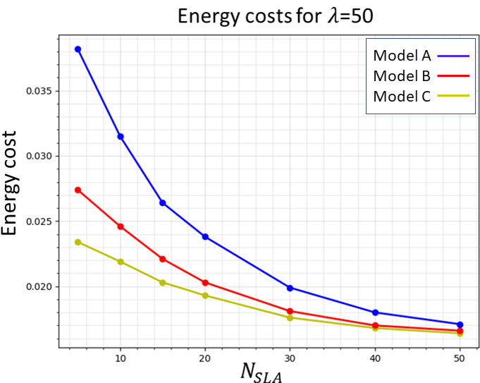
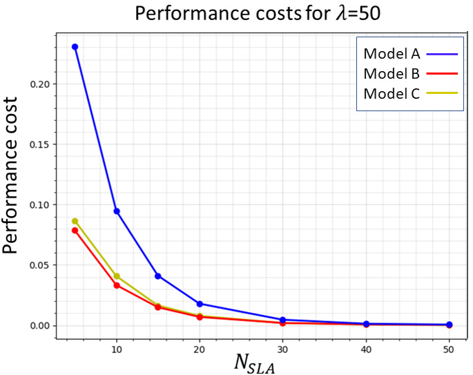
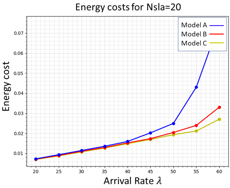
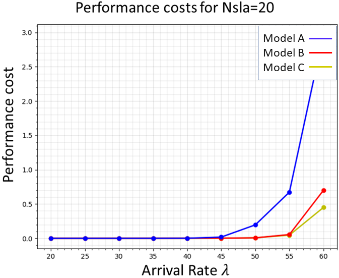
Figure 3: Energy and performance costs given fixed SLA or arrival rate

8 Conclusions and further work

In this paper we have compared theoretically and numerically two different approaches to minimise the global cost integrating both performance and energy consumption in an auto scaling cloud system. The relevance of this study for a cloud provider is to provide an auto scaling policy very quickly to minimise its financial cost (around $38$ seconds for $128$ VMs and $800$ customers). We exhibit that the best static heuristics are strongly outperformed by SMDP models and that hysteresis presents a significant improvement. Our next steps will be to enlarge the model by including more general arrival process as burst traffic predicted from a measurement tool and second to build a cloud prototype to evaluate the performances of our policies in a real environment.

Appendix A Resources management examples

We detail now the management resources.

Example 2.

We display an example for all cases according to Definition 7, to illustrate the difference of optimal solutions between both approaches. Solutions returned by MDP algorithms are displayed without the shift operation. We take the following costs values $C_{a}=C_{d}=2,~{}C_{h}=C_{s}=5,~{}C_{r}=10$ with $K=16,~{}B=100$ scenario.

Medium arrival case

Consider the following queueing parameters: $\lambda=500$, $\mu=100$.

The MDP algorithm provides the following solution: $C^{*}=25,239\mbox{; and}$

$L^{*}=[2,4,5,7,8,10,11,13,15,16,18,19,21,23,24];$

$l^{*}=[0,1,3,4,5,6,7,8,9,10,11,12,13,14,15].$

The heuristic in the (MC) model provides the following solution: $C^{*}=25,239\mbox{; and :}$

$F^{*}=[1,3,4,6,7,9,10,12,14,15,17,18,20,22,23];$

$R^{*}=[1,2,4,5,6,7,8,9,10,11,12,13,14,15,16].$

We can observe here that the two solutions are identical since (MDP) algorithm finds thresholds in all levels.

Low arrival case

Consider the following queueing parameters: $\lambda=50$, $\mu=100$.

The MDP algorithm provides the following solution: $C^{*}=9,99323\mbox{; and :}$

$L^{*}=[12,26,39,52,64,77,90,\infty,\infty,\infty,\infty,\infty,\infty,\infty,\infty];$

$l^{*}=[0,1,2,3,4,5,6,7,8,9,10,11,12,13,14].$

The heuristic in the (MC) model provides the following solution: $C^{*}=9,99375\mbox{; and :}$

$F^{*}=[11,25,28,39,51,58,70,72,88,94,95,96,97,98,99];$

$R^{*}=[1,2,3,4,5,6,7,8,9,10,11,12,13,14,15].$

Since the load in the system is very low, the (MDP) algorithm does not need to turn ON all virtual resources. However, we observe that (MC) approach still activate all levels but tries to activate as late as possible to compensate that it does not need to turn ON more virtual resources. It induces a small supplementary costs since these activations will ’never’ happen in this system.

High arrival case

Consider the following queueing parameters: $\lambda=1000$, $\mu=100$.

The MDP algorithm provides the following solution: $C^{*}=119,756\mbox{; and :}$

$L^{*}=[2,3,4,5,6,7,9,10,11,13,16,24,56,69,82];$

$l^{*}=[0,0,0,\ldots,0,0,0,10,12,14].$

The heuristic in the (MC) model provides the following solution: $C^{*}=220,879\mbox{; and :}$

$F^{*}=[2,4,6,8,11,13,16,21,27,37,48,61,75,88,96];$

$R^{*}=[1,2,3,4,5,6,7,8,11,16,22,26,29,30,34].$

We can observe here that (MC) approach still define deactivation thresholds in any levels (due to its model and isotone hysteresis constraints) leading to a higher mean cost.

Appendix B Complements on SMDP anaysis

. We give now some examples to illustrate the theoretical analysis of the SMDP.

B.1 Multichain MDP example

Example 3.

We show a scenario where the MDP policy $q$ will generate a multichain Markov chain where we can observe several recurrent classes. This example is represented on Figure 4.

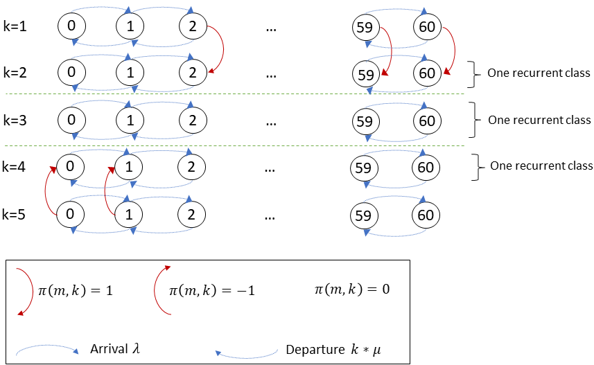
Figure 4: Example of an isotone hysteresis multichain MDP

B.2 Temporal behaviour of two approaches

We display two figures showing the different temporal behaviour between the two approaches: Markov chain and MDP. The first figure (Figure 5) explains the temporal transition in the Markov chain approach while the second figure (Figure 6) explains the temporal transition for MDP.

Figure 5: Behaviour of the agent in the Markov chain Model

Figure 6: Behaviour of the agent in the MDP Model

B.3 Transformation of MDP policy into a threshold policy

We display an example of generated Markov chain by a policy $q$ of the MDP agent. We show in this figure how we can transform the MDP policy into a threshold policy.

Example 4.

Example of the transformation of a MDP policy into a threshold policy with 3 virtual machines. This case is illustrated on Figure 7.

Figure 7: Example of the threshold policy transformation in a low scale scenario

The optimal threshold vector in this example would be: $L^{*}=[3,4]\mbox{ and }l^{*}=[0,1]$

Appendix C Experimental results for concrete scenarios

We display several supplementary experimental (Section 7.3) results for concrete scenarios by comparing the behaviour of first activation thresholds and global costs when we take different parameterisation of the system (arrival rate $\lambda$, SLA metric $N_{sla}$). These are given in the figures later. Figure 8 represents the mean global cost while Figure 9 gives the evolution of the first threshold.

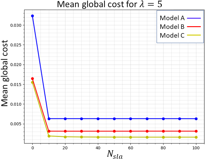
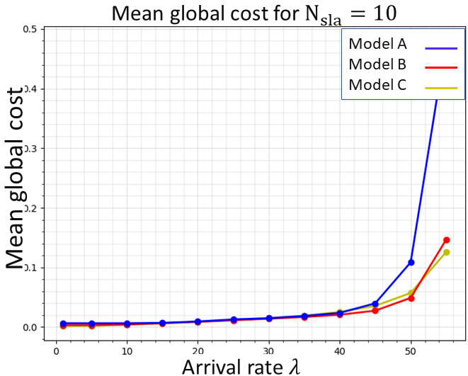
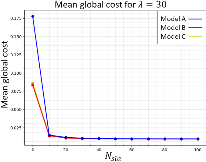
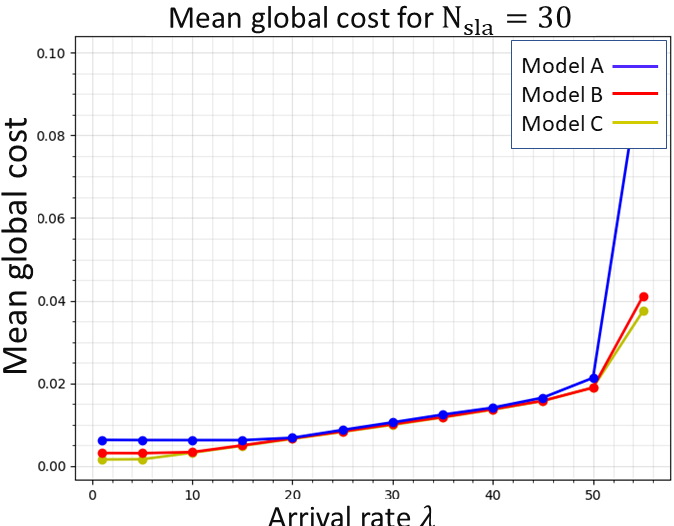
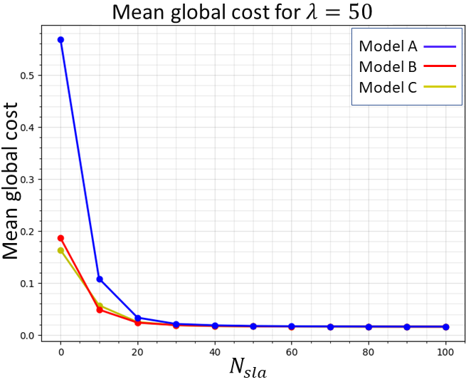
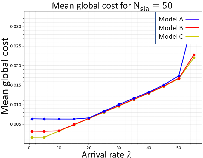
Figure 8: Mean global cost for the three models given a fixed Nsla or a fixed lambda

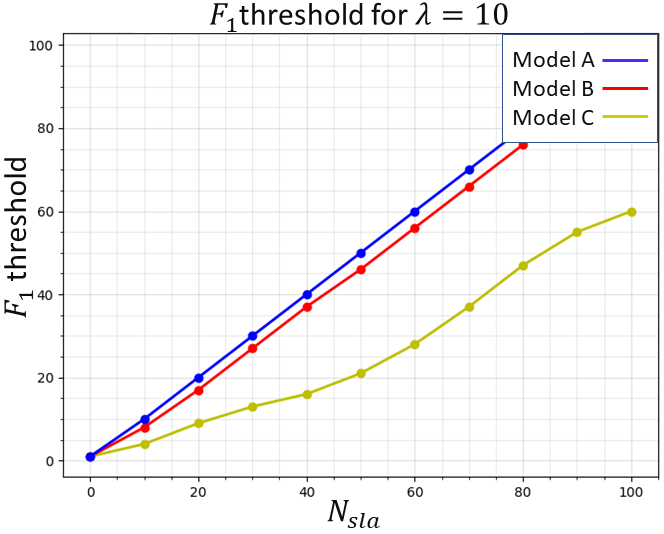
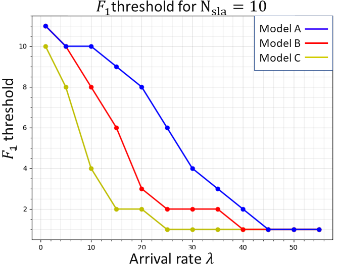
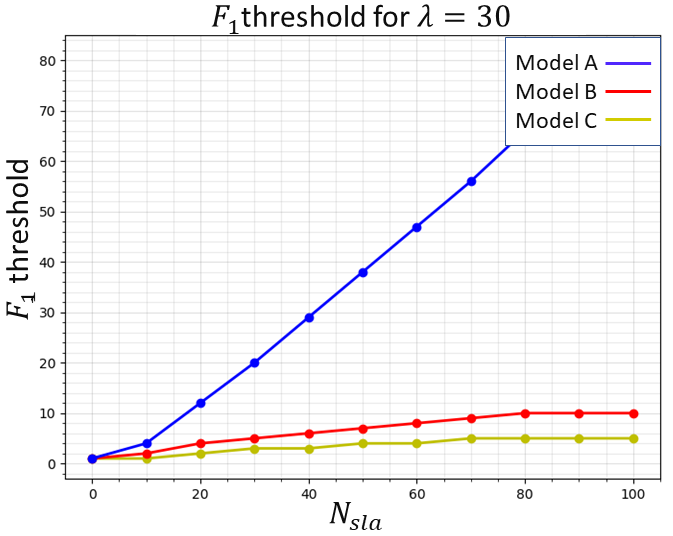
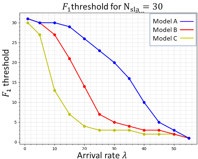
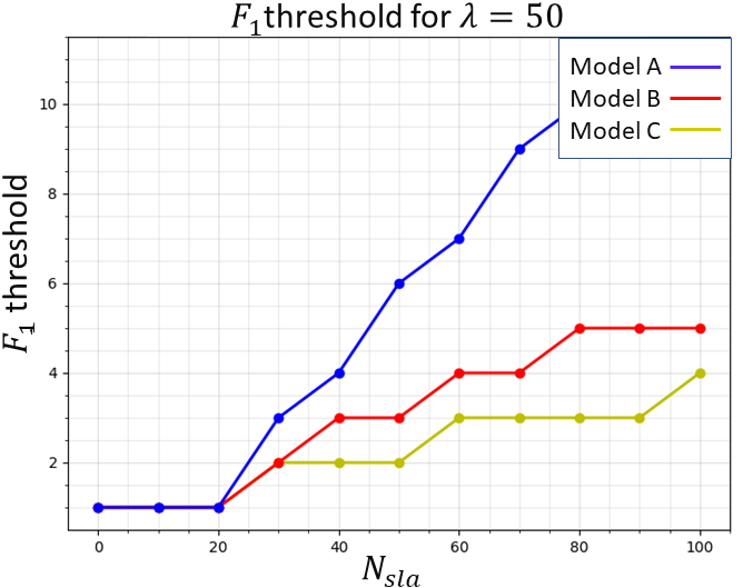
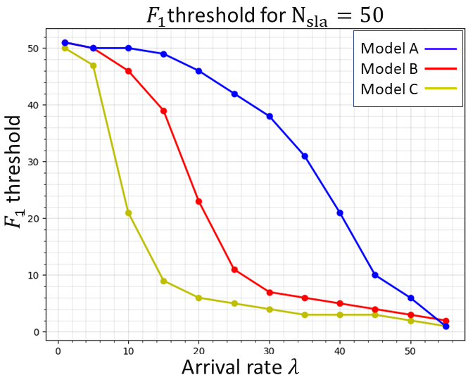
Figure 9: F1 thresholds for the three models given a fixed Nsla or a fix lambda

Appendix D Pseudo-Codes of algorithms

We present the pseudo-codes of heuristics described in section 4.3. To describe the different algorithms, we define the following notations:

- solve$[F,R]$: function that, for a given vector of thresholds, generates its associated Markov chain, computes its stationary distribution with the aggregation method then computes the mean cost $\overline{C}_{[F,R]}^{\pi}$ .

- $C^{*}$: the solution of the optimisation problem and $[F,R]^{*}$ the optimal vector of thresholds.

1

Input: $\lambda,\mu,B,K,C_{a},C_{d},C_{h},C_{s},C_{r}$, the cloud system parameters

Output: $[F,R]^{*},C^{*}$

2 Initialise a vector of thresholds $[F,R]_{0}$

3Apply solve$[F,R]$ for the current vector

4while improvement=TRUE do

       /* Activation Thresholds */

5      

6      for $k\in[1,K-1]$ do

7             for $F_{k}$ respecting constraints do

8                   solve$[F,R]$ and store the vector if improvement

9            

10      

11      

      /* Deactivation Thresholds */

12      

13      for $k\in[1,K-1]$ do

14             for $R_{k}$ respecting constraints do

15                   solve$[F,R]$ and store the vector if improvement

16            

17      

Algorithm 1 Best per level

1

Input: $\lambda,\mu,B,K,C_{a},C_{d},C_{h},C_{s},C_{r}$, the cloud system parameters

Output: $[F,R]^{*},C^{*}$

2 Initialise a vector of thresholds $[F,R]_{0}$

3Apply solve$[F,R]$ for the current vector

4while improvement=TRUE do

       /* We generate $\mathbf{V}$ by giving +1 or -1 to each elements of the vector, $\text{card}(\mathbf{V})=4(K-1)$ */

5       Generate the neighbourhood $\mathbf{V}$ of $[F,R]$

6      for $[F,R]\in\mathbf{V}$ do

7             solve$[F,R]$ and store the vector if improvement

8      

Algorithm 2 Neighbourhood local search

1

Input: $\lambda,\mu,B,K,C_{a},C_{d},C_{h},C_{s},C_{r}$, the cloud system parameters

Output: $[F,R]^{*},C^{*}$

2 Initialise a vector of thresholds $[F,R]_{0}$

3Apply solve$[F,R]$ for the current vector

4while improvement=TRUE do

       /* Activation Threshold 1st Level */

5      

6      First level k=1

7      for $m\in[1,B]$ do

8             Compute $\phi^{A}_{1}(m)$

9            When $\phi^{A}_{1}(m)$ > 0 ,BREAK, then $F_{1}$ = m if constraints respected

10      

      /* Activation thresholds level k */

11      

12      for $k\in[2,K-1]$ do

13             for $m\in[F_{k-1}+1,B]$ do

14                   Compute $\phi^{A}_{k}(m)$

15                  When $\phi^{A}_{k}(m)$ > 0 ,BREAK, then $F_{k}$ = m if constraints respected

16            

17      

      /* Deactivation Threshold 1st Level */

18      

19      First level k=1

20      for $m\in[0,F_{k}-1]$ do

21             Compute $\phi^{D}_{1}(m)$

22            When $\phi^{D}_{1}(m)\geq 0$ ,BREAK, then $R_{1}$ = m if constraints respected

23      

      /* Deactivation thresholds level k */

24      

25      for $k\in[2,K]$ do

26             for $m\in[R_{k-1}+1,F_{k}-1]$ do

27                   Compute $\phi^{D}_{k}(m)$

28                  When $\phi^{D}_{k}(m)\geq 0$ ,BREAK, then $R_{k}$ = m if constraints respected

29            

30      

Algorithm 3 M/M/K/B approximation

References

- [1] Observatoire de l’industrie Electrique. Le cloud, les data centers et l’énergie, January 2017.
- [2] T. Mastelic and I. Brandic. Recent trends in energy-efficient cloud computing. IEEE Cloud Computing, 2:40–47, 2015.
- [3] T. Lorido-Botran, J. Miguel-Alonso, and J.A. Lozano. A review of auto-scaling techniques for elastic applications in cloud environments. J. Grid Computing, 12:559–592, 2014.
- [4] A. Benoit, L. Lefèvre, A.-C. Orgerie, and I. Rais. Reducing the energy consumption of large scale computing systems through combined shutdown policies with multiple constraints. Int. J. High Perform. Comput. Appl., 32(1):176–188, 2018.
- [5] N.M. Asghari, M. Mandjes, and A. Walid. Energy-efficient scheduling in multi-core servers. Computer Networks, 59:33–43, 2014.
- [6] M.Y. Kitaev and R.F. Serfozo. M/M/1 queues with switching costs and hysteretic optimal control. Operations Research, 47:310–312, 1999.
- [7] J. C. S. Lui and L. Golubchik. Stochastic complement analysis of multi-server threshold queues with hysteresis. Performance Evaluation, 35:19–48, 1999.
- [8] S. Shorgin, A. Pechinkin, K. Samouylov, Y. Gaidamaka, I. Gudkova, and E. Sopin. Threshold-based queuing system for performance analysis of cloud computing system with dynamic scaling. In AIP Conference, volume 1648, 2015.
- [9] T. Tournaire, H. Castel, E. Hyon, and T. Hoche. Generating optimal thresholds in a hysteresis queue: a cloud application. In IEEE Mascots, pages 283–294, 2019.
- [10] Amazon. AWS Auto Scaling, 2018.
- [11] D.P. Warsing, W. Wangwatcharakul, and R.E. King. Computing optimal base-stock levels for an inventory system with imperfect supply. Computers and Operations Research, 40:2786–2800, 2013.
- [12] D.-P. Song. Optimal Control and Optimization of Stochastic Supply Chain Systems. Springer-Verlag, 2013.
- [13] M. Kurpicz, A.-C. Orgerie, and A. Sobe. How much does a VM cost? energy-proportional accounting in VM-based environments. In PDP, pages 651–658, 2016.
- [14] J. Krzywda, A. Ali-Eldin, T.E. Carlson, P.-O. Ostberg, and E. Elmroth. Power-performance tradeoffs in data center servers: DVFS, CPU pinning, horizontal and vertical scaling. Future Generation Computer Systems, pages 114–128, 2018.
- [15] I.J.B.F. Adan, V.G. Kulkarni, and A.C.C. van Wijk. Optimal control of a server farm. INFOR: Information Systems and Operational Research, 51(4):241–252, 2013.
- [16] A. Gandi, M. Harchol-Balter, and I. Adan. Server farms with setup costs. Performance Evaluation, 67(11):1123–1138, 2010.
- [17] I. Mitrani. Managing performance and power consumption in a server farm. Annals of Operations Research, 202:121–134, 2013.
- [18] J. R. Artalejo, A. Economou, and M. J. Lopez-Herrero. Analysis of a multiserver queue with setup times. Queueing Systems, 51(1-2):53–76, 2005.
- [19] D. Ardagna, G. Casale, M. Ciavotta, J.F. Pérez, and W. Wang. Quality-of-service in cloud computing: modeling techniques and their applications. JISA, 5, 2014.
- [20] J. Teghem. Control of the service process in a queueing system. EJOR, 23(2):141–158, 1986.
- [21] Z. Yang, M.-H. Chen, Z. Niu, and D. Huang. An optimal hysteretic control policy for energy saving in cloud computing. In GLOBECOM, pages 1–5, 2011.
- [22] N. Lee and V. G. Kulkarni. Optimal arrival rate and service rate control of multi-server queues. Queueing Syst. Theory Appl., 76(1):37–50, 2014.
- [23] D.S. Szarkowicz and T.W. Knowles. Optimal control of an M/M/S queueing system. Operations Research, 33(3):644–660, 1985.
- [24] S.K. Hipp and U.D. Holzbaur. Decision processes with monotone hysteretic policies. Operations Research, 36(4):585–588, 1988.
- [25] J. Niño-Mora. Resource allocation and routing in parallel multi-server queues with abandonments for cloud profit maximization. Computers and Operations Research, 103:221–236, 2019.
- [26] A.C. Randa, M.K. Dogru, C. Iyigun, and U. Özen. Heuristic methods for the capacitated stochastic lot-sizing problem under the static-dynamic uncertainty strategy. Computers and Operations Research, 109:89–101, 2019.
- [27] A.A. Kranenburg and G.J. van Houtum. Cost optimization in the (S-1, S) lost sales inventory model with multiple demand classes. Oper. Res. Lett., 35(4):493–502, 2007.
- [28] M. Braglia, D. Castellano, L. Marrazzini, and D. Song. A continuous review, (Q, r) inventory model for a deteriorating item with random demand and positive lead time. Computers and Operations Research, 109:102–121, 2019.
- [29] C.-H. Wu, W.-C. Lee, J.-C. Ke, and T-H. Liu. Optimization analysis of an unreliable multi-server queue with a controllable repair policy. Computers and Operations Research, 49:83–96, 2014.
- [30] O.C. Ibe and J. Keilson. Multi-server threshold queues with hysteresis. Performance Evaluation, 21:185–213, 1995.
- [31] M.M. Kandi, F. Aït-Salaht, H. Castel-Taleb, and E. Hyon. Analysis of performance and energy consumption in the cloud. In EPEW, pages 199–213, 2017.
- [32] M.L. Puterman. Markov Decision Processes: Discrete Stochastic Dynamic Programming. Wiley, 1994.
- [33] A. Jean-Marie. marmoteCore: a Markov modeling platform. In VALUETOOLS, pages 60–65, 2017.
- [34] Amazon. Amazon EC2 pricing, 2019.
- [35] D. Guyon, A-C. Orgerie, C. Morin, and D. Agarwal. Involving users in energy conservation: A case study in scientific clouds. International Journal of Grid and Utility Computing, 2018.