RSSI-Based Location Classification Using
a Particle Filter to Fuse Sensor Estimates

Abstract

For Cyber-Physical Production Systems (CPPS), localization is becoming increasingly important as wireless and mobile devices are considered an integral part. While localizing targets in a wireless communication system based on the Received Signal Strength Indicator (RSSI) of transmitted beacons is a well-known strategy, it is often limited by the quality of the RSSI sensors We propose to use a particle filter that fuses RSSI measurements of different sensors. This allows us to incorporate sensor non-idealities in our model, and achieve a high-quality position estimate that is not limited by them. The estimation performance is evaluated using real-world measurements of a car in a chamber. In the second step, we use Machine Learning (ML) to classify where the vehicle is. Our results show that the location output of the particle filter is a better input to the ML technique than the raw RSSI data, and we achieve improved classification accuracy while simultaneously reducing the number of features that the ML has to consider. We furthermore compare the performance of multiple ML algorithms and demonstrate that SVMs provide the overall best performance for the given task.

I Introduction

In Cyber-Physical Production Systems (CPPS), knowing the location of moving objects, be it robots or vehicles, is already often essential, and with the advent of cyber-physical systems and smart agents, this issue is expected to become even more pressing [1]. Therefore, a significant effort is being put into the ability to localize objects in such a setting. Broadly speaking, there are systems specifically designed for this task, and systems where the localization is done as a side benefit of another system. Dedicated systems include radar [2], as well as Global Navigation Satellite System (GNSS) systems. While the former require a distributed net of radar sensors, the latter pose large challenges when deployed indoor [3, 4].

Alternatively, existing systems are exploited. There, the most obvious choices are visual tracking through the use of camera systems, and exploiting radio communications that are deployed in the tracked object. Using video systems for tracking is currently of high interest within the machine and deep learning community [5, 6]. A major downside of the visual approach is that the camera system must be adapted to cover the relevant area, and a traceable object does nothing to initiate being tracked. On the other hand, RF-based localization works based on beacons transmitted from a traceable object and is therefore harder to miss. Estimation of location based on the Received Signal Strength Indicator (RSSI) has been studied for some time [7, 8, 9]. The RSSI based estimation usually resorts to variants of triangulation or multilateration [10]. However, due to the often limited dynamic range of RSSI estimates, and the noise floor of receivers, multilateration may not be a solution, and authors rarely apply more advanced schemes such as maximum likelihood estimation [11].

I-A Contribution

We present an approach that allows us to localize a target transmitting a Bluetooth beacon using distributed low-cost sensors with limited dynamic range and high noise floor. Similar to the idea sketched but not implemented in [12], we employ a sensor fusion particle filter [13] to convert a large number of low-quality sensor measurements into one high-quality position and velocity estimate. We also account for the sensor placement on a vehicle resulting in a non-omnidirectional antenna pattern. Our results, which are based on real-world measurements, show that this choice allows accurately fusing the highly imperfect sensor data. This is presented in Section III.

We then use the high-quality position estimates to classify three states that are especially relevant to us, by using Machine Learning (ML) techniques. We compare three different classifiers, Support Vector Machine (SVM), K Nearest Neighbors (KNN) and Random Forest (RF) on the location estimates. Furthermore, we analyse the influence of data-prescaling. This two-step process improves the classification accuracy while simultaneously reducing the number of required features for the Machine learning model. The results are shown in Section IV.

I-B Notation

Scalars are written as $x$, while vectors and matrices are denoted as lower- and uppercase boldface respectively (e.g. ${\mathbf{x}}$ and $\mathbf{X}$). Time indices are indicated using square brackets. The Euclidean norm is written as $\|\cdot\|$. $x[t]$ denotes the sample of $x$ at discrete-time index $t$.

II System Model

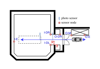
Figure 1: Measurement Setup. When the car is fully to the left of the left photo sensor, we assign state 2. If it is completely right of the right photo sensor, we assign state 0. Otherwise, we assign state 1.

We base our analysis on real-world measurements taken from the SAL Autarkic Localization RSSI BLE Dataset (SAL-RB-Dataset) [14]. This data set presents the scenario as given in Fig. 1. A car moves in and out of a chamber along the $x$-axis, where the positive direction points outwards of the chamber. From the data set’s provided photo sensor data, we compute labels for three distinct states: the car being outside of the chamber (right of the rightmost photo sensor) is designated state $0$, the car being inside the chamber in the end position fully past the left photo sensor is state $2$, and the transition region where the car has entered the chamber but not yet reached the defined position is designated state $1$. The car transmits periodically at an interval of $\Delta t=100$ ms using the Energy and Power Efficient Synchronous Sensor Network (EPhESOS) protocol and the Bluetooth Low Energy (BLE) physical layer [15]. This Time Division Multiple Access (TDMA) protocol allows exact time synchronization of the measurement series. At six positions, sensors are placed that record the RSSI of the transmitted Bluetooth beacons. These sensors are low-cost in nature, and therefore have a very limited dynamic range and Signal-to-Noise Ratio (SNR).

We use six sets of measurements, that all reflect the described scenario. Each measurement contains between two and five drives in and out of the chamber. Figure 2 shows the RSSI data in dBm of one such measurement. We refer to the three-dimensional position and velocity of the car as $\mathbf{p}$ and $\mathbf{v}$. In our setup, the car moves purely along the $x$-axis. Hence, we introduce the vector ${\mathbf{x}}$ describing the cars state, which is comprised of the current position and velocity along the $x$-axis

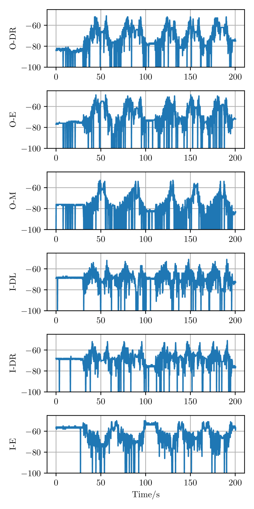
Figure 2: Exemplary RSSI measurements in dBm of the $6$ used sensors.

$${\mathbf{x}}=\begin{bmatrix}p^{x}\\ v^{x}\end{bmatrix}\,.$$ (1)

While the car will accelerate and decelerate at the ends of the movement regions, we assume that a uniform movement model holds for the majority of the time

$${\mathbf{x}}[t+1]=\underbrace{\begin{bmatrix}1&1\\ 0&1\end{bmatrix}}_{{\mathbf{A}}}{\mathbf{x}}[t]\,.$$ (2)

Given the positions of the transmitter ${\mathbf{p}}$ and the $s$ th sensor $\mathbf{q}_{s}$, the signal power at the sensor is provided in dB by the pathloss equation

$$l({\mathbf{p}},\mathbf{q}_{s})= P_{\text{tx}}-{PL}_{0}$$

$$-n10\log_{10}\left(\frac{\|\mathbf{q}_{s}-{\mathbf{p}}\|}{1\,\text{m}}\right)+\pi({\mathbf{p}},\mathbf{q}_{s})\,,$$ (3)

where $\text{PL}_{0}$ is the pathloss at $1$ m, $n$ is the pathloss exponent, and $\pi({\mathbf{p}},\mathbf{q}_{s})$ represents the antenna pattern of the transmitter. Since the transmitter is mounted on the front side of a car, we expect significant directionality, even if the mounted antenna is originally omnidirectional. The RSSI estimate at the receiving sensor nodes is calculated in dB, and due to the low-cost nature, significantly noisy. Furthermore, we assume that below a threshold $P_{\text{floor}}$, the sensor does not capture the pathloss anymore, and instead reports a noisy realization of the noise floor. Hence, we assume that the actual likelihood function for a given RSSI measurement $P_{\text{rx}}$ in dB is normal distributed

$$f(P_{\text{rx}}|{\mathbf{p}},\mathbf{q}_{s})= \frac{1}{\sqrt{2\pi\sigma^{2}}}\exp\left(-\frac{(P_{\text{rx}}-\mu_{P})^{2}}{2\sigma^{2}}\right)\,,$$

$$\mu_{P}= \max\big{(}P_{\text{floor}},l({\mathbf{p}},\mathbf{q}_{s})\big{)}\,.$$ (4)

As $p^{y}$ and $p^{z}$ are constant throughout the measurement, only the $p^{x}$ coordinate is required, and $f(P_{\text{rx}}|{\mathbf{p}},\mathbf{q}_{s})=f(P_{\text{rx}}|{\mathbf{x}},\mathbf{q}_{s})$.

III Localization via Sensor Fusion Particle Filtering

In this section, we estimate the car position from the low-quality RSSI recordings of the sensors. The particle filter, as well as the sensor fusion, is taken from [16]. Fundamentally, the filter is initialized once, and then the steps prediction, update, and resampling are cyclically executed. To initialize, we use $n=300$ particles that have the shape given in Eq. 1.

Initialization

We draw $n$ $p^{x}$ from a uniform distribution $\mathcal{U}(-25,25)$, and $v^{x}$ from $\mathcal{U}(-3,3)$. Each particle is associated with a weight $w_{i}$ with $i\in\mathbb{N}$ and $i\in[1,n]$ that is initially set to $w_{i}=n^{-1}$.

Predition

For every particle ${\mathbf{p}}_{i}$, we compute the prediction

$${\mathbf{x}}_{i}[t+1]={\mathbf{A}}{\mathbf{x}}_{i}[t]+{\mathbf{n}}[t]\,.$$ (5)

${\mathbf{n}}[t]$ is a multivariate normal driving noise term that is zero-mean with a covariance matrix

$$\mathbf{C}=\begin{bmatrix}4&0\\ 0&4\end{bmatrix}\,.$$ (6)

Update

Now, we update the estimates based on the recorded measurements. For every sensor $s$, an RSSI value $P_{s}[t]$ is recorded, unless the sensor refuses to provide a measurement at that point. We then calculate the local likelihood function from sensor $s$ to particle $p_{i}$ as the conditional probability density $f_{s}^{(i)}(P_{s}[t]|{\mathbf{x}}_{i},\mathbf{q}_{s})$. If a sensor does not provide a measurement, this term will be set to $1$. Then, the sensor fusion is performed by updating the weights for the particles according to

$$w_{i}^{\prime}= \prod_{s\in\mathcal{S}}f_{s}^{(i)}(P_{s}[t]|{\mathbf{x}}_{i},\mathbf{q}_{s})\,,$$

$$w_{i}= \frac{w_{i}^{\prime}}{\sum_{j}w_{j}^{\prime}}\,,$$ (7)

where $\mathcal{S}$ is the set of all existing sensors. Now an estimate of the target, as well as the estimation variance is computed as

$$\hat{{\mathbf{x}}}= \sum_{i}w_{i}{\mathbf{x}}_{i}\,,$$

$$\hat{\mathbf{\sigma}}^{2}= \sum_{i}w_{i}({\mathbf{x}}_{i}-\hat{{\mathbf{x}}})^{2}\,.$$ (8)

Resampling

To improve the estimation quality, a new set of $n$ particles is resampled from the old set with replacements with the probability of drawing ${\mathbf{p}}_{i}$ being $w_{i}$. Afterwards, the weights are reset to $w_{i}=n^{-1}$, and the next iteration starts at prediction.

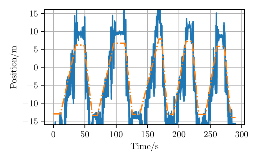
(a) Omnidirectional estimation.

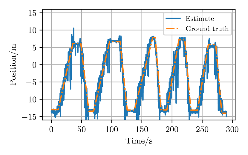
(b) Directional estimation using Eq. 10.

Figure 3: Performance of the position estimation compared to the ground truth. (a) shows the filter with an omnidirectional pattern, while (b) uses the antenna model from Eq. 10.

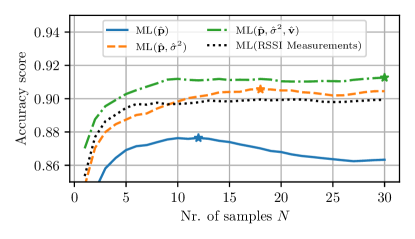
(a) SVM, Standard Scaler

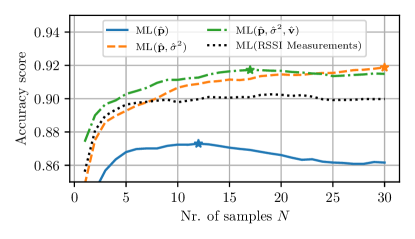
(b) SVM, Power Transformer

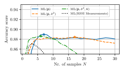
(c) KNN, Standard Scaler

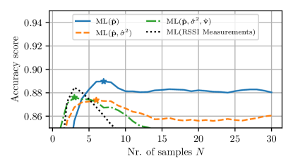
(d) KNN, Power Transformer

(e) RF, Standard Scaler

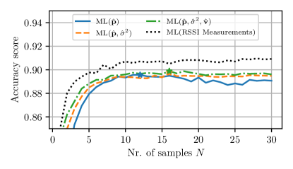
(f) RF, Power Transformer

Figure 4: Accuracy scores of the ML classified estimates. Note the scaling of the $y$-axis. Locations of maxima are denoted with stars.

The pathloss model as given in Eq. 3 contains the term $P_{tx}-PL_{0}$, which, excluding the antenna pattern, refers to the expected received power at $1$ m distance. As the cars closest position to all sensors has distances of roughly $1$ m, we set this term in the likelihood function to the maximum measured RSSI value of a given sensor. The pathloss exponent is set to $n=2$, reflecting the strong line-of-sight components that we expect. The variance of the likelihood function is set to $\sigma^{2}=9$.

The gain of the antenna pattern is given as

$$\pi(\mathbf{p},\mathbf{q})=\left\{\begin{array}[]{rrcl}0\,\text{dB},&0\leq&|\alpha|&<\frac{\pi}{3}\\ -6\,\text{dB},&\frac{\pi}{3}\leq&|\alpha|&<\frac{3\pi}{4}\\ -10\,\text{dB},&\frac{3\pi}{4}\leq&|\alpha|&<\pi\end{array}\right.,$$ (9)

with the angle calculated as

$$\alpha=\cos^{-1}\left(\frac{p^{x}-q^{x}}{\|\mathbf{p}-\mathbf{q}\|}\right)\,.$$ (10)

These assumptions are kept simple on purpose, in the hope that the sensor fusion allows to correct slight inaccuracies. Figure 3 demonstrates the output of the location estimation for one given measurement. The ground truth is computed from the sensor information and cameras. Figure 3a shows the performance with an omnidirectional assumption, which fails to estimate the off-center positions well. Figure 3b illustrates that the directional antenna pattern is effective at correcting for these errors.

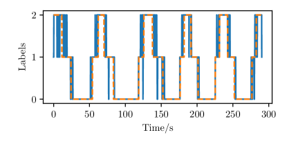
(a) SVM, Standard Scaler, N=3

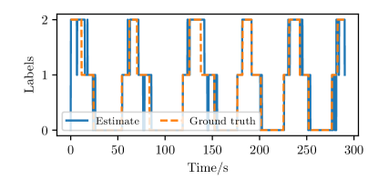
(b) SVM, Standard Scaler, N=16

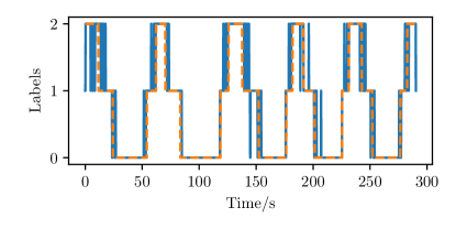
(c) SVM, Power Transformer, N=3

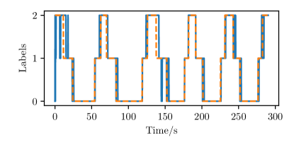
(d) SVM, Power Transformer, N=16

Figure 5: Example output of SVM($\hat{\mathbf{p}},\hat{\mathbf{\sigma}}^{2},\hat{\mathbf{v}}$) for different memory lengths, and scalers.

IV ML-Based Position Detection

IV-A Machine Learning Setup

TABLE I: Classifiers with parameters

Estimator	Parameters
Random Forest	n_estimators=100, criterion=”gini”
K Nearest Neighbors	n_neighbors=5
SVM	kernel=”rbf”

Based on the position and velocity estimates of the particle filter, we conduct the classification of three states as described in Section II. To this end, we employ purposefully simple ML techniques. We consider three typical algorithms, namely KNN, a RF, and a SVM. The specific parameters of the ML classifiers in the used library Scikit-learn[17] are given in Table I. We combine these with three choices of data scalers, the standard scaler, the robust scaler, and the power transformer. As feature vectors, we consider the position and velocity estimates $\hat{\mathbf{p}}$ and $\hat{\mathbf{v}}$ derived from $\hat{\mathbf{x}}$, as well as the variance estimate of the position estimate $\hat{{\sigma}}^{2}_{p}$. Additionally, to enhance the estimation, we consider a short-term history of the features. We do this by constructing a Toeplitz-matrix of width $N$ out of each feature vector, and use the columns of the matrices as individual feature vectors.

TABLE II: Accuracy Scores.

Model	Scaler	$\mu^{x}$	$\mu^{x},\sigma^{x}$	$\mu^{x},\sigma^{x},\mu^{v}$
SVM	Standard Scaler	0.8764	0.9056	0.9126
	Robust Scaler	0.8764	0.8971	0.9051
	Power Transformer	0.873	0.9188	0.9172
KNN	Standard Scaler	0.8896	0.8843	0.8862
	Robust Scaler	0.8896	0.8586	0.8483
	Power Transformer	0.8897	0.8738	0.876
RF	Standard Scaler	0.8953	0.8963	0.9
	Robust Scaler	0.8944	0.8967	0.8987
	Power Transformer	0.8957	0.8975	0.8989

For the evaluation, we draw all possible combinations of three of the six data sets to train the ML classifiers. Afterwards, we validate the fits against all remaining three data sets individually and compute the accuracy score defined as the fraction of correctly identified labels over the number of all instances. We don’t split and shuffle the measurement runs, but instead use them as a whole either in training or testing. This approach avoids overfitting dominant measurement runs.

IV-B Results

Figure 4 shows the performance of the ML classifiers for different parameter combinations, and different classifier-scaler combinations. The different curves show ML classifiers based on either the position estimate, the position and corresponding variance estimate, or position, velocity, and variance estimates. $N$ denotes the memory size, which is the number of samples that are considered per feature. Additionally, the plot depicts the results of the corresponding ML classifier using the raw sensor values without the particle filter preprocessing. Similarly, Table II shows the accuracy scores for each combination of input features, scaler and model if the optimum memory depth is chosen. As the table shows, the robust scaler uniformly performs worst, hence it has been ommited in Figure 4. Furthermore, for our application, the SVM proves to perform uniformly better than the RF, while KNN performs by far the worst. Among the SVM classifiers using only the position estimate results in an overall bad behaviour. However, by adding at least the variance estimate, or even better, both variance and velocity estimate, the estimator drastically improves. The main reason for this difference is the transition region in the door. Here, the position estimate can be relatively uncertain, and will lead to many misclassifications. On the other hand, by including variance and velocity estimates, this estimate becomes much more robust. We furthermore see that in our case, the power transforming prescaler provides the overall best performance, and gains $0.5\,\%$ accuracy compared to the standard scaler.

Figure 5 illustrates the classification quality of this classifier with memory depths of three and $16$, against the reference labels. Here, we see the discussed effect, that the transitioning label $1$ proves to be the most challenging. Both standard and power scaler show strong oscillations in the transition regions when using a memory length of $N=3$. When increasing the memory length to $16$, it is those regions that see the most improvement.

V Conclusions

Using a particle filter as an intermediate step before machine learning allows fusing multiple low-quality feature sources into a high-quality feature source. Our results show that deriving location, and velocity mean and variance estimates and using them as features improves the performance of many ML classifiers, while simultaneously reducing the number of input features of the classifier. In our scenario, the best results were achieved using a SVM classifier with a power transforming prescaler.

The provided results, based on real-world measurements, prove the viability of such hybrid approaches. Additionally, doing the sensor fusion before the classification opens up the possibility of rearranging the sensor setup, and adapting the fusion process, while leaving the trained classification unchanged.

References

- [1] Paulo Leitão, Stamatis Karnouskos, Luis Ribeiro, Jay Lee, Thomas Strasser, and Armando W. Colombo, “Smart Agents in Industrial Cyber–Physical Systems,” Proceedings of the IEEE, vol. 104, no. 5, pp. 1086–1101, May 2016.
- [2] Randolf Ebelt, Amin Hamidian, Denys Shmakov, Tao Zhang, Viswanathan Subramanian, Georg Boeck, and Martin Vossiek, “Cooperative Indoor Localization Using 24-GHz CMOS Radar Transceivers,” IEEE Transactions on Microwave Theory and Techniques, vol. 62, no. 9, pp. 2193–2203, Sept. 2014.
- [3] Shahriar Nirjon, Jie Liu, Gerald DeJean, Bodhi Priyantha, Yuzhe Jin, and Ted Hart, “COIN-GPS: Indoor localization from direct GPS receiving,” in Proceedings of the 12th Annual International Conference on Mobile Systems, Applications, and Services, New York, NY, USA, June 2014, MobiSys ’14, pp. 301–314, Association for Computing Machinery.
- [4] Ali Yassin, Youssef Nasser, Mariette Awad, Ahmed Al-Dubai, Ran Liu, Chau Yuen, Ronald Raulefs, and Elias Aboutanios, “Recent Advances in Indoor Localization: A Survey on Theoretical Approaches and Applications,” IEEE Communications Surveys Tutorials, vol. 19, no. 2, pp. 1327–1346, Secondquarter 2017.
- [5] Gioele Ciaparrone, Francisco Luque Sánchez, Siham Tabik, Luigi Troiano, Roberto Tagliaferri, and Francisco Herrera, “Deep learning in video multi-object tracking: A survey,” Neurocomputing, vol. 381, pp. 61–88, Mar. 2020.
- [6] Yingkun Xu, Xiaolong Zhou, Shengyong Chen, and Fenfen Li, “Deep learning for multiple object tracking: A survey,” IET Computer Vision, vol. 13, no. 4, pp. 355–368, Jan. 2019.
- [7] Yixin Wang, Qiang Ye, Jie Cheng, and Lei Wang, “RSSI-Based Bluetooth Indoor Localization,” in 2015 11th International Conference on Mobile Ad-Hoc and Sensor Networks (MSN), Dec. 2015, pp. 165–171.
- [8] Hetal P. Mistry and Nital H. Mistry, “RSSI Based Localization Scheme in Wireless Sensor Networks: A Survey,” in 2015 Fifth International Conference on Advanced Computing Communication Technologies, Feb. 2015, pp. 647–652.
- [9] Forough Yaghoubi, Ali-Azam Abbasfar, and Behrouz Maham, “Energy-Efficient RSSI-Based Localization for Wireless Sensor Networks,” IEEE Communications Letters, vol. 18, no. 6, pp. 973–976, June 2014.
- [10] Faheem Zafari, Athanasios Gkelias, and Kin K. Leung, “A Survey of Indoor Localization Systems and Technologies,” IEEE Communications Surveys Tutorials, vol. 21, no. 3, pp. 2568–2599, thirdquarter 2019.
- [11] Giovanni Zanca, Francesco Zorzi, Andrea Zanella, and Michele Zorzi, “Experimental comparison of RSSI-based localization algorithms for indoor wireless sensor networks,” in Proceedings of the Workshop on Real-World Wireless Sensor Networks, New York, NY, USA, Apr. 2008, REALWSN ’08, pp. 1–5, Association for Computing Machinery.
- [12] Zheng Wu, Junjie Liu, and Bingxin Liu, “Particle Filter and Support Vector Machine Based Indoor Localization System,” p. 1.
- [13] Rene Repp, Pavel Rajmic, Florian Meyer, and Franz Hlawatsch, “Target Tracking Using a Distributed Particle-Pda Filter With Sparsity-Promoting Likelihood Consensus,” in 2018 IEEE Statistical Signal Processing Workshop (SSP), June 2018, pp. 653–657.
- [14] Julian Karoliny, Thomas Blazek, Fjolla Ademaj, and Hans-Peter Bernhard, “SAL-Autarkic-Localization-RSSI-BLE-Dataset: SAL- RB-Dataset,” https://doi.org/10.5281/zenodo.4073072, Oct. 2020.
- [15] Hans-Peter Bernhard, Andreas Springer, Achim Berger, and Peter Priller, “Life cycle of wireless sensor nodes in industrial environments,” in 2017 IEEE 13th International Workshop on Factory Communication Systems (WFCS), 2017, pp. 1–9.
- [16] Mehdi Ashury, Christian Eliasch, Thomas Blazek, and Christoph F Mecklenbräuker, “Accuracy requirements for cooperative radar with sensor fusion,” in 2020 14th European Conference on Antennas and Propagation (EuCAP). IEEE, 2020, pp. 1–5.
- [17] F. Pedregosa, G. Varoquaux, A. Gramfort, V. Michel, B. Thirion, O. Grisel, M. Blondel, P. Prettenhofer, R. Weiss, V. Dubourg, J. Vanderplas, A. Passos, D. Cournapeau, M. Brucher, M. Perrot, and E. Duchesnay, “Scikit-learn: Machine learning in Python,” Journal of Machine Learning Research, vol. 12, pp. 2825–2830, 2011.