A Novel Convergence Analysis for Algorithms of
the Adam Family and Beyond

Abstract

Why does the original analysis of Adam fail (Reddi et al., 2018), but it still converges very well in practice on a broad range of problems? There are still some mysteries about Adam that have not been unraveled. This paper provides a novel non-convex analysis of Adam and its many variants to uncover some of these mysteries. Our analysis exhibits that an increasing or large enough “momentum” parameter for the first-order moment used in practice is sufficient to ensure Adam and its many variants converge under a mild boundness condition on the adaptive scaling factor of the step size. In contrast, the original problematic analysis of Adam uses a momentum parameter that decreases to zero, which is the key reason that makes it diverge on some problems. To the best of our knowledge, this is the first time the gap between analysis and practice is bridged. Our analysis also exhibits more insights for practical implementations of Adam, e.g., increasing the momentum parameter in a stage-wise manner in accordance with stagewise decreasing step size would help improve the convergence. Our analysis of the Adam family is modular such that it can be (has been) extended to solving other optimization problems, e.g., compositional, min-max and bi-level problems. As an interesting yet non-trivial use case, we present an extension for solving non-convex min-max optimization in order to address a gap in the literature that either requires a large batch or has double loops. Our empirical studies corroborate the theory and also demonstrate the effectiveness in solving min-max problems.

1 Introduction

Since its invention in 2014, the Adam optimizer (Kingma and Ba, 2014) has received tremendous attention and has been widely used in practice for training deep neural networks. Many variants of Adam were proposed for “improving” its performance, e.g. (Zaheer et al., 2018; Luo et al., 2019; Liu et al., 2020a). Its analysis for non-convex optimization has also received a lot of attention (Chen et al., 2019). For more generality, we consider a family of Adam-style algorithms. The update for minimizing $F(\mathbf{x})$ is given by:

$$\mathbf{v}_{t+1}=\beta_{t}\mathbf{v}_{t}+(1-\beta_{t})\mathcal{O}_{F}(\mathbf{x}_{t}),$$ (1)

$$\mathbf{x}_{t+1}=\mathbf{x}_{t}-\eta s_{t}\mathbf{v}_{t+1},t=0,\ldots,T.$$

where $\mathbf{x}_{t}$ denotes the model parameter and $\mathcal{O}_{F}(\mathbf{x}_{t})$ denotes an unbiased stochastic gradient estimator, $\beta_{t}$ is known as the momentum parameter of the first-order moment, $s_{t}$ denotes an appropriate possibly coordinate-wise adaptive step size scaling factor and $\eta$ is the standard learning rate parameter.

One criticism of Adam is that it might not converge for some problems with some momentum parameters following its original analysis. In particular, the authors of AMSGrad (Reddi et al., 2018) show that Adam with small momentum parameters can diverge for some problems. However, we notice that the failure of Adam shown in (Reddi et al., 2018) and the practical success of Adam come from an inconsistent setting of the momentum parameter for the first-order moment. In practice, this momentum parameter (i.e., $\beta_{t}$ in (LABEL:eqn:adam)) is usually set to a large value (e.g., 0.9) close to its limit value $1$. However, in the failure case analysis of Adam (Reddi et al., 2018; Kingma and Ba, 2014) and existing (unsuccessful) analysis of Adam (Chen et al., 2019) and its variants (Luo et al., 2019; Zaheer et al., 2018; Shi et al., 2021; Savarese, 2019), such momentum parameter is set as a small value or a decreasing sequence.

To address the gap between theory and practice of Adam, we provide the first generic convergence analysis of Adam and its many variants with an increasing or large momentum parameter for the first-order moment. Our analysis is simple and intuitive, which covers a family of Adam-style algorithms such as Adam, AMSGrad, Adabound, AdaFom, etc. A surprising yet natural result is that Adam and its variants with an increasing or large enough momentum parameter for the first-order moment indeed converge at the same rate as SGD without any modifications on the update or restrictions on the momentum parameter for the second-order moment. In our analysis, $1-\beta_{t}$ is decreasing or as small as the step size in the order, which yields an increasing or sufficiently large momentum parameter $\beta_{t}$. This increasing (or large) momentum parameter is more natural than the decreasing (or small) momentum parameter, which is indeed the reason that makes Adam diverge on some examples (Reddi et al., 2018). The increasing/large momentum parameter $\beta_{t}$ is also consistent with the large value close to 1 used in practice and suggested in (Kingma and Ba, 2014) for practical purpose. To the best of our knowledge, this is the first time that Adam was shown to converge for non-convex optimization with a more natural large momentum parameter for the first-order moment.

A key in the analysis is to carefully leverage the design of stochastic estimator of the gradient, i.e., $\mathbf{v}_{t+1}$. Traditional methods that simply use an unbiased gradient estimator of the objective function are not applicable to many problems (e.g., min-max) and also suffer slow convergence due to large variance of the unbiased stochastic gradients. Recent studies in stochastic non-convex optimization have proposed better stochastic estimators of the gradient based on variance reduction technique (e.g., SPIDER, SARAH, STORM) (Fang et al., 2018; Wang et al., 2019; Pham et al., 2020; Cutkosky and Orabona, 2019). However, these estimators sacrifice generality as they require that the unbiased stochastic oracle is Lipschitz continuous with respect to the input, which prohibits many useful tricks in machine learning for improving generalization and efficiency (e.g., adding random noise to the stochastic gradient (Neelakantan et al., 2015), gradient compression (Alistarh et al., 2017; Zhang et al., 2017; Wangni et al., 2018)). In addition, they also require computing stochastic gradients at two points per-iteration, making them further restrictive. Instead, we directly analyze the stochastic estimator based on moving average (SEMA), i.e., the first equation in (LABEL:eqn:adam). We prove that averaged variance of the stochastic estimator $\mathbf{v}_{t+1}$ decreases over time, which ensures the convergence of Adam-style algorithms.

This variance-reduction property of Adam-style algorithms is also helpful for us to design new algorithms and improve analysis for other non-convex optimization problems, e.g., compositional optimization, non-convex min-max optimization, and non-convex bilevel optimization. As an interesting yet non-trivial use case, we consider non-convex strongly-concave min-max optimization (or concave but satisfying a dual-side PL condition). We propose primal-dual stochastic momentum and Adam-style methods based on the SEMA estimator without requiring a large mini-batch size and a Lipschitz continuous stochastic oracle, and establish the state-of-the-art complexity, i.e., $O(\kappa^{3}/\epsilon^{4})$ for finding an $\epsilon$-stationary solution, where $\kappa$ is a condition number. To the best of our knowledge, this is also the first work that establishes the convergence of primal-dual stochastic momentum and adaptive methods with various kinds of adaptive step sizes for updating the primal variable. In addition, our result addresses a gap in the literature of non-convex strongly-concave min-max optimization (Lin et al., 2020a; Yan et al., 2020), which either requires a large mini-batch size or a double-loop for achieving the same complexity.

Finally, we present a comparison of the results in this paper with existing results is summarized in Table 1.

Table 1: Comparison with previous results. ”mom. para.” is short for momentum parameter. “-” denotes no strict requirements and applicable to a range of updates. $\uparrow$ represents increasing as iterations and $\downarrow$ represents decreasing as iterations. $\epsilon$ denotes the target accuracy level for the objective gradient norm, i.e., $\mathrm{E}[\|\nabla F(\mathbf{x})\|]\leq\epsilon$.

Problem	Method	batch size	$\uparrow$ or $\downarrow$ 1st mom. para.	$\uparrow$ or $\downarrow$ 2nd mom. para.	Converge?
	This work	$O(1)$	$\uparrow$	-	Yes
	(Kingma and Ba, 2014)	$O(1)$	$\downarrow$	constant	No
Non-convex	(Chen et al., 2019)	$O(1)$	Non-$\uparrow$	-	No
(Adam-family)	(Zaheer et al., 2018)	$O(1/\epsilon^{2})$	constant	$\uparrow$	Yes
	(Zou et al., 2019)	$O(1)$	constant	$\uparrow$	Yes
	(Défossez et al., 2020)	$O(1)$	constant	$\uparrow$	Yes
Problem	Method	batch size	# of loops	# of samples for (8)	Oracle
	This work	$O(1)$	Single	$O(1/\epsilon^{4})$	General
Non-Convex	SGDA (Lin et al., 2020a)	$O(1/\epsilon^{2})$	Single	$O(1/\epsilon^{4})$	General
Strongly-Concave	SGDMax (Lin et al., 2020a)	$O(1/\epsilon^{2})$	Double	$O(1/\epsilon^{4})$	General
MinMax	Epoch-SGDA (Yan et al., 2020)	$O(1)$	Double	$O(1/\epsilon^{4})$	General
	AccMDA (Huang et al., 2020)	$O(1)$	Single	$O(1/\epsilon^{3})$	Lipschitz

2 Related Work

We notice that the literature on stochastic non-convex optimization is huge and cannot cite all of them in this section. We will focus on methods requiring only a general unbiased stochastic oracle model.

Stochastic Adaptive Methods. Stochastic adaptive methods originating from AdaGrad for convex minimization (Duchi et al., 2011; McMahan and Blum, 2004) have attracted tremendous attention for stochastic non-convex optimization (Ward et al., 2019; Li and Orabona, 2019; Zou and Shen, 2018; Tieleman and Hinton, 2012; Chen et al., 2020; Luo et al., 2019; Huang et al., 2021).

Several recent works have tried to prove the (non)-convergence of Adam. In particular, Zou et al. (2019) establish some sufficient condition for ensuring Adam to converge. In particular, they choose to increase the momentum parameter for the second-order moment and establish a convergence rate in the order of $\log(T)/\sqrt{T}$, which was similarly established in Défossez et al. (2020) with some improvement on the constant factor. Zaheer et al. (2018) show that Adam with a sufficiently large mini-batch size can converge to an accuracy level proportional to the inverse of the mini-batch size. Chen et al. (2019) analyze the convergence properties for a family of Adam-style algorithms. However, their analysis requires a strong assumption of the updates to ensure the convergence, which does not necessarily hold as the authors give non-convergence examples. Different from these works, we give an alternative way to ensure Adam converge by using an increasing or large momentum parameter for the first-order moment without any restrictions on the momentum parameter for the second-order moment and without requiring a large mini-batch size. Indeed, our analysis is applicable to a family of Adam-style algorithms, and is agnostic to the method for updating the normalization factor in the adaptive step size as long as it can be upper bounded. The large momentum parameter for the first-order moment is also the key part that differentiates our convergence analysis with existing non-convergence analysis of Adam Chen et al. (2019); Reddi et al. (2018), which require the momentum parameter for the first-order moment to be decreasing to zero or sufficiently small.

Stochastic Non-Convex Min-Max Problems. Stochastic non-convex concave min-max optimization has been studied in several recent works. Rafique et al. (2021) establishes the first results for these problems. In particular, their algorithms suffer from an oracle complexity of $O(1/\epsilon^{6})$ for finding a nearly $\epsilon$ stationary point of the primal objective function, and an oracle complexity of $O(1/\epsilon^{4})$ when the objective function is strongly concave in terms of the dual variable and has a certain special structure. The same order oracle complexity of $O(1/\epsilon^{4})$ is achieved in (Yan et al., 2020) for weakly-convex strongly-concave problems without a special structure of the objective function. However, these algorithms use a double-loop based on the proximal point method. Lin et al. (2020a) analyzes a single-loop stochastic gradient descent ascent (SGDA) method for smooth non-convex concave min-max problems. They have established the same order of oracle complexity $O(1/\epsilon^{4})$ for smooth non-convex strongly-concave problems but with a large mini-batch size. Recently, Boţ and Böhm (2020) extends the analysis to stochastic alternating (proximal) gradient descent ascent method but suffering from the same issue of requiring a large mini-batch size. In contrast, our methods enjoy the same order of oracle complexity without using a large mini-batch size. We note that an improved complexity of $O(1/\epsilon^{3})$ was achieved in several recent works under the Lipschitz continuous oracle model (Luo et al., 2020; Huang et al., 2020; Tran-Dinh et al., 2020), which is non-comparable to our work that only requires a general unbiased stochastic oracle. Recently, several studies (Nouiehed et al., 2019; Liu et al., 2018; Yang et al., 2020; Guo et al., 2020) propose stochastic algorithms for non-convex min-max problems by leveraging stronger conditions of the problem (e.g., PL condition). However, the analysis of primal-dual stochastic momentum and primal-dual adaptive methods for solving non-convex min-max optimization problems remain rare, which is provided by the present work.

Finally, we also note that the $O(1/\epsilon^{4})$ oracle complexity is optimal for stochastic non-convex optimization under a general unbaised stochastic oracle model (Arjevani et al., 2019), which implies that our results are optimal up to a logarithmic factor. For deterministic min-max optimization, we refer the readers to (Lin et al., 2020b; Xu et al., 2020) and references therein.

3 Notations and Preliminaries

Notations and Definitions. Let $\|\cdot\|$ denote the Euclidean norm of a vector or the spectral norm of a matrix. Let $\|\cdot\|_{F}$ denote the Frobenius norm of a matrix. A mapping $h$ is $L$-Lipschitz continuous iff $\|h(\mathbf{x})-h(\mathbf{x}^{\prime})\|\leq L\|\mathbf{x}-\mathbf{x}^{\prime}\|$ for any $\mathbf{x},\mathbf{x}^{\prime}\in\mathbb{R}^{d}$. A function $F$ is called $L$-smooth if its gradient $\nabla F(\cdot)$ is $L$-Lipschitz continuous. A function $g$ is $\lambda$-strongly convex iff $g(\mathbf{x})\geq g(\mathbf{x}^{\prime})+\nabla g(\mathbf{x}^{\prime})^{\top}(\mathbf{x}-\mathbf{x}^{\prime})+\frac{\lambda}{2}\|\mathbf{x}-\mathbf{x}^{\prime}\|^{2}$ for any $\mathbf{x},\mathbf{x}^{\prime}$. A function $g(\mathbf{y})$ is called $\lambda$-strongly concave if $-g(\mathbf{y})$ is $\lambda$-strongly convex. For a differentiable function $f(\mathbf{x},\mathbf{y})$, we let $\nabla_{x}f(\mathbf{x},\mathbf{y})$ and $\nabla_{y}f(\mathbf{x},\mathbf{y})$ denote the partial gradients with respect to $\mathbf{x}$ and $\mathbf{y}$, respectively. Denote by $\nabla f(\mathbf{x},\mathbf{y})=(\nabla_{x}f(\mathbf{x},\mathbf{y})^{\top},\nabla_{y}f(\mathbf{x},\mathbf{y})^{\top})^{\top}$.

In the following sections, we will focus on two families of non-convex optimization problems, namely non-convex minimization (4), non-convex min-max optimization problem (8). These optimization problems have broad applications in machine learning. This paper focuses on theoretical analysis and our goal for these problems is to find an $\epsilon$-stationary solution of the primal objective function $F(\mathbf{x})$ by using stochastic oracles.

Definition 1

For a differentiable function $F(\mathbf{x})$, a randomized solution $\mathbf{x}$ is called an $\epsilon$-stationary point if it satisfies $\mathrm{E}[\|\nabla F(\mathbf{x})\|]\leq\epsilon$.

For deriving faster rates, we also consider the PL condition.

Definition 2

$F(\mathbf{x})$ is said to satisfy $\mu$-PL condition for some constant $\mu>0$ if it holds that $\|\nabla F(\mathbf{x})\|^{2}\geq 2\mu(F(\mathbf{x})-\min_{\mathbf{x}^{\prime}}F(\mathbf{x}^{\prime}))$.

For non-convex min-max problems, our analysis covers two cases: non-convex strongly concave min-max optimization Rafique et al. (2021), and non-convex non-concave optimization with dual-side PL condition Yang et al. (2020). The dual-side PL condition is given below.

Definition 3

$F(\mathbf{x},\mathbf{y})$ satisfies the dual-side $\mu$-PL condition, i.e., $\forall\mathbf{x}$, $\|\nabla_{y}F(\mathbf{x},\mathbf{y})\|^{2}\geq 2\mu(\max_{\mathbf{y}}F(\mathbf{x},\mathbf{y})-F(\mathbf{x},\mathbf{y}))$.

Depending on the problem’s structure, we require different stochastic oracles that will be described for each problem later.

Before ending this section, we present a closely related method to Adam namely stochastic momentum method for solving non-convex minimization problem $\min_{\mathbf{x}\in\mathbb{R}^{d}}F(\mathbf{x})$ through an unbiased stochastic oracle that returns a random variable $\mathcal{O}_{F}(\mathbf{x})$ for any $\mathbf{x}$ such that $\mathrm{E}[\mathcal{O}_{F}(\mathbf{x})]=\nabla F(\mathbf{x})$. For solving this problem, the stochastic momentum method (in particular stochastic heavy-ball (SHB) method) that employs the SEMA update is given by

$$\mathbf{v}_{t+1}=(1-\gamma)\mathbf{v}_{t}+\gamma\mathcal{O}_{F}(\mathbf{x}_{t})$$ (2)

$$\mathbf{x}_{t+1}=\mathbf{x}_{t}-\eta\mathbf{v}_{t+1},\quad t=0,\ldots,T.$$

where $\mathbf{v}_{0}=\mathcal{O}_{F}(\mathbf{x}_{0})$. In the literature, $\beta=1-\gamma$ is known as the momentum parameter and $\eta$ is known as the step size or learning rate. It is notable that the stochastic momentum method can be also written as $\mathbf{z}_{t+1}=\gamma\mathbf{z}_{t}-\eta\mathcal{O}_{F}(\mathbf{x}_{t})$, and $\mathbf{x}_{t+1}=\mathbf{x}_{t}+\mathbf{z}_{t+1}$ (Yang et al., 2016), which is equivalent to the above update with some parameter change shown in Appendix A. The above method has been analyzed in various studies (Ghadimi et al., 2020; Liu et al., 2020d; Yu et al., 2019; Yang et al., 2016). Nevertheless, we will give a unified analysis for the Adam-family methods with a much more concise proof, which covers SHB as a special case. A core to the analysis is the use of a known variance recursion property of the SEMA estimator stated below.

Lemma 4

(Variance Recursion of SEMA)[Lemma 2, (Wang et al., 2017)] Consider a moving average sequence $\mathbf{z}_{t+1}=(1-\gamma_{t})\mathbf{z}_{t}+\gamma_{t}\mathcal{O}_{h}(\mathbf{x}_{t})$ for tracking $h(\mathbf{x}_{t})$, where $\mathrm{E}_{t}[\mathcal{O}_{h}(\mathbf{x}_{t})]=h(\mathbf{x}_{t})$ and $h$ is a $L$-Lipschitz continuous mapping. Then we have

$$\begin{split}&\mathrm{E}_{t}[\|\mathbf{z}_{t+1}-h(\mathbf{x}_{t})\|^{2}]\leq(1-\gamma_{t})\|\mathbf{z}_{t}-h(\mathbf{x}_{t-1})\|^{2}\\ &+2\gamma_{t}^{2}\mathrm{E}_{t}[\|\mathcal{O}_{h}(\mathbf{x}_{t})-h(\mathbf{x}_{t})\|^{2}]+\frac{L^{2}\|\mathbf{x}_{t}-\mathbf{x}_{t-1}\|^{2}}{\gamma_{t}},\end{split}$$ (3)

where $\mathrm{E}_{t}$ denotes the expectation conditioned on all randomness before $\mathcal{O}_{h}(\mathbf{x}_{t})$.

We refer to the above property as variance recursion (VR) of the SEMA.

4 Novel Analysis of Adam for Non-Convex Minimization

In this section, we consider the standard stochastic non-convex minimization, i.e.,

$$\min_{\mathbf{x}\in\mathbb{R}^{d}}F(\mathbf{x}),$$ (4)

where $F$ is smooth and is accessible only through an unbiased stochastic oracle. These conditions are summarized below for our presentation.

Assumption 1

Regarding problem (4), the following conditions hold:

• $\nabla F$ is $L_{F}$ Lipschitz continuous.

• $F$ is accessible only through an unbiased stochastic oracle that returns a random variable $\mathcal{O}_{F}(\mathbf{x})$ for any $\mathbf{x}$ such that $\mathrm{E}[\mathcal{O}_{F}(\mathbf{x})]=\nabla F(\mathbf{x})$, and $\mathcal{O}_{F}$ has a variance bounded by $\mathrm{E}[\|\mathcal{O}_{F}(\mathbf{x})-\nabla F(\mathbf{x})\|^{2}]\leq\sigma^{2}(1+c\|\nabla F(\mathbf{x})\|^{2})$ for some $c>0$.

• There exists $\mathbf{x}_{0}$ such that $F(\mathbf{x}_{0})-F_{*}\leq\Delta_{F}$ where $F_{*}=\min\limits_{\mathbf{x}}F(\mathbf{x})$.

Remark: Note that the variance bounded condition is slightly weaker than the standard condition $\mathrm{E}[\|\mathcal{O}_{F}(\mathbf{x})-\nabla F(\mathbf{x})\|^{2}]\leq\sigma^{2}$. An example of a random oracle that satisfies our condition but not the standard condition is $\mathcal{O}_{F}(\mathbf{x})=d\cdot\nabla F(\mathbf{x})\circ\mathbf{e}_{i}$, where $i\in\{1,\ldots,d\}$ is randomly sampled and $\mathbf{e}_{i}$ denotes the $i$-th canonical vector with only $i$-th element equal to one and others zero. For this oracle, we can see that $\mathrm{E}[\mathcal{O}_{F}(\mathbf{x})]=\nabla F(\mathbf{x})$ and $\mathrm{E}[\|\mathcal{O}_{F}(\mathbf{x})-\nabla F(\mathbf{x})\|^{2}]\leq(d-1)\|\nabla F(\mathbf{x})\|^{2}$.

Table 2: Different Adam-style methods and their satisfactions of Assumption 2

method	update for $h_{t}$	Additional assumption	$c_{l}$ and $c_{u}$
SHB	$\mathbf{u}_{t+1}=1,G_{0}=0$	-	$c_{l}=1,c_{u}=1$
Adam	$\mathbf{u}_{t+1}=\beta_{t}^{\prime}\mathbf{u}_{t}+(1-\beta_{t}^{\prime})\mathcal{O}_{F}^{2}(\mathbf{x}_{t})$	$\|\mathcal{O}_{F}\|\infty\leq G$	$c_{l}=\frac{1}{G+G_{0}},c_{u}=\frac{1}{G_{0}}$
AMSGrad	$\mathbf{u}^{\prime}_{t+1}=\beta_{t}^{\prime}\mathbf{u}^{\prime}_{t}+(1-\beta_{t}^{\prime})\mathcal{O}_{F}^{2}(\mathbf{x}_{t})$ $\mathbf{u}_{t+1}=\max(\mathbf{u}_{t},\mathbf{u}^{\prime}_{t+1})$	$\|\mathcal{O}_{F}\|\infty\leq G$	$c_{l}=\frac{1}{G+G_{0}},c_{u}=\frac{1}{G_{0}}$
AdaFom (AdaGrad)	$\mathbf{u}_{t+1}=\frac{1}{t+1}\sum_{i=0}^{t}\mathcal{O}^{2}_{F}(\mathbf{x}_{i})$	$\|\mathcal{O}_{F}\|\infty\leq G$	$c_{l}=\frac{1}{G+G_{0}},c_{u}=\frac{1}{G_{0}}$
Adam+	$\mathbf{u}_{t+1}=\|\mathbf{v}_{t+1}\|$	$\|\mathcal{O}_{F}\|\leq G$	$c_{l}=\frac{1}{\sqrt{G}+G_{0}},c_{u}=\frac{1}{G_{0}}$
AdaBound	$\mathbf{u}^{\prime}_{t+1}=\beta_{t}^{\prime}\mathbf{u}^{\prime}_{t}+(1-\beta_{t}^{\prime})\mathcal{O}_{F}^{2}(\mathbf{x}_{t})$ $\mathbf{u}_{t}=\Pi_{[1/c_{u}^{2},1/c_{l}^{2}]}[\mathbf{u}^{\prime}_{t+1}],\quad G_{0}=0$	-	$c_{l}=c_{l},c_{u}=c_{u}$

We will analyze a family of Adam algorithms, whose updates are shown in Algorithm 1. A key to our convergence analysis of Adam-style algorithms is the boundness of the step size scaling factor $\mathbf{s}_{t}=1/(\sqrt{\mathbf{u}_{t+1}}+G_{0})$, where $G_{0}$ is a constant to increase stability. We present the boundness of $\mathbf{s}_{t}$ as an assumption below for more generality. We denote by $\tilde{\eta}_{t}=\eta_{t}\mathbf{s}_{t}$.

Algorithm 1 Adam-Style Algorithms (ASA)

1:  Initialization: $\mathbf{x}_{0},\mathbf{v}_{0},\eta_{t},\mathbf{v}_{0},\beta_{t},T$

2:  for $t=0,1,...,T$ do

3:     $\mathbf{v}_{t+1}=\beta_{t}\mathbf{v}_{t}+(1-\beta_{t})\mathcal{O}_{F}(\mathbf{x}_{t})$

4:     $\mathbf{u}_{t+1}=h_{t}(\mathcal{O}_{F}(\mathbf{x}_{0}),\ldots,\mathcal{O}_{F}(\mathbf{x}_{t}))$ $\diamond h_{t}$ can be implemented by that in Table 2

5:     $\mathbf{x}_{t+1}=\mathbf{x}_{t}-\eta_{t}\frac{\mathbf{v}_{t+1}}{\sqrt{\mathbf{u}_{t+1}}+G_{0}}$

6:  end for

7:  return $\mathbf{x}_{\tau},\mathbf{v}_{\tau}$ where $\tau$ is uniformly sampled from $0,...,T$.

Assumption 2

For the Adam-style algorithms shown in Algorithm 1, we assume that $\mathbf{s}_{t}=1/(\sqrt{\mathbf{u}_{t+1}}+G_{0})$ is upper bounded and lower bounded, i.e., there exists $0<c_{l}<c_{u}$ such that $\forall i$ $c_{l}\leq\|\mathbf{s}_{t,i}\|\leq c_{u}$, where $\mathbf{s}_{t,i}$ denotes the $i$-th element of $\mathbf{s}_{t}$.

Remark: Under the standard assumption $\|\mathcal{O}_{F}(\mathbf{x})\|_{\infty}\leq G$ (Kingma and Ba, 2014; Reddi et al., 2018), we can see many variants of Adam will satisfy the above condition. Examples include Adam (Kingma and Ba, 2014), AMSGrad (Reddi et al., 2018), AdaFom (Chen et al., 2019), Adam⁺ (Liu et al., 2020c), whose $\mathbf{u}_{t}$ shown in Table 2 all satisfy the above condition under the bounded stochastic oracle assumption. The original Adam update has extra rescaling steps on $\mathbf{v}$ and $\mathbf{u}$ (Kingma and Ba, 2014), however, it easy to verify that Assumption 2 can be satisfied with a simple requirement on the momentum parameter of the second order moment (i.e., $\beta_{t}^{\prime}$ in Table 2). Even if the condition $\|\mathcal{O}_{F}(\mathbf{x})\|_{\infty}\leq G$ is not satisfied, we can also use the clipping idea to make $\mathbf{u}_{t}$ bounded. This is used in AdaBound (Luo et al., 2019), whose $\mathbf{u}_{t}$ is given by

$$\begin{split}\text{AdaBound: }&\mathbf{u}^{\prime}_{t+1}=\beta_{t}^{\prime}\mathbf{u}^{\prime}_{t}+(1-\beta_{t}^{\prime})\mathcal{O}_{F}^{2}(\mathbf{x}_{t}),\\ &\mathbf{u}_{t}=\Pi_{[1/c_{u}^{2},1/c_{l}^{2}]}[\mathbf{u}_{t+1}],\quad G_{0}=0\end{split}$$ (5)

where $c_{l}\leq c_{u}$ and $\Pi_{[a,b]}$ is a projection operator that projects the input into the range $[a,b]$. We summarize these updates and their satisfactions of Assumption 2 in Table 2. It is notable that the convergence analysis of AdaBound in (Luo et al., 2019) has some issues, which is pointed out by (Savarese, 2019). The latter gives a convergence analysis but still based on an unrealistic condition. Note that SHB also satisfies Assumption 2 automatically.

To prove the convergence of the update (LABEL:eqn:adam). We first present a key lemma.

Lemma 5

For $\mathbf{x}_{t+1}=\mathbf{x}_{t}-\tilde{\eta}_{t}\circ\mathbf{v}_{t+1}$ with $\eta_{t}c_{l}\leq\tilde{\eta}_{t,i}\leq\eta_{t}c_{u}$ and $\eta_{t}L_{F}\leq c_{l}/(2c_{u}^{2})$, we have

$$\begin{split}F(\mathbf{x}_{t+1})\leq&F(\mathbf{x}_{t})+\frac{\eta_{t}c_{u}}{2}\|\nabla F(\mathbf{x}_{t})-\mathbf{v}_{t+1}\|^{2}\\ &-\frac{\eta_{t}c_{l}}{2}\|\nabla F(\mathbf{x}_{t})\|^{2}-\frac{\eta_{t}c_{l}}{4}\|\mathbf{v}_{t+1}\|^{2}.\end{split}$$ (6)

Based on the Lemma 4 and Lemma 5, we can easily establish the following convergence of Adam-style algorithms.

Theorem 6

Let $\Delta_{t}=\|\mathbf{v}_{t+1}-\nabla F(\mathbf{x}_{t})\|^{2}$. Suppose Assumptions 1 and 2 hold. With $1-\beta_{t}=\gamma\leq\frac{\epsilon^{2}c_{l}}{12\sigma^{2}c_{u}}$, $\eta_{t}=\eta\leq\min\{\frac{\gamma\sqrt{c_{l}}}{2L_{F}\sqrt{c_{u}^{3}}},\frac{1}{\sqrt{2}L_{F}c_{u}}\}$, $T\geq\max\{\frac{6\Delta_{0}c_{u}}{\gamma\epsilon^{2}c_{l}},\frac{12\Delta_{F}}{\eta\epsilon^{2}c_{l}}\}$, we have

$$\mathrm{E}\left[\frac{1}{T+1}\sum_{t=0}^{T}\|\nabla F(\mathbf{x}_{t})\|^{2}\right]\leq\epsilon^{2},$$

$$\mathrm{E}\left[\frac{1}{T+1}\sum_{t=0}^{T}\Delta_{t}\right]\leq 2\epsilon^{2}.$$

Remark: The second inequality above means the average variance of the SEMA sequence $\mathbf{v}_{t+1}$ is diminishing as well as $T\rightarrow\infty$.

We can see that the Adam-style algorithms enjoy an oracle complexity of $O(1/\epsilon^{4})$ for finding an $\epsilon$-stationary solution. To the best of our knowledge, this is the first time that the Adam with a large momentum parameter $\beta_{t}=1-\gamma$ was proved to converge. One can also use a decreasing step size $\eta_{t}\propto 1/\sqrt{t}$ and increasing $\beta_{t}$ such that $1-\beta_{t}=1/\sqrt{t}$ (i.e, increasing momentum parameter) and establish a rate of $\widetilde{O}(1/\sqrt{T})$ as stated below.

Theorem 7

Suppose Assumption 1 holds. With $1-\beta_{t}=\gamma_{t}=\frac{c_{l}}{8\sigma^{2}cc_{u}\sqrt{t+1}}$, $\eta_{t}=\min\{\frac{\gamma_{t}\sqrt{c_{l}}}{2L_{F}\sqrt{c_{u}^{3}}},\frac{1}{2L_{F}c_{u}}\}$ and $T\geq\widetilde{O}(\frac{c_{u}^{5}c^{2}L_{F}^{2}\sigma^{4}\Delta_{F}^{2}/c_{l}^{5}+\Delta_{0}^{2}c^{2}c_{u}^{4}\sigma^{4}/c_{l}^{4}+1/c}{\epsilon^{4}})$, we have

$$\mathrm{E}\left[\frac{1}{T+1}\sum_{t=0}^{T}\|\nabla F(\mathbf{x}_{t})\|^{2}\right]\leq O(\epsilon^{2}),$$

$$\mathrm{E}\left[\frac{1}{T+1}\sum_{t=0}^{T}\Delta_{t}\right]\leq O(\epsilon^{2}).$$

An Improved Rate under PL condition.

Algorithm 2 Double Loop Adam-Style Algorithms

1:  Initialization: $\mathbf{x}_{0}\in\mathbb{R}^{d},\mathbf{v}_{0}=\mathcal{O}_{F}(\mathbf{x}_{0})$

2:  for $k=0,1,...,K$ do

3:     $\mathbf{x}_{k+1}$ = ASA($\mathbf{x}_{k},\mathbf{v}_{k},\eta_{k},\beta_{k},T_{k}$)

4:  end for

5:  return $\mathbf{x}_{K+1}$

For problems satisfying PL condition, we develop a double loop algorithm (Algorithm 2) where step size is decayed exponentially after each stage, and establish an improved rate below.

Theorem 8

Suppose Assumption 1 holds and $F(\mathbf{x})$ satisfies $\mu$-PL condition. Let $\Delta_{t}=\|\mathbf{v}_{t+1}-\nabla F(\mathbf{x}_{t})\|^{2}$ and $\epsilon_{0}=\max\{\Delta_{F},\Delta_{0}\}$. With $1-\beta_{k}=\gamma_{k}\leq\frac{\mu c_{l}\epsilon_{k}}{24c_{u}\sigma^{2}}$, $\eta_{k}=\min\{\frac{\gamma_{k}\sqrt{c_{l}}}{2L_{F}\sqrt{c_{u}^{3}}},\frac{1}{\sqrt{2}L_{f}c_{u}}\}$ and $T_{k}=\max\{\frac{48c_{u}}{\mu\gamma_{k}c_{l}},\frac{1}{6\mu\eta_{k}c_{l}}\}$, after $K=\log(\epsilon_{0}/\epsilon)$ stages, it holds that

$$\begin{split}&\mathrm{E}[F(\mathbf{x}_{K+1})-F_{*}]\leq\epsilon,\quad\mathrm{E}\|\mathbf{v}_{K}-\nabla F(\mathbf{x}_{K})\|^{2}\leq\epsilon.\end{split}$$ (7)

Remark. The total number of iterations is $\widetilde{O}(\frac{1}{\mu^{2}\epsilon})$, which matches the state-of-the-art complexity for PL problems.

5 Adam-style Algorithms for Non-Convex Min-Max Optimization

In this section, we consider stochastic non-convex min-max optimization:

$$\min_{\mathbf{x}\in\mathbb{R}^{d}}F(\mathbf{x})=\max_{\mathbf{y}\in\mathcal{Y}}f(\mathbf{x},\mathbf{y}).$$ (8)

We make the following assumption regarding this problem.

Assumption 3

Regarding the problem (8), the following conditions hold:

• $F$ is $L_{F}$-smooth, $\nabla f(\mathbf{x},\mathbf{y})$ is $L_{f}$-Lipschitz continuous.

• $f$ is accessible only through an unbiased stochastic oracle that returns a random tuple $(\mathcal{O}_{f,x}(\mathbf{x},\mathbf{y}),\mathcal{O}_{f,y}(\mathbf{x},\mathbf{y}))$ for any $(\mathbf{x},\mathbf{y})$ such that $\mathrm{E}[\mathcal{O}_{f,x}(\mathbf{x},\mathbf{y})]=\nabla_{x}f(\mathbf{x},\mathbf{y})$ and $\mathrm{E}[\mathcal{O}_{f,y}(\mathbf{x},\mathbf{y})]=\nabla_{y}f(\mathbf{x},\mathbf{y})$, and $\mathcal{O}_{f,x/y}$ have variance bounded by $\mathrm{E}[\|\mathcal{O}_{f,x}(\mathbf{x},\mathbf{y})-\nabla_{x}f(\mathbf{x},\mathbf{y})\|^{2}]\leq\sigma^{2}$ and $\mathrm{E}[\|\mathcal{O}_{f,y}(\mathbf{x},\mathbf{y})-\nabla_{y}f(\mathbf{x},\mathbf{y})\|^{2}]\leq\sigma^{2}$.

• $\mathcal{Y}\subseteq\mathbb{R}^{d^{\prime}}$ is a bounded or unbounded convex set and $f(\mathbf{x},\cdot)$ is $\lambda$-strongly concave for any $\mathbf{x}$. Or $\mathcal{Y}=\mathbb{R}^{d^{\prime}}$ and $f(\mathbf{x},\cdot)$ is concave and satisfies the dual-side $\lambda$-PL condition.

• There exists $\mathbf{x}_{0}$ such that $F(\mathbf{x}_{0})-\min\limits_{\mathbf{x}}F(\mathbf{x})\leq\Delta_{F}$.

For solving the above problem, we propose primal-dual stochastic momentum (PDSM) and adaptive (PDAda) methods and present them in a unified framework in Algorithm 3, where $h_{t}$ can be implemented by the updates in Table 2 and $h_{t}=0,G_{0}=1$ for PDSM. Note that we only use the adaptive updates for updating $\mathbf{x}_{t+1}$ but not $\mathbf{y}_{t+1}$. This makes sense for many machine learning applications (e.g., AUC maximization (Liu et al., 2018), distributionally robust optimization (Rafique et al., 2021)), where the dual variable does not involve similar gradient issues as the primal variable (e.g. different gradient magnitude for different coordinates) to enjoy the benefit of adaptive step size.

Algorithm 3 Primal-Dual Stochastic Momentum (PDSM) method and Adaptive (PDAda) method

1:  Initialization: $\mathbf{x}_{0}\in\mathbb{R}^{d},\mathbf{y}_{0}\in\mathbb{R}^{d^{\prime}},\mathbf{u}_{0},\mathbf{v}_{0}$

2:  for $t=0,1,...,T$ do

3:     $\mathbf{v}_{t+1}=\beta\mathbf{v}_{t}+(1-\beta)\mathcal{O}_{x}(\mathbf{x}_{t},\mathbf{y}_{t})$

4:     $\mathbf{u}_{t+1}=h_{t}(\{\mathcal{O}_{x}(\mathbf{x}_{j},\mathbf{y}_{j}),j=0,\ldots,t)\}$ $\diamond h_{t}$ can be implemented by that in Table 2

5:     $\mathbf{x}_{t+1}=\mathbf{x}_{t}-\eta_{x}\frac{\mathbf{v}_{t+1}}{\sqrt{\mathbf{u}_{t+1}}+G_{0}}$

6:     $\mathbf{y}_{t+1}=\Pi_{\mathcal{Y}}[\mathbf{y}_{t}+\eta_{y}\mathcal{O}_{y}(\mathbf{x}_{t},\mathbf{y}_{t})]$

7:  end for

8:  return $\mathbf{x}_{\tau},\mathbf{y}_{\tau}$ where $\tau$ is uniformly sampled from $0,...,T$

For understanding the algorithm, let us consider the primal-dual stochastic momentum (PDSM) method, i.e., Algorithm 3 with $h_{t}(\cdot)=1,G_{0}=0$ whose updates are given by

$$\text{PDSM:}\quad\left\{\begin{aligned} &\mathbf{v}_{t+1}=\beta_{x}\mathbf{v}_{t}+(1-\beta_{x})\mathcal{O}_{f,x}(\mathbf{x}_{t},\mathbf{y}_{t}),\\ &\mathbf{x}_{t+1}=\mathbf{x}_{t}-\eta_{x}\mathbf{v}_{t+1},\\ &\mathbf{y}_{t+1}=\Pi_{\mathcal{Y}}[\mathbf{y}_{t}+\eta_{y}\mathcal{O}_{y}(\mathbf{x}_{t},\mathbf{y}_{t})].\end{aligned}\right.$$ (9)

Hence, the difference from the standard SGDA (Lin et al., 2020a) is that we use the SEMA to track the gradient in terms of $\mathbf{x}$, i.e., $\mathbf{u}_{t+1}$. The dual variable is updated in the same way by stochastic gradient ascent.

We can see that PDSM/PDAda is a single-loop algorithm which only requires an $O(1)$ batch size at each iteration. In contrast, (i) SGDMax (Lin et al., 2020a) and the proximal-point based methods proposed in (Rafique et al., 2021; Yan et al., 2020) are double-loop algorithms requiring solving a subproblem at each iteration to a certain accuracy level; (ii) SGDMax and SGDA (Lin et al., 2020a) require a large mini-batch size in the order of $O(1/\epsilon^{2})$.

Denote by $\Delta_{x,t}=\|\mathbf{v}_{t+1}-\nabla_{x}f(\mathbf{x}_{t},\mathbf{y}_{t})\|^{2}$, and $\delta_{y,t}=\|\mathbf{y}_{t}-\mathbf{y}^{*}(\mathbf{x}_{t})\|^{2}$, where $\mathbf{y}^{*}(\mathbf{x})=\arg\max\limits_{\mathbf{y}^{\prime}\in\mathcal{Y}}f(\mathbf{x},\mathbf{y}^{\prime})$. The convergence of PDSM/PDAda is presented below.

Theorem 9

Suppose Assumption 2 and Assumption 3 hold. By setting $1-\beta=\gamma\leq O(\frac{c_{l}\epsilon^{2}}{40c_{u}\sigma^{2}})$, $\eta_{x}\leq O(\sqrt{\frac{c_{l}}{c_{u}^{3}}}\min\{\frac{\eta_{y}\lambda}{48L_{f}\kappa},\frac{\gamma}{8L_{F}}\})$, $\eta_{y}\leq O(\frac{c_{l}\lambda\epsilon^{2}}{400c_{u}L_{f}^{2}\sigma^{2}})$, and
$T\geq O(\max\{\frac{10\Delta_{F}}{\eta_{x}c_{l}\epsilon^{2}},\frac{10c_{u}\mathrm{E}{[\Delta_{x,0}]}}{\gamma c_{l}},\frac{200c_{u}L^{2}_{f}}{c_{l}\eta_{y}\lambda\epsilon^{2}}\})$, we have

$$\mathrm{E}\left[\frac{1}{T+1}\sum_{t=0}^{T}\|\nabla F(\mathbf{x}_{t})\|^{2}\right]\leq\epsilon^{2},$$

$$\mathrm{E}\left[\frac{1}{T+1}\sum_{t=0}^{T}(\Delta_{x,t}+L_{f}^{2}\delta_{y,t})\right]\leq 5\epsilon^{2}.$$

Remark: It is obvious to see that the sample complexity of PDSM and PDAda is $O(1/\epsilon^{4})$, matching the state-of-the-art complexity for solving non-convex strongly-concave min-max problems. But it is also notable that our result above is applicable to non-convex concave min-max problem that satisfies the dual-side PL condition.

Discussions. Before ending this section, we provide more discussions on the dependence of complexity on the condition number, i.e., $\kappa=L_{f}/\lambda$. Since $\eta_{y}=O(\epsilon^{2}/\kappa)$ and $\eta_{x}=O(\epsilon^{2}/\kappa^{3})$, the sample complexity of PDSM/PDAda is $O(\kappa^{3}/\epsilon^{4})$. In contrast, SGDMax and SGDA using a large mini-batch size in the order of $\kappa^{2}/\epsilon^{2}$ have a sample complexity of $O(\kappa^{3}/\epsilon^{4})$. We notice that the AccMDA algorithm with an $O(1)$ batch size presented in (Huang et al., 2020) requiring a Lipschitz continuous oracle has the dependence on the condition number of $O(\kappa^{4.5})$. The double-loop algorithms (e.g., Epoch-SGDA) with an $O(1)$ batch size presented in (Rafique et al., 2021; Yan et al., 2020) have an even worse dependence on $\kappa$ when applied to our considered problem. Indeed, the convergence in (Yan et al., 2020) guarantees a sample complexity of $O(\kappa^{2}/\epsilon^{4})$ in order to find a solution $\mathbf{x}$ such that $\|\nabla F(\mathbf{x}^{*})\|^{2}\leq O(\|\mathbf{x}-\mathbf{x}^{*}\|^{2})\leq\epsilon^{2}$, where $\mathbf{x}_{*}=\arg\min_{\mathbf{z}}F(\mathbf{z})+L_{f}\|\mathbf{z}-\mathbf{x}\|^{2}$ is not readily computed. In order to transfer this convergence to that on $\mathbf{x}$, we can use $\|\nabla F(\mathbf{x})\|^{2}\leq 2L_{F}^{2}\|\mathbf{x}-\mathbf{x}^{*}\|^{2}+2\|\nabla F(\mathbf{x}^{*})\|^{2}$. Note that in the worst case $L_{F}=O(\kappa)$ (Lin et al., 2020a), hence the complexity of Epoch-SGDA for guaranteeing $\|\nabla F(\mathbf{x})\|^{2}\leq\epsilon^{2}$ is $O(\kappa^{6}/\epsilon^{4})$.

Finally, we would like to point out we can also derive an improved rate for a min-max problem under an $\mu$-PL condition of $F(\mathbf{x})$. But the analysis is a mostly straightforward extension, and hence we omit it.

5.1 Sketch of Analysis

We first need to prove the following lemmas.

Lemma 10

Suppose Assumption 2 holds. Considering the PDAdam update, with $\eta L_{F}\leq c_{l}/(2c_{u}^{2})$ we have

$$F(\mathbf{x}_{t+1})\leq F(\mathbf{x}_{t})+\frac{\eta_{x}c_{u}}{2}\|\nabla_{x}f(\mathbf{x}_{t},\mathbf{y}^{*}(\mathbf{x}_{t}))-\mathbf{v}_{t+1}\|^{2}$$

$$-\frac{\eta_{x}c_{l}}{2}\|\nabla F(\mathbf{x}_{t})\|^{2}-\frac{\eta_{x}c_{l}}{4}\|\mathbf{v}_{t+1}\|^{2}.$$

This resembles that of Lemma 5. Next, we establish a recursion for bounding $\|\nabla_{x}f(\mathbf{x}_{t},\mathbf{y}^{*}(\mathbf{x}_{t}))-\mathbf{u}_{t+1}\|^{2}$.

Lemma 11

In Algorithm 3, it holds that

$$\begin{split}&\mathrm{E}\|\mathbf{v}_{t+1}-\nabla_{x}f(\mathbf{x}_{t},\mathbf{y}^{*}(\mathbf{x}_{t}))\|^{2}\\ &\leq(1-\frac{\gamma}{2})\mathrm{E}\|\mathbf{v}_{t}-\nabla_{x}f(\mathbf{x}_{t-1},\mathbf{y}^{*}(\mathbf{x}_{t-1}))\|^{2}+\\ &4\gamma^{2}\sigma^{2}+10\gamma L_{f}^{2}\mathrm{E}\|\mathbf{y}_{t}-\mathbf{y}^{*}(\mathbf{x}_{t})\|^{2}+\frac{2L_{F}^{2}}{\gamma}\mathrm{E}\|\mathbf{x}_{t}-\mathbf{x}_{t-1}\|^{2}.\end{split}$$

Next, we establish a recursion for bounding $\mathrm{E}\|\mathbf{y}_{t}-\mathbf{y}^{*}(\mathbf{x}_{t})\|^{2}$.

Lemma 12

Suppose Assumption 3 holds. With $\mathbf{y}_{t+1}=\Pi_{\mathcal{Y}}[\mathbf{y}_{t}+\eta_{y}\mathcal{O}_{fy}(\mathbf{x}_{t},\mathbf{y}_{t})]$, $\eta_{y}\leq\lambda$ and $\kappa=L_{f}/\lambda$, we have

$$\begin{split}\mathrm{E}\|\mathbf{y}_{t+1}-\mathbf{y}^{*}(\mathbf{x}_{t+1})\|^{2}&\leq(1-\frac{\eta_{y}\lambda}{2})\mathrm{E}\|\mathbf{y}_{t}-\mathbf{y}^{*}(\mathbf{x}_{t})\|^{2}\\ &+2\eta_{y}^{2}\sigma^{2}+\frac{4\kappa^{2}}{\eta_{y}\lambda}\|\mathbf{x}_{t}-\mathbf{x}_{t+1}\|^{2}.\end{split}$$

By combining the above three lemmas, we can easily prove Theorem 9.

6 Experiments

In this section, we show some experimental results to verify our theory. We consider both the minimization problem and the min-max problem. For the minimization problem, we use cross entropy (CE) as the loss function. For the min-max problem, we use the min-max formulated AUC loss Liu et al. (2020b) as the loss function. We conduct experiments on two types of data: 1) image data sets: Cifar10 and Cifar100 (Krizhevsky et al., 2009), which has mutiple classes of images; 2) molecule data sets: BBBP and BACE (Wu et al., 2018), which involves a binary classification task to predict whether a molecule has a property or not, e.g., BBBP is short for blood-brain barrier penetration whose task is to predict whether a drug can penetrate the blood-brain barrier to arrive the targeted central nervous system or not. All experiments are conducted via Keras (Chollet et al., 2015) on Tensorflow framework Abadi et al. (2015).

6.1 Minimization Problem

In this subsection, we consider minimizing a standard CE loss. For the image data, i.e., Cifar10 and Cifar100, we use ResNet-50 as the network He et al. (2016). For the molecule data, i.e., BBBP and BACE, we use a message-passing neural network (MPNN) (Gilmer et al., 2017) implemented by the Keras team. We compare three optimization algorithms: the “folklore” Adam with first order momentum parameter $\beta$ fixed and $\eta$ fixed to a tuned value, the Adam with an increasing first order momentum parameter $\beta$ and step size $\eta$ fixed to a tuned value, and the Adam with both increasing first order momentum $\beta$ and decreasing step size $\eta$.

For the folklore Adam, we fix the first order momentum to be $0.9$ as suggested in the Kingma and Ba (2014) and widely used in practice. For the other two other variants, we tune initial $\beta=1-\gamma$ by tuning $\gamma$ from $\{0.99,0.9,0.5\}$ and accordingly $\beta$ from $\{0.01,0.1,0.5\}$. Then $\gamma$ (in the second variant) is decayed by a factor of $0.2$ every 20 epochs with a total of 60 epochs. In the third variant, both $\gamma,\eta$ are decayed by a factor of $0.2$ every 20 epochs. For all algorithms, the initial step size is tuned in $1e\text{-}5\sim 1e\text{-}2$. In all experiments, we use a batch size of 32, and repeat the experiments 5 times and report the averaged results with standard deviation.

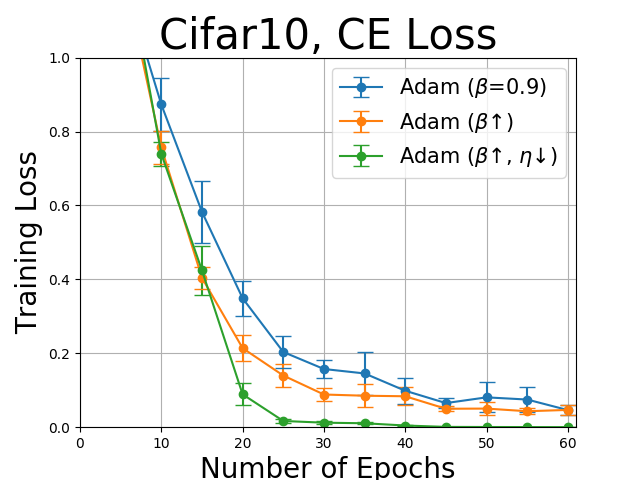
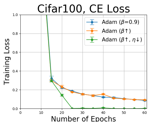
(a) Results on Image Data

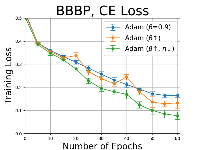
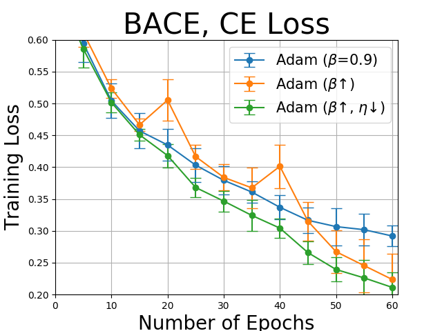
(b) Results on Molecule Data

Figure 1: Minimizing the CE loss

From Figure 1, we can see that in most cases decreasing $\beta$ especially together with decreasing $\eta$ can improve the convergence speed of the original Adam. This is reasonable because at the beginning the information in the current stochastic gradient is more valuable; hence using a relatively small $\beta$ is helpful for improving the convergence speed. As the solution gets closer to the optimal solution, the variance of the current stochastic gradient will affect the convergence; hence increasing $\beta$ will help reduce the variance of the gradient estimator. What is more, decreasing step size can further accelerate the optimization, which is also consistent with observations in practice of non-adaptive optimization algorithms.

6.2 Min-Max Problem

In this subsection, we consider the AUC maximization task for binary classification tasks. Specifically, we optimize a min-max formulated AUC maximization problem Ying et al. (2016); Liu et al. (2020b), whose formulation is given in the Appendix J.

The network we use for different data sets are the same as in the minimization problem. For Cifar10 and Cifar100, which has multiple classes, we merge half of their classes as the positive class and the others as the negative class. We compare our proposed algorithms PDSM and PDAda with baselines SGDA (Lin et al., 2020a), Epoch-SGDA Yan et al. (2020), PES-SGDA and PES-AdaGrad (Guo et al., 2020). SGDA is a single loop algorithm that updates the primal and dual variable in turn using stochastic gradients. Epoch-SGDA, PES-SGDA and PES-AdaGrad are double algorithms that decay step sizes after a number of iterations, where Epoch-SGDA decays the step size polynomially while the other two decay step size exponentially. The Epoch-SGDA and PES-SGDA update variables using stochastic gradient while PES-AdaGrad uses an AdaGrad style update. The second order momentum of PDAda is implemented as Adam, shown in Table 2.

For all algorithms, we tune initial $\eta_{x}$ and $\eta_{y}$ in $1e\text{-}5\sim 1e\text{-}2$. For PDSM and PDAda, we select the initial $\gamma=1-\beta$ from $\{0.99,0.9,0.5\}$. For the algorithms other than SGDA, we decay the step size and $\gamma$ every $E$ epochs where $E$ is chosen from $\{5,10,15,20,25,30\}$. In Epoch-SGDA, the step sizes of the $k$-th stage are $\frac{\eta_{x}}{k+1}$ and $\frac{\eta_{y}}{k+1}$. PES-SGDA, PES-AdaGrad, PDSM and PDAda decays step size and $\gamma$ by a factor $e$ tuned in $\{0.1,0.2,0.5,0.9\}$. Similar as before, we use a batch size of 32, and repeat the experiments 5 times and report the averaged results with standard deviation.

The results in Figure 2 have demonstrated that in most cases our PDAda and PDSM can outperform the non-adaptive algorithms i.e., SGDA, Epoch-SGDA and PES-SGDA, which indicates that the moving average estimator is helpful for improving the convergence. Also, our PDAda can outperform PES-AdaGrad. Note that the main differences between PDAda and PES-AdaGrad are that PDAda uses SEMA to estimate the gradient while PES-AdaGrad simply uses stochastic gradient.

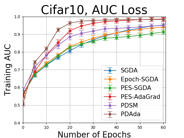
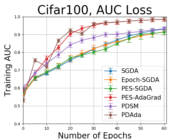
(a) Results on Image Data

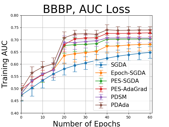
(b) Results on Molecule Data

Figure 2: Optimizing the Min-Max AUC loss

7 Conclusion

In this paper, we have considered the application of stochastic moving average estimators in non-convex optimization and established some interesting and important results. Our results not only bring some new insights to make the Adam method converge but also improve the state of the art results for stochastic non-convex strongly concave min-max optimization and stochastic bilevel optimization with a strongly convex lower-level problem. The oracle complexities established in this paper are optimal up to a logarithmic factor under a general stochastic unbiased oracle model.

A Stochastic Momentum Method

In the literature Yang et al. (2016), the stochastic heavy-ball method is written as:

$$\text{SHB:}\quad\left\{\begin{aligned} &\mathbf{v}^{\prime}_{t+1}=\beta^{\prime}\mathbf{v}^{\prime}_{t}-\eta^{\prime}\mathcal{O}_{F}(\mathbf{x}_{t})\\ &\mathbf{x}_{t+1}=\mathbf{x}_{t}+\mathbf{v}^{\prime}_{t+1},\quad t=0,\ldots,T.\end{aligned}\right.$$ (10)

To show the resemblance between the above update and the one in (2), we can transform them into one sequence update:

$$(\ref{eqn:sma}):\mathbf{x}_{t+1}=\mathbf{x}_{t}-\eta(1-\beta)\mathcal{O}_{F}(\mathbf{x}_{t})+\beta(\mathbf{x}_{t}-\mathbf{x}_{t-1})$$

$$\text{SHB: }\mathbf{x}_{t+1}=\mathbf{x}_{t}-\eta^{\prime}\mathcal{O}_{F}(\mathbf{x}_{t})+\beta^{\prime}(\mathbf{x}_{t}-\mathbf{x}_{t-1}).$$

We can see that SHB is equivalent to (2) with $\eta^{\prime}=\eta(1-\beta)$ and $\beta^{\prime}=\beta$.

B Proof of Lemma 5

Proof  Due to the smoothness of $F$, we can prove that under $\eta_{t}L_{F}\leq c_{l}/(2c_{u}^{2})$

$$F(\mathbf{x}_{t+1})\leq F(\mathbf{x}_{t})+\nabla F(\mathbf{x}_{t})^{\top}(\mathbf{x}_{t+1}-\mathbf{x}_{t})+\frac{L_{F}}{2}\|\mathbf{x}_{t+1}-\mathbf{x}_{t}\|^{2}$$

$$=F(\mathbf{x}_{t})-\nabla F(\mathbf{x}_{t})^{\top}(\tilde{\eta}_{t}\circ\mathbf{v}_{t+1})+\frac{L_{F}}{2}\|\tilde{\eta}_{t}\circ\mathbf{v}_{t+1}\|^{2}$$

$$=F(\mathbf{x}_{t})+\frac{1}{2}\|\sqrt{\tilde{\eta}_{t}}\circ(\nabla F(\mathbf{x}_{t})-\mathbf{v}_{t+1})\|^{2}-\frac{1}{2}\|\sqrt{\tilde{\eta}_{t}}\circ\nabla F(\mathbf{x}_{t})\|^{2}+(\frac{L_{F}}{2}\|\tilde{\eta}_{t}\circ\mathbf{v}_{t+1}\|^{2}-\frac{1}{2}\|\sqrt{\tilde{\eta}_{t}}\circ\mathbf{v}_{t+1}\|^{2})$$

$$\leq F(\mathbf{x}_{t})+\frac{\eta_{t}c_{u}}{2}\|\nabla F(\mathbf{x}_{t})-\mathbf{v}_{t+1}\|^{2}-\frac{\eta_{t}c_{l}}{2}\|\nabla F(\mathbf{x}_{t})\|^{2}+\frac{\eta_{t}^{2}c_{u}^{2}L_{F}-\eta_{t}c_{l}}{2}\|\mathbf{v}_{t+1}\|^{2}$$

$$\leq F(\mathbf{x}_{t})+\frac{\eta_{t}c_{u}}{2}\|\nabla F(\mathbf{x}_{t})-\mathbf{v}_{t+1}\|^{2}-\frac{\eta_{t}c_{l}}{2}\|\nabla F(\mathbf{x}_{t})\|^{2}-\frac{\eta_{t}c_{l}}{4}\|\mathbf{v}_{t+1}\|^{2}.$$

 

C Proof of Theorem 6

Proof  By applying Lemma 4 to $\mathbf{v}_{t+1}$, we have

$$\mathrm{E}_{t}[\Delta_{t+1}]\leq(1-\gamma)\Delta_{t}+2\gamma^{2}\sigma^{2}(1+c\|\nabla F(\mathbf{x}_{t+1})\|^{2})+\frac{L_{F}^{2}\|\mathbf{x}_{t+1}-\mathbf{x}_{t}\|^{2}}{\gamma}.$$

Hence we have,

$$\begin{split}\mathrm{E}\left[\sum_{t=0}^{T}\Delta_{t}\right]\leq\mathrm{E}\left[\sum_{t=0}^{T}\frac{\Delta_{t}-\Delta_{t+1}}{\gamma}+2\gamma\sigma^{2}(T+1)+2\gamma\sigma^{2}c\sum_{t=0}^{T}\|\nabla F(\mathbf{x}_{t+1})\|^{2}+\sum_{t=0}^{T}\frac{L_{F}^{2}\eta^{2}c_{u}^{2}\|\mathbf{v}_{t+1}\|^{2}}{\gamma^{2}}\right].\end{split}$$

Adding the above inequality with Lemma 5, we have

$$\frac{\eta c_{l}}{2}\mathrm{E}\left[\sum_{t=0}^{T}\|\nabla F(\mathbf{x}_{t})\|^{2}\right]\leq F(\mathbf{x}_{0})-F_{*}-\frac{\eta c_{l}}{4}\sum_{t=0}^{T}\mathrm{E}\|\mathbf{v}_{t+1}\|^{2}$$

$$+\frac{\eta c_{u}}{2}\mathrm{E}\left[\sum_{t=0}^{T}\frac{\Delta_{t}-\Delta_{t+1}}{\gamma}+2\gamma\sigma^{2}(T+1)+2\gamma\sigma^{2}c\sum_{t=0}^{T}\|\nabla F(\mathbf{x}_{t+1})\|^{2}+\sum_{t=0}^{T}\frac{L_{F}^{2}\eta^{2}c_{u}^{2}\|\mathbf{v}_{t+1}\|^{2}}{\gamma^{2}}\right]$$

$$\leq F(\mathbf{w}_{0})-F_{*}-\frac{\eta c_{l}}{4}\sum_{t=0}^{T}\mathrm{E}\|\mathbf{v}_{t+1}\|^{2}+\frac{\eta c_{u}}{2}\mathrm{E}\left[\frac{\Delta_{0}-\Delta_{T+1}}{\gamma}+2\gamma\sigma^{2}(T+1)+\sum_{t=0}^{T}\frac{L_{F}^{2}\eta^{2}c_{u}^{2}\|\mathbf{v}_{t+1}\|^{2}}{\gamma^{2}}\right]$$

$$+2\gamma\sigma^{2}c\sum_{t=0}^{T}\mathrm{E}\|\nabla F(\mathbf{x}_{t})-\nabla F(\mathbf{x}_{t})+\nabla F(\mathbf{x}_{t+1})\|^{2}$$

$$\leq F(\mathbf{w}_{0})-F_{*}-\frac{\eta c_{l}}{4}\sum_{t=0}^{T}\mathrm{E}\|\mathbf{v}_{t+1}\|^{2}+\frac{\eta c_{u}}{2}\mathrm{E}\left[\frac{\Delta_{0}-\Delta_{T+1}}{\gamma}+2\gamma\sigma^{2}(T+1)+\sum_{t=0}^{T}\frac{L_{F}^{2}\eta^{2}c_{u}^{2}\|\mathbf{v}_{t+1}\|^{2}}{\gamma^{2}}\right]$$

$$+2\eta c_{u}\gamma\sigma^{2}c\sum_{t=0}^{T}\mathrm{E}\|\nabla F(\mathbf{x}_{t})\|^{2}+2\eta c_{u}\gamma\sigma^{2}cL_{F}^{2}\eta^{2}c_{u}^{2}\mathrm{E}\|\mathbf{v}_{t+1}\|^{2}.$$

Let $L_{F}^{2}\eta^{2}c_{u}^{3}/(2\gamma^{2})\leq c_{l}/8$ (i.e., $\eta\leq\frac{\gamma\sqrt{c_{l}}}{2L_{F}\sqrt{c_{u}^{3}}})$ and $2c_{u}\gamma\sigma^{2}c\leq c_{l}/4$, $2\gamma\sigma^{2}cL_{F}^{2}\eta^{2}c_{u}^{3}\leq c_{l}/8$ (i.e, $\eta\leq\frac{1}{\sqrt{2}L_{F}c_{u}}$), we have

$$\begin{split}\frac{1}{T+1}\mathrm{E}\left[\sum_{t=0}^{T}\|\nabla F(\mathbf{x}_{t})\|^{2}\right]&\leq\frac{\Delta_{0}c_{u}}{\gamma Tc_{l}}+\frac{2(F(\mathbf{x}_{0})-F_{*})}{\eta c_{l}T}+2\gamma\sigma^{2}\frac{c_{u}}{c_{l}}+\frac{1}{2}\frac{1}{T+1}\mathrm{E}\bigg{[}\sum_{t=0}^{T}\|\nabla F(\mathbf{x}_{t})\|^{2}\bigg{]}.\end{split}$$

As a result,

$$\frac{1}{T+1}\mathrm{E}\left[\sum_{t=0}^{T}\|\nabla F(\mathbf{x}_{t})\|^{2}\right] \leq\frac{2\Delta_{0}c_{u}}{\gamma Tc_{l}}+\frac{4(F(\mathbf{x}_{0})-F_{*})}{\eta c_{l}T}+4\gamma\sigma^{2}\frac{c_{u}}{c_{l}}.$$

With $\gamma\leq\frac{\epsilon^{2}c_{l}}{12\sigma^{2}c_{u}}$, $T\geq\max\{\frac{6\Delta_{0}c_{u}}{\gamma\epsilon^{2}c_{l}},\frac{12\Delta_{F}}{\eta\epsilon^{2}c_{l}}\}$, we conclude the proof for the first part of the theorem. For the second part, we have

$$\mathrm{E}\left[\sum_{t=0}^{T}\Delta_{t}\right]\leq\frac{\Delta_{0}}{\gamma}+\gamma\sigma^{2}(T+1)+\frac{c_{l}}{2c_{u}}\mathrm{E}\bigg{[}\sum_{t=0}^{T}\|\nabla F(\mathbf{x}_{t})\|^{2}\bigg{]}+\mathrm{E}\bigg{[}\sum_{t=0}^{T}\frac{c_{l}}{2c_{u}}\|\mathbf{v}_{t+1}\|^{2}\bigg{]}$$

$$\leq\frac{\Delta_{0}}{\gamma}+2\gamma\sigma^{2}(T+1)+\frac{1}{2}\mathrm{E}\bigg{[}\sum_{t=0}^{T}\|\nabla F(\mathbf{x}_{t})\|^{2}\bigg{]}+\mathrm{E}\bigg{[}\sum_{t=0}^{T}\frac{1}{2}\Delta_{t}\bigg{]}$$

As a result,

$$\mathrm{E}\left[\frac{1}{T+1}\sum_{t=0}^{T}\Delta_{t}\right]\leq\frac{2\Delta_{0}}{\gamma T}+4\gamma\sigma^{2}+\mathrm{E}\bigg{[}\frac{1}{T+1}\sum_{t=0}^{T}\|\nabla F(\mathbf{x}_{t})\|^{2}\bigg{]}\leq 2\epsilon^{2}.$$

 

D Poof of Theorem 7

Proof  By applying Lemma 4 to $\mathbf{v}_{t+1}$, we have

$$\begin{split}\mathrm{E}_{t}[\Delta_{t+1}]\leq(1-\gamma_{t})\Delta_{t}+2\gamma_{t}^{2}\sigma^{2}(1+c\|\nabla F(\mathbf{x}_{t+1})\|^{2})+\frac{L_{F}^{2}\|\mathbf{x}_{t+1}-\mathbf{x}_{t}\|^{2}}{\gamma_{t}}.\end{split}$$ (11)

Hence we have

$$\begin{split}\mathrm{E}\left[\sum\limits_{t=0}^{T}\gamma_{t}\Delta_{t}\right]\leq\mathrm{E}\left[\sum\limits_{t=0}^{T}[\Delta_{t}-\Delta_{t+1}]+\sum\limits_{t=0}^{T}2\gamma_{t}^{2}\sigma^{2}(1+c\|\nabla F(\mathbf{x}_{t+1})\|^{2})+\sum\limits_{t=0}^{T}\frac{L_{F}^{2}\eta_{t}^{2}c_{u}^{2}\|\mathbf{v}_{t+1}\|^{2}}{\gamma_{t}}\right].\end{split}$$ (12)

Combining this with Lemma 5,

$$\begin{split}&\mathrm{E}\left[\sum\limits_{t=0}^{T}\frac{\eta_{t}c_{l}}{2}\|\nabla F(\mathbf{x}_{t})\|^{2}\right]\leq\sum\limits_{t=0}^{T}\mathrm{E}[F(\mathbf{x}_{t})-F(\mathbf{x}_{t+1})]-\sum\limits_{t=0}^{T}\frac{\eta_{t}c_{l}}{4}\mathrm{E}\|\mathbf{v}_{t+1}\|^{2}\\ &+\frac{\eta_{1}c_{u}}{2\gamma_{1}}\mathrm{E}\left[\sum\limits_{t=0}^{T}(\Delta_{t}-\Delta_{t+1})+\sum\limits_{t=0}^{T}2\gamma_{t}^{2}\sigma^{2}(1+c\|\nabla F(\mathbf{x}_{t+1})\|^{2})+\sum\limits_{t=0}^{T}\frac{L_{F}^{2}\eta_{t}^{2}c_{u}^{2}\|\mathbf{v}_{t+1}\|^{2}}{\gamma_{t}}\right]\Bigg{]}\\ &\leq F(\mathbf{x}_{0})-F_{*}-\sum\limits_{t=0}^{T}\frac{\eta_{t}c_{l}}{4}\mathrm{E}\|\mathbf{v}_{t+1}\|^{2}+\frac{\eta_{1}c_{u}\Delta_{0}}{2\gamma_{1}}+\frac{\eta_{1}c_{u}}{\gamma_{1}}\sum\limits_{t=0}^{T}\gamma_{t}^{2}\sigma^{2}+\frac{\eta_{1}c_{u}}{2\gamma_{1}}\sum\limits_{t=0}^{T}\frac{L_{F}^{2}\eta_{t}^{2}c_{u}^{2}\mathrm{E}\|\mathbf{v}_{t+1}\|^{2}}{\gamma_{t}}\\ &+\frac{\eta_{1}c_{u}}{2\gamma_{1}}\sum\limits_{t=0}^{T}2\gamma_{t}^{2}\sigma^{2}c\mathrm{E}\|\nabla F(\mathbf{x}_{t})-\nabla F(\mathbf{x}_{t})+\nabla F(\mathbf{x}_{t+1})\|^{2})\\ &\leq F(\mathbf{x}_{0})-F_{*}-\sum\limits_{t=0}^{T}\frac{\eta_{t}c_{l}}{4}\mathrm{E}\|\mathbf{v}_{t+1}\|^{2}+\frac{\eta_{1}c_{u}\Delta_{0}}{2\gamma_{1}}+\frac{\eta_{1}c_{u}}{\gamma_{1}}\sum\limits_{t=0}^{T}\gamma_{t}^{2}\sigma^{2}+\sum\limits_{t=0}^{T}\frac{L_{F}^{2}\eta_{t}^{2}c_{u}^{2}\mathrm{E}\|\mathbf{v}_{t+1}\|^{2}}{\gamma_{t}}\\ &+\frac{\eta_{1}c_{u}}{2\gamma_{1}}\left[\sum\limits_{t=0}^{T}4\gamma_{t}^{2}\sigma^{2}c\mathrm{E}\|\nabla F(\mathbf{x}_{t})\|^{2}+\sum\limits_{t=0}^{T}4\gamma_{t}^{2}\sigma^{2}cL_{F}^{2}\eta_{t}^{2}c_{u}^{2}\mathrm{E}\|\mathbf{v}_{t+1}\|^{2}\right]\\ &\leq F(\mathbf{x}_{0})-F_{*}+\frac{\eta_{1}c_{u}\Delta_{0}}{2\gamma_{1}}+\frac{c_{u}\eta_{1}}{\gamma_{1}}\sum\limits_{t=0}^{T}\gamma_{t}^{2}\sigma^{2}+\sum\limits_{t=0}^{T}\frac{\eta_{t}c_{l}}{4}\mathrm{E}\|\nabla F(\mathbf{x}_{t})\|^{2},\end{split}$$ (13)

where the last inequality holds because $\frac{2\eta_{1}c_{u}}{\gamma_{1}}\gamma_{t}^{2}\sigma^{2}c\leq\frac{\eta_{t}c_{l}}{4}$, $\frac{\eta_{1}}{2\gamma_{1}}\frac{L_{F}^{2}\eta_{t}^{2}c_{u}^{3}}{\gamma_{t}}\leq\frac{\eta_{t}c_{l}}{8}$ and $\frac{2\eta_{1}}{\gamma_{1}}\gamma_{t}^{2}\sigma^{2}cL_{F}^{2}\eta_{t}^{2}c_{u}^{3}\leq\frac{\eta_{t}c_{l}}{8}$ by the setting of $\eta_{t}$ and $\gamma_{t}$ in the theorem. Hence,

$$\begin{split}&\mathrm{E}\left[\sum\limits_{t=0}^{T}\eta_{T}c_{l}\|\nabla F(\mathbf{x}_{t})\|^{2}\right]\leq\mathrm{E}\left[\sum\limits_{t=0}^{T}\eta_{t}c_{l}\|\nabla F(\mathbf{x}_{t})\|^{2}\right]\\ &\leq 4(F(\mathbf{x}_{0})-F_{*})+\frac{2\eta_{1}c_{u}\Delta_{0}}{\gamma_{1}}+\sum\limits_{t=0}^{T}\frac{4c_{u}\eta_{1}}{\gamma_{1}}\gamma_{t}^{2}\sigma^{2}\\ &\leq 4(F(\mathbf{x}_{0})-F_{*})+\frac{\sqrt{c_{l}}\Delta_{0}}{L_{F}\sqrt{c_{u}}}+\sum\limits_{t=0}^{T}\frac{2\sqrt{c_{l}}}{L_{F}\sqrt{c_{u}}}\gamma_{t}^{2}\sigma^{2}.\end{split}$$ (14)

Thus,

$$\small\begin{split}\mathrm{E}\left[\frac{1}{T+1}\sum\limits_{t=0}^{T}\|\nabla F(\mathbf{x}_{t})\|^{2}\right]&\leq\frac{4(F(\mathbf{x}_{0})-F(\mathbf{x}_{*}))}{\eta_{T}c_{l}(T+1)}+\frac{\Delta_{0}}{L_{F}\sqrt{c_{l}c_{u}}\eta_{T}(T+1)}+\sum\limits_{t=0}^{T}\frac{2\gamma_{t}^{2}}{\eta_{T}L_{F}\sqrt{c_{l}c_{u}}(T+1)}\sigma^{2}\\ &\leq\frac{4\Delta_{F}}{\eta_{T}c_{l}(T+1)}+\frac{\Delta_{0}}{L_{F}\sqrt{c_{l}c_{u}}\eta_{T}(T+1)}+\frac{c_{l}^{2}}{32\eta_{T}\sigma^{2}L_{F}c^{2}\sqrt{c_{l}c_{u}^{5}}(T+1)}\ln(T+2).\end{split}$$

Setting $T\geq\widetilde{O}(\frac{c_{u}^{5}c^{2}L_{F}^{2}\sigma^{4}\Delta_{F}^{2}/c_{l}^{5}+\Delta_{0}^{2}c^{2}c_{u}^{4}\sigma^{4}/c_{l}^{4}+1/c}{\epsilon^{4}})$, we conclude the proof for the first part of the theorem. For the second part, we have

$$\begin{split}\mathrm{E}\left[\sum\limits_{t=0}^{T}\gamma_{t}\Delta_{t}\right]\leq\Delta_{0}+\frac{c_{l}^{2}}{16\sigma^{4}c^{2}c_{u}^{2}}\ln(T+2)+\frac{1}{2}\mathrm{E}\left[\sum\limits_{t=0}^{T}\gamma_{t}\|\nabla F(\mathbf{x}_{t})\|^{2}\right]+\mathrm{E}\left[\sum\limits_{t=0}^{T}\frac{1}{2}\gamma_{t}\Delta_{t}\right].\end{split}$$ (15)

Then,

$$\begin{split}\mathrm{E}\left[\frac{1}{T+1}\sum\limits_{t=0}^{T}\Delta_{t}\right]\leq\frac{2\Delta_{0}}{\gamma_{T}T}+\frac{c_{l}^{2}}{8\gamma_{T}\sigma^{4}c^{2}c_{u}^{2}(T+1)}\ln(T+2)+\frac{1}{2\gamma_{T}T}\mathrm{E}\left[\sum\limits_{t=0}^{T}\gamma_{t}\|\nabla F(\mathbf{x}_{t})\|^{2}\right],\end{split}$$ (16)

which concludes the proof of the second part of the theorem by the settings.  

E Proof of Theorem 8

Proof [Proof of Theorem 8] In this proof the subscript denote the epoch index $(1,...,K)$. Denote $\epsilon_{0}=\max\{F(\mathbf{x}_{0})-F_{*},\Delta_{0}\}$. We prove by induction. Assume that at the initialization of $k$-th stage, we have $\mathrm{E}[F(\mathbf{x}_{k})-F_{*}]\leq\epsilon_{k}$ and $\mathrm{E}\|\mathbf{v}_{k}-\nabla F(\mathbf{x}_{k})\|^{2}\leq\mu\epsilon_{k}$. By the analysis in Appendix C, we know that after the $k$-th stage,

$$\mathrm{E}[F(\mathbf{x}_{k+1})-F_{*}]\leq\frac{1}{2\mu}\mathrm{E}\left[\|\nabla F(\mathbf{x}_{k})\|^{2}\right] \leq\frac{\epsilon_{k}c_{u}}{\mu\gamma_{k}T_{k}c_{l}}+\frac{2\epsilon_{k}}{\mu\eta_{k}c_{l}T_{k}}+2\gamma_{k}\sigma^{2}\frac{c_{u}}{\mu c_{l}},$$

and

$$\mathrm{E}\left[\Delta_{k+1}\right]=\mathrm{E}\|\mathbf{v}_{k}-\nabla F(\mathbf{x}_{k})\|^{2}\leq\frac{2\epsilon_{k}}{\gamma_{k}T_{k}}+4\gamma_{k}\sigma^{2}+\mathrm{E}\left[\|\nabla F(\mathbf{x}_{k})\|^{2}\right].$$

By setting $\gamma_{k}\leq\frac{\mu c_{l}\epsilon_{k}}{24c_{u}\sigma^{2}}$, $\eta_{k}=\min\{\frac{\gamma_{k}\sqrt{c_{l}}}{2L_{F}\sqrt{c_{u}^{3}}},\frac{1}{\sqrt{2}L_{f}c_{u}}\}$ and $T_{k}=\max\{\frac{48c_{u}}{\mu\gamma_{k}c_{l}},\frac{1}{6\mu\eta_{k}c_{l}}\}$, then we have $\mathrm{E}[F(\mathbf{x}_{k+1})-F_{*}]\leq\epsilon_{k+1}=\epsilon_{k}/2$ and $\mathrm{E}\|\mathbf{v}_{k}-\nabla F(\mathbf{x}_{k})\|^{2}\leq\epsilon_{k+1}=\epsilon_{k}/2$, where we assume $\mu\leq 1$ without loss of generality.

Hence, after $K=\log(\epsilon_{0}/\epsilon)$ stages, it holds that $\mathrm{E}[F(\mathbf{x}_{K+1})-F_{*}]\leq\epsilon$ and $\mathrm{E}\|\mathbf{v}_{K}-\nabla F(\mathbf{x}_{K})\|^{2}\leq\epsilon$. The total number of iterations is $\widetilde{O}(\frac{1}{\mu^{2}\epsilon})$.

 

F Analysis of PDSM/PDAda with Strong Concavity

In this section, we analyze PDAda under Assumption 3 with the option $\mathcal{Y}\subseteq\mathbb{R}^{d^{\prime}}$ is a bounded or unbounded convex set and $f(\mathbf{x},\cdot)$ is $\lambda$-strongly concave for any $\mathbf{x}$, while analysis with dual side PL condition is discussed in Appendix G. We need the following lemmas.

Lemma 13

Suppose Assumption 2 holds. Considering the PDAdam update, with $\eta L_{F}\leq c_{l}/(2c_{u}^{2})$ we have

$$F(\mathbf{x}_{t+1})\leq F(\mathbf{x}_{t})+\frac{\eta_{x}c_{u}}{2}\|\nabla_{x}f(\mathbf{x}_{t},\mathbf{y}^{*}(\mathbf{x}_{t}))-\mathbf{u}_{t+1}\|^{2}-\frac{\eta_{x}c_{l}}{2}\|\nabla F(\mathbf{x}_{t})\|^{2}-\frac{\eta_{x}c_{l}}{4}\|\mathbf{u}_{t+1}\|^{2}.$$

Proof [Proof of Lemma 13] Denote $\tilde{\eta}_{x}=\eta_{x}s_{t}$. Due to the smoothness of $F$, we have that under $\eta_{x}\leq 1/(2L_{F})$

$$F(\mathbf{x}_{t+1})\leq F(\mathbf{x}_{t})+\nabla F(\mathbf{x}_{t})^{\top}(\mathbf{x}_{t+1}-\mathbf{x}_{t})+\frac{L_{F}}{2}\|\mathbf{x}_{t+1}-\mathbf{x}_{t}\|^{2}$$

$$=F(\mathbf{x}_{t})-\nabla F(\mathbf{x}_{t})^{\top}(\eta_{x}\circ\mathbf{v}_{t+1})+\frac{L_{F}}{2}\|\tilde{\eta}_{x}\circ\mathbf{v}_{t+1}\|^{2}$$

$$=F(\mathbf{x}_{t})+\frac{1}{2}\|\sqrt{\tilde{\eta}_{x}}\circ(\nabla_{x}f(\mathbf{x}_{t},\mathbf{y}^{*}(\mathbf{x}_{t}))-\mathbf{v}_{t+1})\|^{2}-\frac{1}{2}\|\sqrt{\tilde{\eta}_{x}}\circ\nabla F(\mathbf{x}_{t})\|^{2}+(\frac{L_{F}}{2}\|\tilde{\eta}_{x}\circ\mathbf{v}_{t+1}\|^{2}-\frac{1}{2}\|\sqrt{\tilde{\eta}_{x}}\circ\mathbf{v}_{t+1}\|^{2})$$

$$=F(\mathbf{x}_{t})+\frac{1}{2}\|\sqrt{\tilde{\eta}_{x}}\circ(\nabla_{x}f(\mathbf{x}_{t},\mathbf{y}^{*}(\mathbf{x}_{t}))-\mathbf{v}_{t+1})\|^{2}-\frac{1}{2}\|\sqrt{\tilde{\eta}_{x}}\circ\nabla F(\mathbf{x}_{t})\|^{2}+(\frac{\eta_{x}^{2}c_{u}^{2}L_{F}-\eta_{x}c_{l}}{2}\|\mathbf{v}_{t+1}\|^{2})$$

$$\leq F(\mathbf{x}_{t})+\frac{\eta_{x}c_{u}}{2}\|\nabla_{x}f(\mathbf{x}_{t},\mathbf{y}^{*}(\mathbf{x}_{t}))-\mathbf{v}_{t+1}\|^{2}-\frac{\eta_{x}c_{l}}{2}\|\nabla F(\mathbf{x}_{t})\|^{2}-\frac{\eta_{x}c_{l}}{4}\|\mathbf{v}_{t+1}\|^{2}.$$

 

Lemma 14

In Algorithm 3, it holds that

$$\begin{split}&\mathrm{E}\|\mathbf{v}_{t+1}-\nabla_{x}f(\mathbf{x}_{t},\mathbf{y}^{*}(\mathbf{x}_{t}))\|^{2}\\ &\leq(1-\frac{\gamma}{2})\mathrm{E}\|\mathbf{v}_{t}-\nabla_{x}f(\mathbf{x}_{t-1},\mathbf{y}^{*}(\mathbf{x}_{t-1}))\|^{2}+4\gamma^{2}\sigma^{2}+10\gamma L_{f}^{2}\mathrm{E}\|\mathbf{y}_{t}-\mathbf{y}^{*}(\mathbf{x}_{t})\|^{2}+\frac{2L_{F}^{2}}{\gamma}\mathrm{E}\|\mathbf{x}_{t}-\mathbf{x}_{t-1}\|^{2}.\end{split}$$

Proof [Proof of Lemma 14] Let $e_{t}=(1-\gamma)(\nabla F(\mathbf{x}_{t})-\nabla F(\mathbf{x}_{t-1}))=(1-\gamma)(\nabla_{x}f(\mathbf{x}_{t},\mathbf{y}^{*}(\mathbf{x}_{t}))-\nabla_{x}f(\mathbf{x}_{t-1},\mathbf{y}^{*}(\mathbf{x}_{t-1})))$. We have

$$\|e_{t}\|\leq(1-\gamma)\|\nabla F(\mathbf{x}_{t})-\nabla F(\mathbf{x}_{t-1})\|\leq(1-\gamma)L_{F}\|\mathbf{x}_{t}-\mathbf{x}_{t-1}\|.$$ (17)

and then it follows that

$$\begin{split}&\mathrm{E}_{t}\|\mathbf{v}_{t+1}-\nabla_{x}f(\mathbf{x}_{t},\mathbf{y}^{*}(\mathbf{x}_{t}))+e_{t}\|^{2}\\ &=\mathrm{E}\|(1-\gamma)(\mathbf{v}_{t}-\nabla_{x}f(\mathbf{x}_{t-1},\mathbf{y}^{*}(\mathbf{x}_{t-1})))+\gamma(\mathcal{O}_{x}(\mathbf{x}_{t},\mathbf{y}_{t})-\nabla_{x}f(\mathbf{x}_{t},\mathbf{y}^{*}(\mathbf{x}_{t})))\|^{2}\\ &=(1-\gamma)^{2}\mathrm{E}\|\mathbf{v}_{t}-\nabla_{x}f(\mathbf{x}_{t-1},\mathbf{y}^{*}(\mathbf{x}_{t-1}))\|^{2}+\gamma^{2}\mathrm{E}\|\mathcal{O}_{x}(\mathbf{x}_{t},\mathbf{y}_{t})-\nabla_{x}f(\mathbf{x}_{t},\mathbf{y}^{*}(\mathbf{x}_{t}))\|^{2}\\ &~{}~{}~{}+2(1-\gamma)\gamma\mathrm{E}\langle\mathbf{v}_{t}-\nabla_{x}f(\mathbf{x}_{t-1},\mathbf{y}^{*}(\mathbf{x}_{t-1})),\mathcal{O}_{x}(\mathbf{x}_{t},\mathbf{y}_{t})-\nabla_{x}f(\mathbf{x}_{t},\mathbf{y}_{t})\rangle.\\ &~{}~{}~{}+2(1-\gamma)\gamma\mathrm{E}\langle\mathbf{v}_{t}-\nabla_{x}f(\mathbf{x}_{t-1},\mathbf{y}^{*}(\mathbf{x}_{t-1})),\nabla_{x}f(\mathbf{x}_{t},\mathbf{y}_{t})-\nabla_{x}f(\mathbf{x}_{t},\mathbf{y}^{*}(\mathbf{x}_{t}))\rangle\\ &=(1-\gamma)^{2}\mathrm{E}\|\mathbf{v}_{t}-\nabla_{x}f(\mathbf{x}_{t-1},\mathbf{y}^{*}(\mathbf{x}_{t-1}))\|^{2}+\gamma^{2}\mathrm{E}\|\mathcal{O}_{x}(\mathbf{x}_{t},\mathbf{y}_{t})-\nabla_{x}f(\mathbf{x}_{t},\mathbf{y}^{*}(\mathbf{x}_{t}))\|^{2}\\ &~{}~{}~{}+2(1-\gamma)\gamma\mathrm{E}\langle\mathbf{v}_{t}-\nabla_{x}f(\mathbf{x}_{t-1},\mathbf{y}^{*}(\mathbf{x}_{t-1})),\nabla_{x}f(\mathbf{x}_{t},\mathbf{y}_{t})-\nabla_{x}f(\mathbf{x}_{t},\mathbf{y}^{*}(\mathbf{x}_{t}))\rangle\\ &\leq(1-\gamma)^{2}\mathrm{E}\|\mathbf{v}_{t}-\nabla_{x}f(\mathbf{x}_{t-1},\mathbf{y}^{*}(\mathbf{x}_{t-1}))\|^{2}+2\gamma^{2}\mathrm{E}\|\mathcal{O}_{x}(\mathbf{x}_{t},\mathbf{y}_{t})-\nabla_{x}f(\mathbf{x}_{t},\mathbf{y}_{t})\|^{2}\\ &~{}~{}~{}+2\gamma^{2}\mathrm{E}\|\nabla_{x}f(\mathbf{x}_{t},\mathbf{y}_{t})-\nabla_{x}f(\mathbf{x}_{t},\mathbf{y}^{*}(\mathbf{x}_{t}))\|^{2}+\frac{\gamma}{4}\mathrm{E}\|\mathbf{v}_{t}-\nabla_{x}f(\mathbf{x}_{t-1},\mathbf{y}^{*}(\mathbf{x}_{t-1}))\|^{2}\\ &~{}~{}~{}+4\gamma\mathrm{E}\|\nabla_{x}f(\mathbf{x}_{t},\mathbf{y}_{t})-\nabla_{x}f(\mathbf{x}_{t},\mathbf{y}^{*}(\mathbf{x}_{t}))\|^{2}\\ &\leq\left((1-\gamma)^{2}+\frac{\gamma}{4}\right)\mathrm{E}\|\mathbf{v}_{t}-\nabla_{x}f(\mathbf{x}_{t-1},\mathbf{y}^{*}(\mathbf{x}_{t-1}))\|^{2}+2\gamma^{2}\sigma^{2}+5\gamma L_{f}^{2}\|\mathbf{y}_{t}-\mathbf{y}^{*}(\mathbf{x}_{t})\|^{2}.\end{split}$$ (18)

We have with $\gamma<\frac{1}{4}$,

$$\begin{split}&\mathrm{E}\|\mathbf{v}_{t+1}-\nabla_{x}f(\mathbf{x}_{t},\mathbf{y}^{*}(\mathbf{x}_{t}))\|^{2}\leq(1+\gamma)\mathrm{E}\|\mathbf{v}_{t+1}-\nabla_{x}f(\mathbf{x}_{t},\mathbf{y}^{*}(\mathbf{x}_{t}))+e_{t}\|^{2}+(1+1/\gamma)\|e_{t}\|^{2}\\ &\leq(1-\frac{\gamma}{2})\mathrm{E}\|\mathbf{v}_{t}-\nabla_{x}f(\mathbf{x}_{t-1},\mathbf{y}^{*}(\mathbf{x}_{t-1}))\|^{2}+2(1+\gamma)\gamma^{2}\sigma^{2}+5(1+\gamma)\gamma L_{f}^{2}\mathrm{E}\|\mathbf{y}_{t}-\mathbf{y}^{*}(\mathbf{x}_{t})\|^{2}\\ &~{}~{}~{}+(1+1/\gamma)(1-\gamma)^{2}L_{F}^{2}\|\mathbf{x}_{t}-\mathbf{x}_{t-1}\|^{2}\\ &\leq(1-\frac{\gamma}{2})\mathrm{E}\|\mathbf{v}_{t}-\nabla_{x}f(\mathbf{x}_{t-1},\mathbf{y}^{*}(\mathbf{x}_{t-1}))\|^{2}+4\gamma^{2}\sigma^{2}+10\gamma L_{f}^{2}\mathrm{E}\|\mathbf{y}_{t}-\mathbf{y}^{*}(\mathbf{x}_{t})\|^{2}+\frac{2L_{F}^{2}}{\gamma}\mathrm{E}\|\mathbf{x}_{t}-\mathbf{x}_{t-1}\|^{2}.\end{split}$$

 

Lemma 15

Suppose Assumption 3 holds with the option $\mathcal{Y}\subseteq\mathbb{R}^{d^{\prime}}$ is a bounded or unbounded convex set and $f(\mathbf{x},\cdot)$ is $\lambda$-strongly concave for any $\mathbf{x}$. With $\mathbf{y}_{t+1}=\Pi_{\mathcal{Y}}[\mathbf{y}_{t}+\eta_{y}\mathcal{O}_{fy}(\mathbf{x}_{t},\mathbf{y}_{t})]$, $\eta_{y}\leq\lambda/L_{f}^{2}$ and $\kappa=L_{f}/\lambda$, we have

$$\begin{split}\mathrm{E}\|\mathbf{y}_{t+1}-\mathbf{y}^{*}(\mathbf{x}_{t+1})\|^{2}&\leq(1-\frac{\eta_{y}\lambda}{2})\mathrm{E}\|\mathbf{y}_{t}-\mathbf{y}^{*}(\mathbf{x}_{t})\|^{2}+2\eta_{y}^{2}\sigma^{2}+\frac{4\kappa^{2}}{\eta_{y}\lambda}\|\mathbf{x}_{t}-\mathbf{x}_{t+1}\|^{2}.\end{split}$$

Proof [Proof of Lemma 15] Since $\mathbf{y}^{*}(\mathbf{x}_{t})=\Pi_{\mathcal{Y}}[\mathbf{y}^{*}(\mathbf{x}_{t})+\eta_{y}\nabla_{y}f(\mathbf{x}_{t},\mathbf{y}^{*}(\mathbf{x}_{t}))]$ and $\mathbf{y}_{t+1}=\Pi_{\mathcal{Y}}[\mathbf{y}_{t}+\eta_{y}\mathcal{O}_{y}(\mathbf{x}_{t},\mathbf{y}_{t})]$, we have

$$\begin{split}&\mathrm{E}\|\mathbf{y}_{t+1}-\mathbf{y}^{*}(\mathbf{x}_{t})\|^{2}=\|\Pi_{y}[\mathbf{y}_{t}+\eta_{y}\mathcal{O}_{y}(\mathbf{x}_{t},\mathbf{y}_{t})]-\Pi_{y}[\mathbf{y}^{*}(\mathbf{x}_{t})+\eta_{y}\nabla_{y}f(\mathbf{x}_{t},\mathbf{y}^{*}(\mathbf{x}_{t}))]\|^{2}\\ &\leq\mathrm{E}\|[\mathbf{y}_{t}+\eta_{y}\mathcal{O}_{y}(\mathbf{x}_{t},\mathbf{y}_{t})]-[\mathbf{y}^{*}(\mathbf{x}_{t})+\eta_{y}\nabla_{y}f(\mathbf{x}_{t},\mathbf{y}^{*}(\mathbf{x}_{t}))]\|^{2}\\ &=\mathrm{E}\|[\mathbf{y}_{t}+\eta_{y}\mathcal{O}_{y}(\mathbf{x}_{t},\mathbf{y}_{t})-\eta_{y}\nabla f(\mathbf{x}_{t},\mathbf{y}_{t})+\eta_{y}\nabla f(\mathbf{x}_{t},\mathbf{y}_{t})]-[\mathbf{y}^{*}(\mathbf{x}_{t})+\eta_{y}\nabla_{y}f(\mathbf{x}_{t},\mathbf{y}^{*}(\mathbf{x}_{t}))]\|^{2}\\ &=\mathrm{E}\|[\mathbf{y}_{t}+\eta_{y}\nabla f(\mathbf{x}_{t},\mathbf{y}_{t})]-[\mathbf{y}^{*}(\mathbf{x}_{t})+\eta_{y}\nabla_{y}f(\mathbf{x}_{t},\mathbf{y}^{*}(\mathbf{x}_{t}))]\|^{2}+\eta_{y}^{2}\mathrm{E}\|\mathcal{O}_{y}(\mathbf{x}_{t},\mathbf{y}_{t})-\nabla f(\mathbf{x}_{t},\mathbf{y}_{t})\|^{2}\\ &+2\eta_{y}\mathrm{E}\langle[\mathbf{y}_{t}+\eta_{y}\nabla f(\mathbf{x}_{t},\mathbf{y}_{t})]-[\mathbf{y}^{*}(\mathbf{x}_{t})+\eta_{y}\nabla_{y}f(\mathbf{x}_{t},\mathbf{y}^{*}(\mathbf{x}_{t}))],\nabla\mathcal{O}_{y}(\mathbf{x}_{t},\mathbf{y}_{t})-f(\mathbf{x}_{t},\mathbf{y}_{t})\rangle\\ &\leq\mathrm{E}\|[\mathbf{y}_{t}+\eta_{y}\nabla f(\mathbf{x}_{t},\mathbf{y}_{t})]-[\mathbf{y}^{*}(\mathbf{x}_{t})+\eta_{y}\nabla_{y}f(\mathbf{x}_{t},\mathbf{y}^{*}(\mathbf{x}_{t}))]\|^{2}+\eta_{y}^{2}\sigma^{2},\end{split}$$

where

$$\begin{split}&\mathrm{E}\|[\mathbf{y}_{t}+\eta_{y}\nabla f(\mathbf{x}_{t},\mathbf{y}_{t})]-[\mathbf{y}^{*}(\mathbf{x}_{t})+\eta_{y}\nabla_{y}f(\mathbf{x}_{t},\mathbf{y}^{*}(\mathbf{x}_{t}))]\|^{2}\\ &=\mathrm{E}\|\mathbf{y}_{t}-\mathbf{y}^{*}(\mathbf{x}_{t})\|^{2}+\eta_{y}^{2}\mathrm{E}\|\nabla f(\mathbf{x}_{t},\mathbf{y}_{t})-\nabla_{y}f(\mathbf{x}_{t},\mathbf{y}^{*}(\mathbf{x}_{t}))\|^{2}\\ &~{}~{}~{}+2\eta_{y}\mathrm{E}\langle\mathbf{y}_{t}-\mathbf{y}^{*}(\mathbf{x}_{t}),\nabla_{y}f(\mathbf{x}_{t},\mathbf{y}_{t})-\nabla_{y}f(\mathbf{x}_{t},\mathbf{y}^{*}(\mathbf{x}_{t}))\rangle\\ &\leq\mathrm{E}\|\mathbf{y}_{t}-\mathbf{y}^{*}(\mathbf{x}_{t})\|^{2}+\eta_{y}^{2}\mathrm{E}\|\nabla f(\mathbf{x}_{t},\mathbf{y}_{t})-\nabla_{y}f(\mathbf{x}_{t},\mathbf{y}^{*}(\mathbf{x}_{t}))\|^{2}-2\eta_{y}\lambda\mathrm{E}\|\mathbf{y}_{t}-\mathbf{y}^{*}(\mathbf{x}_{t})\|^{2}\\ &\leq(1-\eta_{y}\lambda)\mathrm{E}\|\mathbf{y}_{t}-\mathbf{y}^{*}(\mathbf{x}_{t})\|^{2},\end{split}$$ (19)

where the first inequality uses strong monotone inequality as $-f(\mathbf{x}_{t},\cdot)$ is $\lambda$-strongly convex and the second inequality uses the setting $\eta_{y}\leq\lambda/L_{f}^{2}$. Then,

$$\begin{split}&\mathrm{E}\|\mathbf{y}_{t+1}-\mathbf{y}^{*}(\mathbf{x}_{t+1})\|^{2}\leq(1+\frac{\eta_{y}\lambda}{2})\mathrm{E}\|\mathbf{y}_{t+1}-\mathbf{y}^{*}(\mathbf{x}_{t})\|^{2}+(1+\frac{2}{\eta_{y}\lambda})\mathrm{E}\|\mathbf{y}^{*}(\mathbf{x}_{t})-\mathbf{y}^{*}(\mathbf{x}_{t+1})\|^{2}\\ &\leq(1+\frac{\eta_{y}\lambda}{2})(1-\eta_{y}\lambda)\mathrm{E}\|\mathbf{y}_{t}-\mathbf{y}^{*}(\mathbf{x}_{t})\|^{2}+(1+\frac{\eta_{y}\lambda}{2})\eta_{y}^{2}\sigma^{2}+\frac{4}{\eta_{y}\lambda}\kappa^{2}\mathrm{E}\|\mathbf{x}_{t}-\mathbf{x}_{t+1}\|^{2}\\ &\leq(1-\frac{\eta_{y}\lambda}{2})\mathrm{E}\|\mathbf{y}_{t}-\mathbf{y}^{*}(\mathbf{x}_{t})\|^{2}+2\eta_{y}^{2}\sigma^{2}+\frac{4\kappa^{2}}{\eta_{y}\lambda}\mathrm{E}\|\mathbf{x}_{t}-\mathbf{x}_{t+1}\|^{2},\end{split}$$ (20)

where the first inequality uses the property that $\mathbf{y}^{*}(\cdot)$ is $\kappa$-Lipschitz (Lemma 4.3 of (Lin et al., 2020a)).  

Then we are ready to prove Theorem 9 in the case $\mathcal{Y}\subseteq\mathbb{R}^{d^{\prime}}$ is a bounded or unbounded convex set and $f(\mathbf{x},\cdot)$ is $\lambda$-strongly concave for any $\mathbf{x}$.

Proof [Proof of Theorem 9] Below, we denote by $\Delta_{x,t}=\|\nabla_{x}f(\mathbf{x}_{t},\mathbf{y}^{*}(\mathbf{x}_{t}))-\mathbf{v}_{t+1}\|^{2}$. By applying Lemma 14, we have

$$\mathrm{E}\bigg{[}\sum_{t=0}^{T}\Delta_{x,t}\bigg{]}\leq\frac{2\mathrm{E}[\Delta_{x,0}]}{\gamma}+8\gamma\sigma^{2}(T+1)+20L_{f}^{2}\mathrm{E}\left[\sum_{t=1}^{T+1}\delta_{y,t}\right]+\mathrm{E}\bigg{[}\sum_{t=0}^{T}\frac{4L_{F}^{2}\eta_{x}^{2}c_{u}^{2}\|\mathbf{v}_{t+1}\|^{2})}{\gamma^{2}}\bigg{]}.$$

Applying Lemma 15, we have

$$\mathrm{E}\bigg{[}\sum_{t=0}^{T}\delta_{y,t}\bigg{]}\leq\frac{2}{\eta_{y}\lambda}\mathrm{E}[\delta_{y,0}]+\frac{4\eta_{y}\sigma^{2}(T+1)}{\lambda}+\frac{8\kappa^{2}\eta_{x}^{2}c_{u}^{2}}{\eta_{y}^{2}\lambda^{2}}\sum\limits_{t=0}^{T}\|\mathbf{v}_{t+1}\|^{2}.$$

and

$$\mathrm{E}\bigg{[}\sum_{t=1}^{T+1}\delta_{y,t}\bigg{]}\leq\frac{2}{\eta_{y}\lambda}\mathrm{E}[\delta_{y,0}]+\frac{4\eta_{y}\sigma^{2}(T+1)}{\lambda}+\frac{8\kappa^{2}\eta_{x}^{2}c_{u}^{2}}{\eta_{y}^{2}\lambda^{2}}\sum\limits_{t=0}^{T}\|\mathbf{v}_{t+1}\|^{2}.$$

Combining the above two bounds with Lemma 13, we have

$$\mathrm{E}\bigg{[}\sum_{t=0}^{T}\|\nabla F(\mathbf{x}_{t})\|^{2}\bigg{]}\leq\frac{2(F(\mathbf{x}_{0})-F(\mathbf{x}_{T+1}))}{\eta_{x}c_{l}}+\frac{c_{u}}{c_{l}}\mathrm{E}\left[\sum\limits_{t=0}^{T}\Delta_{x,t}\right]-\frac{1}{2}\sum\limits_{t=0}^{T}\|\mathbf{v}_{t+1}\|^{2}$$

$$\leq\frac{2(F(\mathbf{x}_{0})-F_{*})}{\eta_{x}c_{l}}+\frac{2c_{u}\mathrm{E}[\Delta_{x,0}]}{\gamma c_{l}}+\frac{8c_{u}\gamma\sigma^{2}(T+1)}{c_{l}}+\frac{20c_{u}L_{f}^{2}}{c_{l}}\mathrm{E}\left[\sum\limits_{t=1}^{T+1}\delta_{y,t}\right]$$

$$~{}~{}~{}+\mathrm{E}\bigg{[}\sum_{t=0}^{T}\frac{4c_{u}^{3}L_{F}^{2}\eta_{x}^{2}\|\mathbf{v}_{t+1}\|^{2})}{c_{l}\gamma^{2}}\bigg{]}-\frac{1}{2}\sum\limits_{t=0}^{T}\|\mathbf{v}_{t+1}\|^{2}$$

$$\leq\frac{2(F(\mathbf{x}_{0})-F_{*})}{\eta_{x}c_{l}}+\frac{2c_{u}\mathrm{E}[\Delta_{x,0}]}{\gamma c_{l}}+\frac{8c_{u}\gamma\sigma^{2}(T+1)}{c_{l}}+\frac{40c_{u}L_{f}^{2}}{c_{l}\eta_{y}\lambda}\mathrm{E}[\delta_{y,0}]+\frac{80c_{u}L_{f}^{2}\eta_{y}\sigma^{2}(T+1)}{c_{l}\lambda}$$

$$~{}~{}~{}+\bigg{(}\frac{160c_{u}^{3}L_{f}^{2}\kappa^{2}\eta_{x}^{2}}{c_{l}\eta_{y}^{2}\lambda^{2}}+\frac{4c_{u}^{3}L_{F}^{2}\eta_{x}^{2}}{c_{l}\gamma^{2}}-\frac{1}{2}\bigg{)}\mathrm{E}\left[\sum\limits_{t=0}^{T}\|\mathbf{v}_{t+1}\|^{2}\right]$$

$$\leq\frac{2(F(\mathbf{x}_{0})-F_{*})}{\eta_{x}c_{l}}+\frac{2c_{u}\mathrm{E}[\Delta_{x,0}]}{\gamma c_{l}}+\frac{8c_{u}\gamma\sigma^{2}(T+1)}{c_{l}}+\frac{40c_{u}L_{f}^{2}}{c_{l}\eta_{y}\lambda}\mathrm{E}[\delta_{y,0}]+\frac{80c_{u}L_{f}^{2}\eta_{y}\sigma^{2}(T+1)}{c_{l}\lambda},$$

where the last inequality uses the fact $\bigg{(}\frac{160c_{u}^{3}(L_{f}^{2}\kappa^{2}\eta_{x}^{2}}{c_{l}\eta_{y}^{2}\lambda^{2}}+\frac{4c_{u}^{3}L_{F}^{2}\eta_{x}^{2}}{c_{l}\gamma^{2}}-\frac{1}{2}\bigg{)}\leq-\frac{1}{4}\leq 0$ due to

$$\eta_{x}\leq\sqrt{\frac{c_{l}}{c_{u}^{3}}}\min\{\frac{\eta_{y}\lambda}{48L_{f}\kappa},\frac{\gamma}{8L_{F}}\}.$$

Hence, we have

$$\frac{1}{T+1}\mathrm{E}\bigg{[}\sum_{t=0}^{T}\|\nabla F(\mathbf{x}_{t})\|^{2}\bigg{]}\leq \frac{2\Delta_{F}}{\eta_{x}c_{l}T}+\frac{2c_{u}\mathrm{E}[\Delta_{x,0}]}{\gamma c_{l}T}+\frac{8c_{u}\gamma\sigma^{2}}{c_{l}}+\frac{40c_{u}L_{f}^{2}}{c_{l}\eta_{y}\lambda T}\mathrm{E}[\delta_{y,0}]+\frac{80c_{u}L_{f}^{2}\eta_{y}\sigma^{2}}{c_{l}\lambda}.$$

With $\gamma\leq\frac{c_{l}\epsilon^{2}}{40c_{u}\sigma^{2}},\eta_{y}\leq\frac{c_{l}\lambda\epsilon^{2}}{400c_{u}L_{f}^{2}\sigma^{2}}$, and $T\geq\max\{\frac{10\Delta_{F}}{\eta_{x}c_{l}\epsilon^{2}},\frac{10c_{u}\mathrm{E}{[\Delta_{x,0}]}}{\gamma c_{l}},\frac{200c_{u}L^{2}_{f}}{c_{l}\eta_{y}\lambda\epsilon^{2}}\}$, we have

$$\frac{1}{T+1}\mathrm{E}\bigg{[}\sum_{t=0}^{T}\|\nabla F(\mathbf{x}_{t})\|^{2}\bigg{]}\leq\epsilon^{2},$$

which concludes the first part of the theorem. For the second part, we have

$$\small\begin{split}&\mathrm{E}\left[\sum\limits_{t=0}^{T}(\Delta_{x,t}+L_{f}^{2}\delta_{y,t})\right]\\ &\leq\frac{2\mathrm{E}[\Delta_{x,0}]}{\gamma}+8\gamma\sigma^{2}(T+1)+\mathrm{E}\left[\sum\limits_{t=0}^{T}(20L_{f}^{2}\delta_{y,t+1}+L_{f}^{2}\delta_{y,t})\right]+\mathrm{E}\bigg{[}\sum_{t=0}^{T}\frac{4L_{F}^{2}c_{u}^{2}\eta_{x}^{2}\|\mathbf{v}_{t+1}\|^{2})}{\gamma^{2}}\bigg{]}\\ &\leq\frac{2\mathrm{E}[\Delta_{x,0}]}{\gamma}+8\gamma\sigma^{2}(T+1)+\frac{42L_{f}^{2}}{\eta_{y}\lambda}\mathrm{E}[\delta_{y,0}]+\frac{84L_{f}^{2}\eta_{y}\sigma^{2}(T+1)}{\lambda}+\frac{168L_{f}^{2}\kappa^{2}\eta_{x}^{2}c_{u}^{2}}{\eta_{y}^{2}\lambda^{2}}\sum\limits_{t=0}^{T}\|\mathbf{v}_{t+1}\|^{2}\\ &+\mathrm{E}\bigg{[}\sum_{t=0}^{T}\frac{4L_{F}^{2}\eta_{x}^{2}c_{u}^{2}\|\mathbf{v}_{t+1}\|^{2}}{\gamma^{2}}\bigg{]}\\ &\leq\frac{2\mathrm{E}[\Delta_{x,0}]}{\gamma}+8\gamma\sigma^{2}(T+1)+\frac{42L_{f}^{2}}{\eta_{y}\lambda}\mathrm{E}[\delta_{y,0}]+\frac{84L_{f}^{2}\eta_{y}\sigma^{2}(T+1)}{\lambda}\\ &+\frac{1}{3}\mathrm{E}\left[\sum\limits_{t=0}^{T}\|\mathbf{v}_{t+1}-\nabla_{x}f(\mathbf{x}_{t},\mathbf{y}^{*}(\mathbf{x}_{t}))-\nabla F(\mathbf{x}_{t})\|^{2}\right]\\ &\leq\frac{2\mathrm{E}[\Delta_{x,0}]}{\gamma}+8\gamma\sigma^{2}(T+1)+\frac{42L_{f}^{2}}{\eta_{y}\lambda}\mathrm{E}[\delta_{y,0}]+\frac{84L_{f}^{2}\eta_{y}\sigma^{2}(T+1)}{\lambda}\\ &+\frac{2}{3}\mathrm{E}\left[\sum\limits_{t=0}^{T}\Delta_{x,t}+\|\nabla F(\mathbf{x}_{t})\|^{2}\right]\end{split}$$ (21)

Thus,

$$\begin{split}\frac{1}{T+1}\mathrm{E}\left[\sum\limits_{t=0}^{T}(\Delta_{x,t}+L_{f}^{2}\delta_{y,t})\right]\leq 5\epsilon^{2}.\end{split}$$ (22)

 

G Analysis of PDSM/PDAda without Strong Concavity

Note that the analysis of PDSM/PDAda in the previous section uses strong concavity mainly in proving Lemma 15. Therefore, we only need to provide a similar bound as in 15 then we can fit in the framework of the previous section.

Lemma 16 (Lemma A.3 of (Nouiehed et al., 2019))

Under Assumption 3, with $\kappa=L_{f}/\lambda$, for any $\mathbf{x}_{1},\mathbf{x}_{2}$, and $\mathbf{y}^{*}(\mathbf{x}_{1})\in\arg\max_{y^{\prime}}f(\mathbf{x}_{1},\mathbf{y}^{\prime})$, there exists some $\mathbf{y}^{*}(\mathbf{x}_{2})\in\arg\max_{y^{\prime}}f(\mathbf{x}_{2},\mathbf{y}^{\prime})$ such that

$$\|\mathbf{y}^{*}(\mathbf{x}_{1})-\mathbf{y}^{*}(\mathbf{x}_{2})\|\leq\kappa\|\mathbf{x}_{1}-\mathbf{x}_{2}\|.$$ (23)

Note that in the further analysis we need to properly choose all the $\mathbf{y}^{*}(\mathbf{x}_{t})$ as required by Lemma 16, i.e., given $\mathbf{y}^{*}(\mathbf{x}_{t})$, $\mathbf{y}^{*}(\mathbf{x}_{t+1})$ is chosen from the set $\arg\max_{y^{\prime}}f(\mathbf{x}_{t+1},\mathbf{y}^{\prime})$ such that $\|\mathbf{y}^{*}(\mathbf{x}_{t})-\mathbf{y}^{*}(\mathbf{x}_{t+1})\|\leq\kappa\|\mathbf{x}_{t}-\mathbf{x}_{t+1}\|$. Then we can prove the following lemma.

Lemma 17

Suppose Assumption 3 holds. With $\mathbf{y}_{t+1}=\mathbf{y}_{t}+\eta_{y}\mathcal{O}_{fy}(\mathbf{x}_{t},\mathbf{y}_{t})$, $\eta_{y}\leq\lambda/(2L_{f}^{2})$ and $\kappa=L_{f}/\lambda$, we have that for any $\mathbf{y}^{*}(\mathbf{x}_{t})\in\arg\max_{y^{\prime}}f(\mathbf{x}_{t},\mathbf{y}^{\prime})$ there is a $\mathbf{y}^{*}(\mathbf{x}_{t+1})\in\arg\max_{y^{\prime}}f(\mathbf{x}_{t+1},\mathbf{y}^{\prime})$ such that

$$\begin{split}\mathrm{E}\|\mathbf{y}_{t+1}-\mathbf{y}^{*}(\mathbf{x}_{t+1})\|^{2}&\leq(1-\frac{\eta_{y}\lambda}{4})\mathrm{E}\|\mathbf{y}_{t}-\mathbf{y}^{*}(\mathbf{x}_{t})\|^{2}+2\eta_{y}^{2}\sigma^{2}+\frac{8\kappa^{2}}{\eta_{y}\lambda}\|\mathbf{x}_{t}-\mathbf{x}_{t+1}\|^{2}.\end{split}$$

Proof [Proof of Lemma 17] It holds that

$$\begin{split}&\mathrm{E}\|\mathbf{y}_{t+1}-\mathbf{y}^{*}(\mathbf{x}_{t})\|^{2}=\|\mathbf{y}_{t}+\eta_{y}\mathcal{O}_{y}(\mathbf{x}_{t},\mathbf{y}_{t})-\mathbf{y}^{*}(\mathbf{x}_{t})]\|^{2}\\ &=\mathrm{E}\|[\mathbf{y}_{t}+\eta_{y}\mathcal{O}_{y}(\mathbf{x}_{t},\mathbf{y}_{t})]-[\mathbf{y}^{*}(\mathbf{x}_{t})+\eta_{y}\nabla_{y}f(\mathbf{x}_{t},\mathbf{y}^{*}(\mathbf{x}_{t}))]\|^{2}\\ &=\mathrm{E}\|[\mathbf{y}_{t}+\eta_{y}\mathcal{O}_{y}(\mathbf{x}_{t},\mathbf{y}_{t})-\eta_{y}\nabla f(\mathbf{x}_{t},\mathbf{y}_{t})+\eta_{y}\nabla f(\mathbf{x}_{t},\mathbf{y}_{t})]-[\mathbf{y}^{*}(\mathbf{x}_{t})+\eta_{y}\nabla_{y}f(\mathbf{x}_{t},\mathbf{y}^{*}(\mathbf{x}_{t}))]\|^{2}\\ &=\mathrm{E}\|[\mathbf{y}_{t}+\eta_{y}\nabla f(\mathbf{x}_{t},\mathbf{y}_{t})]-[\mathbf{y}^{*}(\mathbf{x}_{t})+\eta_{y}\nabla_{y}f(\mathbf{x}_{t},\mathbf{y}^{*}(\mathbf{x}_{t}))]\|^{2}+\eta_{y}^{2}\mathrm{E}\|\mathcal{O}_{y}(\mathbf{x}_{t},\mathbf{y}_{t})-\nabla f(\mathbf{x}_{t},\mathbf{y}_{t})\|^{2}\\ &+2\eta_{y}\mathrm{E}\langle[\mathbf{y}_{t}+\eta_{y}\nabla f(\mathbf{x}_{t},\mathbf{y}_{t})]-[\mathbf{y}^{*}(\mathbf{x}_{t})+\eta_{y}\nabla_{y}f(\mathbf{x}_{t},\mathbf{y}^{*}(\mathbf{x}_{t}))],\nabla\mathcal{O}_{y}(\mathbf{x}_{t},\mathbf{y}_{t})-f(\mathbf{x}_{t},\mathbf{y}_{t})\rangle\\ &\leq\mathrm{E}\|[\mathbf{y}_{t}+\eta_{y}\nabla f(\mathbf{x}_{t},\mathbf{y}_{t})]-[\mathbf{y}^{*}(\mathbf{x}_{t})+\eta_{y}\nabla_{y}f(\mathbf{x}_{t},\mathbf{y}^{*}(\mathbf{x}_{t}))]\|^{2}+\eta_{y}^{2}\sigma^{2},\end{split}$$

where

$$\begin{split}&\mathrm{E}\|[\mathbf{y}_{t}+\eta_{y}\nabla f(\mathbf{x}_{t},\mathbf{y}_{t})]-[\mathbf{y}^{*}(\mathbf{x}_{t})+\eta_{y}\nabla_{y}f(\mathbf{x}_{t},\mathbf{y}^{*}(\mathbf{x}_{t}))]\|^{2}\\ &=\mathrm{E}\|\mathbf{y}_{t}-\mathbf{y}^{*}(\mathbf{x}_{t})\|^{2}+\eta_{y}^{2}\mathrm{E}\|\nabla f(\mathbf{x}_{t},\mathbf{y}_{t})-\nabla_{y}f(\mathbf{x}_{t},\mathbf{y}^{*}(\mathbf{x}_{t}))\|^{2}+2\eta_{y}\mathrm{E}\langle\mathbf{y}_{t}-\mathbf{y}^{*}(\mathbf{x}_{t}),\nabla f(\mathbf{x}_{t},\mathbf{y}_{t})\rangle\\ &\leq\mathrm{E}\|\mathbf{y}_{t}-\mathbf{y}^{*}(\mathbf{x}_{t})\|^{2}+\eta_{y}^{2}\mathrm{E}\|\nabla f(\mathbf{x}_{t},\mathbf{y}_{t})-\nabla_{y}f(\mathbf{x}_{t},\mathbf{y}^{*}(\mathbf{x}_{t}))\|^{2}+2\eta_{y}(f(\mathbf{x}_{t},\mathbf{y}_{t})-f(\mathbf{x}_{t},\mathbf{y}^{*}(\mathbf{x}_{t}))\\ &\leq\mathrm{E}\|\mathbf{y}_{t}-\mathbf{y}^{*}(\mathbf{x}_{t})\|^{2}+\eta_{y}^{2}\mathrm{E}\|\nabla f(\mathbf{x}_{t},\mathbf{y}_{t})-\nabla_{y}f(\mathbf{x}_{t},\mathbf{y}^{*}(\mathbf{x}_{t}))\|^{2}-\eta_{y}\lambda\mathrm{E}\|\mathbf{y}_{t}-\mathbf{y}^{*}(\mathbf{x}_{t})\|^{2}\\ &\leq(1-\frac{\eta_{y}\lambda}{2})\mathrm{E}\|\mathbf{y}_{t}-\mathbf{y}^{*}(\mathbf{x}_{t})\|^{2}.\end{split}$$ (24)

where the first inequality uses the concavity of $f(\mathbf{x},\cdot)$, the second inequality is due to that the dual side $\lambda$-PL condition of $f(\mathbf{x},\cdot)$ (Appendix A of (Karimi et al., 2016)) and the third inequality uses the setting $\eta_{y}\leq\lambda/(2L_{f}^{2})$.

Then,

$$\begin{split}&\mathrm{E}\|\mathbf{y}_{t+1}-\mathbf{y}^{*}(\mathbf{x}_{t+1})\|^{2}\leq(1+\frac{\eta_{y}\lambda}{4})\|\mathbf{y}_{t+1}-\mathbf{y}^{*}(\mathbf{x}_{t})\|^{2}+(1+\frac{4}{\eta_{y}\lambda})\|\mathbf{y}^{*}(\mathbf{x}_{t})-\mathbf{y}^{*}(\mathbf{x}_{t+1})\|^{2}\\ &\leq(1+\frac{\eta_{y}\lambda}{4})(1-\frac{\eta_{y}\lambda}{2})\mathrm{E}\|\mathbf{y}_{t}-\mathbf{y}^{*}(\mathbf{x}_{t})\|^{2}+(1+\frac{\eta_{y}\lambda}{4})\eta_{y}^{2}\sigma^{2}+\frac{8}{\eta_{y}\lambda}\kappa^{2}\|\mathbf{x}_{t}-\mathbf{x}_{t+1}\|^{2}\\ &\leq(1-\frac{\eta_{y}\lambda}{4})\mathrm{E}\|\mathbf{y}_{t}-\mathbf{y}^{*}(\mathbf{x}_{t})\|^{2}+2\eta_{y}^{2}\sigma^{2}+\frac{8\kappa^{2}}{\eta_{y}\lambda}\|\mathbf{x}_{t}-\mathbf{x}_{t+1}\|^{2},\end{split}$$ (25)

where the second inequality uses the Lemma 16.

 

H Stochastic Non-Convex Bilevel Optimization

Let $\Pi_{\Omega}$ denote a projection onto a convex set $\Omega$. With $\Omega_{R}=\{\mathbf{x}\in\mathbb{R}^{d}:\|\mathbf{x}\|\leq R\}$, we also use $\Pi_{R}=\Pi_{\Omega_{R}}$ for simplicity. Let $\mathcal{S}^{l}_{\lambda}[X]$ denote a projection onto the set $\{X\in\mathbb{R}^{d\times d}:X\succeq\lambda I\}$, and let $\mathcal{S}_{C}^{u}[X]$ denote a projection onto the set $\{X\in\mathbb{R}^{d\times d}:\|X\|\leq C\}$. Both $\mathcal{S}^{l}_{\lambda}[X]$ and $\mathcal{S}^{u}_{C}[X]$ can be implemented by using singular value decomposition (SVD) and thresholding the singular values. Let $\circ$ denote an element-wise product. We denote by $\mathbf{x}^{2}$, $\sqrt{\mathbf{x}}$ an element-wise square and element-wise square-root, respectively.

In this section, we consider stochastic non-convex bilevel optimization in the following form:

$$\begin{split}&\min_{\mathbf{x}\in\mathbb{R}^{d}}F(\mathbf{x})=f(\mathbf{x},\mathbf{y}^{*}(\mathbf{x})),\quad s.t.\quad\mathbf{y}^{*}(\mathbf{x})=\arg\min_{\mathbf{y}\in\mathcal{Y}}g(\mathbf{x},\mathbf{y}),\end{split}$$ (26)

which satisfies the following assumption:

Assumption 4

For $f,g$ we assume the following conditions hold

• $g(\mathbf{x},\cdot)$ is $\lambda$-strongly convex with respect to $\mathbf{y}$ for any fixed $\mathbf{x}$.

• $\nabla_{x}f(\mathbf{x},\mathbf{y})$ is $L_{fx}$-Lipschitz continuous, $\nabla_{y}f(\mathbf{x},\mathbf{y})$ is $L_{fy}$-Lipschitz continuous, $\nabla_{y}g(\mathbf{x},\mathbf{y})$ is $L_{gy}$-Lipschitz continuous, $\nabla_{xy}^{2}g(\mathbf{x},\mathbf{y})$ is $L_{gxy}$-Lipschitz continuous, $\nabla_{yy}^{2}g(\mathbf{x},\mathbf{y})$ is $L_{gyy}$-Lipschitz continuous, all respect to $(\mathbf{x},\mathbf{y})$.

• $\mathcal{O}_{fx},\mathcal{O}_{fy},\mathcal{O}_{gy},\mathcal{O}_{gxy},\mathcal{O}_{gyy}$ are unbiased stochastic oracles of $\nabla_{x}f(\mathbf{x},\mathbf{y}),\nabla_{y}f(\mathbf{x},\mathbf{y})$, $\nabla_{y}g(\mathbf{x},\mathbf{y})$, $\nabla_{xy}^{2}g(\mathbf{x},\mathbf{y})$ and $\nabla_{yy}^{2}g(\mathbf{x},\mathbf{y})$, and their variances are by $\sigma^{2}$, and $0\preceq\mathcal{O}_{gyy}(\mathbf{x},\mathbf{y})\preceq C_{gyy}I$.

• $\|\nabla_{y}f(\mathbf{x},\mathbf{y})\|^{2}\leq C_{fy}^{2}$, $\|\nabla_{xy}^{2}g(\mathbf{x},\mathbf{y})\|^{2}\leq C_{gxy}^{2}$.

Remark: The above assumptions are similar to that assumed in (Ghadimi and Wang, 2018; Hong et al., 2020) except for an additional assumption that $\nabla_{x}f(\mathbf{x},\mathbf{y})$ is Lipschitz continuous with respect to $\mathbf{x}$ for fixed $\mathbf{y}$. Note that (Ghadimi and Wang, 2018; Hong et al., 2020) have made implicitly a stronger assumption $\lambda I\preceq\mathcal{O}_{gyy}(\mathbf{x},\mathbf{y})\preceq C_{gyy}I$ (cf. the proof of Lemma 3.2 in (Ghadimi and Wang, 2018)). Our assumption regarding $\mathcal{O}_{gyy}(\mathbf{x},\mathbf{y})$, i.e., $0\preceq\mathcal{O}_{gyy}(\mathbf{x},\mathbf{y})\preceq C_{gyy}I$ is weaker. Indeed, we can also remove this assumption by sacrificing the per-iteration complexity. We present this result in Appendix I for interesting readers.

The proposed algorithm SMB is presented in Algorithm 4. To understand the algorithm, we write the exact expression for the gradient of $F(\mathbf{x})$, i.e., $\nabla F(\mathbf{x})=\nabla_{x}f(\mathbf{x},\mathbf{y}^{*}(\mathbf{x}))-\nabla_{xy}^{2}g(\mathbf{x},\mathbf{y}^{*}(\mathbf{x}))[\nabla_{yy}^{2}g(\mathbf{x},\mathbf{y}^{*}(\mathbf{x}))]^{-1}\nabla_{y}f(\mathbf{x},\mathbf{y}^{*}(\mathbf{x}))$ (Ghadimi and Wang, 2018). At each iteration with $(\mathbf{x}_{t},\mathbf{y}_{t})$, we can first approximate $\mathbf{y}^{*}(\mathbf{x}_{t})$ by $\mathbf{y}_{t}$ and define $\nabla F(\mathbf{x}_{t},\mathbf{y}_{t})=\nabla_{x}f(\mathbf{x}_{t},\mathbf{y}_{t})-\nabla^{2}_{xy}g(\mathbf{x}_{t},\mathbf{y}_{t})[\nabla_{yy}^{2}g(\mathbf{x}_{t},\mathbf{y}_{t})]^{-1}\nabla_{y}f(\mathbf{x}_{t},\mathbf{y}_{t})$ as an approximate of $\nabla F(\mathbf{x}_{t})$. Except for $[\nabla_{yy}^{2}g(\mathbf{x}_{t},\mathbf{y}_{t})]^{-1}$ other components of $\nabla F(\mathbf{x}_{t},\mathbf{y}_{t})$ have an unbiased estimator based on stochastic oracles. For estimating $[\nabla_{yy}^{2}g(\mathbf{x}_{t},\mathbf{y}_{t})]^{-1}$, we use the biased estimator proposed in (Ghadimi and Wang, 2018), which is given by $h_{t+1}$ in step 3 of SMB, where $k_{t}$ is a logarithmic number meaning that a logarithmic calls of $\mathcal{O}_{gyy}$ is required at each iteration. Hence, we have a biased estimator of $\nabla F(\mathbf{x}_{t},\mathbf{y}_{t})$ by $\mathcal{O}_{fx}(\mathbf{x}_{t},\mathbf{y}_{t})-\mathcal{O}_{gxy}(\mathbf{x}_{t},\mathbf{y}_{t})h_{t+1}\mathcal{O}_{fy}(\mathbf{x}_{t},\mathbf{y}_{t}))$. To further reduce the variance of this estimator, we apply the SEMA estimator on top of it as in step 4 of SMB.

Algorithm 4 Stochastic Momentum method for Bilevel Optimization (SMB)

1:  Initialization: $\mathbf{x}_{0}\in\mathbb{R}^{d},\mathbf{y}_{0}\in\mathbb{R}^{d^{\prime}}$, $\mathbf{h}_{0}=\frac{k_{0}}{C_{gyy}}\prod_{i=1}^{p}(I-\frac{1}{C_{gyy}}\mathcal{O}_{gyy,i}(\mathbf{x}_{0},\mathbf{y}_{0}))$, where $p$ is uniformly sampled from $1,\ldots,k_{0}$, and $\mathbf{z}_{0}=\mathcal{O}_{fx}(\mathbf{x}_{0},\mathbf{y}_{0})-\mathcal{O}_{gxy}(\mathbf{x}_{0},\mathbf{y}_{0})h_{0}\mathcal{O}_{fy}(\mathbf{x}_{0},\mathbf{y}_{0})$.

2:  for $t=0,1,...,T$ do

3:     $h_{t+1}=\frac{k_{t}}{C_{gyy}}\prod_{i=1}^{p}(I-\frac{1}{C_{gyy}}\mathcal{O}_{gyy,i}(\mathbf{x}_{t},\mathbf{y}_{t}))$$\diamond p$ is uniformly sampled from $1,\ldots,k_{t}$

4:     $\mathbf{z}_{t+1}=\beta\mathbf{z}_{t}+(1-\beta)(\mathcal{O}_{fx}(\mathbf{x}_{t},\mathbf{y}_{t})-\mathcal{O}_{gxy}(\mathbf{x}_{t},\mathbf{y}_{t})h_{t+1}\mathcal{O}_{fy}(\mathbf{x}_{t},\mathbf{y}_{t}))$,

5:     $\mathbf{x}_{t+1}=\mathbf{x}_{t}-\eta_{x}\mathbf{z}_{t+1}$

6:     $\mathbf{y}_{t+1}=\Pi_{\mathcal{Y}}[\mathbf{y}_{t}+\eta_{y}\mathcal{O}_{gy}(\mathbf{x}_{t},\mathbf{y}_{t})]$

7:  end for

We have the following convergence regarding SMB. We denote $\Delta_{t}=\|\mathbf{z}_{t+1}-\nabla F(\mathbf{x}_{t})\|^{2}$.

Theorem 18

Let $F(\mathbf{x}_{0})-F_{*}\leq\Delta_{F}$. Suppose Assumption 4 holds. By setting $1-\beta=\gamma\leq\frac{\epsilon^{2}}{20C_{1}}$, $\eta_{x}\leq\min\left(\frac{\eta_{y}\lambda}{32\sqrt{C_{0}}L_{y}},\frac{\gamma}{8L_{F}}\right)$, $\eta_{y}\leq\frac{\lambda\epsilon^{2}}{640C_{0}\sigma^{2}}$, $k_{t}\geq\frac{C_{gyy}}{2\lambda}\ln(64C_{gxy}^{2}/(\lambda^{2}\epsilon^{2}))$ and $T\geq\max\left(\frac{20\Delta_{F}}{\eta_{x}\epsilon^{2}},\frac{20\mathrm{E}[\Delta_{z,0}]}{\gamma\epsilon^{2}},\frac{320C_{0}}{\eta_{y}\lambda\epsilon^{2}}\right)$, where $L_{F},L_{y},C_{0}$ and $C_{1}$ are specified in Lemma 23, we have

$$\mathrm{E}\left[\frac{1}{T+1}\sum_{t=0}^{T}\|\nabla F(\mathbf{x}_{t})\|^{2}\right]\leq\epsilon^{2},\quad\mathrm{E}\left[\frac{1}{T+1}\sum_{t=0}^{T}\Delta_{t}\right]\leq 5\epsilon^{2}.$$

Remark: The total oracle complexity is $O(\sum_{t}k_{t})=\widetilde{O}(1/\epsilon^{4})$. It is not difficult to extend SMB to its adaptive variant by using the similar step size for updating $\mathbf{x}_{t+1}$ as in Algorithm 3.

We develop the analysis of Theorem 18 in the following.

Lemma 19 (Lemma 2.2, (Ghadimi and Wang, 2018))

Under Assumption 4, we have

$$\begin{split}\|\mathbf{y}^{*}(\mathbf{x})-\mathbf{y}^{*}(\mathbf{x}^{\prime})\|\leq L_{y}\|\mathbf{x}-\mathbf{x}^{\prime}\|,\end{split}$$ (27)

where $L_{y}$ is an appropriate constant.

We generalize Lemma 5 to the bilevel problem as:

Lemma 20

Considering the update in Algorithm 4 where $\mathbf{x}_{t+1}=\mathbf{x}_{t}-\eta_{x}\mathbf{z}_{t+1}$, with $\eta_{x}\leq 1/(2L_{F})$, we have

$$\begin{split}F(\mathbf{x}_{t+1})\leq F(\mathbf{x}_{t})+\frac{\eta_{x}}{2}\|\nabla F(\mathbf{x}_{t})-\mathbf{z}_{t+1}\|^{2}-\frac{\eta_{x}}{2}\|\nabla F(\mathbf{x}_{t})\|^{2}-\frac{\eta_{x}}{4}\|\mathbf{z}_{t+1}\|^{2}.\end{split}$$

Lemma 15 can also be generalized to the bilevel problem as:

Lemma 21

Suppose Assumption 4 holds. With $\mathbf{y}_{t+1}=\Pi_{\mathcal{Y}}[\mathbf{y}_{t}+\eta_{y}\mathcal{O}_{gy}(\mathbf{x}_{t},\mathbf{y}_{t})]$, $\eta_{y}\leq\lambda$ and $L_{y}$ as specified in Lemma 19,

$$\begin{split}\mathrm{E}\|\mathbf{y}_{t+1}-\mathbf{y}^{*}(\mathbf{x}_{t+1})\|^{2}\leq(1-\frac{\eta_{y}\lambda}{2})\mathrm{E}\|\mathbf{y}_{t}-\mathbf{y}^{*}(\mathbf{x}_{t})\|^{2}+2\eta_{y}^{2}\sigma^{2}+\frac{4L_{y}^{2}}{\eta_{y}\lambda}\|\mathbf{x}_{t+1}-\mathbf{x}_{t}\|^{2}.\end{split}$$

We need the following lemma to bound the residual between $h_{t+1}$ and $[\nabla_{yy}^{2}g(\mathbf{x}_{t},\mathbf{y}_{t})]^{-1}$.

Lemma 22

Under Assumption 4 and considering update of Algorithm 4, we have

$$\|\mathrm{E}[h_{t+1}]-[\nabla_{yy}^{2}g(\mathbf{x}_{t},\mathbf{y}_{t})]^{-1}\|\leq\frac{1}{\lambda}\left(1-\frac{\lambda}{C_{gyy}}\right)^{k_{t}}$$ (28)

$$\|h_{t+1}\|\leq\frac{k_{t}}{C_{gyy}},\|[\nabla_{yy}^{2}g(\mathbf{x}_{t},\mathbf{y}_{t})]^{-1}-h_{t+1}\|\leq\frac{1}{\lambda}+\frac{k_{t}}{C_{gyy}}.$$ (29)

Proof [Proof of Lemma 22] The (28) is proven in Lemma 3.2 of (Ghadimi and Wang, 2018). Under Assumption 4, we have

$$\begin{split}\|h_{t+1}\|\leq\frac{k_{t}}{C_{gyy}}\prod\limits_{i=1}^{p}\|I-\frac{1}{C_{gyy}}\mathcal{O}_{gyy,i}(\mathbf{x}_{t},\mathbf{y}_{t})\|\leq\frac{k_{t}}{C_{gyy}}.\end{split}$$

Thus,

$$\begin{split}\|[\nabla_{yy}^{2}g(\mathbf{x}_{t},\mathbf{y}_{t})]^{-1}-h_{t+1}\|\leq\|\nabla_{yy}^{2}g(\mathbf{x}_{t},\mathbf{y}_{t})]^{-1}\|+\|h_{t+1}\|\leq\frac{1}{\lambda}+\frac{k_{t}}{C_{gyy}}.\end{split}$$

 

We bound $\|\nabla F(\mathbf{x}_{t})-\mathbf{z}_{t+1}\|^{2}$ in the following lemma.

Lemma 23

For all $t\geq 0$, we have

$$\begin{split}\mathrm{E}\|\mathbf{z}_{t+1}-\nabla F(\mathbf{x}_{t},\mathbf{y}^{*}(\mathbf{x}_{t}))\|^{2}&\leq(1-\frac{\gamma}{2})\mathrm{E}\|\mathbf{z}_{t}-\nabla F(\mathbf{x}_{t-1},\mathbf{y}^{*}(\mathbf{x}_{t-1}))\|^{2}+8\gamma C_{gxy}^{2}\frac{1}{\lambda^{2}}(1-\frac{\lambda}{C_{gyy}})^{2k_{t}}\\ &~{}~{}~{}+8\gamma C_{0}\mathrm{E}\|\mathbf{y}_{t}-\mathbf{y}^{*}(\mathbf{x}_{t})\|^{2}+\gamma^{2}C_{1}+\frac{2}{\gamma}L_{F}^{2}\mathrm{E}\|\mathbf{x}_{t}-\mathbf{x}_{t-1}\|^{2},\end{split}$$

where $L_{F}:=\left(2L_{fx}^{2}+\frac{6C_{gxy}^{2}L_{fy}^{2}}{\lambda^{2}}+\frac{6C_{gxy}^{2}L_{gyy}^{2}C_{fy}^{2}}{\lambda^{4}}+\frac{6L_{gxy}^{2}C_{fy}^{2}}{\lambda^{2}}\right)(1+L_{y}^{2})$, $C_{0}:=(2L_{fx}^{2}+\frac{6C_{fy}^{2}L_{gxy}^{2}}{\lambda^{2}}+\frac{6C_{fy}^{2}C^{2}_{gxy}L^{2}_{gyy}}{\lambda^{4}}+\frac{6L_{fy}^{2}C^{2}_{gxy}}{\lambda^{2}})$, $C_{1}:=2\sigma^{2}+6\sigma^{2}\frac{k_{t}^{2}}{C_{gyy}^{2}}(C_{fy}^{2}+\sigma^{2})+24C_{gxy}^{2}\frac{k_{t}^{2}}{C_{gyy}^{2}}(C_{fy}^{2}+\sigma^{2})+6C_{gxy}^{2}\frac{k^{2}_{t}}{C^{2}_{gyy}}\sigma^{2}$ and $L_{y}$ is as in Lemma 19.

Proof [Proof of Lemma 23] First, note that it has shown in the bilevel optimization literature (Ghadimi and Wang, 2018) that

$$\begin{split}\nabla F(\mathbf{x})&=\nabla_{x}f(\mathbf{x},\mathbf{y}^{*}(\mathbf{x}))+\nabla\mathbf{y}^{*}(\mathbf{x})^{\top}\nabla_{y}f(\mathbf{x},\mathbf{y}^{*}(\mathbf{x}))\\ &=\nabla_{x}f(\mathbf{x},\mathbf{y}^{*}(\mathbf{x}))-\nabla_{xy}^{2}g(\mathbf{x},\mathbf{y}^{*}(\mathbf{x}))[\nabla_{yy}^{2}g(\mathbf{x},\mathbf{y}^{*}(\mathbf{x}))]^{-1}\nabla_{y}f(\mathbf{x},\mathbf{y}^{*}(\mathbf{x})),\end{split}$$ (30)

and denote

$$\begin{split}\nabla F(\mathbf{x}_{t},\mathbf{y}_{t}):=\nabla_{x}f(\mathbf{x}_{t},\mathbf{y}_{t})-\nabla_{xy}^{2}g(\mathbf{x}_{t},\mathbf{y}_{t})[\nabla_{yy}^{2}g(\mathbf{x}_{t},\mathbf{y}_{t})]^{-1}\nabla_{y}f(\mathbf{x}_{t},\mathbf{y}_{t}).\end{split}$$ (31)

Let $e_{t}:=(1-\gamma)(\nabla F(\mathbf{x}_{t})-\nabla F(\mathbf{x}_{t-1}))=(1-\gamma)(\nabla_{x}F(\mathbf{x}_{t},\mathbf{y}^{*}(\mathbf{x}_{t}))-\nabla_{x}F(\mathbf{x}_{t-1},\mathbf{y}^{*}(\mathbf{x}_{t-1})))$. We have

$$\small\begin{split}&\|e_{t}\|\leq(1-\gamma)\|\nabla F(\mathbf{x}_{t})-\nabla F(\mathbf{x}_{t-1})\|\\ &\leq\|[\nabla_{x}f(\mathbf{x}_{t},\mathbf{y}^{*}(\mathbf{x}_{t}))-\nabla_{xy}^{2}g(\mathbf{x}_{t},\mathbf{y}^{*}(\mathbf{x}_{t}))[\nabla_{yy}^{2}g(\mathbf{x}_{t},\mathbf{y}^{*}(\mathbf{x}_{t}))]^{-1}\nabla_{y}f(\mathbf{x}_{t},\mathbf{y}^{*}(\mathbf{x}_{t}))]\\ &~{}~{}~{}~{}~{}~{}-[\nabla_{x}f(\mathbf{x}_{t-1},\mathbf{y}^{*}(\mathbf{x}_{t-1}))-\nabla_{xy}^{2}g(\mathbf{x}_{t-1},\mathbf{y}^{*}(\mathbf{x}_{t-1}))[\nabla_{yy}^{2}g(\mathbf{x}_{t-1},\mathbf{y}^{*}(\mathbf{x}_{t-1}))]^{-1}\nabla_{y}f(\mathbf{x}_{t-1},\mathbf{y}^{*}(\mathbf{x}_{t-1}))]\|^{2}\\ &\leq 2\|\nabla_{x}f(\mathbf{x}_{t},\mathbf{y}^{*}(\mathbf{x}_{t}))-\nabla_{x}f(\mathbf{x}_{t-1},\mathbf{y}^{*}(\mathbf{x}_{t-1}))\|^{2}\\ &+6\|\nabla_{xy}^{2}g(\mathbf{x}_{t},\mathbf{y}^{*}(\mathbf{x}_{t}))[\nabla_{yy}^{2}g(\mathbf{x}_{t},\mathbf{y}^{*}(\mathbf{x}_{t}))]^{-1}\nabla_{y}f(\mathbf{x}_{t},\mathbf{y}^{*}(\mathbf{x}_{t}))\\ &~{}~{}~{}~{}~{}~{}-\nabla_{xy}^{2}g(\mathbf{x}_{t},\mathbf{y}^{*}(\mathbf{x}_{t}))[\nabla_{yy}^{2}g(\mathbf{x}_{t},\mathbf{y}^{*}(\mathbf{x}_{t}))]^{-1}\nabla_{y}f(\mathbf{x}_{t-1},\mathbf{y}^{*}(\mathbf{x}_{t-1}))\|^{2}\\ &+6\|\nabla_{xy}^{2}g(\mathbf{x}_{t},\mathbf{y}^{*}(\mathbf{x}_{t}))[\nabla_{yy}^{2}g(\mathbf{x}_{t},\mathbf{y}^{*}(\mathbf{x}_{t}))]^{-1}\nabla_{y}f(\mathbf{x}_{t-1},\mathbf{y}^{*}(\mathbf{x}_{t-1}))\\ &~{}~{}~{}~{}~{}~{}-\nabla_{xy}^{2}g(\mathbf{x}_{t},\mathbf{y}^{*}(\mathbf{x}_{t}))[\nabla_{yy}^{2}g(\mathbf{x}_{t-1},\mathbf{y}^{*}(\mathbf{x}_{t-1}))]^{-1}\nabla_{y}f(\mathbf{x}_{t-1},\mathbf{y}^{*}(\mathbf{x}_{t-1}))\|^{2}\\ &+6\|\nabla_{xy}^{2}g(\mathbf{x}_{t},\mathbf{y}^{*}(\mathbf{x}_{t}))[\nabla_{yy}^{2}g(\mathbf{x}_{t-1},\mathbf{y}^{*}(\mathbf{x}_{t-1}))]^{-1}\nabla_{y}f(\mathbf{x}_{t-1},\mathbf{y}^{*}(\mathbf{x}_{t-1}))\\ &~{}~{}~{}~{}~{}~{}-\nabla_{xy}^{2}g(\mathbf{x}_{t-1},\mathbf{y}^{*}(\mathbf{x}_{t-1}))[\nabla_{yy}^{2}g(\mathbf{x}_{t-1},\mathbf{y}^{*}(\mathbf{x}_{t-1}))]^{-1}\nabla_{y}f(\mathbf{x}_{t-1},\mathbf{y}^{*}(\mathbf{x}_{t-1}))\|^{2}\\ &\leq\left(2L_{fx}^{2}+\frac{6C_{gxy}^{2}L_{fy}^{2}}{\lambda^{2}}+\frac{6C_{gxy}^{2}L_{gyy}^{2}C_{fy}^{2}}{\lambda^{4}}+\frac{6L_{gxy}^{2}C_{fy}^{2}}{\lambda^{2}}\right)(\|\mathbf{x}_{t}-\mathbf{x}_{t-1}\|^{2}+\|\mathbf{y}^{*}(\mathbf{x}_{t})-\mathbf{y}^{*}(\mathbf{x}_{t-1})\|^{2})\\ &\leq\underbrace{\left(2L_{fx}^{2}+\frac{6C_{gxy}^{2}L_{fy}^{2}}{\lambda^{2}}+\frac{6C_{gxy}^{2}L_{gyy}^{2}C_{fy}^{2}}{\lambda^{4}}+\frac{6L_{gxy}^{2}C_{fy}^{2}}{\lambda^{2}}\right)(1+L_{y}^{2})}\limits_{L_{F}}\|\mathbf{x}_{t}-\mathbf{x}_{t-1}\|^{2}.\end{split}$$ (32)

Define

$$\begin{split}\widehat{\nabla}F(\mathbf{x}_{t},\mathbf{y}_{t})=\nabla_{x}f(\mathbf{x}_{t},\mathbf{y}_{t})-\nabla_{xy}g(\mathbf{x}_{t},\mathbf{y}_{t})\mathrm{E}[h_{t+1}]\nabla_{y}f(\mathbf{x}_{t},\mathbf{y}_{t}).\end{split}$$ (33)

Then

$$\begin{split}&\mathrm{E}\|\mathbf{z}_{t+1}-\nabla F(\mathbf{x}_{t})+e_{t}\|^{2}\\ &=\mathrm{E}\|(1-\gamma)(\mathbf{z}_{t}-\nabla F(\mathbf{x}_{t-1},\mathbf{y}^{*}(\mathbf{x}_{t-1})))\\ &~{}~{}~{}~{}~{}~{}~{}~{}~{}+\gamma(\mathcal{O}_{fx}(\mathbf{x}_{t},\mathbf{y}_{t})-\mathcal{O}_{gy}(\mathbf{x}_{t},\mathbf{y}_{t})h_{t+1}\mathcal{O}_{fy}(\mathbf{x}_{t},\mathbf{y}_{t})-\nabla F(\mathbf{x}_{t},\mathbf{y}^{*}(\mathbf{x}_{t})))\|^{2}\\ &=\mathrm{E}\|(1-\gamma)(\mathbf{z}_{t}-\nabla F(\mathbf{x}_{t-1},\mathbf{y}^{*}(\mathbf{x}_{t-1})))\\ &~{}~{}~{}~{}~{}~{}+\gamma(\mathcal{O}_{fx}(\mathbf{x}_{t},\mathbf{y}_{t})-\mathcal{O}_{gy}(\mathbf{x}_{t},\mathbf{y}_{t})h_{t+1}\mathcal{O}_{fy}(\mathbf{x}_{t},\mathbf{y}_{t})-\widehat{\nabla}F(\mathbf{x}_{t},\mathbf{y}_{t}))\\ &~{}~{}~{}~{}~{}~{}+\gamma(\widehat{\nabla}F(\mathbf{x}_{t},\mathbf{y}_{t})-\nabla F(\mathbf{x}_{t},\mathbf{y}^{*}(\mathbf{x}_{t})))\|^{2}\\ &=\mathrm{E}\|(1-\gamma)(\mathbf{z}_{t}-\nabla F(\mathbf{x}_{t-1},\mathbf{y}^{*}(\mathbf{x}_{t-1})))+\gamma(\widehat{\nabla}F(\mathbf{x}_{t},\mathbf{y}_{t})-\nabla F(\mathbf{x}_{t},\mathbf{y}^{*}(\mathbf{x}_{t})))\|^{2}\\ &~{}~{}~{}+\gamma^{2}\|\mathcal{O}_{fx}(\mathbf{x}_{t},\mathbf{y}_{t})-\mathcal{O}_{gy}(\mathbf{x}_{t},\mathbf{y}_{t})h_{t+1}\mathcal{O}_{fy}(\mathbf{x}_{t},\mathbf{y}_{t})-\widehat{\nabla}F(\mathbf{x}_{t},\mathbf{y}_{t})\|^{2}\\ &\leq(1+\frac{\gamma}{2})(1-\gamma)^{2}\mathrm{E}\|\mathbf{z}_{t}-\nabla F(\mathbf{x}_{t-1},\mathbf{y}^{*}(\mathbf{x}_{t-1}))\|^{2}+(1+\frac{2}{\gamma})\gamma^{2}\|\widehat{\nabla}F(\mathbf{x}_{t},\mathbf{y}_{t})-\nabla F(\mathbf{x}_{t},\mathbf{y}^{*}(\mathbf{x}_{t}))\|^{2}\\ &~{}~{}~{}+\gamma^{2}\|\mathcal{O}_{fx}(\mathbf{x}_{t},\mathbf{y}_{t})-\mathcal{O}_{gy}(\mathbf{x}_{t},\mathbf{y}_{t})h_{t+1}\mathcal{O}_{fy}(\mathbf{x}_{t},\mathbf{y}_{t})-\widehat{\nabla}F(\mathbf{x}_{t},\mathbf{y}_{t})\|^{2}\\ &\leq(1+\frac{\gamma}{2})(1-\gamma)^{2}\mathrm{E}\|\mathbf{z}_{t}-\nabla F(\mathbf{x}_{t-1},\mathbf{y}^{*}(\mathbf{x}_{t-1}))\|^{2}+(1+\frac{2}{\gamma})2\gamma^{2}\|\widehat{\nabla}F(\mathbf{x}_{t},\mathbf{y}_{t})-\nabla F(\mathbf{x}_{t},\mathbf{y}_{t})\|^{2}\\ &~{}~{}~{}+(1+\frac{2}{\gamma})2\gamma^{2}\|\nabla F(\mathbf{x}_{t},\mathbf{y}_{t})-\nabla F(\mathbf{x}_{t},\mathbf{y}^{*}(\mathbf{x}_{t}))\|^{2}\\ &~{}~{}~{}+\gamma^{2}\|\mathcal{O}_{fx}(\mathbf{x}_{t},\mathbf{y}_{t})-\mathcal{O}_{gy}(\mathbf{x}_{t},\mathbf{y}_{t})h_{t+1}\mathcal{O}_{fy}(\mathbf{x}_{t},\mathbf{y}_{t})-\widehat{\nabla}F(\mathbf{x}_{t},\mathbf{y}_{t})\|^{2},\end{split}$$ (34)

where the last three terms can be bounded as below. First,

$$\begin{split}&\|\nabla F(\mathbf{x}_{t},\mathbf{y}_{t})-\nabla F(\mathbf{x}_{t},\mathbf{y}^{*}(\mathbf{x}_{t}))\|^{2}\\ &\leq\|\nabla_{x}f(\mathbf{x}_{t},\mathbf{y}_{t})-\nabla^{2}_{xy}g(\mathbf{x}_{t},\mathbf{y}_{t})[\nabla_{yy}^{2}g(\mathbf{x}_{t},\mathbf{y}_{t})]^{-1}\nabla_{y}f(\mathbf{x}_{t},\mathbf{y}_{t})\\ &-\nabla_{x}f(\mathbf{x}_{t},\mathbf{y}^{*}(\mathbf{x}_{t}))+\nabla^{2}_{xy}g(\mathbf{x}_{t},\mathbf{y}^{*}(\mathbf{x}_{t}))[\nabla_{yy}^{2}g(\mathbf{x}_{t},\mathbf{y}^{*}(\mathbf{x}_{t}))]^{-1}\nabla_{y}f(\mathbf{x}_{t},\mathbf{y}^{*}(\mathbf{x}_{t}))\|^{2}\\ &\leq 2\|\nabla_{x}f(\mathbf{x}_{t},\mathbf{y}_{t})-\nabla_{x}f(\mathbf{x}_{t},\mathbf{y}^{*}(\mathbf{x}_{t}))\|^{2}\\ &+2\|\nabla^{2}_{xy}g(\mathbf{x}_{t},\mathbf{y}_{t})[\nabla_{yy}^{2}g(\mathbf{x}_{t},\mathbf{y}_{t})]^{-1}\nabla_{y}f(\mathbf{x}_{t},\mathbf{y}_{t})-\nabla^{2}_{xy}g(\mathbf{x}_{t},\mathbf{y}^{*}(\mathbf{x}_{t}))[\nabla_{yy}^{2}g(\mathbf{x}_{t},\mathbf{y}^{*}(\mathbf{x}_{t}))]^{-1}\nabla_{y}f(\mathbf{x}_{t},\mathbf{y}^{*}(\mathbf{x}_{t}))\|^{2}\\ &\leq 2\|\nabla_{x}f(\mathbf{x}_{t},\mathbf{y}_{t})-\nabla_{x}f(\mathbf{x}_{t},\mathbf{y}^{*}(\mathbf{x}_{t}))\|^{2}\\ &+6\|\nabla^{2}_{xy}g(\mathbf{x}_{t},\mathbf{y}_{t})[\nabla_{yy}^{2}g(\mathbf{x}_{t},\mathbf{y}_{t})]^{-1}\nabla_{y}f(\mathbf{x}_{t},\mathbf{y}_{t})-\nabla^{2}_{xy}g(\mathbf{x}_{t},\mathbf{y}^{*}(\mathbf{x}_{t}))[\nabla_{yy}^{2}g(\mathbf{x}_{t},\mathbf{y}_{t})]^{-1}\nabla_{y}f(\mathbf{x}_{t},\mathbf{y}_{t})\|^{2}\\ &+6\|\nabla^{2}_{xy}g(\mathbf{x}_{t},\mathbf{y}^{*}(\mathbf{x}_{t}))[\nabla_{yy}^{2}g(\mathbf{x}_{t},\mathbf{y}_{t})]^{-1}\nabla_{y}f(\mathbf{x}_{t},\mathbf{y}_{t})-\nabla^{2}_{xy}g(\mathbf{x}_{t},\mathbf{y}^{*}(\mathbf{x}_{t}))[\nabla_{yy}^{2}g(\mathbf{x}_{t},\mathbf{y}^{*}(\mathbf{x}_{t}))]^{-1}\nabla_{y}f(\mathbf{x}_{t},\mathbf{y}_{t})\|^{2}\\ &+6\|\nabla^{2}_{xy}g(\mathbf{x}_{t},\mathbf{y}^{*}(\mathbf{x}_{t}))[\nabla_{yy}^{2}g(\mathbf{x}_{t},\mathbf{y}^{*}(\mathbf{x}_{t}))]^{-1}\nabla_{y}f(\mathbf{x}_{t},\mathbf{y}_{t})\\ &~{}~{}~{}~{}~{}~{}-\nabla^{2}_{xy}g(\mathbf{x}_{t},\mathbf{y}^{*}(\mathbf{x}_{t}))[\nabla_{yy}^{2}g(\mathbf{x}_{t},\mathbf{y}^{*}(\mathbf{x}_{t}))]^{-1}\nabla_{y}f(\mathbf{x}_{t},\mathbf{y}^{*}(\mathbf{x}_{t}))\|^{2}\\ &\overset{(a)}{\leq}2L^{2}_{fx}\|\mathbf{y}_{t}-\mathbf{y}^{*}(\mathbf{x}_{t})\|^{2}+\frac{6L_{gxy}^{2}C_{fy}^{2}}{\lambda^{2}}\|\mathbf{y}_{t}-\mathbf{y}^{*}(\mathbf{x}_{t})\|^{2}+\frac{6C^{2}_{gxy}L^{2}_{gyy}C_{fy}^{2}}{\lambda^{4}}\|\mathbf{y}_{t}-\mathbf{y}^{*}(\mathbf{x}_{t})\|^{2}\\ &+\frac{6C^{2}_{gxy}L_{fy}^{2}}{\lambda^{2}}\|\mathbf{y}_{t}-\mathbf{y}^{*}(\mathbf{x}_{t})\|^{2}\\ &=\underbrace{(2L_{fx}^{2}+\frac{6C_{fy}^{2}L_{gxy}^{2}}{\lambda^{2}}+\frac{6C_{fy}^{2}C^{2}_{gxy}L^{2}_{gyy}}{\lambda^{4}}+\frac{6L_{fy}^{2}C^{2}_{gxy}}{\lambda^{2}})}\limits_{C_{0}}\|\mathbf{y}_{t}-\mathbf{y}^{*}(\mathbf{x}_{t})\|^{2},\end{split}$$ (35)

where (a) uses the Lipschitz continuity of $\nabla_{x}f(\mathbf{x},\cdot)$, $\nabla_{y}f(\mathbf{x},\cdot)$, $\nabla_{xy}^{2}g(\mathbf{x},\cdot)$, $\nabla_{yy}^{2}g(\mathbf{x},\cdot)$, and upper bound of $\|\nabla_{y}f(\mathbf{x},\mathbf{y})\|$, $\|\nabla_{xy}^{2}g(\mathbf{x},\mathbf{y})\|$, and $\|\nabla_{yy}^{2}g(\mathbf{x},\mathbf{y})\|$. Second,

$$\begin{split}&\mathrm{E}\|\widehat{\nabla}F(\mathbf{x}_{t},\mathbf{y}_{t})-\nabla F(\mathbf{x}_{t},\mathbf{y}_{t})\|^{2}\leq C_{gxy}^{2}\|\mathrm{E}[h_{t+1}]-[\nabla_{yy}^{2}g(\mathbf{x}_{t},\mathbf{y}_{t})]^{-1}\|^{2}C_{fy}^{2}\\ &\leq C^{2}_{gxy}\frac{1}{\lambda^{2}}(1-\frac{\lambda}{C_{gyy}})^{2k_{t}},\end{split}$$ (36)

where the last inequality uses Assumption 4 and Lemma 22. Also we have

$$\begin{split}&\mathrm{E}\|\mathcal{O}_{fx}(\mathbf{x}_{t},\mathbf{y}_{y})-\mathcal{O}_{gy}(\mathbf{x}_{t},\mathbf{y}_{t})h_{t+1}\mathcal{O}_{fy}(\mathbf{x}_{t},\mathbf{y}_{t})-\widehat{F}(\mathbf{x}_{t},\mathbf{y}_{t})\|^{2}\\ &\leq 2\mathrm{E}\|\mathcal{O}_{fx}(\mathbf{x}_{t},\mathbf{y}_{t})-\nabla_{x}f(\mathbf{x}_{t},\mathbf{y}_{t})\|^{2}\\ &~{}~{}~{}+6\mathrm{E}\|\mathcal{O}_{gxy}(\mathbf{x}_{t},\mathbf{y}_{t})h_{t+1}\mathcal{O}_{fy}(\mathbf{x}_{t},\mathbf{y}_{t})-\nabla_{xy}^{2}g(\mathbf{x}_{t},\mathbf{y}_{t})h_{t+1}\mathcal{O}_{fy}(\mathbf{x}_{t},\mathbf{y}_{t})\|^{2}\\ &~{}~{}~{}+6\mathrm{E}\|\nabla_{xy}^{2}g(\mathbf{x}_{t},\mathbf{y}_{t})h_{t+1}\mathcal{O}_{fy}(\mathbf{x}_{t},\mathbf{y}_{t})-\nabla_{xy}^{2}g(\mathbf{x}_{t},\mathbf{y}_{t})\mathrm{E}[h_{t+1}]\mathcal{O}_{fy}(\mathbf{x}_{t},\mathbf{y}_{t})\|^{2}\\ &~{}~{}~{}+6\mathrm{E}\|\nabla_{xy}^{2}g(\mathbf{x}_{t},\mathbf{y}_{t})\mathrm{E}[h_{t+1}]\mathcal{O}_{fy}(\mathbf{x}_{t},\mathbf{y}_{t})-\nabla_{xy}^{2}g(\mathbf{x}_{t},\mathbf{y}_{t})\mathrm{E}[h_{t+1}]\nabla_{y}f(\mathbf{x}_{t},\mathbf{y}_{t})\|^{2}\\ &\leq 2\sigma^{2}+6\sigma^{2}\frac{k_{t}^{2}}{C_{gyy}^{2}}(C_{fy}^{2}+\sigma^{2})+24C_{gxy}^{2}\frac{k_{t}^{2}}{C_{gyy}^{2}}(C_{fy}^{2}+\sigma^{2})+6C_{gxy}^{2}\frac{k^{2}_{t}}{C^{2}_{gyy}}\sigma^{2}:=C_{1}.\end{split}$$ (37)

Thus,

$$\begin{split}&\mathrm{E}\|\mathbf{z}_{t+1}-\nabla F(\mathbf{x}_{t},\mathbf{y}^{*}(\mathbf{x}_{t}))\|^{2}\leq(1+\gamma)\mathrm{E}\|\mathbf{z}_{t+1}-\nabla F(\mathbf{x}_{t},\mathbf{y}^{*}(\mathbf{x}_{t}))+e_{t}\|^{2}+(1+1/\gamma)\mathrm{E}\|e_{t}\|^{2}\\ &\leq(1-\frac{\gamma}{2})\mathrm{E}\|\mathbf{z}_{t}-\nabla F(\mathbf{x}_{t-1},\mathbf{y}^{*}(\mathbf{x}_{t-1}))\|^{2}+8\gamma C_{gxy}^{2}\frac{1}{\lambda^{2}}(1-\frac{\lambda}{C_{gyy}})^{2k_{t}}\\ &~{}~{}~{}+8\gamma C_{0}\mathrm{E}\|\mathbf{y}_{t}-\mathbf{y}^{*}(\mathbf{x}_{t})\|^{2}+\gamma^{2}C_{1}+\frac{2}{\gamma}L_{F}^{2}\mathrm{E}\|\mathbf{x}_{t}-\mathbf{x}_{t-1}\|^{2}.\end{split}$$

 

Now we are ready to prove Theorem 18

Proof [Proof of Theorem 18] Denote by $\Delta_{z,t}=\|\mathbf{z}_{t+1}-\nabla F(\mathbf{x}_{t})\|^{2}$ and $\delta_{y,t}=\|\mathbf{y}_{t}-\mathbf{y}^{*}(\mathbf{x}_{t})\|^{2}$. Using Lemma 23, we have

$$\begin{split}\mathrm{E}\left[\sum\limits_{t=0}^{T}\Delta_{z,t}\right]\leq&\frac{2\mathrm{E}[\Delta_{z,0}]}{\gamma}+\sum\limits_{t=0}^{T}\left[\frac{16C_{gxy}^{2}}{\lambda^{2}}(1-\frac{\lambda}{C_{gyy}})^{2k_{t}}\right]+16C_{0}\mathrm{E}\left[\sum\limits_{t=0}^{T}\|\mathbf{y}_{t}-\mathbf{y}^{*}(\mathbf{x}_{t})\|^{2}\right]\\ &+2\gamma C_{1}(T+1)+\frac{4L_{F}^{2}}{\gamma^{2}}\mathrm{E}\left[\sum\limits_{t=0}^{T}\|\mathbf{x}_{t+1}-\mathbf{x}_{t}\|^{2}\right].\end{split}$$ (38)

Setting $k_{t}\geq\frac{C_{gyy}}{2\lambda}\ln(64C_{gxy}^{2}/(\lambda^{2}\epsilon^{2}))$, we have $16C_{gxy}^{2}\frac{1}{\lambda}\left(1-\frac{\lambda}{C_{gyy}}\right)^{2k_{t}}\leq\epsilon^{2}/4$. Therefore,

$$\small\begin{split}\sum\limits_{t=0}^{T}\mathrm{E}[\Delta_{z,t}]\leq\frac{2\mathrm{E}[\Delta_{z,0}]}{\gamma}+16C_{0}\mathrm{E}\left[\sum\limits_{t=1}^{T+1}\delta_{y,t}\right]+2\gamma C_{1}(T+1)+\frac{4L_{F}^{2}}{\gamma^{2}}\mathrm{E}\left[\sum\limits_{t=0}^{T}\|\mathbf{x}_{t+1}-\mathbf{x}_{t}\|^{2}\right]+\frac{\epsilon^{2}(T+1)}{4}.\end{split}$$

Rearranging Lemma 21 yields

$$\begin{split}\sum\limits_{t=0}^{T}\mathrm{E}[\delta_{y,t}]&\leq\frac{2}{\eta_{y}\lambda}\mathrm{E}[\delta_{y,0}]+\frac{4\eta_{y}\sigma^{2}(T+1)}{\lambda}+\sum\limits_{t=0}^{T}\frac{8L_{y}^{2}\eta_{x}^{2}}{\eta_{y}^{2}\lambda^{2}}\mathrm{E}\|\mathbf{z}_{t+1}\|^{2},\end{split}$$ (39)

and

$$\begin{split}\sum\limits_{t=1}^{T+1}\mathrm{E}[\delta_{y,t}]&\leq\frac{2}{\eta_{y}\lambda}\mathrm{E}[\delta_{y,0}]+\frac{4\eta_{y}\sigma^{2}(T+1)}{\lambda}+\sum\limits_{t=0}^{T}\frac{8L_{y}^{2}\eta_{x}^{2}}{\eta_{y}^{2}\lambda^{2}}\mathrm{E}\|\mathbf{z}_{t+1}\|^{2}.\end{split}$$ (40)

Using (38), (40) and Lemma 20,

$$\begin{split}&\sum\limits_{t=0}^{T}\mathrm{E}\|\nabla F(\mathbf{x}_{t})\|^{2}\leq\frac{2(F(\mathbf{x}_{0})-F(\mathbf{x}_{T+1}))}{\eta_{x}}+\sum\limits_{t=0}^{T}\mathrm{E}\|\nabla F(\mathbf{x}_{t})-\mathbf{z}_{t+1}\|^{2}-\frac{1}{2}\sum\limits_{t=0}^{T}\mathrm{E}\|\mathbf{z}_{t+1}\|^{2}\\ &\leq\frac{2(F(\mathbf{x}_{0})-F_{*})}{\eta_{x}}+\frac{2\mathrm{E}[\Delta_{z,0}]}{\gamma}+16C_{0}\mathrm{E}\left[\sum\limits_{t=1}^{T+1}\delta_{y,t}\right]+2\gamma C_{1}(T+1)+\frac{4L_{F}^{2}}{\gamma^{2}}\mathrm{E}\left[\sum\limits_{t=0}^{T}\|\mathbf{x}_{t}-\mathbf{x}_{t-1}\|^{2}\right]\\ &~{}~{}~{}+\frac{\epsilon^{2}(T+1)}{4}-\frac{1}{2}\sum\limits_{t=0}^{T}\mathrm{E}\|\mathbf{z}_{t+1}\|^{2}\\ &\leq\frac{2(F(\mathbf{x}_{0})-F_{*})}{\eta_{x}}+\frac{2\mathrm{E}[\Delta_{z,0}]}{\gamma}+\frac{32C_{0}}{\eta_{y}\lambda}\mathrm{E}[\delta_{y,0}]+\frac{64C_{0}\eta_{y}\sigma^{2}(T+1)}{\lambda}\\ &~{}~{}~{}+\sum\limits_{t=0}^{T}\left(\frac{128C_{0}L_{y}^{2}\eta_{x}^{2}}{\eta_{y}^{2}\lambda^{2}}+\frac{4L_{F}^{2}\eta_{x}^{2}}{\gamma^{2}}-\frac{1}{2}\right)\mathrm{E}\|\mathbf{z}_{t+1}\|^{2}+2\gamma C_{1}(T+1)+\frac{\epsilon^{2}(T+1)}{4}\\ &\leq\frac{2(F(\mathbf{x}_{0})-F_{*})}{\eta_{x}}+\frac{2\mathrm{E}[\Delta_{z,0}]}{\gamma}+\frac{32C_{0}}{\eta_{y}\lambda}\mathrm{E}[\delta_{y,0}]+\frac{64C_{0}\eta_{y}\sigma^{2}(T+1)}{\lambda}+2\gamma C_{1}(T+1)+\frac{\epsilon^{2}(T+1)}{4},\end{split}$$

where the last inequality is due to the fact $\left(\frac{128C_{0}L_{y}^{2}\eta_{x}^{2}}{\eta_{y}^{2}\lambda^{2}}+\frac{4L_{F}^{2}\eta_{x}^{2}}{\gamma^{2}}-\frac{1}{2}\right)\leq-\frac{1}{4}\leq 0$ by the setting

$$\begin{split}\eta_{x}\leq\min\left(\frac{\eta_{y}\lambda}{32\sqrt{C_{0}}L_{y}},\frac{\gamma}{8L_{F}}\right).\end{split}$$ (41)

Thus,

$$\begin{split}\frac{1}{T+1}\sum\limits_{t=0}^{T}\mathrm{E}\|\nabla F(\mathbf{x}_{t})\|^{2}\leq\frac{2\Delta_{F}}{\eta_{x}T}+\frac{2\mathrm{E}[\Delta_{z,0}]}{\gamma T}+\frac{32C_{0}}{\eta_{y}\lambda T}\mathrm{E}[\delta_{y,0}]+\frac{64C_{0}\eta_{y}\sigma^{2}}{\lambda}+2\gamma C_{1}+\frac{\epsilon^{2}}{4}.\end{split}$$

By the setting $\gamma\leq\frac{\epsilon^{2}}{20C_{1}}$, $\eta_{y}\leq\frac{\lambda\epsilon^{2}}{640C_{0}\sigma^{2}}$, $T\geq\max\left(\frac{20\Delta_{F}}{\eta_{x}\epsilon^{2}},\frac{20\mathrm{E}[\Delta_{z,0}]}{\gamma\epsilon^{2}},\frac{320C_{0}}{\eta_{y}\lambda\epsilon^{2}}\right)$, we have

$$\begin{split}\frac{1}{T+1}\mathrm{E}\left[\sum\limits_{t=0}^{T}\|\nabla F(\mathbf{x}_{t})\|^{2}\right]\leq\epsilon^{2},\end{split}$$ (42)

which concludes the first part of the theorem. For the second part, we have

$$\sum\limits_{t=0}^{T}\mathrm{E}(\Delta_{z,t}+C_{0}\delta_{y,t})$$

$$\leq\frac{2\mathrm{E}[\Delta_{z,0}]}{\gamma}+\mathrm{E}\left[\sum\limits_{t=0}^{T}(16C_{0}\delta_{y,t+1}+C_{0}\delta_{y,t})\right]+2\gamma C_{1}(T+1)+\frac{4L_{F}^{2}}{\gamma^{2}}\mathrm{E}\left[\sum\limits_{t=0}^{T}\|\mathbf{x}_{t}-\mathbf{x}_{t-1}\|^{2}\right]+\frac{\epsilon^{2}(T+1)}{4}$$

$$\leq\frac{2\mathrm{E}[\Delta_{z,0}]}{\gamma}+\frac{34C_{0}}{\eta_{y}\lambda}\mathrm{E}[\delta_{y,0}]+\frac{68C_{0}\eta_{y}\sigma^{2}(T+1)}{\lambda}+2\gamma C_{1}(T+1)$$

$$~{}~{}~{}+\sum\limits_{t=0}^{T}\left(\frac{136C_{0}\kappa^{2}\eta_{x}^{2}}{\eta_{y}^{2}\lambda^{2}}+\frac{4L_{F}^{2}}{\gamma^{2}}\right)\mathrm{E}\|\mathbf{z}_{t+1}\|^{2}+\frac{\epsilon^{2}(T+1)}{4}$$

$$\leq\frac{2\mathrm{E}[\Delta_{z,0}]}{\gamma}+\frac{34C_{0}}{\eta_{y}\lambda}\mathrm{E}[\delta_{y,0}]+\frac{68C_{0}\eta_{y}\sigma^{2}(T+1)}{\lambda}+2\gamma C_{1}(T+1)$$

$$~{}~{}~{}+\frac{1}{3}\sum\limits_{t=0}^{T}\mathrm{E}\|\mathbf{z}_{t+1}-F(\mathbf{x}_{t})+F(\mathbf{x}_{t})\|^{2}+\frac{\epsilon^{2}(T+1)}{4}$$

$$\leq\frac{2\mathrm{E}[\Delta_{z,0}]}{\gamma}+\frac{34C_{0}}{\eta_{y}\lambda}\mathrm{E}[\delta_{y,0}]+\frac{68C_{0}\eta_{y}\sigma^{2}(T+1)}{\lambda}+2\gamma C_{1}(T+1)+\frac{2}{3}\sum\limits_{t=0}^{T}\mathrm{E}[\Delta_{z,t}+\|F(\mathbf{x}_{t})\|^{2}]+\frac{\epsilon^{2}(T+1)}{4}.$$

Thus,

$$\begin{split}\frac{1}{T+1}\sum\limits_{t=0}^{T}\mathrm{E}(\Delta_{z,t}+C_{0}\delta_{y,t})\leq&\frac{6\mathrm{E}[\Delta_{z,0}]}{\gamma T}+\frac{102C_{0}}{\eta_{y}\lambda T}\mathrm{E}[\delta_{y,0}]+\frac{204C_{0}\eta_{y}\sigma^{2}}{\lambda}\\ &+6\gamma C_{1}+\frac{2}{T+1}\sum\limits_{t=0}^{T}\|F(\mathbf{x}_{t})\|^{2}]+\frac{3\epsilon^{2}}{4}\\ \leq&5\epsilon^{2}.\end{split}$$ (43)

 

I An Alternative for Stochastic Bilevel Optimization

In this algorithm, we present an alternative for stochastic bilevel optimization. Compared with Assumption 4, we require a weaker assumption, i.e. without requiring $0\preceq\mathcal{O}_{gyy}(\mathbf{x},\mathbf{y})\preceq C_{gyy}I$. The algorithm does projections and has a cost of $O(d_{l}^{3})$ at each iteration.

Assumption 5

For $f,g$ we assume the following conditions hold

• $g(\mathbf{x},\cdot)$ is $\lambda$-strongly convex with respect to $\mathbf{y}$ for any fixed $\mathbf{x}$.

• $\nabla_{x}f(\mathbf{x},\mathbf{y})$ is $L_{fx}$-Lipschitz continuous, $\nabla_{y}f(\mathbf{x},\mathbf{y})$ is $L_{fy}$-Lipschitz continuous, $\nabla_{y}g(\mathbf{x},\mathbf{y})$ is $L_{gy}$-Lipschitz continuous for any $\xi$, $\nabla_{xy}^{2}g(\mathbf{x},\mathbf{y})$ is $L_{gxy}$-Lipschitz continuous, $\nabla_{yy}^{2}g(\mathbf{x},\mathbf{y})$ is $L_{gyy}$-Lipschitz continuous, all respect to $(\mathbf{x},\mathbf{y})$.

• $\mathcal{O}_{fx},\mathcal{O}_{fy},\mathcal{O}_{gy},\mathcal{O}_{gxy},\mathcal{O}_{gyy}$ are unbiased stochastic oracle of $\nabla f(\mathbf{x},\mathbf{y}),\nabla_{y}f(\mathbf{x},\mathbf{y})$, $\nabla_{y}g(\mathbf{x},\mathbf{y})$, $\nabla_{xy}^{2}g(\mathbf{x},\mathbf{y})$ and $\nabla_{yy}^{2}g(\mathbf{x},\mathbf{y})$, and they have a variance bounded by $\sigma^{2}$.

• $\|\nabla_{y}f(\mathbf{x},\mathbf{y})\|^{2}\leq C_{fy}^{2}$, $\|\nabla_{xy}^{2}g(\mathbf{x},\mathbf{y})\|^{2}\leq C_{gxy}^{2}$.

We initialize

$$\begin{split}&\mathbf{u}_{0}=\mathcal{O}_{fx}(\mathbf{x}_{t},\mathbf{y}_{t}),\\ &\mathbf{v}_{0}=\Pi_{C_{fy}}\mathcal{O}_{fy}(\mathbf{x}_{t},\mathbf{y}_{t}),\\ &V_{0}=\Pi_{L_{gxy}}\mathcal{O}_{gxy}(\mathbf{x}_{t},\mathbf{y}_{t}),\\ &h_{0}=\frac{k_{0}}{L_{gy}}\prod_{i=1}^{p}(I-\frac{1}{L_{gy}}\mathcal{O}_{gyy,i}(\mathbf{x}_{0},\mathbf{y}_{0}))\\ &H_{0}=\Pi_{1/\lambda}(h_{0})\end{split}$$ (44)

and consider the following update:

$$\text{SBMA:}\quad\left\{\begin{aligned} \mathbf{u}_{t+1}&=\beta\mathbf{u}_{t}+(1-\beta)\mathcal{O}_{fx}(\mathbf{x}_{t},\mathbf{y}_{t})\\ \mathbf{v}_{t+1}&=\Pi_{C_{fy}}[\beta\mathbf{v}_{t}+(1-\beta)\mathcal{O}_{fy}(\mathbf{x}_{t},\mathbf{y}_{t})],\\ V_{t+1}&=\Pi_{L_{gxy}}[\beta V_{t}+(1-\beta)\mathcal{O}_{gxy}(\mathbf{x}_{t},\mathbf{y}_{t})],\\ h_{t+1}&=\frac{k_{t}}{L_{gy}}\prod_{i=1}^{p}(I-\frac{1}{L_{gy}}\mathcal{O}_{gyy,i}(\mathbf{x}_{t},\mathbf{y}_{t})),\\ H_{t+1}&=\Pi_{1/\lambda}[\beta H_{t}+(1-\beta)h_{t+1}]\\ \mathbf{x}_{t+1}&=\mathbf{x}_{t}-\eta_{x}(\mathbf{u}_{t+1}-V_{t+1}H_{t+1}\mathbf{v}_{t+1}),\\ \mathbf{y}_{t+1}&=\Pi_{\mathcal{Y}}[\mathbf{y}_{t}+\eta_{y}\mathcal{O}_{gy}(\mathbf{x}_{t},\mathbf{y}_{t})],\quad t=0,\ldots,T.\end{aligned}\right.,$$ (45)

where $p\in\{1,k_{t}\}$ is uniformly sampled and the projection of $V_{t+1}$ and $H_{t+1}$ project the largest eigen values to $1/L_{gxy}$ and $1/\lambda$, respectively. We have the following convergence regarding SBMA. We denote $\Delta_{t}=\|\mathbf{u}_{t+1}-V_{t+1}H_{t+1}\mathbf{v}_{t+1}-\nabla F(\mathbf{x}_{t})\|^{2}$.

Theorem 24

Let $F(\mathbf{x}_{0})-F_{*}\leq\Delta_{F}$. Suppose Assumption 5 holds. By setting

$$\begin{split}&1-\beta=\gamma\leq\frac{\epsilon^{2}}{80(C_{1}\sigma^{2}+C_{2}\sigma^{2}+C_{3}\sigma^{2}+C_{4}C_{5})},\\ &\eta_{x}\leq\min\left(\frac{\eta_{y}\lambda}{56\sqrt{(C_{0}+C_{1}+C_{2}+C_{3}+C_{4}L_{gyy}^{2}/\lambda^{4})}L_{y}},\frac{\gamma}{8(1+L_{y})}(C_{1}L_{fx}^{2}+C_{2}L_{fy}^{2}+C_{3}L_{gxy}^{2}+\frac{2C_{4}L_{gyy}^{2}}{\lambda^{4}})^{-1}\right),\\ &\eta_{y}\leq\frac{\lambda\epsilon^{2}}{(80C_{0}+1600(C_{1}L_{fx}^{2}+C_{2}L_{fy}^{2}+C_{3}L^{2}_{gxy}+C_{4}L_{gyy}^{2}/\lambda^{4}))\sigma^{2}}\\ &T\geq\max\bigg{\{}\frac{20\Delta_{F}}{\eta_{x}},\frac{800(C_{0}+C_{1}L_{fx}^{2}+C_{2}L_{fy}^{2}+C_{3}L_{gxy}^{2}+C_{4}L_{gyy}^{2})/\lambda^{4}\mathrm{E}[\delta_{y,0}]}{\eta_{y}\tau\lambda},\\ &~{}~{}~{}~{}~{}~{}~{}~{}~{}~{}~{}~{}~{}~{}~{}~{}~{}\frac{40}{\epsilon^{2}}\left(\frac{C_{1}}{\gamma T}\mathrm{E}[\Delta_{fx,0}]+\frac{C_{2}}{\gamma}\mathrm{E}[\Delta_{fy,0}]+\frac{C_{3}}{\gamma}\mathrm{E}[\Delta_{gxy,0}]+\frac{C_{4}}{\gamma}\mathrm{E}[\Delta_{gyy,0}]\right)\bigg{\}},\\ &k_{t}\geq\frac{C_{gyy}}{\lambda}\ln\left(\frac{4}{\gamma}\left(\frac{4}{\lambda}+\frac{4\gamma^{2}}{\lambda}\right)\frac{1}{\lambda\epsilon^{2}}\right),\end{split}$$

where

$$\begin{split}&C_{0}=(2L_{fx}^{2}+\frac{6C_{fy}^{2}L_{gxy}^{2}}{\lambda^{2}}+\frac{6C_{fy}^{2}C^{2}_{gxy}L^{2}_{gyy}}{\lambda^{4}}+\frac{6L_{fy}^{2}C^{2}_{gxy}}{\lambda^{2}})\\ &C_{1}=2,C_{2}=\frac{6C_{fy}^{2}}{\lambda^{2}},C_{3}=6C_{fy}^{2}C_{gxy}^{2},C_{4}=\frac{6C_{gxy}^{2}}{\lambda^{2}},\end{split}$$ (46)

we have

$$\frac{1}{T+1}\sum_{t=0}^{T}\mathrm{E}[\|\nabla F(\mathbf{x}_{t})\|^{2}]\leq\epsilon^{2},\quad\frac{1}{T+1}\sum\limits_{t=0}^{T}\mathrm{E}[\Delta_{z,t}+C_{0}\delta_{y,t}]\leq 5\epsilon^{2}.$$

I.1 Proof of Theorem 24

Denote

$$\begin{split}\mathbf{z}_{t}=\mathbf{u}_{t}-V_{t}H_{t}\mathbf{v}_{t}.\end{split}$$ (47)

Note that Lemma 19, Lemma 20 and Lemma 21 still hold. We bound $\|\nabla F(\mathbf{x}_{t})-\mathbf{z}_{t}\|^{2}$ in the following lemma.

Lemma 25

For all $t\geq 0$, we have

$$\|\nabla F(\mathbf{x}_{t})-\mathbf{z}_{t+1}\|^{2}=\|\nabla F(\mathbf{x}_{t})-(\mathbf{u}_{t+1}-V_{t+1}H_{t+1}\mathbf{v}_{t+1})\|^{2}$$

$$\leq 2C_{0}\|\mathbf{y}_{t}-\mathbf{y}^{*}(\mathbf{x}_{t})\|^{2}+2C_{1}\|\mathbf{u}_{t+1}-\nabla_{x}f(\mathbf{x}_{t},\mathbf{y}^{*}(\mathbf{x}_{t}))\|^{2}+2C_{2}\|\mathbf{v}_{t+1}-\nabla_{y}f(\mathbf{x}_{t},\mathbf{y}^{*}(\mathbf{x}_{t}))\|^{2}$$

$$+2C_{3}\|V_{t+1}-\nabla^{2}_{xy}g(\mathbf{x}_{t},\mathbf{y}^{*}(\mathbf{x}_{t}))\|^{2}+2C_{4}\|H_{t+1}-(\nabla_{yy}^{2}g(\mathbf{x}_{t},\mathbf{y}^{*}(\mathbf{x}_{t})))^{-1}\|^{2},$$

where $C_{0}=(2L_{fx}^{2}+\frac{6C_{fy}^{2}L_{gxy}^{2}}{\lambda^{2}}+\frac{6C_{fy}^{2}C^{2}_{gxy}L^{2}_{gyy}}{\lambda^{4}}+\frac{6L_{fy}^{2}C^{2}_{gxy}}{\lambda^{2}})$, $C_{1}=2$, $C_{2}=\frac{6C_{fy}^{2}}{\lambda^{2}}$, $C_{3}=6C_{gxy}^{2}C_{fy}^{2}$ and $C_{4}=\frac{6C_{gxy}^{2}}{\lambda^{2}}$.

Proof  First, (30), (31), and (LABEL:eq:F_y_F_y_star) of the last section still hold i.e.,

$$\begin{split}\nabla F(\mathbf{x})&=\nabla_{x}f(\mathbf{x},\mathbf{y}^{*}(\mathbf{x}))+\nabla\mathbf{y}^{*}(\mathbf{x})^{\top}\nabla_{y}f(\mathbf{x},\mathbf{y}^{*}(\mathbf{x}))\\ &=\nabla_{x}f(\mathbf{x},\mathbf{y}^{*}(\mathbf{x}))-\nabla_{xy}^{2}g(\mathbf{x},\mathbf{y}^{*}(\mathbf{x}))[\nabla_{yy}^{2}g(\mathbf{x},\mathbf{y}^{*}(\mathbf{x}))]^{-1}\nabla_{y}f(\mathbf{x},\mathbf{y}^{*}(\mathbf{x})),\end{split}$$

$$\begin{split}\nabla F(\mathbf{x}_{t},\mathbf{y}_{t}):=\nabla_{x}f(\mathbf{x}_{t},\mathbf{y}_{t})-\nabla_{xy}^{2}g(\mathbf{x}_{t},\mathbf{y}_{t})[\nabla_{yy}^{2}g(\mathbf{x}_{t},\mathbf{y}_{t})]^{-1}\nabla_{y}f(\mathbf{x}_{t},\mathbf{y}_{t}).\end{split}$$

and

$$\|\nabla F(\mathbf{x}_{t},\mathbf{y}_{t})-\nabla F(\mathbf{x}_{t})\|^{2}\leq\underbrace{(2L_{fx}^{2}+\frac{6C_{fy}^{2}L_{gxy}^{2}}{\lambda^{2}}+\frac{6C_{fy}^{2}C^{2}_{gxy}L^{2}_{gyy}}{\lambda^{4}}+\frac{6L_{fy}^{2}C^{2}_{gxy}}{\lambda^{2}})}\limits_{C_{0}}\|\mathbf{y}_{t}-\mathbf{y}^{*}(\mathbf{x}_{t})\|^{2}$$

Next,

$$\mathrm{E}\|\mathbf{u}_{t+1}-V_{t+1}H_{t+1}\mathbf{v}_{t+1}-\nabla F(\mathbf{x}_{t},\mathbf{y}^{*}(\mathbf{x}_{t}))\|^{2}$$

$$=\mathrm{E}\|[\mathbf{u}_{t+1}-V_{t+1}H_{t+1}\mathbf{v}_{t+1}]-[\nabla_{x}f(\mathbf{x}_{t},\mathbf{y}^{*}(\mathbf{x}_{t}))-\nabla^{2}_{xy}g(\mathbf{x}_{t},\mathbf{y}^{*}(\mathbf{x}_{t}))[\nabla_{yy}^{2}g(\mathbf{x}_{t},\mathbf{y}^{*}(\mathbf{x}_{t}))]^{-1}\nabla_{y}f(\mathbf{x}_{t},\mathbf{y}^{*}(\mathbf{x}_{t}))]\|^{2}$$

$$\leq 2\mathrm{E}\|\mathbf{u}_{t+1}-\nabla_{x}f(\mathbf{x}_{t},\mathbf{y}^{*}(\mathbf{x}_{t}))\|^{2}+2\mathrm{E}\|V_{t+1}H_{t+1}\mathbf{v}_{t+1}-\nabla^{2}_{xy}g(\mathbf{x}_{t},\mathbf{y}^{*}(\mathbf{x}_{t}))[\nabla_{yy}^{2}g(\mathbf{x}_{t},\mathbf{y}^{*}(\mathbf{x}_{t}))]^{-1}\nabla_{y}f(\mathbf{x}_{t},\mathbf{y}^{*}(\mathbf{x}_{t}))\|^{2}$$

$$\leq 2\mathrm{E}\|\mathbf{u}_{t+1}-\nabla_{x}f(\mathbf{x}_{t},\mathbf{y}^{*}(\mathbf{x}_{t}))\|^{2}+6\mathrm{E}\|V_{t+1}H_{t+1}\mathbf{v}_{t+1}-\nabla^{2}_{xy}g(\mathbf{x}_{t},\mathbf{y}^{*}(\mathbf{x}_{t}))H_{t+1}\mathbf{v}_{t+1}\|^{2}$$

$$+6\mathrm{E}\|\nabla^{2}_{xy}g(\mathbf{x}_{t},\mathbf{y}^{*}(\mathbf{x}_{t}))H_{t+1}\mathbf{v}_{t+1}-\nabla^{2}_{xy}g(\mathbf{x}_{t},\mathbf{y}^{*}(\mathbf{x}_{t}))[\nabla_{yy}^{2}g(\mathbf{x}_{t},\mathbf{y}^{*}(\mathbf{x}_{t}))]^{-1}\mathbf{v}_{t+1}\|^{2}$$

$$+6\mathrm{E}\|\nabla^{2}_{xy}g(\mathbf{x}_{t},\mathbf{y}^{*}(\mathbf{x}_{t}))[\nabla_{yy}^{2}g(\mathbf{x}_{t},\mathbf{y}^{*}(\mathbf{x}_{t})]^{-1}\mathbf{v}_{t+1}-\nabla^{2}_{xy}g(\mathbf{x}_{t},\mathbf{y}^{*}(\mathbf{x}_{t}))[\nabla_{yy}^{2}g(\mathbf{x}_{t},\mathbf{y}^{*}(\mathbf{x}_{t}))]^{-1}\nabla_{y}f(\mathbf{x}_{t},\mathbf{y}^{*}(\mathbf{x}_{t}))\|^{2}$$

$$\overset{(a)}{\leq}2\mathrm{E}\|\mathbf{u}_{t+1}-\nabla_{x}f(\mathbf{x}_{t},\mathbf{y}^{*}(\mathbf{x}_{t}))\|^{2}+\frac{6C_{fy}^{2}}{\lambda^{2}}\mathrm{E}\|V_{t+1}-\nabla^{2}_{xy}g(\mathbf{x}_{t},\mathbf{y}^{*}(\mathbf{x}_{t}))\|^{2}$$

$$+6C_{gxy}^{2}C_{fy}^{2}\mathrm{E}\|H_{t+1}-[\nabla_{yy}^{2}g(\mathbf{x}_{t},\mathbf{y}^{*}(\mathbf{x}_{t}))]^{-1}\|^{2}+\frac{6C_{gxy}^{2}}{\lambda^{2}}\mathrm{E}\|\mathbf{v}_{t+1}-\nabla_{y}f(\mathbf{x}_{t},\mathbf{y}^{*}(\mathbf{x}_{t}))\|^{2}$$

$$\overset{(b)}{\leq}C_{1}\mathrm{E}\|\mathbf{u}_{t+1}-\nabla_{x}f(\mathbf{x}_{t},\mathbf{y}^{*}(\mathbf{x}_{t}))\|^{2}+C_{2}\mathrm{E}\|V_{t+1}-\nabla^{2}_{xy}g(\mathbf{x}_{t},\mathbf{y}^{*}(\mathbf{x}_{t}))\|^{2}$$

$$+C_{3}\mathrm{E}\|H_{t+1}-[\nabla_{yy}^{2}g(\mathbf{x}_{t},\mathbf{y}^{*}(\mathbf{x}_{t}))]^{-1}\|^{2}+C_{4}\mathrm{E}\|\mathbf{v}_{t+1}-\nabla_{y}f(\mathbf{x}_{t},\mathbf{y}^{*}(\mathbf{x}_{t}))\|^{2},$$

where $(a)$ holds due to $\|\mathbf{v}_{t+1}\|^{2}\leq C^{2}_{fy}$, $\|H_{t+1}\|^{2}\leq\frac{1}{\lambda^{2}}$ and $\|V_{t+1}\|^{2}\leq C^{2}_{gxy}$; and $(b)$ uses $C_{1}=2$, $C_{2}=\frac{6C_{fy}^{2}}{\lambda^{2}}$, $C_{3}=6C_{gxy}^{2}C_{fy}^{2}$ and $C_{4}=\frac{6C_{gxy}^{2}}{\lambda^{2}}$.  

Now we are ready to prove Theorem 18

Proof [Proof of Theorem 18] Because $h_{t+1}$ is an biased estimator, we cannot use Lemma 4 for the variance recursion of $H_{t+1}$. Let $e_{t}=(1-\gamma)((\nabla_{yy}^{2}g(\mathbf{x}_{t},\mathbf{y}^{*}(\mathbf{x}_{t})))^{-1}-(\nabla_{yy}^{2}g(\mathbf{x}_{t-1},\mathbf{y}^{*}(\mathbf{x}_{t-1})))^{-1})$. We have

$$\begin{split}\|e_{t}\|^{2}&\leq(1-\gamma)^{2}\frac{L^{2}_{gyy}}{\lambda^{4}}\left(\|\mathbf{x}_{t}-\mathbf{x}_{t-1}\|^{2}+\|\mathbf{y}^{*}(\mathbf{x}_{t})-\mathbf{y}^{*}(\mathbf{x}_{t-1})\|^{2}\right)\\ &\leq(1-\gamma)^{2}\frac{L^{2}_{gyy}}{\lambda^{4}}(1+L_{y}^{2})\|\mathbf{x}_{t}-\mathbf{x}_{t-1}\|^{2}.\end{split}$$ (48)

and

$$\begin{split}&\mathrm{E}[\|H_{t+1}-(\nabla_{yy}^{2}g(\mathbf{x}_{t},\mathbf{y}^{*}(\mathbf{x}_{t})))^{-1}+e_{t}\|^{2}]\\ &=\mathrm{E}\left\|(1-\gamma)\left(H_{t}-(\nabla_{yy}^{2}g(\mathbf{x}_{t-1},\mathbf{y}^{*}(\mathbf{x}_{t-1})))^{-1})\right)+\gamma\left(h_{t+1}-(\nabla_{yy}^{2}g(\mathbf{x}_{t},\mathbf{y}^{*}(\mathbf{x}_{t})))^{-1}\right)\right\|^{2}\\ &=\mathrm{E}\|(1-\gamma)\left(H_{t}-(\nabla_{yy}^{2}g(\mathbf{x}_{t-1},\mathbf{y}^{*}(\mathbf{x}_{t-1})))^{-1})\right)+\gamma\left((\nabla_{yy}^{2}g(\mathbf{x}_{t},\mathbf{y}_{t}))^{-1}-(\nabla_{yy}^{2}g(\mathbf{x}_{t},\mathbf{y}^{*}(\mathbf{x}_{t})))^{-1}\right)\\ &~{}~{}~{}~{}~{}~{}~{}~{}~{}~{}+\gamma\left(h_{t+1}-(\nabla_{yy}^{2}g(\mathbf{x}_{t},\mathbf{y}_{t}))^{-1}\right)\|^{2}\\ &=\mathrm{E}\|(1-\gamma)\left(H_{t}-(\nabla_{yy}^{2}g(\mathbf{x}_{t-1},\mathbf{y}^{*}(\mathbf{x}_{t-1})))^{-1})\right)+\gamma\left((\nabla_{yy}^{2}g(\mathbf{x}_{t},\mathbf{y}_{t}))^{-1}-(\nabla_{yy}^{2}g(\mathbf{x}_{t},\mathbf{y}^{*}(\mathbf{x}_{t})))^{-1}\right)\|^{2}\\ &~{}~{}~{}+\gamma^{2}\mathrm{E}\|\left(h_{t+1}-(\nabla_{yy}^{2}g(\mathbf{x}_{t},\mathbf{y}_{t}))^{-1}\right)\|^{2}\\ &~{}~{}~{}+2\|(1-\gamma)\left(H_{t}-(\nabla_{yy}^{2}g(\mathbf{x}_{t-1},\mathbf{y}^{*}(\mathbf{x}_{t-1})))^{-1})\right)\|\|\mathrm{E}[h_{t+1}]-(\nabla_{yy}^{2}g(\mathbf{x}_{t},\mathbf{y}_{t}))^{-1}\|\\ &~{}~{}~{}+2\|\gamma\left((\nabla_{yy}^{2}g(\mathbf{x}_{t},\mathbf{y}_{t}))^{-1}-(\nabla_{yy}^{2}g(\mathbf{x}_{t},\mathbf{y}^{*}(\mathbf{x}_{t})))^{-1}\right)\|\|\mathrm{E}[h_{t+1}]-(\nabla_{yy}^{2}g(\mathbf{x}_{t},\mathbf{y}_{t}))^{-1}\|\\ &\leq(1+\frac{\gamma}{2})(1-\gamma)^{2}\mathrm{E}\|H_{t}-(\nabla_{yy}^{2}g(\mathbf{x}_{t-1},\mathbf{y}^{*}(\mathbf{x}_{t-1})))^{-1}\|^{2}\\ &~{}~{}~{}+(1+\frac{2}{\gamma})\gamma^{2}\mathrm{E}\|(\nabla_{yy}^{2}g(\mathbf{x}_{t},\mathbf{y}_{t}))^{-1}-(\nabla_{yy}^{2}g(\mathbf{x}_{t},\mathbf{y}^{*}(\mathbf{x}_{t})))^{-1}\|^{2}\\ &~{}~{}~{}+2\gamma^{2}(\frac{k_{t}^{2}}{C^{2}_{gyy}}+\frac{1}{\lambda^{2}})+\left(\frac{4}{\lambda}+\frac{4\gamma^{2}}{\lambda}\right)\|\mathrm{E}[h_{t+1}]-(\nabla_{yy}^{2}g(\mathbf{x}_{t},\mathbf{y}_{t}))^{-1}\|\\ &\leq(1+\frac{\gamma}{2})(1-\gamma)^{2}\mathrm{E}\|H_{t}-(\nabla_{yy}^{2}g(\mathbf{x}_{t-1},\mathbf{y}^{*}(\mathbf{x}_{t-1})))^{-1}\|^{2}+\frac{4\gamma}{\lambda^{4}}L_{gyy}^{2}\mathrm{E}\|\mathbf{y}_{t}-\mathbf{y}^{*}(\mathbf{x}_{t})\|^{2}\\ &~{}~{}~{}+\gamma^{2}C_{5}+\left(\frac{4}{\lambda}+\frac{4\gamma^{2}}{\lambda}\right)\frac{1}{\lambda}\left(1-\frac{\lambda}{C_{gyy}}\right)^{k_{t}},\end{split}$$ (49)

where the last inequality uses Lemma 22, Assumption 5 and $C_{5}:=2\gamma^{2}(\frac{k_{t}^{2}}{C^{2}_{gyy}}+\frac{1}{\lambda^{2}})$.

Denote $\Delta_{fx,t}=\mathrm{E}\|\mathbf{u}_{t+1}-\nabla_{x}f(\mathbf{x}_{t},\mathbf{y}^{*}(\mathbf{x}_{t}))\|^{2}$, $\Delta_{fy,t}=\mathrm{E}\|\mathbf{v}_{t+1}-\nabla_{y}f(\mathbf{x}_{t},\mathbf{y}^{*}(\mathbf{x}_{t}))\|^{2}$, $\Delta_{gxy,t}=\mathrm{E}\|V_{t+1}-\nabla_{xy}^{2}g(\mathbf{x}_{t},\mathbf{y}^{*}(\mathbf{x}_{t}))\|^{2}$, $\Delta_{gyy,t}=\mathrm{E}\|H_{t+1}-(\nabla_{yy}^{2}g(\mathbf{x}_{t},\mathbf{y}^{*}(\mathbf{x}_{t})))^{-1}\|^{2}$ and $\delta_{y,t}=\mathrm{E}\|\mathbf{y}_{t}-\mathbf{y}^{*}(\mathbf{x}_{t})\|^{2}$.

Using Young’s inequality,

$$\begin{split}&\mathrm{E}\|H_{t+1}-(\nabla_{yy}^{2}g(\mathbf{x}_{t},\mathbf{y}^{*}(\mathbf{x}_{t})))^{-1}\|^{2}\leq(1+\gamma)\|H_{t+1}-(\nabla_{yy}^{2}g(\mathbf{x}_{t},\mathbf{y}^{*}(\mathbf{x}_{t})))^{-1}+\mathbf{e}_{t}\|^{2}+(1+1/\gamma)\|\mathbf{e}_{t}\|^{2}\\ &\leq(1-\frac{\gamma}{2})\mathrm{E}\|H_{t}-(\nabla^{2}_{yy}g(\mathbf{x}_{t-1},\mathbf{y}^{*}(\mathbf{x}_{t-1})))^{-1}\|^{2}+\frac{8\gamma L^{2}_{gyy}}{\lambda^{4}}\mathrm{E}\|\mathbf{y}_{t}-\mathbf{y}^{*}(\mathbf{x}_{t})\|^{2}\\ &~{}~{}~{}+2\gamma^{2}C_{5}+2\left(\frac{4}{\lambda}+\frac{4\gamma^{2}}{\lambda}\right)\frac{1}{\lambda}\left(1-\frac{\lambda}{C_{gyy}}\right)^{k_{t}}+\frac{2}{\gamma}\frac{L^{2}_{gyy}}{\lambda^{4}}(1+L_{y}^{2})\|\mathbf{x}_{t}-\mathbf{x}_{t-1}\|^{2},\end{split}$$

which is

$$\begin{split}\mathrm{E}[\Delta_{gyy,t}]\leq&(1-\frac{\gamma}{2})\mathrm{E}[\Delta_{gyy,t-1}]+\frac{8\gamma L^{2}_{gyy}}{\lambda^{4}}\mathrm{E}[\delta_{y,t}]+2\gamma^{2}C_{5}\\ &+2\left(\frac{4}{\lambda}+\frac{4\gamma^{2}}{\lambda}\right)\frac{1}{\lambda}\left(1-\frac{\lambda}{C_{gyy}}\right)^{k_{t}}+\frac{2}{\gamma}\frac{L^{2}_{gyy}}{\lambda^{4}}(1+L_{y}^{2})\|\mathbf{x}_{t}-\mathbf{x}_{t-1}\|^{2}.\end{split}$$ (50)

Setting $k_{t}\geq\frac{C_{gyy}}{\lambda}\ln\left(\frac{4}{\gamma}\left(\frac{4}{\lambda}+\frac{4\gamma^{2}}{\lambda}\right)\frac{1}{\lambda\epsilon^{2}}\right)$, we have $\frac{4}{\gamma}\left(\frac{4}{\lambda}+\frac{4\gamma^{2}}{\lambda}\right)\frac{1}{\lambda}\left(1-\frac{\lambda}{C_{gyy}}\right)^{k_{t}}\leq\frac{\epsilon^{2}}{4}$.

Let $r_{t}=(1-\gamma)(\nabla_{x}f(\mathbf{x}_{t},\mathbf{y}^{*}(\mathbf{x}_{t}))-\nabla_{x}f(\mathbf{x}_{t-1},\mathbf{y}^{*}(\mathbf{x}_{t-1})))$. We have

$$\|r_{t}\|\leq(1-\gamma)L_{fx}(\|\mathbf{x}_{t}-\mathbf{x}_{t-1}\|+\|\mathbf{y}^{*}(\mathbf{x}_{t})-\mathbf{y}^{*}(\mathbf{x}_{t-1})\|)\leq(1-\gamma)L_{fx}(1+L_{y})\|\mathbf{x}_{t}-\mathbf{x}_{t-1}\|.$$ (51)

and

$$\begin{split}&\mathrm{E}\|\mathbf{u}_{t+1}-\nabla_{x}f(\mathbf{x}_{t},\mathbf{y}^{*}(\mathbf{x}_{t}))+r_{t}\|^{2}\\ &=\mathrm{E}\|(1-\gamma)(\mathbf{u}_{t}-\nabla_{x}f(\mathbf{x}_{t-1},\mathbf{y}^{*}(\mathbf{x}_{t-1})))+\gamma(\nabla_{x}f(\mathbf{x}_{t},\mathbf{y}_{t})-\nabla_{x}f(\mathbf{x}_{t},\mathbf{y}^{*}(\mathbf{x}_{t})))\\ &~{}~{}~{}~{}~{}~{}+\gamma(\mathcal{O}_{x}(\mathbf{x}_{t},\mathbf{y}_{t})-\nabla_{x}f(\mathbf{x}_{t},\mathbf{y}_{t}))\|^{2}\\ &=\mathrm{E}\|(1-\gamma)(\mathbf{u}_{t}-\nabla_{x}f(\mathbf{x}_{t-1},\mathbf{y}^{*}(\mathbf{x}_{t-1})))+\gamma\nabla_{x}f(\mathbf{x}_{t},\mathbf{y}_{t})-\nabla_{x}f(\mathbf{x}_{t},\mathbf{y}^{*}(\mathbf{x}_{t}))\|^{2}\\ &~{}~{}~{}~{}~{}~{}+\gamma^{2}\mathrm{E}\|(\mathcal{O}_{x}(\mathbf{x}_{t},\mathbf{y}_{t})-\nabla_{x}f(\mathbf{x}_{t},\mathbf{y}_{t}))\|^{2}\\ &\leq(1+\frac{\gamma}{2})(1-\gamma)^{2}\mathrm{E}\|\mathbf{u}_{t}-\nabla_{x}f(\mathbf{x}_{t-1},\mathbf{y}^{*}(\mathbf{x}_{t-1}))\|^{2}+(1+\frac{2}{\gamma})\gamma^{2}L_{fx}^{2}\mathrm{E}\|\mathbf{y}_{t}-\mathbf{y}^{*}(\mathbf{x}_{t})\|^{2}+\gamma^{2}\sigma^{2}\end{split}$$

then, with $\gamma<\frac{1}{4}$, we get

$$\begin{split}&\mathrm{E}\|\mathbf{u}_{t+1}-\nabla_{x}f(\mathbf{x}_{t},\mathbf{y}^{*}(\mathbf{x}_{t}))\|^{2}\leq(1+\gamma)\mathrm{E}\|\mathbf{u}_{t+1}-\nabla_{x}f(\mathbf{x}_{t},\mathbf{y}^{*}(\mathbf{x}_{t}))+r_{t}\|^{2}+(1+1/\gamma)\|r_{t}\|^{2}\\ &\leq(1-\frac{\gamma}{2})\mathrm{E}\|\mathbf{u}_{t}-\nabla_{x}f(\mathbf{x}_{t-1},\mathbf{y}^{*}(\mathbf{x}_{t-1}))\|^{2}+(1+\gamma)\gamma^{2}\sigma^{2}+4(1+\gamma)\gamma L_{f}^{2}\mathrm{E}\|\mathbf{y}_{t}-\mathbf{y}^{*}(\mathbf{x}_{t})\|^{2}\\ &~{}~{}~{}+(1+1/\gamma)(1-\gamma)^{2}L_{fx}^{2}(1+L_{y})^{2}\|\mathbf{x}_{t}-\mathbf{x}_{t-1}\|^{2}\\ &\leq(1-\frac{\gamma}{2})\mathrm{E}\|\mathbf{u}_{t}-\nabla_{x}f(\mathbf{x}_{t-1},\mathbf{y}^{*}(\mathbf{x}_{t-1}))\|^{2}+2\gamma^{2}\sigma^{2}+10\gamma L_{fx}^{2}\mathrm{E}\|\mathbf{y}_{t}-\mathbf{y}^{*}(\mathbf{x}_{t})\|^{2}\\ &~{}~{}~{}+\frac{2L_{fx}^{2}(1+L_{y})^{2}}{\gamma}\mathrm{E}\|\mathbf{x}_{t}-\mathbf{x}_{t-1}\|^{2}.\end{split}$$

Therefore,

$$\begin{split}&\mathrm{E}[\Delta_{fx,t}]\leq(1-\frac{\gamma}{2})\mathrm{E}[\delta_{fx,t-1}]+2\gamma^{2}\sigma^{2}+10\gamma L_{fx}^{2}\mathrm{E}[\delta_{y,t}]+\frac{2L_{fx}^{2}(1+L_{y})^{2}}{\gamma}\mathrm{E}\|\mathbf{x}_{t}-\mathbf{x}_{t-1}\|^{2}.\end{split}$$ (52)

With similar techniques though projections are applied to $\mathbf{v}$ and $V$, we can get

$$\begin{split}&\mathrm{E}[\Delta_{fy,t}]\leq(1-\frac{\gamma}{2})\mathrm{E}[\delta_{fy,t-1}]+2\gamma^{2}\sigma^{2}+10\gamma L_{fy}^{2}\mathrm{E}[\delta_{y,t}]+\frac{2L_{fy}^{2}(1+L_{y})^{2}}{\gamma}\mathrm{E}\|\mathbf{x}_{t}-\mathbf{x}_{t-1}\|^{2},\\ &\mathrm{E}[\Delta_{gxy,t}]\leq(1-\frac{\gamma}{2})\mathrm{E}[\delta_{gxy,t-1}]+2\gamma^{2}\sigma^{2}+10\gamma L_{gxy}^{2}\mathrm{E}[\delta_{y,t}]+\frac{2L_{gxy}^{2}(1+L_{y})^{2}}{\gamma}\mathrm{E}\|\mathbf{x}_{t}-\mathbf{x}_{t-1}\|^{2}.\end{split}$$ (53)

Rearranging terms and taking summation for $t=0,...,T$, we get

$$\begin{split}&\sum\limits_{t=0}^{T}\mathrm{E}[\Delta_{fx,t}]\leq\frac{2\mathrm{E}[\Delta_{fx,0}]}{\gamma}+4\gamma\sigma^{2}(T+1)+20L_{fx}^{2}\sum\limits_{t=1}^{T+1}\mathrm{E}[\delta_{y,t}]+\frac{4L_{fx}^{2}(1+L_{y})^{2}}{\gamma^{2}}\sum\limits_{t=0}^{T}\mathrm{E}\|\mathbf{x}_{t}-\mathbf{x}_{t-1}\|^{2},\\ &\sum\limits_{t=0}^{T}\mathrm{E}[\Delta_{fy,t}]\leq\frac{2\mathrm{E}[\Delta_{fy,0}]}{\gamma}+4\gamma\sigma^{2}(T+1)+20L_{fy}^{2}\sum\limits_{t=1}^{T+1}\mathrm{E}[\delta_{y,t}]+\frac{4L_{fy}^{2}(1+L_{y})^{2}}{\gamma^{2}}\sum\limits_{t=0}^{T}\mathrm{E}\|\mathbf{x}_{t}-\mathbf{x}_{t-1}\|^{2},\\ &\sum\limits_{t=0}^{T}\mathrm{E}[\Delta_{gxy,t}]\leq\frac{2\mathrm{E}[\Delta_{gxy,0}]}{\gamma}+4\gamma\sigma^{2}(T+1)+20L_{gxy}^{2}\sum\limits_{t=1}^{T+1}\mathrm{E}[\delta_{y,t}]+\frac{4L_{gxy}^{2}(1+L_{y})^{2}}{\gamma^{2}}\sum\limits_{t=0}^{T}\mathrm{E}\|\mathbf{x}_{t}-\mathbf{x}_{t-1}\|^{2},\\ &\sum\limits_{t=0}^{T}\mathrm{E}[\Delta_{gyy,t}]\leq\frac{2\mathrm{E}[\Delta_{gyy,0}]}{\gamma}+\frac{20L_{gyy}^{2}}{\lambda^{4}}\sum\limits_{t=1}^{T+1}\mathrm{E}[\delta_{y,t}]+4\gamma C_{5}(T+1)\\ &~{}~{}~{}~{}~{}~{}~{}~{}~{}~{}~{}~{}~{}~{}~{}~{}~{}~{}~{}~{}~{}~{}~{}~{}+\frac{4}{\gamma^{2}}\frac{L_{gyy}^{2}}{\lambda^{4}}(1+L_{y}^{2})\sum\limits_{t=0}^{T}\mathrm{E}\|\mathbf{x}_{t}-\mathbf{x}_{t-1}\|^{2}+\frac{\epsilon^{2}(T+1)}{4}.\end{split}$$ (54)

By Lemma 21, we have

$$\begin{split}\sum\limits_{t=0}^{T}\mathrm{E}[\delta_{y,t}]&\leq\frac{2}{\eta_{y}\lambda}\mathrm{E}[\delta_{y,0}]+\frac{4\eta_{y}\sigma^{2}(T+1)}{\lambda}+\sum\limits_{t=0}^{T}\frac{8L_{y}^{2}\eta_{x}^{2}}{\eta_{y}^{2}\lambda^{2}}\mathrm{E}\|\mathbf{z}_{t+1}\|^{2}.\end{split}$$ (55)

and

$$\begin{split}\sum\limits_{t=1}^{T+1}\mathrm{E}[\delta_{y,t}]&\leq\frac{2}{\eta_{y}\lambda}\mathrm{E}[\delta_{y,0}]+\frac{4\eta_{y}\sigma^{2}(T+1)}{\lambda}+\sum\limits_{t=0}^{T}\frac{8L_{y}^{2}\eta_{x}^{2}}{\eta_{y}^{2}\lambda^{2}}\mathrm{E}\|\mathbf{z}_{t+1}\|^{2}.\end{split}$$ (56)

Using Lemma 20 and Lemma 25,

$$\begin{split}&\sum\limits_{t=0}^{T}\mathrm{E}\|\nabla F(\mathbf{x}_{t})\|^{2}\leq\frac{2(F(\mathbf{x}_{0})-F(\mathbf{x}_{T+1}))}{\eta_{x}}+\sum\limits_{t=0}^{T}\mathrm{E}\|\nabla F(\mathbf{x}_{t})-\mathbf{z}_{t+1}\|^{2}-\frac{1}{2}\sum\limits_{t=0}^{T}\mathrm{E}\|\mathbf{z}_{t+1}\|^{2}\\ &\leq\frac{2(F(\mathbf{x}_{0})-F(\mathbf{x}_{T+1}))}{\eta_{x}}+2C_{0}\sum\limits_{t=0}^{T}\mathrm{E}\|\mathbf{y}_{t}-\mathbf{y}^{*}(\mathbf{x}_{t})\|^{2}+2C_{1}\sum\limits_{t=0}^{T}\mathrm{E}\|\mathbf{u}_{t+1}-\nabla_{x}f(\mathbf{x}_{t},\mathbf{y}^{*}(\mathbf{x}_{t}))\|^{2}\\ &~{}~{}~{}+2C_{2}\sum\limits_{t=0}^{T}\mathrm{E}\|\mathbf{v}_{t+1}-\nabla_{y}f(\mathbf{x}_{t},\mathbf{y}^{*}(\mathbf{x}_{t}))\|^{2}+2C_{3}\sum\limits_{t=0}^{T}\mathrm{E}\|V_{t+1}-\nabla_{xy}^{2}g(\mathbf{x}_{t},\mathbf{y}^{*}(\mathbf{x}_{t}))\|_{F}^{2}\\ &~{}~{}~{}+2C_{4}\sum\limits_{t=0}^{T}\mathrm{E}\|H_{t+1}-(\nabla_{yy}^{2}g(\mathbf{x}_{t},\mathbf{y}^{*}(\mathbf{x}_{t})))^{-1}\|^{2}-\frac{1}{2}\sum\limits_{t=0}^{T}\mathrm{E}\|\mathbf{z}_{t+1}\|^{2}\\ &\leq\frac{2(F(\mathbf{x}_{0})-F(\mathbf{x}_{T+1}))}{\eta_{x}}+\frac{4C_{1}}{\gamma}\mathrm{E}[\Delta_{fx,0}]+\frac{4C_{2}}{\gamma}\mathrm{E}[\Delta_{fy,0}]+\frac{4C_{3}}{\gamma}\mathrm{E}[\Delta_{gxy,0}]+\frac{4C_{4}}{\gamma}\mathrm{E}[\Delta_{gyy,0}]\\ &~{}~{}~{}+\left(8C_{1}+8C_{2}+8C_{3}+\frac{8C_{4}C_{5}}{\sigma^{2}}\right)\gamma\sigma^{2}(T+1)\\ &~{}~{}~{}+\left(\frac{8(1+L_{y})^{2}\eta_{x}^{2}}{\gamma^{2}}(C_{1}L_{fx}^{2}+C_{2}L_{fy}^{2}+C_{3}L_{gxy}^{2}+\frac{C_{4}L_{gyy}^{2}}{\lambda^{4}})-\frac{1}{2}\right)\sum\limits_{t=0}^{T}\mathrm{E}\|\mathbf{z}_{t+1}\|^{2}+\frac{\epsilon^{2}(T+1)}{4}\\ &~{}~{}~{}+\sum\limits_{t=0}^{T}\mathrm{E}\left[2C_{0}\delta_{y,t}+40\left(C_{1}L_{fx}^{2}+C_{2}L_{fy}^{2}+C_{3}L_{gxy}^{2}+\frac{C_{4}L_{gyy}^{2}}{\lambda^{4}}\right)\delta_{y,t+1}\right]\\ &\leq\frac{2(F(\mathbf{x}_{0})-F(\mathbf{x}_{T+1}))}{\eta_{x}}+\frac{4C_{0}+80(C_{1}L_{fx}^{2}+C_{2}L_{fy}^{2}+C_{3}L_{gxy}^{2}+C_{4}L_{gyy}^{2}/\lambda^{4})}{\eta_{y}\lambda}\mathrm{E}[\delta_{y,0}]\\ &~{}~{}~{}+\frac{4C_{1}}{\gamma}\mathrm{E}[\Delta_{fx,0}]+\frac{4C_{2}}{\gamma}\mathrm{E}[\Delta_{fy,0}]+\frac{4C_{3}}{\gamma}\mathrm{E}[\Delta_{gxy,0}]+\frac{4C_{4}}{\gamma}\mathrm{E}[\Delta_{gyy,0}]\\ &~{}~{}~{}+\left(\frac{(8C_{0}+160(C_{1}L_{fx}^{2}+C_{2}L_{fy}^{2}+C_{3}L^{2}_{gxy}+C_{4}L_{gyy}^{2}/\lambda^{4}))\eta_{y}}{\lambda}+(8C_{1}+8C_{2}+8C_{3}+\frac{8C_{4}C_{5}}{\sigma^{2}})\gamma\right)\sigma^{2}(T+1)\\ &~{}~{}~{}+\frac{\epsilon^{2}(T+1)}{4}+\bigg{[}\frac{(16C_{0}+320(C_{1}+C_{2}+C_{3}+C_{4}L_{gyy}^{2}/\lambda^{4}))L_{y}^{2}\eta_{x}^{2}}{\eta_{y}^{2}\lambda^{2}}\\ &~{}~{}~{}~{}~{}~{}~{}~{}~{}~{}~{}~{}~{}~{}~{}~{}~{}~{}~{}~{}~{}~{}~{}~{}~{}~{}~{}~{}~{}~{}~{}+\frac{8(1+L_{y})^{2}\eta_{x}^{2}}{\gamma^{2}}(C_{1}L_{fx}^{2}+C_{2}L_{fy}^{2}+C_{3}L_{gxy}^{2}+\frac{C_{4}L_{gyy}^{2}}{\lambda^{4}})-\frac{1}{2}\bigg{]}\sum\limits_{t=0}^{T}\mathrm{E}\|\mathbf{z}_{t+1}\|^{2}.\\ \end{split}$$ (57)

By setting

$$\begin{split}&\eta_{x}\leq\min\left(\frac{\eta_{y}\lambda}{56\sqrt{(C_{0}+C_{1}+C_{2}+C_{3}+C_{4}L_{gyy}^{2}/\lambda^{4})}L_{y}},\frac{\gamma}{8(1+L_{y})}(C_{1}L_{fx}^{2}+C_{2}L_{fy}^{2}+C_{3}L_{gxy}^{2}+\frac{2C_{4}L_{gyy}^{2}}{\lambda^{4}})^{-1}\right),\end{split}$$

we have

$$\begin{split}&\frac{1}{T+1}\sum\limits_{t=0}^{T}\mathrm{E}\|\nabla F(\mathbf{x}_{t})\|^{2}\\ &\leq\frac{2(F(\mathbf{x}_{0})-F(\mathbf{x}_{T+1}))}{\eta_{x}}+\frac{4C_{0}}{\eta_{y}\lambda}\mathrm{E}[\delta_{y,0}]+\frac{4C_{1}}{\gamma}\mathrm{E}[\Delta_{fx,0}]+\frac{4C_{2}}{\gamma}\mathrm{E}[\Delta_{fy,0}]+\frac{4C_{3}}{\gamma}\mathrm{E}[\Delta_{gxy,0}]+\frac{4C_{4}}{\gamma}\mathrm{E}[\Delta_{gyy,0}]\\ &+\left(\frac{(8C_{0}+160(C_{1}L_{fx}^{2}+C_{2}L_{fy}^{2}+C_{3}L^{2}_{gxy}+C_{4}L_{gyy}^{2}/\lambda^{4}))\eta_{y}}{\lambda}+(8C_{1}+8C_{2}+8C_{3}+\frac{8C_{4}C_{5}}{\sigma^{2}})\gamma\right)\sigma^{2}(T+1)\\ &+\frac{\epsilon^{2}(T+1)}{4}.\end{split}$$ (58)

With

$$\begin{split}&\gamma\leq\frac{\epsilon^{2}}{80(C_{1}\sigma^{2}+C_{2}\sigma^{2}+C_{3}\sigma^{2}+C_{4}C_{5})},\\ &\eta_{y}\leq\frac{\lambda\epsilon^{2}}{(80C_{0}+1600(C_{1}L_{fx}^{2}+C_{2}L_{fy}^{2}+C_{3}L^{2}_{gxy}+C_{4}L_{gyy}^{2}/\lambda^{4}))\sigma^{2}}\\ &T\geq\max\bigg{\{}\frac{20\Delta_{F}}{\eta_{x}},\frac{800(C_{0}+C_{1}L_{fx}^{2}+C_{2}L_{fy}^{2}+C_{3}L_{gxy}^{2}+C_{4}L_{gyy}^{2})/\lambda^{4}\mathrm{E}[\delta_{y,0}]}{\eta_{y}\tau\lambda},\\ &~{}~{}~{}~{}~{}~{}~{}~{}~{}~{}~{}~{}~{}~{}~{}~{}~{}\frac{40}{\epsilon^{2}}\left(\frac{C_{1}}{\gamma T}\mathrm{E}[\Delta_{fx,0}]+\frac{C_{2}}{\gamma}\mathrm{E}[\Delta_{fy,0}]+\frac{C_{3}}{\gamma}\mathrm{E}[\Delta_{gxy,0}]+\frac{C_{4}}{\gamma}\mathrm{E}[\Delta_{gyy,0}]\right)\bigg{\}},\end{split}$$

we have

$$\begin{split}\frac{1}{T+1}\mathrm{E}\left[\sum\limits_{t=0}^{T}\|\nabla F(\mathbf{x}_{t})\|^{2}\right]\leq\epsilon^{2},\end{split}$$ (59)

which concludes the first part of the theorem. For the second part, by Lemma 25, we have

$$\sum\limits_{t=0}^{T}\mathrm{E}[\Delta_{z,t}+C_{0}\delta_{y,t}]$$

$$\leq\sum\limits_{t=0}^{T}\mathrm{E}[2C_{0}\delta_{y,t+1}+C_{0}\delta_{y,t}]+\sum\limits_{t=0}^{T}\left(2C_{1}\mathrm{E}[\Delta_{fx,t}]+2C_{2}\mathrm{E}[\Delta_{fy,t}]+2C_{3}\mathrm{E}[\Delta_{gxy,t}]+2C_{4}\mathrm{E}[\Delta_{gyy,t}]\right)$$

$$\leq\frac{4C_{1}\mathrm{E}[\Delta_{fx,0}]}{\gamma}+\frac{4C_{2}\mathrm{E}[\Delta_{fy,0}]}{\gamma}+\frac{4C_{3}\mathrm{E}[\Delta_{gxy,0}]}{\gamma}+\frac{4C_{4}\mathrm{E}[\Delta_{gyy,0}]}{\gamma}$$

$$+8(C_{1}+C_{2}+C_{3}+C_{4}C_{5}/\sigma^{2})\gamma\sigma^{2}(T+1)$$

$$+\left(\frac{8(C_{1}L_{fx}^{2}+C_{2}L_{fy}^{2}+C_{3}L_{gxy}^{2}+C_{4}L^{2}_{gyy}/\lambda^{4})(1+L_{y})^{2}}{\gamma^{2}}\right)\sum\limits_{t=0}^{T}\mathrm{E}[\|\mathbf{z}_{t+1}\|^{2}]+\frac{\epsilon^{2}(T+1)}{4}$$

$$+\sum\limits_{t=0}^{T}\mathrm{E}[(2C_{0}+40(C_{1}L_{fx}^{2}+C_{2}L_{fy}^{2}+C_{3}L_{gxy}^{2}+C_{4}L_{gyy}^{2}/\lambda^{4}))\delta_{y,t+1}+C_{0}\delta_{y,t}]$$

$$\leq\frac{2(F(\mathbf{x}_{0})-F(\mathbf{x}_{T+1}))}{\eta_{x}}+\frac{4C_{0}}{\eta_{y}\lambda}\mathrm{E}[\delta_{y,0}]+\frac{4C_{1}}{\gamma}\mathrm{E}[\Delta_{fx,0}]+\frac{4C_{2}}{\gamma}\mathrm{E}[\Delta_{fy,0}]+\frac{4C_{3}}{\gamma}\mathrm{E}[\Delta_{gxy,0}]+\frac{4C_{4}}{\gamma}\mathrm{E}[\Delta_{gyy,0}]$$

$$+\left(\frac{(8C_{0}+160(C_{1}L_{fx}^{2}+C_{2}L_{fy}^{2}+C_{3}L^{2}_{gxy}+C_{4}L_{gyy}^{2}/\lambda^{4}))\eta_{y}}{\lambda}+(8C_{1}+8C_{2}+8C_{3}+\frac{8C_{4}C_{5}}{\sigma^{2}})\gamma\right)\sigma^{2}(T+1)$$

$$+\frac{\epsilon^{2}(T+1)}{4}+\bigg{[}\frac{(16C_{0}+320(C_{1}+C_{2}+C_{3}+C_{4}L_{gyy}^{2}/\lambda^{4}))L_{y}^{2}\eta_{x}^{2}}{\eta_{y}^{2}\lambda^{2}}$$

$$~{}~{}~{}~{}~{}~{}~{}~{}~{}~{}~{}~{}~{}~{}~{}~{}~{}~{}~{}~{}~{}~{}~{}~{}~{}~{}~{}~{}~{}~{}~{}+\frac{8(1+L_{y})^{2}\eta_{x}^{2}}{\gamma^{2}}(C_{1}L_{fx}^{2}+C_{2}L_{fy}^{2}+C_{3}L_{gxy}^{2}+\frac{C_{4}L_{gyy}^{2}}{\lambda^{4}})-\frac{1}{2}\bigg{]}\sum\limits_{t=0}^{T}\mathrm{E}\|\mathbf{z}_{t+1}\|^{2}$$

$$\leq\frac{2(F(\mathbf{x}_{0})-F(\mathbf{x}_{T+1}))}{\eta_{x}}+\frac{6C_{0}+80(C_{1}L_{fx}^{2}+C_{2}L_{fy}^{2}+C_{3}L_{gxy}^{2}+C_{4}L_{gyy}^{2}/\lambda^{4})}{\eta_{y}\lambda}\mathrm{E}[\delta_{y,0}]$$

$$+\frac{4C_{1}}{\gamma}\mathrm{E}[\Delta_{fx,0}]+\frac{4C_{2}}{\gamma}\mathrm{E}[\Delta_{fy,0}]+\frac{4C_{3}}{\gamma}\mathrm{E}[\Delta_{gxy,0}]+\frac{4C_{4}}{\gamma}\mathrm{E}[\Delta_{gyy,0}]$$

$$+\left(\frac{(12C_{0}+160(C_{1}L_{fx}^{2}+C_{2}L_{fy}^{2}+C_{3}L^{2}_{gxy}+C_{4}L_{gyy}^{2}/\lambda^{4}))\eta_{y}}{\lambda}+(8C_{1}+8C_{2}+8C_{3}+\frac{8C_{4}C_{5}}{\sigma^{2}})\gamma\right)\sigma^{2}(T+1)$$

$$+\frac{\epsilon^{2}(T+1)}{4}+\frac{1}{3}\sum\limits_{t=0}^{T}\mathrm{E}\|\mathbf{z}_{t+1}-F(\mathbf{x}_{t})+F(\mathbf{x}_{t})\|^{2},$$

which implies that with parameters set as above we have

$$\begin{split}\frac{1}{T+1}\sum\limits_{t=0}^{T}\mathrm{E}[\Delta_{z,t}+C_{0}\delta_{y,t}]\leq 5\epsilon^{2}.\end{split}$$ (60)

 

J Min-Max Formulation of AUC Maximization Problem

The area under the ROC curve (AUC) on a population level for a scoring function $h:\mathcal{X}\rightarrow\mathbb{R}$ is defined as

$$AUC(h)=\text{Pr}(h(\mathbf{a})\geq h(\mathbf{a}^{\prime})|b=1,b^{\prime}=-1),$$ (61)

where $\mathbf{a},\mathbf{a}^{\prime}\in\mathbf{R}^{d_{0}}$ are data features, $b,b^{\prime}\in\{-1,1\}$ are the labels, $\mathbf{z}=(\mathbf{a},b)$ and $\mathbf{z}^{\prime}=(\mathbf{a}^{\prime},b^{\prime})$ are drawn independently from $\mathbb{P}$. By employing the squared loss as the surrogate for the indicator function which is commonly used by previous studies (Ying et al., 2016; Liu et al., 2018, 2020b), the deep AUC maximization problem can be formulated as

$$\min\limits_{\mathbf{w}\in\mathbb{R}^{d}}\mathrm{E}_{\mathbf{z},\mathbf{z}^{\prime}}\left[(1-h(\mathbf{w};\mathbf{a})+h(\mathbf{w};\mathbf{a}^{\prime}))^{2}|b=1,b^{\prime}=-1\right],$$ (62)

where $h(\mathbf{w};\mathbf{a})$ denotes the prediction score for a data sample $\mathbf{a}$ made by a deep neural network parameterized by $\mathbf{w}$. It was shown in (Ying et al., 2016) that the above problem is equivalent to the following min-max problem:

$$\min\limits_{(\mathbf{w},s,r)}\max\limits_{y\in\mathbb{R}}f(\mathbf{w},s,r,y)=\mathrm{E}_{\mathbf{z}}[F(\mathbf{w},s,r,y,\mathbf{z})],$$ (63)

where

$$\begin{split}F(\mathbf{w},s,r,y;\mathbf{z})=&(1-p)(h(\mathbf{w};\mathbf{a})-s)^{2}\mathbb{I}_{[b=1]}+p(h(\mathbf{w};\mathbf{a})-r)^{2}\mathbb{I}_{[b=-1]}\\ &+2(1+y)(ph(\mathbf{w};\mathbf{a})\mathbb{I}_{[b=-1]}-(1-p)h(\mathbf{w};\mathbf{a})\mathbb{I}_{[b=1]})-p(1-p)y^{2},\end{split}$$ (64)

where $p=\Pr(b=1)$ denotes the prior probability that an example belongs to the positive class, and $\mathbb{I}$ denotes an indicator function whose output is $1$ when the condition holds and $0$ otherwise. We denote the primal variable by $\mathbf{x}=(\mathbf{w},s,r)$.

References

• Abadi et al. (2015) Martín Abadi, Ashish Agarwal, Paul Barham, et al. TensorFlow: Large-scale machine learning on heterogeneous systems, 2015. URL https://www.tensorflow.org/. Software available from tensorflow.org.
• Alistarh et al. (2017) Dan Alistarh, Demjan Grubic, Jerry Li, Ryota Tomioka, and Milan Vojnovic. Qsgd: Communication-efficient sgd via gradient quantization and encoding. In Advances in Neural Information Processing Systems 30 (NeurIPS), pages 1709–1720, 2017.
• Arjevani et al. (2019) Yossi Arjevani, Yair Carmon, John C Duchi, Dylan J Foster, Nathan Srebro, and Blake Woodworth. Lower bounds for non-convex stochastic optimization. arXiv preprint arXiv:1912.02365, 2019.
• Boţ and Böhm (2020) Radu Ioan Boţ and Axel Böhm. Alternating proximal-gradient steps for (stochastic) nonconvex-concave minimax problems. arXiv preprint arXiv:2007.13605, 2020.
• Chen et al. (2020) Jinghui Chen, Dongruo Zhou, Yiqi Tang, Ziyan Yang, Yuan Cao, and Quanquan Gu. Closing the generalization gap of adaptive gradient methods in training deep neural networks. In Proceedings of the Twenty-Ninth International Joint Conference on Artificial Intelligence (IJCAI), pages 3267–3275, 2020.
• Chen et al. (2019) Xiangyi Chen, Sijia Liu, Ruoyu Sun, and Mingyi Hong. On the convergence of A class of adam-type algorithms for non-convex optimization. In 7th International Conference on Learning Representations (ICLR), 2019.
• Chollet et al. (2015) François Chollet et al. Keras. https://github.com/fchollet/keras, 2015.
• Cutkosky and Orabona (2019) Ashok Cutkosky and Francesco Orabona. Momentum-based variance reduction in non-convex SGD. In Advances in Neural Information Processing Systems 32 (NeurIPS), pages 15236–15245, 2019.
• Défossez et al. (2020) Alexandre Défossez, Léon Bottou, Francis Bach, and Nicolas Usunier. A simple convergence proof of adam and adagrad. arXiv preprint arXiv:2003.02395, 2020.
• Duchi et al. (2011) John Duchi, Elad Hazan, and Yoram Singer. Adaptive subgradient methods for online learning and stochastic optimization. Journal of Machine Learning Research, 12(Jul):2121–2159, 2011.
• Fang et al. (2018) Cong Fang, Chris Junchi Li, Zhouchen Lin, and Tong Zhang. Spider: Near-optimal non-convex optimization via stochastic path-integrated differential estimator. In Advances in Neural Information Processing Systems (NeurIPS), pages 689–699, 2018.
• Ghadimi and Wang (2018) Saeed Ghadimi and Mengdi Wang. Approximation methods for bilevel programming. arXiv preprint arXiv:1802.02246, 2018.
• Ghadimi et al. (2020) Saeed Ghadimi, Andrzej Ruszczynski, and Mengdi Wang. A single timescale stochastic approximation method for nested stochastic optimization. SIAM Journal on Optimization, 30(1):960–979, 2020.
• Gilmer et al. (2017) Justin Gilmer, Samuel S Schoenholz, Patrick F Riley, Oriol Vinyals, and George E Dahl. Neural message passing for quantum chemistry. In International conference on machine learning, pages 1263–1272. PMLR, 2017.
• Guo et al. (2020) Zhishuai Guo, Zhuoning Yuan, Yan Yan, and Tianbao Yang. Fast objective and duality gap convergence for non-convex strongly-concave min-max problems. arXiv preprint arXiv:2006.06889, 2020.
• He et al. (2016) Kaiming He, Xiangyu Zhang, Shaoqing Ren, and Jian Sun. Deep residual learning for image recognition. In Proceedings of the IEEE conference on computer vision and pattern recognition, pages 770–778, 2016.
• Hong et al. (2020) Mingyi Hong, Hoi-To Wai, Zhaoran Wang, and Zhuoran Yang. A two-timescale framework for bilevel optimization: Complexity analysis and application to actor-critic. arXiv preprint arXiv:2007.05170, 2020.
• Huang et al. (2020) Feihu Huang, Shangqian Gao, Jian Pei, and Heng Huang. Accelerated zeroth-order momentum methods from mini to minimax optimization. arXiv preprint arXiv:2008.08170, 2020.
• Huang et al. (2021) Feihu Huang, Junyi Li, and Heng Huang. Super-adam: Faster and universal framework of adaptive gradients. arXiv preprint arXiv:2106.08208, 2021.
• Karimi et al. (2016) Hamed Karimi, Julie Nutini, and Mark Schmidt. Linear convergence of gradient and proximal-gradient methods under the polyak-łojasiewicz condition. In Joint European Conference on Machine Learning and Knowledge Discovery in Databases, pages 795–811. Springer, 2016.
• Kingma and Ba (2014) Diederik P Kingma and Jimmy Ba. Adam: A method for stochastic optimization. arXiv preprint arXiv:1412.6980, 2014.
• Krizhevsky et al. (2009) Alex Krizhevsky, Geoffrey Hinton, et al. Learning multiple layers of features from tiny images. Technical Report, 2009.
• Li and Orabona (2019) Xiaoyu Li and Francesco Orabona. On the convergence of stochastic gradient descent with adaptive stepsizes. In The 22nd International Conference on Artificial Intelligence and Statistics (AISTATS), pages 983–992, 2019.
• Lin et al. (2020a) Tianyi Lin, Chi Jin, and Michael Jordan. On gradient descent ascent for nonconvex-concave minimax problems. In International Conference on Machine Learning (ICML), pages 6083–6093, 2020a.
• Lin et al. (2020b) Tianyi Lin, Chi Jin, and Michael I. Jordan. Near-optimal algorithms for minimax optimization. In Conference on Learning Theory (COLT), pages 2738–2779, 2020b.
• Liu et al. (2020a) Liyuan Liu, Haoming Jiang, Pengcheng He, Weizhu Chen, Xiaodong Liu, Jianfeng Gao, and Jiawei Han. On the variance of the adaptive learning rate and beyond. In 8th International Conference on Learning Representations (ICLR), 2020a.
• Liu et al. (2018) Mingrui Liu, Xiaoxuan Zhang, Zaiyi Chen, Xiaoyu Wang, and Tianbao Yang. Fast stochastic auc maximization with ${O}(1/n)$-convergence rate. In International Conference on Machine Learning (ICML), pages 3189–3197, 2018.
• Liu et al. (2020b) Mingrui Liu, Zhuoning Yuan, Yiming Ying, and Tianbao Yang. Stochastic AUC maximization with deep neural networks. In 8th International Conference on Learning Representations (ICLR), 2020b.
• Liu et al. (2020c) Mingrui Liu, Wei Zhang, Francesco Orabona, and Tianbao Yang. Adam${}^{\mbox{+}}$: A stochastic method with adaptive variance reduction. arXiv preprint arXiv:2011.11985, 2020c.
• Liu et al. (2020d) Yanli Liu, Yuan Gao, and Wotao Yin. An improved analysis of stochastic gradient descent with momentum. In Advances in Neural Information Processing Systems 33 (NeurIPS), volume 33, pages 18261–18271, 2020d.
• Luo et al. (2019) Liangchen Luo, Yuanhao Xiong, Yan Liu, and Xu Sun. Adaptive gradient methods with dynamic bound of learning rate. In 7th International Conference on Learning Representations (ICLR), 2019.
• Luo et al. (2020) Luo Luo, Haishan Ye, Zhichao Huang, and Tong Zhang. Stochastic recursive gradient descent ascent for stochastic nonconvex-strongly-concave minimax problems. In Advances in Neural Information Processing Systems 33 (NeurIPS), 2020.
• McMahan and Blum (2004) H Brendan McMahan and Avrim Blum. Online geometric optimization in the bandit setting against an adaptive adversary. In Proceedings of the 17th Annual Conference on Learning Theory (COLT), pages 109–123, 2004.
• Neelakantan et al. (2015) Arvind Neelakantan, Luke Vilnis, Quoc V Le, Ilya Sutskever, Lukasz Kaiser, Karol Kurach, and James Martens. Adding gradient noise improves learning for very deep networks. arXiv preprint arXiv:1511.06807, 2015.
• Nouiehed et al. (2019) Maher Nouiehed, Maziar Sanjabi, Tianjian Huang, Jason D Lee, and Meisam Razaviyayn. Solving a class of non-convex min-max games using iterative first order methods. In Advances in Neural Information Processing Systems 32 (NeurIPS), pages 14905–14916, 2019.
• Pham et al. (2020) Nhan H Pham, Lam M Nguyen, Dzung T Phan, and Quoc Tran-Dinh. ProxSARAH: An efficient algorithmic framework for stochastic composite nonconvex optimization. Journal of Machine Learning Research, 21(110):1–48, 2020.
• Rafique et al. (2021) Hassan Rafique, Mingrui Liu, Qihang Lin, and Tianbao Yang. Weakly-convex–concave min–max optimization: provable algorithms and applications in machine learning. Optimization Methods and Software, pages 1–35, 2021.
• Reddi et al. (2018) Sashank J. Reddi, Satyen Kale, and Sanjiv Kumar. On the convergence of adam and beyond. In 6th International Conference on Learning Representations (ICLR), 2018.
• Savarese (2019) Pedro Savarese. On the convergence of adabound and its connection to sgd. arXiv preprint arXiv:1908.04457, 2019.
• Shi et al. (2021) Naichen Shi, Dawei Li, Mingyi Hong, and Sun Ruoyu. RMSprop converges with proper hyper- parameter. In 9th International Conference on Learning Representations (ICLR), 2021.
• Tieleman and Hinton (2012) Tijmen Tieleman and Geoffrey Hinton. Lecture 6.5-rmsprop, coursera: Neural networks for machine learning. University of Toronto, Technical Report, 2012.
• Tran-Dinh et al. (2020) Quoc Tran-Dinh, Deyi Liu, and Lam M. Nguyen. Hybrid variance-reduced SGD algorithms for minimax problems with nonconvex-linear function. In Advances in Neural Information Processing Systems 33 (NeurIPS), 2020.
• Wang et al. (2017) Mengdi Wang, Ethan X Fang, and Han Liu. Stochastic compositional gradient descent: algorithms for minimizing compositions of expected-value functions. Mathematical Programming, 161(1-2):419–449, 2017.
• Wang et al. (2019) Zhe Wang, Kaiyi Ji, Yi Zhou, Yingbin Liang, and Vahid Tarokh. SpiderBoost and momentum: Faster variance reduction algorithms. In Advances in Neural Information Processing Systems 32 (NeurIPS), pages 2406–2416, 2019.
• Wangni et al. (2018) Jianqiao Wangni, Jialei Wang, Ji Liu, and Tong Zhang. Gradient sparsification for communication-efficient distributed optimization. In Advances in Neural Information Processing Systems 31 (NeurIPS), pages 1306–1316, 2018.
• Ward et al. (2019) Rachel Ward, Xiaoxia Wu, and Leon Bottou. AdaGrad stepsizes: Sharp convergence over nonconvex landscapes. In Proceedings of the 36th International Conference on Machine Learning (ICML), pages 6677–6686, 2019.
• Wu et al. (2018) Zhenqin Wu, Bharath Ramsundar, Evan N Feinberg, Joseph Gomes, Caleb Geniesse, Aneesh S Pappu, Karl Leswing, and Vijay Pande. Moleculenet: a benchmark for molecular machine learning. Chemical science, 9(2):513–530, 2018.
• Xu et al. (2020) Zi Xu, Huiling Zhang, Yang Xu, and Guanghui Lan. A unified single-loop alternating gradient projection algorithm for nonconvex-concave and convex-nonconcave minimax problems. arXiv preprint arXiv:2006.02032, 2020.
• Yan et al. (2020) Yan Yan, Yi Xu, Qihang Lin, Wei Liu, and Tianbao Yang. Optimal epoch stochastic gradient descent ascent methods for min-max optimization. In Advances in Neural Information Processing Systems 33 (NeurIPS), 2020.
• Yang et al. (2020) Junchi Yang, Negar Kiyavash, and Niao He. Global convergence and variance reduction for a class of nonconvex-nonconcave minimax problems. In Advances in Neural Information Processing Systems 33 (NeurIPS), 2020.
• Yang et al. (2016) Tianbao Yang, Qihang Lin, and Zhe Li. Unified convergence analysis of stochastic momentum methods for convex and non-convex optimization. arXiv preprint arXiv:1604.03257, 2016.
• Ying et al. (2016) Yiming Ying, Longyin Wen, and Siwei Lyu. Stochastic online auc maximization. In Advances in Neural Information Processing Systems, pages 451–459, 2016.
• Yu et al. (2019) Hao Yu, Rong Jin, and Sen Yang. On the linear speedup analysis of communication efficient momentum SGD for distributed non-convex optimization. In Proceedings of the 36th International Conference on Machine Learning (ICML), pages 7184–7193, 2019.
• Zaheer et al. (2018) Manzil Zaheer, Sashank J. Reddi, Devendra Singh Sachan, Satyen Kale, and Sanjiv Kumar. Adaptive methods for nonconvex optimization. In Advances in Neural Information Processing Systems 31 (NeurIPS), pages 9815–9825, 2018.
• Zhang et al. (2017) Hantian Zhang, Jerry Li, Kaan Kara, Dan Alistarh, Ji Liu, and Ce Zhang. ZipML: Training linear models with end-to-end low precision, and a little bit of deep learning. In Proceedings of the 34th International Conference on Machine Learning (ICML), pages 4035–4043, 2017.
• Zou and Shen (2018) Fangyu Zou and Li Shen. On the convergence of adagrad with momentum for training deep neural networks. arXiv preprint arXiv:1808.03408, 2(3):5, 2018.
• Zou et al. (2019) Fangyu Zou, Li Shen, Zequn Jie, Weizhong Zhang, and Wei Liu. A sufficient condition for convergences of Adam and RMSProp. In IEEE Conference on Computer Vision and Pattern Recognition (CVPR), pages 11127–11135, 2019.