Gurevich-Pitaevskii problem and its development

Abstract

We present an introduction to the theory of dispersive shock waves in the framework of the approach proposed by Gurevich and Pitaevskii (Zh. Eksp. Teor. Fiz., 65, 590 (1973) [Sov. Phys. JETP, 38, 291 (1974)]) based on the Whitham theory of modulation of nonlinear waves. We explain how Whitham equations for a periodic solution can be derived for the Korteweg-de Vries equation and outline some elementary methods to solve them. We illustrate this approach with solutions to the main problems discussed by Gurevich and Pitaevskii. We consider a generalization of the theory to systems with weak dissipation and discuss the theory of dispersive shock waves for the Gross-Pitaevskii equation.

Dedicated to the 90th birthday of A. V. Gurevich

Content

1. Introduction

2. Korteweg-de Vries equation

3. Modulation of linear waves

4. Whitham theory

5. Generalized hodograph method

6. Formulation of the Gurevich-Pitaevskii problem

7. Evolution of the initial discontinuity in the Korteweg-de Vries theory

8. Breaking of the wave with a parabolic profile

9. Breaking of a cubic profile

10. Motion of edges of dispersive shock waves

11. Theorem on the number of oscillations in dispersive shock waves

12. Theory of dispersive shock waves for the Korteweg-de Vries equation with dissipation

13. Gross-Pitaevskii equation

14. Evolution of the initial discontinuity in the Gross-Pitaevskii theory

15. Piston problem

16. Uniformly accelerated piston problem

17. Motion of edges of ‘quasi-simple’ dispersive shock waves

18. Breaking of a cubic profile in the Gross-Pitaevskii theory

19. Conclusions

References

1 Introduction

Any physical theory grows out of particular observations and attempts to interpret them, solving specific problems and gradually constructing generalizations. But at the same time, studies can be singled out in the development of each theory that served to transform a collection of particular results and vague ideas into a field of science, with its own physical ideas and tools that allow posing and solving problems characteristic of just that field. In the field of nonlinear physics, known under its modern name as the theory of dispersive shock waves (DSWs), this role goes to Gurevich and Pitaevskii’s 1973 paper gp-73 . They formulated a general approach to constructing a theoretical picture of the formation and evolution of such waves based on the Whitham theory whitham-65 of modulation of nonlinear waves, and solved several typical problems that yielded a quantitative description of typical DSW structures. The Gurevich-Pitaevskii problem can therefore be understood both as the general approach to the DSW theory proposed by these authors and as the particular problems that were posed and solved in gp-73 and have since then found numerous applications in explaining various physical observations underlying the subsequent development of the theory.

The aim of this paper is to give a sufficiently detailed introduction to that domain of nonlinear studies concentrated on a detailed presentation of Gurevich and Pitaevskii’s work gp-73 and related studies. But first we discuss the principal stages in the formation of the DSW theory that eventually resulted in the appearance of paper gp-73 .

Dispersive shock waves are not very common in the world around us.Their first observations were apparently associated with the formation of wave-like structures near the tidal wave front when a wave was advancing sufficiently fast into river beds or narrow straits. This effect was called the undular bore and for an extended period of time was apparently studied by a dedicated community of researchers and engineers dealing with river hydrodynamics. Still, some fundamental facts about such bores have been revealed. In particular, the leading swell of water at the bore front was identified with a solitary wave that had first been observed by Scott Russell russel-1844 and then explained by Boussinesq bouss-1871a , Lord Rayleigh rayleigh-1876 , and Korteweg and de Vries kdv . Benjamin and Lighthill bl-54 attempted to clarify the conditions under which the undular bore can be described as a modulated periodic solution of the Korteweg-de Vries (KdV) equation. It was then assumed that the modulation of a periodic solution called the ‘cnoidal wave’ by the authors of kdv was caused by dissipative processes in the wave-like flow of the liquid. It nevertheless transpired from those early works that explaining the formation of an undular bore requires taking the interplay of dispersion and nonlinearity effects into account for shallow-water waves, assuming an essential role of dissipation effects in explaining the wave modulation and the formation of turbulent bores at sufficiently high amplitudes of the tidal wave. However, the problem of a theoretical description of undular bores did not garner much attention outside the community of experts. For example, in classic books lamb ; stoker , where various phenomena related to water waves are described in detail, that problem is not even mentioned.

The situation changed due to the development of modern nonlinear physics. Back the early 1960s, it became clear that solitary waves, or ‘solitons’ if using modern terminology, can propagate in different physical systems, in plasmas in particular gm-60 ; vvs-61 , and the KdV equation has a universal character and finds applications in very diverse physical situations with weak dispersion and small nonlinearity. Soliton solutions of the equations of plasma dynamics, in both their original form and in the KdV approximation without dissipation, propagate with their shape being unchanged. If there is dissipation in the system, then propagation of shock waves becomes possible, such that the transition layer width is proportional to the dissipation level. Therefore, the width of such a layer can reach a magnitude of the order of the characteristic width of the soliton. Competition then occurs between dispersive and dissipative effects, and the transition layer is also formed due to the occurrence of a domain of soliton-type nonlinear oscillations. As a result, we arrive at the notion of a shock wave in which the transition from one state of the plasma to another occurs via a stationary wave structure of strong nonlinear oscillations. The wave length in this structure is determined by the balance of dispersion and nonlinearity, and the general width of the shock wave, i.e., the characteristic length at which oscillations are modulated, is inversely proportional to the magnitude of dissipation effects. Such a picture of shock waves was proposed by Sagdeev sagdeev , and it was observed in the evolution of ion-sound pulses in plasmas ABS-68 ; TBI-70 .

Gurevich and Pitaevskii took a different path to approach the problem. In the second half of the 1960s and early 1970s, they published (in part jointly with Pariiskaya) a series of papers gpp-65a ; gpp-65b ; gp-69 ; gp-71 , on the dynamics of rarefied plasmas in the framework of kinetic theory. In this theory, the plasma state is described by a distribution function of ions over positions and velocities, and hot electrons are in thermal equilibrium and are distributed over space in accordance with the Boltzmann distribution, with the potential determined by the Poisson equation, with the charge density equal to the difference between ion and electron charge distributions. Particle collisions are disregarded in this theory, and hence dissipative effects are absent, but it is nevertheless obvious that nonlinear and dispersive effects are entirely present. A characteristic feature of this problem setting compared with that considered above is that the focus is shifted to the non-stationary dynamics, different from the stationary propagation of periodic waves, solitons, or stationary DSWs, in which modulation of an oscillating structure was caused by dissipation. In their consecutive treatment of problems starting with a simple self-similar expansion of plasma into a vacuum gpp-65a ; gpp-65b and further on to more complicated dynamics of simple waves gp-69 , where the formation of an infinitely steep front of the distribution function had already been observed, Gurevich and Pitaevskii concluded in gp-71 that, in the kinetics of rarefied plasmas, the breaking of an analogue of a simple hydrodynamic wave leads to the formation of an evolving oscillation domain with the wavelength of the order of the Debye radius; moreover, if the wave amplitude is small (but not infinitesimally small), then the dynamics of that domain are described by the KdV equation, which, ignoring the dispersion, also leads to breaking solutions. A natural conclusion was that when taking dispersion into account the domain of multi-valuedness is to be superseded by an oscillatory domain, with a series of solitons forming on its front in accordance with the balance between nonlinear and dispersive effects, whereas, farther away from the front, the oscillation amplitude decreases, and the solution approaches the dispersionless one. The list of references on the theory of the KdV equation given ingp-71 , contains a reference to Whitham’s paper whitham-65 .

Such were the preparations to create the DSW theory in gp-73 : on the one hand, the problem was reduced to the theory of waves satisfying the KdV equation, which made that paper part of the theory of nonlinear waves that was vigorously being developed at the time, and on the other hand, a new problem setup was focused on the question of non-stationary evolution of the wave after its breaking without taking dissipative processes into account. Just that problem was solved in gp-73 for waves whose evolution is governed by the KdV equation. Subsequently, this theory was extended to numerous other equations and has found diverse applications, ranging from the physics of water waves to nonlinear optics and the dynamics of the Bose-Einstein condensate. This is why paper gp-73 has many times been cited in both the physical and mathematical literature. In this paper, we present the basic ideas of Gurevich and Pitaevskii’s approach to the DSW theory, while staying within methods that are standard for theoretical physics.

2 Korteweg-de Vries equation

As noted in the Introduction, the KdV equation is a universal equation for nonlinear waves, which often arises in the leading approximation in small nonlinearity and weak dispersion. Because Gurevich and Pitaevskii’s work that resulted in creating the DSW theory is written in the context of plasma wave physics, we here give a simple derivation of the KdV equation for ion-sound waves in a two-temperature plasma, with the electron temperature $T_{e}$ being much higher than the ion temperature. The thermal motion of ions can then be disregarded and their dynamics can be described by standard hydrodynamic equations, with the separation of ion and electron charges taken into account.

We let $\rho$ denote the number of ions per unit volume and $M$ denote their mass, and assume for simplicity that they have a unit charge $e$ and the plasma moves along the $x$ axis with a speed $u$. As is known (see, e.g., LL-10 ), such a plasma has an intrinsic parameter with the dimension of length, the Debye radius

$$r_{D}=\sqrt{{T_{e}}/{4\pi e^{2}\rho_{0}}},$$ (1)

whose ratio to the characteristic wavelength determines the magnitude of dispersive effects ($\rho_{0}$ is the equilibrium density in the absence of a wave). For convenience, we discuss the nonlinear and dispersive effects separately.

Small deviations from equilibrium are described by linear harmonic waves with $\rho-\rho_{0},u\propto\exp[i(kx-\omega t)]$, and we easily find their dispersion law as LL-10

$$\omega=\pm\sqrt{\frac{T_{e}}{M}}\frac{k}{\sqrt{1+r_{D}^{2}k^{2}}},$$ (2)

where the choice of sign is determined by the wave propagation direction. Hence, it follows that dispersive effects are small when the wavelength $2\pi/k$ is much greater than the Debye radius $r_{D}$. The first terms of the expansion in the small parameter $kr_{D}$ give

$$\omega=\pm c_{0}k\left(1-\tfrac{1}{2}{r_{D}^{2}}k^{2}\right),\quad kr_{D}\ll 1,$$ (3)

where $c_{0}=\sqrt{{T_{e}}/{M}}$ is the speed of ion-sound waves in the long-wavelength limit. Each harmonic with dispersion law (4) satisfies the equation

$$u_{t}\pm\left(c_{0}u_{x}+\tfrac{1}{2}c_{0}r_{D}^{2}u_{xxx}\right)=0,$$ (4)

where we still understand $u$ as the speed of the plasma flow. In the linear approximation, any pulse can be represented as a sum of harmonics, and therefore the evolution of any wave propagating in a certain direction is governed by Eqn. (4) the leading approximation in the dispersive effects. Plasma density perturbations $\rho^{\prime}$ are then related to the flow speed $u$ as

$$\frac{\rho^{\prime}}{\rho_{0}}=\pm\frac{u}{c_{0}}$$ (5)

with the same choice of sign as in (3).

If the wavelength is much greater than the Debye radius, then charge separation can be ignored, the electron and ion densities coincide, and their deviation from the equilibrium density $\rho_{0}$ is related to the electric potential by Boltzmann’s formula $\rho=\rho_{0}\exp({e\phi}/{T_{e}})$. Using it to eliminate the potential $\phi$ from the dynamic equations leads to a system of hydrodynamic equations LL-10 ,

$$\begin{split}&\rho_{t}+(\rho u)_{x}=0,\\ &u_{t}+uu_{x}+({T_{e}}/{M})\,({\rho_{x}}/{\rho})=0,\end{split}$$ (6)

which describe the dynamics of an isothermal gas when the pressure $p$ depends on the density $\rho$ as $p=({T_{e}}/{M})\rho$. The local speed of sound, determined by the formula $c^{2}=dp/d\rho=T_{e}/M=c_{0}^{2}$, coincides with the above speed of long linear waves and is independent of the local density.

If we now consider some suitably arbitrary initial localized pulse, then, as is known from basic gas dynamics, it splits after some time into two pulses running in opposite directions. In each such wave, the local change in density $\delta\rho$ on the background of $\rho$ is related to the local change in the flow speed $\delta u$ as $\delta\rho\approx\pm(\rho/c_{0})\delta u$, which follows from (5), whence $\rho_{x}=\pm(\rho/c_{0})u_{x}$; because the speed of sound is constant, we do not have to take its dependence on density into account in this case. Substituting this expression into (6) gives a nonlinear equation for smooth pulses with the dispersion disregarded:

$$u_{t}\pm(c_{0}+u)u_{x}=0.$$ (7)

We have thus found two equations, (4) and (7), which separately describe the evolution of ion-sound waves in the case of either low dispersion or small nonlinearity. In both cases, the dispersive or nonlinear correction amounts to the addition of a small term, in the corresponding approximation, to the simplest equation $u_{t}\pm c_{0}u_{x}=0$ for one-dimensional wave propagation. In the leading approximation, therefore, simultaneously taking both corrections into account amounts to combining them into a single equation. Assuming for definiteness that the wave propagates in the positive direction of the $x$ axis, we obtain the KdV equation for ion-sound waves in plasma:

$$u_{t}+(c_{0}+u)\,u_{x}+\tfrac{1}{2}{c_{0}r_{D}^{2}}\,u_{xxx}=0.$$ (8)

To simplify the notation, it is convenient to transform this equation by introducing the dimensionless variables $x^{\prime}=(x-c_{0}t)/r_{D}$, $t^{\prime}=c_{0}t/(2r_{D})$, and $u=3c_{0}u^{\prime}$. Substituting them into (8) and omitting the primes on the new variables, we obtain the currently most popular dimensionless form of the KdV equation:

$$u_{t}+6uu_{x}+u_{xxx}=0.$$ (9)

The coefficient 6 in front of the nonlinear term is chosen here so as to simplify the formulas in what follows.

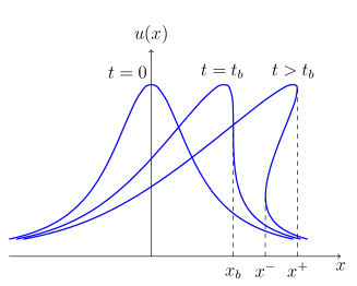
Figure 1: Evolution of a typical pulse in accordance with Hopf equation (10). After the instant of breaking, $t>t_{b}$, the distribution $u(x,t)$ formally becomes a three-valued function of the coordinate $x$ in the domain $x^{-}<x<x^{+}$.

With dispersion ignored, Eq. (9) becomes the Hopf equation

$$u_{t}+6uu_{x}=0,$$ (10)

which is a dimensionless form of Eq. (7). It readily follows that $u$ is constant along the characteristics $x-6ut=\mathrm{const}$, which are solutions of the equation $dx/dt=6u$. Therefore, if the initial distribution $u$ is described by a function $u=u_{0}(x)$ at $t=0$ and $x=\overline{x}(u)$ is the inverse function, then the implicit solution of the Hopf equation is given by

$$x-6ut=\overline{x}(u),$$ (11)

which describes the distribution $u(x,t)$ at subsequent times.

The most significant feature of these solutions is that the transfer speed of $u$ values increases as $u$ increases and, for typical initial distributions $u_{0}(x)$, the solution becomes multi-valued after a certain instant $t=t_{b}$, as is shown in Fig. 1. Evidently, we have gone outside the applicability domain of the dispersionless approximation: at the instant of breaking $t=t_{b}$, the derivative of the distribution with respect to $x$ becomes infinitely large at the point $x_{b}$, and the dispersion term with the third-order derivative in KdV equation (9) is by no means small in the vicinity of $x_{b}$. As noted in the Introduction, taking dispersion into account suppresses this nonphysical behavior, and in the solution of the full KdV equation the multi-valuedness domain is superseded with an oscillatory domain evolving with time, i.e., a dispersive shock wave. Gurevich and Pitaevskii assumed that this oscillatory domain can be approximately represented as a modulated periodic solution of the KdV equation, which means that the next step in constructing the DSW theory must consist of deriving such periodic solutions—which was done by Korteweg and de Vries themselves in kdv . Here, we give the necessary background. As usual, we seek a solution of Eq. (9) as a traveling wave $u=u(\xi)$, $\xi=x-Vt$, where $V$ is the wave propagation speed; we then find that $u(\xi)$ satisfies the ordinary differential equation $u_{\xi\xi\xi}=Vu_{\xi}-6uu_{\xi}$, which, after two elementary integrations, takes the form of the equation

$$\begin{split}\tfrac{1}{2}u_{\xi}^{2}&=-A+Bu+\tfrac{1}{2}Vu^{2}-u^{3}=\\ &=-\mathcal{R}(u)=-(u-\nu_{1})(u-\nu_{2})(u-\nu_{3}),\end{split}$$ (12)

where $A$ and $B$ are constants of integration. This equation has real solutions if the polynomial $\mathcal{R}(u)$ has three real zeros: $\nu_{1}$, $\nu_{2}$, and $\nu_{3}$ with $\nu_{1}\leq\nu_{2}\leq\nu_{3}$. Evidently, the oscillating solution corresponds to the motion of $u$ between two zeros in the interval

$$\nu_{2}\leq u\leq\nu_{3},$$ (13)

where $\mathcal{R}(u)\leq 0$. The constants $A$, $B$, and $V$ can be expressed in terms of $\nu_{1}$, $\nu_{2}$, and $\nu_{3}$ as

$$\begin{split}&A=-\nu_{1}\nu_{2}\nu_{3},\quad B=-(\nu_{1}\nu_{2}+\nu_{2}\nu_{3}+\nu_{3}\nu_{1}),\\ &V=2(\nu_{1}+\nu_{2}+\nu_{3}).\end{split}$$ (14)

It now follows from Eq. (12) that the periodic solution of the KdV equation can be expressed as

$$\sqrt{2}\,\xi=\int\limits_{u}^{\nu_{3}}\frac{du^{\prime}}{\sqrt{(u^{\prime}-\nu_{1})(u^{\prime}-\nu_{2})(\nu_{3}-u^{\prime})}},$$ (15)

where the integration constant that is additive with respect to $\xi$ is chosen such that $u(\xi)$ takes the maximum value $\nu_{3}$ at $\xi=0$. Integral (15) can be standardly expressed in terms of elliptic integrals, and their inversion gives the dependence $u=u(\xi)$ in terms of elliptic functions. Omitting the calculations that are routine for nonlinear physics, we get the result

$$u=\nu_{3}-(\nu_{3}-\nu_{2})\,\mathrm{sn}^{2}\left(\sqrt{({\nu_{3}-\nu_{1}})/{2}}\,(x-Vt),m\right),$$ (16)

where $\mathrm{sn}$ is the elliptic sine, and the parameter $m$ is defined as

$$m=\frac{\nu_{3}-\nu_{2}}{\nu_{3}-\nu_{1}}$$ (17)

in accordance with the notation in handbook AS-2 . Using the identity $\mathrm{sn}^{2}z+\mathrm{cn}^{2}z=1$ allows expressing this solution in terms of the elliptic cosine $\mathrm{cn}$, which is why Korteweg and de Vries called their solution the ‘cnoidal wave’, similarly to the cosine wave in the linear theory. The properties of such a cnoidal wave are determined by the three zeros, $\nu_{1},\nu_{2},$ and $\nu_{3}$, of the polynomial $\mathcal{R}(u)$. In particular, the speed of the wave $V$ and the parameter $m$ are expressed by formulas (14) and (17). The wavelength $L$ can be defined as the distance between two neighboring maxima of $u(\xi)$, and it is then expressed through the full elliptic integral of the first kind $K(m)$ as

$$L=\oint\frac{du}{\sqrt{-2\mathcal{R}(u)}}=\frac{2\sqrt{2}K(m)}{\sqrt{\nu_{3}-\nu_{1}}}$$ (18)

The cnoidal wave amplitude can be defined by the relation

$$a=(u_{max}-u_{min})/2=(\nu_{3}-\nu_{2})/2.$$ (19)

Solution (16) passes into a harmonic linear-approximation wave

$$u\cong\nu_{2}+\frac{1}{2}(\nu_{3}-\nu_{2})\cos\left(\sqrt{2(\nu_{2}-\nu_{1})}(x-Vt)\right).$$ (20)

for a small wave amplitude $a\ll\nu_{2}-\nu_{1}$, when $m\ll 1$. The wave number $k=2\pi/L=\sqrt{2(\nu_{2}-\nu_{1})}$ and the phase velocity $V=2\nu_{1}+4\nu_{2}=6\nu_{2}-k^{2}$ of the wave are then related as $V=\omega/k$, which follows from the dispersion law $\omega=6\nu_{2}k-k^{3}$ that corresponds to the linearized KdV equation $u^{\prime}_{t}+6\nu_{2}u^{\prime}_{x}+u^{\prime}_{xxx}=0$ for a wave propagating along the uniform state with $u=\nu_{2}$.

In the opposite limit $\nu_{2}\to\nu_{1}$ and $m\to 1$, the wavelength tends to infinity and $\mathrm{sn}(z,1)=\th(z)$, and hence solution (16) becomes

$$u=\nu_{1}+\frac{\nu_{3}-\nu_{1}}{\ch^{2}\left(\sqrt{(\nu_{3}-\nu_{1})/2}\,(x-Vt)\right)}.$$ (21)

In this case, the profile $u=u(x-Vt)$ has the shape of a solitary wave propagating along the uniform state $u=\nu_{1}$. Thus, in the limit $m\to 1$, the periodic wave transforms into solitary pulses, or solitons (21), separated by an infinitely long distance.

The fundamental assumption of Gurevich and Pitaevskii’s approach to the DSW theory was that at sufficiently large times after the instant of breaking, when the length of the emerging oscillatory domain becomes much greater than the local wavelengths $L$, the DSW evolution can be represented as a slow variation of the parameters $\nu_{1},\nu_{2}$, and $\nu_{3}$ in a modulated cnoidal wave (16). The ‘slowness’ condition here means that the relative change in the modulation parameters $\nu_{1},\nu_{2}$, and $\nu_{3}$ or the equivalent variables is small either at distances of the order of the wavelength $L$ or over a time of the order of one oscillation period.

Thus, the problem of constructing the theory of DSWs reduces to deriving equations for the evolution of modulation parameters and to obtaining their solutions in specific physical situations. Fortunately, by that time, equations for the modulation of a cnoidal KdV wave had already been derived by Whitham whitham-65 . Unfortunately, in both  whitham-65 and his later book whitham-74 , Whitham only gave the final result of the calculations, having omitted all the details. Because these calculations are highly nontrivial, we briefly describe them in Section 4 for completeness, but first, with methodological purposes in mind, we discuss a linear-approximation analogue of Whitham’s modulation theory.

3 Modulation of linear waves

A well-known result in the theory of modulation of linear waves is that the envelope of a modulated wave packet propagates with the group velocity of the carrier wave. Methods for deriving asymptotic solutions of linear equations have also been developed in much detail to describe such behavior of waves. But we look at problems of this sort from another standpoint, which is very transparent physically and allows an extension to the dynamics of nonlinear waves.

As an example, we consider the evolution of a wave described by the linearized KdV equation $u^{\prime}_{t}+6\nu_{2}u^{\prime}_{x}+u^{\prime}_{xxx}=0$ and having the initial shape of a ‘step’. Because the $6\nu_{2}u^{\prime}_{x}$ can easily be eliminated by passing to the reference frame $x^{\prime}=x-6\nu_{2}t,t^{\prime}=t$, we write the linear KdV equation as

$$u_{t}+u_{xxx}=0,$$ (22)

and take the initial condition in the form

$$u_{0}(x)=\begin{cases}1,&\text{ $x\leq 0$},\\ 0,&\text{ $x>0$.}\end{cases}$$ (23)

This problem can easily be solved exactly by the Fourier method, and the result can be brought to the form

$$u(x,t)=\int\limits_{x/(3t)^{1/3}}^{\infty}\mathrm{Ai}(z)\,dz,$$ (24)

where $\mathrm{Ai}(z)$ is the standard notation for the Airy function AS-2 . As we can see, the wave profile depends only on the self-similar variable $z={x}/{(3t)^{1/3}}$ (Fig. 2). At large $x$, when $z\gg 1$, the wave amplitude decreases exponentially into the ‘shadow’ domain, and in the opposite limit of large negative $x$, we can use the known asymptotic form of the Airy function to obtain ($-z\gg 1$)

$$u(z)\cong 1-\frac{1}{\sqrt{\pi}}(-z)^{-3/4}\cos\left(\tfrac{2}{3}(-z)^{3/2}+\tfrac{\pi}{4}\right).$$ (25)

The obtained results confirm the general idea that dispersive effects manifest themselves in oscillatory wave structures originating from pulses with sufficiently sharp fronts. But the shape of the resultant wave structure suggests another approach to its description.

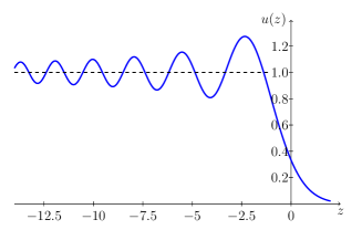
Figure 2: Profile of wave (24) plotted as a function of the self-similar variable $z=x/(3t)^{1/3}$.

Both Fig. 2 and formula (25) suggest that, as $x\to-\infty$, this wave can be interpreted as a modulated harmonic wave with a variable wave number and variable frequency and amplitude of oscillations. We represent such a wave as

$$u(x,t)=1+a(x,t)\cos[\theta(x,t)+\theta_{0}],$$ (26)

where we introduce the wave phase

$$\theta(x,t)=\frac{2}{3}\left(\frac{-x}{(3t)^{1/3}}\right)^{3/2},$$ (27)

having for simplicity dropped the constant term $\theta_{0}=\pi/4$ from its definition. For such a modulated wave, it is natural to define the wave number $k(x,t)$ and the frequency $\omega(x,t)$ as

$$\begin{split}&k(x,t)=\theta_{x}(x,t)=-\left(\frac{-x}{3t}\right)^{1/2},\\ &\omega(x,t)=-\theta_{t}(x,t)=\left(\frac{-x}{3t}\right)^{3/2},\end{split}$$ (28)

which are locally related by the dispersion law $\omega=-k^{3}$ that follows from linear KdV equation (22). In other words, wave (26) is locally a harmonic wave that is an exact solution of this equation if modulation is ignored. If we consider a piece of the structure with a fixed wave number $k(x,t)$, it immediately follows from the first formula in (28) that this piece moves along the $x$ axis with the group velocity

$$v_{g}=-3k^{2}=\frac{d\omega}{dk}$$ (29)

in accordance with the known property of the group velocity. It is clear that this way of introducing the group velocity into the theory of modulation of linear waves has a general character.

We assume that the modulated linear wave is represented as

$$u(x,t)=a(x,t)\cos[\theta(x,t)],$$ (30)

and that this wave is locally harmonic with good accuracy, with local values of the wave number and frequency defined as

$$k(x,t)=\theta_{x}(x,t),\qquad\omega(x,t)=-\theta_{t}(x,t),$$ (31)

and related by the dispersion law for harmonic waves

$$\omega=\omega(k).$$ (32)

In view of (31), the consistency condition for cross derivatives of the phase $(\theta_{x})_{t}=(\theta_{t})_{x}$ leads to the equation

$$k_{t}+\omega_{x}=0\quad\text{или}\quad k_{t}+(kV)_{x}=0,$$ (33)

where $V=V(k)$ is the phase velocity of the wave. Because a unit-length interval along the $x$ axis contains $1/L=k/(2\pi)$ waves, Eq. (33) can be interpreted as the conservation law for the number of waves, with $k$ playing the role of the density of waves and $\omega=kV$ the flux. Substituting dispersion law (33) into (32), we arrive at the equation

$$k_{t}+v_{g}(k)k_{x}=0,$$ (34)

which again states that the wave number $k$ propagates at the speed $v_{g}(k)=\omega^{\prime}(k)$ and preserves its value along the characteristic $x-v_{g}(k)t=\mathrm{const}$. Therefore, if changes in the shape of the wave packet are disregarded, a wave packet made of harmonics with the wave numbers close to $k=k_{0}$ propagates with the group velocity $v_{g}(k_{0})=\omega^{\prime}(k_{0})$.

We can now return to the problem of the decay of a step-like profile with initial distribution (23) and use Eq. (34) instead of the exact solution expressed in terms of the Airy function. The key role here is played by the observation that the initial distribution does not contain parameters with the dimension of length, but the original problem has some characteristic value of speed $c_{0}$. Therefore, a solution of Eq. (34) can depend only on the self-similar variable $\xi=x/t$ (in dimensional units, on $\xi=x/(c_{0}t)$). Substituting $k=k(\xi)$ into (34), we find $(dk/d\xi)(v_{g}(k)-\xi)=0$. Because $dk/d\xi\neq 0$ along the modulated wave, the dependence $k=k(\xi)$ is defined implicitly by the equation

$$v_{g}(k)=\xi=\frac{x}{t}.$$ (35)

Having used this to find $k=k(x/t)$, we can express the phase $\theta(x,t)$ from the equation $\theta_{x}=k$ if we recall that the frequency $\omega=-\theta_{t}$, which is a function of $k$, can also depend only on the self-similar variable. For the linear KdV equation, the obtained results immediately reproduce the known relations $-3k^{2}={x}/t$, $k=\theta_{x}=-(-x/(3t))^{1/2}$, $\theta=\frac{2}{3}({-x}/{(3t)^{1/3}})^{3/2}$. Thus, modulation equation (34) has allowed us to easily find some characteristics of the emergent wave structure.

To derive the modulation equation for the amplitude $a(x,t)$ of wave (30), it is natural to use the energy conservation law, because expansion of the wave structure with time leads to a redistribution of energy over a progressively larger volume, and in linear systems the energy density is proportional to the amplitude squared. After averaging over the wavelength, the local energy density $a^{2}(x,t)$ is transported with the group velocity $v_{g}$ corresponding to the local value of the wave number $k$, and we can therefore write the energy conservation law as

$$\frac{\partial(a^{2})}{\partial t}+\frac{\partial(v_{g}a^{2})}{\partial x}=0.$$ (36)

In the case of a linear KdV equation and asymptotic regime (35) of the wave packet evolution, Eq. (36) becomes $ta_{t}+xa_{x}=-\frac{1}{2}a$. This can readily be solved using the standard method of characteristics, with the result $a(x,t)=(1/{\sqrt{t}})f({x}/t)$, where $f$ is an arbitrary function. Assuming that in the problem of the evolution of a step-like shape the amplitude also depends only on the same self-similar variable $z={-x}/{(3t)^{1/3}}$ as the wave number $k$ does, it is easy to find that $f(x/t)=\mathrm{const}\cdot(-x/t)^{-3/4}$, which defines the modulated wave shape up to a constant factor:

$$u(x,t)\cong\frac{\mathrm{const}}{\sqrt{t}}\left(\frac{-x}{t}\right)^{-3/4}\cos\left[\frac{2}{3}\frac{(-x)^{3/2}}{(3t)^{1/2}}\right].$$

Thus, we have reproduced the main features of solution (25) without relying on any information on the properties of the Airy function, but rather by just solving modulation equations (34) and (36) of the linear theory. Evidently, the idea of this approach involving the wave number conservation law and other conservation laws with averaged densities and fluxes allows a generalization to nonlinear waves. Exactly that was done by Whitham for modulated cnoidal waves of the KdV equation, and we discuss his theory in Section 4.

4 Whitham theory

We restrict ourselves to describing the general idea of Whitham whitham-65 on averaging conservation laws in the simple case where the evolution of a wave is described by a nonlinear equation for a single variable $u$,

$$\Phi(u,u_{t},u_{x},u_{tt},u_{tx},u_{xx},\ldots)=0.$$ (37)

We assume that Eq. (37) has traveling-wave solutions when $u(x,t)$ depends on $x$ and $t$ only through the combination $u=u(\xi)$, $\xi=x-Vt$, and for such solutions, Eq. (37) can be reduced to the form

$$u_{\xi}^{2}=F(u,V,A_{i}),$$ (38)

where $A_{i}$ is a collection of parameters occurring in deriving (38) from (37). In a periodic traveling wave, the variable $u$ oscillates between two zeros of $F(u)$. We let $u_{1}(V,A_{i})$ and $u_{2}(V,A_{i})$, with $u_{1}<u_{2}$, denote these zeros, assuming that $F$ is positive in the interval $u_{1}<u<u_{2}$. Obviously, the wavelength is

$$L=L(V,A_{i})=2\int_{u_{1}}^{u_{2}}\frac{du}{\sqrt{F(u;V,A_{i})}},$$ (39)

and the wave number $k$ and the frequency $\omega$ are

$$\begin{split}&k=k(V,A_{i})=1/L(V,A_{i}),\\ &\omega=\omega(V,A_{i})=Vk(V,A_{i}),\end{split}$$ (40)

where we dropped the factor $2\pi$ in the definition of the wave number because it is only needed in the nonlinear theory for maintaining correspondence with the low-amplitude limit, and this factor can easily be restored whenever necessary. As a result, the wave number $k$ becomes exactly equal to the density of the number of waves. In a modulated wave $u(\xi;V,A_{i})$, the parameters $V$ and $A_{i}$ are slowly varying functions of $x$ and $t$, changing little over distances of the order of the wavelength $L$ and over a time of the order of $1/\omega$. This implies that there is an interval $\Delta$, much longer than the wavelength $L$ but much shorter than a certain size $l$ characterizing the wave structure overall: $L\ll\Delta\ll l$. It is clear that, up to small quantities of the order of $\varepsilon\sim\Delta/l$, averaging over the interval $\Delta$ is equivalent to averaging over the wavelength $L$. Therefore, we average physical quantities over fast oscillations in the wave in accordance with the rule

$$\langle\mathcal{F}\rangle\approx\frac{1}{L}\int_{0}^{L}\mathcal{F}(x^{\prime},t)dx^{\prime}.$$ (41)

If a conservation law $\mathcal{P}_{t}+\mathcal{Q}_{x}=0$ is known, then, after the averaging, it takes the form

$$\frac{\partial}{\partial t}\langle\mathcal{P}\rangle+\frac{\partial}{\partial x}\langle\mathcal{Q}\rangle=0,$$ (42)

where the dependence on $x$ and $t$ is only present in slowly varying modulation parameters $V$ and $A_{i}$ that enter the averaged quantities. We can regard Eqs (42) as differential equations for these parameters, similarly to how we viewed modulation equations in the linear theory.

We can now turn to the derivation of the modulation equations for the cnoidal KdV wave. In a weakly modulated wave, the parameters $A,\,B,\,V$ or $\nu_{1},\,\nu_{2},\,\nu_{3}$ become slowly varying functions of $x$ and $t$, and we wish to find the equations governing the evolution of these parameters. Calculations can be simplified by recalling that one of the modulation equations is already known. Replacing the elliptic function argument in periodic solution (16) with the phase $\theta$ that can be defined up to an appropriate numerical factor, we introduce local values of the wave number and frequency via formulas (31), just as in the linear case; they must then satisfy the conservation law for the number of waves in Eq. (33). In a weakly modulated wave, the values of $k$ and $\omega$ are given by Eqs. (40) with variable parameters $V$ and $A_{i}$, and hence variations of these parameters under the evolution of the wave must satisfy the equation

$$k_{t}+(kV)_{x}=0,\qquad k=1/L.$$ (43)

As two missing modulation equations, we use the averaged conservation laws:

$$\begin{split}&u_{t}+(3u^{2}+u_{xx})_{x}=0,\\ &(\tfrac{1}{2}u^{2})_{t}+(2u^{3}+uu_{xx}-\tfrac{1}{2}u_{x}^{2})_{x}=0,\\ \end{split}$$ (44)

which can be straightforwardly verified by substituting $u_{t}$ from the KdV equation.

We first derive the modulation equations for the para- meters $A,\,B$, and $V$. Following Whitham, we express the averaged quantities in terms of the function

$$\begin{split}\mathcal{W}&=-\sqrt{2}\oint\sqrt{-A+Bu+\tfrac{1}{2}Vu^{2}-u^{3}}\,\,du=\\ &=-\sqrt{2}\oint\sqrt{-\mathcal{R}(u)}\,du,\end{split}$$ (45)

where the integral is taken over a closed contour encompassing the interval $\nu_{2}\leq u\leq\nu_{3}$. The wavelength $L=1/k$ is then expressed through $\mathcal{W}$ as

$$L=\frac{1}{\sqrt{2}}\oint\frac{du}{\sqrt{-\mathcal{R}(u)}}=\frac{\partial\mathcal{W}}{\partial A}\equiv\mathcal{W}_{A}.$$ (46)

We readily calculate the averaged quantities:

$$\begin{split}&\langle u\rangle=k\int_{0}^{L}u\,d\xi=\frac{k}{\sqrt{2}}\oint\frac{u\,du}{\sqrt{-\mathcal{R}(u)}}=-k\mathcal{W}_{B},\\ &\langle\tfrac{1}{2}u^{2}\rangle=k\int_{0}^{L}\frac{\tfrac{1}{2}u^{2}du}{u_{\xi}}=-k\mathcal{W}_{V},\\ &\langle u_{\xi}^{2}\rangle=k\oint\frac{u_{\xi}^{2}du}{u_{\xi}}=-k\mathcal{W}.\end{split}$$ (47)

The second derivatives $u_{\xi\xi}$ can be eliminated from the conservation laws with the help of the formula $u_{\xi\xi}=B+Vu-3u^{2}$. After simple calculations using the relation $k\mathcal{W}_{A}=1$ and the averaged values found above, we obtain the averaged conservation laws:

$$\begin{split}(k\mathcal{W}_{B})_{t}&+(kV\mathcal{W}_{B}-B)_{x}=0,\\ (k\mathcal{W}_{V})_{t}&+(kV\mathcal{W}_{V}-A)_{x}=0,\\ \end{split}$$ (48)

Having substituted $k=1/\mathcal{W}_{A}$ and introduced the ‘long’ derivative $D/Dt=\partial/\partial t+V\partial/\partial x$, we obtain the modulation equations

$$\begin{split}&\frac{D\mathcal{W}_{A}}{Dt}=\mathcal{W}_{A}\frac{\partial V}{\partial x},\quad\frac{D\mathcal{W}_{B}}{Dt}=\mathcal{W}_{A}\frac{\partial B}{\partial x},\\ &\frac{D\mathcal{W}_{V}}{Dt}=\mathcal{W}_{A}\frac{\partial A}{\partial x},\end{split}$$ (49)

the first of which is the conservation law (43) with the wave number expressed as $k=1/\mathcal{W}_{A}$.

Despite the apparent simplicity of the obtained equations, they are not extremely useful in practice. We therefore reexpress them in terms of $\nu_{1},\,\nu_{2}$, and $\nu_{3}$. From (14), we find the relations between differentials:

$$\begin{split}&dV=2(d\nu_{1}+d\nu_{2}+d\nu_{3}),\\ &dB=-[(\nu_{2}+\nu_{3})d\nu_{1}+(\nu_{1}+\nu_{3})d\nu_{2}+(\nu_{1}+\nu_{2})d\nu_{3}],\\ &dA=-(\nu_{2}\nu_{3}\cdot d\nu_{1}+\nu_{1}\nu_{3}\cdot d\nu_{2}+\nu_{1}\nu_{2}\cdot d\nu_{3}).\end{split}$$

Hence, Eqs. (49) expressed in the variables $\nu_{1},\,\nu_{2}$, and $\nu_{3}$ take the form

$$\begin{split}&\mathcal{W}_{A,\nu_{1}}\frac{D\nu_{1}}{Dt}+\mathcal{W}_{A,\nu_{2}}\frac{D\nu_{2}}{Dt}+\mathcal{W}_{A,\nu_{3}}\frac{D\nu_{3}}{Dt}=\\ &=2\mathcal{W}_{A}(\nu_{1,x}+\nu_{2,x}+\nu_{3,x}),\\ &\mathcal{W}_{B,\nu_{1}}\frac{D\nu_{1}}{Dt}+\mathcal{W}_{B,\nu_{2}}\frac{D\nu_{2}}{Dt}+\mathcal{W}_{B,\nu_{3}}\frac{D\nu_{3}}{Dt}=\\ &=-\mathcal{W}_{A}[(\nu_{2}+\nu_{3})\nu_{1,x}+(\nu_{1}+\nu_{3})\nu_{2,x}+(\nu_{1}+\nu_{2})\nu_{3,x}],\\ &\mathcal{W}_{V,\nu_{1}}\frac{D\nu_{1}}{Dt}+\mathcal{W}_{V,\nu_{2}}\frac{D\nu_{2}}{Dt}+\mathcal{W}_{V,\nu_{3}}\frac{D\nu_{3}}{Dt}=\\ &=-\mathcal{W}_{A}[\nu_{2}\nu_{3}\cdot\nu_{1,x}+\nu_{1}\nu_{3}\cdot\nu_{2,x}+\nu_{1}\nu_{2}\cdot\nu_{3,x}],\end{split}$$ (50)

where all the derivatives of$\mathcal{W}$ are represented by integrals similar to (45) and (47).

As a clue to further transformations, we note that the right-hand sides of Eqs. (50) contain the same factor $\mathcal{W}_{A}$. Therefore, their linear combinations can be found such that the coefficient in front of one of the derivatives vanishes and the other two coefficients become equal. Indeed, we multiply the first equation in (50) by $p$, the second by $q$, and the third by $r$, add them, and choose the parameters $p,q$, and $r$ such that the coefficient in front of $\nu_{1,x}$ vanishes and the coefficients in front of $\nu_{2,x}$ and $\nu_{3,x}$ become equal:

$$\begin{split}&2p-q(\nu_{2}+\nu_{3})-r\nu_{2}\nu_{3}=0,\\ &2p-q(\nu_{1}+\nu_{3})-r\nu_{1}\nu_{3}=2p-q(\nu_{1}+\nu_{2})-r\nu_{1}\nu_{2}.\end{split}$$

It immediately follows from these conditions that

$$q=-r\nu_{1},\qquad p=-\frac{1}{2}r(\nu_{1}\nu_{2}+\nu_{1}\nu_{3}-\nu_{2}\nu_{3})$$

and we can hence set $r=-2$, to obtain $p=\nu_{1}\nu_{2}+\nu_{1}\nu_{3}-\nu_{2}\nu_{3}$, $q=2\nu_{1}$, and $r=-2$. The right-hand side of this linear combination of Eqs. (50) then takes the form

$$-2(\nu_{2}-\nu_{1})(\nu_{3}-\nu_{1})\mathcal{W}_{A}\frac{\partial(\nu_{2}+\nu_{3})}{\partial x}.$$ (51)

Hence, it follows that, if in a similar linear combination of the left-hand sides of Eqs. (50) the coefficient in front of ${D\nu_{1}}/{Dt}$ vanishes and the coefficient in front of ${D\nu_{2}}/{Dt}$ and ${D\nu_{3}}/{Dt}$ are equal to each other, then the modulation equations take a very simple ‘diagonal’ form.

With the help of the identity

$$\begin{split}&\frac{d}{du}\left(2\sqrt{\frac{(u-\nu_{2})(u-\nu_{3})}{-(u-\nu_{1})}}\right)=\\ &=-\frac{u^{2}-2\nu_{1}u+\nu_{1}\nu_{2}+\nu_{1}\nu_{3}-\nu_{2}\nu_{3}}{(u-\nu_{1})\sqrt{-\mathcal{R}(u)}}\end{split}$$

which is easy to verify, we obtain

$$\begin{split}&p\mathcal{W}_{A,\nu_{1}}+q\mathcal{W}_{B,\nu_{1}}+r\mathcal{W}_{V,\nu_{1}}=\\ &=-\frac{1}{\sqrt{8}}\oint\frac{d}{du}\left(2\sqrt{\frac{(u-\nu_{2})(u-\nu_{3})}{-(u-\nu_{1})}}\right)du=0,\end{split}$$

because the integrand is a total derivative of a periodic function, and the first condition is thus satisfied.

The coefficients in front of ${D\nu_{2}}/{Dt}$ and ${D\nu_{3}}/{Dt}$ have the respective forms

$$\begin{split}&K_{2}=p\mathcal{W}_{A,\nu_{2}}+q\mathcal{W}_{B,\nu_{2}}+r\mathcal{W}_{V,\nu_{2}}=\\ &=\frac{1}{\sqrt{8}}\oint\frac{u^{2}-2\nu_{1}u+\nu_{1}\nu_{2}+\nu_{1}\nu_{3}-\nu_{2}\nu_{3}}{(u-\nu_{2})\sqrt{-\mathcal{R}(u)}}du,\\ &K_{3}=p\mathcal{W}_{A,\nu_{3}}+q\mathcal{W}_{B,\nu_{3}}+r\mathcal{W}_{V,\nu_{3}}=\\ &=\frac{1}{\sqrt{8}}\oint\frac{u^{2}-2\nu_{1}u+\nu_{1}\nu_{2}+\nu_{1}\nu_{3}-\nu_{2}\nu_{3}}{(u-\nu_{3})\sqrt{-\mathcal{R}(u)}}du,\end{split}$$

and their difference, being an integral of the derivative of a periodic function over the period, vanishes:

$$\begin{split}&K_{2}-K_{3}=\\ &=\frac{\nu_{2}-\nu_{3}}{\sqrt{8}}\oint\frac{d}{du}\left(2\sqrt{\frac{-(u-\nu_{1})}{(u-\nu_{2})(u-\nu_{3})}}\right)du=0.\end{split}$$

Hence, $K_{2}=K_{3}$, and the combination $\nu_{2}+\nu_{3}$ is a convenient modulation variable for which the modulation equations are dramatically simplified. The emerging coefficient $K_{2}=K_{3}$ in front of $D(\nu_{2}+\nu_{3})/Dt$ can also be expressed in terms of $\mathcal{W}_{A}$. Indeed, $K_{2}$ and $K_{3}$ can be represented as

$$\begin{split}&K_{2}=\frac{\nu_{2}-\nu_{1}}{\sqrt{2}}\oint\frac{(u-\nu_{3})du}{(u-\nu_{2})\sqrt{-\mathcal{R}(u)}}+\\ &+\frac{1}{\sqrt{8}}\oint\frac{u^{2}-2\nu_{2}u+\nu_{1}\nu_{2}+\nu_{2}\nu_{3}-\nu_{1}\nu_{3}}{(u-\nu_{2})\sqrt{-\mathcal{R}(u)}}du,\\ &K_{3}=\frac{\nu_{3}-\nu_{1}}{\sqrt{2}}\oint\frac{(u-\nu_{2})du}{(u-\nu_{3})\sqrt{-\mathcal{R}(u)}}+\\ &+\frac{1}{\sqrt{8}}\oint\frac{u^{2}-2\nu_{3}u+\nu_{1}\nu_{3}+\nu_{2}\nu_{3}-\nu_{1}\nu_{2}}{(u-\nu_{3})\sqrt{-\mathcal{R}(u)}}du.\end{split}$$

But the second terms on the right-hand sides vanish due to identities quite similar to those used above, and the remaining non-vanishing terms can be easily brought to the form

$$\begin{split}&K_{2}=(\nu_{2}-\nu_{1})\mathcal{W}_{A}-2(\nu_{2}-\nu_{1})(\nu_{3}-\nu_{2})\mathcal{W}_{A,\nu_{2}},\\ &K_{3}=(\nu_{3}-\nu_{1})\mathcal{W}_{A}+2(\nu_{3}-\nu_{1})(\nu_{3}-\nu_{2})\mathcal{W}_{A,\nu_{3}}.\end{split}$$ (52)

The equality $K_{2}=K_{3}$ then leads to the identity

$$\mathcal{W}_{A}=-2[(\nu_{2}-\nu_{1})\mathcal{W}_{A,\nu_{2}}+(\nu_{3}-\nu_{1})\mathcal{W}_{A,\nu_{3}}],$$

substituting which in any of the equations in (52) gives

$$\begin{split}K_{2}=K_{3}&=-2(\nu_{2}-\nu_{1})(\nu_{3}-\nu_{1})(\mathcal{W}_{A,\nu_{2}}+\mathcal{W}_{A,\nu_{3}})=\\ &=2(\nu_{2}-\nu_{1})(\nu_{3}-\nu_{1})\mathcal{W}_{A,\nu_{1}},\end{split}$$

because

$$\mathcal{W}_{A,\nu_{1}}+\mathcal{W}_{A,\nu_{2}}+\mathcal{W}_{A,\nu_{3}}=\frac{1}{\sqrt{8}}\oint\frac{-\mathcal{R}^{\prime}(u)du}{(-\mathcal{R})^{3/2}(u)}=0.$$

We now equate the left-hand side of our linear combination

$$2(\nu_{1}-\nu_{2})(\nu_{1}-\nu_{3})\mathcal{W}_{A,\nu_{1}}\frac{D(\nu_{2}+\nu_{3})}{Dt},$$

to its right-hand side in (51) to obtain the equation

$$\frac{D(\nu_{2}+\nu_{3})}{Dt}+\frac{\mathcal{W}_{A}}{\mathcal{W}_{A,\nu_{1}}}\frac{\partial(\nu_{2}+\nu_{3})}{\partial x}=0.$$ (53)

Cyclic permutations of $\nu_{1},\,\nu_{2}$, and $\nu_{3}$ give two other Whitham modulation equations:

$$\begin{split}&\frac{D(\nu_{3}+\nu_{1})}{Dt}+\frac{\mathcal{W}_{A}}{\mathcal{W}_{A,\nu_{2}}}\frac{\partial(\nu_{3}+\nu_{1})}{\partial x}=0,\\ &\frac{D(\nu_{1}+\nu_{2})}{Dt}+\frac{\mathcal{W}_{A}}{\mathcal{W}_{A,\nu_{3}}}\frac{\partial(\nu_{1}+\nu_{2})}{\partial x}=0.\end{split}$$ (54)

Each of the equations obtained by Whitham involve derivatives of only one of the quantities $\nu_{2}+\nu_{3}$, $\nu_{3}+\nu_{1}$, and $\nu_{1}+\nu_{2}$, which means that the equations have acquired a diagonal form. Therefore, the above transformation is similar to the transition from the standard form of gas-dynamic equations to their diagonal form in terms of different variables, called Riemann invariants (see, e.g., LL6 ). We therefore define the new modulation variables, the Riemann invariants $r_{1}\leq r_{2}\leq r_{3}$ of Whitham modulation equations, as

$$\begin{split}&r_{1}=\tfrac{1}{2}(\nu_{1}+\nu_{2}),\quad r_{2}=\tfrac{1}{2}(\nu_{1}+\nu_{3}),\\ &r_{3}=\tfrac{1}{2}(\nu_{2}+\nu_{3});\\ &\nu_{1}=r_{1}+r_{2}-r_{3},\quad\nu_{2}=r_{1}+r_{3}-r_{2},\\ &\nu_{3}=r_{2}+r_{3}-r_{1},\end{split}$$ (55)

and express the other variables through them. In particular, we find $\mathcal{W}_{A,r_{1}}=\mathcal{W}_{A,\nu_{1}}+\mathcal{W}_{A,\nu_{2}}-\mathcal{W}_{A,\nu_{3}}=-2\mathcal{W}_{A,\nu_{3}}$, $\mathcal{W}_{A,r_{2}}=-2\mathcal{W}_{A,\nu_{2}}$, and $\mathcal{W}_{A,r_{3}}=-2\mathcal{W}_{A,\nu_{1}}$. With $\mathcal{W}_{A}=L$, we obtain

$$\frac{\mathcal{W}_{A}}{\mathcal{W}_{A,\nu_{1}}}=-\frac{2\mathcal{W}_{A}}{\mathcal{W}_{A,r_{3}}}=-\frac{2L}{\partial L/\partial r_{3}},$$

and similar formulas for $\mathcal{W}_{A}/\mathcal{W}_{A,\nu_{2}}$ and $\mathcal{W}_{A}/\mathcal{W}_{A,\nu_{3}}$. Finally, because

$$V=2(\nu_{1}+\nu_{2}+\nu_{3})=2(r_{1}+r_{2}+r_{3}),$$ (56)

we can represent Whitham equations as

$$\frac{\partial r_{i}}{\partial t}+v_{i}(r_{1},r_{2},r_{3})\frac{\partial r_{i}}{\partial x}=0,\quad i=1,2,3,$$ (57)

with the characteristic velocities

$$\begin{split}v_{i}&=2(r_{1}+r_{2}+r_{3})-\frac{2L}{\partial L/\partial r_{i}}=\\ &=\left(1-\frac{L}{\partial_{i}L}\partial_{i}\right)V,\quad i=1,2,3,\end{split}$$ (58)

where $\partial_{i}\equiv\partial/\partial r_{i}$. Because formula (18) for the wavelength becomes

$$L=\frac{2K(m)}{\sqrt{r_{3}-r_{1}}},\quad m=\frac{r_{2}-r_{1}}{r_{3}-r_{1}},$$ (59)

substitution of (59) into (58) using the known expression for the derivative of the elliptic integral $K(m)$ (see, e.g., AS-2 ) allows expressing the velocities $v_{i}$ as

$$\begin{split}&v_{1}=2(r_{1}+r_{2}+r_{3})+\frac{4(r_{2}-r_{1})K(m)}{E(m)-K(m)},\\ &v_{2}=2(r_{1}+r_{2}+r_{3})-\frac{4(r_{2}-r_{1})(1-m)K(m)}{E(m)-(1-m)K(m)},\\ &v_{3}=2(r_{1}+r_{2}+r_{3})+\frac{4(r_{3}-r_{1})(1-m)K(m)}{E(m)},\end{split}$$ (60)

where $E(m)$ is the full elliptic integral of the second kind. This is just the form of modulation equations for cnoidal KdV waves arrived at by Whitham in whitham-65 .

The possibility of transforming a system of three first-order equations to diagonal form is a highly nontrivial fact. Fortunately, Whitham was unaware of a theorem stating that such a transformation is in general impossible in systems of more than two equations (see, e.g., rozhd-yan ). In whitham-74 , Whitham himself refers to the possibility of such a transformation as miraculous. It turned out later that, in this case, such a transformation is made possible by the remarkable mathematical property of ‘complete integrability’ of the KdV equation, discovered two years later ggkm-67 .

If a solution $r_{i}=r_{i}(x,t),\,i=1,2,3$, of Whitham equations for some specific problem is found, then the DSW profile can be determined by substituting this solution into the periodic solution, which in the new variables (Riemann invariants for the system of Whitham modulation equations) takes the form

$$u=r_{2}+r_{3}-r_{1}-2(r_{2}-r_{1})\mathrm{sn}^{2}(\sqrt{r_{3}-r_{1}}\,(x-Vt),m)],$$ (61)

with wavelength (59). As $r_{2}\to r_{3}$, with $L\to\infty$, we obtain the soliton limit:

$$\begin{split}&u(x,t)|_{r_{2}=r_{3}}=r_{1}+\frac{2(r_{3}-r_{1})}{\cosh^{2}[\sqrt{r_{3}-r_{1}}(x-V_{s}t)]},\\ &V_{s}=2(r_{1}+2r_{3}),\end{split}$$ (62)

and in the small-amplitude limit $r_{2}-r_{1}\ll r_{2}$, the cnoidal wave becomes harmonic:

$$\begin{split}&u(x,t)=r_{3}+(r_{2}-r_{1})\cos[2\sqrt{r_{3}-r_{1}}\,(x-Vt)],\\ &V=2(2r_{1}+r_{3})\end{split}$$ (63)

with the wavelength $\pi/\sqrt{r_{3}-r_{1}}$, which coincides with the $m\to 0$ limit of (59), as it should.

Whitham equations, even if used alone, allow substantial progress in the description of the DSW formation in specific problems, and investigations of this kind were initiated in Gurevich and Pitaevskii’s work gp-73 . But, before discussing these problems, in Section 5 we describe the general method for solving Whitham equations, developed later largely by Gurevich and his collaborators gkm-89 ; gke-91 ; gkme-92 ; gke-92 ; ek-93 (also see ks-90 ; ks-91 ; kud-92 ; kud-92b ; wright-93 ; tian-93 ).

5 Generalized hodograph method

It was Riemann who made the following observation regarding the equations of gas dynamics. For arbitrary one-dimensional flows with the gas density $\rho=\rho(x,t)$ and the flow velocity $u=u(x,t)$ being functions of the coordinate $x$ and time $t$, the so-called hodograph transformation making $x$ and $t$ functions of Riemann invariants expressed through $\rho$ and $u$ linearizes the equations for $x$ and $t$; they then allow solutions in a form quite convenient in applications. Whitham modulation equations (57) are similar in form to the equations of gas dynamics after the transformation to the diagonal form, and it is therefore natural to try to apply a similar method to solve Whitham equations. Such a ‘generalized hodograph method’ was proposed in a very general form by Tsarev tsarev-85 as a strategy to solve hydrodynamic-type equations with more than two dependent variables. We give some elementary prolegomena to this method, which were used by Gurevich and collaborators to solve Whitham’s equations (57) in the Gurevich-Pitaevskii problem.

In the simplest case of Hopf equation (10), which is the dispersionless limit of the KdV equation, it is easy to express solution (11) through the initial distribution of $u$. We now have three equations (57) of a similar form, and we can seek their solution in a similar form:

$$x-v_{i}(r)t=w_{i}(r),\quad i=1,2,3,$$ (64)

where the $w_{i}(r)$ are the functions to be determined. Differentiating these relations with respect to $r_{j}$, we obtain $-(\partial v_{i}/\partial r_{j})t=\partial w_{i}/\partial r_{j},\,i\neq j,$, where we can eliminate $t$ using (64), $t=-(w_{i}-w_{j})/(v_{i}-v_{j})$. As a result, we see that the functions $w_{i}$ must satisfy the Tsarev equations

$$\frac{1}{w_{i}-w_{j}}\frac{\partial w_{i}}{\partial r_{j}}=\frac{1}{v_{i}-v_{j}}\frac{\partial v_{i}}{\partial r_{j}},\quad i\neq j.$$ (65)

Therefore, if we find the general solution $w_{i}(r)$ of these equations for the given $v_{i}(r)$, we obtain the general solution (64) of Whitham equations (57), which can then be specified for any particular problem.

We can find a way to solve Eqs. (65) if we note that these equation can be represented as compatibility conditions for Whitham’s equations (57) and some auxiliary equations,

$$\partial r_{i}/\partial\tau+w_{i}(r_{j})\partial r_{i}/\partial x=0,\quad i,j=1,2,3,$$ (66)

for the evolution of Riemann invariants depending on a fictitious ‘time’ $\tau$ with formal ‘velocities’ $w_{i}(r_{j})$. After simple transformations, the condition $\partial^{2}r_{i}/\partial\tau\partial t=\partial^{2}r_{i}/\partial t\partial\tau$ then gives the equation $w_{j}\partial v_{i}/\partial r_{j}+v_{i}\partial w_{i}/\partial r_{j}=v_{j}\partial w_{i}/\partial r_{j}+w_{i}\partial v_{i}/\partial r_{j},$ which is equivalent to (65). Regarding $w_{i}(r)$ as an analogue of the Whitham velocities, it is natural to seek the solution $w_{i}$ of Tsarev equations in a form similar to (58), gke-91

$$w_{i}=\left(1-(\partial_{i}\ln{L})^{-1}\partial_{i}\right)W,\quad\partial_{i}\equiv\partial/\partial r_{i},$$ (67)

Using the expressions $v_{i}=2\sigma_{1}-2(\partial_{i}\ln{L})^{-1}$, $\sigma_{1}=r_{1}+r_{2}+r_{3}$, we represent Eq. (67) as

$$w_{i}=W+\left(\tfrac{1}{2}v_{i}-\sigma_{1}\right)\partial_{i}W,$$ (68)

and after a simple calculation arrive at

$$\begin{split}w_{i}-&w_{j}=\left(\tfrac{1}{2}v_{j}-\sigma_{1}\right)(\partial_{i}W-\partial_{j}W)+\tfrac{1}{2}(v_{i}-v_{j})\partial_{i}W,\\ \partial_{j}w_{i}&=\partial_{j}W-\partial_{i}W+\left(\tfrac{1}{2}v_{i}-\sigma_{1}\right)\partial_{ij}W+\tfrac{1}{2}\partial_{j}v_{i}\cdot\partial_{i}W,\end{split}$$

where $\partial_{ij}=\partial^{2}/\partial r_{i}\partial r_{j}$. Substituting these expressions into Eqs. (65) yields equations for $W$:

$$\begin{split}&\partial_{j}W-\partial_{i}W+\left(\tfrac{1}{2}v_{i}-\sigma_{1}\right)\partial_{ij}W=\\ &=\left(\tfrac{1}{2}v_{j}-\sigma_{1}\right)(\partial_{i}W-\partial_{j}W)\tfrac{\partial_{j}v_{i}}{v_{i}-v_{j}}.\end{split}$$ (69)

To simplify, we define the polynomial

$$\begin{split}Q(r)&=(r-r_{1})(r-r_{2})(r-r_{3})=\\ &=r^{3}-\sigma_{1}r^{2}+\sigma_{2}r-\sigma_{3},\\ \sigma_{1}&=\sum_{i}r_{i},\quad\sigma_{2}=\sum_{i<j}r_{i}r_{j},\quad\sigma_{3}=r_{1}r_{2}r_{3},\end{split}$$ (70)

where $r$ is an arbitrary parameter, and use the easily verified identity

$$\partial_{ij}\frac{1}{\sqrt{Q(r)}}=\frac{1}{2(r_{i}-r_{j})}\left(\partial_{i}\frac{1}{\sqrt{Q(r)}}-\partial_{j}\frac{1}{\sqrt{Q(r)}}\right),$$ (71)

It follows from (18) that, up to an inessential factor, the wavelength is $L=\oint dr/\sqrt{Q(r)}$, where the integral is taken along a closed contour encircling the interval between two zeros $r_{1}$ and $r_{2}$ of $Q(r)$. Therefore, integrating Eq. (71) along the same contour, we obtain the relation

$$\frac{\partial_{ij}L}{\partial_{i}L-\partial_{j}L}=\frac{1}{2(r_{i}-r_{j})}.$$ (72)

Substituting (58) on the right-hand side of (65), after simple transformations using the established identities, we obtain a system of equations for the potential $W$:

$$\frac{\partial^{2}W}{\partial r_{i}\partial r_{j}}-\frac{1}{2(r_{i}-r_{j})}\left(\frac{\partial W}{\partial r_{i}}-\frac{\partial W}{\partial r_{j}}\right)=0,\quad i\neq j.$$ (73)

These equations are called the Euler-Poisson equations, and they are the subject of a vast mathematical literature. We here restrict ourselves to the simplest facts that allow us to solve several interesting problems from the Gurevich-Pitaevskii theory for the DSW dynamics.

We first note that comparing Eq. (73) with identity (71) implies that

$$\begin{split}W(r,r_{1},r_{2},r_{3})&=\frac{r^{3/2}}{\sqrt{Q(r)}}=\sum_{k=0}^{\infty}\frac{W^{(k)}(r_{1},r_{2},r_{3})}{r^{k}}\end{split}$$ (74)

is a solution of Eqs. (73) dependent on an arbitrary parameter $r$. We hence immediately conclude that (74) can be considered the generating function of particular solutions $W^{(k)}(r_{1},r_{2},r_{3})$ given by the coefficients of the expansion of $W$ in inverse powers of $r$. When these are substituted into (68), we obtain particular solutions (64) of Whitham’s equations in implicit form. These simplest solutions now allow describing the behavior of DSWs in several characteristic instances of the Gurevich-Pitaevskii problem, to which we restrict ourselves in this paper.

6 Gurevich-Pitaevskii problem setup

To present the general physical ideas regarding the problem setup within the Gurevich-Pitaevskii approach to the DSW theory, we consider results of a numerical solution of the KdV equation with the initial distribution given by a ‘tabletop’ with somewhat rounded edges:

$$u_{0}(x)=\left\{\begin{array}[]{ll}1,&|x|\leq l_{0},\\ 0,&|x|>l_{0},\\ \end{array}\right.$$ (75)

In our dimensionless variables, the dispersive size is equal to unity, and we have therefore chosen the initial tabletop of a sufficiently large width $2l_{0}$, such that the width of the forming DSW could also grow large, and the applicability condition of Whitham averaging method would safely hold for $t\gg 1$. As can be seen from Fig. 3, as a result of the evolution of an initial distribution close to the one in (75), two structures form on its edges. At the trailing edge, a rarefaction wave forms, which, ignoring the dispersion, would be described by the hydrodynamic solution $u(x,t)=(x+l_{0})/(6t)$ for $-l_{0}\leq x\leq-l_{0}+6t$. The leading edge of distribution (75) forms the domain of oscillations, i.e., the DSW, and we must find a suitable way to describe it in the hydrodynamic limit of vanishing dispersion.

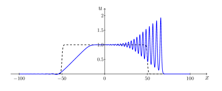
Figure 3: Evolution of a pulse with initial distribution (75) (dashed curve) over the time $t=5$ in accordance with KdV equation (9).

It is useful to briefly discuss here how a similar problem is solved in the theory of viscous shock waves (see, e.g., LL6 ). As is known, in media with weak dissipation, the wave breaking shown in Fig. 1 is eliminated due to the formation of a very thin transition domain between two states of the medium flow. Inside this domain, strong irreversible processes occur that are determined, for example, by the viscosity and heat conductance of the gas, but, farther away from this transition domain, the flow rapidly becomes an ideal gas flow, where any irreversible processes can be disregarded. In the limit of vanishing viscosity, heat conductance, and other characteristics of dissipative processes, the thickness of the transition domain in our macroscopic description tends to zero and we can replace it with a discontinuity surface of the hydrodynamic variables, with the flow considered dissipation-free on both sides of the surface. The characteristics of the flow and of the thermodynamic state of the gas must satisfy the conditions of mass, momentum, and energy conservation in the transition across the discontinuity, which determine the law of motion of the discontinuity.

In our case of interest, DSWs, we must make a similar transition to the hydrodynamic limit of vanishing dispersion. Instead of a discontinuity surface, we now have a domain of oscillations with a vanishing wavelength inside it, and the dynamics of this domain are described by Whitham modulation equations, which on ‘macroscopic’ scales also have the form of hydrodynamic first-order partial differential equations. Similarly to the case of a usual shock wave, we must incorporate a solution of these equations into the solution of the dispersionless Hopf equation, such that the smooth dispersionless solution continuously matches the averaged characteristics of the modulated oscillating solution.

It is obvious that, on the soliton edge of a DSW, this implies that the leading soliton must propagate over the background described by a smooth solution at the matching point. The situation is more delicate at the low-amplitude edge, where we should apparently expect matching with the solution of linear modulation equations (33) and (36). But in the limit of vanishing dispersion, the wave amplitude tends to zero at the matching point and Eq. (36) is satisfied in that limit automatically. Still, the conservation law for the number of waves in Eq. (43), which we used in deriving Whitham equations, turns into its linear limit (33) at the matching point. Therefore, the small-amplitude edge of the DSW moves over a smooth background with some group velocity, which in Whitham’s modulation theory becomes a hydrodynamic variable characterizing the DSW.

Indeed, taking the limit of vanishing dispersion can be formally regarded as a rescaling, i.e., a transition to ‘slow’ variables $X=\varepsilon x$ and $T=\varepsilon t$, such that the KdV equation becomes $u_{T}+6uu_{X}+\varepsilon^{2}u_{XXX}=0$, the wavelength acquires the order of magnitude $L\sim\varepsilon$, and in the limit $\varepsilon\to 0$ the last equation passes into the Hopf equation. In that same limit, the parameter $\varepsilon$ drops from the expression for the group velocity $v_{g}=-3\varepsilon^{2}k^{2}\sim(\varepsilon/L)^{2}\sim 1$, and hence the velocity of the small-amplitude DSW edge is determined only by the values of modulation parameters characterizing the DSW envelope. We emphasize that the DSW picture described here, as proposed by Gurevich and Pitaevskii, is substantially different from the earlier proposals by Benjamin-Lighthill and Sagdeev, according to which the DSW had a stationary character and its overall characteristics were determined by the mandatory existence of weak dissipation, which competed with dispersion. We return to that picture of the transition to the stationary DSW with dissipation taken into account in Section 12.

We thus assume that the breaking nonlinear solution of the dispersionless Hopf equation, Eq. (11), is modified by dispersion effects, such that, instead of a multi-valuedness domain, the domain $x_{L}<x<x_{R}$ of wave oscillations occurs in the distribution $u(x,t)$, with its evolution governed by Whitham modulation equations. Outside the domain $x_{L}<x<x_{R}$, the wave can be described by the smooth solution of the Hopf equation in Eq. (11), and inside it, the DSW is described by expression (61) with good accuracy, with the parameters $r_{1},r_{2}$, and $r_{3}$ being a solution of Whitham equations (57). This solution must satisfy boundary conditions that ensure matching with the smooth solution. To clarify the matching conditions, we note that, at these limit points, the average of $u(x,t)$ over wavelengths,

$$\langle u\rangle=2(r_{3}-r_{1})\frac{E(m)}{K(m)}+r_{1}+r_{2}-r_{3},$$ (76)

can be expressed as

$$\langle u\rangle_{r_{1}=r_{2}}=r_{3},\quad\langle u\rangle_{r_{2}=r_{3}}=r_{1}.$$ (77)

In other words, on the right edge, the value $r_{1}$ of the background over which soliton (62) is moving is equal to the value of the dispersionless solution $u(x_{R},t)$ at that point; on the left edge, the background value $r_{3}$ of small-amplitude limit (63) equals the $u(x_{L},t)$ value of the same dispersionless solution. In accordance with the foregoing assumptions, on the right edge $x_{R}(t)$, the DSW turns into a sequence of solitons, and we have $r_{2}=r_{3}$, $(m=1)$ in that case. On the left edge $x_{L}(t)$, with small amplitude of oscillations, we set $r_{2}=r_{1}$, $(m=0)$.

The coincidence of two Riemann invariants leads to the equality of the corresponding Whitham velocities (60) at the DSW edges. We obtain

$$v_{1}|_{r_{2}=r_{1}}=v_{2}|_{r_{2}=r_{1}}=12r_{1}-6r_{3},\quad v_{3}|_{r_{2}=r_{1}}=6r_{3},$$ (78)

and

$$v_{1}|_{r_{2}=r_{3}}=6r_{1},\quad v_{2}|_{r_{2}=r_{3}}=v_{3}|_{r_{2}=r_{3}}=2r_{1}+4r_{3}.$$ (79)

It then follows that, on the trailing edge $x=x_{L}(t)$, where the wave $u(x,t)$ and its averaged value coincide with the Riemann invariant $r_{3}$, its evolution is determined by the limit of Whitham equation

$$\partial r_{3}/\partial t+6r_{3}\partial r_{3}/\partial x=0,\quad r_{2}=r_{1},\quad x=x_{L}(t),$$ (80)

which coincides with Hopf equation (10) for $u(x,t)$ in the dispersionless limit. Similarly, on the leading front $x=x_{R}(t)$, where the averaged value $\langle u(x,t)\rangle$ coincides with the Riemann invariant $r_{1}$, its evolution is determined by the same Hopf equation:

$$\partial r_{1}/\partial t+6r_{1}\partial r_{1}/\partial x=0,\quad r_{2}=r_{3},\quad x=x_{R}(t).$$ (81)

We can thus conclude that the boundary condition

$$v_{1}|_{r_{1}=r_{2}}=v_{2}|_{r_{1}=r_{2}},\quad v_{3}|_{r_{1}=r_{2}}=6r_{L},$$ (82)

is satisfied at the trailing edge of the DSW, and the condition

$$v_{1}|_{r_{2}=r_{3}}=6r_{R},\quad v_{2}|_{r_{2}=r_{3}}=v_{3}|_{r_{2}=r_{3}}.$$ (83)

is satisfied at the leading edge. Here, $r_{L}$ and $r_{R}$ are the values that solution (11) of the Hopf equation, which corresponds to the initial profile $r=u_{0}(x)$, takes at the DSW matching points. For the solution of form (64), the DSW endpoints must match solution (11) of the Hopf equation, and boundary conditions (82) and (83) can be represented as

$$w_{1}|_{r_{1}=r_{2}}=w_{2}|_{r_{1}=r_{2}},\quad w_{3}|_{r_{1}=r_{2}}=\bar{x}(r_{3})$$ (84)

$$w_{1}|_{r_{2}=r_{3}}=\bar{x}(r_{1}),\quad w_{2}|_{r_{2}=r_{3}}=w_{3}|_{r_{2}=r_{3}}.$$ (85)

If we manage to find a solution of Whitham equations (57) satisfying the stated conditions, then we obtain the functions $r_{1}$, $r_{2}$, and $r_{3}$ in the entire domain $x_{L}(t)<x<x_{R}(t)$ and therefore describe the oscillating wave envelope for the entire DSW.

Before proceeding to solutions of specific problems, we note that Whitham equations, as follows from their homogeneity, have self-similar solutions of the form

$$r_{i}(x,t)=t^{\gamma}R_{i}(xt^{-1-\gamma}),$$ (86)

where $\gamma$ is an arbitrary self-similarity exponent and $R_{i}(z)$ is a solution of the system of ordinary differential equations

$$[(1+\gamma)z-v_{i}(R)]R^{\prime}_{i}=\gamma R_{i},\quad i=1,2,3,$$ (87)

where $z=xt^{-1-\gamma}$, $R^{\prime}_{i}\equiv dR_{i}/dz$, and $v_{i}(R)=t^{-\gamma}v_{i}(r)$, i.e., $v_{i}(R)$ is expressed through $R_{i}$ by the same formulas that express $v_{i}(r)$ through $r_{i}$. This remark allows finding useful classes of solutions describing DSWs for some especially chosen initial conditions.

7 Evolution of the initial discontinuity in the Korteweg-de Vries theory

We begin with the simplest example gp-73 , similar to the problem of the evolution of step-like profile (23) in the theory of the linear KdV equation. To simplify formulas, we use the fact that the KdV equation is invariant under the Galilei transformations $x\rightarrow x+6At,t\rightarrow t,u\rightarrow u+A$ and the scale transformations $x\rightarrow x/B^{1/2},t\rightarrow t/B^{3/2},u\rightarrow Bu$, where $A$ and $B$ are constant parameters. Using these transformations, the initial step-like profile of an arbitrary amplitude can be represented as

$$u_{0}(x)=u(x,0)=\begin{cases}1,&\text{ \ $x<0$},\\ 0,&\text{ \ $x>0$}.\end{cases}$$ (88)

In the dispersionless approximation, we obtain the formal solution of the Hopf equation,

$$u(x,t)=\begin{cases}1,&\text{ \ $x<6t$},\\ x/(6t),&\text{ \ $0\leq x\leq 6t$},\\ 0,&\text{ \ $x>6t$},\end{cases}$$

which is multi-valued in the domain $0<x<6t$. According to Gurevich and Pitaevskii, a DSW emerges instead of this domain when taking dispersion into account, with the DSW evolution governed by Whitham’s equations.

In Whitham’s hydrodynamic approximation, initial conditions contain no parameters of the dimension of length, and hence the solution of modulation equations must be self-similar (see (86 with $\gamma=0$), i.e., $r_{i}=r_{i}(z),z=x/t$, where $r_{i}(z)$ satisfy the differential equations $(v_{i}-z)\cdot{dr_{i}}/{dz}=0$ (see (87)). On the trailing edge $z=z_{L}$, where the oscillation amplitude tends to zero, we have $r_{1}=r_{2}$, and the averaged value $\langle{u}\rangle$ coincides with $u=1$ (see (77)), the boundary condition $r_{1}(z_{L})=r_{2}(z_{L}),r_{3}(z_{L})=1$ must hold. On the leading soliton front $z=z_{R}$, where $r_{2}=r_{3}$ and the averaged value $\langle{u}\rangle=r_{1}$ vanishes, we have another boundary condition: $r_{2}(z_{R})=r_{3}(z_{R}),r_{1}(z_{R})=0$. It is easy to see that we obtain a solution satisfying both boundary conditions if we set

$$r_{1}\equiv 0,\quad r_{3}\equiv 1,\quad v_{2}=z.$$ (89)

Then, $m=(r_{2}-r_{1})/(r_{3}-r_{1})=r_{2}$ and the last equation in (89) determines the dependence of the self-similar variable $z=x/t$ on $r_{2}$,

$$z=\frac{x}{t}=2(1+r_{2})-\frac{4r_{2}(1-r_{2})K(r_{2})}{E(r_{2})-(1-r_{2})K(r_{2})}.$$ (90)

Taking the limit $r_{2}\rightarrow 0$, we find the value of the self-similar variable on the trailing edge:

$$z_{L}=-6\quad\text{или}\quad x_{L}=-6t,$$ (91)

which means that the oscillation domain expands into the unperturbed domain of the pulse with the speed $s_{L}=v_{g}=-6$ equal to the group velocity of linear waves on the constant background $u=1$ with the dispersion law $\omega=6k-k^{3}$. Indeed, the group velocity $d\omega/dk=6-3k^{2}$ is $v_{g}=-6$ for the wavelength equal to $L(0)=\pi$ in accordance with (59), and hence for $k=2\pi/L=2$.

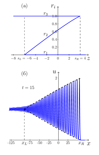
Figure 4: (a) Riemann invariants in the problem of a step-like profile. The dependence of $r_{2}$ on $z$ is defined by Eq. (90). (b)Evolution of a pulse with a step-like initial distribution in Eq. (88) driven by the KdV equation (solid line). Envelopes of the DSW amplitude are shown with dashed lines.

On the leading front, we haver $r_{2}\rightarrow 1$ and Eq. (90) implies that

$$z_{R}=4\quad\text{или}\quad x_{R}=4t,$$ (92)

and hence this DSW edge moves with the soliton speed $s_{R}=V_{s}=4r_{3}=4$. The amplitude of the leading soliton is twice the amplitude of the step-like profile. The dependence of $r_{2}=m$ on the variable $z^{\prime\prime}=4-z$, $|z^{\prime\prime}|\ll 1$ near the leading front is determined by the equation $z^{\prime\prime}\cong 2(1-m)\ln(16/(1-m))$, which gives $1-m\cong z^{\prime\prime}/2\ln(1/z^{\prime\prime})$ with logarithmic accuracy. Therefore, the distance between solitons near the leading front (where $4t-x\sim 1$ or $4-z=z^{\prime\prime}\sim 1/t$) increases with time as

$$L=2K(m)/\sqrt{r_{3}-r_{1}}\cong\pi\ln(1/z^{\prime\prime})=\pi\ln t.$$ (93)

Overall, the dependence of $r_{2}=m$ on $z$ is shown in Fig. 4(a). Substituting the values of Riemann invariants into formula (61) gives an expression for $u(x,t)$ in a DSW:

$$u(x,t)=1+r_{2}-2r_{2}\,\mathrm{sn}^{2}(x(r_{2})-2(1+r_{2})t,r_{2}),$$ (94)

with the dependence $x(r_{2})$ at a fixed instant $t$ determined by Eq. (90). Therefore, the envelope of the maxima is given by the function $u_{max}=1+r_{2}$, and the envelope of the minima, by the function $u_{min}=1-r_{2}$. In Fig. 4(b), they are shown with dashed lines. As we can see, Whitham’s theory is quite good at describing the DSW at a moderate value $t=15$, and it can be verified that the accuracy increases as $t$ increases. Whitham’s theory correctly predicts the wave number value corresponding to the small-amplitude edge of a DSW.

8 Breaking of the wave with a parabolic profile

In Section 7, we considered the simplest Gurevich-Pitaevskii problem of the formation of a DSW from a very particular initial profile, a jump-like discontinuity. Although some interesting problems can be reduced to this idealized case, including the problem of DSW generation in a flow past an obstacle gs-86 ; smyth-87 , it is rather remote from the typical wave breaking patterns. As is known (see, e.g., §101 in LL6 ), there are two main breaking scenarios for a simple wave. In the first scenario, the wave propagates into a quiescent medium and at the instant of breaking the distribution of the wave perturbation acquires a vertical tangent on the interface with the quiescent medium. In the most typical case, the wave amplitude then vanishes in accordance with a square-root law. In the second, more common, scenario, the breaking occurs as a result of the evolution of the distribution with an inflection point: at the instant of breaking, in the dispersionless approximation, this profile also acquires a vertical tangent at the inflection point, and in typical situations can be represented by a cubic parabola. In this section, we consider the first wave breaking scenario, and in Section 9 turn to the second.

We thus assume that at the instant of breaking $t=0$, the pulse amplitude vanishes in accordance with a square-root law,

$$u_{0}(x)=u(x,0)=\begin{cases}\sqrt{-x},&\text{ \ $x<0$},\\ 0,&\text{ \ $x>0$}.\end{cases}$$ (95)

Using Galilei and scaling transformations, we can bring $x|_{t=0}\propto-u^{2}$ to this simple dimensionless form. The solution of the Hopf equation with initial condition (95) is (see (11))

$$x-6ut=-u^{2},$$ (96)

showing that this solution has a domain of multi-valuedness for $0<x<9t^{2}$ after the instant of breaking $t>0$. According to the Gurevich-Pitaevskii theory, when dispersion effects are taken into account, this multi-valuedness domain is superseded by a DSW that occupies the domain $x_{L}\leq x\leq x_{R}$. On its small-amplitude trailing edge $x_{L}$, the DSW matches solution (96) (see (84)

$$w_{3}|_{r_{1}=r_{2}}=-u^{2},\quad u=r^{L}_{3}.$$ (97)

It hence follows that we must seek solution (64) with the functions $w_{i}$ that are quadratic in the Riemann invariants in the limit $m\rightarrow 0$. Velocities of this type with power-law dependences on the Riemann invariants as $m\rightarrow 0$ occur in studying generating function (74), and the required quadratic dependence corresponds to the coefficient $W^{(2)}(r_{1},r_{2},r_{3})$ at $r^{-2}$. Thus, we take $w_{i}(r)$ in form (68) with $W=W^{(2)}$, which, in view of the linearity of the Euler-Poisson equations, can be multiplied by an arbitrary constant factor $C$:

$$\begin{split}&w_{i}=C\left(1-({L}/{\partial_{i}L})\partial_{i}\right)W^{(2)}(r_{1},r_{2},r_{3}),\\ &W^{(2)}(r_{1},r_{2},r_{3})=2\sigma_{2}-\tfrac{3}{2}\sigma_{1}^{2},\\ &\sigma_{2}=r_{1}r_{2}+r_{2}r_{3}+r_{3}r_{1},\quad\sigma_{1}=r_{1}+r_{2}+r_{3}.\end{split}$$ (98)

A specific value of $C$ is determined by the condition of matching with a smooth solution on the small-amplitude DSW edge, where $r_{3}=u_{L}$. On the leading soliton edge $x_{R}$, the averaged amplitude then vanishes, and this condition yields $r_{1}=0$ and $r_{2}=r_{3}$. Hence, we can satisfy the boundary conditions by taking $r_{1}\equiv 0$ and choosing the constant $C$ such that condition (97) holds. Calculating $w_{3}$ at $m\to 0$, we obtain $w_{3}=-\frac{15}{2}Cr_{3}^{2}$, and it therefore follows from the matching condition that $C=2/15$. Finally, we obtain formulas for a solution of Whitham’s equations gkm-89 ; ks-90

$$\begin{split}&x-v_{2}t=\tfrac{2}{15}\left[W+\left(\tfrac{1}{2}v_{2}-\sigma_{1}\right){\partial W}/{\partial r_{2}}\right],\\ &x-v_{3}t=\tfrac{2}{15}\left[W+\left(\tfrac{1}{2}v_{3}-\sigma_{1}\right){\partial W}/{\partial r_{3}}\right],\end{split}$$ (99)

where $W=2r_{2}r_{3}-\frac{3}{2}(r_{2}+r_{3})^{2}$, $\sigma_{1}=r_{2}+r_{3}$.

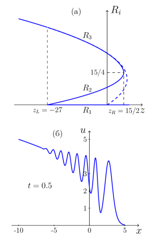
Figure 5: (a)Riemann invariants in the problem of breaking of a parabolic-profile pulse. The dashed line shows the corresponding solution $z-6R=-R^{2}$ of the Hopf equation. (b) Evolution of the pulse with initial profile (95) in accordance with the Gurevich-Pitaevskii theory for the KdV equation.

On the small-amplitude edge, these equations reduce to $x_{L}+6r_{3}^{L}t=\tfrac{1}{3}(r_{3}^{L})^{2},x_{L}-6r_{3}^{L}t=-(r_{3}^{L})^{2},$ which immediately implies the parametric representation $x_{L}=-\tfrac{1}{3}(r^{L})^{2},t=\tfrac{1}{9}r^{L},$ of the law of motion of this edge, and hence eliminating $r^{L}$ leads to

$$x_{L}=-27t^{2}.$$ (100)

On the soliton edge at $r_{2}=r_{3}$, both equations (99) tend to the same limit $x_{R}-4r_{3}t=-\tfrac{8}{15}r_{3}^{2}$, and the value of $r^{R}_{3}$ is determined by the maximum value of $x$ in the DSW domain, whence $r_{3}^{R}=15t/4$ and

$$x_{R}=\frac{15}{2}t^{2}.$$ (101)

This is the law of motion of the leading soliton edge.

It follows from the obtained formulas that we have arrived at a self-similar solution of Whitham’s equations (see (86)) with $\gamma=1$, where the Riemann invariants are

$$r_{1}=R_{1}\equiv 0,\quad r_{2}=tR_{2}(z),\quad r_{3}=tR_{3}(z)$$ (102)

with the self-similarity variable $z=x/t^{2}$. The dependence of the Riemann invariants $R_{i}$ on $z$ is shown in Fig. 5(a). It is clear that $R_{3}$ matches the solution of the Hopf equation shown in the figure with a dashed line. Substituting the found values of $r_{2}$ and $r_{3}$, together with $r_{1}=0$, into Eq. (61), we obtain a parametric form of $u(x,t)$ as a function of the coordinate and time in the DSW domain. An example of such a dependence $u(x,t)$ at a fixed instant $t$ is shown in Fig. 5(b).

9 Breaking of a cubic profile

As we have noted, typical wave breaking occurs when the initial wave profile has an inflection point and in the dispersionless limit of the solution of the Hopf equation acquires a vertical tangent at some instant. Because this breaking point remains an inflection point, the second derivative of the profile also vanishes at that point. Assuming that the third derivative of the profile does not vanish at that point, and also choosing the origin at the breaking point and the instant of breaking as zero time, we can approximate the profile near the inflection point with a cubic parabola. As a result, we obtain a solution of the dispersionless Hopf equation corresponding to the initial condition $\bar{x}(u)=-u^{3}$ at $t=0$ in the form

$$x-6ut=-u^{3}.$$ (103)

It is obvious from the foregoing that this is the most typical distribution at the instant of breaking, and we here discuss the evolution of the corresponding DSW. The main features of the solution were investigated in gp-73 , and an exact analytic solution was obtained in potemin-88 .

To solve the problem, we note that the velocities $w_{i}(r)$ in (68) that correspond to the third term $W=W^{(3)}$ in the expansion of generating function (74) have a cubic dependence on $r_{i}$ at the endpoints with $m=0$ and $m=1$. Using the formula (see (67))

$$w_{i}=\left(1-({L}/{\partial_{i}L})\partial_{i}\right)W^{(3)}(r_{1},r_{2},r_{3}),$$ (104)

where

$$W^{(3)}(r_{1},r_{2},r_{3})=-\frac{5}{4}\sigma_{1}^{3}+3\sigma_{1}\sigma_{2}-2\sigma_{3},$$ (105)

and $\sigma_{i}$ are coefficients of polynomial (70), it is easy to evaluate

$$\begin{split}&w_{3}=-\frac{35}{4}r_{3}^{3}\quad\text{при}\quad m\rightarrow 0,\\ &w_{1}=-\frac{35}{4}r_{1}^{3}\quad\text{при}\quad m\rightarrow 1.\end{split}$$ (106)

Multiplying $w_{i}$ by $-4/35$, we satisfy the boundary conditions of DSW matching on the edges with a smooth dispersionless solution in Eq. (103), and we find a solution of Whitham’s equations (57) in the form

$$x-6v_{i}(r_{1},r_{2},r_{3})t=\frac{4}{35}w_{i}(r_{1},r_{2},r_{3}),\quad i=1,2,3,$$ (107)

where the functions $w_{i}$, $i=1,2,3$, are defined by Eqs. (104 and 105). The expressions for $v_{i}$ and $w_{i}$ , even if somewhat bulky, can be given in terms of elliptic integrals as functions of the Riemann invariants (explicit formulas are presented below in a self-similar form; see Eqs. (134)-(136)). Therefore, system (107) allows finding $r_{i}$ as functions of $x$ and $t$. Before passing to the self-similar form, we consider characteristic properties of the obtained solution.

On the small-amplitude edge, we have $r_{1}=r_{2}$ ($m=0$), and Eq. (107) with $i=3$ becomes

$$x-6r_{3}t=-r_{3}^{3}\quad\text{(at $r_{1}=r_{2}$)}.$$ (108)

Similarly, on the soliton edge, we have $r_{2}=r_{3}$, and Eq. (107) with $i=1$ becomes

$$x-6r_{1}t=-r_{1}^{3}\quad\text{(at $r_{2}=r_{3}$)}.$$ (109)

Therefore, these Riemann invariants match the smooth solution on the DSW edges, as they should:

$$\begin{split}&r_{3}=u\quad\text{at}\quad r_{1}=r_{2},\\ &r_{1}=u\quad\text{at}\quad r_{2}=r_{3},\end{split}$$ (110)

where $u$ is the solution (103) of the Hopf equation. In the neighborhood of the trailing small-amplitude edge, we introduce a local coordinate $x^{\prime}$,

$$x=x_{L}+x^{\prime},$$ (111)

and small deviations $r^{\prime}_{i}$ of the Riemann invariants from their limit values,

$$r_{1}=r_{1}^{L}+r_{1}^{\prime},\quad r_{2}=r_{1}^{L}+r_{2}^{\prime},\quad r_{3}=r_{3}^{L}+r_{3}^{\prime}.$$ (112)

Expanding Eqs. (107) in powers of $r^{\prime}_{i}$ at a fixed instant $t$, we obtain

$$\begin{split}x^{L}&+x^{\prime}-(12r_{1}-6r_{3})t-(9r_{1}^{\prime}+3r_{2}^{\prime}-6r_{3}^{\prime})t\\ &=\tfrac{1}{5}(-16r_{1}^{3}+8r_{1}^{2}r_{3}+2r_{1}r_{3}^{2}+r_{3}^{3})-\\ &-\tfrac{3}{10}(24r_{1}^{2}-8r_{1}r_{3}-r_{3}^{2})r_{1}^{\prime}\\ &-\tfrac{1}{10}(24r_{1}^{2}-8r_{1}r_{3}-r_{3}^{2})r_{2}^{\prime}+\\ &+\tfrac{1}{5}(8r_{1}^{2}+4r_{1}r_{3}+3r_{3}^{2})r_{3}^{\prime},\\ x^{L}&+x^{\prime}-(12r_{1}-6r_{3})t-(3r_{1}^{\prime}+9r_{2}^{\prime}-6r_{3}^{\prime})t=\\ &=\tfrac{1}{5}(-16r_{1}^{3}+8r_{1}^{2}r_{3}+2r_{1}r_{3}^{2}+r_{3}^{3})-\\ &-\tfrac{1}{10}(24r_{1}^{2}-8r_{1}r_{3}-r_{3}^{2})r_{1}^{\prime}-\\ &-\tfrac{3}{10}(24r_{1}^{2}-8r_{1}r_{3}-r_{3}^{2})r_{2}^{\prime}+\\ &+\tfrac{1}{5}(8r_{1}^{2}+4r_{1}r_{3}+3r_{3}^{2})r_{3}^{\prime},\\ x^{L}&+x^{\prime}-6r_{3}t-6r^{\prime}_{3}t=-r^{3}_{3}-3r_{3}^{2}r_{3}^{\prime},\end{split}$$ (113)

where we introduce the temporary notation $r_{1}\equiv r_{1}^{L}$ and $r_{3}\equiv r_{3}^{L}$. Subtracting the second equation from the first, we obtain the relation

$$t=\frac{1}{30}(24r_{1}^{2}-8r_{1}r_{3}-r_{3}^{2}).$$ (114)

It hence follows that the coefficients in front of $r^{\prime}_{1}$ and $r^{\prime}_{2}$ in the first two equations in (113) vanish, and therefore $x^{\prime}$ is a quadratic function of $r^{\prime}_{1}$ and $r^{\prime}_{2}$:

$$x^{\prime}\propto{r_{1}^{\prime}}^{2},{r_{2}^{\prime}}^{2},r_{3}^{\prime}.$$

At the point $x^{L}$, these two equations give

$$x^{L}-(12r_{1}-6r_{3})t=\frac{1}{5}(-16r_{1}^{3}+8r_{1}^{2}r_{3}+2r_{1}r_{3}^{2}+r_{3}^{3}),$$ (115)

and the third equation in (113), as we have already noted, reduces to the solution $x^{L}-6r_{3}t=-r_{3}^{3}$ of the Hopf equation. We can hence find the law of motion of the trailing edge. Subtracting Eq. (108) with $x=x^{L}$ from (115) and dividing the result by $(r_{1}-r_{3})$, we obtain the relation

$$t=\frac{1}{30}(8r_{1}^{2}+4r_{1}r_{3}+3r_{3}^{2}),$$

Comparing this with (114), we find the relation between values of Riemann invariants on the trailing edge:

$$r_{1}^{L}=r_{2}^{L}=-\frac{1}{4}r_{3}^{L}.$$ (116)

It then follows from Eqs. (114) and (108) that

$$t=\frac{1}{12}(r_{3}^{L})^{2},\quad x^{L}=-\frac{1}{2}(r_{3}^{L})^{3},$$ (117)

and hence the small-amplitude edge moves according to the law

$$x^{L}=-12\sqrt{3}\,t^{3/2}.$$ (118)

The amplitude of oscillations here tends to zero as

$$a=r_{2}-r_{1}\simeq 2r_{2}^{\prime}\propto\sqrt{x^{\prime}},$$ (119)

Near the leading soliton front, we introduce small variables:

$$x=x^{R}-x^{\prime\prime},\quad x^{\prime\prime}>0,$$ (120)

$$r_{1}=r_{1}^{R}+r_{1}^{\prime\prime},\quad r_{2}=r_{3}^{R}+r_{2}^{\prime\prime},\quad r_{3}=r_{3}^{R}+r_{3}^{\prime\prime}.$$ (121)

The expansions of Eqs. (73) with only the leading corrections retained have the form

$$\begin{split}&x^{R}-x^{\prime\prime}-6r_{1}t+\left[\frac{8(r_{3}-r_{1})}{\ln(16/(1-m))}\right]t=\\ &=-r_{1}^{3}+\frac{4}{35}(15r_{1}^{2}+12r_{1}r_{3}+8r_{3}^{2})\left[\frac{r_{3}-r_{1}}{\ln(16/(1-m))}\right],\\ &x^{R}-x^{\prime\prime}-(2r_{1}+4r_{3})t+2\ln(16/(1-m))(r_{3}^{\prime\prime}-r_{2}^{\prime\prime})t=\\ &=-\tfrac{1}{35}(5r_{1}^{3}+6r_{1}^{2}r_{3}+8r_{1}r_{3}^{2}+16r_{3}^{2})\\ &+\tfrac{1}{35}(3r_{1}^{2}+8r_{1}r_{3}+24r_{3}^{2})\ln(16/(1-m))(r_{3}^{\prime\prime}-r_{2}^{\prime\prime}),\\ &x^{R}-x^{\prime\prime}-(2r_{1}+4r_{3})t-2\ln(16/(1-m))(r_{3}^{\prime\prime}-r_{2}^{\prime\prime})t=\\ &=-\tfrac{1}{35}(5r_{1}^{3}+6r_{1}^{2}r_{3}+8r_{1}r_{3}^{2}+16r_{3}^{2})\\ &-\tfrac{1}{35}(3r_{1}^{2}+8r_{1}r_{3}+24r_{3}^{2})\ln(16/(1-m))(r_{3}^{\prime\prime}-r_{2}^{\prime\prime}),\end{split}$$ (122)

where $1-m=(r_{3}^{\prime\prime}-r_{2}^{\prime\prime})/(r_{3}-r_{1})$, and we revert to the temporary notation $r_{1}\equiv r_{1}^{R}$ and $r_{3}\equiv r_{3}^{R}$. Subtracting the third equation in (122) from the second, we obtain the relation

$$t=\frac{1}{70}(3r_{1}^{2}+8r_{1}r_{3}+24r_{3}^{2}),$$ (123)

which together with the leading approximation in Eqs.(122),

$$\begin{split}x^{R}&-6r_{1}t=-r_{1}^{3},\\ x^{R}&-(2r_{1}+4r_{3})t=\\ &=-\frac{1}{35}(5r_{1}^{3}+6r_{1}^{2}r_{3}+8r_{1}r_{3}^{2}+16r_{3}^{3}),\end{split}$$ (124)

defines the law of motion of the leading edge. Indeed, the difference between Eqs. (124) gives another relation,

$$t=\frac{1}{70}(15r_{1}^{2}+12r_{1}r_{3}+8r_{3}^{2}),$$ (125)

which, when compared with (123), yields

$$r_{3}^{R}=-\frac{3}{4}r_{1}^{R},\quad(r_{1}^{R}<0),$$ (126)

whence

$$t=\frac{3}{20}(r_{1}^{R})^{2},\quad x^{R}=\frac{1}{10}|r_{1}^{+}|^{3}$$ (127)

and therefore the soliton edge moves in accordance with the law

$$x^{R}=\frac{4}{9}\sqrt{15}\,t^{3/2}.$$ (128)

The distance between solitons on the leading edge depends on $x^{\prime\prime}$ x 00 as

$$L\propto\ln(1/|x^{\prime\prime}|).$$ (129)

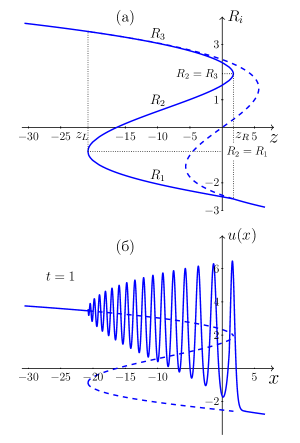
Figure 6: (a) Riemann invariants in the problem of breaking of a cubic-profile pulse. The dependence of $R_{i}=r_{i}/t^{1/2}$ on $z=x/t^{3/2}$ is determined by Eqs. (134). The dashed line shows the corresponding solution $z-6R=-R^{3}$ of the Hopf equation. (b) Evolution of the pulse with the initial cubic profile in accordance with Whitham’s approximation for the KdV equation. The dashed line shows the dependence of Riemann invariants on the coordinate $x$. The evolution time is $t=1$.

The obtained solution, which can be written in the self-similar form

$$r_{i}=t^{1/2}R_{i}\left(x/t^{3/2}\right),$$ (130)

is a solution of Eqs. (87) with $\gamma=1/2$:

$$\frac{dR_{i}}{dz}=\frac{R_{i}}{3z-v_{i}(R)}\quad z=x/t^{3/2}.$$ (131)

The above relations allow easily finding boundary values of $R_{i}$. On the trailing small-amplitude edge of the DSW, we have $z^{L}=x^{L}/t^{3/2}=-12\sqrt{3}$ and

$$R_{1}^{L}=R_{2}^{L}=-\frac{1}{2}\sqrt{3},\quad R_{3}^{L}=2\sqrt{3},$$ (132)

and on the leading soliton edge, $z^{R}=4\sqrt{15}/9$ and

$$R_{1}^{R}=-\frac{2}{3}\sqrt{15},\quad R_{2}^{R}=-R_{3}^{R}=-\frac{1}{2}\sqrt{15}.$$ (133)

The global dependence of $R_{i}$ on z $z$ defined implicitly by the expressions

$$z=6v_{1}-w_{1},\quad z=6v_{2}-w_{2},\quad z=6v_{3}-w_{3},$$ (134)

where

$$\begin{split}v_{1}=&2(R_{1}+R_{2}+R_{3})+\frac{4(R_{2}-R_{1})K(m)}{E(m)-K(m)},\\ v_{2}=&2(R_{1}+R_{2}+R_{3})-\\ -&\frac{4(R_{2}-R_{1})(1-m)K(m)}{E(m)-(1-m)K(m)},\\ v_{3}=&2(R_{1}+R_{2}+R_{3})+\\ &+\frac{4(R_{3}-R_{1})(1-m)K(m)}{E(m)};\end{split}$$ (135)

with $m=(R_{2}-R_{1})/(R_{3}-R_{1})$; the functions $w_{i}(R_{1},R_{2},R_{3})$ have the form

$$w_{i}=W+\left(\frac{1}{2}v_{i}-R_{1}-R_{2}-R_{3}\right)\frac{\partial W}{\partial R_{i}},$$ (136)

where

$$\begin{split}W=&\frac{4}{35}\Big{[}-\frac{5}{4}(R_{1}+R_{2}+R_{3})^{3}+3(R_{1}+R_{2}+R_{3})\times\\ &\times(R_{1}R_{2}+R_{2}R_{3}+R_{3}R_{1})-2R_{1}R_{2}R_{3}\Big{]}.\end{split}$$

Thus, system of algebraic equations (134) allows finding the dependence of the invariants $R_{i}$ on $z$ potemin-88 . This dependence is shown in Fig. 6(a), where the dashed line shows the cubic curve $z=6R-R^{3}$ matching the Riemann invariants $R_{3}$ and $R_{1}$ at the respective points $z^{L}$ and $z^{R}$. With the dependence of the invariants $r_{i}=t^{1/2}R_{i}(x/t^{3/2})$ on the self-similar variable found, their substitution in (61) gives a description of the DSW forming in the neighborhood of the breaking point due to dispersion effects. This DSW is plotted in Fig. 6(b). The self-similar solution considered here is valid for as long as the smooth part of the solution is described by cubic curve (103) with sufficient accuracy.

10 Motion of edges of dispersive shock waves

The solutions found in Sections 8 and 9 give an idea of the nature of the DSW evolution at a stage not too distant in time from the wave breaking instant, when the smooth part of the solution remains a monotonic function of the coordinate and is sufficiently close to a parabola or a cubic parabola. But in practice the pulses typically have a finite duration, which raises a question about the DSW shape at the stage when its full length is comparable to or much greater than the initial length of the pulse. The hodograph method outlined in Section 5 allows obtaining a solution to such a problem in the form of a solution to the system of Euler-Poisson equations (73) gkm-89 ; gke-91 ; gkme-92 ; gke-92 ; ek-93 ; kud-92 ; wright-93 ; tian-93 . However, this form of the solution is rather complicated, and even a very detailed quantitative description of the process does not give an intuitively clear picture of the effect. We therefore do not go into the details of that theory and discuss a simpler approach gkm-89 ; kamch-19 , which readily yields simple formulas for the principal parameters of the DSW and, in addition, allows a generalization to a rather broad class of other nonlinear wave equations.

We first note that ‘positive’ and ‘negative’ pulses with the respective initial distributions $u_{0}(x)>0$ and $u_{0}(x)<0$ must be distinguished: they exhibit qualitatively different behaviors and must be considered separately. An idea of how they evolve can be gleaned from Fig. 7, where we show the results of a numerical solution of the KdV equation with appropriate initial data.

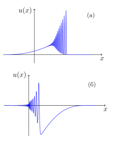
Figure 7: (a) Evolution of a ‘positive’ initial pulse. (b) Evolution of a ‘negative’ initial pulse.

For a positive pulse, breaking occurs on the leading front, and the leading part of the DSW consists of a sequence of solitons (62), moving over the zero background, whereas the trailing small-amplitude edge matches the smooth solution and propagates over an inhomogeneous background. It must be recalled here that, in the case of a localized initial pulse $u_{0}(x)$ with a single maximum $u_{m}$ of the distribution at $x=x_{m}$ (Fig. 8(a)), the inverse function consists of two branches, ${\overline{x}}_{1}(u)$ and ${\overline{x}}_{2}(u)$ (Fig. 8(b)), and hence the dispersionless solution is given by two formulas (11), one for each branch.

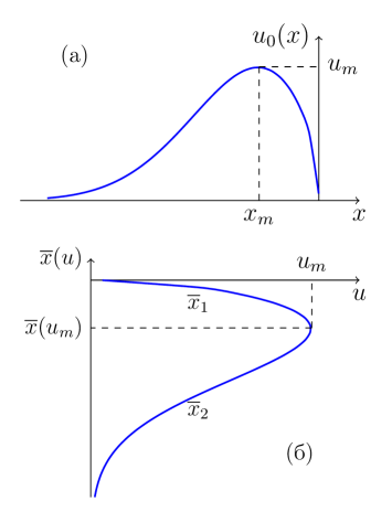
Figure 8: (a) Initial profile of a ‘positive’ pulse. (b) The inverse function ${\overline{x}}(u)$ consisting of two branches, ${\overline{x}}_{1}(u)$ and ${\overline{x}}_{2}(u)$.

At the initial stage of the DSW evolution, its small-amplitude edge matches the solution corresponding to the branch ${\overline{x}}_{1}(u)$, and at the matching point $x_{L}$ we have

$$x_{L}-6ut={\overline{x}}_{1}(u).$$ (137)

On the other hand, at that point the Riemann invariants $r_{1},r_{2}$ are equal to zero and $r_{3}=u$ (Fig. 9(a)), wavelength (59) becomes $L=\pi/\sqrt{u}$, with the corresponding wave number $k=2\sqrt{u}$, and the velocity of motion of this point, determined by the group velocity of the linear wave on the background $u$, is equal to $v_{g}=6u-3k^{2}=-6u$. Hence, $dx_{L}+6udt=0$ along the path of the small-amplitude edge, and the compatibility condition between Eq. (137) and the equation

$$\frac{dx_{L}}{du}+6u\frac{dt}{du}=0$$ (138)

leads to the differential equation

$$2u\frac{dt}{du}+t=-\frac{1}{6}\frac{d{\overline{x}}_{1}}{du},$$ (139)

which can be easily solved with the initial condition $t(0)=0$, assuming that the breaking occurs at the zero instant on the interface with the medium ‘at rest’, where $u=0$. We hence obtain

$$t(u)=\frac{1}{12\sqrt{u}}\int_{{\overline{x}}_{1}(u)}^{0}\frac{dx}{\sqrt{u_{0}(x)}},$$ (140)

and substituting this into (137) gives the law of motion of the small-amplitude edge in parametric form:

$$x_{L}(u)={\overline{x}}_{1}(u)+\frac{\sqrt{u}}{2}\int_{{\overline{x}}_{1}(u)}^{0}\frac{dx}{\sqrt{u_{0}(x)}}.$$ (141)

It is easy to verify that these formulas reproduce law (100) for the parabolic initial profile $u_{0}(x)=\sqrt{-x}$ with a single branch of the inverse function ${\overline{x}}_{1}(u)=-u^{2}$.

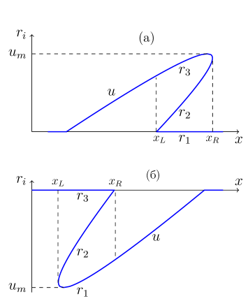
Figure 9: (a) Diagram of Riemann invariants for a ‘positive’ pulse. (b) Diagram of Riemann invariants for a ‘negative’ pulse.

For a localized initial pulse, the obtained solution is valid until the instant

$$t_{m}=\frac{1}{12\sqrt{u_{m}}}\int_{x_{m}}^{0}\frac{dx}{\sqrt{u_{0}(x)}},$$ (142)

when the small-amplitude edge reaches the point corresponding to the maximum amplitude $u_{m}$. After that, we must solve Eq. (139) with the replacement ${\overline{x}}_{1}(u)\rightarrow{\overline{x}}_{2}(u)$ and with the initial condition $t(u_{m})=t_{m}$. As a result, we obtain the law of motion of the small-amplitude edge in parametric form:

$$\begin{split}&t(u)=\frac{1}{12\sqrt{u}}\int_{{\overline{x}}_{2}(u)}^{0}\frac{dx}{\sqrt{u_{0}(x)}},\\ &x_{L}(u)={\overline{x}}_{2}(u)+\frac{\sqrt{u}}{2}\int_{{\overline{x}}_{2}(u)}^{0}\frac{dx}{\sqrt{u_{0}(x)}},\end{split}$$ (143)

where $u_{0}(x)$ is understood as the full initial profile of the pulse, vanishing at $x=0$ and tending to zero as $x\to-\infty$. If the initial pulse vanishes on the trailing edge at $x=-l\equiv{\overline{x}}_{2}(0)$, then, as $t\to\infty$, it is obvious that $t\approx\mathcal{A}/(12\sqrt{u})$, where $\mathcal{A}=\int_{-l}^{0}dx/\sqrt{u_{0}(x)}$, and the law of motion of the trailing edge takes the asymptotic form

$$x_{L}\approx-l+\frac{\mathcal{A}^{2}}{24t},\quad t\to\infty.$$ (144)

The asymptotic form of the law of motion can also be easily found for the leading soliton edge of the DSW. We see from Fig. 9(a) for Riemann invariants that, as $t\to\infty$, the plots of $r_{2}(x)$ and $r_{3}(x)$ elongate into an extended ‘tongue’, with $r_{1}=0$ and $r_{2}\approx r_{3}\approx u_{m}$ near the leading edge. Therefore, the leading edge moves with the soliton velocity $V_{s}\approx 4u_{m}$ and

$$x_{R}\approx 4u_{m}t.$$ (145)

Turning now to the question of the evolution of a negative initial pulse, we see from Fig. 7(b) that the smooth dispersionless solution is adjacent to the soliton edge of the DSW, which therefore propagates over an inhomogeneous background. On that boundary, the Riemann invariants are $r_{1}=u$ and $r_{2}=r_{3}=0$ and (Fig. 9(b)), and hence the soliton edge velocity is $V_{s}=2u$ or $dx_{R}=2udt$, in accordance with (79)

$$\frac{dx_{R}}{du}-2u\frac{dt}{du}=0$$ (146)

must again be made compatible with the dispersionless solution

$$x_{R}-6ut={\overline{x}}_{i}(u),\quad i=1,2,$$ (147)

if the edge borders the $i$th branch of that solution. Eliminating $x_{R}$, we obtain a differential equation for $t=t(u)$:

$$2u\frac{dt}{du}+3t=-\frac{1}{2}{\overline{x}}_{i}^{\prime}(u),$$ (148)

where ${\overline{x}}_{i}(u)$ is the corresponding branch of the inverse function of the initial distribution (Fig. 10). For the branch $i=1$, a solution is sought with the initial condition $t(0)=0$, which defines a parametric form of the law of motion of the soliton edge:

$$\begin{split}&t(u)=\frac{1}{4(-u)^{3/2}}\int_{0}^{u}\sqrt{-u}\,{\overline{x}}_{1}^{\prime}(u)du,\\ &x_{R}=-\frac{3}{2\sqrt{-u}}\int_{0}^{u}\sqrt{-u}\,{\overline{x}}_{1}^{\prime}(u)du+{\overline{x}}_{1}(u).\end{split}$$ (149)

For example, for a parabolic initial pulse $u_{0}(x)=-\sqrt{x}$, ${\overline{x}}_{1}(u)=u^{2}$, $x>0$, we hence find the law of motion $x_{R}=-5t^{2}$.

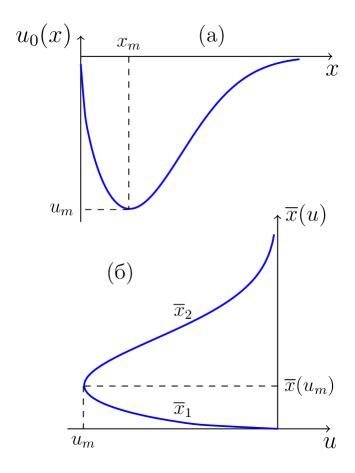
Figure 10: (a) Initial profile of a ‘negative’ pulse. (b) The inverse function ${\overline{x}}(u)$ consisting of two branches, ${\overline{x}}_{1}(u)$ and ${\overline{x}}_{2}(u)$.

Solving Eq. (148) with the initial condition

$$t(u_{m})=\frac{1}{4(-u_{m})^{3/2}}\int_{0}^{u_{m}}\sqrt{-u}\,{\overline{x}}_{1}^{\prime}(u)du$$

for a localized initial pulse with a minimum $u=u_{m}$ at $x=x_{m}$, we obtain the law of motion

$$\begin{split}&t(u)=\frac{1}{4(-u)^{3/2}}\int_{0}^{x_{2}(u)}\sqrt{-u_{0}(x)}\,dx,\\ &x_{R}=x_{2}(u)-\frac{3}{2\sqrt{-u}}\int_{0}^{x_{2}(u)}\sqrt{-u_{0}(x)}\,dx.\end{split}$$ (150)

Negative solitons are nonexistent for the KdV equation, and therefore a negative pulse cannot decay into a sequence of solitons at asymptotically large times. Instead, it transforms into a nonlinear wave packet whose soliton edge moves at $t\to\infty$ in accordance with the law

$$x_{R}\approx-\frac{3\mathcal{A}^{2/3}}{2^{1/3}}t^{1/3},\quad\mathcal{A}=\int_{0}^{\infty}\sqrt{-u_{0}(x)}\,dx,$$ (151)

matching a virtually rectilinear asymptotic dispersionless solution $u\approx x/(6t)$ for $x_{R}<x<0$. Accordingly, the leading soliton amplitude in the DSW decreases with time as

$$a=2|r_{1}|\approx\frac{\mathcal{A}^{2/3}}{2^{4/3}}t^{-2/3}.$$ (152)

Near this edge, solutions of Whitham’s equations are self-similar and depend on the variable $z=x/t^{1/3}$. Although this solution can be obtained in analytic form dvz-94 ; ikp-19 , the self-similarity domain is relatively small, and we do not discuss this theory here. The solution of Whitham’s equations in the entire DSW domain was obtained in ek-93 ; ikp-19 . In approaching the small-amplitude edge, the DSW evolution again becomes self-similar, with the modulation parameters depending on $z=x/t$. We can obtain the asymptotic law of motion of the small-amplitude edge by noting that, according to Fig. 9(b), $r_{1}\approx r_{2}\approx u_{m}$ and $r_{3}=0$ on that edge, and hence from (59) we can find the wave number $k=2\pi/L\approx 2\sqrt{-u_{m}}$. Therefore, at the matching point, the group velocity of the linear wave is $v_{g}=-3k^{2}=-12u_{m}$ and

$$x_{L}\approx-12u_{m}t.$$ (153)

11 Theorem on the number of oscillations in dispersive shock waves

An important theorem given in gp-87 states that, due to the difference between the velocity of the small-amplitude edge $v_{g}$ and the phase velocity of the wave $V$, the DSW length increases on that edge by $(v_{g}-V)dt$ in a time $dt$, and therefore the number of wave periods in the domain of oscillations increases with the rate

$$\frac{dN}{dt}=\frac{1}{2\pi}k(v_{g}-V),$$ (154)

where all the variables are evaluated at the DSW wave number on the small-amplitude edge. The right-hand side of rem1 can also be interpreted as the flux of the wave number $\omega=kV$ into the DSW domain with a Doppler shift due to the motion of the boundary, with the speed $v_{g}$ taken into account. Therefore, the total number of oscillations entering the DSW over all of its evolution time is up to a sign given by

$$N=\frac{1}{2\pi}\int_{-\infty}^{\infty}k(v_{g}-V)dt=\frac{1}{2\pi}\int_{-\infty}^{\infty}\left(k\frac{d\omega}{dk}-\omega\right)dt.$$ (155)

The integrand can be interpreted as a Lagrangian of a classical particle with the momentum $k$ and the Hamiltonian $\omega$, which is associated with the wave packet co-moving with the small-amplitude edge of the DSW. The integral is then equal to the classical action $S$ of such a particle and the number of oscillations is

$$N=\frac{S}{2\pi}.$$ (156)

It is clear that these formulas are of a general nature and their validity is not limited to the KdV equation.

For actual calculations, we must know the main characteristics of the DSW at least on its small-amplitude edge. For example, in the case of the KdV equation, it is easy to find that $|k(v_{g}-V)|=2k^{3}$; for the evolution of a unit-height step, as shown in Section §7, the wave number on the small-amplitude edge is $k=2$. We hence find the number of oscillations formed in the DSW over time $t$: $N=(8/\pi)t$. For the time $t=15$, this formula predicts $N\approx 38$, whereas counting the oscillations in Fig.  4(b), which shows the results of a numerical solution of the KdV equation, gives approximately $N\approx 39$, in good agreement with the theory. However, the agreement with this asymptotic calculation worsens at smaller times. For example, in the case of breaking of a cubic profile, the values of Riemann invariants on the small-amplitude edge, according to formula (116), are $r_{3}=u$ and $r_{1}=r_{2}=-u/4$, where $u$ is the wave amplitude at the matching point, depending on time as $u=\sqrt{12t}$ (see (116)). Substitution into (59) gives the wavelength $L=2\pi/\sqrt{5u}$ and the wave number $k=\sqrt{5u}=\sqrt{10}\cdot 3^{1/4}t^{1/4}$. Hence, for the number of oscillations formed by the instant $t$, we obtain

$$N=\frac{40\sqrt{10}\cdot 3^{3/4}}{7\pi}t^{7/4}\approx 13,1\cdot t^{7/4}.$$

For $t=1$, the number of oscillations $N\approx 13$ is somewhat different from the number of oscillations $N\approx 15\div 16$ discernible in Fig. 6(b), but can still be considered satisfactory for such a short evolution time.

As regards a positive pulse of finite duration, it eventually evolves mainly into a sequence of solitons propagating over the zero background $u=r_{1}=0$. The group velocity of the small-amplitude edge, which is a hydrodynamic variable in Whitham’s theory, then has the meaning of the velocity of the interface between the oscillations that turn into solitons as $t\to\infty$ and the linear wave packet. The number of solitons formed from a localized pulse is determined by the initial profile $u_{0}(x)$ and can be evaluated as follows.

On the low-amplitude edge, $k=2\sqrt{u}$ and $k(v_{g}-V)=-2k^{3}=-16u^{3/2}$. Integration over $t$ from $0$ to $t_{m}$ can be replaced using (139) and (140) with integration over $u$ from $0$ to $u_{m}$, and similarly integration from $t_{m}$ to $+\infty$ transforms with the help of (143) into integration over the same interval of $u$. As a result, we obtain

$$N=\frac{4}{\pi}\int_{0}^{u_{m}}\left[t_{2}-t_{1}+\frac{1}{6}({\overline{x}}_{2}^{\prime}-{\overline{x}}_{1}^{\prime})\right]du,$$ (157)

where

$$t_{2}-t_{1}=\frac{1}{12\sqrt{u}}\int_{u}^{u_{m}}\frac{{\overline{x}}_{2}^{\prime}-{\overline{x}}_{1}^{\prime}}{\sqrt{u_{1}}}\,du_{1}.$$ (158)

The double integral that occurs in substituting (158) into (157) can easily be made single-fold by integration by parts, which leads to the formula

$$N=\frac{1}{\pi}\int_{0}^{u_{m}}\sqrt{u}({\overline{x}}_{2}^{\prime}-{\overline{x}}_{1}^{\prime})du=\frac{1}{\pi}\int_{-\infty}^{0}\sqrt{u_{0}(x)}\,dx,$$ (159)

where, as usual, $u_{0}(x)$ is the initial profile of the wave. This formula was first derived in karpman-67 using profound mathematical properties of the KdV equation associated with its complete integrability ggkm-67 . In our presentation, it is a simple corollary of the Gurevich-Pitaevskii approach to the DSW theory.

12 Theory of dispersive shock waves for the Korteweg-de Vries equation with dissipation

In the Introduction, we discussed the development of the DSW concept, starting with Sagdeev’s idea that dispersion effects transform the transition layer of a viscous shock wave into a stationary oscillatory structure, and on to Gurevich and Pitaevskii’s idea of the formation of non-stationary DSWs as a result of wave breaking, with the evolution of the DSW modulation parameters governed by Whitham’s equations. It must be clear, however, that the existence of small dissipation or other perturbing terms in the KdV equation also leads to the evolution of modulation parameters, which means that Whitham’s modulation equations must then be modified accordingly. The picture proposed by Sagdeev must then be described by stationary solutions of modified Whitham’s equations that take small dissipation effects into account, in addition to dispersion. In this section, we discuss such a modified Whitham’s theory and the simplest corollaries.

We assume that the perturbed KdV equation has the form

$$u_{t}+6uu_{x}+u_{xxx}=R[u],$$ (160)

where the perturbing term is small, $R\sim\varepsilon\ll 1$, and depends on both the field $u$ and its spatial derivatives. Generally speaking, two types of perturbation must be distinguished. For one type, Whitham’s equations acquire right-hand sides with the old form of Riemann invariants, and perturbations of the other type lead to a non-diagonal form of the averaged equations

$$\frac{\partial r_{i}}{\partial t}+\sum_{j}v_{ij}\frac{\partial r_{j}}{\partial x}=0,$$

diagonalizing which, as noted in Section 4, is typically impossible. We discuss only the first case, which includes physically important problems with small dissipation. We again derive perturbed Whitham’s equations by averaging the conservation laws. We then take into account that the conservation law for the number of waves, Eq. (43), preserves its form, while conservation laws (44) acquire right-hand sides:

$$\begin{split}&u_{t}+(3u^{2}+u_{xx})_{x}=R,\\ &(\tfrac{1}{2}u^{2})_{t}+(2u^{3}+uu_{xx}-\tfrac{1}{2}u_{x}^{2})_{x}=uR.\end{split}$$ (161)

The averaged equations

$$\begin{split}&\langle u\rangle_{t}+\langle 3u^{2}+u_{xx}\rangle_{x}=\langle R\rangle,\\ &\langle\tfrac{1}{2}u^{2}\rangle_{t}+\langle 2u^{3}+uu_{xx}-\tfrac{1}{2}u_{x}^{2}\rangle_{x}=\langle uR\rangle\end{split}$$ (162)

can be transformed just as we did previously, and instead of (49) we now obtain the equations

$$\begin{split}&\frac{D\mathcal{W}_{A}}{Dt}=\mathcal{W}_{A}\frac{\partial V}{\partial x},\quad\frac{D\mathcal{W}_{B}}{Dt}=\mathcal{W}_{A}\frac{\partial B}{\partial x}-\mathcal{W}_{A}\langle R\rangle,\\ &\frac{D\mathcal{W}_{V}}{Dt}=\mathcal{W}_{A}\frac{\partial A}{\partial x}-\mathcal{W}_{A}\langle uR\rangle.\end{split}$$ (163)

which differ from the preceding equations only by additional termsdependingontheperturbation.Movingtothevariables $\nu_{1},\nu_{2},$ and $\nu_{3}$ and introducing Riemann invariants (55) for unperturbed Whitham’s equations as the modulation parameters, we find the desired Whitham’s equations accounting for the perturbation:

$$\begin{split}&\frac{\partial r_{i}}{\partial t}+v_{i}\frac{\partial r_{i}}{\partial x}=\frac{L}{\partial L/\partial r_{i}}\times\\ &\times\frac{\langle(\sigma_{1}-2r_{i}-u)R\rangle}{4\prod_{j\neq i}(r_{i}-r_{j})},\quad i=1,2,3,\end{split}$$ (164)

where $v_{i}$ are Whitham’s velocities (60) of the unperturbed equations and $\sigma_{1}=r_{1}+r_{2}+r_{3}$. In the particular case of Burgers viscosity, the perturbed Whitham equations were derived in gp-87 ; akn-87 , and for nonlocal viscosity, in gp-91 . In the general case, they are derived in form (164) in mg-95 ; kamch-04 ; kamch-16 .

To obtain an insight into the role of small dissipation, we turn to the Gurevich-Pitaevskii problem of the decay of an initial discontinuity. We recall from Section 7 that, at the initial stage of the evolution, dissipation is inessential and the DSW expands in a self-similar fashion. But when its length reaches a size $\sim\varepsilon^{-1}$, all terms in Whitham’s equations (164) become equally significant, and the transition to the stationary regime of propagation is to be expected, with the full size of the DSW determined by the balance of terms with derivatives with respect to coordinates and dissipative corrections. We therefore seek the solution of Whitham’s equations (164) with the invariants $r_{i}$ depending only on the variable $\xi=x-Vt$. It is a simple observation that this system reduces to

$$\frac{dr_{i}}{d\xi}=-\frac{\langle(\sigma_{1}-2r_{i}-u)R\rangle}{8\prod_{j\neq i}(r_{i}-r_{j})},\quad i=1,2,3,$$ (165)

if we take $V$ to be the wave velocity $V=2\sigma_{1}$. Because the profile is stationary, this system must have the integral

$$\sigma_{1}=\mathrm{const}.$$ (166)

It is easy to verify that $\sigma_{1}$ is indeed an integral, and the other two symmetric functions $\sigma_{2}=r_{1}r_{2}+r_{1}r_{3}+r_{2}r_{3}$ and $\sigma_{3}=r_{1}r_{2}r_{3}$ satisfy the equations

$$\frac{d\sigma_{2}}{d\xi}=\frac{1}{4}\langle R\rangle,\quad\frac{d\sigma_{3}}{d\xi}=\frac{1}{8}[\sigma_{1}\langle R\rangle-\langle uR\rangle].$$ (167)

We have thus reduced the problem to solving a system of two ordinary differential equations for $\sigma_{2}$ and $\sigma_{3}$, with $r_{i}$ being the functions of $\sigma_{2}$ and $\sigma_{3}$ to be found from the cubic equation

$$Q(r)=r^{3}-\sigma_{1}r^{2}+\sigma_{2}r-\sigma_{3}=0.$$ (168)

The problem can be simplified even more if $\langle R\rangle=0$, in which case we have another integral $\sigma_{2}=\mathrm{const}$, and it remains to solve a single differential equation,

$$\frac{d\sigma_{3}}{d\xi}=-\frac{1}{8}\langle uR\rangle.$$ (169)

It is now convenient to return from the symmetric functions to the variables $r_{i}$ and, for example, regard $r_{1}$ and $r_{2}$ as functions of $r_{3}$, where $r_{3}=r_{3}(\xi)$. From (165), we then find

$$\frac{dr_{1}}{dr_{3}}=\frac{r_{3}-r_{2}}{r_{2}-r_{1}},\quad\frac{dr_{1}}{dr_{3}}=-\frac{r_{3}-r_{1}}{r_{2}-r_{1}}.$$ (170)

This system has two integrals: $\sigma_{1}=\mathrm{const}$ and $\sigma_{2}=\mathrm{const}$. Therefore, $r_{1}$ and $r_{2}$ as functions of $r_{3}$ are the roots of the quadratic equation

$$r^{2}-(\sigma_{1}-r_{3})r+\sigma_{2}-(\sigma_{1}-r_{3})r_{3}=0.$$ (171)

Its roots must be ordered as $r_{1}\leq r_{2}$; the constants $\sigma_{1}$ and $\sigma_{2}$ are determined by the boundary conditions. We let $u_{L}$ denote the limit value of the wave amplitude as $x\to-\infty$ and assume that the wave propagates in a medium with $u=0$ at $x\to+\infty$. On the small-amplitude edge, where $m\to 0$, $r_{2}\to r_{1}$, we have $u_{L}=r_{3}=r_{3}^{L}$ and

$$\sigma_{1}=2r_{1}^{L}+u_{L},\quad\sigma_{2}=(r_{1}^{L})^{2}+2r_{1}^{L}u_{L}.$$ (172)

On the soliton edge, $r_{1}^{R}=0$ and $r_{2}^{R}=r_{3}^{R}$, and substituting these into the definition of $\sigma_{1}$ and $\sigma_{2}$ yields the relation

$$\sigma_{1}^{2}-4\sigma_{2}=0$$ (173)

between the integrals. Substituting formulas (172) into (173), we obtain an equation for $r_{1}^{L}$, whose solution gives $r_{1}^{L}=u_{L}/4$, and hence

$$\sigma_{1}=\frac{3}{2}u_{L},\quad\sigma_{2}=\frac{9}{16}u_{L}^{2}.$$ (174)

on the small-amplitude edge. The integrals take the same values as on the soliton edge, where $r_{1}=0$ and $\sigma_{3}=0$, and hence Eq. (168) has a double root $r_{2}^{R}=r_{3}^{R}=\frac{3}{4}u_{L}$. As a result, the amplitude $a_{s}=2r_{3}^{R}$ of the leading soliton and its velocity $V_{s}=4r_{3}^{R}$, coincident with the shock wave velocity, are

$$a_{s}=\frac{3}{2}u_{L},\qquad V=3u_{L}.$$ (175)

Thus, the speed of a stationary DSW is determined only by the magnitude of the discontinuity, in accordance with the general theory of viscous small-amplitude shock waves LL6 . Interestingly, not only the speed but also the amplitude of the leading soliton is expressed by universal formulas (175) in terms of the initial discontinuity and is independent of the form of the dissipative term. In the particular case of Burgers-type dissipation, formulas (175) were derived in johnson-70 directly from the perturbation theory without using Whitham’s theory.

Figure 11: (a) Plots of Riemann invariants for the stationary solution of Whitham’s equations corresponding to a DSW with Burgers viscosity (178) at $\varepsilon=0.1$, $u_{L}=1.0$. (b) Profile of a stationary shock wave $u(\xi)$ with Burgers viscosity at the same parameter values.

To find a global solution along all of the DSW, we note that, after substituting integrals (174) into (171) and solving this quadratic equation, we obtain $r_{1}$ and $r_{2}$ as functions of $r_{3}$. Their substitution into expression (59) for $m$ gives an equation whose solution for $r_{3}$ allows expressing this Riemann invariant in terms of $m$, and then $r_{1}$ and $r_{2}$ can also be represented as functions of $m$. As a result of these elementary calculations, we obtain

$$\begin{split}&r_{1}=\frac{u_{L}}{2}\left(1-\frac{1+m}{2\sqrt{1-m+m^{2}}}\right),\\ &r_{2}=\frac{u_{L}}{2}\left(1-\frac{1-2m}{2\sqrt{1-m+m^{2}}}\right),\\ &r_{3}=\frac{u_{L}}{2}\left(1+\frac{1-m/2}{\sqrt{1-m+m^{2}}}\right).\end{split}$$ (176)

The problem is solved when we obtain the dependence of the parameter $m$ on the coordinate $\xi$. Evaluating the derivative $dm/dr_{3}$ with the help of formulas (170) and multiplying the result by $dr_{3}/d\xi$ in (165), we obtain the desirable equation,

$$\frac{dm}{d\xi}=-\frac{1-m+m^{2}}{4(r_{2}-r_{1})(r_{3}-r_{1})(r_{3}-r_{2})}\langle uR\rangle,$$ (177)

where the right-hand side can be expressed in terms of $m$ for a perturbation $R$ of a given form.

We specify this theory by choosing the perturbation as Burgers friction gp-87 ; akn-87 :

$$R=\varepsilon u_{xx}.$$ (178)

To actually take the averages, it is convenient to pass to the variable $\upsilon=(\sigma_{1}-u)/2$ that satisfies the equation $\upsilon_{x}^{2}=4Q(\upsilon)$, whence $u_{xx}=-2\upsilon_{xx}=-4dQ/d\upsilon$. As a result, we find

$$-\langle uR\rangle=\frac{8\varepsilon}{L}\oint\sqrt{Q(\upsilon)}\,d\upsilon.$$

This elliptic integral is readily reduced to tabulated ones, and we hence obtain the equation

$$\begin{split}&\frac{dm}{d\xi}=\Phi(m)\equiv\frac{8\varepsilon}{15}\frac{1-m+m^{2}}{m(1-m)}\times\\ &\times\left[(1-m+m^{2})\frac{E(m)}{K(m)}-(1-m)\left(1-\frac{m}{2}\right)\right].\end{split}$$ (179)

The problem solution has thus been reduced to the quadrature

$$\xi=-\int_{m}^{1}\frac{dm}{\Phi(m)}.$$ (180)

This formula, together with (176), parametrically defines the dependence of the modulation parameters, i.e., the Riemann invariants $r_{i}$ of the system of Whitham’s equations, on the coordinate $\xi$, referenced to the DSW front. An example of such a dependence is shown in Fig. 11(a), and the corresponding DSW profile is shown in Fig. 11(b).

13 Gross-Pitaevskii equation

Besides the KdV equation, which has a universal character, another very important equation, also occurring in very diverse circumstances, is the Gross-Pitaevskii equation, which in particular describes the dynamics of a weakly non-ideal Bose gas at zero temperature gross ; pit-1 in the mean field approximation, when the coherent state of the macroscopic Bose gas is described by a classical wave function, similar to the Maxwell field in classical electrodynamics. This theory came to the forefront after the experimental realization of Bose-Einstein condensation of atoms, and the main ideas underlying the theory are available in reviews dps-99 ; pit-2 . Here, we restrict ourselves to writing the Gross-Pitaevskii equation for the wave function $\psi(\mathbf{r})$ in the standard notation:

$$i\hbar\frac{\partial\psi}{\partial t}=-\frac{\hbar^{2}}{2m}\Delta\psi+U(\mathbf{r})\psi+g|\psi|^{2}\psi,$$ (181)

where $m$ is the atom mass, $\Delta$ is the Laplace operator, $U(\mathbf{r})$ is the potential of an external field acting on the atoms, and the parameter $g$, expressed in terms of the atom-atom scattering length $a$,

$$g=\frac{4\pi\hbar^{2}a}{m}$$

characterizes the strength of interatomic interaction; it is repulsive for $g>0$ and attracting for $g<0$. We are interested in the first case, where the homogeneous state of the condensate is stable and waves can propagate over it.

We note that the mathematically equivalent equation occurred in describing self-focusing of light beams in non-linear media talanov-65 ; kelley-65 , where the role of time is played by the coordinate along the beam and diffraction replaces dispersion, but the papers just cited discussed only the focusing nonlinearity, for which the state with a homogeneous distribution of light intensity is unstable. Another interpretation of Eq. (181) occurs when describing the evolution of the envelope of a wave packet propagating in a medium with low dispersion and weak nonlinearity bn-67 . In that case, the first term on the right-hand side corresponds to second-order dispersive effects, which, besides the packet motion with the group velocity, takes its slow spreading into account, and the last term corresponds to the dependence of the medium response on the wave intensity. This situation occurs rather frequently in physics, from the description of deep-water waves to the theory of propagation of light pulses in non-linear optical fibers. In this context, the resultant equation is often called the nonlinear Schrödinger (NLS) equation, but we here use the physical interpretation due to Gross-Pitaevskii, which allows addressing more transparent representations and notions of gas dynamics. In particular, the condensate density is $\rho=|\psi|^{2}$, and its flow speed is expressed in terms of the gradient of the wave function phase dps-99 ; pit-2 . If we represent the wave function as

$$\psi=\sqrt{\rho}\,e^{i\phi},\qquad\mathbf{u}=\frac{\hbar}{m}\nabla\phi,$$ (182)

then, substituting this into (181), after simple transformations, leads to the system of equations (with $U(\mathbf{r})=0$)

$$\begin{split}&\rho_{t}+\nabla(\rho\mathbf{u})=0,\\ &\nabla\mathbf{u}+(\mathbf{u}\nabla)\mathbf{u}+\frac{g}{m}\nabla\rho+\frac{\hbar^{2}}{2m}\nabla\left[\frac{(\nabla\rho)^{2}}{4\rho^{2}}-\frac{\Delta\rho}{2\rho}\right]=0.\end{split}$$ (183)

The first equation is the standard continuity equation corresponding to the conservation of the number of particles in the condensate, and the second equation has the form of a modified Euler equation for the flow of gas with the equation of state $p=g\rho^{2}/(2m)$ and with the last term containing higher-order spatial derivatives. It is clear that this term corresponds to dispersive properties of the gas caused by quantum dispersion of atoms. If we consider extremely long waves and ignore this term, we arrive at an expression for the speed of sound in the condensate,

$$c_{s}=\sqrt{\frac{dp}{d\rho}}=\sqrt{\frac{g\rho}{m}}.$$ (184)

which depends on the local density $\rho$. If we turn to linear waves in a homogeneous condensate with a constant density $\rho$, then a standard calculation gives Bogoliubov’s dispersion law bogol-47

$$\omega(k)=k\sqrt{c_{s}^{2}+\left(\frac{\hbar k^{2}}{2m}\right)^{2}}.$$ (185)

where, as the wave number $k$ increases, the sound dispersion law $\omega=c_{s}k$ passes into the standard dispersion law of quantum particles $\varepsilon=\hbar\omega=(\hbar k)^{2}/(2m)$ when the de Broglie wavelength becomes less than the coherence length

$$\xi_{C}=\frac{\hbar}{\sqrt{2}mc_{s}}=\frac{\hbar}{\sqrt{2mg\rho}}.$$ (186)

We introduce parameters characterizing the state of the condensate: the length $\xi_{c}$ and the speed $c_{s}$ at the characteristic density $\rho_{0}$, which allows us to define convenient dimensionless variables $\mathbf{r}\to\mathbf{r}/(\sqrt{2}\xi_{C})$, $t\to c_{s}t/(\sqrt{2}\xi_{C})$, and $\psi\to\psi/\sqrt{\rho_{0}}$. In addition, we restrict ourselves in what follows to only one-dimensional motions of the condensate, and therefore, in the new variables, the Gross-Pitaevskii equation takes the form

$$i\psi_{t}+\frac{1}{2}\psi_{xx}-|\psi|^{2}\psi=0,$$ (187)

and its ‘hydrodynamic’ representation (183) becomes

$$\begin{split}&\rho_{t}+(\rho u)_{x}=0,\\ &u_{t}+uu_{x}+\rho_{x}+\left(\frac{\rho_{x}^{2}}{8\rho^{2}}-\frac{\rho_{xx}}{4\rho}\right)_{x}=0.\end{split}$$ (188)

Accordingly, for linear waves, thedispersion law in Eq. (185) becomes

$$\omega(k)=k\sqrt{1+\frac{k^{2}}{4}}.$$ (189)

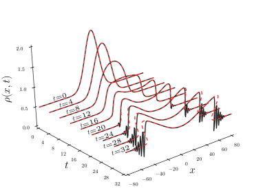
Figure 12: Evolution of an initially localized density pulse in a Bose-Einstein condensate. After the wave breaking at $t_{b}\approx 20$, DSWs emerge on the pulse edges.

It is clear that waves can propagate in both directions of the $x$ axis, and therefore any initial perturbation evolves with time into two wave pulses propagating in opposite directions. For example, if the initial pulse has a shape describing a hump in the condensate density above a homogeneous background, then the numerical solution of Gross-Pitaevskii equation (187) or the equivalent system (187) exhibits the wave evolution shown in Fig. 12. As we can see, the pulse splits into two with time, and each of them experiences breaking with the formation of a DSW. We therefore have the task to describe the evolution of shock waves satisfying the Gross-Pitaevskii equation. In accordance with the Gurevich-Pitaevskii approach, each DSW borders a smooth solution of the dispersionless equations, and we therefore first discuss this last approximation.

In the dispersionless limit, the last term in Euler equation (188) can be dropped, and the system takes the simple hydrodynamic form

$$\rho_{t}+(\rho u)_{x}=0,\quad u_{t}+uu_{x}+\rho_{x}=0.$$ (190)

As is standard in the theory of linear waves, local changes in the density $\delta\rho$ and velocity $\delta u$ of the flow are related as $\delta\rho/\rho\approx\pm\delta u/c$, where the choice of sign corresponds to the wave propagation direction. Therefore, for example, in a wave propagating to the right, the differential relation $du=cd\rho/\rho=d\rho/\sqrt{\rho}$ is satisfied, integrating which shows that, in such a simple wave, the flow velocity $u$ and the density $\rho$ are related as $u/2-\sqrt{\rho}=\mathrm{const}$, and a similar relation with the other sign in front of the square root holds for a wave propagating to the left. This argument shows that the so-called Riemann invariants, related to the density and velocity of the flow as

$$r_{+}=\frac{u}{2}+\sqrt{\rho},\quad r_{-}=\frac{u}{2}-\sqrt{\rho}.$$ (191)

are natural variables in the physics of waves. Equations (190), when written in these variables, take a simple diagonal form,

$$\begin{split}\frac{\partial r_{+}}{\partial t}+v_{+}(r_{+},r_{-})\frac{\partial r_{+}}{\partial x}=0,\\ \frac{\partial r_{-}}{\partial t}+v_{-}(r_{+},r_{-})\frac{\partial r_{-}}{\partial x}=0,\end{split}$$ (192)

where the velocities $v_{\pm}=u\pm c$ have a clear physical meaning of the signal propagation speed, equal to the sum of and the difference between the flow velocity and the speed of sound propagating downstream or upstream. In our case of the Bose-Einstein condensate, they are especially simply expressed in terms of the Riemann invariants:

$$v_{+}=\frac{3}{2}r_{+}+\frac{1}{2}r_{-},\quad v_{-}=\frac{1}{2}r_{+}+\frac{3}{2}r_{-}.$$ (193)

Simple waves are characterized by the constancy of one of the Riemann invariants. For example, for a wave propagating to the right, the invariant $r_{-}=r_{-}^{(0)}=\mathrm{const}$ is constant, the second equation in (192) is then satisfied automatically, and the first equation becomes the Hopf equation, which we already discussed in the case of ion-sound waves in plasma. Obviously, because of the relation between $\rho$ and $u$, this Hopf equation can also be written for only one of these variables, which would then give a dispersionless approximation for unidirectional propagation of waves in the condensate. Additionally taking dispersion (189) into account in the leading approximation, $\omega\approx k+k^{3}/8$, leads to the KdV equation for nonlinear waves in the limit of a large wavelength and a small amplitude. It is easy to see that the nonlinear and dispersion terms have opposite signs in this equation, and therefore soliton solutions correspond to troughs in the density distribution, and the KdV equation describes ‘shallow’ solitons on a homogeneous background. Naturally, the DSW theory for KdV is entirely applicable to the description of shock waves in a condensate under the condition of their small amplitude and unidirectional propagation. But for deep solitons and large-amplitude DSWs, development of the Gurevich-Pitaevskii theory is required.

With the dispersionless approximation equations conveniently written in form (192), we can now turn to the theory of periodic solutions of the Gross-Pitaevskii equation, whose modulations describe the DSWs. If we seek a solution to system (188) in the form of a traveling wave $\rho=\rho(\xi)$, $u=u(\xi)$, $\xi=x-Vt$, then the first equation is readily integrated, and the second, after eliminating the variable $u$ and some transformations, reduces to the equation

$$\rho_{\xi}=2\sqrt{\mathcal{R}(\rho)},\quad\mathcal{R}(\rho)=\prod_{i=1}^{3}(\rho-\nu_{i}).$$ (194)

Evidently, the density $\rho$ oscillates in the range $\nu_{1}\leq\rho\leq\nu_{2}$ where the polynomial $\mathcal{R}(\rho)$ is positive, and a standard calculation similar to the derivation of the cnoidal wave solution of the KdV equation leads to a periodic solution of the Gross-Pitaevskii equation in the form

$$\rho=\nu_{1}+(\nu_{2}-\nu_{1})\,\mathrm{sn}^{2}\left(\sqrt{\nu_{3}-\nu_{1}}\,(x-Vt),m\right),$$ (195)

where $m=(\nu_{2}-\nu_{1})/(\nu_{3}-\nu_{1})$ and the velocity $V$, unlike the one in the KdV theory, is now an independent parameter. The condensate flow velocity is

$$u=V\pm\frac{\sqrt{\nu_{1}\nu_{2}\nu_{3}}}{\rho}.$$ (196)

In the soliton limit, as $\nu_{3}\to\nu_{2}$ and $m\to 0$, we obtain the solution tsuzuki-71

$$\begin{split}&\rho=\rho_{0}\left(1-\frac{1-V^{2}/\rho_{0}}{\ch^{2}(\sqrt{\rho_{0}-V^{2}}\,(x-Vt))}\right),\\ &u=V\left(1-\frac{\rho_{0}}{\rho}\right)\end{split}$$ (197)

for a soliton moving over a condensate that has the density $\nu_{2}=\rho_{0}$ and is at rest at infinity. As the depth of the soliton tends to zero, its velocity tends to the speed of sound $c_{0}=\sqrt{\rho_{0}}$, never exceeding it. If the soliton velocity is zero, the density $\rho$ at its center also vanishes; such a soliton is called ‘black.’ In view of the relation $u=\phi_{x}$, the wave function phase jumps by

$$\Delta\phi\equiv\phi(\infty)-\phi(-\infty)=-2\arccos\frac{V}{\sqrt{\rho_{0}}},\quad V>0,$$ (198)

when crossing the domain occupied by the soliton. For the black soliton, with $V\to+0$, this jump is $\Delta\phi=-\pi$. Because the phase is defined up to $2\pi$, this state of the condensate is not different from the state having the velocity $V\to-0$ and the jump $\Delta\phi=\pi$. Due to this property, a dark soliton moving in an inhomogeneous condensate confined by a trap can change the direction of motion at the points where the density in its center vanishes. Formulas (197) can be combined into the expression

$$\psi=\left\{\sqrt{\rho_{0}-V^{2}}\th[\sqrt{\rho_{0}-V^{2}}(x-Vt)]+iV\right\}e^{-i\rho_{0}t}$$ (199)

for the soliton solution of Gross-Pitaevskii equation (187). In the low-amplitude limit $\nu_{2}-\nu_{1}\ll\nu_{3}-\nu_{1}$, $m\ll 1$ wave (195) degenerates into a trigonometric one,

$$\rho=\nu_{1}+\frac{a}{2}\cos[2\sqrt{\nu_{3}-\nu_{1}}(x-Vt)],$$ (200)

with the wave number $k=2\sqrt{\nu_{3}-\nu_{1}}$ and the phase velocity $V=\pm\sqrt{\nu_{3}}$ related with each other as $V^{2}=\nu_{3}=\nu_{1}+k^{2}/4=\rho_{0}+k^{2}/4$, in accordance with dispersion law (189).

The obtained periodic solution depends on four parameters $V,\nu_{1},\nu_{2},\nu_{3}$, and describing the DSWs requires deriving the corresponding modulation equations. Evidently, the conservation law for the number of waves, Eq. (33), extends to nonlinear waves (195) with the corresponding expression for the wave number in terms of the modulation parameters, and it is easy to find three more conservation laws for Gross-Pitaevskii equation (187), whose averages in principle give a full set of modulation equations. But their transformation into the diagonal form by Whitham’s direct method turns out to be technically complicated, and these equations were first derived in diagonal form in FL-86 ; pavlov-87 only after the complete integrability of the Gross-Pitaevskii equation was discovered in zs-73 and relations between the complete integrability and diagonalization of Whitham’s equations were revealed in ffm-80 . We do not go into the details of this theory and give Whitham’s equations for the Gross-Pitaevskii equation in the final form, especially because they are quite similar to the already familiar Whitham’s equations for modulation of periodic KdV waves and can be investigated by similar methods.

In the KdV case, the transition from the parameters $\nu_{i}$ to the Riemann invariants $r_{i}$ of Whitham’s system is effected by very simple formulas (55), but in the case of the Gross-Pitaevskii equation, the parameters $V$ and $\nu_{i}$ are related to the Riemann invariants $r_{i}$, $r_{1}\leq r_{2}\leq r_{3}\leq r_{4},$, by the more complicated expressions

$$\begin{split}&\nu_{1}=\frac{1}{4}(r_{1}-r_{2}-r_{3}+r_{4})^{2},\\ &\nu_{2}=\frac{1}{4}(r_{1}-r_{2}+r_{3}-r_{4})^{2},\\ &\nu_{3}=\frac{1}{4}(r_{1}+r_{2}-r_{3}-r_{4})^{2},\\ &V=\frac{1}{2}(r_{1}+r_{2}+r_{3}+r_{4}).\end{split}$$ (201)

It is worth noting that the polynomial $\mathcal{R}(\nu)=\prod_{i=1}^{3}(\nu-\nu_{i})$ is Ferrari’s resolvent for the polynomial $Q(r)=\prod_{i=1}^{4}(r-r_{i})$, allowing the roots of the equation $Q(r)=0$ to be expressed in radicals in terms of its coefficients. The polynomial $Q(r)$ and symmetric functions of its roots play an important role in the theory of periodic solutions and their modulation for a wide class of integrable equations. The periodic solution of the Gross-Pitaevskii equation can be expressed in terms of the Riemann invariant as

$$\begin{split}&\rho=\frac{1}{4}(r_{4}-r_{3}-r_{2}+r_{1})^{2}+(r_{4}-r_{3})\times\\ &\times(r_{2}-r_{1})\,{\rm sn}^{2}\left(\sqrt{(r_{4}-r_{2})(r_{3}-r_{1})}\,\xi,m\right),\end{split}$$ (202)

where

$$m=\frac{(r_{2}-r_{1})(r_{4}-r_{3})}{(r_{4}-r_{2})(r_{3}-r_{1})}.$$ (203)

Whitham’s modulation equations have the diagonal form

$$\frac{\partial r_{i}}{\partial t}+v_{i}(r)\frac{\partial r_{i}}{\partial x}=0,\quad i=1,2,3,4,$$ (204)

where the characteristic velocities are expressed through the wavelength

$$L=\frac{2{K}(m)}{\sqrt{(r_{4}-r_{2})(r_{3}-r_{1})}}$$ (205)

by the formula

$$\begin{split}v_{i}(r)&=\left(1-\frac{{L}}{\partial_{i}{L}}\partial_{i}\right)V,\quad i=1,2,3,4\,,\\ \end{split}$$ (206)

which is similar to (58). Substituting (205) into (206), we obtain

$$\begin{split}v_{1}&=\frac{1}{2}\sum r_{i}-\frac{(r_{4}-r_{1})(r_{2}-r_{1})K}{(r_{4}-r_{1})K-(r_{4}-r_{2})E},\\ v_{2}&=\frac{1}{2}\sum r_{i}+\frac{(r_{3}-r_{2})(r_{2}-r_{1})K}{(r_{3}-r_{2})K-(r_{3}-r_{1})E},\\ v_{3}&=\frac{1}{2}\sum r_{i}-\frac{(r_{4}-r_{3})(r_{3}-r_{2})K}{(r_{3}-r_{2})K-(r_{4}-r_{2})E},\\ v_{4}&=\frac{1}{2}\sum r_{i}+\frac{(r_{4}-r_{3})(r_{4}-r_{1})K}{(r_{4}-r_{1})K-(r_{3}-r_{1})E}.\end{split}$$ (207)

On the soliton edge of a DSW with $r_{2}=r_{3}$ $(m=1)$, these expressions become

$$\begin{split}&v_{1}=\frac{3}{2}r_{1}+\frac{1}{2}{r_{4}}\,,\quad v_{4}=\frac{3}{2}r_{4}+\frac{1}{2}{r_{1}},\\ &v_{2}=v_{3}=\frac{1}{2}(r_{1}+2r_{2}+r_{4}),\end{split}$$ (208)

and on the small-amplitude edge with $r_{3}=r_{4}$ and $m=0$, we have

$$\begin{split}&v_{1}=\frac{3}{2}r_{1}+\frac{1}{2}{r_{2}}\,,\quad v_{2}=\frac{3}{2}r_{2}+\frac{1}{2}{r_{1}},\\ &v_{3}=v_{4}=2r_{4}+\frac{(r_{2}-r_{1})^{2}}{2(r_{1}+r_{2}-2r_{4})},\end{split}$$ (209)

Similar formulas can be derived in the limit $r_{1}=r_{2}$ $(m=0)$.

On the DSW edges, as we can see, one pair of velocities merges into a single expression and the other pair takes the form of expressions (193) for dispersionless velocities if Whitham’s Riemann invariants are properly identified with the dispersionless Riemann invariants $r_{\pm}$ (see (191)). This allows incorporating the solution of Whitham’s equations describing the DSW into a smooth solution of dispersionless equations (192). These dispersionless equations, as well as Whitham’s equations, can be solved by the hodograph method. For Whitham’s system, the solution has the form

$$x-v_{i}(r_{j})t=w_{i}(r_{j}),\quad i,j=1,2,3,4,$$ (210)

where

$$w_{i}(r_{j})=\left(1-\frac{L}{\partial_{i}{L}}\partial_{i}\right)W(r_{j}),\quad i,j=1,2,3,4,$$ (211)

and the function $W(r_{1},r_{2},r_{3},r_{4})$ is a solution to the system of Euler-Poisson equations (73). In particular, as in the case of the KdV equation, an important class of self-similar solutions is represented by the generating function

$$W=\frac{r^{2}}{\sqrt{Q(r)}}=\sum_{k=0}^{\infty}\frac{W^{(k)}(r_{j})}{r^{k}},$$ (212)

which depends on an arbitrary parameter $r$ and satisfies Euler-Poisson equation (73). The coefficients of its expansion in inverse powers of $r$ give particular solutions of the Euler-Poisson equation, for which the functions $w_{i}(r_{j})$ take the particular form

$$w_{i}^{(k)}(r_{j})=W^{(k)}(r_{j})+2(v_{i}-V)\partial_{i}W^{(k)}(r_{j}).$$ (213)

In view of the linearity of the Euler-Poisson equations, any linear combination $w_{i}=\sum_{k}A_{k}w_{i}^{(k)}$ of functions (213) also gives a solution (210). Here, the $W^{(k)}$ are expressed in terms of $\sigma_{i}$, symmetric functions of the roots of the polynomial $Q(r)=\prod_{i=1}^{4}(r-r_{i})$ (the coefficients of the polynomial). In particular,

$$\begin{split}&W^{(1)}=\frac{1}{2}\sigma_{1},\quad W^{(2)}=\frac{3}{16}\sigma_{1}^{2}-\frac{1}{4}\sigma_{2},\\ &W^{(3)}=\frac{5}{32}\sigma_{1}^{3}-\frac{3}{8}\sigma_{1}\sigma_{2}+\frac{1}{4}\sigma_{3}.\end{split}$$ (214)

This elementary treatment suffices for solving the Gurevich-Pitaevskii problem in several characteristic cases.

14 Evolution of the initial discontinuity in the Gross-Pitaevskii theory

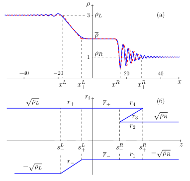
Figure 13: (a) Wave structure formed in the evolution of an initial discontinuity in the density distribution of a Bose condensate with $\rho_{L}=3$ and $\rho_{R}=1$, the evolution time being $t=10$. Solid line shows the numerical solution and the dashed line shows the analytic solution to the Gurevich-Pitaevskii problem. Theoretical values $\overline{\rho}=1.87$, $x_{-}^{L}/t=-1.73$, $x_{+}^{L}/t=-0.63$, $x_{-}^{R}/t=1.37$, $x_{+}^{R}/t=2.89$ agree well with the numerical solution. (b) Diagram of Riemann invariants corresponding to the wave structure formed in the evolution of the initial density discontinuity.

Just as in case of the KdV theory discussed in Section 7, we begin with the simplest problem of the evolution of the initial discontinuity, with the condensate state having different densities and different flow velocities, $\rho_{L},u_{L}$ and $\rho_{R},u_{R}$ , on the respective half-lines $x<0$ and $x>0$. The values of Riemann invariants are to be matched in the emerging wave structure, and we therefore specify the condensate state by their values on both sides of the discontinuity:

$$r_{\pm}(x,t)=\left\{\begin{array}[]{l}r_{\pm}^{L}=u_{L}/2\pm\sqrt{\rho_{L}},\quad x<0,\\ r_{\pm}^{R}=u_{R}/2\pm\sqrt{\rho_{R}},\quad x>0.\end{array}\right.$$ (215)

As an example, we consider the evolution of an initial discontinuity in the density distribution with the initial state $u_{L}=u_{R}=0$, and assume for definiteness that $\rho_{L}>\rho_{R}$, whence $r_{+}^{L}=-r_{-}^{L}>r_{+}^{R}=-r_{-}^{R}$.

The numerical solution of the Gross-Pitaevskii equation for this initial condition gives the wave structure shown with a solid line in Fig. 13(a). As we see, this structure consists of two waves joined by the domain of homogeneous flow (‘plateau’). Because parameters with the dimension of length are absent in the initial distribution, solutions of both dispersionless equations (192) and Whitham’s equations (204) must be self-similar and depend only on the variable $z=x/t$. Therefore, as can be easily verified, only one of the Riemann invariants can change along these waves. On the left, there is a rarefaction wave, along which the Riemann invariant $r_{+}$ is constant, i.e., $\sqrt{\rho_{L}}=\overline{u}/2+\sqrt{\overline{\rho}}$, where the bar over a variable denotes its value on the plateau. In the solution of Whitham’s equations, too, only one of the Riemann invariants $r_{i}$ varies, and we conclude that they can be matched continuously only if the Riemann invariant $r_{3}$ varies. The resultant wave structure can be represented by the diagram of the Riemann invariant shown in Fig. 13(b), which schematically shows the dependences of all the invariants on the self-similarity variable $z$. Because the invariant $r_{1}$ is constant along the DSW and matches the invariants $\overline{r}_{-}$ and $r_{-}^{R}$ on the DSW edges, we obtain one more equation $\overline{u}/2-\sqrt{\overline{\rho}}=-\sqrt{\rho_{R}}$ for the parameters of the flow along the plateau. The obtained equations determine the values of flow parameters on the plateau

$$\overline{\rho}=\frac{1}{4}(\sqrt{\rho_{L}}+\sqrt{\rho_{R}})^{2},\quad\overline{u}=\sqrt{\rho_{L}}-\sqrt{\rho_{R}}.$$ (216)

which are in excellent agreement with the numerical solution.

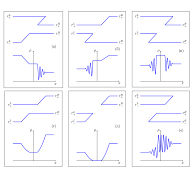
Figure 14: Wave structures formed in the evolution of the initial discontinuity in the theory of the Gross-Pitaevskii equation and the corresponding diagrams of Riemann invariants.

The above example shows that the shape of the wave structure resulting from the evolution of the initial discontinuity can be determined by joining pairs of Riemann invariant values corresponding to wave edges with lines having a positive slope and corresponding to self-similar solutions of the form $v_{i}=z$ (for the rarefaction wave, the positivity of the slope is obvious from expression (193) for characteristic dispersionless velocities, and for the DSW it follows from a more detailed investigation of expressions (207)). If there are only two Riemann invariants in the resultant domain, this domain corresponds to the rarefaction wave. If four invariants are defined in that domain, then it corresponds to the DSW.

It can be easily verified gk-87 ; eggk-95 that only six possible diagrams exist, which we present in Fig. 14 together with the corresponding wave structure types. In the cases shown in Fig. 14(a,b), one rarefaction wave and one DSW emerge, and these differ only in the wave propagation directions. In the case shown in Fig. 14(c) (‘collision of condensates’), two DSWs emerge on different sides of the plateau. In the cases in Fig. 14(d,e), the condensates on different sides of the discontinuity have opposite velocities and, as the condensates recede, a lower-density plateau appears between them; in Fig. 14(e), the initial velocities are so high that this density decreases to zero. Finally, in the case shown in Fig. 14(f), conversely, the head-on motion of the colliding condensates is so fast that, instead of a plateau, as in Fig. 14(c), a nonlinear periodic wave appears between the DSWs, with the $m$ parameter determined by the boundary values:

$$m=m^{*}=\frac{(r_{+}^{R}-r_{-}^{R})(r_{+}^{L}-r_{-}^{L})}{(r_{+}^{L}-r_{+}^{R})(r_{-}^{L}-r_{-}^{R})}.$$ (217)

So that just this combination of wave structures is realized, we must verify that the velocities of the rarefaction wave and DSW edges are ordered in a proper manner. This requires exploring the corresponding solutions of hydrodynamic and modulation equations.

A self-similar solution of Eqs. (192) with the required boundary conditions is not difficult to find. For example, for the rarefaction wave in Figs. 13 or 14(a), the Riemann invariant $r_{+}=u/2+\sqrt{\rho}=\sqrt{\rho_{L}}$ is constant, which defines the relation between $u$ and $\rho$ and in the simple wave. The first equation in (192) is satisfied, and the self-similar solution of the second equation has the form

$$v_{-}=\frac{1}{2}r_{+}+\frac{3}{2}r_{-}=\frac{3}{2}u-\sqrt{\rho_{L}}=z=\frac{x}{t}.$$

It readily follows from the obtained relations that

$$\rho=\frac{1}{9}\left(\sqrt{\rho_{L}}-\frac{2x}{t}\right)^{2},\quad u=\frac{2}{3}\left(\sqrt{\rho_{L}}+\frac{x}{t}\right).$$ (218)

The left edge of the rarefaction wave moves to the left with the speed of sound $s_{-}^{L}$, equal in modulus to $\sqrt{\rho_{L}}$, and the speed $s_{+}^{L}$ of the right edge can be found by equating one of the variables in (218) to its value (216) on the plateau, whence

$$s_{-}^{L}=-\sqrt{\rho_{L}},\quad s_{+}^{L}=\frac{1}{2}\sqrt{\rho_{L}}-\frac{3}{2}\sqrt{\rho_{R}}.$$ (219)

In the DSW in Fig. 13, the values of three Riemann invariants are known,

$$r_{1}=-\sqrt{\rho_{R}},\quad r_{2}=\sqrt{\rho_{R}},\quad r_{4}=\sqrt{\rho_{L}},$$ (220)

and the dependence of $r_{3}$ on $z=x/t$ is determined by the self-similar solution of Whitham’s equations:

$$v_{3}(-\sqrt{\rho_{R}},\sqrt{\rho_{R}},r_{3},\sqrt{\rho_{L}})=z=\frac{x}{t}.$$ (221)

Substituting all these values and the functions $r_{r}=r_{3}(z)$ into (202) gives the density profile in the DSW, which is shown with a dashed line in Fig. 13(a), in good agreement with the numerical solution. The velocities of the DSW edges can be found by substituting values (220) in the limit expressions (208) and (209) for $v_{3}$:

$$s_{-}^{R}=\frac{1}{2}(\sqrt{\rho_{L}}+\sqrt{\rho_{R}}),\quad s_{+}^{R}=\frac{2\rho_{L}-\rho_{R}}{\sqrt{\rho_{L}}}.$$ (222)

It is easy to verify that, for $\rho_{L}>\rho_{R}$, the velocities of the rarefaction wave and DSW edges are ordered in accordance with the inequalities $s_{-}^{L}<s_{+}^{L}<s_{-}^{R}<s_{+}^{R}$, in agreement with the diagram in Fig. 13(b).

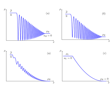
Figure 15: Transformation of a DSW as the density on the right boundary decreases. (a) Occurrence of avacuum point. (b) Vacuum point inside theDSW. (c) DSW with a small amplitude on the background of a rarefaction wave. (d) Transformation of the DSW into a rarefaction wave at zero density on the right boundary.

The soliton amplitude on the border with the plateau is

$$a_{s}=(r_{4}-r_{2})(r_{2}-r_{1})=2(\sqrt{\rho_{L}\rho_{R}}-\rho_{R}).$$ (223)

If we fix $\rho_{L}$ and decrease $\rho_{R}$ from its maximum value $\rho_{L}$ , we see that at $\rho_{R}=\rho_{L}/9$ the soliton depth $a_{s}$ becomes equal to the background density $\overline{\rho}$ defined on the plateau by expression (216). This means that this soliton becomes black, and the condensate density distribution acquires a ‘vacuum point’ gk-87 ; eggk-95 . As $\rho_{R}$ decreases further, the leading soliton amplitude becomes less than the background density, and the vacuum moves inwards the DSW. For the vanishing density $\rho_{R}$, the amplitude of oscillations in the DSW tends to zero together with soliton amplitude (223), the plateau disappears together with the left rarefaction wave, but the entire DSW domain becomes a rarefaction wave, Eq. (218), corresponding to the expansion of the condensate into the vacuum. This transformation of the DSW depending on the boundary conditions is illustrated in Fig. 15.

Other configurations shown in Fig. 14 can be considered similarly. It must only be kept in mind that, in Fig. 14(f), the modulated waves are matched not with the homogeneous flow on the plateau but with a non-modulated periodic solution with a known value (217) of the $m$ parameter.

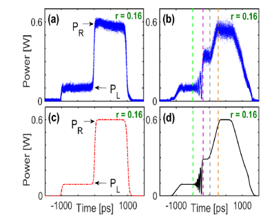
Figure 16: Intensity profiles measured (a) at the entrance to the optical fiber and (b) at the exit from it. (c) Initial condition and (d) the result of solving the NLS equation numerically with that initial condition. (From xckmt-17 .)

The theory expounded here was confirmed quantitatively in a dedicated experiment xckmt-17 , in which an optical pulse had an artificially produced discontinuity in the light intensity distribution and the evolution of the pulse was governed by the NLS equation, equivalent to the Gross-Pitaevskii equation. Figure 16(a), which is borrowed from that paper, shows the intensity profile of the pulse entering the optical fiber, and Figs. 16(b,d) show the pulse profile at the exit. Figures 16(a,b) show the results of measurements, and Figs. 16(c,e), the results of a numerical solution of the NLS equation. The initial pulse has the shape of two table tops with different heights placed next to each other without a gap, such that a discontinuity in intensity occurs in the center. Its evolution is the main subject of interest here, whereas the rarefaction waves emerging on the outer edges of the structure can be ignored. As we can see, the wave emerging in the center corresponds to the case in Fig. 14(b), and the velocities of the rarefaction wave and DSW edges agree well the theoretical values.

The problem of the evolution of a discontinuity, despite its simplicity, is being used in more realistic applications, such as DSW formation in a condensate flowing past an obstacle hakim-07 ; legk-09 , which allows explaining the result of the experiments in ea-07 , at least qualitatively. We also note that experiments with a nonlinear evolution of pulses in a more complicated geometry, both in the physics of condensates kgk-04 ; hoefer-06 and in nonlinear optics wjf-07 , also allow interpretations within that scheme. In Section 15, we illustrate the method with the solution to a simple problem on condensate motion under the action of a steadily moving piston hae-08 .

15 Piston problem

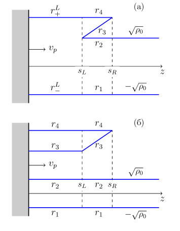
Figure 17: (a) Diagram of Riemann invariants in the problem of a piston for $v_{p}<2\sqrt{\rho_{0}}$. (b) Diagram of Riemann invariants for $v_{p}>2\sqrt{\rho_{0}}$.

We consider the problem of the flow of a condensate under the action of a piston hae-08 . We assume that the piston started moving at the instant $t=0$ with a constant velocity $v_{p}$ and that, prior to the motion of the piston, the condensate with a constant density $\rho_{0}$ was at rest to the right of the piston. It is clear that, as a result of that motion, a wave starts propagating from the piston; if the piston speed is not too high, it is natural to assume that adjacent to it is a homogeneous flow of the condensate with the same speed $v_{p}$ and with some increased density $\rho_{L}$. Between this homogeneous flow and the condensate at rest far from the piston, there is a DSW, and the values of Riemann invariants on the left and on the right of it can be expressed as

$$r_{\pm}^{L}=\frac{1}{2}v_{p}\pm\sqrt{\rho_{L}},\quad r_{\pm}^{R}=\pm\sqrt{\rho_{0}}.$$ (224)

The DSW originates instantaneously as the piston starts moving, and hence the solution of Whitham’s equations must be self-similar, and the diagram of Riemann invariants must have the form shown in Fig. 17(a). We use the equality $r_{-}^{L}=r_{1}=r_{-}^{R}$ to find the density $\rho_{L}$ of the flow adjacent to the piston:

$$\rho_{L}=\left(\frac{1}{2}v_{p}+\sqrt{\rho_{0}}\right)^{2},$$ (225)

This, in turn, determines the value of the Riemann invariant $r_{4}=r_{+}^{L}$. Hence, the values of three invariants that are constant along the DSW are known,

$$r_{1}=-\sqrt{\rho_{0}},\quad r_{2}=\sqrt{\rho_{0}},\quad r_{4}=v_{p}+\sqrt{\rho_{0}},$$ (226)

and the dependence of invariant $r_{3}$ on the self-similarity variable $z=x/t$ is defined implicitly by the equation

$$v_{3}(-\sqrt{\rho_{0}},\sqrt{\rho_{0}},r_{3},v_{p}+\sqrt{\rho_{0}})=z.$$ (227)

Using the limit expressions for $v_{3}$ in (208) and (209), we find the velocities of the DSW edges as

$$s_{L}=\frac{1}{2}v_{p}+\sqrt{\rho_{0}},\quad s_{R}=\frac{2v_{p}^{2}+4v_{p}\sqrt{\rho_{0}}+\rho_{0}}{v_{p}+\sqrt{\rho_{0}}}.$$ (228)

At the location of the deepest soliton adjacent to the homogeneous flow, formulas (195) and (196) give the minimal condensate density and the flow velocity:

$$\begin{split}&\rho_{\text{мин}}=\left(\sqrt{\rho_{0}}-\frac{1}{2}v_{p}\right)^{2},\\ &u_{\text{мин}}=-v_{p}\frac{\sqrt{\rho_{0}}+v_{p}/2}{\sqrt{\rho_{0}}-v_{p}/2}.\end{split}$$ (229)

For a sufficiently low piston speed, $v_{p}<2\sqrt{\rho_{0}}$, the flow velocity $u_{\text{мин}}$ is negative, and hence the condensate flows into the domain of increased density $\rho_{L}>\rho_{0}$, as expected.

For $v_{p}=2\sqrt{\rho_{0}}$, a vacuum point is formed in the DSW, with the velocity of the left DSW edge becoming equal to the piston speed, and hence the homogeneous flow domain adjacent to the piston disappears. For $v_{p}>2\sqrt{\rho_{0}}$, similarly to the case of the collision of condensates with too high velocities (Fig. 14(f)), the domain of a non-modulated periodic solution of the Gross-Pitaevskii equation occurs instead of the plateau, and this wave structure therefore corresponds to the diagram of Riemann invariants shown in Fig. 17(b). In the periodic wave, the Riemann invariants $r_{1},r_{2}$, $r_{4}$, preserve their values (226), and the condition that the wave velocity coincide with the piston speed $V=(r_{3}+r_{4})/2=v_{p}$ gives $r_{3}=v_{p}-\sqrt{\rho_{0}}$. Thus, in the periodic solution domain,

$$m^{*}=\frac{4\rho_{0}}{v_{p}^{2}}<1\quad\text{for}\quad v_{p}>2\sqrt{\rho_{0}},$$ (230)

and the condition of matching with the DSW determines the velocity of this DSW edge:

$$s_{L}=v_{p}+\frac{2\sqrt{\rho_{0}}(v_{p}-2\sqrt{\rho_{0}})K(m^{*})}{v_{p}E(m^{*})-(v_{p}-2\sqrt{\rho_{0}})K(m^{*})}.$$ (231)

The maximum density of the condensate in this structure is

$$\rho_{\text{max}}=(r_{4}-r_{3})(r_{2}-r_{1})=4\rho_{0}.$$ (232)

The density profile in the DSW can be constructed without difficulty by substituting the Riemann invariants in (202), and the analytic results agree well with numerical computations hae-08

The Gurevich-Pitaevskii method thus allows completely solving the problem posed in this section.

16 Uniformly accelerated piston problem

As in the case of the KdV equation, there are two scenarios for a simple wave breaking: the profile of one of dispersionless Riemann invariants $r_{\pm}$ acquires a vertical tangent either at the interface with the condensate, which is at rest, or at the inflection point. We here consider the first case and assume for definiteness that this profile is produced by a uniformly accelerated moving piston kk-10 , such that, at a time $t$, the coordinate of the condensate-piston boundary is $X(t)=at^{2}/2$.

Prior to the instant of breaking, the condensate flow can be described by dispersionless equations (192) with good accuracy, and we now give their solution in the form that we need. Under the action of the piston, the condensate flow is unidirectional and hence can be described by a simple wave with a constant Riemann invariant, $r_{-}=u/2-\sqrt{\rho}=-\sqrt{\rho_{0}}$, where $\rho_{0}$ is the initial density of the condensate in the domain that has not yet been reached by the wave produced by the piston. The invariant $r_{+}$ satisfies the first equation in (192); the general solution $x-(\frac{3}{2}r_{+}-\sqrt{\rho_{0}})t=w(r_{+})$ of that equation must satisfy the boundary condition $u(X(t),t)=\dot{X}(t)$, which states that the flow velocity on the boundary with the piston coincides with the piston velocity. Therefore, $r_{+}-\sqrt{\rho_{0}}=at$, and using the general solution for the condensate flow on the boundary with the piston gives $w=at^{2}/2-(\frac{3}{2}r_{+}-\sqrt{\rho_{0}})t$. After eliminating $t=(r_{+}-\sqrt{\rho_{0}})/a$, we obtain the general solution for the condensate flow in the form

$$x-\left(\frac{3}{2}r_{+}-\frac{1}{2}\sqrt{\rho_{0}}\right)t=\frac{1}{a}\sqrt{\rho_{0}}r_{+}-\frac{1}{a}r_{+}^{2}.$$ (233)

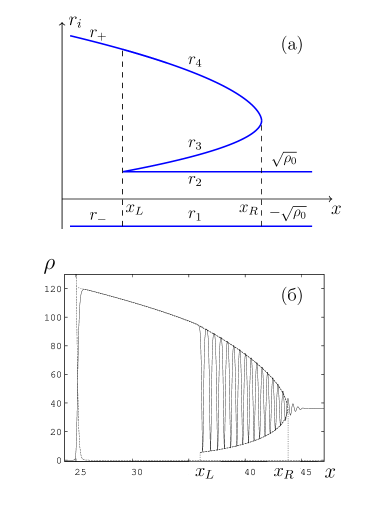
Figure 18: (a) Diagram of Riemann invariants in the problem of a uniformly accelerated piston. (b) Density profile in the condensate moving under the action of a uniformly accelerated piston. Solid line shows the numerical computation result and the dashed line shows the envelope, in accordance with the analytic theory.

This solution holds in the entire inhomogeneous flow domain until the instant $t_{b}={2\sqrt{\rho_{0}}}/(3a)$ when the $r_{+}(x)$ profile acquires a vertical tangent at the point $x_{b}={2\rho_{0}}/(3a)$ on the boundary with the condensate at rest. After that instant of breaking, a wave structure involving a DSW emerges, with the distribution of Riemann invariants represented by the diagram shown in Fig. 18(a). We therefore have to find a solution of Whitham’s equations with the constant Riemann invariants $r_{1}=-\sqrt{\rho_{0}}$ and $r_{2}=\sqrt{\rho_{0}}$, a solution satisfying the condition that $r_{4}$ match the invariant $r_{+}$ of dispersionless solution (233) as $r_{3}\to r_{2}$. The right-hand side of (233) contains linear and quadratic terms in $r_{+}$. As in the KdV problems considered above, it suffices to take a linear combination of the expressions $w_{i}^{(1)}\equiv v_{i}$ and $w_{i}^{(2)}$ that has just that dependence in the limit as $r_{3}\to r_{2}$. The coefficients of this linear combination are chosen from the condition of matching $r_{4}$ with $r_{+}$, and a straightforward calculation kk-10 yields a solution in the form

$$\begin{split}x-v_{3}(r)t=\frac{2}{5a}\left(\rho_{0}+\sqrt{\rho_{0}}v_{3}(r)-\frac{8}{3}w_{3}^{(2)}(r)\right),\\ x-v_{4}(r)t=\frac{2}{5a}\left(\rho_{0}+\sqrt{\rho_{0}}v_{4}(r)-\frac{8}{3}w_{4}^{(2)}(r)\right).\end{split}$$ (234)

These formulas implicitly define the dependences of $r_{3}$and $r_{4}$ on $x$ and $t$, and their substitution in (202) gives the DSW density profile, whose envelope is compared in Fig. 18(b) with the results of a numerical solution of the Gross-Pitaevskii equation.

Importantly, formulas (234) allow finding the main DSW parameters analytically. For example, in the soliton limit $r_{3}=r_{2}$, the difference between these formulas on the boundary $x=x_{L}(t)$ gives the time dependence of $r_{4}$ in the form $r_{4}=5at/4+\sqrt{\rho_{0}}/6$, substituting which in any of formulas (234) leads to the law of motion of the soliton edge of the DSW:

$$x_{L}(t)=\frac{5}{36}\frac{\rho_{0}}{a}+\frac{7}{12}\sqrt{\rho_{0}}\,t+\frac{5}{16}at^{2}.$$ (235)

In the small-amplitude limit $r_{3}=r_{4}$, Eqs.(234) reduce to a single equation on the boundary $x=x_{R}(t)$:

$$x-\frac{2r_{4}^{2}-\rho_{0}}{r_{4}}t=\frac{2}{5a}\left(3\rho_{0}+2\sqrt{\rho_{0}}r_{4}-\frac{\rho_{0}^{3/2}}{r_{4}}-4r_{4}^{2}\right),$$

with the boundary value $x_{R}$ corresponding to the maximum of this function $x(r_{4})$ at a fixed value of $t$. This implies the dependence of $t$ on $y=r_{R}/\sqrt{\rho_{0}}$:

$$t=\frac{2\sqrt{\rho_{0}}}{5a}\cdot\frac{8y^{3}-2y^{2}-1}{2y^{2}+1},\quad y\geq 1,$$ (236)

substituting which in the limit expression for (234) gives

$$x_{R}=\frac{2\rho_{0}}{5a}\cdot\frac{8y^{4}-6y^{2}+3}{2y^{2}+1},$$ (237)

The obtained formulas define the law of motion of the small- amplitude DSW edge in parametric form. At $t=t_{b}$ ($y=1$), the coordinates of both edges are equal to the breaking point coordinate $x_{b}$, in accordance with the fact that in the asymptotic Gurevich-Pitaevskii approach the DSW has a vanishing length at the instant of formation. The derived laws of motion for the DSW edges agree well with numerical solutions of the Gross-Pitaevskii equation kk-10 . The solution to the breaking problem for a simple wave expanding into a medium at rest and having a power-law profile $r_{+}\propto(-x)^{1/n}$ at the instant of breaking can be found similarly for any integer $n$ (see kamch-18a ).

17 Motion of edges of ‘quasi-simple’ dispersive shock waves

A characteristic feature of a wave formed in the condensate as a result of the motion of a piston was that it expanded into the depth of the condensate at rest, and therefore in the DSW domain two out of the four Riemann invariants of Whitham’s system were constant, and only the other two changed in the course of evolution. This is similar to the KdV case considered in Section §10, where one invariant was constant and two others were variable. In gkm-89 , DSWs of this type were called ‘quasi-simple’. The law of motion of their edges can again be found in the theory of the Gross-Pitaevskii equation following a strategy similar to that presented in Section §10. In view of a close analogy with Section §10, we here give only the basic facts of the corresponding theory kamch-19 ; kamch-20 .

For definiteness, we consider the breaking of a simple wave for which the invariant $r_{-}=u/2-c=-c_{0}$ is constant, where $c=\sqrt{\rho}$ is the local speed of sound, which takes the value $c_{0}=\sqrt{\rho_{0}}$ in the unperturbed domain of the condensate. We then have $r_{+}=u/2+c=2c-c_{0}$ and $v_{+}=3c-2c_{0}$, and the solution of dispersionless equations (192) can be written as

$$x-(3c-2c_{0})t={\overline{x}}(c-c_{0}),$$ (238)

where ${\overline{x}}(c-c_{0})$ is a function inverse to the initial distribution $c-c_{0}=w(x)$ at the instant of breaking $t=0$. We first assume that the initial pulse is ‘positive,’ i.e., $c-c_{0}>0$. This solution borders the soliton edge of the DSW, which moves with the soliton velocity $V_{s}=(r_{4}+r_{2})=c$, where we used the fact that $r_{2}=-r_{1}=c_{0}$ along the quasi-simple DSW and $r_{4}=r_{+}=2c-c_{0}$ at the matching point. Therefore, $dx_{L}-cdt=0$ and dispersionless solution (238) on the boundary with the DSW for $x=x_{L}$ must be compatible with the equation

$$\frac{dx_{L}}{dc}-c\frac{dt}{dc}=0,$$ (239)

where $x_{L}$ and $t$ are regarded as functions of the local speed of sound $c$, which varies on the soliton edge as a result of the DSW evolution. After eliminating $x_{L}$, we hence obtain the equation

$$2z\frac{dt}{dc}+3t=-\frac{d{\overline{x}}}{dc},\quad z=c-c_{0},$$ (240)

solving which with the initial condition $t(0)=0$,

$$t(z)=-\frac{1}{2z^{3/2}}\int_{0}^{z}\sqrt{z}\,{\overline{x}}^{\prime}(z)dz,$$ (241)

together with the equation

$$x_{L}(z)=(3z+c_{0})t(z)+{\overline{x}}(z)$$ (242)

defines the law of motion of the soliton DSW edge over a monotonic dispersionless profile in parametric form.

If the profile is not monotonic and has a maximum $c_{m}=c_{0}+z_{m}$, then, for $t>t_{m}=t(z_{m})$, when the soliton edge borders the branch ${\overline{x}}_{2}(c-c_{0})$ of the dispersionless solution, instead of (241) and (242) we easily find the relations

$$\begin{split}&t(c)=-\frac{1}{2(c-c_{0})^{3/2}}\int_{0}^{{\overline{x}}_{2}(c-c_{0})}\sqrt{\widetilde{c}_{0}(x)}dx,\\ &x_{L}(c)=(3c-2c_{0})t(c)+{\overline{x}}_{2}(c),\end{split}$$ (243)

where $c_{0}+\widetilde{c}_{0}(x)$ is the initial distribution of the local speed of sound. At asymptotically large times, we hence find

$$x_{L}=c_{0}t+3\left(\frac{\mathcal{A}}{2}\right)^{2/3}t^{1/3},\quad\mathcal{A}=\int_{-\infty}^{0}\sqrt{\widetilde{c}_{0}(x)}\,dx.$$ (244)

In this asymptotic limit, the DSW amplitude becomes much less than the background density $\rho_{0}$, and the Gross-Pitaevskii equation can be approximated for unidirectional wave propagation with the KdV equation; hence, solution (244) coincides with (151) in the corresponding variables.

On the low-amplitude edge, in the same asymptotic regime, $r_{3}\approx r_{4}\approx r_{m}=2c_{m}-c_{0}$ and $r_{2}=-r_{1}=c_{0}$, and therefore formula (205) gives the wavelength

$$L=\frac{\pi}{2\sqrt{c_{m}(c_{m}-c_{0})}}$$

and the wave number $k=4\sqrt{c_{m}(c_{m}-c_{0})}$. Hence, the group velocity of motion of the small-amplitude edge is

$$\frac{dx_{R}}{dt}=\left.\frac{d\omega}{dk}\right|_{k=k_{m}}=2r_{m}-\frac{c_{0}^{2}}{r_{m}}.$$ (245)

In the case of a negative initial pulse with $\widetilde{c}_{0}(x)=c-c_{0}<0$, similarly, the small-amplitude edge borders the dispersionless solution (238), with the Riemann invariants of Whitham’s system given by $r_{3}=r_{4}=-r_{1}=c_{0}$ and $r_{2}=2c-c_{0}$, where $c$ is the local speed of sound on that edge. Therefore, the wavelength is here given by $L=\pi/(2\sqrt{c_{0}(c_{0}-c)})$, i.e. $k=4\sqrt{c_{0}(c_{0}-c)}$, and this edge moves over the background with the parameters $\rho=c^{2}$, $u=2(c-c_{0})$ with the group velocity

$$\frac{dx_{R}}{dt}=\frac{d\omega}{dk}=u+\frac{c^{2}+k^{2}/2}{\sqrt{c^{2}+k^{2}/4}}=2c_{0}-\frac{c^{2}}{2c_{0}-c}.$$ (246)

The compatibility condition of Eq. (238) with the equation

$$\frac{dx_{R}}{dc}-\left(2c_{0}-\frac{c^{2}}{2c_{0}-c}\right)\frac{dt}{dc}=0$$ (247)

leads to the differential equation

$$\frac{(4c_{0}-c)(c_{0}-c)}{2c_{0}-c}\frac{dt}{dc}-\frac{3}{2}t=\frac{1}{2}{\overline{x}}^{\prime}(c-c_{0}),$$

whose solution gives a parametric law of motion of the right DSW edge

$$\begin{split}&t(c)=\frac{1}{2(4c_{0}-c)\sqrt{c_{0}-c}}\int_{c_{0}}^{c}\frac{(2c_{0}-c){\overline{x}}^{\prime}(c-c_{0})}{\sqrt{c_{0}-c}}dc,\\ &x_{R}(c)=(3c-2c_{0})t(c)+{\overline{x}}(c).\end{split}$$ (248)

It is easy to rewrite it, with obvious changes, for localized pulses with a single local minimum.

In the case of a negative initial pulse, the asymptotic state mainly consists of dark solitons, and it is easy to find the velocity of the deepest soliton on the left DSW edge. We here have $r_{4}=-r_{1}=c_{0}$ and $r_{2}\approx r_{3}\approx r_{m}=2c_{m}-c_{0}$, whence

$$\frac{dx_{L}}{dt}=\frac{1}{2}\sum r_{i}\approx r_{m}=2c_{m}-c_{0}.$$ (249)

The number of dark solitons into which the initial negative pulse eventually decays can be found following the same strategy that we used to derive Karpman’s formula (159) for the KdV equation. On the small-amplitude edge, we now have $k(v_{g}-V)=k^{3}/(4\sqrt{c^{2}+k^{2}/4})$ and $k=4\sqrt{c_{0}(c_{0}-c)}$. Substituting these expressions into the general formula (155) and using (248) to replace the integration over $t$ with integration over $c$, after simple transformations we obtain

$$N=\frac{2}{\pi}\int\sqrt{c_{0}(c_{0}-c(x))}\,dx,$$ (250)

where $c(x)$ is the initial distribution of the local speed of sound in the wave. The Gross-Pitaevskii equation, just like the KdV equation, is completely integrable, making the inverse scattering transform method zs-73 applicable to it, which allows finding jlml-99 ; kku-02 the general expression for the number of solitons originating from the pulse with the given initial distributions of dispersionless Riemann invariant $r_{\pm}(x)$:

$$N=\frac{1}{\pi}\int\sqrt{(c_{0}-r_{-}(x))(c_{0}-r_{+}(x))}\,dx.$$ (251)

In our case of the evolution of the pulse in the form of a simple wave, $r_{-}(x)=-c_{0}$ and $r_{+}(x)=2c(x)-c_{0}$, and formula (251) reduces to (250). We must note, however, that both formula (159) for the KdV equation and formula (250) for the Gross-Pitaevskii equation can be represented as

$$N=\frac{1}{2\pi}\int k_{0}(x)dx,$$ (252)

where $k_{0}(x)$ is the wave number on the small-amplitude edge corresponding to the initial distribution of the parameters of the simple wave. Formula (252) apparently is of a general nature and can also be applied to equations that are not completely integrable egkkk-07 ; egs-08 , for which the dependence $k_{0}(x)$ is to be found by solving equation for the conservation of the number of waves along the trajectory of the small-amplitude edge te-99 ; el-05 .

18 Breaking of a cubic profile in the Gross-Pitaevskii theory

In the general case, a wave governed by the Gross-Pitaevskii equation breaks in such a way that the profile of one of the dispersionless Riemann invariants $r_{\pm}$ acquires a vertical tangent and can be approximately represented by a cubic curve near the inflection point. We assume for definiteness that the invariant $r_{+}$ undergoes breaking, and it hence varies in the neighborhood of that point very rapidly, which allows assuming the $r_{-}$ invariant to be constant. By an appropriate change of variables, it can be ensured that the condensate flow is described by the formulas

$$x-\left(\frac{3}{2}r_{+}+\frac{1}{2}r_{-}^{0}\right)t=-r_{+}^{3},\quad r_{-}=r_{-}^{0}=\mathrm{const},$$ (253)

up to the instant of breaking. These formulas give a solution of hydrodynamic equations (192). Naturally, it is assumed here that $r_{-}^{0}<r_{+}$ in the domain of interest, including the solution branch in (253) with $r_{+}<0$. For $t>0$, solution (253) becomes multi-valued. Taking dispersion into account, i.e., solving the full Gross-Pitaevskii equation, eliminates this multi-valuedness by the formation of a DSW. Following the Gurevich-Pitaevskii approach, we solve this problem kku-02 ; kk-10 in Whitham’s approximation by incorporating the solution of Whitham’s equations in dispersionless solution (253) such that the equality $r_{1}=r_{-}^{0}$ holds and the boundary conditions

$$\begin{split}&r_{4}(x_{L}(t),t)=r_{+}(x_{L}(t),t)\quad\text{при}\quad r_{3}=r_{2},\\ &r_{2}(x_{R}(t),t)=r_{+}(x_{R}(t),t)\quad\text{при}\quad r_{3}=r_{4}.\end{split}$$ (254)

are satisfied. Because the right-hand side of the first equation in (253) involves a cubic function of $r_{3}$, we can satisfy all the conditions by taking solution (210) with $r_{1}=r_{-}^{0}$ and $w_{i}=\sum_{k=0}^{3}A_{k}w_{i}^{(k)}$ are given by formulas (213) and (214) and the coefficients $A_{k}$ are chosen such that the matching conditions are satisfied. As a result, we obtain

$$\begin{split}&x-v_{i}(r)t=-\tfrac{32}{35}{w_{i}^{(3)}}(r)+\tfrac{16}{35}{w_{i}^{(2)}}(r)r_{-}^{0}+\\ &+\tfrac{2}{35}{v_{i}}(r)(r_{-}^{0})^{2}+\tfrac{1}{35}(r_{-}^{0})^{3},\quad i=2,3,4,\end{split}$$ (255)

These formulas implicitly define the dependence of the invariants $r_{2},r_{3}$, and $r_{4}$ on $x$ and $t$. In particular, investigating the limit $r_{3}\to r_{3}$, we can easily find the law of motion of the soliton edge of the DSW:

$$x_{L}(t)=\frac{1}{2}r_{-}^{0}t-\frac{1}{6}\sqrt{\frac{5}{3}}\,t^{3/2}.$$ (256)

The law of motion of the small-amplitude edge

$$x_{R}=\left(\frac{3}{2}r_{2}+\frac{1}{2}r_{-}^{0}\right)t(r_{2},r_{4})-r_{2}^{3}$$ (257)

is defined in parametric form, with the time $t$ depending on the parameters $r_{2}$ and $r_{4}$ as

$$t=\frac{2[8(r_{4}-7r_{-}^{0})(3r_{2}^{2}+4r_{2}r_{4}+8r_{4}^{2})-15r_{2}^{3}]}{35(4r_{4}-r_{2}-3r_{-}^{0})},$$ (258)

and the parameters themselves related as

$$\begin{split}&21(r_{-}^{0})^{2}(4r_{4}+r_{2})-10r_{-}^{0}(20r_{4}^{2}+2r_{2}r_{4}+r_{2}^{2})+\\ &+16r_{4}(8r_{4}^{2}-r_{2}r_{4}-r_{2}^{2})+9r_{2}^{3}=0.\end{split}$$ (259)

We see that this particular Gurevich-Pitaevskii problem has also been given a fully analytic solution.

19 Conclusions

We have presented the Gurevich-Pitaevskii theory for DSWs in some detail following gp-73 and other closely related papers. It remains to briefly mention some avenues of further development of this theory.

We first note that, simultaneously with the appearance and development of the theory of DSWs, other important events were taking place in nonlinear physics associated with the discovery of the inverse scattering transform method for solutions of nonlinear wave equations ggkm-67 ; lax-68 ; zs-73 . A fundamental fact of that method is the relation between the so-called completely integrable equations, a class to which the KdV and Gross-Pitaevskii equations belong, and the associated linear spectral problems. For example, associated with the KdV equation is the problem of the spectrum of a quantum particle moving in the potential $u(x,t)$; the relation is such that, in particular, the parameters of the soliton solution are related to the discrete spectrum of that potential.

An extension of this method to periodic solutions of the KdV equation nov-74 ; dmn-76 has shown that the Riemann invariants of Whitham’s system coincide with the endpoints of gaps where the motion of the quantum particle is forbidden in the corresponding periodic potential. This allowed, on the one hand, generalizing the Whitham method to multi-phase solutions ffm-80 and, on the other hand, extending it to other integrable equations. In particular, we have used Whitham’s equations for the Gross-Pitaevskii theory, which were found in FL-86 ; pavlov-87 by methods based on the complete integrability of that equation.

It turns out as a result that three sets of parameters characterizing the periodic solutions arise naturally in the theory: (1) physical parameters $\nu_{i}$ related to the wave amplitude and other quantities that bear a clear physical meaning; (2) the end points $\lambda_{i}$ of the periodic spectral problem; (3) the Riemann invariants $r_{i}$ of Whitham’s modulation system for the considered periodic wave.

In the simplest case of the KdV equation, the relations among all these parameters are linear, and this is why Whitham could diagonalize the modulation equations derived for physical parameters by choosing appropriate linear combinations. In the case of the Gross-Pitaevskii equation, the relation between $\lambda_{i}$ and $r_{i}$ remains linear, and that is why we were able to not invoke $\lambda_{i}$ in our presentation, but the physical parameters $\nu_{i}$ are related to $r_{i}$ (or $\lambda_{i}$) by more complicated formulas (201). This complication, technical at first glance, becomes fundamentally important when the relation between $\lambda_{i}$ and $r_{i}$ becomes multi-valued: one solution of Whitham’s equations corresponds to two different periodic waves. This situation is characteristic of the so-called not genuinely nonlinear equations, in which nonlinear terms can vanish for some amplitude of the wave. This was noted in pt-06 for a higher KdV equation, an element of a hierarchy of equationsas sociated with the samespectral problem, and also in marchant-08 for the modified KdV equation $u_{t}\pm 6u^{2}u_{x}+u_{xxx}=0$, where the coefficient in the nonlinear term has a maximum or a minimum at $u=0$, depending on the sign.

In the problem of the evolution of a step-like profile, this led to the appearance of more complicated structures than rarefaction waves and modulated cnoidal waves that we are familiar with from the theory outlined in the foregoing. A classification of such structures evolving from the initial discontinuity in accordance with the Gardner equation $u_{t}+6(u\pm\alpha u^{2})u_{x}+u_{xxx}=0$ that occurs in the theory of internal water waves was given in kamch-12 . In the theory of the modified NLS equation $i\psi_{t}+\tfrac{1}{2}\psi_{xx}-i(|\psi|^{2}\psi)_{x}=0$, which has applications in nonlinear optics and magnetohydrodynamic waves, the use of all three sets of parameters becomes necessary: periodic solutions and Whitham’s equations were obtained in kamch-90 , and the evolution of the initial discontinuity was analyzed in gke-92b ; ik-17 ; kamch-18 . Finally, the most complicated case of this type, a ferromagnet with ‘easy plane’ anisotropy and the equivalent limit for two-component Gross-Pitaevskii equations, was studied in kamch-92 ; ikcp-17 .

Besides the development of Whitham’s averaging method, the discovery of the complete integrability of the most important equations in nonlinear wave physics has allowed developing other approaches to the theory of DSWs. In particular, it was shown in ll-83a ; ll-83b ; ll-83c ; ven-85a ; ven-85b ; mazur-96 that the solution to the Gurevich-Pitaevskii problem in Whitham’s approximation can also be obtained as a semiclassical limit of exact multi-soliton solutions of the KdV equation. Another aspect of a more exact theory of DSWs is that, similarly to how the linear problem solution (25) obtained by the averaging method is an asymptotic form of the Airy function, Whitham’s approximation for breaking waves is a semiclassical asymptotic form of some special functions that are ‘standard’ solutions of the Painlevé nonlinear differential equations (see, e.g., sul-94 ; gs-10 ; cg-10 ). Solutions expressed in terms of such special functions are also exact at the small-amplitude edge of the DSW.

Another area of investigations is to generalize the Gurevich-Pitaevskii approach to equations that are not completely integrable. Naturally, the Whitham theory considered above for the perturbed KdV equation can be generalized to a rather wide class of equations close to completely integrable ones kamch-04 ; lkp-12 . However, a large number of physically important equations do not fall into that category and the modulation equations for periodic solutions of such equations do not have Riemann invariants in any approximation. Still, the general Gurevich-Pitaevskii approach is also valid for them and some important characteristic of DSWs can be calculated with no Riemann invariants defined.

The first important statement regarding such systems, made by Gurevich and Meshcherkin gm-84 , was that only a DSW is formed in the breaking of a simple wave, and the constant Riemann invariant of the dispersionless limit transports its value across the DSW, despite the absence of Whitham’s Riemann invariant conserved along the DSW. This statement is already sufficient in order to calculate the parameters of the plateau appearing between two wave structures in the evolution of a discontinuity.

The next important step was made in te-99 ; el-05 , where it was noted that, on the border with a simple wave, Whitham’s system reduces to an ordinary differential equation whose solution gives a relation between the DSW parameters on that edge. Because one of the modulation equations (the conservation law for the number of waves) is certainly known on the small-amplitude edge, the solution of that equation gives a relation between the wave number and the background amplitude of the wave. On the soliton edge, such an equation is absent in general. But it can be verified that, in the case of KdV and Gross-Pitaevskii equations, the equation $\widetilde{k}_{t}+\widetilde{\omega}_{x}=0$ holds for pulse expansion into a medium at rest with two constant Riemann invariants, with $\widetilde{k}$ being the inverse half-width of the soliton and $\widetilde{\omega}(\widetilde{k})$ obtained from the linear dispersion law $\omega(k)$ by the substitution $\widetilde{\omega}(\widetilde{k})=-i\omega(i\widetilde{k})$. According to an old remark by Stokes quoted in a note to §252 in lamb , $\widetilde{\omega}(\widetilde{k})$ determines the soliton velocity: the tails of the soliton propagate with the same velocity as the soliton itself, and on the tails the linearized equations have the same form as in the small-amplitude harmonic limit.

Assuming the validity of the equation $\widetilde{k}_{t}+\widetilde{\omega}_{x}=0$ in the general case of the breaking of simple waves expanding into a ‘quiescent’ homogeneous medium with two constant dispersionless Riemann invariants, we can obtain an ordinary differential equation for the parameters along the soliton edge of the DSW. These two equations are entirely sufficient for finding the parameters of the edges of the DSW forming in the evolution of a discontinuity and satisfying an unintegrable equation, as was indeed done in series of studies el-05 ; egs-06 ; egkkk-07 ; ep-11 ; lh-13 ; hoefer-14 ; ckp-16 ; hek-17 ; ams-18 . Requiring the compatibility of the thus obtained ordinary differential equation with the solution of the dispersionless equations on that boundary allows obtaining the equation of motion for the DSW edge propagating over the general profile of a simple wave kamch-19 ; ik-19 ; kamch-20 .

A new type of DSW can occur when taking higher-order dispersion effects into account when the soliton velocity is equal to the phase velocity of linear waves and these are in resonance with other. The general Gurevich-Pitaevskii approach is also applicable in that case smyth-16 ; es-16 ; hss-18 ; bs-20 .

In this paper, we mentioned applications of the Gurevich-Pitaevskii problem to water waves, plasmas, Bose-Einstein condensate, and nonlinear optics. To these, we can add the observations and the theory of DSWs in internal waves in the ocean hm-06 and the atmosphere ps-02 , and on jets of a liquid in viscous media maiden-16 ; maiden-20 . The Gurevich-Pitaevskii approach to the DSW theory also extends to waves with several spatial variables abr-18 and finds applications in other areas in physics, including the quantum gravity theory sul-94 . The reader can find more examples of DSWs, e.g., in review eh-16 and the references therein. In addition, the creation of the DSW theory was related to the substantial progress in modern mathematical physics, and the reader can glean some aspects of the mathematical theory from reviews dm-80 ; dn-89 .

To conclude, we can say that in the years that have passed since the appearance of paper gp-73 , the Gurevich-Pitaevskii problem, understood as a general approach to the DSW theory based on Whitham’s modulation equations, has become an area of vibrant research in nonlinear physics, with a distinctive problem setting and with profound mathematical methods for solving problems and clear physical ideas that enrich the entire physics of nonlinear waves.

I am grateful to L. P. Pitaevskii for discussions of the problems considered in this paper and for his useful remarks.

References

- (1) Gurevich A V, Pitaevskii L P Sov. Phys. JETP 38 291 (1974); Zh. Eksp. Teor. Fiz. 65 590 (1973)
- (2) Whitham G B Proc. Roy. Soc. London 283 238 (1965)
- (3) Scott Russel J Report on waves (British Association Reports, 1844).
- (4) Boussinesq J Comptes Rendus 72 755 (1871)
- (5) Lord Rayleigh Phil. Mag. 1 257 (1876)
- (6) Korteweg D J, de Vries G Phil. Mag. 39 422 (1895)
- (7) Benjamin T B, Lighthill M J Proc. Roy. Soc. Lond. A 224 448 (1954)
- (8) Lamb H Hydrodynamics (Cambridge: Cambridge Univ. Press, 1932)
- (9) Stoker J J Water Waves; the Mathematical Theory with Applications (New York: Interscience Publ., 1957)
- (10) Gardner S C, Morikawa G K, “Similarity in the asymptotic behavior of collision-free hydromagnetic waves and water waves”, Courant Institute of Mathematical Sciences Report No. NYO‐9082 (N. Y. 1960)
- (11) Vedenov A A, Velikhov E P, Sagdeev R Z Nucl. Fusion 1 82 (1961); Yad. Sintez 1 82 (1961)
- (12) Sagdeev R Z, in Reviews of Plasma Physics Vol. 4 (Ed. M A Leontovich) (New York: Consultants Bureau, 1966) p. 23; Translated from Russian: in Voprosy Teorii Plazmy Issue 4 (Ed. M A Leontovich) (Moscow: Gosatomizdat, 1964) p. 20
- (13) Alikhanov S G, Belan V G, Sagdeev R Z JETP Lett. 7 318 (1968); Pis’ma Zh. Eksp. Teor. Fiz. 7 405 (1968)
- (14) Taylor R J, Baker D R, Ikezi H, Phys. Rev. Lett. 24 206 (1970)
- (15) Gurevich A V, Pariiskaya L V, Pitaevskii L P Sov. Phys. JETP 22 449 (1966); Zh. Eksp. Teor. Fiz. 49 647 (1965)
- (16) Gurevich A V, Pariiskaya L V, Pitaevskii L P Sov. Phys. JETP 27 476 (1968); Zh. Eksp. Teor. Fiz. 54 891 (1968)
- (17) Gurevich A V, Pitaevskii L P Sov. Phys. JETP 29 954 (1969); Zh. Eksp. Teor. Fiz. 56 1178 (1969)
- (18) Gurevich A V, Pitaevskii L P Sov. Phys. JETP 33 1159 (1971); Zh. Eksp. Teor. Fiz. 60 2155 (1971)
- (19) Lifshitz E M, Pitaevskii L P Physical Kinetics (Oxford: Pergamon Press, 1981); Translated from Russian: Fizicheskaya Kinetika (Moscow: Fizmatlit, 2001)
- (20) Abramowitz M, Stegun I A (Eds) Handbook of Mathematical Functions with Formulas, Graphs, and Mathematical Tables (New York: Dover Publ., 1972)
- (21) Whitham G B Linear and Nonlinear Waves (New York: Wiley, 1974)
- (22) Landau L D, Lifshitz E M Fluid Mechanics (Oxford: Pergamon Press, 1987); Translated from Russian: Gidrodinamika (Moscow: Fizmatlit, 2001)
- (23) Rozdestvenskii B L, Janenko N N Systems of Quasilinear Equations and Their Applications to Gas Dynamics (Providence, RI: American Mathematical Society, 1983); Translated from Russian: Sistemy Kvazilineinykh Uravnenii i Ikh Prilozheniya k Gazovoi Dinamike (Moscow: Nauka, 1978)
- (24) Gardner S C et al. Phys. Rev. Lett. 19 1095 (1967)
- (25) Gurevich A V, Krylov A L, Mazur N G Sov. Phys. JETP 68 966 (1989); Zh. Eksp. Teor. Fiz. 95 1674 (1989)
- (26) Gurevich A V, Krylov A L, El’ G A JETP Lett. 54 102 (1991); Pis’ma Zh. Eksp. Teor. Fiz. 54 104 (1991)
- (27) Gurevich A V et al. Sov. Phys. Dokl. 37 198 (1992); Dokl. Ross. Akad. Nauk 323 876 (1992)
- (28) Gurevich A V, Krylov A L, El’ G A Sov. Phys. JETP 74 957 (1992); Zh. Eksp. Teor. Fiz. 101 1797 (1992)
- (29) El G A, Khodorovsky V V Phys. Lett. A 182 49 (1993)
- (30) Kudashev V P, Sharapov S E Theor. Math. Phys. 85 1155 (1990); Teor. Matem. Fiz. 85 205 (1990)
- (31) Kudashev V P, Sharapov S E Theor. Math. Phys. 87 358 (1991); Teor. Matem. Fiz. 87 40 (1991)
- (32) Kudashev V R Phys. Lett. A 166 213 (1992)
- (33) Kudashev V R Phys. Lett. A 171 335 (1992)
- (34) Wright O C Commun. Pure Appl. Math. 46 423 (1993)
- (35) Tian F R Commun. Pure Appl. Math. 46 1093 (1993)
- (36) Tsarev S P Sov. Math. Dokl. 31 488 (1985); Dokl. Akad. Nauk SSSR 282 534 (1985)
- (37) Grimshaw R H J, Smyth N J Fluid Mech. 169 429 (1986)
- (38) Smyth N Pros. Roy. Soc. Lond. A 409 79 (1987)
- (39) Potëmin G V Russ. Math. Surv. 43 252 (1988); Usp. Matem. Nauk 43 211 (1988)
- (40) Kamchatnov A M Phys. Rev. E 99 012203 (2019)
- (41) Gurevich A V, Pitaevskii L P Sov. Phys. JETP 66 490 (1987); Zh. Eksp. Teor. Fiz. 93 871 (1987)
- (42) Karpman V I Phys. Lett. A 25 708 (1967)
- (43) Deift P, Venakides S, Zhou Z Commun. Pure Appl. Math. 47 199 (1994)
- (44) Isoard M, Kamchatnov A M, Pavloff N Phys. Rev. E 99 012210 (2019)
- (45) Avilov V V, Krichever I M, Novikov S P Sov. Phys. Dokl. 32 564 (1987); Dokl. Akad. Nauk SSSR 295 345 (1987)
- (46) Gurevich A V, Pitaevskii L P Sov. Phys. JETP 72 821 (1991); Zh. Eksp. Teor. Fiz. 99 1470 (1991)
- (47) Myint S, Grimshaw R Wave Motion 22 215 (1995)
- (48) Kamchatnov A M Physica D 188 247 (2004)
- (49) Kamchatnov A M Physica D 333 99 (2016)
- (50) Johnson R S J Fluid Mech. 42 49 (1970)
- (51) Gross E P Nuovo Cimento 20 454 (1961)
- (52) Pitaevskii L P Sov. Phys. JETP 13 451 (1961); Zh. Eksp. Teor. Fiz. 40 646 (1961)
- (53) Daldovo F, Pitaevskii L P, Stringari S Rev. Mod. Phys. 71 463 (1999)
- (54) Pitaevskii L P Phys. Usp. 41 569 (1998); Usp. Fiz. Nauk 168 641 (1998)
- (55) Talanov V I JETP Lett. 2 138 (1965); Pis’ma Zh. Eksp. Teor. Fiz. 2 218 (1965)
- (56) Kelley P A Phys. Rev. Lett. 15 1005 (1965)
- (57) Benney D J, Newell A C J. Math. & Phys. 46 133 (1967)
- (58) Bogolubov N N J. Phys. USSR 11 23 (1947); Izv. Akad. Nauk SSSR Ser. Fiz. 11 77 (1947); Usp. Fiz. Nauk 93 552 (1967)
- (59) Tsuzuki T J. Low Temp. Phys. 4 441 (1971)
- (60) Forest M G, Lee J E in Oscillation Theory, Computation, and Methods of Compensated Compactness, vol. 2, (Eds. C. Dafermos et al) (Springer, N.Y., 1986) p.35
- (61) Pavlov M V Theor. Math. Phys. 71 584 (1987); Teor. Matem. Fiz. 71 351 (1987)
- (62) Zakharov V E, Shabat A B Sov. Phys. JETP 37 823 (1973); Zh. Eksp. Teor. Fiz. 64 1627 (1973)
- (63) Flaschka H, Forest M G, McLaughlin D W Commun. Pure Appl. Math. 3, 739 (1980)
- (64) Gurevich A V, Krylov A L Sov. Phys. JETP 65 944 (1987); Zh. Eksp. Teor. Fiz. 92 1684 (1987)
- (65) El G A et al. Physica D 87 186 (1995)
- (66) Xu G et al. Phys. Rev. Lett. 118 254101 (2017)
- (67) Hakim V Phys. Rev. E 55 2835 (1997)
- (68) Leszczyszyn A M et al. Phys. Rev. A 79 063608 (2009)
- (69) Engels P, Atherton C Phys. Rev. Lett. 99 160405 (2007)
- (70) Kamchatnov A M, Gammal A, Kraenkel R A Phys. Rev. A 69 063605 (2004)
- (71) Hoefer M A et al. Phys. Rev. A 74 023623 (2006)
- (72) Wan W, Jia S, Fleischer J W Nature Phys. 3 46 (2007)
- (73) Hoefer M A, Ablowitz M J, Engels P Phys. Rev. Lett. 100 084504 (2008)
- (74) Kamchatnov A M, Korneev S V J. Exp. Theor. Phys. 110 170 (2010); Zh. Eksp. Teor. Fiz. 137 191 (2010)
- (75) Kamchatnov A M J. Exp. Theor. Phys. 127 903 (2018); Zh. Eksp. Teor. Fiz. 154 1016 (2018)
- (76) Kamchatnov A M Theor. Math. Phys. 202 363 (2020); Teor.Matem. Fiz. 202 415 (2020)
- (77) Jin S, Levermore C D, McLaughlin D W Comm. Pure Appl. Math. 52 613 (1999)
- (78) Kamchatnov A M, Kraenkel R A, Umarov B A Phys. Rev. E 66 036609 (2002)
- (79) El G A et al. Phys. Rev. A 76 053813 (2007)
- (80) El G A, Grimshaw R H J, Smyth N F Physica D 237 2423 (2008)
- (81) Tyurina A V, El’ G A J. Exp. Theor. Phys. 88 615 (1999); Zh. Eksp. Teor. Fiz. 115 1116 (1999)
- (82) El G A Chaos 15 037103 (2005)
- (83) Lax P D Comm. Pure Appl. Math. 21 467 (1968)
- (84) Novikov S P Funct. Anal. Its Appl. 8 236 (1974); Funkts. Analiz Ego Prilozh. 8 (3) 54 (1974)
- (85) Dubrovin B A, Matveev V B, Novikov S P Russ. Math. Surv. 31 (1) 59 (1976); Usp. Matem. Nauk 31 (1) 55 (1976)
- (86) Pierce V U, Tian F-R Comm. Math. Sci. 4 799 (2006)
- (87) Marchant T R Wave Notion 45 540 (2008)
- (88) Kamchatnov A M et al. Phys. Rev. E 86 0636605 (2012)
- (89) Kamchatnov A M Sov. Phys. JETP 70 80 (1990); Zh. Eksp. Teor. Fiz. 97 144 (1990)
- (90) Gurevich A V, Krylov A L, El’ G A Sov. Phys. JETP 75 825 (1992); Zh. Eksp. Teor. Fiz. 102 1524 (1992)
- (91) Ivanov S K, Kamchatnov A M Phys. Rev. A 96 053844 (2017)
- (92) Kamchatnov A M J. Phys. Commun. 2 025027 (2018)
- (93) Kamchatnov A M Sov. Phys. JETP 75 868 (1992); Zh. Eksp. Teor. Fiz. 102 1606 (1992)
- (94) Ivanov S K et al. Phys. Rev. E 96 062202 (2017)
- (95) Larré P-É, Kamchatnov A M, Pavloff N Phys. Rev. B 86 165304 (2012)
- (96) Lax P D, Levermore C D Comm. Pure Appl. Math. 36 253 (1983)
- (97) Lax P D, Levermore C D Comm. Pure Appl. Math. 36 573 (1983)
- (98) Lax P D, Levermore C D Comm. Pure Appl. Math. 36 809 (1983)
- (99) Venakides S Comm. Pure Appl. Math. 38 125 (1985)
- (100) Venakides S Comm. Pure Appl. Math. 38 883 (1985)
- (101) Mazur N G Theor. Math. Phys. 106 35 (1996); Teor. Matem. Fiz. 106 44 (1996)
- (102) Suleimanov B I J. Exp. Theor. Phys. 78 583 (1994); Zh. Eksp. Teor. Fiz. 105 1089 (1994)
- (103) Garifullin R N, Suleimanov B I J. Exp. Theor. Phys. 110 133 (2010); Zh. Eksp. Teor. Fiz. 137 149 (2010)
- (104) Claeys T, Grava T Comm. Pure Appl. Math. 63 0203 (2010)
- (105) Gurevich A V, Meshcherkin A R Sov. Phys. JETP 60 732 (1984); Zh. Eksp. Teor. Fiz. 87 1277 (1984)
- (106) El G A, Grimshaw R H J, Smyth N F Phys. Fluids 18 027104 (2006)
- (107) Esler J G, Pearce J D J. Fluid Mech. 667 555 (2011)
- (108) Lowman N K, Hoefer M A J. Fluid Mech. 718 524 (2013)
- (109) Hoefer M A J. Nonlinear Sci. 24 525 (2014)
- (110) Congy T, Kamchatnov A M, Pavloff N SciPost Phys. 1 006 (2016)
- (111) Hoefer M A, El G A, Kamchatnov A M SIAM J. Appl. Math. 77 1352 (2017)
- (112) An X, Marchant T R, Smyth N F Proc. Roy. Soc. London A 474 0278 (2018)
- (113) Ivanov S K, Kamchatnov A M Phys. Fluids 31 057102 (2019)
- (114) Smyth N F Physica D 333 301 (2016)
- (115) El G A, Smyth N F Proc. R. Soc. London A 472 20150633 (2016)
- (116) Hoefer M A, Smyth N F, Sprenger P Stud. Appl. Math. 142 219 (2019)
- (117) Baqer S, Smyth N F Physica D 403 132334 (2020)
- (118) Helfrich K R, Melville W K Annu. Rev. Fluid Mech. 38 395 (2006)
- (119) Porter A, Smyth N F J. Fluid Mech. 454 1 (2002)
- (120) Maiden M D et al. Phys. Rev. Lett. 116 174501 (2016)
- (121) Maiden M D et al. J. Fluid Mech. 883 A10 (2020)
- (122) Bogaevskii V N USSR Comput. Math. Math. Phys. 30 (5) 148 (1990); Zh. Vychisl. Matem. Matem. Fiz. 30 1487 (1990)
- (123) Ablowitz M J, Biondini G, Rumanov I J. Phys. A: Math. Theor. 51 215501 (2018)
- (124) El G A, Hoefer M A Physica D 333 11 (2016)
- (125) Dobrokhotov S Yu, Maslov V P, in Itogi Nauki i Tekhniki Ser. Sovremennye Problemy Matematiki (Results of Science and Tech- nology. Ser. Contemporary Problems of Mathematics) Vol. 15 (Moscow: VINITI SSSR, 1980) p. 3
- (126) Dubrovin B A, Novikov S P Russ. Math. Surv. 44 (6) 35 (1989); Usp. Matem. Nauk 44 (6) 29 (1989)