A string averaging method based on strictly quasi-nonexpansive operators with generalized relaxation

Abstract.

We study a fixed point iterative method based on generalized relaxation of strictly quasi-nonexpansive operators. The iterative method is assembled by averaging of strings, and each string is composed of finitely many strictly quasi-nonexpansive operators. To evaluate the study, we examine a wide class of iterative methods for solving linear systems of equations (inequalities) and the subgradient projection method for solving nonlinear convex feasibility problems. The mathematical analysis is complemented by some experiments in image reconstruction from projections and classical examples, which illustrate the performance using generalized relaxation.

1. Introduction

Finding a common point in finitely many closed convex sets, which is called the convex feasibility problem, arises in many areas of mathematics and physical sciences. To solve such problems, using iterative projection methods has been suggested by many researchers, see, e.g., [4]. Since the computing of projections is expensive, it is advised to use, easy computing operators such as subgradient projections and $\mathcal{T}-$class operator, which was introduced and investigated in [5] and studied in several research works as [6, 15] and references therein. This class, which is named cutter by some authors, see, e.g., [15], contains projection operators, subgradient projections, firmly nonexpansive operators, the resolvents of maximal monotone operators and strongly quasi-nonexpansive operators but it is a subset of strictly quasi-nonexpansive (sQNE) operators, see [15, p. 810] and [6, 13] for more details.

We concentrate on the set of sQNE operators, which involves cutter and paracontracting operators. It should be noted that a wide range of iterative methods, for solving linear systems of equations, is based on sQNE operators, see [48, lemma 4] and [21, 18, 20, 34, 1, 36, 37, 38, 43, 2, 17, 16]. Furthermore, applications of such iterations appear in signal processing, system theory, computed tomography, proton computerized tomography and other areas. Therefore, our analysis can be applied to all the research works we mentioned.

Breaking huge-size problems into smaller ones is a natural way to partially reduce computational time. Connecting small problems can play an important role from a computational point of view. The algorithmic structures are full or block sequential (simultaneous) methods and more general constructions, see [19], which is based on string averaging. These kinds of algorithms are particularly suitable for parallel computing and therefore have the ability to handle huge-size problems such as deblurring problems, microscopy, medical and astronomic imaging, geophysical applications, digital tomosynthesis, and other areas. However, the string averaging process was used and analyzed in many research works as [19, 26, 7, 25, 47, 51, 3]. They used a relaxed version of the projection operators in the string averaging procedure whereas we extend it to generalized relaxation of sQNE operators. The generalized relaxation strategy is studied for nonexpansive operators in [12], for cutter operators in [15] and recently for strictly relaxed cutter operators in [49]. We have to mention that any strictly relaxed cutter operator is strictly quasi-nonexpansive operator [13, Remark 2.1.44.] but the converse is not true in general, see Example 2.4.

We analyze a fixed point iteration method based on generalized relaxation of an sQNE operator which is constructed by averaging of strings and each string is a composition of finitely many sQNE operators. Our analysis indicates that the generalized relaxation of cutter operators is inherently able to provide more acceleration comparing with [15].

The paper is organized as follows. In Section 2 we recall some definitions and properties of sQNE operators. We define a string averaging process and its convergence analysis in Section 3. The applicability of the main result is examined in Section 4 by employing state-of-the-art iterative methods. Section 5 presents some numerical experiments in the field of image reconstruction from projections and classical examples.

2. Preliminaries and Notations

Throughout this paper, we assume $T:\mathcal{H}\rightarrow\mathcal{H}$ with nonempty a fixed point set, i.e., $FixT\not=\emptyset,$ where $\mathcal{H}$ is a Hilbert space. Also $Id$ denotes the identity operator on $\mathcal{H}$. First we recall some definitions from [13] which will be useful for our future analysis.

Definition 2.1.

An operator $T$ is quasi-nonexpansive if

(2.1) $$\|Tx-z\|\leq\|x-z\|$$

for all $x\in\mathcal{H}$ and $z\in FixT.$ Also, one may use the term sQNE by replacing strict inequality in (2.1), i.e., $\|Tx-z\|<\|x-z\|$ for all $x\in\mathcal{H}\backslash FixT$ and $z\in FixT.$ Moreover, a continuous sQNE operator is called paracontracting, see [23, 39].

Remark 2.2.

A simple calculation shows that the inequality (2.1) is equivalent with

$$\left<z-\frac{T(x)+x}{2},T(x)-x\right>\geq 0.$$

Another useful class of operators is the class of cutter operator, namely

Definition 2.3.

An operator $T:\mathcal{H}\rightarrow\mathcal{H}$ with nonempty fixed point set is called $cutter$ if

(2.2) $$\left<x-T(x),z-T(x)\right>\leq 0$$

for all $x\in\mathcal{H}$ and all $z\in FixT$.

However, the set of cutter operators is not necessarily closed with respect to the composition of operators, whereas the class of sQNE operators is, see [13, Theorem 2.1.26]. Furthermore, based on [13, Theorem 2.1.39 and Remark 2.1.44], any cutter operator belongs to the set of sQNE operators.

We next give an example which is neither paracontracting operator nor cutter operator but that is an sQNE operator.

Example 2.4.

Let $T:\mathbb{R}\rightarrow\mathbb{R}$ such that

$$T(x)=\left\{\begin{array}[]{ll}-\frac{1}{2}x,&x\in Q\vspace{0.1cm}\\ -\frac{1}{3}x,&x\in Q^{c}\end{array}\right.$$

where $Q$ and $Q^{c}$ denote rational and irrational numbers, respectively. The discontinuity of the operator gives that the operator is not paracontraction. We check the property of cutter operators, namely,

(2.3) $$\left<x-T(x),z-T(x)\right>\leq 0~{}for~{}all~{}z~{}\in~{}FixT=\{0\}~{}\textrm{ and }x\in\mathbb{R}.$$

Choosing $x=1$ and $z=0$ leads to $\left<1-T(1),0-T(1)\right>=1/4>0$. Therefore $T$ is not a cutter operator whereas

$$0<\left<0-\displaystyle\frac{T(x)+x}{2},T(x)-x\right>=\left\{\begin{array}[]{ll}\frac{3}{8}x^{2},&x\in Q\vspace{0.1cm}\\ \frac{4}{9}x^{2},&x\in Q^{c}\end{array}\right.$$

for all $x\in\mathcal{H}\backslash FixT.$ Thus $T$ is an sQNE operator.

We next give the definition of generalized relaxation of an operator, see, e.g., [12, 14].

Definition 2.5.

Let $T:\mathcal{H}\rightarrow\mathcal{H}$ and $\sigma:\mathcal{H}\rightarrow(0,\infty)$ be a step size function. The generalized relaxation of $T$ is defined by

(2.4) $$T_{\sigma,\lambda}(x)=x+\lambda\sigma(x)(T(x)-x),$$

where $\lambda$ is a relaxation parameter in $[0,2].$

Remark 2.6.

If $\lambda\sigma(x)\geq 1$ for all $x\in\mathcal{H}$, then the operator $T_{\sigma,\lambda}$ is called an extrapolation of $T$. For $\sigma(x)=1$ we get the relaxed version of $T,$ namely, $T_{1,\lambda}=:T_{\lambda}.$ Furthermore, it is clear that $T_{\sigma,\lambda}(x)=x+\lambda(T_{\sigma}(x)-x)$ where $T_{\sigma}=T_{\sigma,1}$ and $Fix~{}T_{\sigma,\lambda}=Fix~{}T$ for any $\lambda\neq 0.$

It is shown in [5] that the relaxed version of a cutter operator is cutter where the relaxation parameters lie in $[0,1].$ A similar result can be deduced for the family of sQNE operators as follows.

Lemma 2.7.

If $T:\mathcal{H}\rightarrow\mathcal{H}$ is an sQNE operator then $T_{\alpha}=(1-\alpha)Id+\alpha T$ is an sQNE operator for any $\alpha\in(0,1].$

Proof.

Using Remark 2.2, we have

(2.5) $$\left<z-\frac{T_{\alpha}(x)+x}{2},T_{\alpha}(x)-x\right> = \left<z-x-\alpha\frac{T(x)-x}{2},\alpha(T(x)-x)\right>$$

$$= \alpha\left<z-x,T(x)-x\right>-\frac{\alpha^{2}}{2}\|T(x)-x\|^{2}$$

$$= \alpha\left<z-\frac{T(x)+x}{2},T(x)-x\right>+\zeta_{\alpha}(x)$$

where $\zeta_{\alpha}(x)=\frac{1}{2}\alpha(1-\alpha)\|T(x)-x\|^{2}\geq 0$ for all $x\in\mathcal{H}\backslash FixT$ and $z\in FixT,~{}\alpha\in(0,1].$ Since $T$ is an sQNE operator, the inner product in (2.5) is positive which leads to the desired result in the lemma. ∎

Definition 2.8.

An operator $T:\mathcal{H}\rightarrow\mathcal{H}$ is demi-closed at $0$ if for any weakly converging sequence $x^{k}\rightharpoonup y\in\mathcal{H}$ with $T(x^{k})\rightarrow 0$ we have $T(y)=0$.

Remark 2.9.

It is well known, see [13, p. 108] that for a nonexpansive operator $T:\mathcal{H}\rightarrow\mathcal{H}$, the operator $T-Id$ is demi-closed at $0$.

3. Main result

In this section we present our main result consisting of an algorithm and its convergence analysis. The algorithm is based on generalized relaxation of an sQNE operator which is formed by averaging of finitely many operators. These operators are composition of finitely many sQNE operators. Therefore the operators of averaging process, which are resulted by strings, can be simultaneously computed.

The string averaging algorithmic scheme is first proposed in [19]. Their analysis was based on the projection operators, whereas the algorithm is defined for any operators, for solving consistent convex feasibility problems. Studying the algorithm in a more general setting as Hilbert space is considered by [7]. The inconsistent case is analyzed by [25] and they proposed a general algorithmic scheme for string averaging method without any convergence analysis. A subclass of the algorithm is studied under summable perturbation in [10, 11, 34]. A dynamic version of the algorithm is studied in [28, 3]. In [40] the string averaging method is compared with other methods for sparse linear systems.

Recently, a perturbation resilience iterative method with an infinite pool of operators is studied in [45] which answers all mentioned open problems of [19, Case II of Sections 2.2 and 4] for consistence case whereas these problems are partially answered by [26]. Also, the proposed general algorithmic scheme of [25, Algorithm 3.3], which was presented without any convergence analysis, is extended with a convergence proof by [45]. Furthermore, the research work [45] extends the results of the block-iterative method mentioned in [48], which solves linear systems of equations, with a convergence analysis.

All the above mentioned research works are based on projection operators. In [24], the algorithm is studied for cutter operators and the sparseness of the operators is used in averaging process. In [31, 32], the string averaging method is used for finding common fixed point of strict paracontraction operators. We next reintroduce the string averaging algorithm as follows.

Definition 3.1.

The string $I^{t}=(i_{1}^{t},i^{t}_{2},...,i_{m_{t}}^{t})$ is an ordered subset of $I=\{1,2,...,m\}$ such that $\bigcup^{E}_{t=1}I^{t}=I$. Define

$$U_{t} = T_{i^{t}_{m_{t}}}...T_{i^{t}_{2}}T_{i^{t}_{1}},~{}t=1,2,\cdots,E$$

(3.1) $$T = \displaystyle\sum_{t=1}^{E}\omega_{t}U_{t}$$

where $\omega_{t}>0$ and $\sum_{t=1}^{E}\omega_{t}=1$. Here $T_{i\in I}$ are operators from a Hilbert space $\mathcal{H}$ into $\mathcal{H}.$

In this paper, we assume that all $T_{i\in I}$ of Definition 3.1 are sQNE operators on $\mathcal{H}$ and the averaging process (3.1) is a special case of [19].

Remark 3.2.

Note that all $\{U_{t}\}_{t=1}^{E}$ and consequently the operator $T$ are sQNE, see [13, Theorem 2.1.26].

Before we introduce our main algorithm, which is based on the Definition 3.1, we give an important special case which is studied by many authors. Let $E=1$ in Definition 3.1 and $B_{t}\subseteq J=\{1,2,\cdots,M\}$ such that $\bigcup_{t=1}^{m}B_{t}=J$. Therefore, it results $U_{1}=T_{m}\cdots T_{1}$ and $T=U_{1}$. Defining

(3.2) $$T_{t}=(1-\lambda_{t})Id+\lambda_{t}(\sum_{i\in B_{t}}\omega_{i}L_{i}),$$

leads to a sequential block iterative method. This iterative method with an infinite pool of cutter operators was studied in [29] and was generalized in [6]. Here $\lambda_{t}$ is relaxation parameter and $L_{i}:\mathcal{H}\rightarrow\mathcal{H}.$ It is well known, see Remark 3.2, that if all $\{L_{i}\}_{i\in J}$ are sQNE operators then $\{T_{t}\}_{t=1}^{m}$ of (3.2) are sQNE operators.

We now consider the following algorithm which is based on generalized relaxation of (3.1).

1:  Initialization: Choose an arbitrary initial guess $x^{0}\in\mathcal{H}$.

2:  for all $k\geq 0$ do

3:     $x^{k+1}=T_{\sigma,\lambda_{k}}(x^{k})$.

4:  end for

Algorithm 1

We next show that the generalized relaxation operator $T_{\sigma,1}=T_{\sigma}$ is an sQNE operator under a condition on $\sigma(x)$. Indeed

Lemma 3.3.

Let $T_{\sigma}$ be a generalized relaxation of $T=\sum_{t=1}^{E}\omega_{t}U_{t}.$ Then $T_{\sigma}$ is an sQNE operator if $0<\sigma(x)<\frac{\sum^{E}_{t=1}w_{t}\|U_{t}(x)-x\|^{2}}{\|T(x)-x\|^{2}}$ where $x\in\mathcal{H}\backslash FixT.$ Furthermore, the step size function

$$\sigma_{max}(x):=\left\{\begin{array}[]{ll}\frac{\sum^{E}_{t=1}w_{t}\|U_{t}(x)-x\|^{2}}{\|T(x)-x\|^{2}},&x\in\mathcal{H}\backslash FixT\vspace{0.1cm}\\ 1,&x\in FixT\end{array}\right.$$

is bounded below by $1.$

Proof.

For $z\in Fix~{}T_{\sigma}$ and $x\in\mathcal{H}\backslash Fix~{}T_{\sigma}$ we obtain

(3.3) $$\left<z-\frac{T_{\sigma}(x)+x}{2},T_{\sigma}(x)-x\right> = \left<z-x-\frac{\sigma(x)(T(x)-x)}{2},T_{\sigma}(x)-x\right>$$

$$= \left<z-x,T_{\sigma}(x)-x\right>+$$

$$~{}~{}~{}~{}~{}~{}~{}-\left<\frac{\sigma(x)(T(x)-x)}{2},T_{\sigma}(x)-x\right>$$

$$= \sigma(x)\left<z-x,T(x)-x\right>+$$

$$~{}~{}~{}~{}~{}~{}~{}-\frac{1}{2}\sigma^{2}(x)\|T(x)-x\|^{2}.$$

Since $\sum^{E}_{t=1}w_{t}=1,$ $Fix~{}T_{\sigma}=Fix~{}T=\bigcap_{t=1}^{E}Fix~{}U_{t}$ and all $\{U_{t}\}_{t=1}^{E}$ are sQNE operators, see Remark 3.2, we have

$$\left<z-x,T(x)-x\right> = \left<z-x,\sum^{m}_{t=1}w_{t}U_{t}(x)-x\right>$$

$$= \sum^{E}_{t=1}w_{t}\left<z-x,U_{t}(x)-x\right>$$

$$= \sum^{E}_{t=1}w_{t}\left<z-\frac{U_{t}(x)+x}{2}+\frac{U_{t}(x)-x}{2},U_{t}(x)-x\right>$$

$$> \frac{1}{2}\sum^{E}_{t=1}w_{t}\|U_{t}(x)-x\|^{2}$$

$$\geq \frac{1}{2}\|\sum^{E}_{t=1}w_{t}(U_{t}(x)-x)\|^{2}(\textrm{by convexity of $\|.\|^{2}$})$$

(3.5) $$= \frac{1}{2}\|\sum^{E}_{t=1}w_{t}U_{t}(x)-x\|^{2}=\frac{1}{2}\|T(x)-x\|^{2}.$$

Combining (3.3) and (3), we obtain $\left<z-\frac{T_{\sigma}(x)+x}{2},T_{\sigma}(x)-x\right>>0$ which shows $T_{\sigma}$ is an sQNE operator. Furthermore, the lower bound for $\sigma_{max}$ is derived by (3) and (3.5). ∎

Theorem 3.4.

Let $\sigma=\sigma_{max}$ be step-size function and $\lambda_{k}\in[\varepsilon,1-\varepsilon]$ for an arbitrary constant $\varepsilon\in(0,\frac{1}{2})$. The generated sequence of Algorithm 1 weakly converges to a point in $FixT$, if one of the following conditions is satisfied:

• $T-Id$ is demi-closed at $0$, or

• $U_{t}-Id$ are demi-closed at $0$, for all $t=1,2,\cdots,E.$

Proof.

We first show $\{x^{k}\}$ is Fejér monotone with respect to $FixT,$ namely, $\|x^{k+1}-z\|\leq\|x^{k}-z\|$ for any $z\in FixT.$ Using Remark 2.6 and for $z\in FixT,x^{k}\in\mathcal{H}\backslash FixT$ we have

(3.6) $$\|x^{k+1}-z\|^{2} = \|T_{\sigma,\lambda_{k}}(x^{k})-z\|^{2}$$

$$= \|x^{k}+\lambda_{k}\sigma(x^{k})(T(x^{k})-x^{k})-z\|^{2}$$

$$= \|x^{k}+\lambda_{k}(T_{\sigma}(x^{k})-x^{k})-z\|^{2}$$

$$= \|x^{k}-z\|^{2}+\xi_{k}+\lambda^{2}_{k}\|T_{\sigma}(x^{k})-x^{k}\|^{2}$$

where $\xi_{k}=2\lambda_{k}\left<x^{k}-z,T_{\sigma}(x^{k})-x^{k}\right>.$ Using Lemma 3.3, we obtain

$$\left<\frac{T_{\sigma}(x^{k})+x^{k}}{2}-z,T_{\sigma}(x^{k})-x^{k}\right>\leq 0$$

and therefore

(3.7) $$\xi_{k} = 2\lambda_{k}\left<x^{k}-\frac{T_{\sigma}(x^{k})}{2}+\frac{T_{\sigma}(x^{k})}{2}-z,T_{\sigma}(x^{k})-x^{k}\right>$$

$$\leq -\lambda_{k}\|T_{\sigma}(x^{k})-x^{k}\|^{2}.$$

Now using (3.6), (3.7) and Lemma 3.3, we obtain

$$\|x^{k+1}-z\|^{2} \leq \|x^{k}-z\|^{2}-\lambda_{k}\|T_{\sigma}(x^{k})-x^{k}\|^{2}+\lambda^{2}_{k}\|T_{\sigma}(x^{k})-x^{k}\|^{2}$$

$$= \|x^{k}-z\|^{2}-(\lambda_{k}-\lambda^{2}_{k})\sigma^{2}(x^{k})\|T(x^{k})-x^{k}\|^{2}$$

$$\leq \|x_{k}-z\|^{2}-\lambda_{k}(1-\lambda_{k})\|T(x^{k})-x^{k}\|^{2}$$

(3.9) $$= \|x_{k}-z\|^{2}-\lambda_{k}(1-\lambda_{k})\left\|\sum^{E}_{t=1}w_{t}U_{t}(x^{k})-x^{k}\right\|^{2}.$$

Therefore, the sequence $\left\{\|x^{k}-z\|\right\}$ decreases and consequently $\left\{x^{k}\right\}$ is bounded. Using (3.9), one easily gets

(3.10) $$\|T(x^{k})-x^{k}\|\rightarrow 0$$

as $k\rightarrow\infty.$ Using [4, Theorem 2.16 (ii)], the sequence $\left\{x^{k}\right\}$ has at most one weak cluster point $x^{*}\in\mathcal{H}.$ Assume $\left\{x^{n_{k}}\right\}$ be a subsequence of $\left\{x^{k}\right\}$ which weakly converges to $x^{*}.$ Using (3.10) and demi-closedness of $T-Id$ at $0,$ we have $x^{*}\in FixT$ which implies all weak cluster points of $\left\{x^{k}\right\}$ lie in $FixT.$ Again using [4, Theorem 2.16 (ii)] we conclude that the sequence $\left\{x^{k}\right\}$ weakly converges to $x^{*}.$

We next assess the second part of theorem. Using (3) and (3.5), one may rewrite (3) as

(3.11) $$\|x^{k+1}-z\|^{2} < \|x^{k}-z\|^{2}-\lambda_{k}(1-\lambda_{k})\frac{\left(\sum^{E}_{t=1}w_{t}\|U_{t}(x^{k})-x^{k}\|^{2}\right)^{2}}{\|T(x^{k})-x^{k}\|^{2}}$$

$$\leq \|x^{k}-z\|^{2}-\lambda_{k}(1-\lambda_{k})\sum^{E}_{t=1}w_{t}\|U_{t}(x^{k})-x^{k}\|^{2}$$

which gives $\|U_{t}(x^{k})-x^{k}\|\rightarrow 0$ as $k\rightarrow\infty$ for $t=1,\cdots,E.$ As in the first part of the proof, let $\left\{x^{n_{k}}\right\}$ be a subsequence of $\left\{x^{k}\right\}$ which weakly converges to a weak cluster point $x^{*}\in\mathcal{H}.$ Similarly, demi-closedness of $\{U_{t}-Id\}_{t=1}^{E}$ leads to $x^{*}\in FixU_{t}$ for all $t=1,\cdots,E.$ Thus $x^{*}\in\bigcap_{t=1}^{E}FixU_{t}$ and we obtain that, using [4, Theorem 2.16 (ii)], the sequence $\left\{x^{k}\right\}$ weakly converges to $x^{*}.$ ∎

We next compare results of [15, Theorem 9] with the above theorem. Therefore we consider one string, i.e., $E=1$, see Definition 3.1. Note that in the case $E=1$ we have $\sigma_{max}=1$ which means no generalized relaxation process is affected, but we still have a better error reduction than what was reported in [15, Theorem 9]. Putting $e_{k}:=\|x^{k}-z\|^{2}$ in (3.9) leads to the difference of successive errors as follows

(3.12) $$e_{k}-e_{k+1}>\lambda_{k}(1-\lambda_{k})\|T(x^{k})-x^{k}\|^{2}.$$

Based on [15, Theorem 9], the inequality (3.12) is replaced by

(3.13) $$e_{k}-e_{k+1}>\frac{\lambda_{k}(2-\lambda_{k})}{4m^{2}}\|T(x^{k})-x^{k}\|^{2}$$

where $\lambda_{k}\in[\varepsilon,2-\varepsilon]$ for an arbitrary constant $\varepsilon\in(0,1).$ Since the set of cutter operators is a subset of sQNE operators and comparing lower bounds (3.12) and (3.13), we conclude that the generalized relaxation of a cutter operator has the ability of faster reduction in error.

4. Applications

In this section we reintroduce some state-of-the-art iterative methods which are based on sQNE operators. The section consists of two parts. The First one covers a wide class of block iterative projection methods for solving linear equations and/or inequalities. In the next part, the operators $U_{t}$ of Definition 3.1 are replaced by the operators which are based on the parallel subgradient projection method.

4.1. Block iterative method

First, we begin with block iterative methods which are used for solving linear systems of equations (inequalities). Let $A\in\mathbb{R}^{m\times n}$ and $b\in\mathbb{R}^{m}$ be given. We assume the consistent linear system of equations

(4.1) $$Ax=b.$$

Let $A$ and $b$ be partitioned into $p$ row-blocks $\{A_{t}\}_{t=1}^{p}$ and $\{b^{t}\}_{t=1}^{p}$ respectively. When $p=1$ the method is called fully simultaneous iteration. On the other hand, for $p=m$ we get a fully sequential iteration. Consider the following algorithm which are studied in several research works as [48, 21, 18, 20, 34, 36, 37, 38, 43].

1:  Initialization: Choose an arbitrary initial guess $x^{0}\in\mathbb{R}^{n}$

2:  for all $k\geq 0$ do

3:     $x^{k,0}=x^{k}$

4:     for $t=1$ to p do

5:        

$$x^{k,t} = x^{k,t-1}+\lambda_{t}A_{t}^{T}M_{t}(b^{t}-A_{t}x^{k,t-1})$$

$$= T_{t}(x^{k,t-1})$$

6:     end for

7:     $x^{k+1}=x^{k,p}$

8:  end for

Algorithm 2 Sequential Block Iteration

where

(4.2) $$T_{t}(x)=x+\lambda_{t}A_{t}^{T}M_{t}(b^{t}-A_{t}x).$$

Here $\{\lambda_{t}\}_{t=1}^{p}$ and $\{M_{t}\}_{t=1}^{p}$ are relaxation parameters and symmetric positive definite weight matrices respectively. If $0<\varepsilon\leq\lambda_{t}\leq\frac{2-\varepsilon}{\rho(A_{t}^{T}M_{t}A_{t})}\textrm{ for }t=1,\dots,p$, where $\rho(B)$ denotes the spectral radius of $B,$ then using [48, Lemmas 3 and 4] we conclude that the operator $T_{t}$ in (4.2) is not only an sQNE operator but also is nonexpansive. Since the set of nonexpansive operators is closed with respect to composition and convex combination of operators, we get that the operators $T-Id$ and $\{U_{t}-Id\}_{t=1}^{E}$ are nonexpansive. Therefore, based on Remark 2.9, both conditions $(i)$ and $(ii)$ of Theorem 3.4 are satisfied. Therefore $T_{t}$ can be applied in Algorithm 1 without losing convergence result of Theorem 3.4.

4.2. Subgradient projection

We next replace $T_{t}$ of Definition 3.1 by the subgradient projection operator and verify the conditions of Theorem 3.4. Let $i\in J=\{1,2,\cdots,M\}$, the index set, and $g_{i}:D\subseteq\mathbb{R}^{n}\rightarrow\mathbb{R}$ be convex functions. We consider consistent system of convex inequalities

(4.3) $$g_{i}(x)\leq 0,~{}~{}~{}\textrm{ for }i\in J$$

Let $g^{+}_{i}(x)=max\{0,g_{i}(x)\}$, and denote the solution set of (4.3) by $S=\{x|g_{i}(x)\leq 0,~{}i\in J\}.$ Then $g^{+}_{i}(x)$ is a convex function and

(4.4) $$S=\{x|g^{+}_{i}(x)=0,~{}i\in J\}.$$

We divide the problem (4.4) into $m$ blocks as follows. Set $B_{t}\subseteq J$ such that $\bigcup^{m}_{t=1}B_{t}=J$. Let $\ell_{i}(x)$ and $\partial g_{i}^{+}(x)$ denote subgradient and set of all subgradients of $g_{i}$ at $x$ respectively. Here a vector $t\in\mathbb{R}^{n}$ is called subgradient of a convex function $g$ at a point $y\in\mathbb{R}^{n}$ if $\langle t,x-y\rangle\leq g(x)-g(y)$ for every $x\in\mathbb{R}^{n}.$ It is known that the subgradient of a convex function always exist. We first consider the following operators which are used in cyclic subgradient projection method, see [22],

(4.5) $$T_{t}(x)=x-\mu_{t}\frac{g_{t}^{+}(x)}{\|\ell_{t}(x)\|^{2}}\ell_{t}(x).$$

Based on analysis of [15, Section 4], see also [13, Theorem 4.2.7], $T_{t}-Id$ is demi-closed at $0$ under a mild condition which holds for any finite dimensional spaces. Again using [13, Theorem 4.2.7], one easily obtains that $T_{t}-Id$ is demi-closed at $0$ where

(4.6) $$T_{t}(x)=x-\mu_{t}\sum_{i\in B_{t}}\omega_{i}\frac{g_{i}^{+}(x)}{\|\ell_{i}(x)\|^{2}}\ell_{i}(x)$$

with $\sum\limits_{i\in{B_{t}}}\omega_{i}=1,~{}\omega_{i}>0$ and defined $\mu_{t}$ in (4.8). We next show both operators of (4.5) and (4.6) are sQNE operators. One easily gets

(4.7) $$\|T_{t}(x)-z\|^{2}\leq\|x-z\|^{2}-2\mu_{t}\sum_{i\in B_{t}}\omega_{i}\frac{(g_{i}^{+}(x))^{2}}{\|\ell_{i}(x)\|^{2}}+\mu_{t}^{2}\|\sum_{i\in B_{t}}\omega_{i}\frac{g_{i}^{+}(x)}{\|\ell_{i}(x)\|^{2}}\ell_{i}(x)\|^{2}.$$

By choosing

(4.8) $$\mu_{t}=\frac{\sum_{i\in B_{t}}\omega_{i}\frac{(g_{i}^{+}(x))^{2}}{\|\ell_{i}(x)\|^{2}}}{\|\sum_{i\in B_{t}}\omega_{i}\frac{g_{i}^{+}(x)}{\|\ell_{i}(x)\|^{2}}\ell_{i}(x)\|^{2}},$$

which minimizes the right hand side of (4.7), and some calculations we obtain

(4.9) $$\|T_{t}(x)-z\|^{2}\leq\|x-z\|^{2}-\frac{\left(\sum_{i\in B_{t}}\omega_{i}g_{i}^{+}(x)\right)^{2}}{N}$$

where $N>0$, $x\in\mathbb{R}^{n}\backslash FixT_{t}$ and $z\in FixT_{t}.$ Using (4.9) and this fact that $\{x|g^{+}_{i}(x)=0,~{}i\in B_{t}\}\subseteq FixT_{t},$ we get $\|T_{t}(x)-z\|<\|x-z\|$ which means all $T_{t}$ of (4.5) and (4.6) are sQNE operators. Thus, for both cases (4.5) and (4.6) where $I^{t}=(t)$, see Definition 3.1, the conditions ($i$) and ($ii$) of Theorem 3.4 are satisfied.

5. Numerical Results

We will report from tests using classical examples, the field of image reconstruction from projections and randomly produced examples. Throughout this section, we assume the relaxation parameter of Algorithm 1 is equal to one ($\lambda_{k}=1$) and all strings are of length one.

We first report numerical tests for classical examples taken from [35] with larger sizes. In the first part of our numerical tests, we assume four strings (i.e., $E=4$, see Definition 3.1), $m=4$ blocks which are contained by $50$ convex functions, i.e., number of elements in each $B_{t}$ is $50$, and therefore $M=200,$ see Section 4.2 for the notations. Also in each block we use parallel subgradient projection operator, defined by (4.6), with equal weights, i.e., $w_{i}=1/50.$ The relaxation parameter $\mu_{t}$ is defined by (4.8). In Table 1, we give the results related to examples (top-down) Extended Powell singular function, Chained Wood function, Extended Rosenbrock function, Broyden tridiagonal function, Penalty function and Variably dimensioned function from [35] and [44], see Section Appendix for more details. In the table, where the number of variables are denoted by $n,$ we report the number of iterations using extrapolation (ue) and without extrapolation (we), i.e. $\sigma_{max}=1.$ In Table 1, the first and the second component of a pair shows the number of iterations using stopping criteria $g_{i}^{+}(x)\leq 10^{-1}$ and $g_{i}^{+}(x)\leq 10^{-4}$ for all $i\in J$ respectively. In order to avoid “division by zero” when calculating $\sigma_{max}$, we involve the criterion $\|T(x^{k})-x^{k}\|^{2}\leq 10^{-10}$ where the operator $T$ is defined in Definition 3.1. Results of Table 1 show that the extrapolation strategy gives better results except the second example, i.e, Chained Wood function, see the second row of Table 1. As it is mentioned in [15], using extrapolation strategy has local acceleration property and it does not guarantee overall acceleration of the process. As it is seen in Table 1, changing the stopping criteria gives proper result for this example. The reason may be due to having “tiny” set of solution or local acceleration property of the extrapolation.

Table 1. Results of classical examples

$n$	(ue)	(we)
102	(16,26)	(28,1054)
68	(4,189)	(29,127)
101	(5,6)	(24,35)
200	(3,3)	(23,38)
199	(7,10)	(39,63)
198	(10,16)	(40,53)

The second test is taken from the field of image reconstruction from projections using the SNARK93 software package [9]. We work with the standard head phantom from [42]. The phantom is discretized into $63\times 63$ pixels which satisfies the linear system of equations $Ax=b$. We are using $16$ projections with $99$ rays per projection.

The resulting projection matrix $A$ has dimension $1376\times 3969$, so that the system of equations is highly underdetermined.

Let $A$ and $b$ be partitioned into $16$ row blocks $\{A_{t}\}_{t=1}^{16}$ and $\{b_{t}\}_{t=1}^{16}$ respectively. We use Cimmino’s $M-$matrix in Algorithm 2. The relaxation parameters, in Algorithm 2, are chosen such that each of them minimizes $M_{t}-$weighted norm of residual in each block, the convergence analysis of this strategy is investigated in [46]. Also we consider sixteen strings, i.e., $E=16$ and use $U_{t}=T_{t}$ for $t=1,\cdots,16,$ see (4.2) and Definition 3.1. Fig. 1 demonstrates iteration history for the relative error using extrapolation and without extrapolation within $50$ iterations.

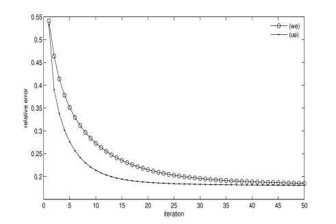
Figure 1. The history of relative error within $50$ iterations.

We next examine $100$ nonlinear system of inequalities with $300$ variables which are produced randomly and each of them is contained by $200$ convex functions. All randomly produced matrices and vectors have entries in $[-10,10].$ First we explain how one of them is made. After generating the matrices $G_{i}\in\mathbb{R}^{300\times 300}$ and the vectors $c_{i}\in\mathbb{R}^{300}$ for $i=1,\cdots,200$, we define the following convex functions

$$f_{i}(x)=x^{T}G_{i}^{T}G_{i}x+c_{i}^{T}x+d_{i}.$$

The vectors $d_{i}$ are calculated such that $f_{i}(y)\leq 0$ where $y=(1,\cdots,1)^{T}.$ Therefore the solution set

$$S=\left\{x|f_{i}(x)\leq 0,~{}~{}i=1,\cdots,200\right\}$$

has at least one point. Similar to the first part of our tests, we assume four strings, i.e. $E=4$, which are contained by $50$ convex functions, i.e., number of elements in each $B_{t}$ is $50$, see Section 4.2. Also in each block we use parallel subgradient projection operator with equal weights and the relaxation parameter $\mu_{t}$ is defined by (4.8).

In addition, the iteration is stopped when $f_{i}^{+}(x)\leq 10^{-4}$ for all $i\in J$ or $\|T(x^{k})-x^{k}\|^{2}\leq 10^{-10}.$ Table 2 explains the mean value of iteration numbers. As it is seen, the iteration number is reduced by (ue).

Table 2. Results of $100$ nonlinear system of inequalities

method	iteration averaging
(ue)	8.49
(we)	30.63

6. Conclusion

In this paper we consider an extrapolated version of string averaging method, which is based on strictly quasi-nonexpansive operators. Our analysis indicates that the generalized relaxation of cutter operators is inherently able to provide more acceleration comparing with results of [15]. As a special case of our algorithm, i.e., Algorithm 1, we consider a wide class of iterative methods for solving linear systems of equations (inequalities) and the subgradient projection method for solving nonlinear convex feasibility problems. Our numerical tests show that using extrapolation strategy we are able to reduce the number of iterations to achieve a feasible point.

Appendix

In this part the classical test problems, used in Section 5, will be explained. For positive integers $i$ and $l$, we use the notations $div(i,l)$ for integer division, i.e., the largest integer not greater than $i/l$, and $mod(i,l)$ for the remainder after integer division, i.e., $mod(i,l)=l(i/l-div(i,l)).$ Here $n$ denotes the number of variables.

1. Extended Powell singular function

   $$g_{i}(x)=x_{j}+10x_{j+1}, mod(i,4)=1$$

   $$g_{i}(x)=\sqrt{5}(x_{j+2}-x_{j+3}), mod(i,4)=2$$

   $$g_{i}(x)=(x_{j+1}-2x_{j+2})^{2}, mod(i,4)=3$$

   $$g_{i}(x)=\sqrt{10}(x_{j}-x_{j+3})^{2}, mod(i,4)=0$$

   $$x^{0}_{l}=3, mod(l,4)=1$$

   $$x^{0}_{l}=-1, mod(l,4)=2$$

   $$x^{0}_{l}=0, mod(l,4)=3$$

   $$x^{0}_{l}=1, mod(l,4)=0$$

   $$n=102 j=2div(i+3,4)-1.$$

2. Chained Wood function

   $$g_{i}(x)=10(x_{j-1}^{2}-x_{j}), mod(i,6)=1$$

   $$g_{i}(x)=x_{j-1}-1, mod(i,6)=2$$

   $$g_{i}(x)=\sqrt{90}(x_{j+1}^{2}-x_{j+2}), mod(i,6)=3$$

   $$g_{i}(x)=x_{j+1}-1, mod(i,6)=4$$

   $$g_{i}(x)=\sqrt{10}(2-x_{j}-x_{j+2}), mod(i,6)=5$$

   $$g_{i}(x)=\frac{1}{\sqrt{10}}(x_{j+2}-x_{j}), mod(i,6)=0$$

   $$x^{0}_{l}=-3, mod(l,2)=1,l\leq 4$$

   $$x^{0}_{l}=-1, mod(l,2)=0,l\leq 4$$

   $$x^{0}_{l}=-2, mod(l,2)=1,l>4$$

   $$x^{0}_{l}=0, mod(l,2)=0,l>4$$

   $$n=68 j=2(div(i,6)+1).$$

3. Extended Rosenbrock function

   $$g_{i}(x)=10(x_{j}^{2}-x_{j+1}), mod(i,2)=1$$

   $$g_{i}(x)=x_{j}-1, mod(i,2)=0$$

   $$x^{0}_{l}=-1.2, mod(l,2)=1$$

   $$x^{0}_{l}=-1, mod(l,2)=0$$

   $$n=101 j=div(i+1,2).$$

4. Broyden tridiagonal function

   $$g_{i}(x)=(3-2x_{j})-x_{j-1}-2x_{j+1}+1$$

   $$x^{0}_{l}=-1, l\geq 1$$

   $$n=200 x_{0}=x_{n+1}=0.$$

5. Penalty function 1

   $$g_{i}(x)=x_{j}-1, 1\leq k\leq 199$$

   $$g_{i}(x)=\frac{1}{\sqrt{1000}}\sum_{i=1}^{n}(x_{j}^{2}-\frac{1}{4}), k=200$$

   $$x^{0}_{l}=l, l\geq 1$$

   $$n=199 x_{0}=x_{n+1}=0.$$

6. Variably dimensioned function

   $$g_{i}(x)=x_{i}-1, 1\leq i\leq n$$

   $$g_{i}(x)=\sum_{j=1}^{n}j(x_{j}-1), i=n+1$$

   $$g_{i}(x)=\left(\sum_{j=1}^{n}j(x_{j}-1)^{2}\right)^{2}, i=n+2$$

   $$x^{0}_{l}=1-\frac{l}{198}, l\geq 1$$

   $$n=198.$$

References

- [1] A. Aleyner and S. Reich, Block-iterative algorithms for solving convex feasibility problems in Hilbert and in Banach spaces, J. Math. Anal. Appl. 343 (2008), 427–435.
- [2] C. Bargetz, V. I. Kolobov, S. Reich and R. Zalas, Linear convergence rates for extrapolated fixed point algorithms, Optimization, 68 (2019), 163–195.
- [3] C. Bargetz, S. Reich and R. Zalas, Convergence properties of dynamic string-averaging projection methods in the presence of perturbations, Numer. Algorithms, 77 (2018), 185–209.
- [4] H.H. Bauschke and J.M. Borwein, On projection algorithms for solving convex feasibility problems, SIAM Rev. 38 (1996), 367–425.
- [5] H.H. Bauschke and P.L. Combettes, A weak-to-strong convergence principle for Fejér-monotone methods in Hilbert spaces, Math. Oper. Res. 26 (2001), 248–264.
- [6] H.H. Bauschke, P.L. Combettes and S.G. Kruk, Extrapolation algorithm for affine-convex feasibility problems, Numer. Algorithms 41 (2006), 239–274.
- [7] H.H. Bauschke, E. Matoušková and S. Reich, Projection and proximal point methods: convergence results and counterexamples, Nonlinear Anal-Theor. 56 (2004), 715–738.
- [8] J.R. Bilbao-Castro, J.M. Carazo, I. García and J.J. Fernandez, Parallel iterative reconstruction methods for structure determination of biological specimens by electron microscopy, International Conference on Image Processing 1 (2003), I–565.
- [9] J.A. Browne, G.T. Herman and D. Odhner, SNARK93: A programming system for image reconstruction from projections, Department of Radiology, University of Pennsylvania, 1993.
- [10] D. Butnariu, R. Davidi, G.T. Herman and I.G. Kazantsev, Stable convergence behavior under summable perturbations of a class of projection methods for convex feasibility and optimization problems, IEEE J-STSP. 1 (2007), 540–547.
- [11] D. Butnariu, S. Reich and A.J. Zaslavski, Stable convergence theorems for infinite products and powers of nonexpansive mappings, Nume. Func. Anal. Opt. 29 (2008), 304–323.
- [12] A. Cegielski, Generalized relaxations of nonexpansive operators and convex feasibility problems, Contemp. Math. 513 (2010), 111–123.
- [13] A. Cegielski, Iterative methods for fixed point problems in Hilbert spaces, Springer, 2013.
- [14] A. Cegielski and Y. Censor, Opial-type theorems and the common fixed point problem, In: Fixed-Point Algorithms for Inverse Problems in Science and Engineering, Springer, 2011.
- [15] A. Cegielski and Y. Censor, Extrapolation and local acceleration of an iterative process for common fixed point problems, J. Math. Anal. Appl. 394 (2012), 809–818.
- [16] A. Cegielski, A. Gibali, S. Reich and R. Zalas, Outer Approximation Methods for Solving Variational Inequalities Defined over the Solution Set of a Split Convex Feasibility Problem, Nume. Func. Anal. Opt. 41 (2020), 1089-1108.
- [17] A. Cegielski, S. Reich, and R. Zalas, Weak, strong and linear convergence of the CQ-method via the regularity of Landweber operators, Optimization 69 (2020), 605–636.
- [18] Y. Censor and T. Elfving, Block-iterative algorithms with diagonally scaled oblique projections for the linear feasibility problem, SIAM J. Matrix Anal. A. 24 (2002), 40–58.
- [19] Y. Censor, T. Elfving and G.T. Herman, Averaging strings of sequential iterations for convex feasibility problems, Studies In Computational Mathematics 8 (2001), 101–113.
- [20] Y. Censor, T. Elfving, G.T. Herman and T. Nikazad, On diagonally relaxed orthogonal projection methods, SIAM J. Sci. Comput. 30 (2008), 473–504.
- [21] Y. Censor, D. Gordon and R. Gordon, BICAV: A block-iterative parallel algorithm for sparse systems with pixel-related weighting, IEEE T. Med. Imaging 20 (2001), 1050–1060.
- [22] Y. Censor and A. Lent, Cyclic subgradient projections, Math. Program. 24 (1982), 233–235.
- [23] Y. Censor and S. Reich, Iterations of paracontractions and firmaly nonexpansive operators with applications to feasibility and optimization, Optimization 37 1996, 323–339.
- [24] Y. Censor and A. Segal, On the string averaging method for sparse common fixed-point problems, Int. T. Oper. Res. 16 (2009), 481–494.
- [25] Y. Censor and E. Tom, Convergence of string-averaging projection schemes for inconsistent convex feasibility problems, Optim. Method. Softw. 18 (2003), 543–554.
- [26] Y. Censor and A.J. Zaslavski, Convergence and perturbation resilience of dynamic string-averaging projection methods, Comput. Optim. Appl. 54 (2013), 65–76.
- [27] Y. Censor and A.J. Zaslavski, String-averaging projected subgradient methods for constrained minimization, Optim. Method. Softw. 29 (2014), 658–670.
- [28] Y. Censor and A.J. Zaslavski, Strict Fejér monotonicity by superiorization of feasibility-seeking projection methods, J. Optimiz. Theory App. 65 (2015), 172–187.
- [29] P.L. Combettes, in Quasi-Fejérian Analysis of Some Optimization Algorithm, Studies In Computational Mathematics 8 (2001), 115–152.
- [30] P.L. Combettes and I. Yamada, Compositions and convex combinations of averaged nonexpansive operators, J. Math. Anal. Appl. 425 (2015), 55–70.
- [31] G. Crombez, Finding common fixed points of strict paracontractions by averaging strings of sequential iterations, J. Nonlinear Convex A. 3 (2002), 345–351.
- [32] G. Crombez, Finding common fixed points of a class of paracontractions, ACTA Math. Sci. 103 (2004), 233–241.
- [33] R. Davidi, Algorithms for Superiorization and Their Applications to Image Reconstruction, PhD thesis, City University of New York, USA, 2010.
- [34] R. Davidi, G.T. Herman and Y. Censor, Perturbation-resilient block-iterative projection methods with application to image reconstruction from projections, Int. T. Oper. Res. 16 (2009), 505–524.
- [35] L.T. Dos Santos, A parallel subgradient projections method for the convex feasibility problem, J. Comput. Appl. Math. 18 (1987), 307–320.
- [36] P.B.B. Eggermont, G.T. Herman and A. Lent, Iterative algorithms for large partitioned linear systems, with applications to image reconstruction, Linear Algebra Appl. 40 (1981), 37–67.
- [37] T. Elfving, Block-iterative methods for consistent and inconsistent linear equations, Numer. Math. 35 (1980), 1–12.
- [38] T. Elfving and T. Nikazad, Properties of a class of block-iterative methods, Inverse Probl. 25 (2009), 115011.
- [39] L. Elsner, I. Koltracht and M. Neumann, Convergence of sequential and asynchronous nonlinear paracontractions, Numer. Math. 62 (1992), 305–319.
- [40] D. Gordon and R. Gordon, Component-averaged row projections: A robust, block-parallel scheme for sparse linear systems, SIAM J. Sci. Comput. 27 (2005), 1092–1117.
- [41] E.S. Helou, Y. Censor, T.B. Chen, I.L. Chern, A.R. De Pierro, M. Jiang and H. H.S. Lu, String-averaging expectation-maximization for maximum likelihood estimation in emission tomography, Inverse Probl. 30 (2014), 055003.
- [42] G.T. Herman, Fundamentals of computerized tomography: image reconstruction from projections, Springer, London, 2009.
- [43] M. Jiang and G. Wang, Convergence studies on iterative algorithms for image reconstruction, IEEE T. Med. Imaging 22 (2003), 569–579.
- [44] L. Lukšan and J. Vlcek, Test problems for unconstrained optimization, Academy of Sciences of the Czech Republic, Institute of Computer Science, Technical Report, 897 (2003).
- [45] T. Nikazad and M. Abbasi, Perturbation-Resilient Iterative Methods with an Infinite Pool of Mappings, SIAM J. Numer. Anal. 53 (2015), 390–404.
- [46] T. Nikazad, M. Abbasi and T. Elfving, Error minimizing relaxation strategies in Landweber and Kaczmarz type iterations, J. Inverse Ill-pose. P. 25 (2017) 35–56.
- [47] T. Nikazad, M. Abbasi and M. Mirzapour, Convergence of string-averaging method for a class of operators, Optim. Method. Softw. 31 (2016), 1189–1208.
- [48] T. Nikazad, R. Davidi and G.T. Herman, Accelerated perturbation-resilient block-iterative projection methods with application to image reconstruction, Inverse Probl. 28 (2012), 035005.
- [49] T. Nikazad and M. Mirzapour, Generalized relaxation of string averaging operators based on strictly relaxed cutter operators, J. Nonlinear Convex A. 18 (2017), 431–450.
- [50] S. Penfold, R.W. Schulte, Y. Censor, V. Bashkirov, S. McAllister, K. Schubert and A.B. Rosenfeld, Block-iterative and string-averaging projection algorithms in proton computed tomography image reconstruction. In Y. Censor, M. Jiang, & G. Wang (Eds.), Biomedical mathematics: Promising directions in imaging, therapy planning and inverse problems (pp. 347–367), Medical Physics Publishing, Wisconsin, USA, 2010.
- [51] S. Reich and R. Zalas, A modular string averaging procedure for solving the common fixed point problem for quasi-nonexpansive mappings in Hilbert space, Numer. Algorithms 72, (2016), 297–323.
- [52] H.J. Rhee, An application of the string averaging method to one-sided best simultaneous approximation, J. Korean Soc. Math. Educ. Ser. B: Pure Appl. Math. 10 (2003), 49–56.