Joint Linear Trend Recovery Using $\ell_{1}$ Regularization

Keywords: Change Point, Estimation consistency, $\ell_{1}$ regularization, Linear trend filtering, Sign consistency.

1 Introduction

For a naturally-occurring time series with observation $y_{t}$ and underlying mean $\mu_{t}^{0}$ at $1\leq t\leq n$, an important issue is to recover the trend of the underlying mean vector, ${\boldsymbol{\mu}}^{0}=(\mu^{0}_{1},\cdots,\mu^{0}_{n})^{\prime}$. Here ${\boldsymbol{\mu}}^{0}$ often exhibits various kinds of trends in many real applications. For example, in the analysis of DNA sequences, ${\boldsymbol{\mu}}^{0}$ is assumed to be piece-wise constant (Braun and Muller, 1998; Huang et. al, 2005). However, in financial time series, ${\boldsymbol{\mu}}^{0}$ is often assumed to be piece-wise linear (Taylor, 2008). Other applications can also be found in macroeconomics (Hodrick and E. Prescott, 1997), climate research (Baillie and Chung, 2002) and social sciences (Levitt, 2004). Various trend filtering methods have been developed to recover the underlying mean vector from noisy data. We refer Kim et al. (2009) for a complete review of many different trend filtering methods and applications.

1.1 Model assumptions and some background

Consider a model

$${\rm(I)}\quad y_{t} =\mu^{0}_{t}+\varepsilon_{t},~{}1\leq t\leq n,$$ (1)

where $\varepsilon_{t}$ is the random noise with mean $0$ and variance $\sigma^{2}$, $1\leq t\leq n$. The interest is to recover the mean vector with joint piece-wise linear trend, meaning the underlying mean vector in model (1) satisfying:

$${\rm(I\!I)}\quad\mu_{t}^{0} =a_{j}+b_{j}t,~{}t_{j-1}\leq t\leq t_{j}-1,~{}j=1,\cdots,J+1,~{}1\leq t\leq n,$$ (2)

and

$${\rm(I\!I\!I)}\quad a_{j-1}+b_{j-1}t_{j}=a_{j}+b_{j}t_{j},~{}1\leq j\leq J.$$ (3)

Here $t_{0}=1$ and $t_{J+1}=n+1$. For $1\leq j\leq J$, $t_{j}\in\{1,\cdots,n\}$ denote change points or kink points where consistent linear trend changes. The $(a_{j},b_{j}),j=1,\cdots,J+1$ are $J+1$ pairs of local intercepts and slopes. Model assumption (I​I​I) requires that true means at the kink point to be fitted consistently from two corresponding adjacent linear trends. See a toy example in Figure 1 (a). To recover the mean vector ${\boldsymbol{\mu}}^{0}$ under model I–I​I​I, one can always get a maximum likelihood or least squares estimation of those $(a_{j},b_{j})$’s first by controlling the number of the kink points. To list a few, one can see for example Feder (1975a,b), Bai and Perron (1998) and Bhattacharya (1994).

However, such an dynamic optimization approach is computational expensive (Hawkins, 2001). Since the introduction of the well-known least absolute shrinkage estimator (LASSO) in Tibshirani (1996), the $\ell_{1}$ regularization technique has been widely used in many problems when the underlying model or the true coefficients vector has some sparse properties. Here sparsity mean the true model containing many zeros coefficients, but only a few non-zero ones. The change point detection problem can be treated as a typical high-dimensional sparse model in terms of two properties: the dimension is high since the number of unknown means equals $n$, the model is sparse since there are and only a few true change points. Thus an $\ell_{1}$ regularization approach can be applied to detect non-zero changes, and therefore identify the change points. For example, when the mean vector in (1) is piece-wise constant, the jump (adjacent difference mean) vector consists of most zeros except only a few non-zeros where abrupt changes occur. One can penalize the $\ell_{1}$ norm of the jump vector to obtain a piece-wise constant mean estimation,

$$\widehat{\boldsymbol{\mu}}_{\rm TV}(\lambda_{n})=\mathop{\rm arg\,min}\{(1/2)\sum_{t=1}^{n}(y_{t}-\mu_{t})^{2}+\lambda_{n}\sum_{t=2}^{n}|\mu_{t}-\mu_{t-1}|\},$$ (4)

where $\lambda_{n}\sum_{t=2}^{n}|\mu_{t}-\mu_{t-1}|$ for some positive $\lambda_{n}$ is a total variation (TV) penalty. Both theoretical and computational properties of $\widehat{\boldsymbol{\mu}}_{\rm TV}(\lambda_{n})$ in (4) have been well studied by Harchaoui and Lévy-Leduc (2010) and Rinaldo (2009).

Model in (4) was used to detect abrupt change points where all $b_{j}$’s are $0$ in linear model (1). A similar idea can be adopted for the recovery of joint piece-wise linear trend. For $3\leq t\leq n$, we denote $\beta_{t}=\mu_{t}+\mu_{t-2}-2\mu_{t-1}$ as the potential slope changes at $t-1$ and ${\boldsymbol{\beta}}=(\beta_{1},\cdots,\beta_{n})^{\prime}$. Since there are only a few local slopes for the underlying slope change vector, ${\boldsymbol{\beta}}^{0}$ exhibits some sparse property. Thus, instead of controlling the number of non-zero slope changes directly, one can obtain a piece-wise linear mean trend estimation for model I–I​I​I  by penalizing the $\ell_{1}$ norm of the slope change vector,

$$\widehat{\boldsymbol{\mu}}(\lambda_{n})=\mathop{\rm arg\,min}\left\{(1/2)\sum_{t=1}^{n}(y_{t}-\mu_{t})^{2}+\lambda_{n}\sum_{t=3}^{n}|\mu_{t}+\mu_{t-2}-2\mu_{t-1}|\right\},$$ (5)

where $\lambda_{n}>0$ is a tuning parameter controlling the number of estimated linear pieces. Larger $\lambda_{n}$ will generate smaller number of joint linear pieces. Model (5) is the $\ell_{1}$ linear filtering method studied in Kim et al. (2009), as a comparison with the Hodrick-Prescott (H-P) filtering (Hodrick and Prescott, 1997), a trend filtering approach to recover the piece-wise quadratic curve. Kim et al. (2009) discussed some basic properties of $\widehat{\boldsymbol{\mu}}(\lambda_{n})$:

• (P1): As $\lambda_{n}\to 0$, then $\widehat{\boldsymbol{\mu}}(\lambda_{n})$ converges to ${\mathbf{y}}=(y_{1},\cdots,y_{n})^{\prime}$.

• (P2): As $\lambda_{n}\to\infty$, $\widehat{\boldsymbol{\mu}}(\lambda_{n})$ converges to the best affine fit to ${\mathbf{y}}$.

Tibshirani and Taylor (2011) also provided some interesting dual algorithms to solve solution paths of a linear trend filter (LTF) in (5).

However, many important questions on the properties of an LTF have not been answered. Will an LTF (5) find all kink points asymptotically? If all kink points are detected, will the joint piece-wise linear mean trend be recovered consistently? How to choose an optimal $\lambda$ to obtain a well-behaved LTF? In this paper, we will investigate some asymptotic properties of an LTF under some sufficient conditions. Specifically, under the joint piece-wise linearity assumption in model I–I​I​I, we will first investigate some rate estimation consistency of an LTF if a tuning parameter is well chosen. Then, we will provide some sufficient conditions under which all underlying multiple kink points can be detected correctly in a large probability. More importantly, those slope changes in direction can be recovered consistently for a well chosen $\lambda$. As a by-product, we will justify that a weak irrepresentable condition is not needed for the consistent change point detection.

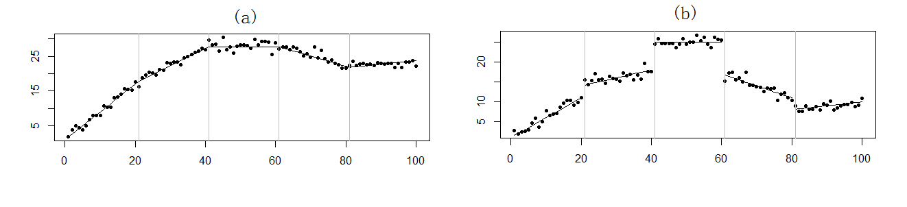
Figure 1: Linear Trend toy example. Dots represent observations at some locations. The underlying mean trend are connected by solid lines. (a): piece-wise linear trend is jointed; (b): piece-wise linear trend is not jointed

1.2 Notations and Preliminaries

We list some preliminaries and notations to end this section. Suppose there are $J+1$ linear segments, separated by kink points $t_{j}$’s for $1\leq j\leq J$. We make the following notations:

• ${\cal J}=\{t_{j},1\leq j\leq J\}$, the collection of the kink points;

• ${\cal B}_{j}=\{t_{j-1},\cdots,t_{j}-1\}$, the subset of $j$th segment;

• $|{\cal B}_{j}|$, the cardinal value of ${\cal B}_{j}$;

• Suppose $b_{1},\cdots,b_{J},b_{J+1}$ are all local slopes. Then the sub-differentials

  $$c_{j}=\partial\sum_{k=2}^{J+1}|b_{k}-b_{k-1}|/\partial b_{j}=\left\{\begin{array}[]{ll}\mbox{sgn}(b_{j}-b_{j-1})-\mbox{sgn}(b_{j+1}-b_{j})&\quad{\rm for}~{}3\leq j\leq J\\ \mbox{sgn}(b_{J-1}-b_{J-2})&\quad{\rm for}~{}j=J+1\\ -\mbox{sgn}(b_{2}-b_{1})&\quad{\rm for}~{}j=2\end{array}\right.,$$ (9)

  where $\mbox{sgn}(x)=1,s,-1$ if $x>0,=0,<0$ with $-1<s<1$;

• Correspondingly, ${{\cal J}^{0}}=\{t^{0}_{j},1\leq j\leq J^{0}\}$, the true kink point set; $b_{j}^{0},1\leq j\leq J^{0}+1$ are the underlying local slopes ${\cal B}_{j}^{0}=\{t_{j-1}^{0},\cdots,t_{j}^{0}-1\}$ is the true $j$th segment and $|{\cal B}_{j}^{0}|$ is its cardinal value;

• $b_{\min}^{0}=\min_{1\leq j\leq J^{0}}|{\cal B}_{j}^{0}|$, the smallest segment size among all linear pieces;

• $a_{n}=\min_{1\leq j\leq J^{0}}|\mu_{t_{j}+1}^{0}+\mu_{t_{j}-1}^{0}-2\mu_{t_{j}}^{0}|=\min_{1\leq j\leq J^{0}}|b_{j+1}^{0}-b_{j}^{0}|$ for $j\in{\cal J}^{0}$, the smallest slope change at true kink points.

If $\widehat{\boldsymbol{\mu}}(\lambda_{n})$ is an LTF for $\lambda_{n}>0$, then $\widehat{t}_{j+1}(\lambda_{n})$, $\widehat{\cal J}(\lambda_{n})$, $\widehat{\cal B}_{j}$ are defined correspondingly. We sometimes omit $\lambda_{n}$ from the estimation without causing any confusion.

1.3 Structure of the paper

The rest of the paper is presented as follows. In Section 2, we give two different transformations of the $\ell_{1}$ linear trend filtering model and discuss some corresponding computational and analytical properties of two types of LTF solutions. We present our main asymptotic results in Section 3. In this section, we provide some sufficient conditions under which an LTF can have some rate estimation consistency and detect those kink points consistently. The effect of weak irrepresentable condition on change point detection is also discussed in this section. In Section 4, we provide some numerical studies containing both simulation studies. We summarize the paper with some discussions in Section 5. Finally, we give all technical proofs in the Appendix.

2 Analytical properties of $\ell_{1}$ trend filter

Let the jump value, $\nu_{t}\equiv\mu_{t}-\mu_{t-1}$ be the slope between $t-1$ and $t$ for $2\leq t\leq n$. Then the slope change $\beta_{t}=\mu_{t}+\mu_{t-2}-2\mu_{t-1}=\nu_{t}-\nu_{t-1}$, for $3\leq t\leq n$. To unify the notation, we also let $\nu_{1}=\mu_{1}$, $\beta_{1}=\mu_{1}$, and $\beta_{2}=\mu_{2}-\mu_{1}$. Below we give two different expressions of the linear trend filtering model in (5).

2.1 Total variation transformation

Under model assumptions I–I​I​I, the underlying slope vector ${\boldsymbol{\nu}}^{0}=(\nu_{1}^{0},\cdots,\nu_{n}^{0})^{\prime}$ is piece-wise constant with only a few abrupt changes. Thus, we can rewrite model (5) into a penalized regression model of slope vector ${\boldsymbol{\nu}}=(\nu_{1},\cdots,\nu_{n})^{\prime}$ with the total variation penalty,

$$\begin{array}[]{ll}\widehat{\boldsymbol{\nu}}(\lambda_{n})&=\mathop{\rm arg\,min}f({\boldsymbol{\nu}},\lambda_{n})\\ &=\mathop{\rm arg\,min}\left\{(1/2)\sum_{t=1}^{n}(y_{t}-\sum_{j=1}^{n}x_{tj}\nu_{j})^{2}+\lambda_{n}\sum_{t=3}^{n}|\nu_{t}-\nu_{t-1}|\right\},\end{array}$$ (12)

where $x_{tj}=1$ for $1\leq j\leq t$ and $0$ otherwise for $1\leq t\leq n$. Thus, by modifying the pathwise decent algorithm in Friedman et al. (2007), we can find an estimation of the slope vector $\widehat{\boldsymbol{\nu}}$ first, and then use the cumulative sum to obtain an estimation of $\widehat{\boldsymbol{\mu}}$. Below we give a detailed description of the modified pathwise decent algorithm.
Modified Pathwise Decent Algorithm

• 1. Start from $\lambda=0$.

• 2. Increase $\lambda$ with a reasonable small value and run the following decent step and fusion step, until no further changes occur.

• 3. Repeat 2 until a target $\lambda$ is reached.

Suppose $\widetilde{\boldsymbol{\nu}}$ is the slope vector obtained from the last step. Then the current step includes both decent cycle and fusion cycle as follows.

• Decent cycle: In (12), check $\partial f/\partial\nu_{k}=0$ for $\nu_{k}$ belonging to the following three intervals:

  $$(-\infty,\min\{\widetilde{\nu}_{k-1},\widetilde{\nu}_{k+1}\}],~{}(\min\{\widetilde{\nu}_{k-1},\widetilde{\nu}_{k+1}\},\max\{\widetilde{\nu}_{k-1},\widetilde{\nu}_{k+1}\}],~{}(\max\{\widetilde{\nu}_{k-1},\widetilde{\nu}_{k+1}\},\infty),$$

  where $\widetilde{\nu}_{k-1}$ and $\widetilde{\nu}_{k+1}$ are solutions from the last step. If no solution is found, update $\nu_{k}$ into the one between $\widetilde{\nu}_{k-1}$ and $\widetilde{\nu}_{k+1}$ such that $f$ decreases more. Specifically, we solve

  $$\nu_{k}=(n-k+1)^{-1}\left(\sum_{i=k}^{n}y_{i}-\sum_{i=1}^{n}a_{ik}\widetilde{\nu}_{i}+\lambda\cdot g\right),$$ (13)

  where $a_{ik}=n-k+1,0$ and $n-i+1$ for $i<k$, $i=k$ and $i>k$, where $g=0,\pm 1$ and $\pm 2$ for $k=1$, $2$ and $3$ for $3\leq k\leq n-1$. Here “$+$” or “$-$” is decided in terms of which interval the $\nu_{k}$ is checked. For example, if $\widetilde{\nu}_{k-1}<\widetilde{\nu}_{k+1}$ for some $3\leq k\leq n-1$, then $g=2$ and $-2$ for $\nu_{k}<\widetilde{\nu}_{k-1}$ and $\nu_{k}>\widetilde{\nu}_{k+1}$, respectively.

• Fusion cycle: Enforcing $\nu_{k}=\nu_{k-1}=\cdots=\nu_{k-m}$ for $1\leq m\leq k-1$ and assuming $\nu_{k}=\cdots=\nu_{k-m}=\alpha$ in the penalized objective function $f$, check $\partial f/\partial\alpha=0$ for $\alpha$ belongs to any of the following three intervals:

  $$(-\infty,\min\{\widetilde{\nu}_{k-m},\widetilde{\nu}_{k+1}\}],~{}(\min\{\widetilde{\nu}_{k-m},\widetilde{\nu}_{k+1}\},\max\{\widetilde{\nu}_{k-m},\widetilde{\nu}_{k+1}\}],~{}(\max\{\widetilde{\nu}_{k-m},\widetilde{\nu}_{k+1}\},\infty).$$ (14)

  If a solution $\alpha$ can be found, then we accept the fusion setting. To be more specific, we $\alpha$ is

  $$\left(\sum_{i=k-m}^{n}y_{i}d_{m+i+1-k}-\sum_{i=1}^{m+n+1-k}d_{i}\sum_{i=1}^{k-m+1}\widetilde{\nu}_{i}-\sum_{i=k+1}^{n}(\widetilde{\nu}_{i}\sum_{j=m+1}^{m+1+n-i}d_{j})+\lambda g\right)\left/\sum_{i=1}^{m+n-k+1}d_{i}^{2}\right.,$$ (15)

  for three intervals in (14), where $d_{i}=i$ and $m+1$ for $1\leq i\leq m$ and $i\leq m+1$, and $g$ is defined in the decent step.

Here (13) and (15) can be derived by direct computation.

2.2 LASSO transformation

Another possible approach to obtain $\widehat{\boldsymbol{\mu}}(\lambda_{n})$ is to consider model (5) as a LASSO model of the slope change vector ${\boldsymbol{\beta}}=(\beta_{1},\cdots,\beta_{n})^{\prime}$,

$$\widehat{\boldsymbol{\beta}}(\lambda)=\mathop{\rm arg\,min}\left\{(1/2)\sum_{t=1}^{n}(y_{t}-\sum_{j=1}^{n}z_{tj}\beta_{j})^{2}+\lambda_{n}\sum_{j=3}^{n}|\beta_{j}|\right\},$$ (16)

where $z_{t1}=1$ for $1\leq t\leq n$, $z_{tj}=t-j+1$ for $j\leq t$ and $z_{tj}=0$ for $j>t$. Thus the existing algorithm for LASSO can be adopted to solve ${\boldsymbol{\beta}}=(\beta_{1},\cdots,\beta_{n})^{\prime}$ in (16) first. A mean estimation can be obtained by $\widehat{\boldsymbol{\mu}}(\lambda)={\mathbf{Z}}\widehat{\boldsymbol{\beta}}(\lambda)$, where ${\mathbf{Z}}$ is matrix consisting of all $z_{tj}$’s. Theoretically, for a given tuning parameter $\lambda$, both (12) and (16) should provide the same solution. However, since the tuning parameter selection technique is involved, those two approaches can provide different final trend filters. Combining with some existing tuning parameter selection techniques, LASSO model (16) turns to generate more non-zero $\widehat{\beta}_{j}$’s with small values around the true kink points than the pathwise algorithm does. In practice, the pathwise algorithm is preferred if one is more interested recovering those change points. However, LASSO model is preferred is one cares more about the mean trend estimation. In section 4.2, we use some simulation studies to demonstrate those differences in more details. We also provide a theoretical justification in Section 3.2.

In the next section, we investigate some asymptotic properties of an LTF, $\widehat{\boldsymbol{\mu}}(\lambda_{n})$ in (5). We provide some sufficient conditions under which a well-behaved $\widehat{\boldsymbol{\mu}}(\lambda_{n})$ can be reached.

3 Asymptotic properties

In this section, we study the asymptotic properties of an LTF $\widehat{\boldsymbol{\mu}}_{n}$. In some cases, we aim to find an almost “unbiased” estimator of the mean trend vector, which motivate us to obtain some rate estimation consistency properties under some conditions in Section 3.1. In other cases, we are more interested in the recovery of kink points, which motivate us to investigate some sufficient conditions under which those underlying kink points can be identified consistently.

We first make the following assumption on the random noise.

(A1). Random noise $\varepsilon_{i}$’s are i.i.d. with mean $0$ and finite variance $\sigma^{2}$. Furthermore, they are sub-Gaussian in the sense that $E[\exp(t\varepsilon_{i})]\leq\exp(\sigma^{2}t^{2}/2),1\leq i\leq n.$

3.1 Estimation consistency properties

Consider a multiple change point model in I–I​I​I. In order to obtain an almost “unbiased” estimator of the unknown mean vector ${\boldsymbol{\mu}}^{0}$ from model (5), we make the following additional assumption on the underlying ${\boldsymbol{\mu}}^{0}$.

(A2). The underlying mean ${\boldsymbol{\mu}}^{0}$ in model (1) has at most $J_{\max}$ local linear pieces.

From (P2) in Section 2, it is always reasonable to generate an LTF $\widehat{\boldsymbol{\mu}}(\lambda_{n})$ with finite number of linear pieces.

Lemma 1

There exists $\lambda_{0}>0$ such that $\widehat{\boldsymbol{\mu}}(\lambda_{n})$ always has at most $J_{\max}$ local linear pieces for any $\lambda>\lambda_{0}$.

The proof of Lemma 1 is skipped since it is a direct result of (P2) in Section 1. Then we have the following rate consistency of the mean estimation.

Theorem 1

Suppose (A1) and (A2) hold for model I–I​I​I. Let

$$\lambda_{n}=16^{-1}\sigma A(BJ_{\max}\log n)^{1/2}n^{-1/2}-32^{-1/2}\sigma(J_{\max})^{1/2}n^{-1/2}$$

for some $0<A<1$ and $B>2(1-A)^{-2}$. Suppose $\lambda_{n}>\lambda_{0}$ for the $\lambda_{0}$ in Lemma 1. Then for an LTF $\widehat{\boldsymbol{\mu}}(\lambda_{n})$ in (5),

$$P\left(n^{-1/2}\|\widehat{\boldsymbol{\mu}}-{\boldsymbol{\mu}}^{0}\|_{2}\geq\sigma(BJ_{\max}\log n/n)^{1/2}\right)\leq J_{\max}n^{[1-B(1-A)^{2}/2]J_{\max}}.$$

Theorem 1 reveals that we can obtain a consistent estimator of the underlying mean vector ${\boldsymbol{\mu}}^{0}$ by choosing $\lambda_{n}$ appropriately. In addition, the consistency rate is $O(\log(n)/n)^{1/2})$, which is same as the one obtained by Harchaoui and Lévy-Leduc (2010) for the piece-wise constant model in model (4). Such a consistency rate, $O(\log n/n)^{1/2}$, is also comparable with the optimal rate obtained by Yao and Au (1988), $O(n^{-1/2})$. In their work, the least squares estimation method is used to recover the piece-wise constant when the number of change-points is bounded. We postpone the detailed proof to the Appendix.

3.2 Sign consistency properties

In the last section, we provide some rate estimation consistency of the mean estimator $\widehat{\boldsymbol{\mu}}(\lambda_{n})$ if the number of kink points for both $\widehat{\boldsymbol{\mu}}(\lambda_{n})$ and $\widehat{\boldsymbol{\mu}}^{0}$ are bounded. In many real applications, we are more interested in the detection of underlying kink points where the underlying linear trends change. In this section, we investigate the consistency of the kink points detection. More specifically, we provide some sufficient conditions under which not only the locations but also the directions of those slope changes are recovered with a large probability. We make the following assumptions on the underlying model and the tuning parameter $\lambda_{n}$:

(B1). $\lambda_{n}\leq 2a_{n}b_{\min}^{0}$;

(B2). $a_{n}^{2}(b_{\min}^{0})^{3}\to\infty$;

(B3). (a) $(\lambda_{n})^{1/2}\to\infty$; (b) $(2+\log((n-J^{0}))/\lambda_{n}<28\delta/\sigma$ for some constant $0<\delta<1$.

Here (B2) requires either $a_{n}$, the smallest slope changes between any two adjacent linear segments, or $b_{\min}^{0}$, the smallest linear segment size to be large enough. Assumptions in (B3) require the tuning parameter $\lambda_{n}$ to grow with $n$. In addition, (B3-b) also provides a lower bound of the growth rate. (B1) provides some further information on the growth speeds among $\lambda_{n}$, $a_{n}$ and $b_{\min}^{0}$. Notice that there is some redundancy among those conditions. For example, one can also deduce (B2) from (B1) and (B3-a). Here we list all those conditions for a better understanding of the growth rates of $a_{n}$, $b_{\min}^{0}$ and $\lambda_{n}$.

Denote an event for identifying all kink points correctly as,

$${\cal S}^{1n}(\lambda_{n})=\{\widehat{\cal J}(\lambda_{n})={\cal J}^{0}\}.$$

Furthermore, a stronger event for detecting directions of slope changes correctly is,

$${\cal S}^{n}(\lambda_{n})=\left\{{\cal S}^{1n}(\lambda_{n})\bigcap\{\mbox{sgn}(\widehat{\mu}_{i+1}(\lambda_{n})+\widehat{\mu}_{i-1}(\lambda_{n})-2\widehat{\mu}_{i}(\lambda_{n}))=\mbox{sgn}(\mu^{0}_{i+1}+\mu^{0}_{i-1}-2\mu^{0}_{i}),\forall i\in{\cal J}^{0}\}\right\}.$$

Here ${\cal S}^{n}(\lambda_{n})$ is stronger than ${\cal S}^{1n}(\lambda_{n})$ since not only locations of all kink points (where $\mu^{0}_{i+1}+\mu^{0}_{i-1}-2\mu^{0}_{i}\neq 0$) are detected, but also directions of slope changes (sign of $\mu^{0}_{i+1}+\mu^{0}_{i-1}-2\mu^{0}_{i}$) at those locations are correctly recovered. We call a kink point having a positive (negative) sign when slope increases (decreases) at this location. Analogous to the variable selection, we give the following two definitions on the selection consistency and sign consistency of kink points.

Definition 1

$\widehat{\boldsymbol{\mu}}$ is kink point detection consistent if $P({\cal S}^{1n}(\lambda_{n}))\to 1$ when $n\to\infty$.

Definition 2

$\widehat{\boldsymbol{\mu}}$ is kink point sign consistent if $P({\cal S}^{n}(\lambda_{n}))\to 1$ when $n\to\infty$.

In general, it is much more complicated to check the event ${\cal S}^{1n}$ directly. So we investigate the kink point sign consistency in Definition 2 instead of the kink point detection consistency in Definition 1. In the following theorem, we provide some sufficient conditions under which an LTF $\widehat{\boldsymbol{\mu}}(\lambda_{n})$ is kink point sign consistent.

Theorem 2

Suppose (A1) and (B1-B3) hold for a time series model I–I​I​I. Then for an $\ell_{1}$ trend filter $\widehat{\boldsymbol{\mu}}(\lambda_{n})$ in (5), we have

$$\lim_{n\to\infty}P({\cal S}^{n}(\lambda_{n}))=1.$$

The proof of Theorem 2 is given in the Appendix. Theorem 2 indicates that model (5) can recover all kink points of a joint piece-wise linear mean trend. Furthermore, the LTF based on a well chosen $\lambda_{n}$ can catch all directions of slope changes at those kink points with a large probability. This result is the extension of the study in Rinaldo (2009), where change point locations are recovered for the piece-wise constant trend using the total variation penalty.

3.3 Additional comments

We make two additional comments regarding the above asymptotic results in Section 3.1 and 3.2.

Comment 1: Weak irrpresentable condition is not necessary for kink point sign consistency.

In Section 2.2, we discussed that the $\ell_{1}$ trend filtering model can be also written into a LASSO model in (16) with the low triangular design matrix ${\mathbf{Z}}$. Theorem 2 of Zhao and Yu (2006) states that that the weak irrepresentable condition is a necessary condition for a LASSO solution to be sign consistent under two regularity conditions. Consider a general LASSO model,

$$\widehat{\boldsymbol{\beta}}^{(g)}(\lambda)=\mathop{\rm arg\,min}\left\{(1/2)\sum_{i=1}^{n}(y_{i}^{(g)}-\sum_{j=1}^{p}x^{(g)}_{ij}\beta^{(g)}_{j})^{2}+\lambda\sum_{j=1}^{p}|\beta_{j}^{(g)}|\right\},$$ (17)

where $(y_{i}^{(g)},x^{(g)}_{i1},\cdots,x^{(g)}_{ip})$ and $(\beta_{1}^{(g)},\cdots,\beta_{p}^{(g)})^{\prime}$ represent the observed data and coefficients vector in the general regression model. Let ${\mathbf{X}}^{(g)}=({\mathbf{X}}^{(g)}_{{\mathbf{1}}},{\mathbf{X}}^{(g)}_{{\mathbf{2}}})$ be the covariate matrix, where ${\mathbf{X}}^{(g)}_{{\mathbf{1}}}$ and ${\mathbf{X}}^{(g)}_{{\mathbf{2}}}$ include only the important and unimportant covariates, respectively. Let ${\mathbf{s}}^{(g)}_{{\mathbf{1}}}=\mbox{sgn}({\boldsymbol{\beta}}_{{\mathbf{1}}})$ consist of sign mappings of non-zero coefficients in the true model. Then model (17) satisfies the weak irrepresentable condition if

$$|{\mathbf{X}}^{(g)^{\prime}}_{{\mathbf{2}}}{\mathbf{X}}^{(g)}_{{\mathbf{1}}}({\mathbf{X}}^{(g)^{\prime}}_{{\mathbf{1}}}{\mathbf{X}}^{(g)}_{{\mathbf{1}}})^{-1}{\mathbf{s}}^{(g)}_{{\mathbf{1}}}|<{\mathbf{1}}.$$ (18)

Lemma 2

(Zhao and Yu, 2006) Supose two regularity conditions are satisfied for the designed matrix ${\mathbf{X}}^{(g)}$: (1) there exists a positive definite matrix $C$ such that the covariance matrix $({\mathbf{X}}^{(g)})^{\prime}{\mathbf{X}}^{(g)}/n\to C$ as $n\to\infty$, and (2) $\max_{1\leq i\leq n}({\mathbf{x}}_{i}^{(g)})^{\prime}{\mathbf{x}}_{i}^{(g)})/n\to 0$ as $n\to\infty.$ Then LASSO is general sign consistent only if there exists $N$ so that the weak irrepresentable condition in (18) holds for $n>N$.

Unfortunately, the LASSO model in (16) does not satisfies the weak irrepresentable condition (See an counter example in the Appendix). However, there is no contradiction between the sign consistency result in Theorem 2 and Lemma 2 since those two regularity conditions in Theorem 2 in Lemma 2 are not satisfied for the design matrix ${\mathbf{Z}}$ in (16) because of the following lemma.

Lemma 3

The design matrix ${\mathbf{Z}}$ in model (16) has two properties: (a) $\rho_{1}<1/(4n)\to 0$ when $n\to\infty$, where $\rho_{1}$ is the smallest eigenvalue of ${\mathbf{Z}}^{\prime}{\mathbf{Z}}/n$ and (b) $\max_{1\leq i\leq n}{\mathbf{z}}_{i}^{\prime}{\mathbf{z}}_{i}/n\geq n^{2}/4$.

Lemma 3 can be verified easily and we skip the detailed proof in this manuscript. Two properties (a) and (b) in Lemma 3 means the both regularity conditions (1) and (2) in Lemma 2 are violated. Thus Theorem 2 is not against Lemma 2. In other words, Theorem 2 indicates that the weak irrepresentable condition is not necessary for the change point detection.

Comment 2: An LTF may not reach the estimation consistency and sign consistency simultaneously.

The rate estimation consistency in Theorem 1 holds for $\lambda_{n}=O(\log(n)/n)$. However, from (B3-b), we know one of the sufficient conditions for the sign consistency in Theorem 2 requiring $\lambda_{n}>O(\log(n))$. So an $\ell_{1}$ trend filter may not be able to reach the estimation consistency and sign consistency simultaneously. However, this claim is not theoretically justified since all conditions assumed in both Theorem 1 and 2 are sufficient.

4 Numerical studies

In this section, we use some simulation studies to demonstrate the performance of the $\ell_{1}$ trend filter.

4.1 Tuning parameter selection

As stated in Section 2, for every $\lambda>0$, we can first find an optimizer $\widehat{\boldsymbol{\nu}}(\lambda)$ of (12) using the modified pathwise decent algorithm. For such a $\lambda>0$, an $\ell_{1}$ trend filter is obtained from corresponding cummalative summation. Since $\lambda$ controls the number of abrupt changes in $\widehat{\boldsymbol{\nu}}(\lambda)$, it is important to choose an optimal tuning parameter, $\lambda_{\rm opt}$, from a sequence of $\lambda\in(\lambda_{\min},\lambda_{\max})$, where $\lambda_{\max}$ is a sufficient large $\lambda$ such that $\widehat{\boldsymbol{\mu}}(\lambda_{n})$ reaches the best affine fit to ${\mathbf{y}}$. For a fixed $\lambda>0$, model (12) is a modeling procedure including both model selection and model fitting. Zou et al. (2007) justified the number of non-zero estimates of a LASSO estimates is an unbiased estimates of the degrees of the freedom of the LASSO modeling procedure. In addition, Tibshirani and Taylor (2011) also confirmed $\widehat{k}(\lambda)+2$ to be an unbiased estimates of the $\ell_{1}$ trend filtering procedure in (5), where $\widehat{k}(\lambda)=|\widehat{\cal J}(\lambda)|$ is the number of estimated kink points. Thus, one can apply different model selection criteria to choose an optimal tuning parameter $\lambda$. For example, one can adopt the Schwarz Information Criterion (SIC) (Schwardz, 1978) to choose the optimal tuning parameter $\lambda_{\rm S}$ as,

$$\lambda_{\rm S}=\mathop{\rm arg\,min}\left\{\log\left(\sum_{t=1}^{n}(y_{t}-\widehat{y}_{t})^{2}/n\right)+(k(\lambda)+2)\log(n)/n\right\}.$$ (19)

In addition, Ciuperca (2011) proposed an M-criterion (MC) to determine the number of change-points of parametric nonlinear multi-response model, where the joint piece-wise linear model is a particular case. Specifically for Gaussian error and least squares regression, we can also choose optimal $\lambda$ using MC as,

$$\lambda_{\rm M}=\mathop{\rm arg\,min}\left\{\log\left(\sum_{t=1}^{n}(y_{t}-\widehat{y}_{t})^{2}/n\right)+\widehat{k}(\lambda)(\widehat{k}(\lambda)+1)\log n/n\right\}.$$ (20)

Ciuperca (2011) demonstrated that MC has some advantages over SIC in terms of change points detection for several linear trend cases. In the next section, we use some simulation studies to demonstrate the performance of an LTF, where both SIC and MC are adopted in the LTF modeling procedure.

4.2 Simulation studies

In the simulation study, we simulate 100 data sets. Each data set consists of $n$ observations generated from linear model (1). The true linear trend ${\boldsymbol{\mu}}^{0}$ consists of $k$ linear pieces, with kink points set ${\cal J}^{0}=\{nr_{1}+1,nr_{2}+1,\cdots,nr_{k-1}+1\}$. The slope vector for all $k$ pieces $\mathbf{b}=(b_{1},\cdots,b_{k})^{\prime}$. The first linear piece has zero intercept, and the rest intercepts are derived correspondingly such that all the linear pieces are jointed. Let the signal to noise ratio (SNR) be $\sum_{i=1}^{n}\mu_{i}^{0}/(n\sigma)$. We simulate the Gaussian white noise at three different SNR: low-noise for SNR=$10^{4}$, moderate-noise when SNR=$400$, and heavy-noise when SNR=$25$. Two cases of jointed linear pieces are considered:

Example 1

(Symmetric linear trend with a constant segment) $k=3$, $\{r_{1},r_{2}\}=\{0.3,0.7\}$ and $\mathbf{b}=(-30,0,30)$.

Example 2

(Linear trend with waggled slope changes) $k=5$, $\{r_{1},r_{2},r_{3},r_{4}\}=\{0.2,0.4,0.6,0.8\}$ and $\mathbf{b}=\{-6,40,-5,35,-3\}$.

In total there are six different settings in Example 1 and 2. For each setting, we simulated 100 data sets with size of $n=500$ and $1000$. In Figure 2, we provide different sample data sets for all six settings with corresponding true and fitted linear trends. The low, moderate and heavy noises are plotted from the left to the right. The top and bottom panels are for Example 1 and 2, respectively.

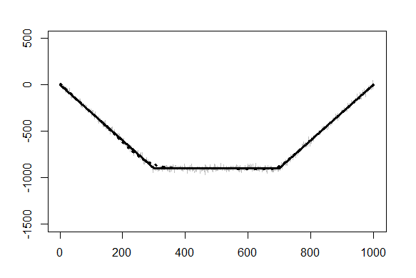
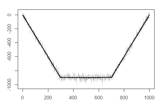
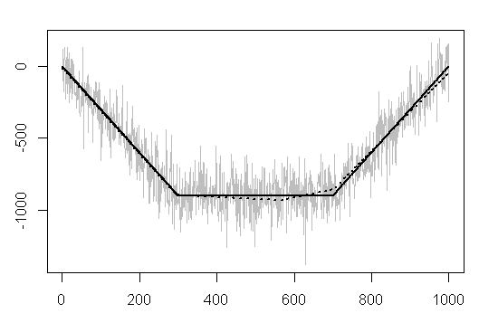
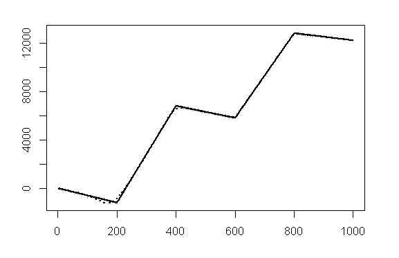
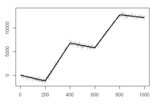
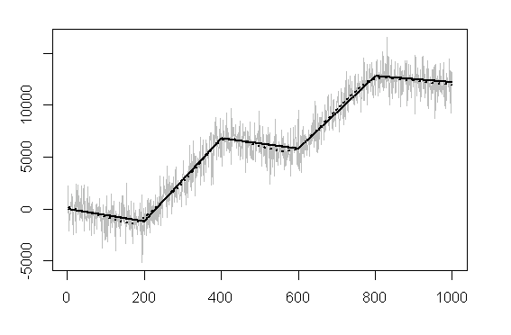
Figure 2: Simulated data examples for all six settings. $n=1000$. The solid curve is the underlying linear trend. The dotted curve is the LTF output for $\lambda=20a_{n}b_{\min}^{0}$. The low, moderate and heavy noises are plotted from the left to the right. The top and bottom panels are for Example 1 and 2, respectively.

We demonstrate the estimation effects by computing the relative error (RE) as follows:

$${\rm RE}(\widehat{\boldsymbol{\mu}}_{n},{\boldsymbol{\mu}}^{0})=\dfrac{\sum_{i=1}^{n}(\widehat{\mu}_{i}-\mu_{i}^{0})^{2}}{\sum_{i=1}^{n}\widehat{\mu}_{i}^{2}}.$$ (21)

To evaluate the performance of the $\ell_{1}$ trend filtering model in terms of the kink points recovery, we compute both means and standard deviations of the estimated kink point for all cases. Similar to Boysen et al. (2009) and Hrchaoui and Lévy-Leduc (2010), we also report the Hausorff distance between $\widehat{\cal J}$ and ${\cal J}^{0}$. Let $A$ and $B$ are two sets. The Hausdorff distance,

$${\rm HD}(A,B)=\sup\{{\cal E}(A||B);{\cal E}(B||A)\},$$ (22)

where ${\cal E}(A||B)=\sup_{b\in B}\inf_{a\in A}|a-b|$. We choose the optimal tuning parameter from $\lambda\in(0,\lambda_{\max})$ using both SIC in (19) and MC in (20), where $\lambda_{\max}$ is chosen to be the smallest one such as an affine fit is reached. The simulation results from Example 1 and 2 are summarized in Table 1.

Overall, MC works much better in terms of kink points detection. However, SIC generates less bias on mean estimation. In Figure 4 we plot both MC and SIC curves for a simulated data set generated from Example 2. The behavior of $\widehat{\boldsymbol{\mu}}(\lambda)$ depends on $\lambda$ tightly such that a larger $\lambda$ generates less kink points but trigger larger estimation biases, while a reasonable $\lambda$ for smaller bias may not be large enough for the recovery of underlying kink points. Such an observation is consistent with Comment 2 in Section 3.3. As a comparison, in Table 2, we also report some simulation results from the LASSO model (16). In general, the modified pathwise algorithm performs much better than the LASSO algorithm in terms of the kink point detection. The MC is used in both approaches.In Figure 3, we further review this phenomenon by plotting two estimated slope vector $\widehat{\boldsymbol{\nu}}$ from (12) and (16) for simulated data example in Example 1. We found that the $\widehat{\boldsymbol{\nu}}$ changes abruptly (Figure 3(a)) generated from the pathwise algorithm and model (12). However, $\widehat{\boldsymbol{\nu}}$ from the LASSO algorithm turns to change gradually around kink points (Figure 3(b)). It tells us that, even though both (12) and (16) are able to find a $\ell_{1}$ trend filter, the final solutions can be very different due to the different effects of the tuning parameter selection techniques.

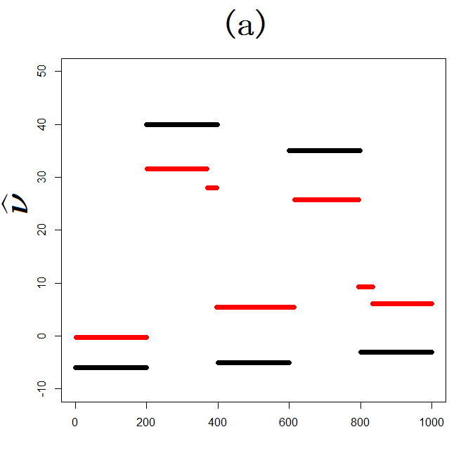
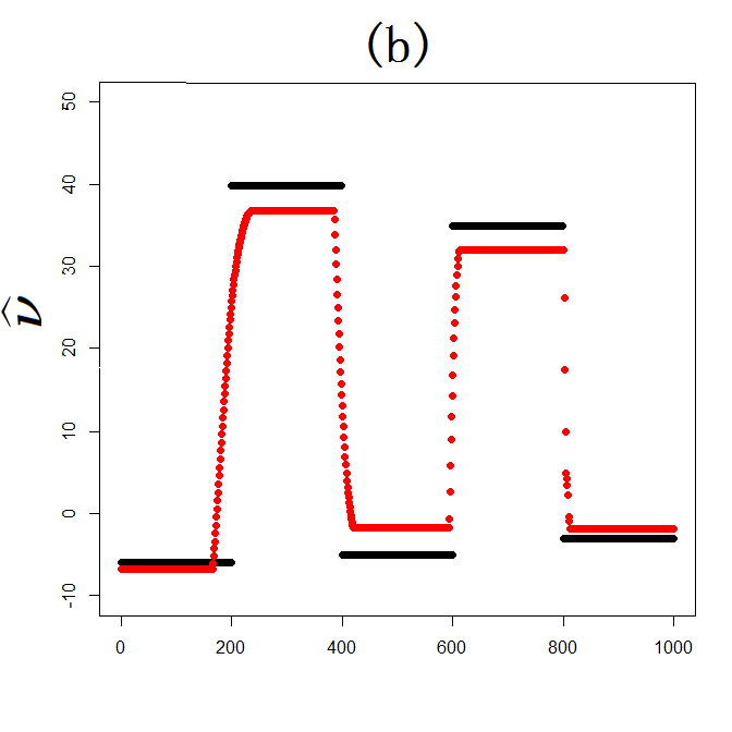
Figure 3: Fitted slope vector, $\widehat{\boldsymbol{\nu}}$, from a simulated data in Example 2. The left and right panels are outputs from pathwise decent algorithm for model (12) and coordinate decent algorithm for (16), respectively. (Observation: grey, True: black, SIC: blue, MC: red).

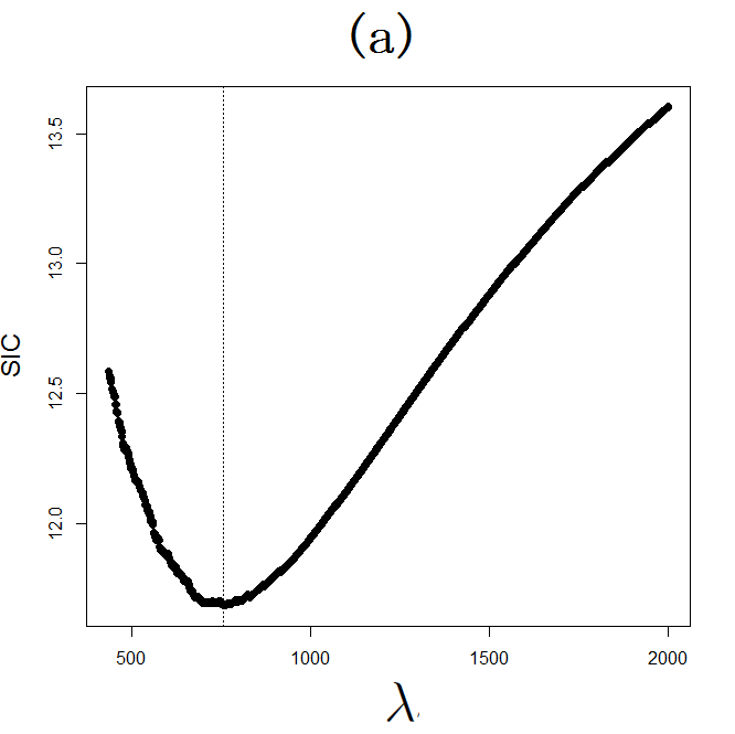
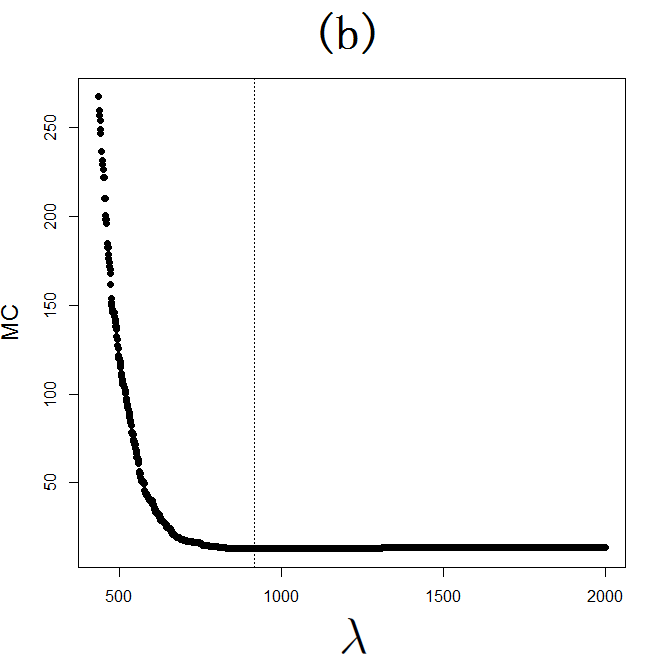
Figure 4: The SIC and MC curves for a simulated data with $n=1000$ with median noise in Example 2. Left: SIC; Right: MC. The vertical lines identify corresponding optimal $\lambda$ values

5 Discussion

In this paper, we study the asymptotic properties of the joint linear trend recovery using the $\ell_{1}$ regularization approach. By assuming the true model to be piece-wise linear, we investigate both the estimation consistency and sign consistency of an $\ell_{1}$ trend filter. In terms of estimation consistency, the consistency rate is optimal up to a logarithmic factor if the dimension of any linear space where the true model and its estimates belong to is bounded from above. In terms of sign consistency, we justify that an $\ell_{1}$ trend filter can not only recover the locations where the underlying linear pieces connect but also distinguish those slope changes in direction with high probability under reasonable conditions. Thus, by choosing the tuning parameter $\lambda$ properly, we can reach a well-behaved linear trend filter to recover the underlying linear piece-wise from some random noises. The consistency results in this paper amplify the study in Harchaoui and Lévy-Leduc (2010) and Rinaldo (2009), where the $\ell_{1}$ regularization approach is used to recover the piece-wise constant for signal approximation. As a by-product, we also justify that a weak irrepresentable condition is not necessary for the change point detection. In addition, we evaluate the performances of two alternative expressions of the $\ell_{1}$ trend filtering models in terms of both the total variation penalty and the LASSO penalty. A modified pathwise algorithm is preferred than the LASSO if the main focus is the kink points detection.

As in many recent studies for penalized regression, our results are proved for the penalty parameter that satisfy the conditions as stated in the theorems. It is not clear whether the penalty parameter selected using data-driven procedures satisfies those conditions. However, our numerical study shows a satisfactory finite-sample performance of the $\ell_{1}$ trend filter. Particularly, we note that the tuning parameter selected based on MC seems much better than the one from SIC for our simulated data. Tuning parameter selection is an important and challenging problem that requires further investigation, but is beyond the scope of the current paper.

6 Technical proofs

In this section, we provide proof of main results in Section 3. For the notation’s convenience, we sometimes omit $\lambda_{n}$ without causing any confusion.

Proof of Theorem 1

In this proof, we omit $\lambda_{n}$ and let $\widehat{\boldsymbol{\mu}}=\widehat{\boldsymbol{\mu}}(\lambda_{n})$ defined in (4). Recall that $\nu_{i}=\mu_{i}-\mu_{i-1}$ for $2\leq i\leq n$ and $\nu_{1}=\mu_{1}$. Then $\nu_{i}^{0}$ and $\widehat{\nu}_{i}$ are defined correspondingly. For example, $\widehat{\boldsymbol{\nu}}=(\widehat{\nu}_{1},\cdots,\widehat{\nu}_{n})^{\prime}$ with $\widehat{\nu}_{1}=\widehat{\mu}_{1}$ and $\widehat{\nu}_{i}=\widehat{\mu}_{i}-\widehat{\mu}_{i-1}$ for $2\leq i\leq n$. From the definition of $\widehat{\boldsymbol{\mu}}$ and $\widehat{\boldsymbol{\nu}}$, we have

$$(1/2)\sum_{i=1}^{n}\left(y_{i}-\sum_{j=1}^{i}\widehat{\nu}_{j}\right)^{2}+\lambda_{n}\sum_{i=2}^{n-1}|\widehat{\nu}_{i+1}-\widehat{\nu}_{i}|\leq(1/2)\sum_{i=1}^{n}\left(y_{i}-\sum_{j=1}^{i}\nu^{0}_{j}\right)^{2}+\lambda_{n}\sum_{i=2}^{n-1}|\nu^{0}_{i+1}-\nu^{0}_{i}|.$$

Then

$$(1/2)\sum_{i=1}^{n}\left[\sum_{j=1}^{i}(\widehat{\nu}_{j}-\nu_{j}^{0})\right]^{2}\leq\lambda_{n}[\sum_{i=1}^{n-1}|\nu^{0}_{i+1}-\nu^{0}_{i}|-|\widehat{\nu}_{i+1}-\widehat{\nu}_{i}|]+\sum_{i=1}^{n}[\sum_{j=1}^{i}(\widehat{\nu}_{j}-\nu^{0}_{j})\varepsilon_{i}].$$

Recall that ${\mathbf{x}}_{i}=(x_{1i},\cdots,x_{ni})^{\prime}$ for $1\leq i\leq n$ and ${\mathbf{X}}$ is a lower triangle matrix with $1$ for the non-zero element. We have

$$(1/2)(\widehat{\boldsymbol{\nu}}-{\boldsymbol{\nu}}^{0})^{\prime}\sum_{i=1}^{n}{\mathbf{x}}_{i}{\mathbf{x}}_{i}^{\prime}(\widehat{\boldsymbol{\nu}}-{\boldsymbol{\nu}}^{0})\leq 2\lambda_{n}\sum_{i=1}^{n}[|\widehat{\nu}_{i}-\nu_{i}^{0}|]+(\widehat{\boldsymbol{\nu}}-{\boldsymbol{\nu}}^{0})^{\prime}\sum_{i=1}^{n}{\mathbf{x}}_{i}\varepsilon_{i}.$$

and

$$(1/2)(\widehat{\boldsymbol{\nu}}-{\boldsymbol{\nu}}^{0})^{\prime}{\mathbf{X}}^{\prime}{\mathbf{X}}(\widehat{\boldsymbol{\nu}}-{\boldsymbol{\nu}}^{0})\leq 2\lambda_{n}n^{1/2}\|\widehat{\boldsymbol{\nu}}-{\boldsymbol{\nu}}^{0}\|_{2}+(\widehat{\boldsymbol{\nu}}-{\boldsymbol{\nu}}^{0})^{\prime}{\mathbf{X}}^{\prime}{\boldsymbol{\varepsilon}},$$

where ${\boldsymbol{\varepsilon}}=(\varepsilon_{1},\cdots,\varepsilon_{n})^{\prime}$. Denote $\Delta({\mathbf{w}})=\|X({\mathbf{w}}-{\boldsymbol{\nu}}^{0})\|_{2}$ and then $\Delta(\widehat{\boldsymbol{\nu}})=\|X(\widehat{\boldsymbol{\nu}}-{\boldsymbol{\nu}}^{0})\|_{2}$. Let $G({\mathbf{w}})=(\sigma\Delta({\mathbf{w}}))^{-1}({\mathbf{w}}-{\boldsymbol{\nu}}^{0})^{\prime}{\mathbf{X}}^{\prime}{\boldsymbol{\varepsilon}}$ for ${\mathbf{w}}\in{\cal R}^{n}$. Then we have

$$(1/2)(\Delta(\widehat{\boldsymbol{\nu}}))^{2}\leq 2\lambda_{n}n^{1/2}\|\widehat{\boldsymbol{\nu}}-{\boldsymbol{\nu}}^{0}\|_{2}+\sigma\Delta(\widehat{\boldsymbol{\nu}})G(\widehat{\boldsymbol{\nu}}).$$

Let $r_{1}\leq r_{2}\leq\cdots\leq r_{n}$ be $n$ eigenvalues of ${\mathbf{X}}^{\prime}{\mathbf{X}}$. Then $r_{1}>1/4$. Thus,

$$\Delta(\widehat{\boldsymbol{\nu}})\leq 16\lambda_{n}n^{1/2}+2\sigma G(\widehat{\boldsymbol{\nu}}).$$

So for any $\alpha_{n}>0$, we have

$$P\left(\Delta(\widehat{\boldsymbol{\nu}})\geq\alpha_{n}\right)\leq P\left(G(\widehat{\boldsymbol{\nu}})\geq\alpha_{n}/(2\sigma)-8\lambda_{n}n^{1/2}/\sigma\right).$$ (23)

We borrow some notations from Harchaoui and Lévy-Leduc (2010). Consider $\{S_{K}\}_{1\leq K\leq J^{0}}$ to be a collection of linear spaces where $\widehat{\boldsymbol{\nu}}$ may belong, where $S_{K}$ is a linear space of $K$ dimension. In addition, from Borell-TIS inequality (Ledoux and Talagrand, 1991), we have

$$P\left(\sup_{{\mathbf{w}}\in S_{K}}G({\mathbf{w}})\geq E[\sup_{{\mathbf{w}}\in S_{K}}G({\mathbf{w}})]+c\right)\leq\exp\{-c^{2}/2\}.$$ (24)

There exist an $n\times n$ orthogonal matrix ${\mathbf{P}}$ such that ${\mathbf{X}}^{\prime}{\mathbf{X}}={\mathbf{P}}^{\prime}{\boldsymbol{\Lambda}}{\mathbf{P}}$, where ${\boldsymbol{\Lambda}}=\hbox{diag}(r_{1},\cdots,r_{n})$ is a diagonal matrix. Let ${\cal W}$ be a $D$-dimensional linear space where ${\mathbf{w}}-{\boldsymbol{\nu}}^{0}$ belongs. Then we can write ${\mathbf{w}}-{\boldsymbol{\nu}}^{0}=\sum_{j=1}^{D}\alpha_{j}{\boldsymbol{\phi}}_{j}={\bf\Phi}{\boldsymbol{\alpha}}$, where ${\boldsymbol{\phi}}_{1},\cdots,{\boldsymbol{\phi}}_{D}$ are the orthogonal basis of ${\cal W}$, ${\bf\Phi}=({\boldsymbol{\phi}}_{1},\cdots,{\boldsymbol{\phi}}_{D})^{\prime}$ with ${\boldsymbol{\Phi}}^{\prime}{\boldsymbol{\Phi}}={\mathbf{I}}_{D}$ and, and ${\boldsymbol{\alpha}}=(\alpha_{1},\cdots,\alpha_{D})^{\prime}\in{\cal R}^{D}$. Define

$${\mathbf{b}}_{{\mathbf{a}}}{\mathbf{b}}_{{\mathbf{a}}}^{\prime}={\boldsymbol{\alpha}}^{\prime}{\boldsymbol{\Phi}}^{\prime}{\mathbf{X}}^{\prime}{\mathbf{X}}{\boldsymbol{\Phi}}{\boldsymbol{\alpha}}]^{-1/2}{\boldsymbol{\alpha}}^{\prime}{\boldsymbol{\Phi}}^{\prime}{\mathbf{X}}^{\prime}{\boldsymbol{\Phi}}.$$

From the Cauchy-Schwarz inequality, we have

$$\begin{array}[]{ll}\sigma E[\sup_{{\mathbf{w}}\in S_{K}}G({\mathbf{w}})]&=E[\sup_{{\boldsymbol{\alpha}}\in R^{D}}({\boldsymbol{\alpha}}^{\prime}{\boldsymbol{\Phi}}^{\prime}{\mathbf{X}}^{\prime}{\mathbf{X}}{\boldsymbol{\Phi}}{\boldsymbol{\alpha}})^{-1/2}{\boldsymbol{\alpha}}^{\prime}{\boldsymbol{\Phi}}^{\prime}{\mathbf{X}}^{\prime}{\boldsymbol{\varepsilon}}]\\ &=E[\sup_{{\boldsymbol{\alpha}}\in R^{D}}{\mathbf{b}}_{{\mathbf{a}}}^{\prime}{\boldsymbol{\Phi}}^{\prime}{\boldsymbol{\varepsilon}}]\\ &\leq\sup_{{\boldsymbol{\alpha}}\in R^{D}}\{({\mathbf{b}}_{{\mathbf{a}}}^{\prime}{\mathbf{b}}_{{\mathbf{a}}})^{1/2}E[({\boldsymbol{\varepsilon}}^{\prime}{\boldsymbol{\Phi}}{\boldsymbol{\Phi}}^{\prime}{\boldsymbol{\varepsilon}})^{1/2}]\}.\end{array}$$ (28)

First,

$$E[{\boldsymbol{\varepsilon}}^{\prime}{\boldsymbol{\Phi}}{\boldsymbol{\Phi}}^{\prime}{\boldsymbol{\varepsilon}}]=\sigma^{2}{\rm tr}({\boldsymbol{\Phi}}{\boldsymbol{\Phi}}^{\prime})=\sigma^{2}{\rm tr}({\boldsymbol{\Phi}}^{\prime}{\boldsymbol{\Phi}})\leq D\sigma^{2}.$$

We will prove that $\sup_{{\boldsymbol{\alpha}}\in R^{D}}({\mathbf{b}}_{{\mathbf{a}}}^{\prime}{\mathbf{b}}_{{\mathbf{a}}})^{1/2}\leq 1$ as follows

$$\begin{array}[]{ll}{\mathbf{b}}_{{\mathbf{a}}}^{\prime}{\mathbf{b}}_{{\mathbf{a}}}-1&=({\boldsymbol{\alpha}}^{\prime}{\bf\Phi}^{\prime}{\mathbf{X}}^{\prime}{\mathbf{X}}{\bf\Phi}{\boldsymbol{\alpha}})^{-1}({\boldsymbol{\alpha}}^{\prime}{\boldsymbol{\Phi}}^{\prime}{\mathbf{X}}^{\prime}{\boldsymbol{\Phi}}{\boldsymbol{\Phi}}^{\prime}{\mathbf{X}}{\boldsymbol{\Phi}}{\boldsymbol{\alpha}})-1\\ &=({\boldsymbol{\alpha}}^{\prime}{\bf\Phi}^{\prime}{\mathbf{X}}^{\prime}{\mathbf{X}}{\bf\Phi}{\boldsymbol{\alpha}})^{-1}[{\boldsymbol{\alpha}}^{\prime}{\boldsymbol{\Phi}}^{\prime}{\mathbf{X}}^{\prime}({\boldsymbol{\Phi}}{\boldsymbol{\Phi}}^{\prime}-{\mathbf{I}}_{n}){\mathbf{X}}{\boldsymbol{\Phi}}{\boldsymbol{\alpha}}]\end{array}$$

Notice that ${\mathbf{I}}_{n}-{\boldsymbol{\Phi}}{\boldsymbol{\Phi}}^{\prime}\geq 0$ is an idempotent semi-definite matrix. Eigenvalues of ${\boldsymbol{\Phi}}{\boldsymbol{\Phi}}^{\prime}-{\mathbf{I}}_{n}$ are only $0$ and $-1$. Therefore, ${\mathbf{b}}_{{\mathbf{a}}}^{\prime}{\mathbf{b}}_{{\mathbf{a}}}-1\leq 0$ and ${\mathbf{b}}_{{\mathbf{a}}}^{\prime}{\mathbf{b}}_{{\mathbf{a}}}^{1/2}\leq 1$. Thus from (28),

$$E[\sup_{{\mathbf{w}}\in S_{K}}G({\mathbf{w}})]\leq D^{1/2}\leq(2J_{\max})^{1/2}.$$ (29)

From (29), we have

$$d_{K} \equiv\alpha_{n}/(2\sigma)-8\lambda_{n}n^{1/2}/\sigma-E[\sup_{{\mathbf{w}}\in S_{K}}G({\mathbf{w}})]$$ (30)

$$>\alpha_{n}/(2\sigma)-8\lambda_{n}n^{1/2}/\sigma-(2J_{\max})^{1/2}.$$ (31)

We denote $c_{0}=\alpha_{n}/(2\sigma)-8\lambda_{n}n^{1/2}/\sigma-(2J_{\max})^{1/2}$. Then if we choose $\alpha_{n}$ such that $\alpha_{n}/(2\sigma)-8\lambda_{n}n^{1/2}/\sigma-(2J_{\max})^{1/2}>0$ is satisfied. Then there exists $0<A<1$, such that

$$A\alpha_{n}/(2\sigma)=8\lambda_{n}n^{1/2}/\sigma+(2J_{\max})^{1/2}.$$

If we define

$$c_{0}=(1-A)\alpha_{n}/\sigma,$$ (32)

then $d_{K}>c_{0}>0$. From (23) and (32), we have

$$\begin{array}[]{ll}P\left(\Delta(\widehat{\boldsymbol{\nu}})\geq\alpha_{n}\right)&\leq\sum_{K=1}^{J_{\max}}n^{K}P\left(\sup_{{\mathbf{w}}\in S_{K}}G({\mathbf{w}})\geq\alpha_{n}/(2\sigma)-8\lambda_{n}n^{1/2}/\sigma\right)\\ &=\sum_{K=1}^{J_{\max}}n^{K}P\left(\sup_{{\mathbf{w}}\in S_{K}}G({\mathbf{w}})\geq E[\sup_{{\mathbf{w}}\in S_{K}}|G({\mathbf{w}})|]+d_{K}\right)\\ &\leq J_{\max}n^{J_{\max}}P\left(\sup_{{\mathbf{w}}\in S_{K}}G({\mathbf{w}})\geq E[\sup_{{\mathbf{w}}\in S_{K}}|G({\mathbf{w}})|]+c_{0}\right)\\ &\leq J_{\max}n^{J_{\max}}\exp\{-c_{0}^{2}\}\\ &=J_{\max}\exp\{J_{\max}\log n-[(\alpha_{n}/\sigma)(1-A)]^{2}\}.\end{array}$$

Let $(\alpha_{n}/(2\sigma))^{2}=J_{\max}B\log n$ and then $\alpha_{n}=2\sigma(J_{\max}B\log n)^{1/2}$. Thus, we have

$$\begin{array}[]{ll}&P\left(n^{-1/2}\|\widehat{\boldsymbol{\mu}}-{\boldsymbol{\mu}}^{0}\|\geq\sigma(J_{\max}B(\log n)/n)^{1/2}\right)\\ &\quad=P(\Delta(\widehat{\boldsymbol{\nu}})\geq\alpha_{n})\\ &\quad\leq J_{\max}\exp\{J_{\max}\log n-BJ_{\max}(\log n)(1-A)^{2}\}\\ &\quad=J_{\max}\exp\{J_{\max}(\log n)(1-B(1-A)^{2}/2)\}\\ &\quad=J_{\max}n^{J_{\max}[1-B(1-A)^{2}/2]}\to 0~{}{\rm if}~{}B>2/(1-A)^{2}.\end{array}$$

$\Box$

Proof of Theorem 2

Let ${\mathbf{a}}=(a_{1},\cdots,a_{J+1})^{\prime}$ and ${\bf b}=(b_{1},\cdots,b_{J+1})^{\prime}$, where $(a_{j},b_{j})$ is the intercept and slope of the $j$th local linear pieces. For linear model (1–3), we can write the penalized loss function in (5) into

$$f({\mathbf{a}},{\bf b};\lambda_{n})=(1/2)\sum_{j=1}^{J+1}\sum_{k\in{\cal B}_{j}}(y_{k}-(a_{j}+b_{j}k))^{2}+\lambda_{n}\sum_{j=2}^{J+1}|b_{j}-b_{j-1}|.$$ (33)

Suppose $\widehat{\mathbf{a}}(\lambda_{n})$ and $\widehat{\bf b}(\lambda_{n})$ are the optimizer of (33) for $\lambda_{n}>0$. We omitted $\lambda_{n}$ for the rest of the proof without causing any confusion. Let $\widehat{\cal B}_{j(i)}$ represent the index set of the local linear segment where $\widehat{\mu}_{i}$ stays. Correspondingly, $(\widehat{a}_{j(i)},\widehat{b}_{j(i)})^{\prime}s$ are the local intercept and slopes at $i$ and $\widehat{\mu}_{i}=\widehat{a}_{j(i)}+\widehat{b}_{j(i)}i$ for $1\leq i\leq n$. From the Karush-Kuhn-Tucker condition of the above optimization problem (33), $\widehat{\boldsymbol{\mu}}$ is an LTF solution if and only if

$$\left\{\begin{array}[]{ll}\sum_{k\in\widehat{\cal B}_{j(i)}}k[y_{k}-(\widehat{a}_{j(i)}+\widehat{b}_{j(i)}k)]=\lambda_{n}\widehat{c}_{j(i)}&\quad{\rm for~{}}\widehat{b}_{j(i)}\neq\widehat{b}_{j(i-1)}\\ \arrowvert\sum_{k\in\widehat{\cal B}_{j(i)}}k[y_{k}-(\widehat{a}_{j(i)}+\widehat{b}_{j(i)}k)]\arrowvert<4\lambda_{n}&\quad{\rm for~{}}\widehat{b}_{j(i)}=\widehat{b}_{j(i-1)}\end{array}\right.,$$ (36)

where $\widehat{b}_{j(i)}=\widehat{b}_{j(i-1)}$ also means $\widehat{\mu}_{i}-\widehat{\mu}_{i-1}=\widehat{\mu}_{i+1}-\widehat{\mu}_{i}$. Here $\widehat{c}_{j(i)}$ is an corresponding estimation of $c_{j}$ in (9). Define ${\boldsymbol{\gamma}}_{j(i)}\equiv(\sum_{k\in{\cal B}_{j(i)}^{0}}k,\sum_{k\in{\cal B}_{j(i)}^{0}}k^{2})^{\prime}$. Consider

$$\widehat{a}_{j(i)}=a^{0}_{j(i)}++({\boldsymbol{\gamma}}_{j(i)}^{\prime}{\boldsymbol{\gamma}}_{j(i)})^{-1}\left(\sum_{k\in{\cal B}_{j(i)}^{0}}k\right)\left(\sum_{l\in{\cal B}_{j(i)}^{0}}l\varepsilon_{l}-\lambda_{n}c_{j(i)}^{0}\right)~{}{\rm for~{}}i\in{\cal J}^{0},$$ (37)

and

$$\widehat{b}_{j(i)}=b^{0}_{j(i)}+({\boldsymbol{\gamma}}_{j(i)}^{\prime}{\boldsymbol{\gamma}}_{j(i)})^{-1}\left(\sum_{k\in{\cal B}_{j(i)}^{0}}k^{2}\right)\left(\sum_{l\in{\cal B}_{j(i)}^{0}}l\varepsilon_{l}-\lambda_{n}c_{j(i)}^{0}\right)~{}{\rm for~{}}i\in{\cal J}^{0}.$$ (38)

Thus $\widehat{\bf b}$ satisfying (38) and

$$\widehat{b}_{j(i)}=\widehat{b}_{j(i-1)},\quad i\notin{\cal J}^{0}$$ (39)

is a solution of ${\bf b}$ in (33). Therefore, from (36), ${\cal S}^{n}$ holds if and only if $\widehat{\bf b}$ in (38–39) satisfies

$$\mbox{sgn}(\widehat{b}_{j(i)}-\widehat{b}_{j(i-1)})=\mbox{sgn}(b^{0}_{j(i)}-b^{0}_{j(i-1)}) \quad{\rm for~{}}i\in{\cal J}^{0}$$ (40)

and

$$\arrowvert\sum_{k\in\widehat{B}^{0}_{j(i)}}k[y_{k}-(\widehat{a}_{j(i)}+\widehat{b}_{j(i)}k)]\arrowvert<2\lambda_{n} \quad{\rm for~{}}\widehat{b}_{j(i)}=\widehat{b}_{j(i-1)}.$$ (41)

We now first verify (40). Notice that (40) holds if

$$|(\widehat{b}_{j(i)}-b^{0}_{j(i)})-(\widehat{b}_{j(i-1)}-b^{0}_{j(i-1)})|<|b^{0}_{j(i)}-b^{0}_{j(i-1)}| \quad{\rm for~{}}i\in{\cal J}^{0}.$$ (42)

Plug (38) into (42), we get

$$\begin{array}[]{ll}&\vline\left[({\boldsymbol{\gamma}}_{j(i)}^{\prime}{\boldsymbol{\gamma}}_{j(i)})^{-1}\sum_{k\in{\cal B}_{j(i)}^{0}}k^{2}\left(\sum_{l\in{\cal B}_{j(i)}^{0}}l\varepsilon_{l}-\lambda_{n}c_{j(i)}^{0}\right)\right]-\\ &\quad\left[({\boldsymbol{\gamma}}_{j(i-1)}^{\prime}{\boldsymbol{\gamma}}_{j(i-1)})^{-1}\sum_{k\in{\cal B}_{j(i-1)}^{0}}k^{2}\left(\sum_{l\in{\cal B}_{j(i-1)}^{0}}l\varepsilon_{l}-\lambda_{n}c_{j(i-1)}^{0}\right)\right]\vline\\ &\quad\quad<|b^{0}_{j(i)}-b^{0}_{j(i-1)}|\quad{\rm for~{}}i\in{\cal J}^{0}.\end{array}$$ (43)

Notice that $a_{n}=\min_{i\in{\cal J}^{0}}|b^{0}_{j(i)}-b^{0}_{j(i-1)}|$. We expand (43) into different inequalities. Denote $I_{1}$ as

$$\left\{\max_{i\in{\cal J}^{0}}\left|({\boldsymbol{\gamma}}_{j(i)}^{\prime}{\boldsymbol{\gamma}}_{j(i)})^{-1}\sum_{k\in{\cal B}_{j(i)}^{0}}k^{2}\sum_{l\in{\cal B}_{j(i)}^{0}}l\varepsilon_{l}-({\boldsymbol{\gamma}}_{j(i-1)}^{\prime}{\boldsymbol{\gamma}}_{j(i-1)})^{-1}\sum_{k\in{\cal B}_{j(i-1)}^{0}}k^{2}\sum_{l\in{\cal B}_{j(i-1)}^{0}}l\varepsilon_{l}\right|\leq a_{n}/2\right\}.$$ (44)

Denote $I_{2}=I_{21}\cap I_{22}$ and

$$\begin{array}[]{ll}I_{21}&\equiv\left\{\max_{i\in{\cal J}^{0}}\left|({\boldsymbol{\gamma}}_{j(i)}^{\prime}{\boldsymbol{\gamma}}_{j(i)})^{-1}\sum_{k\in{\cal B}_{j(i)}^{0}}k^{2}c_{j(i)}^{0}\right|\leq a_{n}/(2\lambda_{n})\right\}\\ I_{22}&\equiv\left\{\max_{i\in{\cal J}^{0}}\left|({\boldsymbol{\gamma}}_{j(i-1)}^{\prime}{\boldsymbol{\gamma}}_{j(i-1)})^{-1}\sum_{k\in{\cal B}_{j(i-1)}^{0}}k^{2}c_{j(i-1)}^{0}\right|\leq a_{n}/(2\lambda_{n})\right\}.\end{array}$$ (45)

Therefore (43) holds if $I_{1}$, $I_{21}$ and $I_{22}$ hold. If (B1) holds, then

$$\frac{\lambda_{n}}{a_{n}}<\sum_{k\in{\cal B}_{j(i)}^{0}}k<\frac{1}{2}\left(\frac{\left(\sum_{k\in{\cal B}_{j(i)}^{0}}k\right)^{2}}{\sum_{k\in{\cal B}_{j(i)}^{0}}k^{2}}+\sum_{k\in{\cal B}_{j(i)}^{0}}k^{2}\right)=\left(2({\boldsymbol{\gamma}}_{j(i)}^{\prime}{\boldsymbol{\gamma}}_{j(i)})^{-1}\sum_{k\in{\cal B}_{j(i)}^{0}}k^{2}\right)^{-1}.$$

Thus

$$P(I_{2}^{c})\leq P(I_{21})+P(I_{22})=0.$$ (46)

We now consider the event $I_{1}$. Let

$$\tau_{i}=({\boldsymbol{\gamma}}_{j(i)}^{\prime}{\boldsymbol{\gamma}}_{j(i)})^{-1}\sum_{k\in{\cal B}_{j(i)}^{0}}k^{2}\sum_{l\in{\cal B}_{j(i)}^{0}}\varepsilon_{l}-({\boldsymbol{\gamma}}_{j(i-1)}^{\prime}{\boldsymbol{\gamma}}_{j(i-1)})^{-1}\sum_{k\in{\cal B}_{j(i-1)}^{0}}k^{2}\sum_{l\in{\cal B}_{j(i-1)}^{0}}\varepsilon_{l}.$$

Then $E[\tau_{i}]=0$ and ${\bf\hbox{Var}}[\tau_{i}]\leq 2\Delta^{2}$, where

$$\Delta^{2}=\max_{i\in{\cal J}^{0}}\left\{\left[({\boldsymbol{\gamma}}_{j(i)}^{\prime}{\boldsymbol{\gamma}}_{j(i)})^{-1}\sum_{k\in{\cal B}_{j(i)}^{0}}k^{2}\right]^{2}\sum_{l\in{\cal B}_{j(i)}^{0}}l^{2}\right\}.$$ (47)

Consider independent copies $\tau_{i}^{*}\sim N(0,2\Delta^{2})$. From (44) and the Slepian inequality, we have

$$P(I_{1}^{c})=P(\max_{i\in{\cal J}_{0}}|\tau_{i}|>\frac{a_{n}}{2})\leq P(\max_{i\in{\cal J}_{0}}|\tau_{i}^{*}|>\frac{a_{n}}{2})\leq\exp\{-\frac{a_{n}^{2}}{8\Delta^{2}}\}.$$ (48)

From (47), we know

$$\Delta^{2}=\max_{i\in{\cal J}_{0}}\left[\frac{\left(\sum_{k\in{\cal B}_{j(i)}^{0}}k^{2}\right)^{3/2}}{\left(\sum_{k\in{\cal B}_{j(i)}^{0}}k\right)^{2}+\left(\sum_{k\in{\cal B}_{j(i)}^{0}}k^{2}\right)^{2}}\right]^{2}\leq\max_{i\in{\cal J}_{0}}\left(\sum_{k\in{\cal B}_{j(i)}^{0}}k^{2}\right)^{-1}\leq 3/(b_{\min}^{0})^{3}.$$

The last “$\leq$” is because $\sum_{k\in{\cal B}_{j(i)}^{0}}k^{2}\leq|{\cal B}_{j(i)}^{0}|^{3}/3$. Thus $P(I_{1}^{c})=0$ from (B2). Combining with (46), we know that (40) holds with probability to $1$ when $n\to\infty$. In order to verify (41), we consider the sub-differential on ${\boldsymbol{\mu}}$ vector,

$$y_{k}-\widehat{\mu}_{k}=\varepsilon_{k}-(\widehat{\mu}_{k}-\mu_{k}^{0})=\lambda_{n}(\widehat{h}_{k})~{}{\rm for~{}}3\leq k\leq n,$$ (49)

where $\widehat{h}_{k}=-2\mbox{sgn}(\widehat{\mu}_{k-1}+\widehat{\mu}_{k+1}-2\widehat{\mu}_{k})+\mbox{sgn}(\widehat{\mu}_{k-2}+\widehat{\mu}_{k}-2\widehat{\mu}_{k-1})+\mbox{sgn}(\widehat{\mu}_{k}+\widehat{\mu}_{k+2}-2\widehat{\mu}_{k+1})$ for $3\leq k\leq n-2$, $\widehat{h}_{n}=\mbox{sgn}(\widehat{\mu}_{n-2}+\widehat{\mu}_{n}-2\widehat{\mu}_{n-1})$ and $\widehat{h}_{n-1}=-2\mbox{sgn}(\widehat{\mu}_{n-2}+\widehat{\mu}_{n}-2\widehat{\mu}_{n-1})+\mbox{sgn}(\widehat{\mu}_{n-3}+\widehat{\mu}_{n-1}-2\widehat{\mu}_{n-2}).$ If we apply (49) to $k=i-1,i$ and $i+1$ separately and then we get

$$\varepsilon_{i+1}+\varepsilon_{i-1}-2\varepsilon_{i}-[(\widehat{\mu}_{i+1}+\widehat{\mu}_{i-1}-2\widehat{\mu}_{i})-(\mu^{0}_{i+1}+\mu^{0}_{i-1}-2\mu^{0}_{i})]=\lambda_{n}[\widehat{h}_{i+1}+\widehat{h}_{i-1}-2\widehat{h}_{i}].$$

In fact, $\widehat{b}_{j(i)}=\widehat{b}_{j(i-1)}$, or equivalently $i\notin{\cal J}^{0}$, means $\widehat{\mu}_{i+1}+\widehat{\mu}_{i-1}-2\widehat{\mu}_{i}=\mu^{0}_{i+1}+\mu^{0}_{i-1}-2\mu^{0}_{i}=0$. Then we (41) holds if

$$|\varepsilon_{i+1}+\varepsilon_{i-1}-2\varepsilon_{i}|\leq 14\lambda_{n}\quad{\rm for~{}}i\notin{\cal J}^{0}.$$

Denote $d_{i}^{{\boldsymbol{\varepsilon}}}=\varepsilon_{i+1}/\sqrt{6}+\varepsilon_{i-1}/\sqrt{6}-2\varepsilon_{i}/\sqrt{6}$. From (A1), $d_{i}^{{\boldsymbol{\varepsilon}}}$ has sub-Gaussian distribution with mean $0$ and variance $\sigma^{2}$. Then

$$E[\max_{i\notin{\cal J}^{0}}|d_{i}^{{\boldsymbol{\varepsilon}}}|]\leq\frac{\sigma(2+\log(n-|{\cal J}^{0}|))}{2}.$$ (50)

If $14\lambda_{n}-(\sigma/2)(2+\log(n-|{\cal J}^{0}|))>0$, then from (50), we have

$$\begin{array}[]{ll}P(\max_{i\notin{\cal J}^{0}}|d_{i}^{{\boldsymbol{\varepsilon}}}|>14\lambda_{n})&\leq\exp\{-[14\lambda_{n}-(\sigma/2)(2+\log(n-|{\cal J}^{0}|))]^{2}/2\\ &=\exp\{-(14\lambda_{n})^{2}[1-(\sigma/28)((2+\log(n-|{\cal J}^{0}|))/\lambda_{n})]^{2}/2\\ &\leq\exp\{-(14\lambda_{n})^{2}(1-\delta))^{2}\},\end{array}$$ (51)

where the first “$\leq$” is from the Borell-TIS inequality and the second “$\leq$” is from (B3-b). Denote $I_{3}\equiv\{\max_{i\notin{\cal J}^{0}}|d_{i}^{{\boldsymbol{\varepsilon}}}|<14\lambda_{n}\}$. Then $P(I_{3}^{c})\to 0$ if (B3-a) holds. Thus $\lim_{n\to\infty}P({\cal S}^{n})\geq 1-(P(I_{1}^{c})+P(I_{2}^{c})+P(I_{3}^{c}))=1.$ $\Box$

A counter-example for weak irrepresentable condition in Section 3.3

Specifically, the design matrix of model (16) is

$${\mathbf{Z}}=\begin{pmatrix}1&&&&&&\\ 1&1&&&&&\\ 1&2&1&&&&\\ 1&3&2&1&&&\\ \vdots&\vdots&\vdots&\vdots&\ddots&1&\\ 1&n-1&n-2&n-3&\cdots&2&1\end{pmatrix}.$$

Suppose $t_{1}^{0}<t_{2}^{0}<\cdots<t_{J}^{0}$ are all true kink points. Denote $d^{n_{k}}=\sum_{i=1}^{n_{k}}i$ and $d^{n_{k}}_{l,m}=\sum_{i=1}^{n_{k}}i(i+t_{j_{m}}-t_{j_{l}})$ with $n_{k}=n-(t_{k}-1)$ for $1\leq k,l,m\leq J$. We can write ${\mathbf{Z}}_{{\mathbf{1}}}^{\prime}{\mathbf{Z}}_{{\mathbf{1}}}$ explicitly. We as follows,

$${\mathbf{Z}}_{{\mathbf{1}}}^{\prime}{\mathbf{Z}}_{{\mathbf{1}}}=\begin{pmatrix}n&d^{n_{1}}&d^{n_{2}}&d^{n_{3}}&\cdots&d^{n_{J-1}}&d^{n_{J}}\\ d^{n_{1}}&d^{n_{1}}_{1,1}&d^{n_{2}}_{1,2}&d^{n_{3}}_{1,3}&\cdots&d^{n_{J-1}}_{1,J-1}&d^{n_{J}}_{1,J}\\ d^{n_{2}}&d^{n_{2}}_{1,2}&d^{n_{2}}_{2,2}&d^{n_{3}}_{2,3}&\cdots&d^{n_{J-1}}_{2,J-1}&d^{n_{J}}_{2,J}\\ d^{n_{3}}&d^{n_{3}}_{1,3}&d^{n_{3}}_{2,3}&d^{n_{3}}_{3,3}&\cdots&d^{n_{J-1}}_{3,J-1}&d^{n_{J}}_{3,J}\\ \vdots&\vdots&\vdots&\vdots&\ddots&\vdots&\vdots\\ d^{n_{J-1}}&d^{n_{J-1}}_{1,J-1}&d^{n_{J-1}}_{2,J-1}&d^{n_{J-1}}_{3,J-1}&\cdots&d^{n_{J-1}}_{J-1,J-1}&d^{n_{J}}_{J-1,J}(i)\\ d^{n_{J}}&d^{n_{J}}_{1,J}&d^{n_{J}}_{2,J}&d^{n_{J}}_{3,J}&\cdots&d^{n_{J}}_{J-1,J}&d^{n_{J}}_{J,J}\end{pmatrix}.$$

Here $t_{1}=2$ since there is no penalty on $\beta_{1}$ and $\beta_{2}$, both ${\mathbf{z}}_{1}$ and ${\mathbf{z}}_{2}$ are included in ${\mathbf{Z}}_{{\mathbf{1}}}$. Suppose there is only one counter example $t_{1}$.

$${\mathbf{Z}}_{{\mathbf{1}}}^{\prime}{\mathbf{Z}}_{{\mathbf{1}}}=\begin{pmatrix}n&\sum_{i=1}^{n-1}i&\sum_{i=1}^{n-t_{1}+1}i\\ \sum_{i=1}^{n-1}i&\sum_{i=1}^{n-1}i^{2}&\sum_{i=1}^{n-t_{1}+1}i(i+t_{1}-2)\\ \sum_{i=1}^{n-t_{1}+1}i&\sum_{i=1}^{n-t_{1}+1}i(i+t_{1}-2)&\sum_{i=1}^{n-t_{1}+1}i^{2}\end{pmatrix}.$$

Without loss of generalicity, we let $n=10$, $t_{1}=5$. Then the seven 3-d vectors in ${\mathbf{Z}}^{\prime}_{{\mathbf{2}}}{\mathbf{Z}}_{{\mathbf{1}}}({\mathbf{Z}}^{\prime}_{{\mathbf{1}}}{\mathbf{Z}}_{{\mathbf{1}}})^{-1}$ are ${\mathbf{a}}_{1}=(-0.3255,0.7383,0.2872)^{\prime}$, ${\mathbf{a}}_{2}=(-0.2383,0.3574,0.6809)$, ${\mathbf{a}}_{3}=(0.1277,-0.1915,1.0638)^{\prime}$ ${\mathbf{a}}_{4}=(0.1702,-0.2553,0.9422)^{\prime}$, ${\mathbf{a}}_{5}=(0.1532,-0.2298,0.7052)^{\prime}$, ${\mathbf{a}}_{6}=(0.1021,-0.1532,0.4225)^{\prime}$ and ${\mathbf{a}}_{7}=(0.0426,-0.0638,0.1641)^{\prime}$. If ${\mathbf{s}}_{{\mathbf{1}}}=(1,1,1)^{\prime}$, then $|{\mathbf{a}}_{j}^{\prime}{\mathbf{s}}_{{\mathbf{1}}}|=1$ for $j=3$. If ${\mathbf{s}}_{{\mathbf{1}}}=(1,-1,1)^{\prime}$, then $|{\mathbf{a}}_{j}^{\prime}{\mathbf{s}}_{{\mathbf{1}}}|>1$ for $j=3,4,5$. If ${\mathbf{s}}_{{\mathbf{1}}}=(1,1,-1)^{\prime}$, then $|{\mathbf{a}}_{j}^{\prime}{\mathbf{s}}_{{\mathbf{1}}}|>1$ for $j=3,4$. If ${\mathbf{s}}_{{\mathbf{1}}}=(-1,1,1)^{\prime}$, then $|{\mathbf{a}}_{j}^{\prime}{\mathbf{s}}_{{\mathbf{1}}}|>1$ for $j=1,2$.$\Box$

Table 1: Simulation results using SIC and MC for Example 1 and 2 in Section 4.2.

			$n=500$				$n=1000$
			Low	Medium	High		Low	Medium	High
Example 1 ($k=3$)
		RE	0.000	0.002	0.039		0.000	0.002	0.047
			(0.000)	(0.003)	(0.089)		(0.000)	(0.003)	(0.141)
		$|{\cal J}|$	20.83	31.14	41.19		44.12	14.42	10.59
			(76.365)	(105.807)	(125.186)		(166.980)	(7.643)	(6.612)
	SIC	eAB	0.003	0.009	0.030		0.002	0.008	0.029
			(0.002)	(0.006)	(0.022)		(0.001)	(0.005)	(0.019)
		eBA	0.286	0.261	0.249		0.275	0.255	0.239
			(0.013)	(0.049)	(0.059)		(0.032)	(0.056)	(0.067)
		RE	0.000	0.003	0.058		0.000	0.003	0.069
			(0.000)	(0.004)	(0.134)		(0.000)	(0.005)	(0.177)
		$|{\cal J}|$	3.54	3.66	3.68		8.01	7.55	5.41
			(1.009)	(1.094)	(1.034)		(1.811)	(1.855)	(1.450)
	MC	eAB	0.003	0.009	0.034		0.002	0.009	0.032
			(0.002)	(0.006)	(0.023)		(0.001)	(0.005)	(0.020)
		eBA	0.275	0.243	0.231		0.256	0.213	0.205
			(0.028)	(0.055)	(0.061)		(0.045)	(0.064)	(0.076)
Example 2 ($k=5$)
		RE	0.015	0.009	0.037		0.018	0.015	0.034
			(0.000)	(0.003)	(0.047)		(0.001)	(0.003)	(0.044)
		$|{\cal J}|$	5.89	7.07	11.25		5.38	6.28	13.48
			(1.377)	(1.565)	(4.368)		(1.099)	(1.341)	(5.668)
	SIC	eAB	0.003	0.010	0.033		0.003	0.009	0.031
			(0.001)	(0.005)	(0.018)		(0.001)	(0.005)	(0.021)
		eBA	0.186	0.038	0.165		0.005	0.027	0.178
			(0.042)	(0.025)	(0.036)		(0.003)	(0.015)	(0.023)
		RE	0.016	0.011	0.047		0.019	0.015	0.047
			(0.002)	(0.005)	(0.056)		(0.001)	(0.004)	(0.051)
		$|{\cal J}|$	5.38	6.03	6.48		5.13	5.87	5.53
			(1.022)	(1.344)	(1.629)		(0.884)	(1.088)	(1.322)
	MC	eAB	0.013	0.012	0.049		0.003	0.011	0.055
			(0.043)	(0.019)	(0.043)		(0.001)	(0.019)	(0.053)
		eBA	0.186	0.033	0.133		0.005	0.026	0.132
			(0.042)	(0.023)	(0.050)		(0.003)	(0.015)	(0.055)
NOTE 1: RE is the relative error defined in (21).
NOTE 2: eAB and eBA are ${\cal E}(A,B)$ and ${\cal E}(B,A)$ in (22) divided by $n$.
NOTE 2: $|{\cal J}|$ is defined estimated kink points number.
NOTE 3: Values in the parenthesis are for corresponding standard deviations.

Table 2: LASSO output using MC for Example 1 and 2 with $n=1000$ in Section 4.2.

	Example 1 ($k=3$)				Example 2 ($k=5$)
	Low	Medium	High		Low	Medium	High
RE	0.024	0.036	1.085		1e-4	1e-4	0.001
	(0.003)	(0.011)	(0.289)		(1e-5)	(1e-5)	(1e-6)
$|{\cal J}|$	42.16	41.38	51.94		91.26	92.56	96.04
	(1.434)	(4.899)	(14.816)		(0.443)	(3.494)	(1.470)
eAB	0.000	0.000	0.001		0.000	0.001	0.014
	(0.000)	(0.000)	(0.002)		(0.000)	(0.001)	(0.000)
eBA	0.067	0.099	0.293		0.032	0.032	0.036
	(0.019)	(0.053)	(0.003)		(0.000)	(0.002)	(0.000)
NOTE 1: RE is the relative error defined in (21).
NOTE 2: eAB and eBA are ${\cal E}(A,B)$ and ${\cal E}(B,A)$ in (22) divided by $n$.
NOTE 3: $|{\cal J}|$ is defined estimated kink points number.
NOTE 4: Values in the parenthesis are for corresponding standard deviations.