Competition between Born solvation, dielectric exclusion, and Coulomb attraction in spherical nanopores

Abstract

The recent measurement of a very low dielectric constant, $\epsilon$, of water confined in nanometric slit pores leads us to reconsider the physical basis of ion partitioning into nanopores. For confined ions in chemical equilibrium with a bulk of dielectric constant $\epsilon_{b}>\epsilon$, three physical mechanisms, at the origin of ion exclusion in nanopores, are expected to be modified due to this dielectric mismatch: dielectric exclusion at the water-pore interface (with membrane dielectric constant, $\epsilon_{m}<\epsilon$), the solvation energy related to the difference in Debye-Hückel screening parameters in the pore, $\kappa$, and in the bulk $\kappa_{b}$, and the classical Born solvation self-energy proportional to $\epsilon^{-1}-\epsilon_{b}^{-1}$. Our goal is to clarify the interplay between these three mechanisms and investigate the role played by the Born contribution in ionic liquid-vapor (LV) phase separation in confined geometries. We first compute analytically the potential of mean force (PMF) of an ion of radius $R_{i}$ located at the center of a nanometric spherical pore of radius $R$. Computing the variational grand potential for a solution of confined ions, we then deduce the partition coefficients of ions in the pore versus $R$ and the bulk electrolyte concentration $\rho_{b}$. We show how the ionic LV transition, directly induced by the abrupt change of the dielectric contribution of the PMF with $\kappa$, is favored by the Born self-energy and explore the decrease of the concentration in the pore with $\epsilon$ both in the vapor and liquid states. Phase diagrams are established for various parameter values and we show that a signature of this phase transition can be detected by monitoring the total osmotic pressure as a function of $R$. For charged nanopores, these exclusion effects compete with the electrostatic attraction that imposes the entry of counterions into the pore to enforce electro-neutrality. This study will therefore help in deciphering the respective roles of the Born self-energy and dielectric mismatch in experiments and simulations of ionic transport through nanopores.

I Introduction

Ion selectivity by synthetic membranes as well as in biological nanopores is known to be controlled by electrostatic interactions between the charged pore surface and mobile ions in solution Schoch ; revue_Levin ; revue_John ; Sym2007 ; Sym2009 ; Bocquet_charlaix ; Kavokine . A closer examination reveals that several mechanisms can be in competition in the transfer of an ion from a bulk reservoir to the interior of a pore: the electrostatic attraction of the counter-ions Levitt ; Levin , as well as the exclusion induced by the possible dielectric mismatches between the confined electrolyte and membrane matrix, on the one hand, and between the confined and bulk electrolytes, on the other, the latter being at the basis of the so-called Born contribution.

The same mechanisms studied here enter into the partitioning of non-aqueous electrolytes (ionic liquids) into nanopores Wu ; Shrivastav ; Vatamanu ; Kondrat , a topic of great current scientific and industrial interest, although the physical system parameters will take on different values compared to aqueous electrolytes. The theoretical approach we develop is general enough to be employed for both types of systems. A better theoretical understanding of both aqueous and non-aqueous electrolytes is necessary not only for reaching a deeper fundamental understanding of these rich physical systems, but also for optimizing these systems for a variety of societally important industrial applications.

Characterization of the impact of dielectric permittivity on ion concentration inside pores would also be useful for reaching a better understanding of technologies that are currently being investigated for the production of clean energy, for example those using nanoporous carbon electrodes for blue energy Chmiola ; Simoncelli , capacitive mixing Brogioli and capacitive deionization Suss . Indeed the capacitance of pores in materials such as carbide-derived carbon electrodes are directly dependent on the permittivity of the electrode and the solvent.

The dielectric mismatch between the confined electrolyte and the membrane matrix generates repulsive surface polarization charge in the case where the confined electrolyte has a higher dielectric constant (an effect simply interpreted in terms of image charge forces for planar geometries) Parsegian ; Dresner1974 ; Yaroshchuk2000 ; Boda2007 ; PRE2010 ; PRL2010 ; JCP2011 ; Freger2018 . Such an effect can only be taken into account by going beyond mean-field approaches since the dielectric exclusion effect is embedded in the potential of mean force (PMF) via the excess chemical potential. Different electrolyte concentrations in the bulk and in the pore can also modify the solvation energy and therefore PMF, more precisely the value of the Debye screening parameter $\kappa$ (inverse screening length) if correlations are taken at the Debye-Hückel (DH) level DH .

Similarly, the Born contribution to the solvation energy requires going beyond mean-field theory because it is also a dielectric effect that enters in the PMF via the excess chemical potential. Indeed, it has been known since the pioneering work of Stern Stern that to model experimental capacitance measurements reliably Hunter ; Lyklema it is necessary to consider that close to surfaces water has a reduced dielectric constant on a nanometric width. The dielectric constant of confined water has mainly been studied using molecular dynamics simulations Ballenegger ; Bonthuis2012 . These simulations indeed confirm that the out-of-plane water dielectric constant $\epsilon_{\perp}$ is lowered, close to surfaces, and that this decrease is associated with the local ordering of water molecules and the contribution of the multipoles (essentially quadrupoles and octupoles). This alignment induced by the presence of a surface induces a lower response of the water molecules to an applied electric field, and therefore a lower value of $\epsilon_{\perp}$ than in the bulk. Several attempts have been made to model these effects using an extended Poisson-Boltzmann approach (which includes a spatially varying dielectric term $\nabla\epsilon_{\perp}^{-1}$) to describe the double-layer close to surfaces in water, and using an ad hoc chemical potential $\mu$ that mimics the wall repulsion, but neglects the electrostatic correlations between ions Bonthuis2012 ; Loche . Attempts have also been made to assess the importance of dielectric effects in nanofiltration modeling without  Dresner1974 ; Yaroshchuk2000 and with the Born contribution Sym2007 ; Sym2009 .

In 2018, Fumagalli et al. Fumagalli were able to measure, using local capacitance measurements, the out-of plane dielectric constant $\epsilon_{\perp}$ of water in slabs of heights $h$ down to 1 nm bounded by hBN (of dielectric constant 3.5) with a very well controlled geometry. They measured a limiting value of $\epsilon_{\perp}\simeq 2.1$ for $h<2$ nm, and recovered the bulk value for $h>100$ nm. Their data were well fitted by a simple model of three capacitors in series made of a bulk layer (with a bulk value $\epsilon_{\perp}\simeq 80$) sandwiched between two thin layers of width $0.74$ nm close to the surface. This low value of $\epsilon_{\perp}$ may arise simply from an averaging that includes the thin layers of vacuum close to hydrophobic surfaces (of width equal to twice the van der Waals radius of wall atoms) with $\epsilon=1$, and a bulk value quickly reached in between (even for nanometric water slabs), as has been suggested by all-atom simulations Zhang .

A question which arises from these experiments is whether a low confined water dielectric constant plays a major role in the solvation energy barrier for ions entering in a pore of nanometric thickness. Indeed, when an ion of charge $q=ze$, where $z$ is the valence and $e$ the electron charge, is transferred from a high dielectric bulk region (with dielectric constant $\epsilon_{b}$) to a lower one (with dielectric constant $\epsilon$), Born Born showed in 1920 that a solvation energetic barrier, $W_{\rm Born}$ (in units of $k_{B}T$ with $T$ the temperature and $k_{B}$ the Boltzmann constant), exists and is given by

$$W_{\rm Born}=\frac{q^{2}\beta}{8\pi\epsilon_{0}R_{i}}\left(\frac{1}{\epsilon}-\frac{1}{\epsilon_{b}}\right)=\frac{z^{2}\ell_{B}}{2R_{i}}\left(\eta-1\right)$$ (1)

where $\eta=\epsilon_{b}/\epsilon$ measures the dielectric mismatch between bulk and confined water and $\ell_{B}=e^{2}/(4\pi\epsilon_{0}\epsilon_{b}k_{B}T)\simeq 0.7$ nm is the Bjerrum length in bulk water ($\epsilon_{b}=78$) at room temperature [$\beta=(k_{B}T)^{-1}$]. The effective ionic radius $R_{i}$ is approximately equal to the hard-core (or Pauling) ionic radius plus the water molecule “radius”. $W_{\rm Born}$ is on the order of 1 for Na⁺ ($R_{i}\simeq$ nm) if $\epsilon\simeq 50$, but increases quickly with the square of the ion valence $z$. The precise value for $\epsilon$ that should be used in Eq. (1) is not known. In the following, we will therefore study the whole range of $\epsilon$, from 2 to $\epsilon_{b}$. We recall that the Born solvation energy plays a dominant role in determining ion hydration from air (or vacuum) for which $\epsilon=1$ and therefore in this case $W_{\rm Born}\sim 100-200$, depending on ionic radius (see JCP_Lory ; Marcus ; Rashin ; Babu ; Schmid ; Marat and references therein).

Following the pioneering work of Parsegian Parsegian , the role of this Born self-energy has been studied for the crossing of a flat dielectric interface Boda in the context of the KcsA K⁺ channel Liu by correcting the Poisson-Nernst-Planck equations, or to study the binding selectivity of the L-type calcium channel Boda2 . In this last paper, the authors use Grand Canonical Monte Carlo simulations to compare the energy barrier in the presence of low $\epsilon$ for monovalent Na⁺ and divalent Ca²⁺ ions with the case where $\epsilon=\epsilon_{b}$. Interestingly, they found no major difference, attributing this to a compensation between the increase of the Born self energy and the decrease of the electrostatic self energy when $\epsilon$ decreases. This numerical study, however, focused on a specific biological channel. Kiyohara et al. Kiyohara studied numerically the effect of the dielectric constant on electrolytes in porous electrodes with applied voltage. They essentially showed that decreasing the dielectric constant increases the electrostatic interaction between ions and explained the observed behavior in terms of the balance between the electrostatic interaction and the volume exclusion interaction. In these two articles based on numerical methods, despite their interest, a detailed physical understanding of these different contributions to the PMF is missing.

In this article, we develop a unified analytical theory that considers on an equal footing the Born solvation, the dielectric exclusion, and the ionic correlation free energies. We then evaluate the role played by each in the ionic liquid-vapor phase transition previously proposed in the absence of the Born contribution PRL2010 ; JCP2011 ; JCP2016 . We do not explicitly take into account steric exclusion because in the present context, the simplest way to do so would involve reinterpreting the pore radius introduced here as an effective one equal to the nominal pore radius minus the ionic one, leading to a multiplicative factor in the ionic partition coefficients. We recall that this previous work predicts that the confinement of a common mineral salt to a nanopore can lead to an ionic liquid-vapor phase transition at room temperature, in contrast to what occurs in the bulk (for which the theoretical transition temperature is predicted to be far below freezing and therefore unphysical). In contrast to most studies of non-aqueous electrolytes (ionic liquids), where the shift in vapor-liquid coexistence induced by confinement is studied in the density-temperature plane Wu , we work at room temperature and investigate how ionic vapor-liquid coexistence is modified by the nanopore radius and bulk reservoir concentration.

To make the calculation tractable and therefore more clearly elucidate the basic physics at play, we choose to focus on a simplified geometry, namely a spherical nanopore Dresner1974 , and go beyond the mean-field Poisson-Boltzmann approach by using a field theoretic variational theory Netz2003 ; PRE2010 already developed for point-like ions in various geometries such as slits PRE2010 ; Lau , spherical Curtis2005 , and cylindrical PRL2010 ; JCP2011 nanopores (finite sized ions including hard core steric effects were also studied approximatively in JCP2016 , although in the absence of the Born contribution). Taking into account fluctuations around the mean-field Poisson-Boltzmann solution amounts to including the contribution of the ionic self-energy in the theory Wang ; Liu2 ; Xu ; Xua ; Frusawa ; Su (including some attempts to account for the Born contribution). In Ref. Curtis2005 the field theoretic variational theory method was used to study electrolytes excluded from, but not confined to spherical regions (the focus here). A complementary splitting-field method was also used in conjunction with Monte Carlo simulations to study electrolytes inside spherical pores Lue2015 , although the focus was different from our own and the question of the ionic liquid-vapor phase transition was not addressed. It is crucial to underline that the field theoretic variational method developed here, unlike earlier methods Yaroshchuk2000 , gives access to an approximate free energy (variational grand potential) functional that can be used to establish ionic liquid-vapor phase diagrams.

For simplicity and as a first approach to the complicated problem studied, we assume in this work that the solvent, the membrane, and the pore surface can be treated as continuous and homogeneous media characterized by continuous dielectric constants and pore surface charge density.

In Section II, the full excess chemical potential is computed for a single ion located at the center of the pore, and its three contributions, namely dielectric, ionic solvation and Born ones are compared. Then the variational theory is developed in Section III to properly take into account ion-ion correlations at the Debye-Hückel level, in the midpoint approximation, i.e. the excess chemical potential for an ion located anywhere in the nanopore is taken to be equal to the one computed in Section II for an ion located at the pore center. Section IV is devoted to the computation of the partition coefficient of ions in the pore. A phase transition, mainly induced by the dielectric jump and already obtained for point-like ions PRL2010 ; JCP2011 and also for finite-sized ones within a restricted approximation JCP2016 , is found between a state where no ions enter the pore (vapor phase) and a state where the pore concentration is more or less equal to the bulk one (liquid phase). The role of a low confined water dielectric constant on this transition is thoroughly studied. A discussion of the results and a conclusion are given in Section V.

II Solvation energy of a single ion in a spherical nanopore

We consider a spherical nanopore of radius $R$ filled with a solvent with dielectric constant $\epsilon$. We use the Born model for ions which assumes that solvent is excluded from a spherical region of radius $R_{i}$ around a point charge $q=ze$ (restricted primitive model) DH . We call this Born radius $R_{i}$ the effective ionic radius, although it is approximately equal to the hard-core (or Pauling) ionic radius plus the water “radius” taken to be $R_{\rm water}\approx 0.142$ nm Marcus . One also could define this effective radius as the value for which the pair correlation function between the ion and the first water molecule reaches 1 JCP_Lory . For Na⁺ and Cl^-, the latter definition leads to $R_{i}\approx 0.2$ nm, which yields the correct values for the Born solvation energies Eq. (1) when compared to molecular dynamics simulations. Although the former definition leads to larger values for the effective radii of these two ions, and therefore less accurate predictions for the Born solvation energies, qualitatively speaking we can conclude that the appropriate range is between 0.2 and 0.3 nm.

This spherical region corresponds to the excluded volume of the ion and has a dielectric constant $\epsilon_{i}$ (Fig. 1). The membrane in which the nanopore is formed has dielectric constant $\epsilon_{m}$. This model can also be relevant for the macropore-nanopore interfaces present in electrodes, where the macropores play the role of an effective bulk medium.

For a general linear dielectric medium (assumed to be the case here) the total (normalized) electrostatic energy of a charge distribution is formally given by Jackson

$$W=\frac{\beta}{2}\int d^{3}x\,\rho_{c}(\mathbf{x})\Phi(\mathbf{x}),$$ (2)

where $\Phi(\mathbf{x})$ is the total potential (due to all charges) and $\rho_{c}(\mathbf{x})$ the total charge density (which may include point charges, as well as continuous charge distributions). For point charges $W$ contains infinite bare self-energy contributions that must be subtracted off to obtain physically meaningful results. For the case of a single finite size ion located at the origin of spherical pore embedded in a general spherically symmetric dielectric medium, possibly with a continuous spherically symmetric charge distribution, this subtraction leads to a finite relative ionic (normalized) self-energy Born ; Hunter ; JCP_Lory

$$W_{\rm p}=\frac{\beta q}{2}\lim_{r\rightarrow 0}[\Phi_{<}(r)-\Phi_{i}(r)]$$ (3)

where

$$\Phi_{i}(r)=\frac{q}{4\pi\epsilon_{0}\epsilon_{i}r}$$ (4)

is the bare ionic Coulomb potential in a hypothetical uniform dielectric medium with $\epsilon=\epsilon_{m}=\epsilon_{i}$ and $\Phi_{<}(r)$ is the electrostatic potential within the ion, i.e., for $r<R_{i}$. It is found by solving the Poisson equation

$$\frac{1}{r^{2}}\partial_{r}(r^{2}\partial_{r}\Phi)=-\frac{q\delta(\mathbf{r})}{\epsilon_{0}\epsilon_{i}}$$ (5)

and the usual boundary conditions at interface between media 1 and 2 (with surface charge density $\sigma$): $\Phi_{1}=\Phi_{2}$ and $\epsilon_{1}\partial_{r}\Phi_{1}=\epsilon_{2}\partial_{r}\Phi_{2}-\frac{\sigma}{\epsilon_{0}}$ where $\sigma$ is the surface charge density on the pore surface. The solution to this equation for $r<R_{i}$ can be written as

$$\Phi_{<}(r)=\Phi_{i}(r)+\Delta\Phi,$$ (6)

where $\Delta\Phi$ is independent of $r$ and translates the influence of the surrounding medium on the central ionic charge.

The relative ionic self-energy can therefore be simplified to

$$W_{\rm p}=\frac{\beta q}{2}\Delta\Phi.$$ (7)

In the absence of pore surface charge the solution to the Poisson equation gives

$$\Delta\Phi=\frac{q}{4\pi\epsilon_{0}}\left[\frac{1}{R_{i}}\left(\frac{1}{\epsilon}-\frac{1}{\epsilon_{i}}\right)+\frac{1}{R}\left(\frac{1}{\epsilon_{m}}-\frac{1}{\epsilon}\right)\right]$$ (8)

and therefore in this case

$$W_{\rm p}=\frac{\beta q^{2}}{8\pi\epsilon_{0}}\left[\frac{1}{R_{i}}\left(\frac{1}{\epsilon}-\frac{1}{\epsilon_{i}}\right)+\frac{1}{R}\left(\frac{1}{\epsilon_{m}}-\frac{1}{\epsilon}\right)\right].$$ (9)

One notices the very similar expressions for both of these two terms, which are both associated with dielectrics jumps. The first term is the usual Born self-energy in an unconfined solvent of dielectric constant $\epsilon$ (corresponding to the limit $R\to\infty$), originating in the dielectric mismatch between the ion ($\epsilon_{i}$) and solvent ($\epsilon$). The second term is the dielectric self-energy, originating in the dielectric mismatch between the confined solvent ($\epsilon$) and membrane itself ($\epsilon_{m}$). In the special case of an ion in the bulk ($R\to\infty$ and $\epsilon\to\epsilon_{b}$), the relative ionic (normalized) self-energy simplifies to

$$W_{\rm b}=\frac{\beta q^{2}}{8\pi\epsilon_{0}}\left[\frac{1}{R_{i}}\left(\frac{1}{\epsilon_{i}}-\frac{1}{\epsilon_{b}}\right)\right]$$ (10)

and the difference in relative (normalized) self-energy between an ion in a pore and in the bulk,

$$\Delta W_{\rm p} = W_{\rm p}-W_{\rm b},$$ (11)

$$= \frac{\beta q^{2}}{8\pi\epsilon_{0}}\left[\frac{1}{R_{i}}\left(\frac{1}{\epsilon}-\frac{1}{\epsilon_{b}}\right)+\frac{1}{R}\left(\frac{1}{\epsilon_{m}}-\frac{1}{\epsilon}\right)\right],$$

is independent of $\epsilon_{i}$ and controls ion partitioning into the pore from the reservoir. The first term is the usual Born solvation self-energy, $W_{\rm Born}$ [Eq. (1)], and the second is the usual dielectric one. When $\epsilon_{m}<\epsilon$ and $\epsilon<\epsilon_{b}$, both mechanisms disfavor ion partitioning into the pore from the bulk reservoir. In the case where the pore bares a surface charge density $\sigma$, one has the following additional contribution

$$\Delta W_{\rm p,\sigma}=\frac{\beta qR\sigma}{2\epsilon_{0}\epsilon_{m}},$$ (12)

which is simply the mutual electrostatic energy of the ion and the charged pore.

Generalizing the Debye-Hückel (DH) approach for bulk electrolytes, we now consider the case of a finite size test ion located at the center of a spherical pore filled with a (symmetric) electrolyte of concentration $\rho$. The potential in this case is found by solving in the pore the DH equation, instead of the Poisson one as done previously:

$$\frac{1}{r^{2}}\partial_{r}(r^{2}\partial_{r}\Phi)-\kappa^{2}\Phi=0,\qquad(R_{i}<r<R)$$ (13)

with $\kappa=\sqrt{8\pi\eta\ell_{B}z^{2}\rho}$ the pore DH screening parameter and the usual boundary conditions at interfaces between two media (see above). The Poisson equation, Eq. (5), still holds elsewhere in the system.

Before studying the general case, we recall the bulk result by taking $\rho\to\rho_{b}$ (bulk electrolyte concentration), $R\to\infty$ and $\epsilon\to\epsilon_{b}$, in which case $\kappa\to\kappa_{\rm b}=\sqrt{8\pi\ell_{B}z^{2}\rho_{b}}$, which leads to

$$\Delta\Phi_{\rm b}=\frac{q}{4\pi\epsilon_{0}R_{i}}\left[\left(\frac{1}{\epsilon_{b}}-\frac{1}{\epsilon_{i}}\right)-\frac{\kappa R_{i}}{1+\kappa R_{i}}\right]=\Delta\Phi_{\rm b}^{\rm B}+\Delta\Phi_{\rm b}^{\rm DH}$$ (14)

The (normalized) relative bulk self-energy in the presence of an electrolyte filled pore is then given by $W_{\rm b}=\frac{\beta q}{2}\Delta\Phi_{\rm b}$. Up until now we considered the central ion as an inserted test ion. We now follow DH and consider the central ion to be part of the electrolyte itself and make the major assumption that the electrostatic part of the electrolyte excess ionic chemical (normalized by $k_{B}T$) is given by $\mu^{\rm el}_{\rm b}=W_{\rm b}$:

$$\mu^{\rm el}_{\rm b}=\frac{z^{2}\ell_{B}}{2R_{i}}\left[\left(1-\frac{\epsilon_{b}}{\epsilon_{i}}\right)-\frac{\kappa R_{i}}{1+\kappa R_{i}}\right]=\mu_{\rm b}^{\rm B}+\mu_{\rm b}^{\rm DH}.$$ (15)

The first term on the RHS is the Born self-energy and the second term is the classical DH excess electrostatic chemical potential McQuarrie . This results generalizes the DH calculation to the more general case where $\epsilon_{i}\neq\epsilon_{b}$.

The above identification between $\mu^{\rm el}=W$ is completely equivalent to the DH charging method as usually presented DH . This method consists in computing the normalized volumetric Helmholtz electrostatic free energy, $f^{\rm el}_{\rm b}=\beta F^{\rm el}_{\rm b}/V$ using the charging rule, McQuarrie

$$f^{\rm el}_{\rm b}=2\rho_{\rm b}\beta q\int_{0}^{1}d\lambda\,\Delta\Phi_{\rm b}(\lambda q),$$ (16)

which using Eq. (15) is rewritten as

$$f^{\rm el}_{\rm b} = 2\rho_{\rm b}\mu_{\rm b}^{\rm B}+2\rho_{\rm b}\beta q\int_{0}^{1}d\lambda\,\lambda\,\Delta\Phi_{\rm b}^{\rm DH}(\lambda\kappa_{\rm b})$$ (17)

$$= 2\rho_{\rm b}\mu_{\rm b}^{\rm B}+f^{\rm DH}_{\rm b}(\kappa_{\rm b}),$$ (18)

where we have used that $\Phi_{\rm b}^{\rm B}$ depends explicitly on $q$, but is independent of $\kappa_{\rm b}$, and that $\Phi_{\rm b}^{\rm DH}$ depends on $q$ explicitly and implicitly via $\kappa_{\rm b}(q)$ (which varies linearly with $q$).

The electrostatic DH contribution is rewritten as a function of $\kappa_{\rm b}$ using $2\rho_{\rm b}\beta q^{2}=\epsilon_{0}\epsilon_{\rm b}\kappa_{\rm b}^{2}$:

$$f^{\rm DH}_{\rm b}(\kappa_{\rm b})=\frac{\epsilon_{0}\epsilon_{\rm b}}{2q}\kappa_{\rm b}^{2}\int_{0}^{1}d\xi\,\Delta\Phi_{\rm b}^{\rm DH}(\kappa_{\rm b}\sqrt{\xi})=\frac{\epsilon_{0}\epsilon_{\rm b}}{q}\int_{0}^{\kappa_{\rm b}}\kappa\,\Delta\Phi_{\rm b}^{\rm DH}(\kappa)d\kappa=-\frac{\kappa_{\rm b}^{3}}{12\pi}\tau(\kappa_{\rm b}R_{i})$$ (19)

with

$$\tau(x)=\frac{3}{x^{3}}\left[\ln(1+x)-x+\frac{x^{2}}{2}\right].$$ (20)

We note that $f^{\rm DH}_{\rm b}(\kappa_{\rm b})$ can be written directly in terms of the excess chemical potential:

$$f^{\rm DH}_{\rm b}(\kappa_{\rm b})=\frac{2\epsilon_{0}\epsilon_{\rm b}}{\beta q^{2}}\int_{0}^{\kappa_{\rm b}}\kappa\,\mu_{\rm b}^{\rm el}(\kappa)d\kappa=\frac{1}{2\pi\ell_{B}z^{2}}\int_{0}^{\kappa_{\rm b}}\kappa\,\mu_{\rm b}^{\rm el}(\kappa)d\kappa.$$ (21)

The above result Eq. (18) for $f^{\rm el}_{\rm b}$ leads directly for a symmetric electrolyte to a consistent result for the chemical potential of the ionic species (cation or anion) $\mu^{\rm el}_{{\rm b},\pm}$:

$$\mu^{\rm el}_{{\rm b},\pm} = \left(\frac{\partial f_{\rm b}^{\rm el}}{\partial\rho_{{\rm b},\pm}}\right)_{V,T}=\left(\frac{\partial f_{\rm b}^{\rm el}}{\partial\rho_{{\rm b},\pm}}\right)_{\kappa_{\rm b}}+\left(\frac{\partial f_{\rm b}^{\rm el}}{\partial\kappa_{\rm b}}\right)_{\rho_{{\rm b,}s}}\left(\frac{\partial\kappa_{\rm b}}{\partial\rho_{{\rm b},\pm}}\right)$$ (22)

$$= \mu_{\rm b}^{\rm B}+\frac{\epsilon_{0}\epsilon_{\rm b}}{2q}\kappa_{\rm b}\Delta\Phi_{\rm b}^{\rm DH}(\kappa_{\rm b})\frac{\kappa_{\rm b}}{4\rho_{\rm b}}=\mu^{\rm el}_{\rm b}$$ (23)

where we have used that in the present case $\kappa_{\rm b}$ can be written explicitly, using $\rho_{\rm b}=(\rho_{\rm b+}+\rho_{\rm b-})/2$, in terms of the ionic concentrations, $\rho_{\rm b+}$ and $\rho_{\rm b-}$, as $\kappa_{\rm b}=\sqrt{4\pi\ell_{B}z^{2}(\rho_{\rm b+}+\rho_{\rm b-})}$, and therefore $\frac{\partial\kappa_{\rm b}}{\partial\rho_{{\rm b,}s}}=\frac{\kappa_{\rm b}}{4\rho_{\rm b}}$.

In general the full ionic chemical potential is obtained by adding the ideal gas entropic contribution to the electrostatic one:

$$\mu_{\pm}=\ln\rho_{\pm}+\mu^{\rm el}_{\pm}.$$ (24)

The normalized grand potential, $\omega=\beta\Omega/V=-\beta p$, where $p$ is the pressure, can be obtained directly from thermodynamics, leading in the present (symmetric electrolyte) case to

$$\omega=-\beta p=f-2\rho\mu,$$ (25)

since the total ionic concentration is $2\rho$. This relation leads to an explicit charging form for the excess (normalized) electrostatic grand potential in the bulk (proportional to the pressure) :

$$\omega^{\rm el}_{\rm b} = -\beta p^{\rm el}_{\rm b}=f^{\rm el}_{\rm b}-2\rho_{\rm b}\mu^{\rm el}_{\rm b},$$ (26)

$$= \rho_{\rm b}\beta q\left[\int_{0}^{1}d\xi\,\Delta\Phi_{\rm b}(\kappa_{\rm b}\sqrt{\xi})-\Delta\Phi_{\rm b}(\kappa_{\rm b})\right],$$

$$= \frac{\epsilon_{0}\epsilon_{\rm b}}{2q}\kappa_{\rm b}^{2}\left[\int_{0}^{1}d\xi\,\Delta\Phi_{\rm b}^{\rm DH}(\kappa_{\rm b}\sqrt{\xi})-\Delta\Phi_{\rm b}^{\rm DH}(\kappa_{\rm b})\right],$$ (27)

$$= \frac{1}{2\pi\ell_{B}z^{2}}\int_{0}^{\kappa_{\rm b}}\kappa\,\left[\mu_{\rm b}^{\rm el}(\kappa)-\mu_{\rm b}^{\rm el}(\kappa_{\rm b})\right]d\kappa.$$ (28)

since the Born contribution, which is independent of $\kappa$, does not contribute to the electrostatic pressure, or

$$\beta p^{\rm el}_{\rm b}(\kappa_{\rm b})=-\frac{\kappa_{\rm b}^{3}}{24\pi}\left[\frac{3}{1+\kappa_{\rm b}R_{i}}-2\tau(\kappa_{\rm b}R_{i})\right].$$ (29)

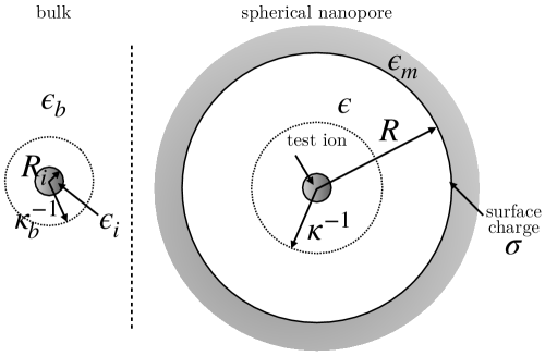
Figure 1: Sketch of the geometry: a test ion of effective radius $R_{i}$ with internal dielectric constant $\epsilon_{i}$ is transferred from the bulk (dielectric constant $\epsilon_{b}=78$, Debye-Hückel constant $\kappa_{b}$) to the center of a spherical nanopore of radius $R$ embedded in a membrane of dielectric constant $\epsilon_{m}=2$. The confined water has a lower dielectric constant than in the bulk, $\epsilon\leq\epsilon_{b}$, and due to dielectric exclusion, the Debye-Hückel screening parameter is smaller than in the bulk, i.e., $\kappa\leq\kappa_{b}$. The internal nanopore surface possibly carries a surface charge density $\sigma$.

We assume now that the nanopore is filled by an electrolyte with in general a different DH screening parameter,

$$\kappa=\sqrt{8\pi\ell_{B}\eta z^{2}\rho},$$ (30)

from the one in the bulk, where $\rho$ is the electrolyte concentration in the pore (see Fig. (1)). Moreover, we limit ourselves for the moment to the case $\sigma=0$. Generalizing the above bulk calculation to the case of an ion embedded in a spherical nanopore geometry yields a more complicated, but analytical, expression for the electrostatic potential $\Phi_{\rm p}(r)=\Phi_{i}(r)+\Delta\Phi_{\rm p}(\kappa)$ (see Appendix). (The volumetric free energy $f_{\rm p}$ obtained from the charging method leads to an integral that cannot, however, be carried out analytically.) Using $\mu^{\rm el}_{\rm p}=\frac{\beta q}{2}\Delta\Phi_{\rm p}(\kappa)$, one obtains an analytical expression for the excess electrostatic chemical potential in the pore

$$\mu^{\rm el}_{\rm p}=\frac{z^{2}\eta\ell_{B}}{2R_{i}}\left[\frac{2\kappa R_{i}}{\left(e^{2\kappa(R-R_{i})}(1+\kappa R_{i})\frac{\kappa R-1+\epsilon_{m}/\epsilon}{\kappa R+1-\epsilon_{m}/\epsilon}+1-\kappa R_{i}\right)(1+\kappa R_{i})}+\left(1-\frac{\epsilon}{\epsilon_{i}}\right)-\frac{\kappa R_{i}}{1+\kappa R_{i}}\right]$$ (31)

Taking $R\to\infty$ kills the first term in the brackets, and we recover Eq. (15) by replacing $\epsilon$ with $\epsilon_{b}$ (or $\eta=1$). We assume that the DH charging method, outlined above for the bulk case, can be carried over mutatis mutandis to the pore case to obtain $f^{\rm el}_{\rm p}$ and therefore $\omega^{\rm el}_{\rm p}$ from $\mu^{\rm el}_{\rm p}$ and $\rho$:

$$f^{\rm el}_{\rm p}=\beta\rho q\int_{0}^{1}d\xi\,\Delta\Phi_{\rm p}(\kappa\sqrt{\xi})$$ (32)

and

$$\omega^{\rm el}_{\rm p}=\frac{\epsilon_{0}\epsilon}{2q}\kappa^{2}\left(\int_{0}^{1}d\xi\,\Delta\Phi_{\rm p}(\kappa\sqrt{\xi})-\Delta\Phi_{\rm p}(\kappa)\right),$$ (33)

where we have used $2\rho\beta q^{2}=\epsilon_{0}\epsilon\kappa^{2}$. If we assume that the pore interior is in equilibrium with a bulk external reservoir, then the two electrochemical potentials are equal, $\mu_{\rm p}=\mu_{\rm b}$, where

$$\mu_{\rm p}=\ln\rho+\mu^{\rm el}_{\rm p}$$ (34)

and

$$\mu_{\rm b}=\ln\rho_{\rm b}+\mu^{\rm el}_{\rm b}.$$ (35)

Therefore the partition coefficient is $k=\rho/\rho_{\rm b}=\exp(-\Delta W_{\rm p})$, where

$$\Delta W_{\rm p}(\kappa)=\mu^{\rm el}_{\rm p}-\mu^{\rm el}_{\rm b},$$ (36)

is the difference in chemical potentials (or PMF). This PMF, which controls the transfer of an ion from the bulk to the center of the spherical nanopore, is given by

$$\Delta W_{\rm p}(\kappa) = W_{\rm conf}(\kappa,\epsilon_{m}/\epsilon)+W_{\rm DH}(\kappa)+W_{\rm Born}$$ (37)

$$= \frac{z^{2}\ell_{B}\eta\kappa}{e^{2\kappa(R-R_{i})}(1+\kappa R_{i})^{2}\frac{\kappa R-1+\epsilon_{m}/\epsilon}{\kappa R+1-\epsilon_{m}/\epsilon}+1-(\kappa R_{i})^{2}}+\frac{z^{2}\ell_{B}}{2}\left(\frac{\kappa_{b}}{1+\kappa_{b}R_{i}}-\frac{\eta\kappa}{1+\kappa R_{i}}\right)+\frac{z^{2}\ell_{B}}{2R_{i}}(\eta-1)$$ (38)

In particular, on can check that when $\kappa$ and $\kappa_{b}\to 0$, $\Delta W_{\rm p}(\kappa)$ reduces to the correct result in the absence of electrolyte, Eq. (11), comprised of the usual Born self-energy, $W_{\rm Born}$, and dielectric solvation contributions. In the case where the pore bares a surface charge density $\sigma$, one should add the following pore-charge electrostatic energy

$$\Delta W_{\rm p,\sigma}(\kappa)=\frac{\beta q\sigma\kappa}{\epsilon_{0}\epsilon}\frac{e^{\kappa(R-R_{i})}}{e^{2\kappa(R-R_{i})}(1+\kappa R_{i})(\kappa R-1+\epsilon_{m}/\epsilon)+(\kappa R+1-\epsilon_{m}/\epsilon)(1-\kappa R_{i})}$$ (39)

which leads to Eq. (12) in the limit $\kappa\to 0$.

One can, somewhat artificially, separate the excess chemical potential given in Eq. (38) into three contributions: (i) the first term $W_{\rm conf}(\kappa,\epsilon_{m}/\epsilon)$ is associated with the confinement of ions in a nanopore and depends on the ratio of dielectric constants $\epsilon_{m}/\epsilon$ and the cavity radius $R$ (note that this term increases dramatically when $R_{i}$ increases but the divergence occurs for $R_{i}>R$, i.e. an unphysical case); (ii) the second term $W_{\rm DH}(\kappa)$ is the difference in solvation energies (related to the DH chemical potential for an ion of effective radius $R_{i}$) between a hypothetic bulk with DH constant $\kappa$ and the bulk with $\kappa_{b}$; and (iii) the last term $W_{\rm Born}$ is independent of both $\kappa$ and $R$. It corresponds to the classical Born solvation energy of an ion which is transferred from the bulk to the pore with $\epsilon\neq\epsilon_{b}$ ($\eta\neq 1$). It dominates for small ion radii, and diverges for vanishing $R_{i}$ since, in this case, it corresponds to the difference of the Coulomb self-energy for point-like ions. Hence for $\epsilon<\epsilon_{b}$, the Born solvation energy impedes the entrance of ions into the nanopore.

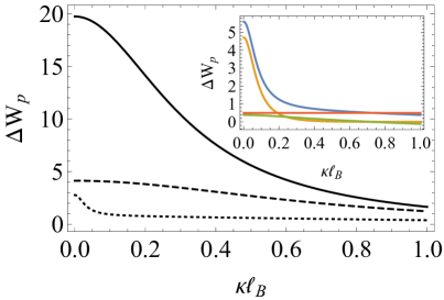
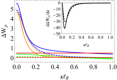
(a)                                                                             (b)

Figure 2: Potential of mean force $\Delta W_{\rm p}$ (in units of $k_{B}T$) given in Eq. (38) versus $\kappa\ell_{B}$ for $\kappa_{b}\ell_{B}=1$ (or $\rho_{b}\approx 0.19$ M), and $\epsilon=60$: (a) $R_{i}=0.3\ell_{B}$ and $R=2\ell_{B}$, $\epsilon_{m}=2$ (solid line); $R=2\ell_{B}$, $\epsilon_{m}=10$ (dashed line), $R=10\ell_{B}$, $\epsilon_{m}=2$ (dotted lines). Inset: various contributions to $\Delta W_{\rm p}$: dielectric $W_{\rm diel}$ (yellow), solvation $W_{\rm sol}$ (green), and Born $W_{\rm B}$ ones (red) for $R=4\ell_{B}$, $\epsilon_{m}=2$ with the other parameters being the same. (b) Influence of the ionic size for $\kappa_{b}\ell_{B}=1$, $\epsilon=60$, $\epsilon_{m}=2$, $R=4\ell_{B}$, and $R_{i}=0.3\ell_{B}$ (solid lines); $R_{i}=3\ell_{B}$ (dashed lines). Inset: First derivative $W^{\prime}(\kappa)$.

It is physically illuminating to define the three following contributions to the PMF

$$\Delta W_{\rm p}(\kappa)=W_{\rm diel}(\kappa,\epsilon_{m}/\epsilon)+W_{\rm sol}(\kappa)+W_{\rm Born}$$ (40)

where $W_{\rm diel}(\kappa,\epsilon_{m}/\epsilon)=W_{\rm conf}(\kappa,\epsilon_{m}/\epsilon)-W_{\rm conf}(\kappa,1)$ is the dielectric jump one, $W_{\rm sol}=W_{\rm conf}(\kappa,1)+W_{\rm DH}(\kappa)$ the solvation one, and $W_{\rm Born}$, the Born one. They depend on 6 dimensionless parameters which are $\kappa_{b}\ell_{B}$, $\kappa\ell_{B}$, $R/\ell_{B}$, $R_{i}/\ell_{B}$, $\epsilon_{m}/\epsilon_{b}$, and $\eta$. The variation of $\Delta W_{\rm p}(\kappa)$ and its different contributions with $\kappa\ell_{B}$ are shown in Fig. (2)(a) for $\kappa_{b}\ell_{B}=1$ (or $\rho_{b}\approx 0.19$ M), $\epsilon=60$, and $R_{i}=0.3\ell_{B}$ and different values of the other parameters. One clearly see that $\Delta W_{\rm p}$ decreases exponentially with $\kappa R$ and that its value at low $\kappa$ decreases with increasing $\epsilon_{m}$ or $R$, as dielectric exclusion diminishes. The inset in Fig. (2)(a) shows that the behavior of $\Delta W_{\rm p}$ is controlled by the dielectric exclusion, $W_{\rm diel}$, at small $\kappa$ and by the constant Born exclusion contribution, $W_{\rm Born}$, for $\kappa\simeq\kappa_{b}$. In any case, the solvation contribution, $W_{\rm sol}$, which accounts for the distortion of the ionic screening cloud in a confined geometry, is smaller than $k_{B}T$ and becomes slightly negative for $\kappa$ close to $\kappa_{b}$.

Finally Fig. (2)(b) shows the effect of the ionic size $R_{i}$ on $\Delta W_{\rm p}(\kappa)$ and its different contributions. For large ions ($R_{i}=3\ell_{B}$), the Born contribution decreases as expected and therefore $W\simeq W_{\rm diel}$ which remains strong for $\epsilon_{m}=2$. Interestingly, changing $R_{i}$ essentially shifts the PMF due to the change in the Born contribution, but does not modify so much its variations, and therefore its first derivative, as shown in the inset of Fig. (2)(b).

III Variational approach

In the preceding section, the charged particle at the pore center was first considered as a single ion in a dielectric cavity in the absence of electrolyte, possibly interacting with charged pore walls, leading to the solvation self-energy, $\Delta W_{\rm p}$, Eq. (11). The special case where the pore surface charge exactly counterbalances that of the ion (global electro-neutrality) corresponds to so-called strong coupling limit Netz2001 . In this case to the lowest order approximation the ion-ion interactions are neglected and only the electrostatic interactions of ions with the pore walls are taken into account.

If the ion is embedded, however, in an electrolyte-filled pore, the solvation self-energy, which depends on electrolyte concentration, is computed using a screened electrostatic potential and leads to the PMF given by Eq. (38). In this case we have assumed that $\sigma=0$ and generalized the bulk DH calculation to an electrolyte-filled pore where electro-neutrality is enforced by the ionic cloud surrounding the test charge.

In Section II, we have studied the self-energy of a single ion inside a nanopore with a given Debye constant $\kappa$. In this Section, we use this self-energy to determine self-consistently the optimized value of the Debye constant $\kappa_{v}$ using a variational approach and then use this value to obtain the optimized variational grand potential.

To study the many-body statistical physics of an electrolyte in a spherical nanopore by properly incorporating the dielectric, solvation and Born energies, we must go beyond the mean-field Poisson-Boltzmann approach and the lowest order strong coupling approach (developed in the previous section). To do so we use the Gaussian variational theoretical approach developed in Netz2003 ; PRE2010 ; PRL2010 ; JCP2011 ; JCP2016 . The full Hamiltonian is

$$\beta H=\int d\mathbf{r}\left[\frac{\varepsilon(\mathbf{r})}{2\beta e^{2}}(\vec{\nabla}\Phi(\mathbf{r}))^{2}-i\rho_{c}(\mathbf{r})\Phi(\mathbf{r})-\sum_{j=\pm}\lambda_{j}e^{z_{j}^{2}v_{i}(0)/2+iz_{j}\Phi(\mathbf{r})}\right]$$ (41)

where $\Phi(\mathbf{r})$ is a fluctuating field related to the fluctuating electric potential, $\rho_{c}(\mathbf{r})=\sigma\delta(r-R)$ is the external (volumetric) charge density that accounts for the pore surface charge density, $\sigma$ (in units of $e$), and $v_{i}(\mathbf{r})$ the bare ionic (dimensionless) Coulomb potential in a hypothetical uniform medium of dielectric constant $\epsilon_{i}$ (see Eq. (4)),

$$v_{i}(\mathbf{r},\mathbf{r}^{\prime})=\frac{\ell_{B}\epsilon_{b}}{\epsilon_{i}|\mathbf{r}-\mathbf{r}^{\prime}|}$$ (42)

[$v_{i}(0)$ is therefore the infinite bare ionic self-energy] and $\lambda_{j}$ the fugacity of ion of type $j$. This Hamiltonian is approximated by a Gaussian variational form,

$$\beta H_{0}=\frac{1}{2}\int_{\mathbf{r},\mathbf{r}^{\prime}}\left[\Phi(\mathbf{r})-i\Phi_{0}(\mathbf{r})\right]v_{0}^{-1}(\mathbf{r},\mathbf{r}^{\prime})\left[\Phi(\mathbf{r}^{\prime})-i\Phi_{0}(\mathbf{r}^{\prime})\right]$$ (43)

where $\Phi_{0}(\mathbf{r})=-i\left\langle\Phi(\mathbf{r})\right\rangle_{0}$ is the mean physical (dimensionless) variational electrostatic potential (for the variational Hamiltonian) induced by the fixed charges (e.g., the surface charge density of the walls) and $v_{0}(\mathbf{r},\mathbf{r}^{\prime})$ is the (dimensionless) electrostatic kernel governing the interaction between test ions located at $\mathbf{r}$ and $\mathbf{r}^{\prime}$. It depends directly on the dielectric distribution, but only indirectly on the surface charge $\sigma$ via $\Phi_{0}(\mathbf{r})$. Hence the two electrostatic interactions are partially decoupled via their respective sources: $\Phi_{0}(\mathbf{r})$ has as source only the fixed electrostatic charges and $v_{0}(\mathbf{r},\mathbf{r}^{\prime})$ has as source only the point test ion charges.

For sake of simplicity, we assume that in a small nanopore, $\Phi_{0}$ can be approximated by a constant Donnan potential and is therefore determined by global electro-neutrality in the pore. We first consider only point-like ions (i.e., $\epsilon_{i}=\epsilon$) and assume that the corresponding $v_{0}$ is the Green function solution to a DH equation with a constant variational DH screening parameter $\kappa_{v}$,

$$v_{0}(\mathbf{r},\mathbf{r}^{\prime};\kappa_{v})=v_{0}^{\rm DH}(\mathbf{r},\mathbf{r}^{\prime};\kappa_{v})+\delta v_{0}(\mathbf{r},\mathbf{r}^{\prime};\kappa_{v}),$$ (44)

where $\delta v_{0}(\mathbf{r},\mathbf{r}^{\prime})$ is defined as the correction to an effective bulk variational (dimensionless) DH potential in a medium with dielectric constant $\epsilon$,

$$v_{0}^{\rm DH}(\mathbf{r},\mathbf{r}^{\prime};\kappa_{v})=\eta\ell_{B}\frac{e^{-\kappa_{v}|\mathbf{r}^{\prime}-\mathbf{r}|}}{|\mathbf{r}-\mathbf{r}^{\prime}|}.$$ (45)

Clearly the correction $\delta v_{0}(\mathbf{r},\mathbf{r}^{\prime};\kappa_{v})$ takes into account the presence of dielectric inhomogeneities and therefore depends on the pore geometry. It can be evaluated exactly for cylindric JCP2011 and spherical Curtis2005 pores (see Appendix). The dielectric mismatch parameter $\eta$ has been introduced to handle the case where $\epsilon\neq\epsilon_{b}$.

For point-like ions the variational parameters $\kappa_{v}$ and $\Phi_{0}$ can then be obtained by minimizing the dimensionless volumetric variational grand-potential $\omega_{\rm v}=\beta\Omega_{\rm v}/V$ where,

$$\Omega_{\rm v}=\Omega_{0}+\left\langle H-H_{0}\right\rangle_{0},$$ (46)

and the expectation value is taken with $H_{0}$. Evaluating $\Omega_{\rm v}$ using Eq. (44) leads to JCP2011

$$\omega = -\sum_{j=\pm}\left\langle\rho_{j}(\mathbf{r})\right\rangle+\frac{\kappa_{v}^{3}}{24\pi}$$ (47)

$$+\frac{\kappa_{v}^{2}}{8\pi\ell_{B}\eta}\int_{0}^{1}d\xi\langle\delta v_{0}(\mathbf{r},\mathbf{r};\kappa_{v}\sqrt{\xi})-\delta v_{0}(\mathbf{r},\mathbf{r};\kappa_{v})\rangle+\frac{3}{R}\sigma\Phi_{0},$$

where $V=\frac{4}{3}\pi R^{3}$ is the pore volume,

$$\left\langle\rho_{\pm}(\mathbf{r})\right\rangle=\lambda_{\pm}\left\langle e^{-w_{\pm}(\mathbf{r})}\right\rangle$$ (48)

is the pore averaged concentration of cations ($+$) and anions ($-$) (the symbols $\langle\ldots\rangle$ stands for an average over the nanopore volume), which can be identified using $\rho_{\pm}=-\lambda_{\pm}\frac{\partial\omega}{\partial\lambda_{\pm}}$ and

$$w_{\pm}(\mathbf{r})=\frac{z^{2}}{2}\left[\delta v_{0}(\mathbf{r},\mathbf{r};\kappa_{v})-\eta\kappa_{v}\ell_{B}\right]\pm z\Phi_{0}$$ (49)

with

$$\lambda_{\pm}=\rho_{b}\exp({-z^{2}\kappa_{b}\ell_{B}/2})$$ (50)

the fugacity of ions of type $\pm$ (determined by the bulk reservoir with which the ions in the pore are in equilibrium). Since we have limited our approach to symmetric electrolytes with $z_{+}=z_{-}=z$, $\lambda_{+}=\lambda_{-}=\lambda$ (the generalization to asymmetric salts is straightforward but leads to more complicated equations). The two first terms on the RHS of Eq. (47) are equal to $-\beta p$, where $p=p^{\rm id}+p^{\rm el}$ is an effective pressure, composed of the ideal osmotic pressure (first term) and the electrostatic osmotic DH pressure of point ions, $-\kappa_{v}^{3}/(24\pi)$ (second term), for a hypothetical bulk with DH screening parameter equal to $\kappa_{v}$. The first (negative ideal osmotic pressure) term with a PMF $w(\mathbf{r})$ includes $\delta v_{0}(\mathbf{r},\mathbf{r})$ and $\Phi_{0}$, since the ionic concentrations are modified by the presence of the pore walls. The two last terms are surface terms, equal to $\frac{3}{R}\beta\gamma$ ($\frac{3}{R}=S/V$ for a sphere), where $\gamma$ is the surface tension, that include the dielectric ($\delta v_{0}$) and electrostatic ($\Phi_{0}$) contributions induced by the presence of the pore wall. The second bulk-like term and the third surface term in Eq. (47), which are computed using the variational DH Green function, $v_{0}=v_{0}^{\rm DH}+\delta v_{0}$, are identical to the ones obtained following the DH charging method McQuarrie :

$$\frac{\kappa_{v}^{2}}{8\pi\ell_{B}\eta}\int_{0}^{1}d\xi\langle v_{0}(\mathbf{r},\mathbf{r};\kappa_{v}\sqrt{\xi})-v_{0}(\mathbf{r},\mathbf{r};\kappa_{v})\rangle$$ (51)

In the bulk ($\delta v_{0}=\Phi_{0}=0$, $\epsilon=\epsilon_{b}$), it has been shown using this variational approach that the variational DH screening parameter $\kappa_{v}$ reduces to its usual bulk value for low enough electrolyte concentration JCP2011

$$\kappa_{b}^{2}=4\pi\ell_{B}\sum_{j=\pm}z^{2}_{j}\lambda_{j}\exp\left(\frac{z_{j}^{2}}{2}\kappa_{b}\ell_{B}\right)=4\pi\ell_{B}\sum_{j=\pm}z^{2}_{j}\rho_{j,b}$$ (52)

In the case where $R\to\infty$ and the pore is uncharged ($\delta v_{0}=\Phi_{0}=0$, $\epsilon\neq\epsilon_{b}$), the minimization of Eq. (47) leads to the following variational equation

$$\kappa_{v}^{2}=4\pi\ell_{B}\eta\sum_{j=\pm}z^{2}_{j}\lambda_{j}\exp\left(\frac{z_{j}^{2}}{2}\eta\kappa_{v}\ell_{B}\right)=4\pi\ell_{B}\eta\sum_{j=\pm}z^{2}_{j}\rho_{j}$$ (53)

which is the usual DH screening parameter for a bulk electrolyte of dielectric constant $\epsilon$.

In calculating the variational grand potential both bulk-like and surface contributions to the ionic self-energy [arising from $\delta v_{0}(\mathbf{r},\mathbf{r})$] must be accounted for in Eq. (47). Hence to take into account the ion finite size in the electrostatic self-energy, and therefore the dielectric jumps both at the pore surface and the ion surface, we have to modify $\delta v_{0}(\mathbf{r},\mathbf{r})$. In the following we modify Eq. (47) by (i) taking into account the ion finite size in the DH electrostatic potential (and free energy and chemical potential), and (ii) using the mid-point approximation Yaroshchuk2000 ; PRE2010 , i.e. computing the electrostatic self-energy only at the center of the pore, which therefore provides a lower bound for the dielectric exclusion, which is higher closer to the pore wall. We focus here on already subtle electrostatic effects and therefore do not consider the more complicated case of hard-core repulsion, which can also be included in this variational approach using a Carnahan-Starling formula for the pressure and plays a non-negligible role at high concentrations (roughly for $\rho_{b}>0.5$ mol/L) JCP2016 .

Following points (i)-(ii) listed above, the difference in chemical potentials of point-like ions in a spherical nanopore

$$\mu(\mathbf{r})-\mu_{b}=\frac{z^{2}}{2}[\delta v_{0}(\mathbf{r},\mathbf{r},\kappa_{v})+(\kappa_{b}-\eta\kappa_{v})\ell_{B}]$$ (54)

is therefore modified by taking $\mathbf{r}$ at the pore center in the average over pore volume (midpoint approximation) and replaced by the difference of chemical potentials, $\Delta W_{\rm p}(\kappa_{v})$, given in Eq. (38) to take into account the finite size of the ions. Hence $z^{2}\delta v_{0}/2$ is replaced by $W_{\rm conf}(\kappa_{v},\epsilon_{m}/\epsilon)$, and $z^{2}\ell_{B}(\kappa_{b}-\eta\kappa_{v})/2$ by $W_{\rm DH}(\kappa_{v})+W_{\rm Born}$.

The second and third terms of Eq. (47) are computed using the charging method presented in the previous section, using Eq. (25), which leads to:

$$\omega(\kappa_{v},\Phi_{0}) = -2\rho_{b}e^{-\Delta W_{\rm p}(\kappa_{v})}\cosh(z\Phi_{0})+\frac{1}{8\pi R_{i}^{3}}\left[2\kappa_{v}R_{i}-2\ln(1+\kappa_{v}R_{i})-\frac{\kappa^{2}_{v}R^{2}_{i}}{1+\kappa_{v}R_{i}}\right]$$ (55)

$$+\frac{\kappa_{v}^{2}}{4\pi z^{2}\ell_{B}\eta}\left[\int_{0}^{1}W_{\rm conf}(\sqrt{\xi}\kappa_{v})d\xi-W_{\rm conf}(\kappa_{v})\right]+\frac{3}{R}\sigma\Phi_{0}$$

As for point ions, the Born contribution enters in $\Delta W_{\rm p}$, but not the effective bulk-like pressure contribution. It is useful to write $\omega(\kappa_{v},\Phi_{0})$ entirely in terms of the difference in excess chemical potentials, $\Delta W_{\rm p}$, using $\kappa$ as the charging parameter [cf. Eq. (28)]:

$$\omega(\kappa_{v},\Phi_{0})=-2\rho_{b}e^{-\Delta W_{\rm p}(\kappa_{v})}\cosh(z\Phi_{0})+\frac{1}{2\pi z^{2}\ell_{B}\eta}\int_{0}^{\kappa_{v}}d\kappa\kappa\left[\Delta W_{\rm p}(\kappa)-\Delta W_{\rm p}(\kappa_{v})\right]+\frac{3}{R}\sigma\Phi_{0}.$$ (56)

The second term on the RHS of Eq. (56) constitutes the excess variational electrostatic grand potential, $\omega^{\rm el}(\kappa_{v})$.

Minimizing Eq. (56) with respect to the variational parameters $\Phi_{0}$ and $\kappa_{v}$ allows us to obtain the equilibrium expectations values. In the following, we focus on the ionic concentrations in the nanopore. The minimization with respect to $\kappa_{v}$ allows us to obtain immediately, owing to the mid-point approximation (cf. Eq. 1 of JCP2011 ) and the relation

$$\frac{\partial\omega^{\rm el}}{\partial\kappa_{v}}=-\frac{\kappa_{v}^{2}}{4\pi z^{2}\ell_{B}\eta}\frac{\partial\Delta W_{\rm p}}{\partial\kappa_{v}},$$ (57)

the following simple result:

$$\kappa_{v}^{2}=8\pi\ell_{B}\eta z^{2}\rho_{b}e^{-\Delta W_{\rm p}(\kappa_{v})}\cosh(z\Phi_{0})=4\pi\ell_{B}\eta z^{2}(\rho_{+}+\rho_{-}),$$ (58)

where

$$\rho_{\pm}=\rho_{b}e^{-\Delta W_{\rm p}\mp z\Phi_{0}}$$ (59)

are the concentrations in the pore and

$$k_{\pm}\equiv\frac{\rho_{\pm}}{\rho_{b}}=e^{-\Delta W_{\rm p}(\kappa_{v})\mp z\Phi_{0}}$$ (60)

the partition coefficients. The relation Eq. (57) is simply the variational analog of the usual thermodynamic identity $(\partial\omega/\partial\rho)=-2\rho(\partial\mu/\partial\rho)$ for a two component system, here a symmetric electrolyte with a total ionic concentration of $2\rho$.

The minimization with respect to the Donnan potential $\Phi_{0}$ leads to the electroneutrality condition:

$$\sigma=\frac{2}{3}zR\rho_{b}e^{-\Delta W(\kappa_{v})}\sinh(z\Phi_{0})=\frac{zR}{3}(\rho_{-}-\rho_{+})$$ (61)

Two equations similar to Eqs. (58,61), but more general, were obtained for point-like ions in a cylindrical geometry JCP2011 (without the mid-point approximation).

In particular, in the bulk limit ($R\to\infty$) for $R_{i}\neq 0$, we find the usual DH Finite Size result for the chemical potential in a solution McQuarrie , which, for $\eta\neq 1$, is generalized to include the Born contribution:

$$\mu=\ln\rho-\frac{z^{2}\eta\ell_{B}}{2R_{i}}\left[\frac{\kappa R_{i}}{1+\kappa R_{i}}+\left(1-\frac{\epsilon}{\epsilon_{i}}\right)\right].$$ (62)

IV Partition coefficients and phase diagrams

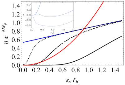
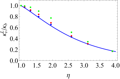
(a)                                                            (b)

Figure 3: (a) Graphical solution of the variational equation Eq. (63) for $\kappa_{b}\ell_{B}=1$, $R_{i}=0.3\ell_{B}$, $\epsilon=60$, $\epsilon_{m}=2$ and three different radii, $R/\ell_{B}=1$ (solid line), 2 (dashed line), 5 (dotted line). The black curves correspond to $\eta e^{-\Delta W_{\rm p}(\kappa_{v})}$ and the red curve to $(\kappa_{v}/\kappa_{b})^{2}$. For $R=\ell_{B}$ (respectively $R=5\ell_{B}$) the solution corresponds to the vapour (resp. liquid) phase. The case $R=2\ell_{B}$ is in the liquid phase but with a metastable vapor state. The blue curve corresponds to the asymptotic behavior $\eta e^{-W_{\rm DH}(\kappa_{v})-W_{\rm Born}}$. Inset: Associated grand-potential $\omega$, the minima of which correspond to the stable or metastable solutions. (b) Numerical solutions (symbols) corresponding to the intersection between the red and blue curves in (a) versus $\eta=\epsilon_{b}/\epsilon$ for $\kappa_{b}\ell_{B}=0.5$ (blue), 1 (red) and 2 (green). The curve corresponds to the approximate solution given in Eq. (64).

We first focus on the case where the pore surface is neutral $\sigma=0$ (and therefore, according to Eq. (61), $\Phi_{0}=0$, because we are considering only symmetric electrolytes). The partition coefficient is the same for coions and counterions, $k=e^{-\Delta W_{\rm p}(\kappa_{v})}$. By minimizing the grand-potential $\omega(\kappa_{v})$, we find one stable physical solution (ionic fluid phase) or two physical (vapor and liquid) solutions for $\kappa_{v}$ (stable or metastable) [and one unstable (unphysical) solution], corresponding to a first order phase transition, depending on the values of $\rho_{b}$ (or equivalently $\kappa_{b}^{2}$) and $R$. The variational equation Eq. (58) can be rewritten

$$\frac{\kappa_{v}^{2}}{\kappa_{b}^{2}}=\eta e^{-\Delta W_{\rm p}(\kappa_{v})}.$$ (63)

When there are three solutions, the (stable or metastable) solution where $\kappa_{v}\gtrsim 0$ corresponds to an ionic vapor phase with almost no ions entering the nanopore. The second (stable or metastable) solution is obtained for $\kappa_{v}\simeq\kappa_{b}$ and corresponds to an ionic liquid phase. The solution in between corresponds to a maximum of $\omega(\kappa_{v})$ and is therefore unstable. The graphical determination of the solutions is illustrated in Fig. (3)(a) for $\kappa_{b}\ell_{B}=1$, $R_{i}=0.3\ell_{B}$, $\epsilon=60$, $\epsilon_{m}=2$ and three different radii, $R/\ell_{B}=1,2,5$. The transition occurs as soon as the value of $\Delta W_{\rm p}$ is large at small $\kappa$ and its variations are abrupt enough, i.e. when the dielectric contribution $W_{\rm diel}$ is large enough.

Although it is impossible to obtain an analytical expression for the solutions of Eq. (63), one can give a simple estimate in the limit of large pore radius $R$ for which $W_{\rm conf}$ is negligible. Indeed, in this limit the solution for the ionic liquid phase (at large $\kappa_{v}$) is essentially controlled by the Born and to a lesser extent DH contributions to the PMF. Graphically it corresponds to the intersection between the blue and red curves in Fig. (3)(a). Hence an analytical estimate of the solution in the liquid state, a priori valid at large $R$, is obtained by neglecting both the confinement and DH contributions in the PMF Eq. (38), leading to

$$\kappa_{v}^{\rm L}\approx\kappa_{b}\sqrt{\eta}e^{-W_{\rm Born}/2}=\kappa_{b}\sqrt{\eta}\exp\left[-\frac{z^{2}\ell_{B}}{4R_{i}}(\eta-1)\right]$$ (64)

One can check in Fig. (3)(b) that this expression is in good agreement with the numerical solutions obtained by neglecting $W_{\rm conf}$ in Eq. (63). It is slightly less good for large $\kappa_{b}$ since the DH contribution to the PMF becomes more important. In particular, one notices that $\kappa_{v}^{\rm L}$ decreases when $\eta$ increases, since the Born effect, $e^{-W_{\rm Born}/2}$, overwhelms the factor $\sqrt{\eta}$ coming from the increase of the Bjerrum length.

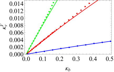
Figure 4: Numerical solutions (symbols) of the variational equation Eq. (63) in the ionic vapor phase versus $\kappa_{b}$ for $R/\ell_{B}=2$ (blue), 3 (red) and 4 (green) ($R_{i}=0.3\ell_{B}$, $\epsilon=60$ and $\epsilon_{m}=2$). The curves corresponds to the approximate solution given in Eq. (65).

Knowing that the ionic vapor phase is obtained for low values of $\kappa_{v}$, a good and simple estimate of the solution to Eq. (63) in this phase, $\kappa_{v}^{\rm V}$, is obtained by taking the limit $\kappa_{v}\to 0$ on the rhs. of Eq. (63). This approximation allows one to make a connection between this limit of the variational approach and the salt-free pore result previously obtained in Section II (Eq. 11). One then has

$$\kappa_{v}^{\rm V}\approx\kappa_{b}\sqrt{\eta}e^{-\Delta W_{\rm p}(0)/2}$$ (65)

where

$$\Delta W_{\rm p}(0)=\frac{z^{2}\ell_{B}}{2}\left(\frac{\epsilon_{b}/\epsilon_{m}-\eta}{R}+\frac{\eta-1}{R_{i}}+\frac{\kappa_{b}}{1+\kappa_{b}R_{i}}\right)$$ (66)

which are, respectively, the dielectric and Born contributions for an empty pore (see Eq. (11)) minus the classical DH chemical potential in the bulk. We compare this result with the numerical solution in Fig. (4). The agreement is extremely good at low $\kappa_{b}$. One could in principle improve the approximate solution Eq. (65) by expanding $\Delta W_{\rm p}(\kappa_{v})$ to order 2 in $\kappa_{v}$, but this leads to a much complicated expression. Interestingly, one notices that the ratio between $\kappa_{v}^{\rm V}$ and $\kappa_{v}^{\rm L}$ is essentially controlled by the first dielectric contribution of Eq. (66), i.e. the nanopore radius $R$ and the dielectric jump $\epsilon_{m}^{-1}-\epsilon^{-1}$.

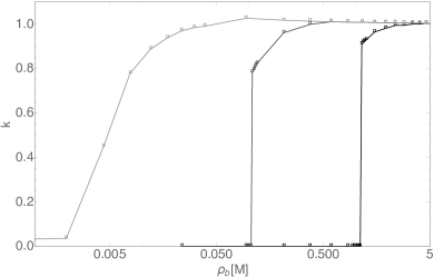
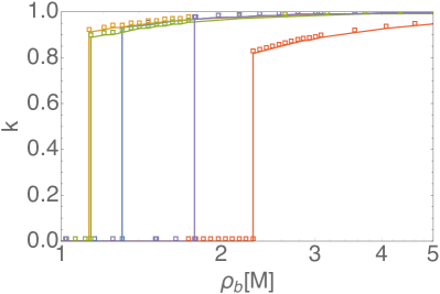
(a)                                                                         (b)

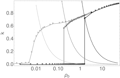
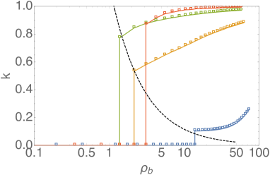
(c)                                                                         (d)

Figure 5: (a) Ionic partition coefficient $k=\rho/\rho_{b}=\kappa_{v}^{2}/(\eta\kappa_{b}^{2})$ vs the bulk concentration $\rho_{b}$ (log-linear plot) for various neutral pore radii ($R/\ell_{B}=1,2,5$ from right to left), $\epsilon=\epsilon_{b}=78$ and $\epsilon_{m}=2$. The transition from the ionic vapor phase ($k\simeq 0$) and the ionic liquid phase ($k\simeq 1$) occurs for small radii and disappears for larger pores. The effective ionic radius has been fixed at $R_{i}=0.3\ell_{B}$. (b) Same figure for different values of the effective ionic radius $R_{i}/\ell_{B}=0$ (purple), 0.1 (blue), 0.2 (orange), 0.4 (green), 0.8 (red) ($R=\ell_{B}$ and $\epsilon=\epsilon_{b}$). (c) Same as (a) for $\epsilon=60$ ($\eta=1.3$) (corresponding to Fig. (3)). One clearly observes the effect of the Born self-energy that increases the critical $\rho_{b}$ and decreases the limiting value of $k$ in the liquid state. (d) Same as (b) for $\epsilon=60$ ($\eta=1.3$) and $R_{i}/\ell_{B}=0.1$ (blue), 0.2 (orange), 0.4 (green), 0.8 (red). The dashed lines correspond to the case of a single ion on average in the pore.

The partition coefficient $k$ is shown in Fig. (5)a for nanopore radius $R=1,2$ and $5\ell_{B}$ and $\eta=1$ (without Born exclusion). For the smallest radii a discontinuous increase of $k$ occurs at coexistence values of the bulk concentration: for $R=\ell_{B}$ the coexistence value is $\rho_{b}^{\rm coex}\simeq 1.2$ M and for $R=2\ell_{B}$, it decreases to $\rho_{b}^{\rm coex}\simeq 0.11$ M. This discontinuous transition disappears when $R=5\ell_{B}$, leading to a smooth increase of $k(\rho_{b})$ with $\rho_{b}$. This transition has already been predicted theoretically without Born exclusion for point-like PRL2010 ; JCP2011 and finite-sized ions JCP2016 in cylinders. As already noticed in PRE2010 the mid-point approximation used here leads to larger values of $\rho$ in the bulk phase close to $\rho_{b}$, whereas excluded volume interactions must be properly included to obtain $\rho\simeq\rho_{b}$ without this approximation, as shown in JCP2016 .

To illustrate the role of the finite ionic size in $W_{\rm diel}$ and $W_{\rm sol}$, we present in Fig. (5)b the variation of $k(\rho_{b})$ for various ionic radii and $\eta=1$: $R_{i}=0$ (point-like ions), 0.1, 0.2, 0.4 and $0.8\ell_{B}$ for $R=\ell_{B}$. In all cases, one still observes the discontinuous transition but the variation of the coexistence bulk concentration, $\rho_{b}^{\rm coex}$, with $R_{i}$ is non-monotonous: it first decreases slightly when $R_{i}$ increases up to $R_{i}=0.2\ell_{B}$ and then increases, reaching a larger value than for point-like ions for $R_{i}=0.8\ell_{B}$. This is directly related to the variation of the dielectric contribution to the PMF, $W_{\rm diel}$, which is also non-monotonous [see Fig. (2)], decreasing when $R_{i}$ increases up to approximatively $R_{i}\sim R/2$ and then increasing again due to the term in $\exp[2\kappa(R_{i}-R)]$ in the first term of $W$ in Eq. (38).

The role of the Born self-energy in the PMF, $W_{\rm Born}$, is highlighted in Fig. (5)(c) for $\eta\neq 1$ and in Fig. (5) (d) for various values of $R_{i}$. The partition coefficients shown in these two figures have a lower saturation value, controlled by $\exp(-W_{\rm Born})$ which is independent of $\kappa_{v}$. Hence, even in the liquid state, the Born solvation energy decreases the concentration in the pore. This is a direct consequence of the result that the Born contribution dominates the PMF in the liquid state (see Fig. (2)). Moreover the transition is shifted to higher bulk critical values, especially for small ions, due to the factor $1/R_{i}$ in $W_{\rm Born}$. The dashed lines correspond to the case of a single ion in the pore on average, fixed by $k=(\frac{4}{3}\pi R^{3}\rho_{b})^{-1}$. One clearly see that it crosses the transition for all $R$ [Fig. (5)(c)] and $R_{i}$ [Fig. (5)(d)]. Hence the vapor state corresponds to less than one ion in the pore on average. As in Fig. (5)(b), Fig. (5)(d) shows a non-monotonous variation of the critical bulk concentration with $R_{i}$.

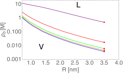
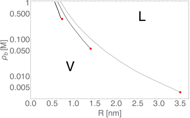
(a)                                                                         (b)

Figure 6: (a) Phase diagram (linear-log plot) in the pore radius $R$ vs. bulk concentration $\rho_{b}$ plane for 3 different nanopore dielectric constants ($\epsilon=20,40,60,70,78$ from top to bottom) for $R_{i}=0.3\ell_{B}$ and $\epsilon_{m}=2$. The left bottom (respectively right top) corner corresponds to the ionic vapor (resp. liquid) phase, and the critical point $(R^{*},\rho_{b}^{*})$ is shown in red. (b) Same figure as in (a) but for $\epsilon_{m}=2,5,10$ from right to left ($\epsilon=60$ and $R_{i}=0.1\ell_{B}$, linear-log plot).

By plotting this coexistence concentration $\rho_{b}^{\rm coex}$ corresponding to the first order transition as a function of the nanopore radius, we can construct the phase diagram shown in Fig. (6)(a) for four different values of the confined water dielectric constant, $\epsilon$, and fixed membrane one, $\epsilon_{m}=2$. For large $\rho_{b}$ and $R$ the nanopore is in the ionic liquid state, and below the coexistence curve, for low $\rho_{b}$ and $R$ it is in the ionic vapor one. Clearly the coexistence line moves to higher $\rho_{b}$ values when $\epsilon$ decreases (i.e. $\eta$ increases). Indeed, the dielectric contribution to the PMF $W_{\rm diel}$ is proportional to $\eta$ for fixed $\kappa_{v}$, which thus favors the ionic vapor state. Interestingly, the critical radius $R^{*}$ (in red) does not change with $\epsilon$. This is probably due to the result that the critical point is fixed by the abrupt decrease of $\Delta W_{\rm p}(\kappa_{v})$, which is almost independent of the Born self-energy [as shown in the inset of Fig. (2)(b)].

In Fig. (6)(b) we illustrate the role of the membrane dielectric constant $\epsilon_{m}$, by changing its value from 2 to 10 for a fixed $\epsilon=60$. Increasing $\epsilon_{m}$ moves the coexistence line to the left and favors the liquid state, but the critical point also moves to lower radii $R^{*}$ and larger critical bulk concentrations $\rho_{b}^{*}$.

We illustrate the influence of the ion radius $R_{i}$ in Fig. (7) using $R_{i}=0,0.1,0.2,0.5$ and $0.8\ell_{B}$ for (a) $\epsilon=\epsilon_{b}$ and (b) $\epsilon=60$. The fact that the curves are almost superimposed in case (a) confirms that $R_{i}$ plays an essential role only in the Born exclusion (last term on the RHS of Eq. (38)). Indeed the terms that depend on $\kappa R_{i}\ll 1$ do not influence much $W_{\rm diel}$ and $W_{\rm sol}$. On the contrary, for $\eta>1$, Fig. (7) shows that the liquid state is favored when $R_{i}$ increases, owing to the decrease in $1/R_{i}$ in $W_{\rm Born}$, leading to a decrease in Born exclusion. The non-monotonous behavior observed in Fig. (5)(d) (for $R=\ell_{B}=0.7$ nm) occurs only for small nanopore radius $R$. In any case the shift of the coexistence curve remains small.

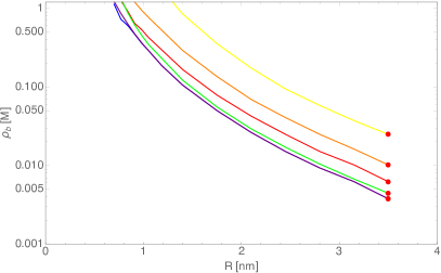
Figure 7: Same as Fig. 6 for three different ion radii ($\epsilon_{m}=2$): for $\epsilon=78$ the three curves are almost superimposed [$R_{i}/\ell_{B}=0$ (light blue), 0.2 (blue), and 0.5 (purple)], whereas they are shifted to larger $\rho_{b}$ values when $R_{i}$ decreases for $\epsilon=60$ [$R_{i}/\ell_{B}=0.1$ (yellow), 0.2 (orange), 0.5 (red), and 0.8 (green)].

We study the influence of the pore radius $R$ on the partition coefficient $k$ and the total osmotic pressure in the pore $p=-k_{B}T\omega$ by inserting $\kappa_{v}$ after minimization for $\rho_{b}=0.5$ mol/L (see Fig. (8)). Similarly to Fig. (5)(a) and (c), $k$ abruptly increases from the ionic vapor state at low radius to the liquid one for large radius with a critical radius of $R\simeq 0.9$ nm for $\eta=1$, $\simeq 1$ nm for $\eta=1.3$ ($\epsilon=60$) and $\simeq 1.2$ nm for $\eta=1.95$ ($\epsilon=40$). The saturation value for $k$ is quickly reached and decreases from 1 to 0.4 when $\eta$ increases. It corresponds to the decrease of $\kappa_{v}^{L}$ given in Eq. (64) since $k\approx(\kappa_{v}^{L})^{2}/(\eta\kappa_{b}^{2})=e^{-W_{\rm Born}}$. Hence, in the liquid state and at fixed $R$, the concentration in the pore $\rho$ decreases when $\eta=\epsilon_{b}/\epsilon$ increases. The signature of the transition also appears in Fig. (8)(b) where the pressure increases by 3 orders of magnitude at the transition for $\eta=1$. When $\eta$ increases the transition occurs at larger radius and the jump is smaller, of one order of magnitude for $\epsilon=20$.

In the liquid state and for large $\rho_{b}$ or large $R$, the pressure is given by the grand-potential, $\beta p=-\omega(\kappa_{v}^{L})$, by assuming that the pore term (which depends on $W_{\rm conf}$) is negligible. In this limit the pressure can therefore be approximated by the usual bulk DH result (see, e.g., McQuarrie ), but with a salt concentration and dielectric constant appropriate for a nanopore and in general different from the real bulk values:

$$\beta p_{b}=2\rho_{b}\ e^{-W_{\rm Born}}-\frac{1}{8\pi R_{i}^{3}}\left[2\kappa_{v}^{L}R_{i}-2\ln\left(1+\kappa_{v}^{L}R_{i}\right)-\frac{(\kappa_{v}^{L}R_{i})^{2}}{1+\kappa_{v}^{L}R_{i}}\right],$$ (67)

with $\kappa_{v}$ approximated by $\kappa_{v}^{L}$, given in Eq. (64), which is a very accurate for large $R$. This equivalent bulk pressure decreases when $\eta$ increases essentially due to the first ideal term, since the concentration in the pore $\rho$ decreases when $\eta$ increases. It is roughly $0.18k_{B}T/\ell_{B}^{3}\simeq 20$ bar (respectively $0.06k_{B}T/\ell_{B}^{3}$) for $R_{i}=0.3\ell_{B}$, $\rho_{b}=0.5$ mol/L and $\eta=1$ (resp. $\eta=1.95$). It indeed corresponds to the limiting values for large $R$ of the black and light grey curves respectively observed in Fig. (8)b. Hence the pressure is a good observable to study the ionic LV transition and the influence of $\eta$ on the critical radius.

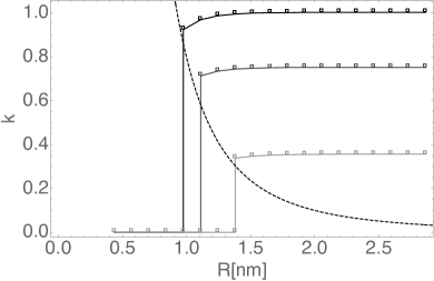
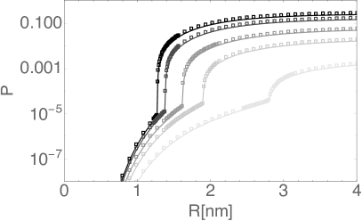
(a)                                                                         (b)

Figure 8: Influence of the pore radius $R$ (for $\rho_{b}=0.5$ mol/L, $R_{i}=0.3\ell_{B}$) on (a)  the partition coefficient $k$ (the dashed line corresponds to the case of a single ion on average in the pore) for $\epsilon=\epsilon_{b},60,40$ from left to right. (b) Total osmotic pressure $p=-k_{B}T\omega$ (in units of $k_{B}T/\ell_{B}^{3}\simeq 1.1\times 10^{7}$ Pa at room temperature) versus $R$ for $\epsilon=\epsilon_{b},60,40,30,20$ from left to right.

Finally, we consider the case of a slightly charged pore with $\sigma=-0.02$ C/m². We plot in Fig. (9) the partition coefficient of counterions $k_{+}(\rho_{b})$ and co-ions $k_{-}(\rho_{b})$ for $R/\ell_{B}=1,2$, and 5 and for $\epsilon=78$ and 60. As expected for this surface charge polarity, $k_{+}>1$ and $k_{-}<1$. Moreover, the transition remains visible on $k_{-}$, but not on $k_{+}$. Finally, as also expected, the decrease of $\epsilon$ from $\epsilon_{b}$ to 60 decreases both $k_{+}$ and $k_{-}$ in the liquid phase, due to Born exclusion. For low $\rho_{b}$, $k_{-}\simeq 0$ and following Eq. (61), one has $k_{+}\simeq 3|\sigma|/(eR\rho_{b})$ which corresponds to the asymptotic lines at low $\rho_{b}$ observed in Fig. (9).

For a small pore radius, $R=\ell_{B}$, and a lower value of surface charge density, $\sigma=-0.002$ C/m², which could be due for instance to a (partial) charge defect on the nanopore surface, the transition is also noticeable on $k_{+}$ at almost the same bulk density as for $\sigma=-0.02$ C/m², $\rho_{b}^{\rm coex}\simeq 0.025$ M (respectively 0.03 M) for $\eta=1$ (resp. $\eta=1.3$). This is because at this $\rho_{b}$, one has $k_{+}=3|\sigma|/(R\rho_{b})\simeq 0.35<1$, and a jump occurs at the transition to a value larger than 1. Hence, for low enough surface charge $|\sigma|$ and low nanopore radius $R$, the transition is still noticeable on the counter-ions partition coefficient. For larger $|\sigma|$ the system remains in the Good Co-ion Exclusion (GCE) regime, where $k_{-}\ll k_{+}$, for a wide range of reservoir concentration values $\rho_{b}$.

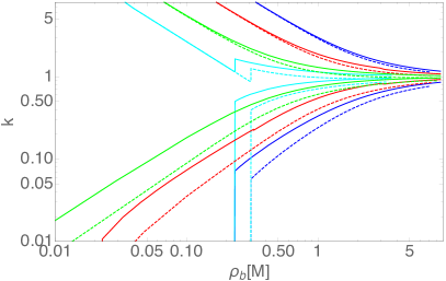
Figure 9: Partition coefficient of counterions $k_{+}(\rho_{b})$ (top) and co-ions $k_{-}(\rho_{b})$ (bottom) for various pore radii with $\epsilon=78$ (solid lines) and $\epsilon=60$ (dashed lines) for a charged nanopore with $\sigma=-0.02$ C/m² ($R_{i}=0.3\ell_{B}$): $R=\ell_{B}$ (blue), $R=2\ell_{B}$ (red), and $R=5\ell_{B}$ (green). The transition is also visible on $k_{+}$ for a smaller surface charge $\sigma=-0.002$ C/m² (cyan).

V Discussion and concluding remarks

In this article, we have studied the statistical physics of an electrolyte in a spherical nanopore of radius in the nanometer range in contact with a bulk reservoir. We focused on the influence of the dielectric constant of the water confined inside the pore $\epsilon_{m}\leq\epsilon\leq\epsilon_{b}$ and the Born ionic radius $R_{i}$ (roughly equal to to the hard-core ion plus water radius) on the partition coefficient and the osmotic pressure. To do so we first computed the PMF for a test ion located at the center of the pore, given in Eq. (38), and then determined variationally the Debye screening parameter $\kappa_{v}$ inside the pore by minimizing the variational grand-potential $\omega$ given in Eq. (55). The partition coefficient inside the pore is governed by the three intertwined contributions to the PMF that take into account ionic correlations: the dielectric contribution, $W_{\rm diel}$, which is the only one that depends on the dielectric jump at the nanopore surface ($\epsilon_{m}^{-1}-\epsilon^{-1}$), the solvation one, $W_{\rm sol}$, and the Born self-energy, $W_{\rm Born}$, which depends on the dielectric mismatch between the pore and the bulk ($\epsilon^{-1}-\epsilon_{b}^{-1}$), but does not depend explicitly on $\kappa_{v}$ and is therefore independent of the ionic concentration in the pore.

For $\epsilon_{m}=2$, the first order transition between a ionic vapor state (found for low bulk concentration $\rho_{b}$ and small pore radius $R$) to a liquid state (for larger $\rho_{b}$ and $R$), is induced by dielectric exclusion and has already been studied for point-like ions (and finite sized ones without Born exclusion). Thanks to the determination of the variational grand-potential integrating Born exclusion, we are able to construct the phase diagram and the coexistence curves in the plane ($R,\rho_{b}$) for this more general previously unstudied case. We show that this transition survives for $20\leq\epsilon\leq\epsilon_{b}=78$ for ions of Born radius $R_{i}=0.3\ell_{B}\simeq 0.2$ nm. For lower $\epsilon$ values, the pore remains in the vapor state, with no ions entering the pore over the whole accessible range of $\rho_{b}$. We have shown how the Born self-energy decreases by a factor $\simeq\exp(-W_{\rm Born})$ the value of the partition coefficient $k=\rho/\rho_{b}$ in the liquid state. Moreover the critical radius $R^{*}$ does not change with $\epsilon$ (whereas $\rho_{b}^{*}$ increases when $\epsilon$ decreases) and its value is fixed by $\epsilon_{m}$. Finally we suggest that it would be insightful to study experimentally the influence of the low water confined dielectric constant by varying the pore radius $R$. In particular the transition studied here has a clear signature on the osmotic pressure inside the pore. For charged pores, the system remains in the Good Co-ion Exclusion (GCE) regime, where $k_{-}\ll k_{+}$, for a wide range of reservoir concentrations, $\rho_{b}$.

The application of our method presented in detail here can be applied to blue energy production using carbon nanotubes and other nanoporous systems where the external medium (membrane) has a lower dielectric constant than that of the confined electrolyte solution. In principle our approach can also be extended to the opposite case where the membrane has a larger dielectric constant than the confined solution. Ions are then attracted towards the pore surface due to dielectric effects. This is for instance the case for the carbon electrodes used to harvest blue energy. It is then essential to include properly in the theory the excluded volume interactions to avoid any unphysical increase of the ionic concentration near the pore surface. One way to do so would be to use the approach developed in JCP2016 .

Although the ions are assumed to be in equilibrium in this study, it is well known that, in the linear response framework, the partition coefficients $k_{\pm}$ can be plugged into the electrokinetic coefficients to study electrokinetic transport in long nano-channels Schoch ; Yaroshchuk2000 ; revue_John ; PRE . Within this framework we intend in the future to study the role of the confined water dielectric constant on the experimentally measurable transport coefficients. An important question for ionic transport concerns the influence of dielectric mismatch on ion mobility, a topic already studied via simulations Erik . Especially important industrial applications include membrane nanofiltration Yaroshchuk2000 ; revue_John ; Sym2007 ; Sym2009 and blue energy production using osmotic pressure gradients Bocquet_charlaix . The potential role and importance of ionic liquid-vapor phase transitions in these applications remain to be determined.

Several approximations have been adopted in this study. The main one concerns the mid-point approximation, which consists in assuming that the PMF of an ion located anywhere in the nanopore is equal to the one computed for an ion located at the pore center. The PMF for a point-like ion is given in the Appendix and shows increasing dielectric repulsion close to the pore wall. This effect, which forces the ions to be located close to the center, can and should be studied by numerical simulations. The second approximation is that we did not consider explicitly the hard core excluded volume interaction, the finite radius of the ions entering only in the electrostatic contribution to the PMF. We have shown in JCP2016 that for cylindrical pores and without the mid-point approximation this excluded volume interaction increases the partition coefficient $k$ in the liquid phase roughly by a factor of 2, such that it saturates to 1 for $\rho_{b}>2$ M. Since in this study we observe the expected saturation to 1, one can suppose that there is a kind of beneficial compensation between these two approximations. Moreover, we have assumed, in the case of a charged pore, and following our previous studies PRE2010 ; PRL2010 ; JCP2011 ; JCP2016 , that electroneutrality is satisfied following Eq. (61) and that the surface charge does not appear explicitly in the self-energy $\Delta W_{\rm p}$. This issue, which has been questioned recently by Levy et al. Levy_Bazant remains to be clarified for instance by Monte Carlo simulations. It would also be extremely interesting to study the ionic LV transition for the mesoscopic model proposed here using appropriate simulation techniques.

An open question in the theory of electrolytes concerns the relationship between the field theoretical variational method adopted here and the Splitting Field method Lue2015 developed previously to study in an approximate way the subtle crossover between the mean-field Poisson-Boltzmann and strong-coupling limits. We have tried here to shed some (faint) light on this question and plan in the future to use the simplified setting of a spherical pore to further elucidate it.

Finally, our results are obtained within the hypothesis of continuous and homogeneous media. As already explained in the introduction the profile of the dielectric constant is not uniform in the nanopore, increasing from the surface to the center Bonthuis2012 ; Loche . This recent numerical work means that ions will be further excluded from the region close to the pore surface and forced to be located at the center. This effect can be reinterpreted in our model as a reduction of the effective pore radius. Hence the coexistence lines in the phase diagrams in the pore radius vs. bulk concentration plane (see Figs. 6,7) would be slightly shifted to the right (towards higher bulk concentrations). Furthermore, taking into account the ionic excluded volume in the grand-potential leads to a shift of the coexistence line towards smaller bulk concentrations because, as shown in JCP2016 , this interaction strongly modifies the PMF in the bulk.

Furthermore to properly model the dielectric constant the solvent molecules should be modeled as self-orienting dipoles, which makes it depend in principle also on the salt concentration. This has been studied in the bulk using field-theoretic approaches Koehl ; Levy ; Adar . Developing these types of approaches to the case of a confined electrolyte would be an interesting objective for future work.

Extending our work to the case of discrete fixed charges would be an important but challenging future endeavor. The influence of such dopant charges located along the pore has been studied in simple one-dimensional nanopores by assuming a 1D Coulomb potential between charges (meaning that the electric field does not enter the membrane at all, see Zhang2 ). These discrete fixed charges can induce interesting and surprising effects phenomena, such as ion exchange phase transitions Zhang2 or the fractional Wien effect  Kavokine2 . Because of the complexity of the problem the case of discrete charges with a tunable dielectric constant inside the pore would, however, most likely require numerical simulation techniques.

Appendix

In this appendix, we give the electrostatic potential of the studied system, composed of a charged ion (charge $q$, radius $R_{i}$, dielectric constant $\epsilon_{i}$) located at the center of a spherical nanopore of radius $R$. The inside of the pore is filled by an electrolyte of dielectric constant $\epsilon$ and Debye screening parameter $\kappa$ and the outside of the pore is composed of a dielectric medium of dielectric constant $\epsilon_{m}$ devoid of electrolyte. For this system the electrostatic potential, $\Phi(r)$, is given, respectively within the ion, inside the pore, and outside the pore, by

$$\Phi_{i}(r) = \frac{q}{4\pi\epsilon_{0}\epsilon_{1}}\left[\frac{1}{r}-\frac{1}{R_{i}}+\frac{\epsilon_{1}}{\epsilon R_{i}}\frac{2\kappa R_{i}\sigma e^{\kappa(R-R_{i})}+\kappa R+1-\epsilon_{m}/\epsilon+e^{2\kappa(R-R_{i})}(\kappa R-1+\epsilon_{m}/\epsilon)}{e^{2\kappa(R-R_{i})}(\kappa R_{i}+1)(\kappa R-1+\epsilon_{m}/\epsilon)-(\kappa R_{i}-1)(\kappa R+1-\epsilon_{m}/\epsilon)}\right]$$ (68)

$$\Phi(r) = \frac{q}{4\pi\epsilon_{0}\epsilon r}\frac{e^{\kappa(R-r)}\left[e^{\kappa(R-R_{i})}(\kappa R-1+\epsilon_{m}/\epsilon)+\sigma(\kappa R_{i}-1)\right]+e^{\kappa(r-R_{i})}\left[\kappa R+1-\epsilon_{m}/\epsilon+\sigma(\kappa R_{i}+1)e^{\kappa(R-R_{i})}\right]}{e^{2\kappa(R-R_{i})}(\kappa R_{i}+1)(\kappa R-1+\epsilon_{m}/\epsilon)-(\kappa R_{i}-1)(\kappa R+1-\epsilon_{m}/\epsilon)}$$ (69)

$$\Phi_{m}(r) = \frac{q}{4\pi\epsilon_{0}\epsilon r}\frac{\sigma\left[\kappa R_{i}-1+e^{2\kappa(R-R_{i})}(1+\kappa R_{i})\right]+2\kappa Re^{\kappa(R-R_{i})}}{e^{2\kappa(R-R_{i})}(\kappa R_{i}+1)(\kappa R-1+\epsilon_{m}/\epsilon)-(\kappa R_{i}-1)(\kappa R+1-\epsilon_{m}/\epsilon)}.$$ (70)

For the general case of finite size ions the link between $\Phi(r)$ (Section II) and $v_{0}(\mathbf{r},\mathbf{r}^{\prime};\kappa_{v})$ (Section III) is

$$z^{2}v_{0}(\mathbf{r},\mathbf{0};\kappa_{v})=\beta q\Phi(r).$$ (71)

The dimensionless electrostatic Green function (or potential) governing the interaction between an elementary point charge located at point $\mathbf{r}^{\prime}$ and another one at point $\mathbf{r}$ (such that $|\mathbf{r}^{\prime}|<|\mathbf{r}|$) in a neutral spherical pore can be computed exactly for point-like ions Curtis2005 and is given (in units of $k_{B}T$) by

$$v_{0}(\mathbf{r},\mathbf{r}^{\prime})=\sum_{l,m}V_{l}(r,r^{\prime})Y_{lm}(\theta,\phi)Y_{lm}^{*}(\theta^{\prime},\phi^{\prime})$$ (72)

where $Y_{lm}$ are the spherical harmonics and

$$V_{l}(r,r^{\prime})=4\pi\kappa\ell_{B}\frac{\epsilon_{b}}{\epsilon}i^{\prime}_{l}(\kappa r^{\prime})\left[k_{l}(\kappa r)-\frac{\kappa R\ k^{\prime}_{l}(\kappa R)+\frac{\epsilon_{m}}{\epsilon}k_{l}(\kappa R)}{\kappa R\ i^{\prime}_{l}(\kappa R)+\frac{\epsilon_{m}}{\epsilon}i_{l}(\kappa R)}i_{l}(\kappa r)\right]$$ (73)

with $i_{l}(x)=\sqrt{\pi/(2x)}I_{l+1/2}(x)$, $k_{l}(x)=\sqrt{2x/\pi}K_{l+1/2}(x)$ where $I_{l}$ and $K_{l}$ are the modified Bessel functions of the first and second kinds, respectively, and $i^{\prime}(x)$ and $k^{\prime}(x)$ are their derivatives.

The case $l=0$ corresponds to an ion located at the center of the spherical nanopore for which the potential, $v_{0}(r,0)$, is isotropic and $\mathbf{r}^{\prime}=0$. Using $k_{0}(x)=e^{-x}/x$ and $i_{0}(x)=\sinh(x)/x$, $v_{0}(r,0)$ simplifies to

$$v_{0}(r,0)=\ell_{B}\frac{\epsilon_{b}}{\epsilon}\frac{e^{-\kappa r}}{r}+2\ell_{B}\frac{\epsilon_{b}}{\epsilon}D(\epsilon_{m}/\epsilon,\kappa R)\frac{\sinh(\kappa r)}{r}$$ (74)

where

$$D(a,x)=\frac{x+1-a}{e^{2x}(x-1+a)+x+1-a}$$ (75)

Hence we recover $z^{2}v_{0}(r,0)=\beta q\lim_{R_{i}\to 0}\Phi(r)$ for point like ions and $\sigma=0$.

From Eq. (74) on obtains directly for point like ions

$$\mu-\mu_{b} = \frac{z^{2}}{2}\lim_{r\to 0}[v_{0}(r,0)-v_{c}(r)]+\frac{z^{2}\kappa_{b}\ell_{B}}{2}$$ (76)

$$= \frac{z^{2}\ell_{B}}{2}\left[\frac{\epsilon_{b}}{\epsilon}2\kappa D(\epsilon_{m}/\epsilon,\kappa R)+\kappa_{b}-\frac{\epsilon_{b}}{\epsilon}\kappa+\left(\frac{\epsilon_{b}}{\epsilon}-1\right)\lim_{r\to 0}\frac{1}{r}\right]$$ (77)

where we identify the three contributions for point-like ions corresponding to those of $\Delta W_{\rm p}(\kappa)$ given in Eq. (38) for finite size ones. The final term (Born self-energy) for point-like ions formally diverges when $\epsilon\neq\epsilon_{b}$, which shows the crucial importance of taking into account the finite ion size in this case. For $\epsilon=\epsilon_{m}$ (no dielectric jump), the first term in the brackets simplifies to $\frac{\epsilon_{b}}{\epsilon}\kappa[1-\tanh(\kappa R)]$ (confinement solvation term) and vanishes for $R\to\infty$.

References

- (1) R. Schoch, J. Han, and P. Renaud, Transport phenomena in nanofluidics, Rev. Mod. Phys. 80, 839-883 (2008).
- (2) H. Chmiel, X.Lefebvre, V. Mavrov, M. Noronha, J. Palmeri, Computer Simulation of Nanofiltration, Membranes and Processes, in: Handbook of Theoretical and Computational Nanotechnology, edited by Michael Rieth and Wolfram Schommers, Volume 5, Pages 93-214, American Scientific Publishers, 2006.
- (3) Y. Levin, Electrostatic correlations: from plasma to biology, Rep. Prog. Phys. 65, 1577 (2002).
- (4) L. Bocquet, and E. Charlaix, Nano uidics, from bulk to interfaces, Chem. Soc. Rev. 39, 1073-1095 (2010).
- (5) A. Szymczyk, N. Fatin-Rouge, P. Fievet, C. Ramseyer and A. Vidonne, Identification of dielectric effects in nanofiltration of metallic salts, J. Membr. Sci. 287, 102-110 (2007).
- (6) Y. Lanteri, P. Fievet and A. Szymczyk, Evaluation of the steric, electric, and dielectric exclusion model on the basis of salt rejection rate and membrane potential measurements, J. Colloid Interface Sci.331, 148-155 (2009).
- (7) N. Kavokine, R. R. Netz, L. Bocquet, Fluids at the nanoscale: from continuum to sub-continuum transport, Annual Review of Fluid Mechanics Vol. 53 377-410 (2021).
- (8) D. Levitt, Electrostatic calculations for an ion channel. 1 Energy and potential profiles and interactions between ions, Biophys. J. 22, 209-219 (1978).
- (9) Y. Levin, Electrostatics of ions inside the nanopores and trans-membrane channels, Europhys Lett 76, 163-169 (2006).
- (10) J. Wu, Does capillary evaporation limit the accessibility of nonaqueous electrolytes to the ultrasmall pores of carbon electrodes?, J. Chem. Phys. 149, 234708 (2018).
- (11) Gourav Shrivastav, Richard C. Remsing, and Hemant K. Kashyap, Capillary evaporation of the ionic liquid [EMIM][BF4] in nanoscale solvophobic confinement, J. Chem. Phys. 148, 193810 (2018).
- (12) J. Vatamanu, Z. Hu, D. Bedrov, C. Perez, and Y. Gogotsi, Increasing Energy Storage in Electrochemical Capacitors with Ionic Liquid Electrolytes and Nanostructured Carbon Electrodes, J. Phys. Chem. Lett. 4, 2829 (2013).
- (13) S. Kondrat, P. Wu, R. Qiao, and A. A. Kornyshev, Accelerating charging dynamics in subnanometre pores, Nat. Mater. 13, 387 (2014).
- (14) J. Chmiola, G. Yushin, Y. Gogotsi, C. Portet, P. Simon, and P.-L. Taberna, Anomalous Increase in Carbon Capacitance at Pore Sizes Less Than 1 Nanometer, Science 313, 1760 (2006).
- (15) M. Simoncelli, N. Ganfoud, A. Sene, M. Haefele, B. Daffos, P-L. Taberna, M. Salanne, P. Simon, and B. Rotenberg, Blue Energy and desalination with nanoporous carbon electrodes: Capacitance from Molecular Simulations to Continuous Models, Phys. Rev. X 8 021024 (2018).
- (16) D. Brogioli, Extracting Renewable Energy from a Salinity Difference Using a Capacitor, Phys. Rev. Lett. 103, 058501 (2009).
- (17) M. E. Suss, S. Porada, X. Sun, P. M. Biesheuvel, J. Yoon, and V. Presser, Water Desalination via Capacitive Deionization: What Is It and What Can We Expect from It? Energy Environ. Sci. 8, 2296 (2015).
- (18) A. Parsegian, Energy of an ion crossing a low dielectric membrane: solutions to four relevant electrostatic problems, Nature 221, 844-846 (1969).
- (19) L. Dresner, Ion exclusion from neutral and slightly charged pores, Desalination 15, 39 (1974).
- (20) A. E. Yaroshchuk, Dielectric exclusion of ions from membranes, Adv. Colloid Interface Sci. 85, 193 (2000).
- (21) D. Boda, M. Valiskó, B. Eisenberg, W. Nonner, D. Henderson, and D. Gillespie, Combined Effect of Pore Radius and Protein Dielectric Coefficient on the Selectivity of a Calcium Channel, Phys. Rev. Lett. 98, 168102 (2007).
- (22) S. Buyukdagli, M. Manghi, and J. Palmeri, Variational approach for electrolyte solutions: From dielectric interfaces to charged nanopores, Phys. Rev. E 81, 041601 (2010).
- (23) S. Buyukdagli, M. Manghi, and J. Palmeri, Ionic Capillary Evaporation in Weakly Charged Nanopores, Phys. Rev. Lett. 105, 158103 (2010).
- (24) S. Buyukdagli, M. Manghi, and J. Palmeri, Ionic exclusion phase transition in neutral and weakly charged cylindrical nanopores, J. Chem. Phys. 134, 074706 (2011).
- (25) V. Freger, Selectivity and polarization in water channel membranes: lessons learned from polymeric membranes and CNTs, Faraday Discussions 209, 371 (2018).
- (26) P. W. Debye and E. Hückel, Zur Theorie der Elektrolyte. I. Gefrierpunktserniedrigung und verwandte Erscheinungen, Phys. Z. 24, 185-206 (1923).
- (27) O. Stern, Zur Theorie der Elecktrolytischen Doppelschichtz, Elektrochem. 30, 508 (1924).
- (28) J. Lyklema, Fundamentals of Interface and Colloid Science; Academic Press: London, 1995; Vol. 2.
- (29) R. J. Hunter, Foundations of Colloid Science, 2nd ed.; Oxford University Press: Oxford, U.K., 2001.
- (30) V. Ballenegger and J.-P. Hansen, Dielectric permittivity profiles of confined polar fluids, J. Chem. Phys. 122, 1114711 (2005).
- (31) D. J. Bonthuis, S. Gekle, and R. R. Netz, Profile of the Static Permittivity Tensor of Water at Interfaces: Consequences for Capacitance, Hydration Interaction and Ion Adsorption, Langmuir 28, 7679–7694 (2012).
- (32) P. Loche, C. Ayaz, A. Schlaich, Y. Uematsu, and R. R. Netz, Giant axial dielectric response in water-filled nanotubes and effective electrostatic ion-ion interactions from a tensorial dielectric model, J. Phys. Chem. B, 123, 50 (2019).
- (33) L. Fumagalli et al., Anomalously low dielectric constant of confined water, Science 360, 1339-1342 (2018).
- (34) C. Zhang, Note: On the dielectric constant of nanoconfined water, J. Chem. Phys. 148, 156101 (2018).
- (35) M. Born, Volumes and hydradion warmth of ions, Z. Phys. 1, 45-48 (1920).
- (36) L. Horváth, T. Beu, M. Manghi, and J. Palmeri, The vapor-liquid interface potential of (multi)polar fluids and its influence on ion solvation, J. Chem. Phys. 138, 154702 (2013).
- (37) Y. Marcus, Ionic radii in aqueous solutions, Chem. Rev. 88, 1475 (1988).
- (38) A. A. Rashin, B. Honig, Reevaluation of the Born Model of Ion Hydration, J . Phys. Chem. 89, 5588-5593 (1985).
- (39) C.S. Babu, C. Lim, A new interpretation of the effective Born radius from simulation and experiment, Chem. Phys. Lett. 310, 225-228 (1999).
- (40) R. Schmid, A. M. Miah, V. N. Sapunov, A New Table of the Thermodynamic Quantities of Ionic Hydration: Values and Some Applications, Phys. Chem. Chem. Phys. 2, 97-102 (2000).
- (41) A. Andreev, J.J. de Pablo, A. Chremos, and J.F. Douglas, Infuence of Ion Solvation on the Properties of Electrolyte Solution, J. Phys. Chem. B, 122, 4029 (2018).
- (42) D. Boda, D. Henderson, B. Eisenberg, and D. Gillespie, Method for treating the passage of a charged hard sphere ion as it passes through a sharp dielectric boundary, J. Chem. Phys. 135, 064105 (2011).
- (43) X. Liu, and B. Lu, Incorporating Born solvation energy into the three-dimensional Poisson-Nernst-Planck model to study ion selectivity in KcsA K+ channels, Phys. Rev. E 96, A22 (2017).
- (44) D. Boda, D. Henderson, and D. Gillespie, The role of solvation in the binding selectivity of the L-type calcium channel, J. Chem. Phys. 139, 055103 (2013).
- (45) K. Kiyohara, T. Sugino, and K. Asaka, Electrolytes in porous electrodes: Effects of the pore size and the dielectric constant of the medium, J. Chem. Phys. 132, 144705 (2010).
- (46) B. Loubet, M. Manghi, and J. Palmeri, A variational approach to the liquid-vapor phase transition for hardcore ions in the bulk and in nanopores, J. Chem. Phys. 145, 044107 (2016).
- (47) R. R. Netz and H. Orland, Variational charge renormalization in charged systems, Eur. Phys. J. E 11, 301-311 (2003).
- (48) A. W. C. Lau, and J. B. Sokoloff, Enhancement of the ion concentration in a salt solution near a wall due to electrical image potentials and enhancement of surface tension due to the presence of salt, Phys. Rev. E, 102, 052606 (2020).
- (49) R. A. Curtis and L. Lue, Electrolytes at spherical dielectric interfaces, J. Chem. Phys. 123, 174702 (2005).
- (50) Z.-G. Wang, Fluctuation in electrolyte solutions: the self energy, Phys. Rev. E 81, 021501 (2010).
- (51) Z. Xu, M. Ma, and P. Liu, Self-energy-modified Poisson-Nernst-Planck equations: WKB approximation and finite-difference approaches, Phys. Rev. E 90, 013307 (2014).
- (52) M. Ma and Z. Xu, Self-consistent field model for strong electrostatic correlations and inhomogeneous dielectric media, J. Chem. Phys. 141, 244903 (2014).
- (53) Z. Xua, and A.C. Maggs, Solving fluctuation-enhanced Poisson-Boltzmann equations, J. Comp. Phys., 275, 310–322 (2014).
- (54) H. Frusawa, Electrostatic contribution to colloidal solvation in terms of the self-energy-modified Boltzmann distribution, Phys. Rev. E 101, 012121(2020).
- (55) M. Su and Y. Wang, A brief review of continuous models for ionic solutions: the Poisson-Boltzmann and related theories, Commun. Theor. Phys. 72 067601 (2020).
- (56) L. Lue and P. Linse, Ions confined in spherical dielectric cavities modeled by a splitting field-theory, J. Chem. Phys. 142, 144902 (2015).
- (57) J.D. Jackson, Classical Electrodynamics, 2d Edition, Wiley 1975.
- (58) D. A. McQuarrie, Statistical Mechanics, 2nd ed. (University Science 30 Books, Sausalito, California, 2000), Chap. 15.
- (59) R. R. Netz, Electrostatistics of counter-ions at and between planar charged walls: From Poisson-Boltzmann to the strong-coupling theory, Eur. Phys. J. E 5, 557–574 (2001).
- (60) M. Manghi, J. Palmeri, K. Yazda, F. Henn, and V. Jourdain, Role of charge regulation and flow slip in the ionic conductance of nanopores: An analytical approach, Phys. Rev. E 98 012606 (2018).
- (61) Hanne S. Antila and Erik Luijten, Dielectric modulation of ion transport near interfaces, Phys. Rev. Lett. 120, 135501 (2018).
- (62) A. Levy, J. P. de Souza, and M.Z. Bazant, Breakdown of electroneutrality in nanopores, J. Colloid. Interf. Sc. 579, 162-176 (2020).
- (63) P. Koehl, H. Orland, M. Delarue, Beyond the Poisson-Boltzmann Model: Modeling Biomolecule-Water and Water-Water Interactions, Phys. Rev. Lett. 102, 087801 (2009).
- (64) A. Levy, D. Andelman, and H. Orland, Dielectric Constant of Ionic Solutions: A Field-Theory Approach, Phys. Rev. Lett. 108, 227801 (2012).
- (65) R. M. Adar, T. Markovich, A. Levy, H. Orland, and D. Andelman, Dielectric Constant of Ionic Solutions: Combined Effects of Correlations and Excluded Volume. J. Chem. Phys. 149, 054504 (2018).
- (66) J. Zhang, A. Kamenev, and B. I. Shklovskii, Ion exchange phase transitions in water-filled channels with charged walls, Phys. Rev. E 73, 051205 (2006).
- (67) N. Kavokine, S. Marbach, A. Siria, and L. Bocquet, Ionic Coulomb blockade as a fractional Wien effect, Nature Nanotech. 14, 573–578 (2019).