Matrix-valued orthogonal polynomials related to hexagon tilings

Abstract

In this paper, we study a class of matrix-valued orthogonal polynomials (MVOPs) that are related to $2$-periodic lozenge tilings of a hexagon. The general model depends on many parameters. In the cases of constant and $2$-periodic parameter values we show that the MVOP can be expressed in terms of scalar polynomials with non-Hermitian orthogonality on a closed contour in the complex plane.

The $2$-periodic hexagon tiling model with a constant parameter has a phase transition in the large size limit. This is reflected in the asymptotic behavior of the MVOP as the degree tends to infinity. The connection with the scalar orthogonal polynomials allows us to find the limiting behavior of the zeros of the determinant of the MVOP. The zeros tend to a curve $\widetilde{\Sigma}_{0}$ in the complex plane that has a self-intersection.

The zeros of the individual entries of the MVOP show a different behavior and we find the limiting zero distribution of the upper right entry under a geometric condition on the curve $\widetilde{\Sigma}_{0}$ that we were unable to prove, but that is convincingly supported by numerical evidence.

1 Introduction and reduction to scalar orthogonality

The aim of this paper is to study a class of matrix-valued orthogonal polynomials (or MVOPs for short) that are related to weighted lozenge tilings of a hexagon. We explain the connection in more detail in Section 3. In this section we introduce the MVOPs and state our results on the reduction to scalar orthogonality that are valid for finite degrees of the MVOPs. We state asymptotic results in Section 2.

1.1 Existence and uniqueness of MVOP

The matrix-valued orthogonality coming from the hexagon tiling models takes the particular form

$$\frac{1}{2\pi i}\oint_{\gamma}P_{k}(z)W(z)z^{j}dz=0_{d},\qquad j=0,1,\ldots,k-1,$$ (1.1)

where $P_{k}(z)=z^{k}I_{d}+\cdots$ is a monic matrix-valued polynomial of degree $k$ and size $d\times d$, $W$ is a $d\times d$ weight matrix whose entries are rational functions, and $\gamma$ is a closed contour in the complex plane that encircles the poles of $W$. The integrand in (1.1) is matrix-valued and the integral is to be taken entrywise. We use $0_{d}$ to denote the zero matrix of size $d\times d$, and $I_{d}$ for the identity matrix. The type of matrix-valued orthogonality originates from the work [17] where it was applied to $2$-periodic tilings of the Aztec diamond.

The development of the theory of MVOPs dates back to the 1940s, see the survey [10] and the many references therein. The more recent research on MVOPs (mostly from around the mid-1990s) deals with orthogonality on the real line with a non-negative definite weight matrix $W$, see for example [1, 18, 20, 22, 39]. In that case, the existence and uniqueness of the MVOP are an easy consequence of a (matrix-valued) Gram-Schmidt orthogonalization process. In contrast, the orthogonality (1.1) is not associated with a matrix-valued positive definite scalar product and existence and uniqueness of MVOPs is not a priori guaranteed. Indeed, if $W$ is rational (as is the case in this paper), then any $P_{k}$ that cancels the poles of $W$ (in the sense that $P_{k}W$ is entire) will satisfy (1.1) by Cauchy’s theorem. Hence uniqueness of MVOPs is certainly lost for $k$ large enough. Observe also that the integrand in (1.1) is analytic, except for poles of $W$, and therefore the contour of integration can be deformed as long as we do not cross any poles of $W$.

In the paper we focus on a special class of examples of size $2\times 2$. We let

$$W_{\alpha}(z)=\begin{pmatrix}\alpha&1\\ z&1\end{pmatrix},\qquad\alpha\in\mathbb{R},$$ (1.2)

and

$$W(z)=W_{\vec{\alpha},K,L}=\frac{W_{\alpha_{1}}(z)\cdots W_{\alpha_{L}}(z)}{z^{K}},$$ (1.3)

with non-negative integers $K$ and $L$, and $\vec{\alpha}=(\alpha_{1},\ldots,\alpha_{L})\in\mathbb{R}^{L}$. The contour $\gamma$ encircles the origin once in the positive direction.

Proposition 1.1.

Let $K,L$ be non-negative integers and let $\alpha_{j}>0$ for every $j=1,\ldots,L$. Let $k$ be a non-negative integer satisfying

$$2K-L\leq 2k\leq 2K.$$ (1.4)

Let $\gamma$ be a closed contour in the complex plane going around $0$ once in the positive direction. Then the monic matrix-valued polynomial $P_{k}$ of degree $k$, satisfying (1.1) with weight matrix (1.3) exists and is unique.

The proof is based on the connection with a weighted lozenge tiling model of an $ABC$-hexagon with side lengths $A=2k$, $B=L-2K+2k$, and $C=2K-2k$. The inequalities (1.4) imply that the side lengths are non-negative. We explain this connection in Section 3. Once we know that the tiling model exists, we can apply [17, Lemma 4.8] to obtain existence and uniqueness of $P_{k}$, see Section 3.4.

1.2 Scalar orthogonality

In several cases we can express the MVOP $P_{k}$ in terms of meromorphic functions with an orthogonality on a Riemann surface. In case the Riemann surface has genus $0$ we can map it to the Riemann sphere, and we obtain orthogonal rational functions on $\mathbb{C}$, that may lead to scalar orthogonal polynomials, depending on the situation.

The reduction to scalar orthogonality on a Riemann surface is not new. It is implicit in [17], and made explicit by Charlier [5] where the emphasis is on the Christoffel-Darboux kernel associated with matrix-valued orthogonality that originates with [15]. Here we focus on the polynomials in two particular cases associated with the weights (1.3) that give rise to genus $0$ Riemann surfaces and orthogonality in the complex plane. We also give direct proofs, while [5] relies on the Riemann-Hilbert problem for MVOPs, that was first considered in [4, 28], see also [15]. The first case is where $\alpha_{j}=\alpha>0$ for all $j$.

Theorem 1.2.

Let $K,L,k$, be non-negative integers such that (1.4) is satisfied. Suppose $\alpha_{j}=\alpha>0$ for every $j=1,\ldots,L$. Let $\gamma$ be a closed contour going around $0$ once in the positive direction. Let $P_{k}$ be the MVOP of degree $k$ with weight function

$$\frac{W_{\alpha}(z)^{L}}{z^{K}}$$ (1.5)

on $\gamma$ that uniquely exists by Proposition 1.1. Let $\beta=\frac{1-\alpha}{2}$.

1. Then

   $$P_{k}(\zeta^{2}-\beta^{2})\begin{pmatrix}1&1\\ \zeta+\beta&-\zeta+\beta\end{pmatrix}=\begin{pmatrix}q_{2k}(\zeta)&q_{2k}(-\zeta)\\ q_{2k+1}(\zeta)&q_{2k+1}(-\zeta)\end{pmatrix}$$ (1.6)

   where $q_{2k}$ and $q_{2k+1}$ are monic polynomials of degrees $2k$ and $2k+1$ respectively, satisfying

   $$\frac{1}{2\pi i}\oint_{\gamma_{R}}q_{2k+\epsilon}(\zeta)\zeta^{j}\frac{(\zeta+\alpha+\beta)^{L}}{(\zeta^{2}-\beta^{2})^{K}}d\zeta=0,\qquad j=0,1,\ldots,2k-1,\quad\epsilon=0,1,$$ (1.7)

   where $\gamma_{R}$ is the circle of radius $R>|\beta|$ around $0$.

2. Conversely, if $q_{2k}$ and $q_{2k+1}$ are monic polynomials of the indicated degrees satisfying (1.7), then there is a constant

   $$c=\beta-\frac{1}{2\pi i}\oint_{\gamma}\frac{q_{2k+1}(\zeta)}{\zeta^{2k+1}}d\zeta$$ (1.8)

   such that, with $\zeta=(z+\beta^{2})^{1/2}$ the principal branch of the square root (i.e., $\operatorname{Re}\zeta>0$), we have

   $$P_{k}(z) =\begin{pmatrix}1&0\\ c&1\end{pmatrix}\begin{pmatrix}q_{2k}(\zeta)&q_{2k}(-\zeta)\\ q_{2k+1}(\zeta)&q_{2k+1}(-\zeta)\end{pmatrix}\begin{pmatrix}1&1\\ \zeta+\beta&-\zeta+\beta\end{pmatrix}^{-1}$$

   $$=\begin{pmatrix}1&0\\ c&1\end{pmatrix}\begin{pmatrix}\frac{q_{2k}(\zeta)+q_{2k}(-\zeta)}{2}&\frac{q_{2k}(\zeta)-q_{2k}(-\zeta)}{2\zeta}\\ \frac{q_{2k+1}(\zeta)+q_{2k+1}(-\zeta)}{2}&\frac{q_{2k+1}(\zeta)-q_{2k+1}(-\zeta)}{2\zeta}\end{pmatrix}\begin{pmatrix}1&0\\ -\beta&1\end{pmatrix}.$$ (1.9)

Note that the polynomials appearing in the middle matrix of the right-hand side of (1.9) are even in $\zeta$ and therefore they are indeed polynomial in the variable $z=\zeta^{2}-\beta^{2}$. The diagonal entries are monic of degree $k$ in $z$, the $(1,2)$-entry has degree $\leq k-1$ in $z$, and the $(2,1)$-entry is a polynomial of degree $\leq k$ whose leading coefficient is equal to the coefficient of $\zeta^{2k}$ in the polynomial $q_{2k+1}$. The choice of $c$ in (1.18) then guarantees that the $(2,1)$-entry of the product (1.9) has degree $\leq k-1$. As a result the right-hand side of (1.9) is a monic matrix valued polynomial of degree $k$ in $z$.

The identities (1.7) are scalar orthogonality properties of the polynomials $q_{2k}$ and $q_{2k+1}$. They are both orthogonal to polynomials of degree $\leq 2k-1$ with respect to the rational weight

$$w_{\alpha,K,L}(\zeta)=\frac{(\zeta+\alpha+\beta)^{L}}{(\zeta^{2}-\beta^{2})^{K}},\qquad\beta=\frac{1-\alpha}{2},$$ (1.10)

on $\gamma_{R}$. More precisely, Theorem 1.2 has the following immediate corollary.

Corollary 1.3.

1. The monic polynomial $q_{2k}$ of degree $2k$ satisfying (1.7) with $\epsilon=0$ exists uniquely, and it is the unique scalar orthogonal polynomial of degree $2k$ with respect to the weight (1.10) on $\gamma_{R}$.

2. The monic polynomial $q_{2k+1}$ of degree $2k+1$ satisfying (1.7) with $\epsilon=1$ exists, but it is not unique. If $q_{2k+1}$ satisfies (1.7) then so does $q_{2k+1}+cq_{2k}$ for any $c$, and this is the only freedom we have.

3. If

   $$\frac{1}{2\pi i}\oint_{\gamma_{R}}q_{2k}(\zeta)\zeta^{2k}\frac{(\zeta+\alpha+\beta)^{L}}{(\zeta^{2}-\beta^{2})^{K}}d\zeta\neq 0,$$

   then the constant $c$ can be chosen such that the polynomial of degree $2k+1$ satisfies (1.7) with $j=2k$ as well, and then the degree $2k+1$ scalar orthogonal polynomial with weight (1.10) on $\gamma_{R}$ uniquely exists.

The scalar weight (1.10) is rational with a zero at $-\alpha-\beta=-\frac{1+\alpha}{2}$ of order $L$ and two poles at $\pm\beta=\pm\frac{1-\alpha}{2}$ of order $K$. In case $\alpha=1$, the two poles coincide and then the scalar orthogonal polynomials can be expressed in terms of Jacobi polynomials. Another special (limiting) case is $\alpha=0$, since then one of the poles coincides with the zero and the weight reduces to a weight with one zero of order $L-K$ (if $L>K$) and one pole of order $K$. Again the scalar orthogonal polynomials can be expressed in terms of Jacobi polynomials.

A reduction to classical orthogonal polynomials may also appear for MVOP on the real line as in [19, Theorem 5.1], where certain MVOPs are expressed in terms of Hermite polynomials.

The proof of Theorem 1.2 essentially relies on the spectral decomposition of the matrix $W_{\alpha}$ from (1.2). We have

$$W_{\alpha} =E\Lambda E^{-1},$$ (1.11)

with

$$\Lambda =\begin{pmatrix}\lambda_{1}&0\\ 0&\lambda_{2}\end{pmatrix},\qquad\lambda_{1,2}(z)=\pm(z+\beta^{2})^{1/2}+\alpha+\beta,$$ (1.12)

$$E =\begin{pmatrix}1&1\\ \lambda_{1}-\alpha&\lambda_{2}-\alpha\end{pmatrix}.$$ (1.13)

The eigenvalues (1.12) are the two branches of a meromorphic function $\zeta+\alpha+\beta$ defined on the two-sheeted Riemann surface associated with the equation

$$\zeta^{2}=z+\beta^{2}.$$

Also the eigenvectors of $W_{\alpha}$, that are in the columns of (1.13), are meromorphic on the Riemann surface that has genus zero and thus can be mapped conformally to the Riemann sphere.

1.3 Periodic parameters $\alpha_{1}$, $\alpha_{2}$

We have a similar result for the second case where the parameters $\alpha_{j}$ alternate between $\alpha_{1}$ and $\alpha_{2}$. In this case, there is a connection between the MVOP and $2\times 2$-periodic tilings of the hexagon, see [6]. Here we rely on the fact that the eigenvalues of $W_{\alpha_{1}}W_{\alpha_{2}}$ are again meromorphic on a Riemann surface of genus $0$. An extension to sequences $(\alpha_{j})_{j}$ with higher periodicity fails since then the eigenvalues live on a higher genus Riemann surface.

Theorem 1.4.

Let $K,L,k$ be non-negative integers such that (1.4) is satisfied. Suppose $L$ is even, and $\alpha_{2j-1}=\alpha_{1}>0$, $\alpha_{2j}=\alpha_{2}>0$ for every $j=1,\ldots,L/2$. Let $\gamma$ be a closed contour going around $0$ once in the positive direction. Let $P_{k}$ be the MVOP of degree $k$ with weight function

$$\frac{(W_{\alpha_{1}}(z)W_{\alpha_{2}}(z))^{L/2}}{z^{K}}$$ (1.14)

on $\gamma$ that uniquely exists by Proposition 1.1. Let

$$\beta=\frac{1-\alpha_{1}\alpha_{2}}{2\sqrt{1+\alpha_{1}}\sqrt{1+\alpha_{2}}}.$$ (1.15)

1. Then

   $$\begin{pmatrix}\sqrt{\frac{1+\alpha_{2}}{1+\alpha_{1}}}&0\\ 0&1\end{pmatrix}P_{k}(\zeta^{2}-\beta^{2})\begin{pmatrix}\sqrt{\frac{1+\alpha_{1}}{1+\alpha_{2}}}&\sqrt{\frac{1+\alpha_{1}}{1+\alpha_{2}}}\\ \zeta+\beta&-\zeta+\beta\end{pmatrix}=\begin{pmatrix}q_{2k}(\zeta)&q_{2k}(-\zeta)\\ q_{2k+1}(\zeta)&q_{2k+1}(-\zeta)\end{pmatrix}$$ (1.16)

   where $q_{2k}$ and $q_{2k+1}$ are monic polynomials of degrees $2k$ and $2k+1$ respectively, with the scalar orthogonality

   $$\frac{1}{2\pi i}\oint_{C_{R}}q_{2k+\epsilon}(\zeta)\zeta^{j}\frac{\left((\zeta-\eta_{1})(\zeta-\eta_{2})\right)^{L/2}}{(\zeta^{2}-\beta^{2})^{K}}d\zeta=0,\qquad j=0,1,\ldots,2k-1,\quad\epsilon=0,1,$$ (1.17)

   where

   $$\eta_{j}=-\frac{1+2\alpha_{j}+\alpha_{1}\alpha_{2}}{2\sqrt{1+\alpha_{1}}\sqrt{1+\alpha_{2}}},\qquad j=1,2,$$

   and $\gamma_{R}$ is the circle of radius $R>|\beta|$ around $0$.

2. Conversely, if $q_{2k}$ and $q_{2k+1}$ are monic polynomials of the indicated degrees, satisfying (1.7) then there is a constant

   $$c=\beta-\frac{1}{2\pi i}\oint_{\gamma}\frac{q_{2k+1}(\zeta)}{\zeta^{2k+1}}d\zeta$$ (1.18)

   such that, with $\zeta=(z+\beta^{2})^{1/2}$ the principal branch of the square root (i.e., $\operatorname{Re}\zeta>0$), we have

   $$P_{k}(z) =\begin{pmatrix}\sqrt{\frac{1+\alpha_{1}}{1+\alpha_{2}}}&0\\ 0&1\end{pmatrix}\begin{pmatrix}1&0\\ c&1\end{pmatrix}\begin{pmatrix}q_{2k}(\zeta)&q_{2k}(-\zeta)\\ q_{2k+1}(\zeta)&q_{2k+1}(-\zeta)\end{pmatrix}\begin{pmatrix}\sqrt{\frac{1+\alpha_{1}}{1+\alpha_{2}}}&\sqrt{\frac{1+\alpha_{1}}{1+\alpha_{2}}}\\ \zeta+\beta&-\zeta+\beta\end{pmatrix}^{-1}$$

   $$=\begin{pmatrix}\sqrt{\frac{1+\alpha_{1}}{1+\alpha_{2}}}&0\\ 0&1\end{pmatrix}\begin{pmatrix}1&0\\ c&1\end{pmatrix}\begin{pmatrix}\frac{q_{2k}(\zeta)+q_{2k}(-\zeta)}{2}&\frac{q_{2k}(\zeta)-q_{2k}(-\zeta)}{2\zeta}\\ \frac{q_{2k+1}(\zeta)+q_{2k+1}(-\zeta)}{2}&\frac{q_{2k+1}(\zeta)-q_{2k+1}(-\zeta)}{2\zeta}\end{pmatrix}\begin{pmatrix}1&0\\ -\beta&1\end{pmatrix}\begin{pmatrix}\sqrt{\frac{1+\alpha_{2}}{1+\alpha_{1}}}&0\\ 0&1\end{pmatrix}.$$ (1.19)

It is an easy check to see that Theorem 1.4 reduces to Theorem 1.2 in case $\alpha_{1}=\alpha_{2}$.

The proof of Theorem 1.4 is essentially the same as that of Theorem 1.2. The crucial property is that $W_{\alpha_{1}}(z)W_{\alpha_{2}}(z)$ has the eigenvalues

$$\lambda_{1,2}=\pm\sqrt{(1+\alpha_{1})(1+\alpha_{2})}\left(z+\beta^{2}\right)^{1/2}+z+\frac{1+\alpha_{1}\alpha_{2}}{2}$$

with $\beta$ given by (1.15), Thus the eigenvalues and eigenvectors live on the Riemann surface associated with the equation $\zeta^{2}=z+\beta^{2}$, which again has genus $0$. We do not give more details on the proof of Theorem 1.4.

In [6], Charlier studies a $2\times 2$-periodically weighted tiling model of the hexagon leading to matrix-valued orthogonality with weight matrix $W^{2N}(z)/z^{2N}$ where

$$W(z)=\begin{pmatrix}1&1\\ \alpha z&1\end{pmatrix}\begin{pmatrix}\alpha^{2}&\alpha\\ z&1\end{pmatrix},\qquad\alpha>0,$$

which is similar to (1.14). The matrix-valued orthogonality can be reduced to scalar orthogonality in this case as well, with a scalar weight

$$\left(\frac{(\zeta-\alpha c)(\zeta-\alpha c^{-1})}{\zeta(\zeta-c)(\zeta-c^{-1})}\right)^{2N},\qquad c=\sqrt{\frac{\alpha}{1-\alpha+\alpha^{2}}}$$

on a contour going around $c$ and $c^{-1}$ but not around $0$. See [6, Section 3] where this is discussed on the level of the reproducing kernels.

Higher periodicity in the parameters will lead to a higher genus Riemann surface. For example in the case of $3$-periodicity with $\alpha_{3j+1}=\alpha_{1}$, $\alpha_{3j+2}=\alpha_{2}$, $\alpha_{3j+3}=\alpha_{3}$ we find that the eigenvalues of $W_{\alpha_{1}}(z)W_{\alpha_{2}}(z)W_{\alpha_{3}}(z)$ live on the genus $1$ Riemann surface associated with

$$\zeta^{2}=4z^{3}+az^{2}+bz+c$$

where $a,b,c$ are explicit in terms of the parameters $\alpha_{j}$, $j=1,2,3$,

$$a =(1+\alpha_{1}+\alpha_{2}+\alpha_{3})^{2}+8,$$

$$b =6\alpha_{1}\alpha_{2}\alpha_{3}+\alpha_{1}\alpha_{2}\alpha_{3}(\alpha_{1}+\alpha_{2}+\alpha_{3})+4(\alpha_{1}\alpha_{2}+\alpha_{1}\alpha_{3}+\alpha_{2}\alpha_{3})+2(\alpha_{1}+\alpha_{2}+\alpha_{3})+6,$$

$$c =(1-\alpha_{1}\alpha_{2}\alpha_{3})^{2}.$$

2 Asymptotic results

2.1 Discussion

For our asymptotic results we restrict to the special case from Theorem 1.2, namely $\alpha_{j}=\alpha>0$ for every $j$ with parameters $L=4n$ and $K=2n$. This choice of parameters corresponds to tilings of a regular hexagon of size $2n\times 2n\times 2n$. We are motivated by the work [7] where this tiling problem was studied, but not with MVOPs. Instead it relied on monic scalar orthogonal polynomials $(p_{k,n})_{k}$ with orthogonality

$$\frac{1}{2\pi i}\oint_{\gamma}p_{k,n}(z)z^{j}\frac{(z+1)^{n}(z+\alpha)^{n}}{z^{2n}}dz=0,\qquad j=0,1,\ldots,k-1.$$ (2.1)

Note that we use a second subscript $n$ in order to emphasize that the orthogonality weight is varying with $n$.

As we saw in Theorem 1.2 the point of view of matrix orthogonality leads to monic scalar orthogonal polynomials $q_{k}=q_{k,n}$ (if they exist) with

$$\frac{1}{2\pi i}\oint_{\gamma_{R}}q_{k,n}(z)z^{j}\frac{(z+\alpha+\beta)^{2n}}{(z^{2}-\beta^{2})^{n}}dz=0,\qquad j=0,1,\ldots,k-1.$$ (2.2)

with $\beta=(1-\alpha)/2$ and $R>\beta$. In the situation of Theorem 1.2(a), $q_{2k}$ is equal to $q_{2k,2n}$, and $q_{2k+1}$ is equal to $q_{2k+1,2n}+cq_{2k,2n}$ for some constant $c$, provided that $q_{2k+1}$ has degree $2k+1$.

Both families of polynomials $p_{k,n}$ and $q_{k,n}$ can be used for the analysis of the hexagon tiling model, but curiously enough it is not possible to map one family directly to the other. However, we do see similar behavior in the asymptotic behavior of $p_{n,n}$ and $q_{n,n}$ as $n\to\infty$.

The asymptotic behavior of $p_{n,n}$ is essentially done in [7], but since the focus there was on the hexagon tiling model, the results for the polynomials were not stated explicitly in [7]. Let us summarize however what we have. First of all we may restrict to $0<\alpha\leq 1$, because there is a symmetry $\alpha\mapsto 1/\alpha$ in the tiling model. This is reflected in the orthogonality (2.1). Indeed, if we use $p_{k,n}(z;\alpha)$ to denote the dependence on $\alpha$, then we obtain from a simple rescaling $z\mapsto\alpha z$ in (2.1) that

$$p_{k,n}(\alpha z;\alpha)=\alpha^{k}p_{k,n}(z;1/\alpha).$$

We similarly find from (2.2) that

$$q_{k,n}(\alpha z;\alpha)=\alpha^{k}q_{k,n}(z;1/\alpha).$$

Next, it was found in [7] that there is a phase transition in the hexagon tiling model at the critical value $\alpha=1/9$. In the large $n$ limit there are frozen regions where the tiling is fixed with very high probability, and liquid regions where one sees all three types of tiles in a random fashion. For $0<\alpha<\frac{1}{9}$ the liquid region consists of two disjoint ellipses, which merge at the critical value of $\alpha$. For $\frac{1}{9}<\alpha\leq 1$ the liquid region is simply connected. See Figure 7 below for a hexagon tiling with $\alpha<\frac{1}{9}$. The transition is reflected in the behavior of the zeros of the polynomials $(p_{n,n})_{n}$ as $n\to\infty$. For $\frac{1}{9}<\alpha<1$ the zeros tend to the circular arc $|z|=\sqrt{\alpha}$, $|\arg z|<\theta_{\alpha}$, for a certain $\theta_{\alpha}<\pi$, while for $0<\alpha<\frac{1}{9}$ they tend to a closed contour as $n\to\infty$.

\begin{overpic}[scale={0.5}]{Figure1.pdf} \put(18.0,46.0){$-1$} \put(44.0,46.0){$-\sqrt{\alpha}$} \put(58.0,46.0){$-\alpha$} \put(72.0,46.0){$0$} \put(52.0,67.0){$\widehat{z}_{+}$} \put(53.0,30.0){$\widehat{z}_{-}$} \end{overpic}

Figure 1: Zeros of the polynomial $p_{n,n}$ with $n=40$ and $\alpha=0.2$, together with the critical trajectories of $\widehat{Q}_{\alpha}(z)dz^{2}$. The zeros tend to one of the critical trajectories as $n\to\infty$, namely to the circular arc connecting $\widehat{z}_{-}$ and $\widehat{z}_{+}$.

By [7, Lemma 4.5], the circular arc is a critical trajectory of the quadratic differential $\widehat{Q}_{\alpha}(z)dz^{2}$ where

$$\widehat{Q}_{\alpha}(z)=\frac{(z-\widehat{z}_{+})(z-\widehat{z}_{-})(z+\sqrt{\alpha})^{2}}{z^{2}(z+1)^{2}(z+\alpha)^{2}}$$ (2.3)

with

$$\widehat{z}_{\pm}=-\frac{3-2\sqrt{\alpha}+3\alpha}{8}\pm\frac{3i(1+\sqrt{\alpha})}{8}\sqrt{\left(1-\tfrac{\sqrt{\alpha}}{3}\right)\left(3\sqrt{\alpha}-1\right)}.$$

There are three critical trajectories connecting the two simple zeros $\widehat{z}_{\pm}$ of the quadratic differentials. One of these is the circular arc that attracts the zeros of $p_{n,n}$ as $n\to\infty$ in the case $1/9<\alpha\leq 1$. A brief overview of basic properties of quadratic differential is given in [33, Section 4], see also [37] and [40] for more extensive accounts.

2.2 Zeros of $q_{n,n}$

For the asymptotic results on the polynomials $q_{n,n}$ in this paper we also restrict to $1/9<\alpha\leq 1$.

The quadratic differential $Q_{\alpha}(z)dz^{2}$ that is relevant for the zeros of $q_{n,n}$ is given in the next definition.

Definition 2.1.

For $\frac{1}{9}<\alpha\leq 1$, we define the two points $z_{\pm}=z_{\pm}(\alpha)$ as

$$z_{\pm}=z_{\pm}(\alpha)=(1+\sqrt{\alpha})\left(-\frac{1+\sqrt{\alpha}}{8}\pm\frac{3i}{8}\sqrt{\left(1-\frac{\sqrt{\alpha}}{3}\right)\left(3\sqrt{\alpha}-1\right)}\right)$$ (2.4)

and the rational function $Q=Q_{\alpha}$ as

$$Q_{\alpha}(z)=\frac{(z-z_{+})(z-z_{-})\left(z+\frac{(1-\sqrt{\alpha})^{2}}{2}\right)^{2}}{(z-\beta)^{2}(z+\beta)^{2}(z+\alpha+\beta)^{2}}$$ (2.5)

with $\beta=\frac{1-\alpha}{2}$ as before.

A little calculation shows that

$$Q_{\alpha}(-z-\alpha-\beta)=\widehat{Q}_{\alpha}(z)$$ (2.6)

with $\widehat{Q}_{\alpha}$ given by (2.3), and therefore the critical trajectories of $Q_{\alpha}dz^{2}$ are mapped to those of $\widehat{Q}_{\alpha}dz^{2}$ by the mapping $z\mapsto-z-\alpha-\beta$. The latter ones where determined in [7]. We then have the following.

\begin{overpic}[scale={0.5}]{Figure2.pdf} \put(21.0,46.0){$-\alpha-\beta$} \put(37.0,46.0){$-\beta$} \put(46.0,45.0){$-\frac{(1-\sqrt{\alpha})^{2}}{2}$} \put(77.0,46.0){$\beta$} \put(45.0,66.0){$z_{+}$} \put(46.0,32.0){$z_{-}$} \put(80.0,69.0){$\Sigma_{0}$} \put(38.0,58.0){$\Sigma_{1}$} \put(5.0,60.0){$\Sigma_{2}$} \end{overpic}

Figure 2: Zeros of the polynomial $q_{n,n}$ with $n=40$ and $\alpha=0.2$, together with the critical trajectories of $Q_{\alpha}(z)dz^{2}$. The zeros tend to $\Sigma_{0}$, which is one of the critical trajectories as $n\to\infty$, but it is not the circular arc $\Sigma_{2}$ connecting $z_{-}$ and $z_{+}$. The figure also shows the zeros and poles of the quadratic differential.

Lemma 2.2.

Let $\frac{1}{9}<\alpha\leq 1$.

1. There are three critical trajectories $\Sigma_{0}$, $\Sigma_{1}$, $\Sigma_{2}$ of $Q_{\alpha}(z)dz^{2}$ that connect the simple zeros $z_{\pm}$ of $Q_{\alpha}$, as shown in Figure 2.

2. Each trajectory $\Sigma_{j}$ carries a probability measure $\mu_{j}$ given by

   $$d\mu_{j}(s)=\frac{1}{\pi i}Q_{\alpha}(s)^{1/2}ds,\quad s\in\Sigma_{j},\quad j=0,1,2,$$ (2.7)

   where $ds$ denotes the complex line element and the appropriate square root is taken so that (2.7) is a positive measure.

Proof.

Part (a) is immediate from (2.6) and the corresponding result in [7, Lemma 4.6] on the critical trajectories of $\widehat{Q}_{\alpha}dz^{2}$. The proof of part (b) is analogous to the proof of [7, Proposition 4.4]. ∎

The asymptotic behavior of the zeros of the polynomials $(q_{n,n})_{n}$ follows from a strong asymptotic formula. The formula involves the $g$-function

$$g(z) =\int\log(z-s)d\mu_{0}(s),$$ (2.8)

associated with the measure $\mu_{0}$, which is defined and analytic in $\mathbb{C}\setminus(\Sigma_{0}\cup(-\infty,x^{*})])$ where $x^{*}$ denotes the point of intersection of $\Sigma_{0}$ with the positive real axis, as well as the following functions that are determined by the endpoints $z_{\pm}$, see (2.4), of $\Sigma_{0}$,

$$A_{0}(z) =\frac{1}{2}(a(z)+a(z)^{-1}),$$ (2.9)

$$a(z) =\left(\frac{z-z_{+}}{z-z_{-}}\right)^{1/4},$$ (2.10)

$$\psi(z) =\frac{1}{2}\left(z-\frac{z_{+}-z_{-}}{2}+\left((z-z_{+})(z-z_{-})\right)^{1/2}\right).$$ (2.11)

The fractional powers in (2.10) and (2.11) are defined and analytic in $\mathbb{C}\setminus\Sigma_{0}$ while being real and positive for large positive real $z$.

Proposition 2.3.

Let $\frac{1}{9}<\alpha\leq 1$. With the notation above we then have.

1. For each fixed $k\in\mathbb{Z}$, the polynomial $q_{n+k,n}$ exists for $n$ large enough, and

   $$q_{n+k,n}(z)=A_{0}(z)\psi^{k}(z)e^{ng(z)}\left(1+O\left(\frac{1}{n(1+|z|)}\right)\right),\quad z\in\mathbb{C}\setminus\Sigma_{0},$$ (2.12)

   where the $O$ is uniform for $z$ in compact subsets of $\overline{\mathbb{C}}\setminus\Sigma_{0}$.

2. The zeros of $q_{n,n}$ tend to $\Sigma_{0}$ as $n\to\infty$, and $\mu_{0}$ is the limit of the normalized zero counting measures.

We find it remarkable that the zeros of $q_{n,n}$ tend to $\Sigma_{0}$, but $\Sigma_{0}$ is not the image of the circular arc under the mapping $z\mapsto-z-\alpha-\beta$, that attracts the zeros of $p_{n,n}$ as $n\to\infty$, compare the Figures 1 and 2. Thus the two sequences of polynomials are genuinely different.

The normalized zero counting measure $\nu(q)$ of a polynomial $q$ of degree $n$ is the measure that assigns mass $1/n$ to each of its zeros, where zeros are counted according to their multiplicities, i.e.,

$$\nu(q)=\frac{1}{n}\sum_{q(x)=0}\delta_{x}.$$ (2.13)

The convergence in part (b) of Proposition 2.3 is in the sense of weak convergence of measures and so $\nu(q_{n,n})\to\mu_{0}$ weakly means that

$$\lim_{n\to\infty}\int fd\nu(q_{n,n})=\int fd\mu_{0}$$

for every bounded continuous function on $\mathbb{C}$.

The study of zero distributions of polynomials $q_{n,n}$ with respect to a varying non-Hermitian orthogonality weight has a long history, starting with the pioneering works of Gonchar and Rakhmanov [26]. Under quite general conditions, the zeros of polynomials that satisfy a non-Hermitian orthogonality tend to smooth curves, that are critical trajectories of quadratic differentials, see for example [11, 29, 35]. See also [34] and the many references cited therein.

2.3 Zeros of $\det P_{n,n}$

Our main interest is in the MVOP $P_{n,n}$ that has the orthogonality (1.1) with matrix weight (1.5)

$$W(z)=\frac{W_{\alpha}(z)^{4n}}{z^{2n}},$$

since we recall that $L=4n$ and $K=2n$. Our second main result deals with the limiting behavior of the zeros of the determinant of $P_{n,n}$. These are sometimes also simply called zeros of $P_{n,n}$ in the literature, see for example [20, p. 98].

In the literature there are already many results on the zeros of MVOP when the matrix orthogonality is on the real line with a semi-positive definite weight matrix. Theorem 1.1 in [20] states some properties of the zeros of MVOP of finite degree, and the limiting behavior of the zeros of MVOP is investigated from two perspectives by Durán, López-Rodriguez and Saff in [21]. See also Theorem 5.2 in [10]. The results in [21] are generalized by Delvaux and Dette in [16]. In the present situation, the limiting behavior of the zeros of $\det P_{n,n}$ is as follows.

\begin{overpic}[height=199.16928pt,keepaspectratio]{Figure3a.png} \put(80.0,80.0){$\widetilde{\Sigma}_{0}$} \put(45.0,75.0){zeros of $q_{80,80}$} \put(45.0,65.0){after mapping} \put(45.0,55.0){$z\mapsto z^{2}-\beta^{2}$} \put(25.0,24.0){$z_{+}^{2}-\beta^{2}$} \put(22.0,70.0){$z_{-}^{2}-\beta^{2}$} \end{overpic}

\begin{overpic}[height=199.16928pt,keepaspectratio]{Figure3b.png} \put(80.0,80.0){$\widetilde{\Sigma}_{0}$} \put(38.0,55.0){zeros of $\det P_{40,40}$} \put(25.0,24.0){$z_{+}^{2}-\beta^{2}$} \put(25.0,70.0){$z_{-}^{2}-\beta^{2}$} \end{overpic}

Figure 3: The curve $\widetilde{\Sigma}_{0}$ and the zeros of $q_{80,80}$ after the transformation $z\mapsto z^{2}-\beta^{2}$ (left) and the zeros of $\det P_{40,40}$ (right).

Theorem 2.4.

Let $\frac{1}{9}<\alpha\leq 1$. Then the zeros of $\det P_{n,n}$ tend to the curve

$$\widetilde{\Sigma}_{0}=\{z^{2}-\beta^{2}\mid z\in\Sigma_{0}\}$$ (2.14)

as $n\to\infty$. Furthermore, the normalized zero counting measures of $\det P_{n,n}(z)$ tend to the probability measure $\widetilde{\mu}_{0}$ that is the pushforward of $\mu_{0}$ under the map $z\mapsto z^{2}-\beta^{2}$.

The pushforward measure $\widetilde{\mu}_{0}$ is characterized by the property that

$$\int fd\widetilde{\mu}_{0}=\int f(z^{2}-\beta^{2})d\mu_{0}(z)$$ (2.15)

for every continuous function $f$ on $\widetilde{\Sigma}_{0}$.

From Proposition 2.3(b) it follows that after transformation $z\mapsto z^{2}-\beta^{2}$, the zeros of $q_{n,n}(z)$ tend to $\widetilde{\Sigma}_{0}$ as $n\to\infty$ with $\widetilde{\mu}_{0}$ as limiting normalized zero counting measure. The zeros of $\det P_{n,n}$ have the same limiting behavior, as also shown in Figure 3, where we compare the zeros of $\det P_{n,n}$ with those of $q_{2n,2n}$ for $n=40$. The similar behavior is to be expected, because of the identity

$$\det P_{n,n}(z)=\frac{q_{2n,2n}(\zeta)q_{2n+1,2n}(-\zeta)-q_{2n+1,2n}(\zeta)q_{2n,2n}(-\zeta)}{2\zeta},\qquad z=\zeta^{2}-\beta^{2},$$ (2.16)

that easily follows from (1.9).

2.4 Zeros of the $(1,2)$-entry of $P_{n,n}$

\begin{overpic}[height=199.16928pt,keepaspectratio]{Figure4a.png} \put(80.0,70.0){$\widetilde{\Sigma}_{0}$} \put(35.0,65.0){$z_{-}^{2}-\beta^{2}$} \put(35.0,32.0){$z_{+}^{2}-\beta^{2}$} \put(32.0,44.0){$-\beta^{2}$} \put(0.0,90.0){Zeros of $(P_{n,n})_{12}$} \put(0.0,80.0){with $n=30$} \end{overpic}

\begin{overpic}[height=199.16928pt,keepaspectratio]{Figure4b.png} \put(77.0,27.0){$\Sigma_{0}$} \put(32.0,62.0){$z_{+}$} \put(32.0,34.0){$z_{-}$} \put(55.0,90.0){Zeros of $\frac{q_{n,n}(z)-q_{n,n}(-z)}{2z}$} \put(55.0,80.0){with $n=60$} \end{overpic}

Figure 4: The left panel shows the contour $\tilde{\Sigma}_{0}$ and part of the zeros of $(P_{n,n})_{12}$ with $n=30$ and $\alpha=0.2$. There are more zeros on the negative real axis. As $n\to\infty$ the real zeros fill out the interval $(-\infty,-\beta^{2}]$ and the non-real zeros follow part of the contour $\widetilde{\Sigma}_{0}$. The right panel shows the contour $\Sigma_{0}$ and part of the zeros of $\frac{q_{n,n}(z)-q_{n,n}(-z)}{2z}$ for the values $n=60$ and $\alpha=0.2$. There are more zeros on the imaginary axis. As $n\to\infty$ the zeros fill out the full imaginary axis. Moreover, they will accumulate on the part of $\Sigma_{0}$ in the left half-plane and on the part of $-\Sigma_{0}$ in the right half-plane.

Finally, we study the asymptotic distribution of the zeros of the top right entry of the matrix $P_{n,n}$, see Figure 4. The individual entries of a matrix valued orthogonal polynomial are not a natural quantity to study, because they depend on the normalization of the matrix $P_{n,n}$, which in our case is taken to be monic. Nevertheless, we were curious to look for the limiting distribution of their zeros, and we chose the $(1,2)$-entry since this entry has the simplest expression in terms of the scalar orthogonal polynomials. Indeed, by (1.9), the $(1,2)$-entry of $P_{n,n}$ is given by

$$(P_{n,n})_{12}(z)=\frac{q_{2n,2n}(\zeta)-q_{2n,2n}(-\zeta)}{2\zeta},$$ (2.17)

where $\zeta=(z+\beta^{2})^{1/2}$ as before. We find the limiting distribution of the zeros of the right-hand side of (2.17) and then the limiting distribution of the zeros of $(P_{n,n})_{12}$ follows after a coordinate transformation. Our numerical explorations show that the other entries of $P_{n,n}$ have the same limiting behavior of their zeros.

In order to prove the result we need the inequality (2.18) (see below) for the $g$-function (2.8) associated with the measure $\mu_{0}$ on $\Sigma_{0}$. We were not able to prove (2.18) analytically, but we are able to establish it under a geometric condition on $\Sigma_{0}$, see Theorem 2.6 which is supported by numerical evidence.

In the statement of Theorem 2.5 and also further throughout the paper, we use ${\operatorname{LHP}}=\{z\in\mathbb{C}\mid\operatorname{Re}z<0\}$ and ${\operatorname{RHP}}=\{z\in\mathbb{C}\mid\operatorname{Re}z>0\}$ to denote the open left and right half-planes, respectively.

Theorem 2.5.

Let $\frac{1}{9}<\alpha\leq 1$. Suppose that

$$\operatorname{Re}g(-z)>\operatorname{Re}g(z),\quad\text{for }z\in{\operatorname{RHP}}.$$ (2.18)

Then the sequence of normalized zero counting measures of the polynomials $\frac{q_{n,n}(z)-q_{n,n}(-z)}{2z}$ tends weakly to the probability measure

$$\nu=\nu_{L}+\nu_{R}+\nu_{0},$$ (2.19)

as $n\to\infty$, where $\nu_{L}=\mu_{0}|_{{\operatorname{LHP}}}$, $\nu_{R}=\mu^{*}_{0}|_{{\operatorname{RHP}}}$, and $\nu_{0}=\operatorname{Bal}\left(\mu_{0}|_{{\operatorname{RHP}}}\right)-\operatorname{Bal}\left(\mu_{0}|_{{\operatorname{LHP}}}\right)$. Here $\operatorname{Bal}$ denotes the balayage of a measure to the imaginary axis, and $\mu^{*}_{0}$ is the pushforward of the measure $\mu_{0}$ under the sign change $z\mapsto-z$.

The sequence of normalized zero counting measures of $(P_{n,n})_{12}$ tends to $\widetilde{\nu}$ where $\widetilde{\nu}$ is the pushforward of $\nu$ under the map $z\mapsto z^{2}-\beta^{2}$.

The balayage measure $\hat{\mu}=\operatorname{Bal}(\mu)$ of a measure $\mu$ onto the imaginary axis is characterized by the properties that $\operatorname{supp}(\hat{\mu})\subset i\mathbb{R}$, $\int d\hat{\mu}=\int d\mu$ and $U^{\hat{\mu}}(z)=U^{\mu}(z)$ for $z\in i\mathbb{R}$ where $U^{\mu}(z)=\int\log\frac{1}{|z-s|}d\mu(s)$ denotes the logarithmic potential of $\mu$, see e.g. [38].

In (2.19) we have that $\nu_{0}$ is the part of $\nu$ that is on the imaginary axis. It is given as the difference between two balayage measures, which a priori need not be positive. The condition (2.18) is needed in order to show that

$$\operatorname{Bal}\left(\mu_{0}|_{{\operatorname{LHP}}}\right)\leq\operatorname{Bal}\left(\mu_{0}|_{{\operatorname{RHP}}}\right)$$ (2.20)

in the sense of measures, such that $\nu_{0}$ is indeed positive, see Lemma 6.1. Then according to Theorem 2.5 $\nu_{0}$ is the limiting distribution for the zeros on the imaginary axis. Very loosely speaking, the inequality (2.20) expresses the fact that there is more of $\mu_{0}$ in the right half-plane than in the left half-plane.

\begin{overpic}[scale={0.4}]{Figure5a.png} \put(90.0,60.0){$\Sigma_{0}$} \put(0.0,60.0){$-\Sigma_{0}$} \put(20.0,55.0){$\Omega_{0}$} \put(5.0,90.0){$\alpha=0.112$} \put(61.0,52.0){$-z_{-}$} \put(61.0,45.0){$-z_{+}$} \put(32.0,53.0){$z_{+}$} \put(32.0,45.0){$z_{-}$} \end{overpic}

\begin{overpic}[scale={0.4}]{Figure5b.png} \put(0.0,60.0){$-\Sigma_{0}$} \put(20.0,55.0){$\Omega_{0}$} \put(5.0,90.0){$\alpha=0.12$} \put(61.0,52.0){$-z_{-}$} \put(61.0,45.0){$-z_{+}$} \put(32.0,53.0){$z_{+}$} \put(32.0,45.0){$z_{-}$} \end{overpic}

\begin{overpic}[scale={0.4}]{Figure5c.png} \put(83.0,70.0){$\Sigma_{0}$} \put(7.0,70.0){$-\Sigma_{0}$} \put(20.0,55.0){$\Omega_{0}$} \put(5.0,90.0){$\alpha=0.2$} \put(61.0,65.0){$-z_{-}$} \put(61.0,33.0){$-z_{+}$} \put(31.0,65.0){$z_{+}$} \put(31.0,33.0){$z_{-}$} \end{overpic}

\begin{overpic}[scale={0.4}]{Figure5d.png} \put(86.0,75.0){$\Sigma_{0}$} \put(4.0,75.0){$-\Sigma_{0}$} \put(20.0,55.0){$\Omega_{0}$} \put(5.0,90.0){$\alpha=0.4$} \put(64.0,77.0){$-z_{-}$} \put(65.0,21.0){$-z_{+}$} \put(27.0,77.0){$z_{+}$} \put(27.0,21.0){$z_{-}$} \end{overpic}

Figure 5: The contours $\Sigma_{0}$ (in blue) and $-\Sigma_{0}$ (in red) for the values of $\alpha$ equal to $0.112$, $0.12$, $0.2$ and $0.4$ from left to right. The part of $\Sigma_{0}$ in the right half-plane and the part of $-\Sigma_{0}$ in the left half-plane enclose a bounded domain $\Omega_{0}$ and the figures show that the part of $\Sigma_{0}$ in the left half-plane belongs to $\Omega_{0}$.

2.5 Geometric condition

The trajectory $\Sigma_{0}$ intersects the imaginary axis and so it is partly in the right half-plane and partly in the lower half-plane. The part of $\Sigma_{0}$ in the right half-plane together with the part of $-\Sigma_{0}$ in the left half-plane enclose a bounded domain $\Omega_{0}$, as shown in Figure 5.

Theorem 2.6.

Suppose that the part of $\Sigma_{0}$ in the left half-plane (and by symmetry, the part of $-\Sigma_{0}$ in the right half-plane) are contained in $\Omega_{0}$. Then the inequality (2.18) holds.

The above condition can be equivalently reformulated as a requirement on $\widetilde{\Sigma}_{0}$ from (2.14) as follows. The part of $\widetilde{\Sigma}_{0}$ that is the image of the part of $\Sigma_{0}$ in the closed right half-plane under the mapping $z\mapsto z^{2}-\beta^{2}$ is a closed curve that divides the plane in a bounded and an unbounded set: the requirement then becomes that the remaining part of $\widetilde{\Sigma}_{0}$ should be contained in the bounded set. See for example Figure 3.

The condition of Theorem 2.6 is strongly supported by computational evidence. See Figure 5 for plots of $\Sigma_{0}$, $-\Sigma_{0}$ and $\Omega_{0}$ for a number of $\alpha$ values.

2.6 Overview of the rest of the paper

The rest of the paper is organized as follows. In Section 3, we discuss lozenge tilings of the hexagon and its connection with MVOPs and this leads to the proof of Proposition 1.1. In Section 4, we prove Theorem 1.2. Then, in Section 5, we derive the strong asymptotics of the scalar orthogonal polynomials $q_{n+k,n}$ as $n\to\infty$ using the Deift-Zhou steepest descent method with a small twist. We use the strong asymptotics of $q_{n,n}$ and $q_{n+1,n}$ to prove Propositions 2.3 and 2.4. In Section 6, we study the properties of the upper right entry of $P_{n}$ and prove Theorem 2.5. Finally, in Section 7, Theorem 2.6 is proved.

3 Tilings of a hexagon

3.1 Introduction

Random lozenge tilings of a hexagon have been studied extensively in the last decades because of its remarkable connections with various fields of mathematics and physics, see the book [27] of Vadim Gorin for an introduction to the topic. In the simplest random model one assigns an equal probability to each possible tiling, and within this model the arctic circle phenomenon was observed and proved, see [9] or [2, Section 3.4]. Periodically weighted tilings were studied in [30] and in [8] (for a related tiling model of a so-called Aztec diamond). Recently in [17], a new technique based on MVOPs was developed to study random tiling models with periodic weightings. The matrix valued orthogonality (1.1) with weights (1.3) appears in this context, as we will explain now.

Figure 6: An $ABC$-hexagon with side lengths $A=4$, $B=5$ and $C=3$ (left) can be covered by the three types of lozenges that are shown in the middle. The weighting (3.1) depends on the coordinates $(x,y)$ of the square tiles. The right panel shows a possible weighted tiling in which the shaded square tiles have the indicated weight $\alpha_{j}$ while all other tiles have weight $1$.

We follow [6, 7]. An $ABC$-hexagon has its vertices at the points $(0,0)$, $(B,0)$, $(B+C,C)$, $(B+C,A+C)$, $(C,A+C)$ and $(0,A)$ as in Figure 6. The hexagon can then be covered with the three types of lozenges shown in Figure 6 as well. This can be done in many ways, and a particular example of a tiling is shown in the right panel of Figure 6 for the case of a regular hexagon with $A=B=C=4$. The vertices of the lozenges all lie on the integer lattice $\mathbb{Z}^{2}$.

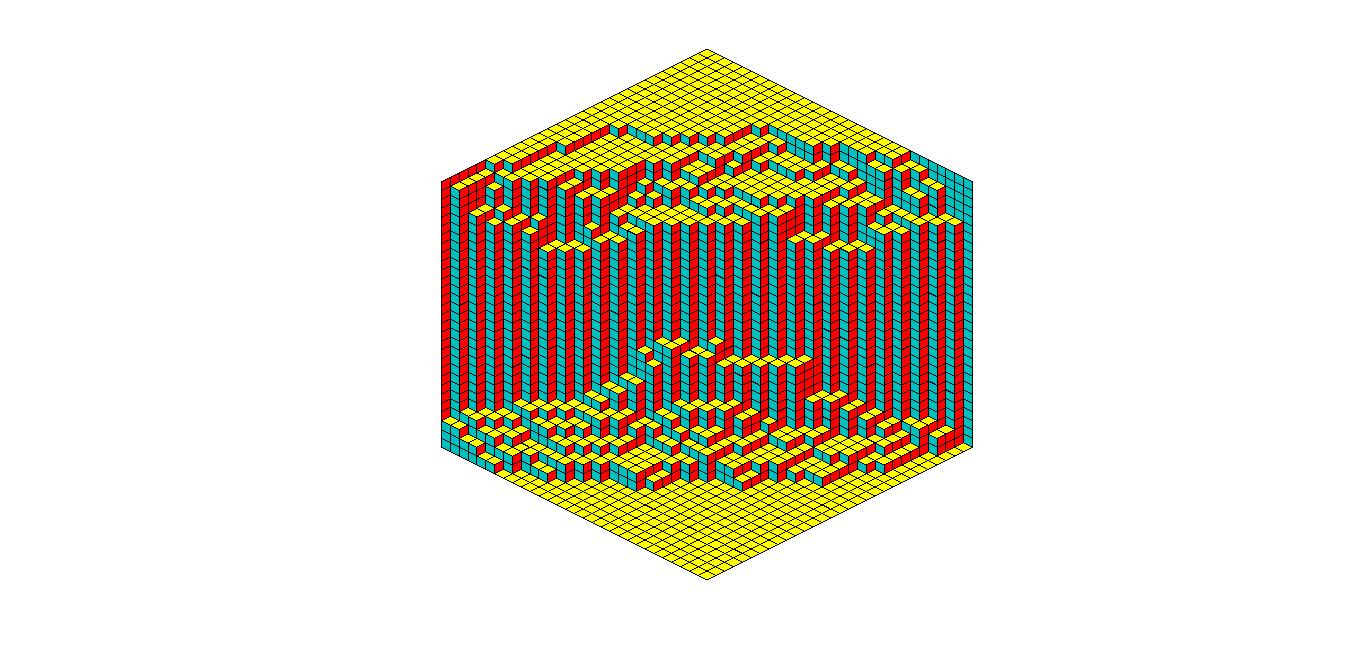
Figure 7: A typical lozenge tiling of a larger size hexagon with periodic weighting with parameter $\alpha_{j}=\alpha=1/10$ for all $j$. The regular hexagon in this picture is obtained from the one in Figure 6 by a shear transformation $(x,y)\mapsto(x,y-x/2)$. The figure is due to Christophe Charlier.

In a weighted tiling model, certain weights are assigned to the lozenges, depending on their shape and on their location in the hexagon. In a periodic weighting this is done in a periodic fashion with respect to at least one direction. The simplest model is to introduce two periodicity in one direction, say the vertical direction, depending on the location of the square tiles. In this model we fix parameters $\alpha_{1},\alpha_{2},\ldots,\alpha_{L}>0$ with $L=B+C$, and put

$$\mathcal{W}\left(\leavevmode\hbox to36.68pt{\vbox to33.43pt{\text{[drawing]}}}\right)=\begin{cases}\alpha_{j}&\text{if $x=j-1$, and $y$ is even},\\ 1&\text{if $y$ is odd},\end{cases} (x,y) (x,y)$$ (3.1)

while all other tiles have weight $1$. A hexagon tiling $\mathcal{T}$ then has the weight

$$\mathcal{W}(\mathcal{T})=\prod_{T\in\mathcal{T}}\mathcal{W}(T)=\prod_{j=1}^{L}\alpha_{j}^{N_{j}(\mathcal{T})}$$

where $N_{j}(\mathcal{T})$ is the number of square tiles in the $j$th column of $\mathcal{T}$ at an even height. This is a $1\times 2$-periodic tiling of the hexagon, as the weights only depend on the height of the lozenge (that is, the vertical direction). See the right panel of Figure 6 where the square tiles with weight $\alpha_{j}$ are highlighted. We introduce a probability measure $\mathbb{P}$ on the set of all tilings of a hexagon of fixed size by setting

$$\mathbb{P}(\mathcal{T})=\frac{\mathcal{W}(\mathcal{T})}{\sum_{\mathcal{T}^{\prime}}\mathcal{W}(\mathcal{T}^{\prime})},$$ (3.2)

where the sum runs over all possible tilings $\mathcal{T}^{\prime}$ of the hexagon.

There is a completely analogous weighting which is $2\times 1$ periodic. Here the weight of the square tile depends on the parity of the horizontal coordinate instead of the vertical coordinate. The two weightings are equivalent and show the same phenomena in the large size limit. The main phenomenon that was discovered is illustrated in Figure 7. In the large $n$ limit the pattern of tiles is fixed in certain regions near the corners of the hexagon, where only one type of lozenge is present, as well as in a region in the middle with two types of lozenges. These regions are called the solid regions. The remaining part of the hexagon is referred to as a liquid region. All three types of lozenges are present in the liquid region, and they do not appear in a regular pattern.

The solid region with two types of lozenges can connect two opposite sides of the hexagon as it is the case in Figure 7 or it can happen that it consists of two disjoint parts. In the former case the liquid region consists of two disjoint pieces, while in the latter case the liquid region is connected. There is a transition between the two cases which depends on the parameter $\alpha>0$. The critical parameter is $\alpha=1/9$ as shown in [7].

3.2 Systems of non-intersecting paths

A lozenge tiling of the hexagon can be alternatively viewed as a non-intersecting path system. The paths correspond to level lines for the height function for boxes stacked in a corner. The non-intersecting paths are obtained by drawing diagonal lines on two of the three types of lozenges as shown in Figure 8. This gives us a bijection between tilings of an $ABC$-hexagon and non-intersecting path systems on a directed graph $\mathcal{G}=(\mathbb{Z}^{2},E)$ with starting points at $A$ consecutive points $(0,0),\ldots,(0,A-1)$ and ending points at $(B+C,C),\ldots,(B+C,A+C-1)$. The edge set $E$ consists of directed edges $((x,y),(x+1,y))$ and $((x,y),(x+1,y+1))$ with $(x,y)\in\mathbb{Z}^{2}$. See Figure 8 for the non-intersecting path system corresponding to the tiling of Figure 6. The weights $\alpha_{j}$ on the square tiles in the $1\times 2$ periodic setting correspond to edge weights on the horizontal edges at even numbered heights. Note that we applied a shift $y\mapsto y-1/2$ to the vertical coordinate.

By then putting particles on the paths as also indicated in Figure 8, we obtain a multi-level particle system. A hexagon of size $ABC$ then has $B+C+1$ levels $0,1,\ldots,B+C$ with $A$ particles on each level. The vertical positions of the particles on the $m$th level will be denoted by

$$y_{0}^{(m)}<y_{1}^{(m)}<\cdots<y_{A-1}^{(m)}$$

with fixed starting positions $y_{j}^{(0)}=j$ and ending positions $y_{j}^{(L)}=C+j$ for $j=0,\ldots,A-1$, at levels $0$ and $B+C$, respectively.

Figure 8: The non-intersecting path system on a directed graph corresponding to the hexagon tiling of Figure 6. The $1\times 2$ periodic weighting corresponds to weights $\alpha$ on the horizontal edges at even height. All other edges have weight $1$.

To any weighting of the edges of the directed graph we associate transition matrices $T_{m}:\mathbb{Z}\times\mathbb{Z}\to\mathbb{R}$ for $m\in\mathbb{Z}$ where $T_{m}(x,y)$ is equal to the weight on the edge from $(m,x)$ to $(m+1,y)$ if there is such an edge, and zero otherwise.

Then it is a general fact, which is a consequence of the Lindström-Gessel-Viennot lemma [25, 32] that the multi-level particle system coming from an $ABC$-hexagon has the joint probability measure given by a product of determinants

$$P\left(\left(y_{j}^{(m)}\right)_{j=0,m=0}^{A-1,B+C}\right)\\ =\frac{1}{Z_{A,B,C}}\prod_{j=0}^{A-1}\delta_{j}\left(y_{j}^{(0)}\right)\cdot\prod_{m=0}^{B+C-1}\det\left[T_{m}\left(y_{j}^{(m)},y_{k}^{(m+1)}\right)\right]_{j,k=0}^{A-1}\cdot\prod_{j=0}^{A-1}\delta_{C+j}\left(y_{j}^{(B+C)}\right).$$ (3.3)

The probability measure (3.3) is determinantal by the Eynard-Mehta theorem [23] (see also [17, Theorem 4.3]) with a correlation kernel that has an explicit double sum formula.

3.3 Periodic transition matrices

One of the contributions of [17] is to rewrite the correlation kernel of the determinantal point process as a double contour integral in case all transition matrices $T_{m}$ are periodic, in the sense that

$$T_{m}(x+p,y+p)=T_{m}(x,y),\qquad(x,y)\in\mathbb{Z}^{2}$$

for some integer $p\geq 1$. The MVOP appear in this formula and they have size $p\times p$ if the transition matrices are $p$-periodic. The orthogonality weights come from the symbols of the transition matrices.

In the situation of the two periodic weighting with parameters $\alpha_{1},\ldots,\alpha_{B+C}$, the transition matrices $T_{m}:\mathbb{Z}\times\mathbb{Z}\to\mathbb{R}$ are $2$-periodic

$$T_{m}(x,y)=\begin{cases}\alpha_{j},&\text{if $m=j-1$, and $y=x$ is even},\\ 1,&\text{if $m=j-1$, and $y=x$ is odd or if $y=x+1$},\\ 0,&\text{otherwise}.\end{cases}$$ (3.4)

The symbol of $T_{m}$ is given by

$$W_{\alpha}(z)=\begin{pmatrix}\alpha&1\\ z&1\end{pmatrix},\qquad\text{with $\alpha=\alpha_{j}$, $j=m+1$}$$ (3.5)

and these will enter into the matrix-valued weight function.

The formalism of [17] then assumes that the sides $A$ and $C$ of the hexagon are even, say $A=2k$, $C=2c$. The matrix-valued orthogonality weight then is

$$\frac{W_{\alpha_{1}}(z)W_{\alpha_{2}}(z)\cdots W_{\alpha_{B+C}}(z)}{z^{k+c}},$$ (3.6)

and Lemma 4.8 of [17] then states that a unique monic matrix-valued polynomial $P_{k}$ of degree $k$ exists that is orthogonal with respect to the above weight matrix on a closed contour $\gamma$ going around $0$ once in the counterclockwise direction. This leads to the proof of the existence of MVOP.

3.4 Proof of Proposition 1.1

Proof.

Suppose an integer $k\geq 0$ is given, as well as integers $K\geq k$ and $L\geq 2(K-k)$. We take

$$A=2k,\quad c=K-k,\quad C=2c,\quad\text{and}\quad B=L-C.$$

Then $A,B,C$ are non-negative integers with $A$ and $C$ even. With these parameters the matrix weight (3.6) is equal to (1.3) and therefore the MVOP $P_{k}$ of degree $k$ uniquely exists, due to [17, Lemma 4.8]. ∎

4 Proof of Theorem 1.2

Proof.

(a) Let

$$Q_{2k}(\zeta)=P_{k}(\zeta^{2}-\beta^{2})\begin{pmatrix}1&1\\ \zeta+\beta&-\zeta+\beta\end{pmatrix}.$$ (4.1)

Then the first column of $Q_{2k}$ has the entries

$$q_{2k}(\zeta):=\left(Q_{2k}\right)_{11}(\zeta) =\left(P_{k}\right)_{11}(\zeta^{2}-\beta^{2})+\left(P_{k}\right)_{12}(\zeta^{2}-\beta^{2})(\zeta+\beta),$$ (4.2)

$$q_{2k+1}(\zeta):=\left(Q_{2k}\right)_{21}(\zeta) =\left(P_{k}\right)_{21}(\zeta^{2}-\beta^{2})+\left(P_{k}\right)_{22}(\zeta^{2}-\beta^{2})(\zeta+\beta),$$

and these are easily seen to be monic polynomials of respective degrees $2k$ and $2k+1$, since $P_{k}$ is a monic matrix valued polynomial of degree $k$. From (4.1) it is also immediate that the second column contains the entries $q_{2k}(-\zeta)$ and $q_{2k+1}(-\zeta)$ with the same polynomials (4.2). Thus (1.6) holds and it remains to check the orthogonality (1.7).

The matrix orthogonality of $P_{k}$ with weight (1.5) yields

$$\frac{1}{2\pi i}\oint_{\gamma}P_{k}(z)W_{\alpha}(z)^{L}z^{j-K}dz=0_{2},\quad j=0,1,\ldots,k-1,$$ (4.3)

where we choose for $\gamma$ the circle around $-\beta^{2}$ of radius $R^{2}>\beta^{2}$. Recall the spectral decomposition $W_{\alpha}=E\Lambda E^{-1}$ from (1.11) with

$$\Lambda(\zeta) =\begin{pmatrix}\zeta+\alpha+\beta&0\\ 0&-\zeta+\alpha+\beta\end{pmatrix},\qquad E(\zeta)=\begin{pmatrix}1&1\\ \zeta+\beta&-\zeta+\beta\end{pmatrix},$$ (4.4)

and $\zeta=(z+\beta^{2})^{1/2}$, $\operatorname{Re}\zeta>0$, see (1.12) and (1.13). Hence by (4.1), (1.11), (4.4),

$$P_{k}(z)W_{\alpha}(z)^{L} =Q_{2k}(\zeta)\Lambda(\zeta)^{L}E^{-1}(\zeta)=Q_{2k}(\zeta)\Lambda(\zeta)^{L}\frac{1}{2\zeta}\begin{pmatrix}\zeta&1\\ \zeta&-1\end{pmatrix}\begin{pmatrix}1&0\\ -\beta&1\end{pmatrix}.$$

Performing the change of variable $z=\zeta^{2}-\beta^{2}$ with $dz=2\zeta d\zeta$ in (4.3), we obtain

$$\frac{1}{2\pi i}\int_{\gamma_{R}^{+}}Q_{2k}(\zeta)\Lambda(\zeta)^{L}\begin{pmatrix}\zeta&1\\ \zeta&-1\end{pmatrix}\begin{pmatrix}1&0\\ -\beta&1\end{pmatrix}(\zeta^{2}-\beta^{2})^{j-K}d\zeta=0_{2},\quad j=0,1,\ldots,k-1,$$ (4.5)

where $\gamma_{R}^{+}$ denotes the semicircle $|\zeta|=R$, $\operatorname{Re}\zeta>0$. The constant matrix $\begin{pmatrix}1&0\\ -\beta&1\end{pmatrix}$ can be dropped from (4.5) as it disappears if we multiply by its inverse. Then the matrix identity (4.5) results in four integrals that are equal to zero, and each integral contains the scalar weight $w_{\alpha,K,L}$ from (1.10). Using (4.1), (1.6), (4.4), and (1.10), we obtain the following integrals containing either $q_{2k}$ or $q_{2k+1}$,

$$\begin{aligned} \frac{1}{2\pi i}\int_{\gamma_{R}^{+}}\left[q_{2k+\epsilon}(\zeta)w_{\alpha,K,L}(\zeta)+q_{2k+\epsilon}(-\zeta)w_{\alpha,K,L}(-\zeta)\right]\,\zeta(\zeta^{2}-\beta^{2})^{j}d\zeta&=0,\\ \frac{1}{2\pi i}\int_{\gamma_{R}^{+}}\left[q_{2k+\epsilon}(\zeta)w_{\alpha,K,L}(\zeta)-q_{2k+\epsilon}(-\zeta)w_{\alpha,K,L}(-\zeta)\right]\,(\zeta^{2}-\beta^{2})^{j}d\zeta&=0,\end{aligned}$$ (4.6)

for $\epsilon=0,1$, and $j=0,1,\ldots,k-1$.

The integrals in (4.6) are turned into integrals over the full circle $\gamma_{R}$ by writing them as a sum of two integrals and changing variables $\zeta\to-\zeta$ in the second one. We obtain for $j=0,1,\ldots,k-1$, and $\epsilon=0,1$,

$$\frac{1}{2\pi i}\oint_{\gamma_{R}}q_{2k+\epsilon}(\zeta)w_{\alpha,K,L}(\zeta)\zeta(\zeta^{2}-\beta^{2})^{j}d\zeta =0,$$ (4.7)

$$\frac{1}{2\pi i}\oint_{\gamma_{R}}q_{2k+\epsilon}(\zeta)w_{\alpha,K,L}(\zeta)(\zeta^{2}-\beta^{2})^{j}d\zeta =0.$$

Observe the extra factor $\zeta$ in the first integral of (4.7). The $2k$ polynomials $\zeta\mapsto\zeta(\zeta^{2}-\beta^{2})^{j}$, $\zeta\mapsto(\zeta^{2}-\beta^{2})^{j}$, $j=0,\ldots,k-1$, are linearly independent, since we have a unique polynomial in this set for each degree from $0$ up to $2k-1$. Thus they are a basis of the vector space of all polynomials of degree $\leq 2k-1$. We then obtain (1.7) by taking suitable linear combinations of the identities in (4.7), which completes the proof of part (a).

(b) Suppose $q_{2k}$ and $q_{2k+1}$ are two monic polynomials of degrees $2k$ and $2k+1$, respectively that satisfy (1.7) and define $Q_{2k}$ as

$$Q_{2k}(\zeta)=\begin{pmatrix}q_{2k}(\zeta)&q_{2k}(-\zeta)\\ q_{2k+1}(\zeta)&q_{2k+1}(-\zeta)\end{pmatrix}.$$

Then, for any $c\in\mathbb{C}$, the matrix valued function $P_{k}$ as defined in (1.9) satisfies the orthogonality (1.1) with weight matrix (1.5), simply by reversing the arguments from part (a). From the second line of (1.9) it is clear that $P_{k}$ is a polynomial in the variable $z$, see also the remark following the statement of Theorem 1.2. The diagonal entries of $P_{k}$ are monic polynomials of degree $k$, and the $(1,2)$-entry is a polynomial of degree $\leq k-1$. The $(2,1)$-entry is a polynomial of degree $\leq k$.

Suppose

$$q_{2k+1}(\zeta)=\zeta^{2k+1}+a\zeta^{2k}+O(\zeta^{2k-1})$$

as $\zeta\to\infty$. Then

$$\frac{q_{2k+1}(\zeta)+q_{2k+1}(-\zeta)}{2}=a\zeta^{2k}+O(\zeta^{2k-2})$$

and it follows from (1.9) that

$$\left(P_{k}\right)_{21}(z)=(c+a-\beta)z^{k}+O(z^{k-1})\quad\text{as }z\to\infty.$$

The choice for $c$ in (1.18) then guarantees that $c+a-\beta=0$ and therefore the $(2,1)$ entry of $P_{k}$ has degree $\leq k-1$. Thus $P_{k}$ defined by (1.9) is a monic matrix valued polynomial with the required matrix orthogonality. Part (b) then follows because of the uniqueness of the MVOP, see also Proposition 1.1. ∎

5 Proofs of Proposition 2.3 and Theorem 2.4

We prove part (a) of Proposition 2.3 via the Deift-Zhou steepest descent analysis of the Riemann-Hilbert problem (or RH problem) for scalar orthogonal polynomials. It is well-known that the monic scalar orthogonal polynomials can be expressed in terms of a RH problem [24]. The Deift-Zhou steepest descent analysis was first performed in [14] and its application to orthogonal polynomials has been well-developed by now. We refer to [12, 13] or [3, Section 2.4] for more background information.

In our case, the method works smoothly for $q_{n,n}$ but we need a little twist to make it work for $q_{n+k,n}$ with $k\neq 0$. This is the reason why we give a detailed account here.

5.1 The Riemann-Hilbert problem for $q_{n+k,n}$

The critical trajectory $\Sigma_{0}$ is analytically continued to a closed contour $\gamma_{0}$ around $0$ as in Figure 9. The additional part is an orthogonal trajectory of the quadratic differential $Q_{\alpha}dz^{2}$. Then $\gamma_{0}$ surrounds the points $\pm\beta$, see also [7, section 4]. Thus $\gamma_{R}$ can be deformed to $\gamma_{0}$ in (2.2) without crossing the poles, and $q_{n+k,n}$ is also characterized by the orthogonality

$$\frac{1}{2\pi i}\oint_{\gamma_{0}}q_{n+k,n}(z)z^{j}\frac{(z+\alpha+\beta)^{2n}}{(z^{2}-\beta^{2})^{n}}dz=0,\qquad j=0,1,\ldots,n+k-1.$$

The closed contour $\gamma_{0}$ is positively (counterclockwise) oriented. As usual in RH problems the $+$ side is on the left and the $-$ side is on the right when traversing the contour according to its orientation.

\begin{overpic}[scale={0.7}]{Figure9.png} \put(83.0,57.0){$\Sigma_{0}$} \put(8.0,43.0){$\gamma_{0}$} \put(31.0,55.0){$z_{+}$} \put(30.0,10.0){$z_{-}$} \put(0.0,28.0){$-\alpha-\beta$} \put(20.0,28.0){$-\beta$} \put(75.0,28.0){$\beta$} \end{overpic}

Figure 9: $\Sigma_{0}$ (in blue) has analytic continuation to a closed contour $\gamma_{0}$ surrounding $\pm\beta$, where $\gamma_{0}\setminus\Sigma_{0}$ consists of orthogonal trajectories connecting $z_{\pm}$ with $-\alpha-\beta$.

Riemann-Hilbert problem 1.

$Y$ is a $2\times 2$ matrix-valued function that satisfies

• $Y:\mathbb{C}\setminus\gamma_{0}\to\mathbb{C}^{2\times 2}$ is analytic,

• $Y$ has a jump on $\gamma_{0}$ given by

  $$Y_{+}(z)=Y_{-}(z)\begin{pmatrix}1&w_{\alpha}(z)^{n}\\ 0&1\end{pmatrix}\quad\text{ for }z\in\gamma_{0},$$ (5.1)

  where $Y_{\pm}$ denote the limiting values of $Y$ on the $\pm$ sides of $\gamma_{0}$, and

  $$w_{\alpha}(z)=\frac{(z+\alpha+\beta)^{2}}{(z^{2}-\beta^{2})}.$$

• $Y(z)=(I_{2}+O(z^{-1}))\begin{pmatrix}z^{n+k}&0\\ 0&z^{-n-k}\end{pmatrix}$ as $z\to\infty$.

Fokas, Its and Kitaev first established in [24] that 1 has a solution in terms of the scalar orthogonal polynomials $q_{n+k,n}$. The solution to the RH problem exists if and only if $q_{n+k,n}$ uniquely exists, and in that case

$$Y(z)=\begin{pmatrix}q_{n+k,n}(z)&\displaystyle\frac{1}{2\pi i}\oint_{\gamma_{0}}\frac{q_{n+k,n}(s)w_{\alpha}(s)^{n}}{s-z}\text{d}s\\ \widehat{q}_{n+k-1,n}(z)&\displaystyle\frac{1}{2\pi i}\oint_{\gamma_{0}}\frac{\widehat{q}_{n+k-1,n}(s)w_{\alpha}(s)^{n}}{s-z}\text{d}s\end{pmatrix}$$ (5.2)

for some polynomial $\widehat{q}_{n+k-1,n}$ of degree $\leq n+k-1$. If $\widehat{q}_{n+k-1,n}$ has exact degree $n+k-1$, then it is a multiple of the monic orthogonal polynomial of degree $n+k-1$, and $q_{n+k-1,n}$ uniquely exists as well. However, it is possible that the degree of $\widehat{q}_{n+k-1,n}$ is less than $n+k-1$.

A consequence of the steepest descent analysis will be that, for a fixed $k\in\mathbb{Z}$, the 1 is solvable for $n$ large enough. Hence the polynomial $q_{n+k,n}$ exists for $n$ large enough.

5.2 Steepest descent analysis

5.2.1 First transformation $Y\mapsto T$

Note that there is a discrepancy between the power of the weight function in the jump of $Y$ and the degree of $z^{\pm(n+k)}$ in the asymptotics of $Y(z)$ as $z\to\infty$. The transformation $Y\mapsto T$ will not depend on $k$, and it leads to a RH problem that is not normalized at infinity, as we will see. We use the $g$-function (2.8), the function

$$V_{\alpha}(z)=-\log w_{\alpha}(z)=\log(z^{2}-\beta^{2})-2\log(z+\alpha+\beta),$$ (5.3)

as well as the following lemma.

Lemma 5.1.

Let $\frac{1}{9}<\alpha\leq 1$, and let $\Sigma_{0}$ and $\gamma_{0}$ be as in Figure 9. Then there is a constant $\ell$ such that

$$g_{+}(z)+g_{-}(z)-V_{\alpha}(z)\begin{cases}=-\ell,&z\in\Sigma_{0},\\ <-\ell,&z\in\gamma_{0}\setminus\Sigma_{0}.\end{cases}$$ (5.4)

In addition

$$g_{+}(z)-g_{-}(z)=2\phi_{+}(z),\qquad z\in\Sigma_{0},$$ (5.5)

where $\phi$ is defined by

$$\phi(z)=\int_{z_{+}}^{z}Q_{\alpha}(s)^{1/2}ds$$ (5.6)

and $\phi$ satisfies

$$\phi(z)=g(z)-\frac{V_{\alpha}(z)}{2}+\frac{\ell}{2},\qquad z\in\mathbb{C}\setminus(\Sigma_{0}\cup(-\infty,x^{*}])$$ (5.7)

where $x^{*}$ is the point of intersection of $\Sigma_{0}$ with the positive real line.

Proof.

This is essentially the same as the proof of [7, Proposition 4.4]. ∎

By taking the derivative in (5.7) and using (5.6) we get that

$$2g^{\prime}(z)=V_{\alpha}^{\prime}(z)+2Q_{\alpha}(z)^{1/2},\qquad z\in\mathbb{C}\setminus\Sigma_{0}.$$ (5.8)

Also note that $\mu_{0}$ is a critical measure in the sense of Martínez-Finkelshtein and Rakhmanov, see [33] and especially Section 5 therein.

We then define

$$T(z)=e^{\frac{n\ell}{2}\sigma_{3}}Y(z)e^{-ng(z)\sigma_{3}}e^{-\frac{n\ell}{2}\sigma_{3}},\qquad\quad\sigma_{3}=\begin{pmatrix}1&0\\ 0&-1\end{pmatrix}.$$ (5.9)

Then $T$ satisfies the following Riemann-Hilbert problem.

Riemann-Hilbert problem 2.

The matrix valued function $T$ satisfies the following:

• $T:\mathbb{C}\setminus\gamma_{0}\to\mathbb{C}^{2\times 2}$ is analytic,

• $T$ has boundary values on $\gamma_{0}$ that satisfy

  $$T_{+}(z) =T_{-}(z)\begin{pmatrix}e^{-2n\phi_{+}(z)}&1\\ 0&e^{-2n\phi_{-}(z)}\end{pmatrix}, z\in\Sigma_{0}\subset\gamma_{0}$$ for , (5.10)

  $$T_{+}(z) =T_{-}(z)\begin{pmatrix}1&e^{2n\phi(z)}\\ 0&1\end{pmatrix}, z\in\gamma_{0}\setminus\Sigma_{0}$$ for , (5.11)

• $T(z)=\left(I_{2}+O(z^{-1})\right)\begin{pmatrix}z^{k}&0\\ 0&z^{-k}\end{pmatrix}$ as $z\to\infty$.

The jump matrix on $\gamma_{0}\setminus\Sigma_{0}$ tends to the identity matrix as $n\to\infty$ because $\phi(z)<0$ on $\gamma_{0}\setminus\Sigma_{0}$ due to (5.7) and the strict inequality in (5.4).

5.2.2 Second transformation $T\mapsto S$: opening of lenses

We open up lenses around $\Sigma_{0}$ such that $\operatorname{Re}\phi>0$ on the lips $\gamma_{+}$ and $\gamma_{-}$ of the lenses, except at the endpoints $z_{+},z_{-}$, and we define

$$S(z)=T(z)\times\begin{cases}\begin{pmatrix}1&0\\ -e^{-2n\phi(z)}&1\end{pmatrix}&\text{for $z$ between $\Sigma_{0}$ and $\gamma_{+}$},\\ \begin{pmatrix}1&0\\ e^{-2n\phi(z)}&1\end{pmatrix}&\text{for $z$ between $\Sigma_{0}$ and $\gamma_{-}$},\\ I_{2}&\text{elsewhere}.\end{cases}$$ (5.12)

Then $S$ satisfies the following Riemann-Hilbert problem:

Riemann-Hilbert problem 3.

The function $S$ satisfies:

• $S:\mathbb{C}\setminus(\gamma\cup\gamma_{+}\cup\gamma_{-})\to\mathbb{C}^{2\times 2}$ is analytic,

• $S$ has boundary values on $\gamma$, $\gamma_{+}$ and $\gamma_{-}$ that satisfy

  $$S_{+}(z) =S_{-}(z)\begin{pmatrix}1&0\\ e^{-2n\phi(z)}&1\end{pmatrix} \text{for $z\in\gamma_{+}\cup\gamma_{-}$},$$ (5.13)

  $$S_{+}(z) =S_{-}(z)\begin{pmatrix}0&1\\ -1&0\end{pmatrix} \text{for $z\in\Sigma_{0}$},$$ (5.14)

  $$S_{+}(z) =S_{-}(z)\begin{pmatrix}1&e^{2n\phi(z)}\\ 0&1\end{pmatrix} \text{for $z\in\gamma_{0}\setminus\Sigma_{0}$},$$ (5.15)

• $S(z)=(I_{2}+O(z^{-1}))\begin{pmatrix}z^{k}&0\\ 0&z^{-k}\end{pmatrix}$ as $z\to\infty$.

The jump matrices on $\gamma_{\pm}$ and on $\gamma_{0}\setminus\Sigma_{0}$ tend to the identity matrix as $n\to\infty$.

5.2.3 Model Riemann-Hilbert problem

Ignoring the jumps that are exponentially small, we look for a solution $N$ to the following model Riemann-Hilbert problem:

Riemann-Hilbert problem 4.

The function $N$ satisfies

• $N:\mathbb{C}\setminus\Sigma_{0}\to\mathbb{C}^{2\times 2}$ is analytic,

• $N$ has boundary values on $\Sigma_{0}$ that satisfy

  $$N_{+}(z)=N_{-}(z)\begin{pmatrix}0&1\\ -1&0\end{pmatrix}\quad\text{ for }z\in\Sigma_{0},$$ (5.16)

• $N(z)=\left(I_{2}+O(z^{-1})\right)\begin{pmatrix}z^{k}&0\\ 0&z^{-k}\end{pmatrix}$ as $z\to\infty$.

The 4 depends on the integer $k\in\mathbb{Z}$ as it appears in the asymptotic condition.

The solution $N_{0}$ for the case $k=0$ is well-known, namely

$$N_{0}(z)=\begin{pmatrix}\displaystyle\frac{1}{2}(a(z)+a(z)^{-1})&\displaystyle\frac{1}{2i}(a(z)-a(z)^{-1})\\[5.0pt] \displaystyle-\frac{1}{2i}(a(z)-a(z)^{-1})&\displaystyle\frac{1}{2}(a(z)+a(z)^{-1})\end{pmatrix},$$ (5.17)

where $a(z)$ is given by (2.10). Note that $(N_{0})_{11}(z)=A_{0}(z)$ where $A_{0}(z)$ is given by (2.9).

Lemma 5.2.

The solution of 4 takes the form

$$N(z)=\begin{pmatrix}c^{k}&0\\ 0&c^{-k}\end{pmatrix}N_{0}(z)\begin{pmatrix}\left(\frac{\psi(z)}{c}\right)^{k}&0\\ 0&\left(\frac{\psi(z)}{c}\right)^{-k}\end{pmatrix}$$ (5.18)

where $c=\frac{z_{+}-z_{-}}{4}$ and $\psi(z)$ is given by (2.11).

Proof.

The function $\psi$ is analytic and non-zero on $\mathbb{C}\setminus\Sigma_{0}$ with boundary values satisfying $\psi_{+}\psi_{-}=c^{2}$ on $\Sigma_{0}$, as can be easily obtained from (2.11). These properties guarantee that $N$ is well-defined and analytic outside $\Sigma_{0}$ with the same jump matrix on $\Sigma_{0}$ as $N_{0}$ has. Also $\psi(z)=z+O(1)$ as $z\to\infty$ and this gives the asymptotic condition from the 4. ∎

5.2.4 Local parametrices and final transformation $S\mapsto R$

In small disks $D_{+}$ and $D_{-}$ around the endpoints $z_{+}$ and $z_{-}$ of $\Sigma_{0}$, we can build local parametrices using Airy functions, see for example [12, 13] or [3, Section 2.4.6]. We will call these $P^{(+)}$ and $P^{(-)}$ respectively. The local parametrices do not play a role in the strong asymptotics of $q_{n+k,n}$ away from the contour $\Sigma_{0}$.

We next define the function $R$ by

$$R(z)=S(z)\times\begin{cases}N(z)^{-1}&\text{ for }z\in\mathbb{C}\setminus(D_{+}\cup D_{-}),\\ P^{(+)}(z)^{-1}&\text{ for }z\in D_{+},\\ P^{(-)}(z)^{-1}&\text{ for }z\in D_{-}.\end{cases}$$ (5.19)

Then the following lemma holds, cf.  [3, Section 2.5] or [31, Lemma 8.3].

Lemma 5.3.

$R$ is the solution of a small-norm RH problem, which has a solution for $n$ large enough. In addition, there exists a constant $C>0$ such that for all $z\in\mathbb{C}$,

$$\|R(z)-I_{2}\|\leq\frac{C}{n(1+|z|)},$$

where $\|\cdot\|$ denotes any matrix norm.

5.2.5 Proof of Proposition 2.3(a)

Since $R$ exists for $n$ large enough, we find by tracing back the transformations $Y\mapsto T\mapsto S\mapsto R$ that the 1 is solvable for $n$ large enough. This implies that $q_{n+k,n}$ exists for $n$ large enough.

Let $K$ be a compact subset of $\overline{\mathbb{C}}\setminus\Sigma_{0}$. By taking the lense around $\Sigma_{0}$ and the disks around $z_{\pm}$ small enough such that $K$ lies outside the region bounded by the lenses and disks, we find from (5.9), (5.12), (5.19) that

$$Y(z)=e^{-\frac{n\ell}{2}\sigma_{3}}R(z)N(z)e^{\frac{n\ell}{2}\sigma_{3}}e^{ng(z)\sigma_{3}},\quad z\in K.$$

Because $q_{n+k,n}(z)=Y_{11}(z)$ is the $(1,1)$-entry of $Y$ we then obtain

$$q_{n+k,n}(z) =\begin{pmatrix}1&0\end{pmatrix}Y(z)\begin{pmatrix}1\\ 0\end{pmatrix}$$

$$=e^{ng(z)}\begin{pmatrix}1&0\end{pmatrix}R(z)N(z)\begin{pmatrix}1\\ 0\end{pmatrix}$$

$$=e^{ng(z)}\left(R_{11}(z)N_{11}(z)+R_{12}(z)N_{21}(z)\right),\qquad z\in K.$$

Using Lemma 5.3, we calculate

$$q_{n+k,n}(z) =e^{ng(z)}\left(N_{11}(z)\left(1+O\left(\frac{1}{n(1+|z|)}\right)\right)+N_{12}(z)O\left(\frac{1}{n(1+|z|)}\right)\right)$$

$$=N_{11}(z)e^{ng(z)}\left(1+O\left(\frac{1}{n(1+|z|)}\right)\right),\qquad z\in K.$$

with $O$ term that is uniform on $K$. The second identity holds since $|N_{11}(z)|$ is bounded away from $0$ for $z\in K$. Then part (a) of Proposition 2.3 follows since the $(1,1)$ entry of $N$ satisfies

$$N_{11}(z)=A_{0}(z)\psi(z)^{k}$$

see (5.17) and (5.18).

5.3 Proof of Proposition 2.3(b)

Part (b) follows from the strong asymptotic formula (2.12) in a standard fashion. Indeed, (2.12) implies that

$$\lim_{n\to\infty}\frac{1}{n}\log|q_{n,n}(z)|=\operatorname{Re}g(z),\qquad z\in\mathbb{C}\setminus\Sigma_{0}$$

and $\operatorname{Re}g=-U^{\mu_{0}}$ where

$$U^{\mu_{0}}(z)=\int\log\frac{1}{|z-s|}d\mu_{0}(s)$$

is the logarithmic potential of $\mu_{0}$. Part (b) then follows from the following result that is well-known, but we state it here for convenience, as we will also use it in later proofs.

Lemma 5.4.

Suppose $(p_{n})_{n}$ is a sequence of monic polynomials with $\deg p_{n}=n$ whose zeros are all in a bounded subset of the complex plane. Suppose $\mu$ is a probability measure with compact support such that

$$\lim_{n\to\infty}\frac{1}{n}\log|p_{n}(z)|=-U^{\mu}(z),\qquad\text{ a.e.\ on }\mathbb{C}.$$ (5.20)

Then the sequence $(\nu(p_{n}))_{n}$ of normalized zero counting measures tends to $\mu$ in the weak sense.

Proof.

Let $\nu_{n}=\nu(p_{n})$ the normalized counting measure of the zeros of $p_{n}$, see (2.13). The proof that $\mu_{0}$ is the weak limit of $(\nu_{n})_{n}$ as $n\to\infty$ uses basic tools from logarithmic potential theory.

The probability measures $\nu_{n}$ are all supported on a fixed compact subset $K$ of $\mathbb{C}$. The set of probability measures on $K$ is compact for the weak topology. Thus, by a standard compactness argument, it suffices to show that $\mu$ is the only possible limit of a weakly convergent subsequence.

Suppose $(\nu_{n_{j}})_{j}$ is a subsequence of $(\nu_{n})_{n}$ that weakly converges to some probability measure $\nu$ on $K$. Then by the Lower Envelope Theorem, see [38, Theorem I.6.9] one has

$$\lim_{j\to\infty}U^{\nu_{n_{j}}}(z)=U^{\nu}(z),\quad\text{ for quasi-every }z\in\mathbb{C}.$$

Here quasi-every $z$ means except for a set of capacity zero, and in particular it holds almost everywhere with respect to two-dimensional Lebesgue measure. Because of (5.20) and

$$U^{\nu_{n}}(z)=-\frac{1}{n}\log|p_{n}(z)|$$

we then find that $U^{\mu}(z)=U^{\nu}(z)$ a.e. on $\mathbb{C}$. The uniqueness theorem for logarithmic potentials, see [38, Theorem II.2.1] then implies that $\nu=\mu$. This proves the lemma. ∎

The proof of Proposition 2.3(b) clearly also works for the zeros of $q_{n+k,n}$ as $n\to\infty$ with a fixed $k\in\mathbb{Z}$.

5.4 Proof of Theorem 2.4

From (2.16) and the strong asymptotic formula (2.12) that we use for $k=0$ and $k=1$, we obtain

$$\det P_{n,n}(\zeta^{2}-\beta^{2}) =\frac{1}{2\zeta}(q_{2n,2n}(\zeta)q_{2n+1,2n}(-\zeta)-q_{2n,2n}(-\zeta)q_{2n+1,2n}(\zeta))$$

$$=\frac{1}{2\zeta}A_{0}(\zeta)A_{0}(-\zeta)e^{2n(g(\zeta)+g(-\zeta))}$$

$$\qquad\times\left(\psi(-\zeta)\left(1+O\left(\frac{1}{n(1+|\zeta|)}\right)\right)-\psi(\zeta)\left(1+O\left(\frac{1}{n(1+|\zeta|)}\right)\right)\right)$$

$$=A_{0}(\zeta)A_{0}(-\zeta)\frac{\psi(-\zeta)-\psi(\zeta)}{2\zeta}e^{2n(g(\zeta)+g(-\zeta))}\left(1+O\left(\frac{1}{n(1+|\zeta|)}\right)\right)$$ (5.21)

as $n\to\infty$, uniformly for $\zeta$ in compact subsets of $\overline{\mathbb{C}}\setminus(\Sigma_{0}\cup-\Sigma_{0})$. We may indeed combine the two $O$ terms in the last step of (5.21) since $\psi(-\zeta)-\psi(\zeta)$ does not vanish in $\mathbb{C}\setminus(\Sigma_{0}\cup-\Sigma_{0})$.

Thus the zeros of $\zeta\mapsto\det P_{n,n}(\zeta^{2}-\beta^{2})$ tend to $\Sigma_{0}\cup-\Sigma_{0}$ as $n\to\infty$, which means that the zeros of $\det P_{n,n}$ tend to $\widetilde{\Sigma}_{0}$, see (2.14).

Using (5.21) we also find for $\zeta\in\mathbb{C}\setminus(\Sigma_{0}\cup-\Sigma_{0})$,

$$\lim_{n\to\infty}\frac{1}{2n}\log\left|\det P_{n,n}(\zeta^{2}-\beta^{2})\right| =\operatorname{Re}\left(g(\zeta)+g(-\zeta)\right)$$

$$=\int\log|\zeta-s|d\mu_{0}(s)+\int\log|\zeta+s|d\mu_{0}(s)$$

$$=\int\log|\zeta^{2}-s^{2}|d\mu_{0}(s)$$

and therefore for $z\in\mathbb{C}\setminus\widetilde{\Sigma}_{0}$,

$$\lim_{n\to\infty}\frac{1}{2n}\log\left|\det P_{n,n}(z)\right| =\int\log\left|z-(s^{2}-\beta^{2})\right|d\mu_{0}(s)=-U^{\widetilde{\mu}_{0}}(z),$$

see also (2.15). Since $\det P_{n,n}$ is a monic polynomial of degree $2n$ we can apply Lemma 5.4 and Theorem 2.4 follows.

6 Proof of Theorem 2.5

Throughout this section we assume that the inequality (2.18) for the $g$-function holds. We write

$$Q_{n}(z)=\frac{q_{n,n}(z)-q_{n,n}(-z)}{2z},$$ (6.1)

which is a polynomial of degree

$$d_{n}=\deg Q_{n}\leq n-1.$$

We let $\nu(Q_{n})$ be its normalized zero counting measure.

Lemma 6.1.

1. The a priori signed measure $\nu$ defined by (2.19) is a probability measure with

   $$U^{\nu}(z)=\min\left(U^{\mu_{0}}(z),U^{\mu_{0}}(-z)\right)=\begin{cases}U^{\mu_{0}}(z),&z\in{\operatorname{LHP}},\\ U^{\mu_{0}^{*}}(z),&z\in{\operatorname{RHP}}.\end{cases}$$ (6.2)

2. We have

   $$\lim_{n\to\infty}-\frac{1}{n}\log|Q_{n}(z)|=U^{\nu}(z),\qquad z\in\mathbb{C}\setminus(i\mathbb{R}\cup\Sigma_{0}\cup-\Sigma_{0}),$$ (6.3)

   where the convergence is uniform in compacts of $\mathbb{C}\setminus(i\mathbb{R}\cup\Sigma_{0}\cup-\Sigma_{0})$.

3. The zeros of $Q_{n}$ tend to $i\mathbb{R}\cup\Sigma_{0}\cup-\Sigma_{0}$ or to $\infty$ as $n\to\infty$.

Proof.

(a) The inequality (2.18) tells us that

$$U^{\mu_{0}}(z)>U^{\mu_{0}}(-z)=U^{\mu_{0}^{*}}(z),\qquad z\in{\operatorname{RHP}}$$ (6.4)

where $\mu_{0}^{*}$ is the reflection of $\mu_{0}$ in the imaginary axis. Because of symmetry we have the opposite inequality in the left half-plane and equality on the imaginary axis. This proves the second equality in (6.2).

Write $\mu_{0}=\mu_{R}+\mu_{L}$ with $\mu_{R}=\mu_{0}|_{{\operatorname{RHP}}}$, $\mu_{L}=\mu_{0}|_{{\operatorname{LHP}}}$, and similarly $\mu_{0}^{*}=\mu^{*}_{R}+\mu^{*}_{L}$. By the properties of balayage, we have $U^{\mu_{L}}(z)=U^{\operatorname{Bal}(\mu_{L})}(z)$ and $U^{\mu^{*}_{L}}(z)=U^{\operatorname{Bal}(\mu^{*}_{L})}(z)$ for $z\in{\operatorname{RHP}}$, and then (6.4) gives

$$U^{\mu_{R}}(z)+U^{\operatorname{Bal}(\mu_{L})}(z)>U^{\mu_{R}^{*}}(z)+U^{\operatorname{Bal}(\mu_{L}^{*})}(z),\qquad z\in{\operatorname{RHP}}$$ (6.5)

with equality for $\operatorname{Re}z=0$. Both sides of (6.5) are harmonic in the left half-plane, and behave like ${-\log|z|+O(z^{-1})}$ as $|z|\to\infty$. Since they are equal on the imaginary axis, we obtain equality in the left half-plane by the maximum principle for harmonic functions, that is,

$$U^{\mu_{R}}(z)+U^{\operatorname{Bal}(\mu_{L})}(z)=U^{\mu_{R}^{*}}(z)+U^{\operatorname{Bal}(\mu^{*}_{L})}(z),\quad z\in\overline{{\operatorname{LHP}}}.$$ (6.6)

We next use De La Vallée Poussin’s theorem from potential theory which is stated in [38, Theorem IV 4.5] for measures with compact supports, and is extended to measures with unbounded support in [36, Theorem 4.9]. We obtain from (6.5) and (6.6) that

$$\left(\mu_{R}+\operatorname{Bal}(\mu_{L})\right)|_{\overline{{\operatorname{LHP}}}}\leq\left(\mu^{*}_{R}+\operatorname{Bal}(\mu^{*}_{L})\right)|_{\overline{{\operatorname{LHP}}}}.$$

Since $\mu_{R}$ and $\mu^{*}_{R}$ are supported in the open right half-plane and the balayage measures are on the imaginary axis, we conclude

$$\operatorname{Bal}(\mu_{L})\leq\operatorname{Bal}(\mu^{*}_{L})$$

By symmetry we have $\operatorname{Bal}(\mu_{R})=\operatorname{Bal}(\mu^{*}_{L})$ and we find $\nu_{0}=\operatorname{Bal}(\mu_{R})-\operatorname{Bal}(\mu_{L})\geq 0$. Then also $\nu=\mu_{L}+\mu_{R}^{*}+\nu_{0}\geq 0$ is a positive measure.

Furthermore

$$U^{\nu}=U^{\mu_{L}}+U^{\mu_{R}^{*}}+U^{\operatorname{Bal}(\mu_{R})}-U^{\operatorname{Bal}(\mu_{L})}.$$

In the right half-plane we have $U^{\operatorname{Bal}(\mu_{L})}=U^{\mu_{L}}$, and $U^{\operatorname{Bal}(\mu_{R})}=U^{\operatorname{Bal}(\mu_{L}^{*})}=U^{\mu_{L}^{*}}$, and we find $U^{\nu}=U^{\mu_{R}^{*}}+U^{\mu_{L}^{*}}=U^{\mu_{0}^{*}}$ in the right half-plane. Similarly $U^{\nu}=U^{\mu_{0}}$ in the left half-plane and the first equality in (6.2) follows. The equality implies that

$$U^{\nu}(z)=-\log|z|+O(1)\qquad\text{ as }z\to\infty,$$

and therefore $\nu$ has total mass one, i.e., it is a probability measure.

(b) The asymptotic formula (2.12) implies that

$$\lim_{n\to\infty}\frac{1}{n}\log|q_{n,n}(z)| =\operatorname{Re}g(z),\qquad z\in\mathbb{C}\setminus\Sigma_{0},$$

$$\lim_{n\to\infty}\frac{1}{n}\log|q_{n,n}(-z)| =\operatorname{Re}g(-z),\qquad z\in\mathbb{C}\setminus-\Sigma_{0},$$

where the convergence is uniform in compacts. The inequality (2.18) for the $g$-function then gives us for $z\in\mathbb{C}\setminus(i\mathbb{R}\cup\Sigma_{0}\cup-\Sigma_{0})$,

$$\lim_{n\to\infty}\frac{1}{n}\log|q_{n,n}(z)-q_{n,n}(-z)|=\max(\operatorname{Re}g(z),\operatorname{Re}g(-z)),$$

where the convergence is uniform in compacts of $\mathbb{C}\setminus(i\mathbb{R}\cup\Sigma_{0}\cup-\Sigma_{0})$. By (6.1), this leads to

$$\lim_{n\to\infty}-\frac{1}{n}\log|Q_{n}(z)|=\min\left(U^{\mu_{0}}(z),U^{\mu_{0}}(-z)\right),\qquad z\in\mathbb{C}\setminus(i\mathbb{R}\cup\Sigma_{0}\cup-\Sigma_{0})$$

uniformly on compacts. Then (6.3) follows because of (6.2).

(c) Because the convergence of (6.3) is uniform in compacts and $U^{\nu}$ is harmonic and hence finite in $\mathbb{C}\setminus(i\mathbb{R}\cup\Sigma_{0}\cup-\Sigma_{0})$, we find that $Q_{n}$ has no zeros in fixed compacts of $\mathbb{C}\setminus(i\mathbb{R}\cup\Sigma_{0}\cup-\Sigma_{0})$ for $n$ large enough. Consequently, the zeros of $Q_{n}$ either tend to $i\mathbb{R}\cup\Sigma_{0}\cup-\Sigma_{0}$ or run off to $\infty$. ∎

Lemma 6.2.

1. The first moment of $\mu_{0}$ is positive, that is, $m_{1}=\int sd\mu_{0}(s)>0$.

2. If $n$ is odd then $Q_{n}$ is a monic polynomial of degree $d_{n}=n-1$.

3. If $n$ is even and large enough, then $d_{n}=n-2$, and the leading coefficient $\rho_{n}$ of $Q_{n}$ satisfies

   $$\lim_{n\to\infty}\frac{\rho_{n}}{n}=-m_{1}<0.$$

Proof.

(a) It is possible to explictly compute $m_{1}=\frac{5}{8}\alpha-\frac{3}{4}\sqrt{\alpha}+\frac{5}{8}$ and conclude from there that $m_{1}>0$. We give another proof that only relies on the assumption (2.18) and thus generalizes to other situations.

We note that for $|z|$ big enough, by a Taylor expansion of the logarithm,

$$g(z) =\int\log(z-s)d\mu_{0}(s)$$

$$=\log z+\int\log\left(1-\frac{s}{z}\right)d\mu_{0}(s)$$

$$=\log z-\sum_{k=1}^{\infty}\frac{m_{k}}{kz^{k}}.$$

where $m_{k}=\int s^{k}d\mu_{0}(s)$ for $k=1,2,\ldots$. Since $\log(-z)=\log z\pm\pi i$, with some choice of $\pm$ depending on the location of $z$ and the precise branch of the logarithm, we find

$$g(-z)-g(z)-\pm\pi i=2h(z)\qquad\text{ with }\quad h(z)=\sum_{k=0}^{\infty}\frac{m_{2k+1}}{2k+1}z^{-2k-1}.$$ (6.7)

Note that all moments are real by the symmetry of $\mu_{0}$ with respect to the real axis. If $m_{1}$ would be negative, then we find by letting $z=x$ go to infinity along the positive real axis that

$$\operatorname{Re}g(-x)-\operatorname{Re}g(x)=2h(x)=2m_{1}x^{-1}+O(x^{-3}),$$

which is $<0$ for $x$ big enough, which contradicts our assumption (2.18). Thus $m_{1}\geq 0$.

Now assume $m_{1}=0$. Then take the first $k\geq 1$ with $m_{2k+1}\neq 0$. Such a $k$ has to exist, since otherwise $h$ is identically zero, and thus $\operatorname{Re}g(-z)=\operatorname{Re}g(z)$ for every $|z|$ large enough, which contradicts (2.18). Then by (6.7),

$$\operatorname{Re}g(-z)-\operatorname{Re}g(z)=2\frac{m_{2k+1}}{2k+1}\operatorname{Re}(z^{-2k-1})+O(z^{-2k-3}).\quad\text{ as }z\to\infty.$$

Taking $z=re^{i\theta}$ we get

$$\operatorname{Re}g(-z)-\operatorname{Re}g(z)=2\frac{m_{2k+1}}{2k+1}r^{-2k-1}\cos\left((2k+1)\theta\right)+O(r^{-2k-3})\quad\text{ as }r\to\infty.$$

Because of (2.18), we find $m_{2k+1}\cos\left((2k+1)\theta\right)\geq 0$ for every $-\frac{\pi}{2}<\theta<\frac{\pi}{2}$ which is clearly impossible since $m_{2k+1}\neq 0$ and the cosine changes sign on the interval $(-\frac{\pi}{2},\frac{\pi}{2})$ as $2k+1\geq 3$.

(b) This is clear from the formula (6.1) since $q_{n,n}$ is a monic polynomial of degree $n$.

(c) If $n$ is even then the leading terms of $q_{n,n}(z)$ and $q_{n,n}(-z)$ cancel when we take their difference as we do in (6.1) and we find that $Q_{n}$ is a polynomial of degree $\leq n-2$ whose coefficient for $z^{n-2}$ is the second coefficient of $q_{n,n}$, i.e., the coefficient $\rho_{n}$ in

$$q_{n,n}(z)=z^{n}+\rho_{n}z^{n-1}+O(z^{n-2})\text{ as }z\to\infty.$$

Then $-\rho_{n}$ is equal to the sum of the zeros of $q_{n,n}$, which is

$$-\rho_{n}=n\int sd\nu_{n}(s)$$

where $\nu_{n}=\nu(q_{n,n})$ is the normalized zero counting measure of $q_{n,n}$. Since $\nu_{n}\to\mu_{0}$ by Proposition 2.3 we obtain that $-\rho_{n}/n\to\int sd\mu_{0}(s)=m_{1}$ as $n\to\infty$. Then part (c) of the lemma follows, since $m_{1}>0$ by part (a). ∎

Proof of Theorem 2.5..

Take an arbitrary $a\in\mathbb{C}\setminus(i\mathbb{R}\cup\Sigma_{0}\cup-\Sigma_{0})$ that is distinct from any of the zeros of $Q_{n}$ for $n=1,2,\ldots$. By (6.3) we have that

$$\lim_{n\to\infty}-\frac{1}{n}\log|Q_{n}(a)|=U^{\nu}(a).$$ (6.8)

Let $T_{a}$ be the Möbius transformation $z\mapsto T_{a}(z)=\frac{1}{z-a}$. Then

$$z\mapsto\frac{z^{n}}{Q_{n}(a)}Q_{n}\left(z^{-1}+a\right)$$ (6.9)

is a monic polynomial of degree $n$ whose zeros are $T_{a}(z_{j,n})$, $j=1,\ldots,d_{n}$ where $z_{j,n}$, $j=1,\ldots,d_{n}$ are the zeros of $Q_{n}$, together with a zero of order $n-d_{n}$ at $z=0$. It follows from Lemma 6.1(c) that there exists a $\delta>0$ such that $|z_{j,n}-a|>\delta$ for $j=1,\ldots,d_{n}$, so the set of zeros of the polynomials (6.9) is bounded.

We have by (6.3) and (6.8), whenever $z^{-1}+a\not\in i\mathbb{R}\cup\Sigma_{0}\cup-\Sigma_{0}$,

$$\lim_{n\to\infty}-\frac{1}{n}\log\left|\frac{z^{n}}{Q_{n}(a)}Q_{n}\left(z^{-1}+a\right)\right| =U^{\nu}\left(z^{-1}+a\right)-U^{\nu}(a)-\log|z|$$

$$=\int\left(\log\frac{1}{|z^{-1}+a-s|}-\log\frac{1}{|a-s|}-\log|z|\right)d\nu(s)$$

$$=\int\log\frac{1}{|z-T_{a}(s)|}d\nu(s)$$

$$=U^{T_{a}^{*}\nu}(z)$$ (6.10)

where $T_{a}^{*}\nu$ is the pushforward of $\nu$ under the mapping $T_{a}$. From Lemma 5.4 we then find that $T_{a}^{*}\nu$ is the weak limit of the normalized zero counting measures of the polynomials (6.9), and this means that $\nu$ is the weak limit of the zeros of $Q_{n}$, as claimed in Theorem 2.5.

Since $(P_{n})_{12}(z)=Q_{2n,2n}(\zeta)$ with $\zeta=(z+\beta^{2})^{1/2}$ by (2.17) and (6.1) we then also find that $\widetilde{\nu}$ is the limit of the zeros of $(P_{n})_{12}$ and the theorem is proved. ∎

7 Proof of Theorem 2.6

\begin{overpic}[height=142.26378pt,keepaspectratio]{Figure10a.png} \put(8.0,85.0){$\Omega_{1}$} \put(90.0,85.0){$\Omega_{2}$} \put(38.0,15.0){$\Gamma$} \put(38.0,80.0){$\Gamma$} \put(83.0,35.0){$\Sigma_{0}$} \put(33.0,61.0){$z_{+}$} \put(33.0,36.0){$z_{-}$} \end{overpic}

\begin{overpic}[height=142.26378pt,keepaspectratio]{Figure10b.png} \put(8.0,85.0){$\Omega_{1}$} \put(90.0,85.0){$\Omega_{2}$} \put(11.0,27.0){$-\Sigma_{0}$} \put(60.0,58.0){$-z_{-}$} \put(60.0,37.0){$-z_{+}$} \end{overpic}

Figure 10: The sets $\Omega_{1}$ (in blue) and $\Omega_{2}$ as used in the proof of Theorem 2.6. In the right picture, the set $-\Sigma_{0}$ is plotted in red and we see that indeed $-\Sigma_{0}\cap{\operatorname{RHP}}$ is contained in $\Omega_{1}$.

7.1 Proof of Theorem 2.6

For the proof of Theorem 2.6 we will work with

$$D_{0}(z)=((z-z_{+})(z-z_{-}))^{1/2},\qquad z\in\mathbb{C}\setminus\Gamma,$$ (7.1)

with branch cut along

$$\Gamma=\{z\in\mathbb{C}\mid\operatorname{Re}z=\operatorname{Re}z_{+},\ |\operatorname{Im}z|\geq\operatorname{Im}z_{+}\}$$ (7.2)

and such that $D_{0}(z)$ is real and positive for $z\in\mathbb{R}$. Then $\Gamma\cup\Sigma_{0}$ is a contour that separates the complex plane into two unbounded domains $\Omega_{1}$ and $\Omega_{2}$, i.e., $\Omega_{1}\cup\Omega_{2}=\mathbb{C}\setminus(\Gamma\cup\Sigma_{0})$, where $\Omega_{1}$ lies to the left and $\Omega_{2}$ lies to the right of $\Gamma\cup\Sigma_{0}$, see left panel of Figure 10. The assumption of Theorem 2.6 says that $-\Sigma_{0}\cap{\operatorname{RHP}}\subset\Omega_{1}$ as shown in the right panel of Figure 10.

Here we use the fact that $\Sigma_{0}$ intersects $\Gamma$ only in $z_{\pm}$ which is obvious from the figures. It will follow from Lemma 7.1 that we state and prove below after finishing the proof of Theorem 2.6. In fact from part (c) of that lemma we conclude that

$$\Sigma_{0}\setminus\{z_{-},z_{+}\}\subset\{z\in\mathbb{C}\mid\operatorname{Re}z>\operatorname{Re}z_{+}\}.$$ (7.3)

Because of (5.8) and (2.5) we have

$$2g^{\prime}(z)=V_{\alpha}^{\prime}(z)+2\frac{z+\frac{(1-\sqrt{\alpha})^{2}}{2}}{(z-\beta)(z+\beta)(z+\alpha+\beta)}D(z)$$ (7.4)

where $D(z)$ is the branch of the square root (7.1) that is analytic in $\mathbb{C}\setminus\Sigma_{0}$, namely

$$D(z)=\begin{cases}-D_{0}(z),&\text{ for }z\in\Omega_{1},\\ D_{0}(z),&\text{ for }z\in\Omega_{2}.\end{cases}$$ (7.5)

We apply a partial fraction decomposition to the rational expression in front of $D(z)$ in (7.4) and we combine it with $V_{\alpha}^{\prime}(z)$ that we get from (5.3) to obtain for $z\in\Omega_{1}$,

$$2g^{\prime}(z)=-\frac{1}{D_{0}(\beta)}\left[\frac{D_{0}(z)-D_{0}(\beta)}{z-\beta}\right]-\frac{1}{D_{0}(-\beta)}\left[\frac{D_{0}(z)-D_{0}(-\beta)}{z+\beta}\right]\\ +\frac{2}{D_{0}(-\alpha-\beta)}\left[\frac{D_{0}(z)-D_{0}(-\alpha-\beta)}{z+\alpha+\beta}\right],\qquad z\in\Omega_{1}.$$

Since $g^{\prime}(z)\to 0$ as $z\to\infty$, we have $D_{0}(\beta)^{-1}+D_{0}(-\beta)^{-1}=2D_{0}(-\alpha-\beta)^{-1}$, and thus

$$g^{\prime}(z)=h(z),\qquad z\in\Omega_{1},$$ (7.6)

with

$$h(z)=-\frac{1}{2D_{0}(\beta)}\left[\frac{D_{0}(z)-D_{0}(\beta)}{z-\beta}-\frac{D_{0}(z)-D_{0}(-\alpha-\beta)}{z+\alpha+\beta}\right]\\ -\frac{1}{2D_{0}(-\beta)}\left[\frac{D_{0}(z)-D_{0}(-\beta)}{z+\beta}-\frac{D_{0}(z)-D_{0}(-\alpha-\beta)}{z+\alpha+\beta}\right],\qquad z\in\mathbb{C}\setminus\Gamma.$$ (7.7)

We emphasize that we consider $h(z)$ for $z\in\mathbb{C}\setminus\Gamma$, but the identity (7.6) only holds for $z\in\Omega_{1}$.

The expressions within square brackets in (7.7) turn out to have positive real parts. This is a consequence of Lemma 7.2 that we state and prove separately below. Note that $D_{0}(x)>0$ for $x\in\mathbb{R}$, because of the choice of the square root in (7.1). Then we conclude from (7.7) that

$$\operatorname{Re}h(z)<0,\qquad z\in\mathbb{C}\setminus\Gamma.$$ (7.8)

Now take $z_{0}\in-\Sigma_{0}\cap{\operatorname{RHP}}$, $z_{0}\neq-z_{\pm}$. By the geometrical assumption in Theorem 2.6, we then have that $z_{0}\in\Omega_{1}$. Then $-\overline{z}_{0}$ belongs to $\Sigma_{0}\setminus\{z_{\pm}\}$, and because of (7.3) we then have

$$[-\overline{z}_{0},z_{0}]\subset\mathbb{C}\setminus\Gamma.$$ (7.9)

where $[-\overline{z}_{0},z_{0}]$ denotes the horizontal line segment from $-\overline{z}_{0}$ to $z_{0}$.

If this segment would be fully contained in $\Omega_{1}$, then we can conclude from (7.6), (7.9) and the fundamental theorem of calculus that

$$g(z_{0})-g_{+}(-\overline{z}_{0})=\int_{[-\overline{z}_{0},z_{0}]}h(s)ds$$ (7.10)

where we use $g_{+}(-\overline{z}_{0})$ to indicate that we use the $+$ boundary value of $g$ at $-\overline{z}_{0}\in\Sigma_{0}$. If $[-\overline{z}_{0},z_{0}]$ is not fully contained in $\Omega_{1}$, then we can write

$$g(z_{0})-g_{+}(-\overline{z}_{0})=\int_{\gamma_{-\overline{z}_{0},z_{0}}}h(s)ds$$

where $\gamma_{\overline{z}_{0},z_{0}}$ is any path from $-\overline{z}_{0}$ to $z_{0}$ in $\Omega_{1}$. By Cauchy’s theorem and (7.9), we can then deform to the horizontal line segment, since $h$ is analytic in $\mathbb{C}\setminus\Gamma$. Thus (7.10) holds in all cases.

Taking real parts in (7.10), and noting (7.8), we find that that

$$\operatorname{Re}(g(z_{0})-g(-\overline{z}_{0}))<0,\qquad z_{0}\in-\Sigma_{0}\cap{\operatorname{RHP}}\setminus\{-z_{\pm}\}.$$ (7.11)

The above argument can be easily adapted to the case $z_{0}=-z_{\pm}$ and we also find

$$\operatorname{Re}(g(z_{0})-g(-\overline{z}_{0}))<0,\qquad z_{0}=-z_{\pm}.$$ (7.12)

We finally extend the inequality (7.11), (7.12) to the full right-half plane by a subharmonicity argument. We use that $\operatorname{Re}g(z)$ is harmonic in $\mathbb{C}\setminus\Sigma_{0}$ and subharmonic on $\mathbb{C}$, and $\operatorname{Re}g(-z)$ is harmonic in $\mathbb{C}\setminus-\Sigma_{0}$. Also $\operatorname{Re}g(z)=\operatorname{Re}g(\overline{z})$ by symmetry in the real axis, and it follows that

$$\operatorname{Re}(g(z)-g(-z))=\operatorname{Re}(g(z)-g(-\overline{z}))$$

is subharmonic on ${\operatorname{RHP}}\setminus-\Sigma_{0}$. It has boundary value $0$ on the imaginary axis, and at infinity. In addition it is $<0$ on $-\Sigma_{0}\cap{\operatorname{RHP}}$ by (7.11) and (7.12). Then the maximum principle for subharmonic functions tells us that $\operatorname{Re}(g(z)-g(-z))<0$ for $\operatorname{Re}z>0$, which concludes the proof of Theorem 2.6 pending the proofs of two lemmas that we will turn to next.

7.2 Lemma 7.1

Lemma 6.4 in [7] provides information on the critical trajectories of $\widehat{Q}_{\alpha}dz^{2}$, that is directly translated into information on $\Sigma_{0}$ because of the relation (2.6). This is contained in part (a) of the following lemma.

We assume that $\Sigma_{0}$ is oriented from $z_{-}$ to $z_{+}$.

Lemma 7.1.

If we follow $\Sigma_{0}$ according to its orientation, then we have the following.

1. $z\mapsto|z+\alpha+\beta|$ is strictly increasing along $\Sigma_{0}\cap\mathbb{C}^{-}$ and by symmetry strictly decreasing along $\Sigma_{0}\cap\mathbb{C}^{+}$.

2. $Q_{\alpha}$ is real and positive on the real line, and on a smooth contour $L$ contained in the disk $|z+\alpha+\beta|\leq\sqrt{\alpha}$, and nowhere else in the complex plane.

3. The real part of $z$ is strictly increasing along $\Sigma_{0}\cap\mathbb{C}^{-}$ and strictly decreasing along $\Sigma_{0}\cap\mathbb{C}^{+}$.

Proof.

(a) This follows from [7, Lemma 6.4 (a)] and the mapping $z\mapsto-z-\alpha-\beta$ that maps the trajectories of $\widehat{Q}_{\alpha}dz^{2}$ (that are relevant in [7]) to the trajectories of $Q_{\alpha}dz^{2}$.

(b) From (2.5) it is clear that $Q_{\alpha}$ is real and positive on the real line. Furthermore, each value $w$ is taken by $Q_{\alpha}$ six times in $\mathbb{C}$ (counting multiplicities), since $w=Q_{\alpha}(z)$ can be written as a degree six polynomial equation for $z$, see again (2.5). An inspection of the graph of $Q_{\alpha}$ on the real line shows that $Q_{\alpha}$ has a strictly positive local minimum at a point $x_{\text{min}}\in(-\alpha-\beta,-\beta)$, and each value in $[Q_{\alpha}(x_{\text{min}}),\infty]$ is taken on the real line six times, and so these values do not appear anywhere else in the complex plane as function values of $Q_{\alpha}$. Moreover, each value in $[0,Q_{\alpha}(x_{\text{min}}))$ is taken four times on the real line (counting multiplicities), and therefore each of these values is taken exactly two times away from the real axis.

From $x_{\text{min}}$ there is then a smooth contour $L$ into the complex plane, orthogonal to the real line at $x_{\text{min}}$ along which $Q_{\alpha}$ is real and positive, and strictly decreasing if we move away from $x_{\text{min}}$. The contour $L$ will end at $z_{\pm}$ since these are the two simple zeros of $Q_{\alpha}$ away from the real line, see (2.5).

Let $C$ be the circle $|z+\alpha+\beta|=\sqrt{\alpha}$ of radius $\sqrt{\alpha}$ around $-\alpha-\beta$. From $-\alpha-\beta<x_{\text{min}}<-\beta$ and $\alpha\leq 1$, it follows that $x_{\text{min}}$ lies inside the circle, and the proof of (b) will be finished if we can show that $L$ intersects the circle only in its endpoints $z_{\pm}$.

Suppose, to get a contradiction, that $L$ intersects $C$ at a point $\hat{z}\neq z_{\pm}$. Then $Q_{\alpha}(\hat{z})>0$ which implies that the trajectory of the quadratric differential $Q_{\alpha}dz^{2}$ that passes through $\hat{z}$ has a vertical tangent at $\hat{z}$.

If $\hat{z}\in\Sigma_{2}$ (see Figure 2), then $\Sigma_{2}$ is this trajectory passing through $\hat{z}$, and we get a contradiction since $\Sigma_{2}$ is part of the circle $C$, and $\Sigma_{2}$ does not have a vertical tangent at a point $\hat{z}\not\in\mathbb{R}$.

Thus $\hat{z}\in C\setminus\Sigma_{2}$. But $C\setminus\Sigma_{2}$ consists of vertical trajectories of the quadratic differential $Q_{\alpha}dz^{2}$ from $z_{\pm}$ to the double zero $-\frac{(1-\sqrt{\alpha})^{2}}{2}$, which also lies on $C$. Since $Q_{\alpha}(\hat{z})>0$ we have that the vertical trajectory has a horizontal tangent at $\hat{z}$. A vertical tangent to the circle $|z+\alpha+\beta|=\sqrt{\alpha}$ only happens at the top and bottom points where the real part is $-\alpha-\beta$ but this is not the case at $\hat{z}$, since

$$\operatorname{Re}\hat{z}>\operatorname{Re}z_{+}=-\frac{(1+\sqrt{\alpha})^{2}}{8}$$

see (2.4), which is $>-\alpha-\beta$.

The contradiction shows that $L$ meets the circle $C$ only in $z_{\pm}$ and part (b) is proved.

(c) By part (a) we have that $\Sigma_{0}$ is outside of the closed disk $|z+\alpha+\beta|\leq\sqrt{\alpha}$, except for the endpoints $z_{\pm}$ which are on the circle $C$.

Then it follows from part (b) that $Q_{\alpha}(z)\in\mathbb{C}\setminus\mathbb{R}^{+}$ for every $z\in\Sigma_{0}\setminus\{z_{\pm},x^{*}\}$ where $x^{*}$ is the point of intersection of $\Sigma_{0}$ with the positive real axis. Then the trajectory $\Sigma_{0}$ does not have a vertical tangent at any $z\in\Sigma_{0}\setminus\{z_{\pm},x^{*}\}$, which means that $\operatorname{Re}z$ is strictly increasing along $\Sigma_{0}\cap\mathbb{C}^{-}$ according to its orientation from $z_{-}$ to $z_{+}$, and by symmetry strictly decreasing along $\Sigma_{0}\cap\mathbb{C}^{+}$. This proves part (c). ∎

7.3 Lemma 7.2

Lemma 7.2.

For every $x\in\mathbb{R}$ and $z\in\mathbb{C}\setminus\Gamma$, we have that

$$\frac{\partial}{\partial x}\operatorname{Re}\left(\frac{D_{0}(z)-D_{0}(x)}{z-x}\right)>0,$$ (7.13)

Proof.

Let $\Delta(w)=(w^{2}+1)^{1/2}$ with branch cut along $(-i\infty,-i]\cup[i,i\infty)$. Then it is easy to see from the definition (7.1) that

$$\frac{D_{0}(z)-D_{0}(x)}{z-x}=\frac{\Delta(w)-\Delta(\xi)}{w-\xi}$$ (7.14)

where $w=(z-\operatorname{Re}z_{+})/\operatorname{Im}z_{+}$ and $\xi=(x-\operatorname{Re}z_{+})/\operatorname{Im}z_{+}$.

On its branch cut, $\Delta(w)$ has purely imaginary boundary values, namely $\Delta_{\pm}(i\eta)=\pm i\sqrt{\eta^{2}-1}$ for $w=i\eta\in\Gamma$ with $\eta>1$. Then

$$\frac{\Delta_{\pm}(w)-\Delta(\xi)}{w-\xi} =\frac{\sqrt{\xi^{2}+1}\mp i\sqrt{\eta^{2}-1}}{\xi-i\eta}$$

$$=\frac{\left(\sqrt{\xi^{2}+1}\mp i\sqrt{\eta^{2}-1}\right)(\xi+i\eta)}{\xi^{2}+\eta^{2}}$$

and

$$\operatorname{Re}\left(\frac{\Delta_{\pm}(w)-\Delta(\xi)}{w-\xi}\right)=\frac{\xi\sqrt{\xi^{2}+1}\pm\eta\sqrt{\eta^{2}-1}}{\xi^{2}+\eta^{2}}.$$

Then a little calculation shows that

$$\frac{\partial}{\partial\xi}\operatorname{Re}\left(\frac{\Delta_{\pm}(w)-\Delta(\xi)}{w-\xi}\right)=\frac{\left(\eta\sqrt{\xi^{2}+1}\pm\xi\sqrt{\eta^{2}-1}\right)^{2}}{\sqrt{\xi^{2}+1}(\xi^{2}+\eta^{2})^{2}}.$$

Since the numerator is a perfect square we find

$$\frac{\partial}{\partial\xi}\operatorname{Re}\left(\frac{\Delta_{\pm}(w)-\Delta(\xi)}{w-\xi}\right)>0$$ (7.15)

for $w=i\eta$, $\eta>1$ and $\xi\in\mathbb{R}$. By symmetry the same inequality inequality (7.15) holds for $w=-i\eta$, $\eta<1$ and $\xi\in\mathbb{R}$.

It follows that

$$w\mapsto\frac{\partial}{\partial\xi}\operatorname{Re}\left(\frac{\Delta_{\pm}(w)-\Delta(\xi)}{w-\xi}\right)$$

has positive boundary values on $(-i\infty-i]\cup[i,i\infty)$ and it is harmonic everywhere else in the complex plane. By the minimum principle for harmonic function, we get that the inequality

$$\frac{\partial}{\partial\xi}\operatorname{Re}\left(\frac{\Delta(w)-\Delta(\xi)}{w-\xi}\right)>0$$ (7.16)

holds for every $w\in\mathbb{C}$. Because of the identity (7.5) and (7.16) we have

$$\frac{\partial}{\partial x}\operatorname{Re}\left(\frac{D_{0}(z)-D_{0}(x))}{z-x}\right)=\frac{1}{\operatorname{Im}z_{+}}\frac{\partial}{\partial\xi}\operatorname{Re}\left(\frac{\Delta(w)-\Delta(\xi)}{w-\xi}\right)>0$$

where $w=(z-\operatorname{Re}z_{+})/\operatorname{Im}z_{+}$ and $\xi=(x-\operatorname{Re}z_{+})/\operatorname{Im}z_{+}$, and the lemma follows. ∎

Acknowledgement

We thank Christophe Charlier for useful comments and for allowing us to use the Figure 7.

References

- [1] A.I. Aptekarev and E.M. Nikishin. The scattering problem for a discrete Sturm-Liouville operator. Mat. Sb. (N.S.), 121(163)(3):327–358, 1983.
- [2] J. Baik, T. Kriecherbauer, K.T.-R. McLaughlin, and P.D. Miller. Discrete Orthogonal Polynomials. Asymptotics and Applications, volume 164 of Annals of Mathematics Studies. Princeton University Press, Princeton, NJ, 2007.
- [3] P. Bleher and K. Liechty. Random Matrices and the Six-Vertex Model, volume 32 of CRM Monograph Series. American Mathematical Society, Providence, RI, 2014.
- [4] G.A. Cassatella-Contra and M. Mañas. Riemann-Hilbert problems, matrix orthogonal polynomials and discrete matrix equations with singularity confinement. Stud. Appl. Math., 128(3):252–274, 2012.
- [5] C. Charlier. Matrix orthogonality in the plane versus scalar orthogonality in a Riemann surface, 2020. Preprint arXiv:2009.13098.
- [6] C. Charlier. Doubly periodic lozenge tilings of a hexagon and matrix valued orthogonal polynomials. Stud. Appl. Math., 146(1):3–80, 2021.
- [7] C. Charlier, M. Duits, A.B.J. Kuijlaars, and J. Lenells. A periodic hexagon tiling model and non-Hermitian orthogonal polynomials. Comm. Math. Phys., 378(1):401–466, 2020.
- [8] S. Chhita and K. Johansson. Domino statistics of the two-periodic Aztec diamond. Adv. Math., 294:37–149, 2016.
- [9] H. Cohn, M. Larsen, and J. Propp. The shape of a typical boxed plane partition. New York J. Math., 4:137–165, 1998.
- [10] D. Damanik, A. Pushnitski, and B. Simon. The analytic theory of matrix orthogonal polynomials. Surv. Approx. Theory, 4:1–85, 2008.
- [11] A. Deaño. Large degree asymptotics of orthogonal polynomials with respect to an oscillatory weight on a bounded interval. J. Approx. Theory, 186:33–63, 2014.
- [12] P. Deift. Orthogonal Polynomials and Random Matrices: a Riemann-Hilbert Approach, volume 3 of Courant Lecture Notes in Mathematics. New York University, Courant Institute of Mathematical Sciences, New York; American Mathematical Society, Providence, RI, 1999.
- [13] P. Deift, T. Kriecherbauer, K.T.-R. McLaughlin, S. Venakides, and X. Zhou. Uniform asymptotics for polynomials orthogonal with respect to varying exponential weights and applications to universality questions in random matrix theory. Comm. Pure Appl. Math., 52(11):1335–1425, 1999.
- [14] P. Deift and X. Zhou. A steepest descent method for oscillatory Riemann-Hilbert problems. Asymptotics for the MKdV equation. Ann. of Math. (2), 137(2):295–368, 1993.
- [15] S. Delvaux. Average characteristic polynomials for multiple orthogonal polynomial ensembles. J. Approx. Theory, 162(5):1033–1067, 2010.
- [16] S. Delvaux and H. Dette. Zeros and ratio asymptotics for matrix orthogonal polynomials. J. Anal. Math., 118(2):657–690, 2012.
- [17] M. Duits and A.B.J. Kuijlaars. The two-periodic Aztec diamond and matrix valued orthogonal polynomials. J. Eur. Math. Soc., 23(4):1075–1131, 2021.
- [18] A.J. Durán. Markov’s theorem for orthogonal matrix polynomials. Canad. J. Math., 48(6):1180–1195, 1996.
- [19] A.J. Durán and F.A. Grünbaum. Structural formulas for orthogonal matrix polynomials satisfying second-order differential equations. I. Constr. Approx., 22(2):255–271, 2005.
- [20] A.J. Durán and P. López-Rodriguez. Orthogonal matrix polynomials: zeros and Blumenthal’s theorem. J. Approx. Theory, 84(1):96–118, 1996.
- [21] A.J. Durán, P. López-Rodriguez, and E.B. Saff. Zero asymptotic behaviour for orthogonal matrix polynomials. J. Anal. Math., 78(1):37–60, 1999.
- [22] A.J. Durán and W. Van Assche. Orthogonal matrix polynomials and higher-order recurrence relations. Linear Algebra Appl., 219:261–280, 1995.
- [23] B. Eynard and M.L. Mehta. Matrices coupled in a chain. I. Eigenvalue correlations. J. Phys. A, 31(19):4449–4456, 1998.
- [24] A.S. Fokas, A.R. Its, and A.V. Kitaev. The isomonodromy approach to matrix models in 2D quantum gravity. Comm. Math. Phys., 147(2):395–430, 1992.
- [25] I. Gessel and G. Viennot. Binomial determinants, paths, and hook length formulae. Adv. Math., 58(3):300–321, 1985.
- [26] A.A. Gonchar and E.A. Rakhmanov. Equilibrium distributions and degree of rational approximation of analytic functions. Math. USSR-Sb., 62(2):305–348, 1989.
- [27] V. Gorin. Lectures on Random Lozenge Tilings. Cambridge Studies in Advanced Mathematics. Cambridge University Press, 2021.
- [28] F.A. Grünbaum, M.D. de la Iglesia, and A. Martínez-Finkelshtein. Properties of matrix orthogonal polynomials via their Riemann-Hilbert characterization. SIGMA Symmetry Integrability Geom. Methods Appl., 7:098, 31 pages, 2011.
- [29] D. Huybrechs, A.B.J. Kuijlaars, and N. Lejon. Zero distribution of complex orthogonal polynomials with respect to exponential weights. J. Approx. Theory, 184:28–54, 2014.
- [30] R. Kenyon, A. Okounkov, and S. Sheffield. Dimers and amoebae. Ann. of Math. (2), 163(3):1019–1056, 2006.
- [31] A.B.J. Kuijlaars, K.T.-R. McLaughlin, W. Van Assche, and M. Vanlessen. The Riemann-Hilbert approach to strong asymptotics for orthogonal polynomials on . Adv. Math., 188(2):337–398, 2004.
- [32] B. Lindström. On the vector representations of induced matroids. Bull. London Math. Soc., 5:85–90, 1973.
- [33] A. Martínez-Finkelshtein and E.A. Rakhmanov. Critical measures, quadratic differentials, and weak limits of zeros of Stieltjes polynomials. Comm. Math. Phys., 302(1):53–111, 2011.
- [34] A. Martínez-Finkelshtein and E.A. Rakhmanov. Do orthogonal polynomials dream of symmetric curves? Found. Comput. Math., 16(6):1697–1736, 2016.
- [35] A. Martínez-Finkelshtein and G.L.F. Silva. Critical measures for vector energy: asymptotics of non-diagonal multiple orthogonal polynomials for a cubic weight. Adv. Math., 349:246–315, 2019.
- [36] R. Orive, J.F. Sánchez Lara, and F. Wielonsky. Equilibrium problems in weakly admissible external fields created by pointwise charges. J. Approx. Theory, 244:71 – 100, 2019.
- [37] C. Pommerenke. Univalent Functions. Vandenhoeck & Ruprecht, Göttingen, 1975.
- [38] E.B. Saff and V. Totik. Logarithmic Potentials with External Fields, volume 316 of Grundlehren der mathematischen Wissenschaften. Springer-Verlag, Berlin, 1997.
- [39] A. Sinap and W. Van Assche. Orthogonal matrix polynomials and applications. J. Comput. Appl. Math., 66(1-2):27–52, 1996.
- [40] K. Strebel. Quadratic Differentials, volume 5 of Ergebnisse der Mathematik und ihrer Grenzgebiete (3). Springer-Verlag, Berlin, 1984.