OpenQASM 3: A broader and deeper quantum assembly language

Abstract

Quantum assembly languages are machine-independent languages that traditionally describe quantum computation in the circuit model. Open quantum assembly language (OpenQASM 2) was proposed as an imperative programming language for quantum circuits based on earlier QASM dialects. In principle, any quantum computation could be described using OpenQASM 2, but there is a need to describe a broader set of circuits beyond the language of qubits and gates. By examining interactive use cases, we recognize two different timescales of quantum-classical interactions: real-time classical computations that must be performed within the coherence times of the qubits, and near-time computations with less stringent timing. Since the near-time domain is adequately described by existing programming frameworks, we choose in OpenQASM 3 to focus on the real-time domain, which must be more tightly coupled to the execution of quantum operations. We add support for arbitrary control flow as well as calling external classical functions. In addition, we recognize the need to describe circuits at multiple levels of specificity, and therefore we extend the language to include timing, pulse control, and gate modifiers. These new language features create a multi-level intermediate representation for circuit development and optimization, as well as control sequence implementation for calibration, characterization, and error mitigation.

1 Introduction

Open quantum assembly language (OpenQASM 2) [CBSG17] was proposed as an imperative programming language for quantum circuits based on earlier QASM dialects [qasm2circ, qasmtools, svore06, quale, dousti16], and is one of the programming interfaces of IBM Quantum Services [ibmqx]. In the period since OpenQASM 2 was introduced, it has become something of a de facto standard, allowing a number of independent tools to inter-operate using OpenQASM 2 as the common interchange format. It also exists within the context of significant other activity in exploring and defining quantum assembly languages for practical use [Amy19, Reqasm, khammassi18, jaqal20, eqasm19, smith16, xacc20]. The features of OpenQASM 2 were strongly influenced by the needs of the time particularly with respect to the capabilities of near-term quantum hardware. We deem it time to update OpenQASM to better support the needs of the next phase of quantum system development as well as to incorporate some of the best ideas that have arisen in the other circuit description languages. One common feature of most of these machine-independent languages is that they describe quantum computation in the quantum circuit model [deutsch89, barenco95, NC00], which includes non-unitary primitives such as teleportation [bennett1993] and the measurement-model of quantum computing [raussendorf2001, josza2005]. For practical purposes, we see advantage in a language that goes beyond the circuit model, extending the definition of a circuit to involve a significant amount of classical control flow.

We define an extended quantum circuit as a computational routine, consisting of an ordered sequence of quantum operations on quantum data — such as gates, measurements, and resets — and concurrent real-time classical computation. Data flows back and forth between the quantum operations and real-time classical computation, in that the classical compute can depend on measurement results, and the quantum operations may involve or be conditioned on data from the real-time classical computation. A practical quantum assembly language should be able to describe such versatile circuits.

Recognizing that OpenQASM is also a resource for describing circuits that characterize, validate, and debug quantum systems, we also introduce instruction semantics that allow control of gate scheduling in the time domain, and that provide the ability to describe the microcoded implementations of gates in a way that is extensible to future developments in quantum control and is platform agnostic. The extension considered here is intended to be backwards compatible with OpenQASM 2, except in some uncommonly used cases where breaking changes were necessary.

As quantum applications are developing where substantial classical processing may be used along with the extended quantum circuits, we allow for a richer family of computation that incorporates interactive use of a quantum processor (QPU). We refer to this abstraction as a quantum program. For example, the variational quantum eigensolver depends on classical computation to calculate an energy or cost function and uses classical optimization to tune circuit parameters [vqe]. By examining the broader family of interactive use cases, we recognize two different timescales of quantum-classical interactions: real-time classical computations that must be performed within the coherence times of the qubits, and near-time computations with less stringent timing. The real-time computations are critical for error correction and circuits that take advantage of feedback or feedforward. However, the demands of the real-time, low-latency domain might impose considerable restrictions on the available compute resources in that environment. For example real-time computations might be constrained by limited memory or reduced clock speeds. Whereas in the near-time domain we assume more generic compute resources, including access to a broad set of libraries and runtimes. Since the near-time domain is already adequately described by existing programming tools and frameworks, we choose in OpenQASM 3 to focus on the real-time domain which must be more tightly coupled to the execution of gates and measurement on qubits.

We use a dataflow model [dataflow04] where each instruction may be executed by an independent processing unit when its input data becomes available. Concurrency and parallelism are essential features of quantum control hardware. For example, parallelism is necessary for a fault-tolerance accuracy threshold to exist [steane99, abo08], and we expect concurrent quantum and classical processing to be necessary for quantum error-correction [fwh12, delfosse20, das20].

Our extended OpenQASM language expresses a quantum circuit, or any equivalent representation of it, as a collection of (quantum) basic blocks and flow control instructions. This differs from the role of a high-level language. High-level languages may include mechanisms for quantum memory management and garbage collection, quantum datatypes with non-trivial semantics, or features to specify classical reversible programs to synthesize into quantum oracle implementations. Optimization passes at this high level work with families of quantum operations whose specific parameters might not be known yet. These passes could be applied once at this level and benefit every program instance we execute later. High-level intermediate representations may differ from OpenQASM until the point in the workflow where a specific circuit is generated as an instance from the family.

On the other hand, while quantum assembly languages are considered low-level programming languages, they are not often directly consumed by quantum control hardware. Rather, they sit at multiple levels in the middle of the stack where they might be hand-written, generated by scripts (meta-programming), or targeted by higher-level software tools and then are further compiled to lower-level instructions that operate at the level of analog signals for controlling quantum systems.

Our choice of features to add to OpenQASM is guided by use cases. Although OpenQASM is not a high-level language, many users would like to write simple quantum circuits by hand using an expressive domain-specific language. Researchers who study circuit compiling need high-level information recorded in the intermediate representations to inform the optimization and synthesis algorithms. Experimentalists prefer the convenience of writing circuits at a relatively high level but often need to manually modify timing or pulse-level gate descriptions at various points in the circuit. Hardware engineers who design the classical controllers and waveform generators prefer languages that are practical to compile given the hardware constraints and make explicit circuit structure that the controllers can take advantage of. Our choice of language features is intended to acknowledge all of these potential audiences.

What follows is a review of the major new features introduced in OpenQASM 3 with a focus on explaining the ideas that motivated those changes and the design intent of how the features work. This manuscript is not a formal specification of the language. Rather, the formal specification exists as a live document [livedoc] backed by a GitHub repository where people may comment or suggest changes through issues and pull requests. While this document hopefully serves as a useful guide to understanding OpenQASM 3, readers interested in writing circuits with compliant syntax are strongly encouraged to refer to the specification [livedoc]. To facilitate continued evolution and refinement of the language, a governance structure has been established [openqasmgovernance] including a technical steering committee to formalize how changes will be accepted and to spur the development of working groups to study specific issues of language design.

2 Design philosophy and execution model

In OpenQASM 3, we aim to describe a broader set of quantum circuits with concepts beyond simple qubits and gates. Chief among them are arbitrary classical control flow, gate modifiers (e.g. control and inverse), timing, and microcoded pulse implementations. While these extensions are not strictly necessary from a theoretical point of view — any quantum computation could in principle be described using OpenQASM 2 — in practice they greatly expand the expressivity of the language.

2.1 Versatility in describing logical circuits

One key motivation for the new language features is the ability to describe new kinds of circuits and experiments. For example, repeat-until-success algorithms [rus] or magic state distillation protocols [msd] have non-deterministic components that can be programmed using the new classical control flow instructions. There are other examples which show benefits to circuit width or depth from incorporating classical operations. For instance, with measurement and feedforward any Clifford operation can be executed in constant depth [josza2005]. The same is true of the quantum Fourier transform [whitmeyer]. This extension also allows description of teleportation and feedforward in the measurement model [raussendorf2001, josza2005]. This collection of examples suggests the potential of the extended quantum circuit family to reduce the requirements needed to achieve quantum advantage in the near term.

It is not our intent, however, to transform OpenQASM into a general-purpose programming language suitable for classical programming. A general quantum application includes classical computations that need to interact with quantum hardware. For instance, some applications require pre-processing of problem data, such as choosing a co-prime in Shor’s algorithm [shor1994], post-processing to compute expectation values of Pauli operators, or further generation of circuits like in the outer loop of many variational algorithms [vqe]. However, these classical computations do not have tight deadlines requiring execution within the coherence time of the quantum hardware. Consequently, we think of their execution in a near-time context which is more conveniently expressed in existing classical programming frameworks. Our classical computation extensions in OpenQASM 3 instead focus on the real-time domain which must be tightly coupled to quantum hardware. Even in the real-time context we enable re-use of existing tooling by allowing references to externally specified real-time functions defined outside of OpenQASM itself.

2.2 Versatility in the level of description for circuits

We wish to use the same tools for circuit development and for lower-level control sequences needed for calibration, characterization, and error mitigation. Hence, we need the ability to control timing and to connect quantum instructions with their pulse-level implementations for various qubit modalities. For instance, dynamical decoupling [viola1999] or characterizations of decoherence and crosstalk [gambetta2012] are all sensitive to timing, and can be programmed using the new timing features. Pulse-level calibration of gates can be fully described in OpenQASM 3.

Another design goal for the language is to create a suitable intermediate representation (IR) for quantum circuit compilation. Recognizing that quantum circuits have multiple levels of specificity from higher-level theoretical computation to lower-level physical implementation, we envision OpenQASM as a multi-level IR where different levels of abstraction can be used to describe a circuit. We can speak broadly of two levels of abstraction: logical and physical levels. A logical-level circuit (see Section 4) is described by abstract, discrete-time gates and real-time classical computations. This is lowered by a compiler to a physical-level circuit (see Section LABEL:sec:physical-features) where quantum operations are implemented by continuous, time-varying signals with specific timing constraints. We introduce semantics that allow the compiler to optimize and re-write the circuit at different levels. For example, the compiler can reason directly on the level of controlled gates or gates raised to some power without decomposing these operations, which may obscure some opportunities for optimization. Furthermore, the new semantics allow capturing intent in a portable manner without tying it to a particular implementation. For example, the timing semantics in OpenQASM are designed to allow higher-level descriptions of timing constraints without being specific about individual gate durations.

2.3 Continuity with OpenQASM 2

In the design of interfaces for quantum computing, particularly at the early stage that we are currently in, backwards compatibility is not to be prized above all else. However, in recognition of the current importance of the preceding version of OpenQASM as a de facto standard, we made design choices to introduce as few incompatibilities between OpenQASM 2 and OpenQASM 3 as practically possible.

Our intent is that an OpenQASM 2 circuit can be interpreted as an OpenQASM 3 circuit with no change in meaning. In doing so, we hope to introduce as little disruption to software projects which rely on OpenQASM, and to make OpenQASM 3 easier to adopt for those software developers who are already familiar with OpenQASM 2. We describe the supported features of OpenQASM 2 in more detail in Section 3.

Figure 1: The compilation and execution model of a quantum program, and OpenQASM’s place in the flow. An application is written in terms of a quantum program. Certain regions of a quantum program are purely classical and can be written in classical programming languages for execution in a near-time context. The quantum program emits payloads for execution on a quantum processor (QPU). This payload consists of extended quantum circuits and external real-time classical functions. OpenQASM is the language to describe the quantum circuits, which includes interface calls to the external classical functions. There may be higher-order aspects of the circuit payload which are optimized before OpenQASM is generated. An OpenQASM compiler can transform and optimize all aspects of the circuits described with the IR, including basis gates used, qubit mapping, timing, pulses, and control flow. The final physical circuit plus extern functions are passed to a target code generator which produces binaries for the QPU.

2.4 Execution model

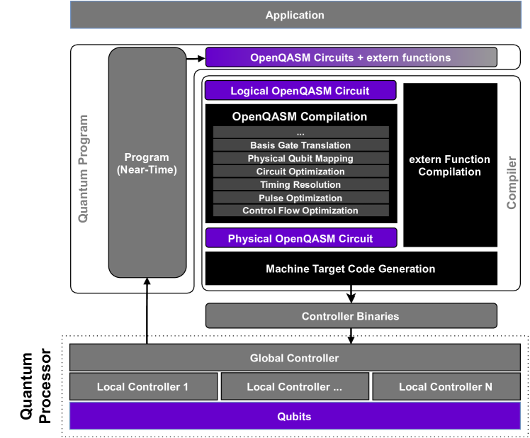
We illustrate a potential application compilation and execution flow for quantum programs in Figure 1. An application might be composed of several quantum programs including near-time calculations and quantum circuits. The quantum program interacts with quantum hardware by emitting OpenQASM3 circuits and external real-time functions. Initial generation of these circuits and extern} functions requires a deep compilation stack to transform the circuits and \qasmlineexterns into a form that is executable on the quantum processor (QPU). We represent these multiple stages by logical OpenQASM and physical OpenQASM. The logical OpenQASM represents the intent of the extended quantum circuit whereas the physical OpenQASM is the lowest level where the circuit is mapped and scheduled on specific qubits. A quantum program might work with even higher-level circuit representations than those expressible with OpenQASM 3, but in this flow, manipulations of these higher-order objects would be contained within the quantum program. A quantum program is not constrained to produce only logical OpenQASM. Sometimes it might emit physical OpenQASM, or later stages of a program might take advantage of lower-cost ways to produce binaries executable by the QPU. For instance, a program describing the optimization loop of a variational algorithm might directly manipulate a data section in the binaries to describe circuits with updated circuit parameters [Karalekas_2020]. We generically expect quantum programs to be able to enter the compilation toolchain at varying levels of abstraction as appropriate for different phases of program execution. Our language model further assumes that the QPU has a global controller that orchestrates execution of the circuit. This global controller centralizes control flow decisions and has the ability to execute extern} computations emitted by the quantum program. Some QPUs may also have a collection of local controllers that interact with a subset of qubits. Such segmentation of the QPU could enable concurrent execution of independent code segments.

3 Comparison to OpenQASM 2

OpenQASM 3 is designed to allow quantum circuits to be expressed in greater detail, and also in a more versatile way. However, we considered it important in extending this functionality to remain as close to the language structure of OpenQASM 2 as practically possible. Throughout this article, we occasionally note similarities or differences between OpenQASM versions 2 and 3. In this section, for the convenience of developers who are familiar with OpenQASM 2, we explicitly describe the OpenQASM 2 features which developers may rely on to work identically in OpenQASM 3.

Circuit header

Top-level circuits in OpenQASM 2 must begin with the statement “

OpenQASM 2.x;}’’,%
    \footnote

Throughout the rest of the article, to reduce clutter, we often omit terminal semicolons for in-line examples. possibly preceded by one or more blank lines or lines of comments, where x} is a minor version number (such as \qasmline0). Other source-files could be included using the syntax

include "filename"}, in the header or elsewhere in the circuit.
Top-level circuits in OpenQASM\,3 begin similarly, \emph

e.g., with a statement “OpenQASM 3.0}’’; and OpenQASM\,3 supports \qasmlineinclude statements in the same way.

Circuit execution

The top-level of an OpenQASM 2 circuit is given by a sequence of instructions at the top-level scope. No means of specifying an explicit entry point is provided: the circuit is interpreted as a stream of instructions, with execution starting from the first instruction after the header. A top-level OpenQASM 3 circuit may also be provided in this way: as a sequence of instructions at the top-level scope, without requiring an explicit entry point.

Quantum and classical registers

In OpenQASM 2, the only storage types available are qubits which are allocated as part of a qreg} declaration, and classical bits which are allocated as part of a \qasmlinecreg declaration, for example: qreg q[5]; // a register ’q’ with five qubits creg c[2]; // a register ’c’ with two classical bits This syntax is supported in OpenQASM 3, and is equivalent to the (preferred) syntax qubit[5] q; // a register ’q’ of five qubits bit[2] c; // a register ’c’ of two classical bits which respectively declares q} and \qasmlinec as registers of more primitive qubit} or \qasmlinebit storage types. (OpenQASM 3 also introduces other storage types for classical data: see Section 4.4.)

Names of gates, variables, and constants

In OpenQASM 2, the names of registers and gates must begin with a lower-case alphabetic ASCII character. This constraint is relaxed in OpenQASM 3: identifiers may now begin with other characters, such as capital letters, underscores, and a range of unicode characters. For example, angular values used as gate arguments may now be represented by greek letters. (The identifier π} is reserved in OpenQASM\,3 to represent the same constant as \qasmlinepi.) Note that OpenQASM 3 has a slightly different set of keywords from OpenQASM 2. This may cause errors in OpenQASM circuits which happen to use a keyword from version 3 as an identifier name: such identifiers would have to be renamed in order for the source to be valid OpenQASM 3.

Basic operations

In OpenQASM 2, there were four basic instructions which affected stored quantum data:

• Single-qubit unitaries specified with the syntax U(a,b,c)} for some angular parameters \qasmlinea

, b}, and \qasmlinec, acting on a single-qubit argument. This syntax is also supported in OpenQASM 3, and specifies an equivalent unitary transformation. Two-qubit controlled-NOT operations, using the keyword

CX}, acting on two single-qubit arguments.
    In OpenQASM\,3, the \qasmline

CX instruction is no longer a basic instruction or a keyword, but may be defined from more primitive commands. To adapt an OpenQASM 2 circuits to be valid OpenQASM 3, one may add a single instruction to define CX} using a ‘‘\qasmlinectrl @” gate modifier: gate CX c, t ctrl @ U(π,0,π) c, t A definition of this sort for CX} is also provided in the standard gate library for OpenQASM\,3, which we describe in Section~\refsec:std-gate-library. (The meaning of the “ctrl @}’’ gate modifier is described in Section~\refsec:ctrl-modifier.) Non-unitary reset} and \qasmlinemeasure operations, acting on a single-qubit argument (and producing a single bit outcome in the case of

measure}).
    The statement \qasmline

reset q[j] operation has the effect of discarding the data stored in q[j]}, replacing it with the state $\ket0$.Thestatement\verb{measure q[j] -> c[k]} has the effect of measuring \qasmline{q[j]$ in the standard basis, i.e., projecting the state into one of the eigenstates of the Pauli $Z$ operator, and storing the corresponding bit-value in a classical bit

c[k]}.
    OpenQASM\,3 supports these operations without changes, and also supports the alternative syntax \qasmline

c[k] = measure q[j] for measurements.

Gate declarations

OpenQASM 2 supports

gate} declarations to specify user-defined gates.
The definitions set out a fixed number of single-qubit arguments, and optionally some arguments which are taken to be angular parameters.
These declarations use syntax such as%
\begin

qasmblock gate h a U(π/2, 0, π) a; gate p(θ) a U(0, 0, θ) a; gate cp(θ) a, b p(θ/2) a; p(θ/2) b; CX a,b; p(-θ/2) b; CX a,b; The specification of these gates, in the code-blocks enclosed by braces { $\ldots$ }, are by sequences of unitary operations, whether basic unitary operations or ones defined by earlier

gate} declarations.
OpenQASM\,3 supports \qasmline

gate declarations with this syntax, and also admits only unitary operations as part of the gate definitions — but has greater versatility in how those unitary operations may be described (see Section 4.2), and also provides other ways to define subroutines (see Section 4.4).

Implicit iteration

Operations on one or more qubits could be repeated across entire registers as well, using implicit iteration. For instance, for any operation “’’ which acts on one qubit q[j]}, we can instead perform it independently on every qubit in \qasmlineq by omitting the index (as in “

qop q}’’).
For operations on two qubits of the form \mbox

“qop q[j], r[k]}’’}, one or both arguments could omit the index, in which case the instruction would be repeated either for $\textttj​=​1,2,…$or$k​=​1,2,…$(ifoneindexisomitted),orfor$j​=​k​=​1,2,…$(ifbothindicesareomitted).Thisfunctionalityalsoextendstooperationsonthreequbitsormore.OpenQASM\,3supportsthisfunctionalityunchanged,for\verb{gate} subroutines. (OpenQASM\,3 also supports other kinds of subroutine beyond \qasmline{gate$ definitions, and these other subroutines do not support implicit iteration in this way.)

Control flow

The only control flow supported by OpenQASM 2 are

if} statements.
These can be used to compare the value of a classical bit-register (interpreted as a little-endian representation of an integer) to an integer, and conditionally execute a single gate.
An example of such a statement is
\begin

qasmblock if (c == 5) mygate q, r, s; which would test whether a classical register c} (of length three or more) stores a bit-string $c_n-1 ⋯c_3 c_2 c_1 c_0$equalto$0 ⋯0101$,todeterminewhethertoexecute\verb{mygate q, r, s}. If-statements (and classical register comparisons) of this kind are supported in OpenQASM\,3, as is more general syntax for \qasmline{if$ statements and other forms of control-flow (see Section 4.4).

Barrier instructions

OpenQASM 2 provides a

barrier} instruction which may be invoked with or without arguments.
When invoked with arguments, either of individual qubits or whole quantum registers, it instructs the compiler not to perform any optimizations that involve moving or simplifying operations acting on those arguments, across the source line of the \qasmline

barrier statement; when invoked without arguments, it has the same effect as applying it to all of the quantum registers that have been defined. This operation is also supported in OpenQASM 3, with the same meaning.

Opaque definitions

OpenQASM 2 supports

opaque} declarations, to declare gates whose physical implementation may be possible but is not readily expressed in terms of unitary gates.
OpenQASM\,3 provides means of defining operations on a lower level than unitary gates (see Section~\ref

sec:calibrating), therefore opaque definitions are not needed. OpenQASM 3 compilers will simply ignore any

opaque} declarations.
\vspace*

-.5ex

Circuit output

The outputs of an OpenQASM 2 circuit are the values stored in any declared classical registers. OpenQASM 3 introduces a means of explicitly declaring which variables are to be produced as output or taken as input (see Section LABEL:sec:parameterised-circuits). However, any OpenQASM 3 circuit which does not specify either an output or input will, by default, also produce all of its classical stored variables (whether of type creg}, or a different type) as output.

4 Concepts of the language: the logical level

OpenQASM 3 is a multi-level IR for quantum computations, which expresses concepts at both a logical and a more fine-grained physical level. In this section we give a overview of the important features of the logical level of OpenQASM 3, presenting the more low-level features in Section LABEL:sec:physical-features. For a finer-grained specification, we direct readers to the live specification [livedoc].

4.1 Continuous gates and hierarchical library

We define a mechanism for parameterizing unitary matrices to define quantum gates. The parameterization uses a set of built-in single-qubit gates and a gate modifier to construct a controlled version to generate a universal gate set [barenco95]. Early QASM languages assumed a discrete set of quantum gates, but OpenQASM is flexible enough to describe universal computation with a continuous gate set. This gate set was chosen for the convenience of defining new quantum gates and is not an enforced compilation target. Instead of allowing the user to write a unitary as an $n\times n$ matrix, we make gate definitions through hierarchical composition allowing for code reuse to define more complex operations [scaffold, dousti16]. For many gates of practical interest, there is a circuit representation with a polynomial number of one- and two-qubit gates, giving a more compact representation than requiring the programmer to express the full $n\times n$ matrix. In the worst case, a general $n$-qubit gate can be defined using an exponential number of these gates. We now describe this built-in gate set. Single-qubit unitary gates are parameterized as

$$U(\theta,\phi,\lambda):=\left(\begin{array}[]{cc}\cos(\theta/2)&-e^{i\lambda}\sin(\theta/2)\\ e^{i\phi}\sin(\theta/2)&e^{i(\phi+\lambda)}\cos(\theta/2)\end{array}\right)$$ (1)

This expression specifies any element of $U(2)$ up to a global phase. The global phase is here chosen so that the upper left matrix element is real. For example,

U(π/2, 0, π) q[0];}
applies the Hadamard gate
$H = \frac

12 (1 -1 1 -1)$toqubit\verb{q[0]}. For the convenience of the reader, we note two important decompositions of $U$, through an Euler angle decomposition using rotations $R_z(\alpha) = \exp(-i\alpha Z/2)$ and $R_y(\beta) = \exp(-i\beta Y/2)$, and a $\{H,P\}$ basis representation where $P(\alpha)=\begin{pmatrix}1\,&\,0\\ 0\,&\,e^{i\alpha\!}\end{pmatrix}$:

$$U(\theta,\phi,\lambda)\;=\;e^{i(\phi+\lambda)/2}\,R_{z}(\phi)R_{y}(\theta)R_{z}(\lambda)\;=\;e^{i\theta/2}\,P(\phi\!+\!\pi/2)HP(\theta)HP(\lambda\!-\!\pi/2).$$ (2)

Note.  Users should be aware that the definition in Eq. 1 is scaled by a factor of $e^{i(\phi+\lambda)/2}$ when compared to the original definition in OpenQASM 2 [CBSG17]. This implies that the transformation described by  U(a,b,c)}\, has determinant $e^i(a+c)$,andisnotingeneralanelementof$SU(2)$.ThischangeinglobalphasehasnoobservableconsequenceforOpenQASM\,2circuits.Wealsonotethat\verb{U} is the only uppercase keyword in OpenQASM\,3. \smallskip \par New gates are associated to a unitary transformation by defining them using a sequence of built-in or previously defined gates and gate modifiers. For example, the \qasmline{gate$ declaration gate h q U(π/2, 0, π) q; defines a new gate called “h}’’ and associates it to the unitary matrix of the Hadamard gate. Once we have defined ‘‘\qasmlineh”, we can use it in later gate} blocks. The definition does not necessarily imply that \qasmlineh is implemented by an instruction U(π/2, 0, π)} on the quantum computer. The implementation is left to the user and/or compiler (see Section~\refsec:calibrating), given information about the instructions supported by a particular target. Controlled gates can be constructed by attaching a control modifier to an existing gate. For example, the NOT gate (i.e., the Pauli $X$ operator) is given by

U(π, 0, π)} and the block
\begin

qasmblock gate CX c, t ctrl @ U(π, 0, π) c, t; CX q[1], q[0]; defines the gate

$$\texttt{CX}:=I\oplus\texttt{x}=\left(\begin{array}[]{cccc}1&0&0&0\\ 0&1&0&0\\ 0&0&0&1\\ 0&0&1&0\end{array}\right)$$ (3)

and applies it to q[1]} and \qasmlineq[0]. This gate applies a bit-flip to q[0]} if \qasmlineq[1] is one, leaves q[1]} unchanged if \qasmlineq[0] is zero, and acts coherently over superpositions. The control modifier is described in more detail in Section 4.2. Remark.  Throughout the document we use a tensor order with higher index qubits on the left. This ordering labels states in a way that is consistent with how numbers are usually written with the most significant digit on the left. In this tensor order,

CX q[0], q[1];} is represented by the matrix
\begin

equation (1000000100100100). From a physical perspective, any unitary $U$ is indistinguishable from another unitary $\mathrm{e}^{i\gamma}U$ which only differs by a global phase. When we attach a control to these gates, however, the global phase becomes a relative phase that is applied when the control qubit is one. To capture the programmer’s intent, a built-in global phase gate allows the inclusion of arbitrary global phases on circuits. The instruction gphase(γ)} adds a global phase of $\mathrm e^iγ$tothescopecontainingtheinstruction.Forexample,\qasmblock gaterz(τ)q{gphase(-τ/2);U(0,0,τ)q;}ctrl@rz(π/2)q[1],q[0];constructsthegate\begin{equation}R_{z}(\tau)=\exp(-i\tau Z/2)=\begin{pmatrix}\mathrm{e}^{-i\tau/2}&0\\ 0&\mathrm{e}^{i\tau/2}\end{pmatrix}=\mathrm{e}^{-i\tau/2}\begin{pmatrix}1&0\\ 0&\mathrm{e}^{i\tau}\end{pmatrix}\end{equation}andappliesthecontrolledformofthatphaserotationgate\begin{equation}I\oplus R_{z}(\pi/2)=\begin{pmatrix}1&0&0&0\\ 0&1&0&0\\ 0&0&\!\mathrm{e}^{-i\pi/4}\!&0\\ 0&0&0&\!\mathrm{e}^{i\pi/4}\!\end{pmatrix}.\end{equation}\par InOpenQASM\,2,\verb{gate} subroutines are defined in terms of built-in gates \qasmline{U$ and CX}. In OpenQASM\,3, we can define controlled gates using the control modifier, so it is no longer necessary to include a built-in \qasmlineCX gate. For backwards compatibility, we include the gate

CX} in the standard gate library (described below), but it is no longer a keyword of the language.
\subsubsection

Standard gate library We define a standard library of OpenQASM 3 gates in a file we call stdgates.inc. Any OpenQASM 3 circuit that includes the standard library can make use of these gates. examples/stdgates.inc

4.2 Gate modifiers

We introduce a mechanism for modifying existing unitary gates g} to define new ones. A modifier defines a new unitary gate from \qasmlineg, acting on a space of equal or greater dimension, that can be applied as an instruction. We add modifiers for inverting, exponentiating, and controlling gates. This can be useful for programming convenience and readability, but more importantly it allows the language to capture gate semantics at a higher level which aids in compilation. For example, optimization opportunities that exist by analysing controlled unitaries may be exceedingly hard to discover once the controls are decomposed.

The control modifier

The modifier ctrl @ g} represents a controlled-\qasmlineg gate with one control qubit. This gate is defined on the tensor product of the control space and target space by the matrix ${{{{{{{I\oplus\texttt{\verb{}{}\@hidden@egroup gmissing{}{}\@hidden@egroup g}$\,,where$I$hasthesamedimensionsas\verb{g}. (We regard \qasmline{ctrl@gphase(a)} as a special case, which is defined to be the gate $1\oplus e^{i\;\!\mathtt{a}}=\text{\verb{}{}\@hidden@egroup U(0,0,a)missing{}{}\@hidden@egroup U(0,0,a)}$.)Acompilationtargetmayormaynotbeabletoexecutethecontrolledgatewithoutfurthercompilation.Theuserorcompilermayrewritethecontrolledgatetouseadditionalancillaryqubitstoreducethesizeanddepthoftheresultingcircuit.\par Forexample,wecandefinetheFredkin(orcontrolled-swap)gateintwodifferentways:\qasmblock//Someusefulreversiblegatesgatexq{U(π,0,π)q;}gatecxc,t{ctrl@xc,t;}gatetoffolic0,c1,t{ctrl@cxc0,c1,t;}gateswapa,b{cxa,b;cxb,a;cxa,b;}\par//Fredkindefinition#1gatefredkin1c,a,b{cxb,a;toffolic,a,b;cxb,a;}\par//Fredkindefinition#2gatefredkin2c,a,b{ctrl@swapc,a,b;}ThedefinitionsareequivalentbecausetheyresultinthesameunitarymatrixforbothFredkingates.Ifwedirectlyapplythedefinitions,\verb{fredkin1} involves fewer controlled operations than \qasmline{fredkin2}. A compiler pass may infer this fact or even rewrite \verb{fredkin2} into \qasmline{fredkin1}. Note that although the \verb{toffoli} gate is well defined here, the compiler or user needs to do further work to synthesize it in terms of more primitive operations, such as 1- and 2-qubit gates, or pulses (see Section~\ref{sec:calibrating}).\par Forasecondexample,ifwegoonestepfurther,wecandefineacontrolledFredkingate.Ifweusethe$ABA^\dagger$patterninthedefinitionofthe\verb{fredkin1} gate, we require only one controlled \qasmline{toffoli} gate after we remove unneeded controls from the \verb{cx} gates. Although the controlled \qasmline{toffoli} gate is defined on four qubits, it may be beneficial for a compiler or user to synthesize the gate using extra qubits as scratch space to reduce the total gate count or circuit depth, as in the following example: \qasmblock // Require: the scratch qubit is 'clean', i.e. initialized to zero // Ensure: the scratch qubit is returned 'clean' gate cfredkin2 c0, c1, a, b, scratch { cx b, a; // (from fredkin1) toffoli c0, c1, scratch; // implement ctrl @ toffoli c0, c1, a, b toffoli scratch, a, b; // by computing (and uncomputing) an AND of the two controls toffoli c0, c1, scratch; // in the scratch qubit cx b, a; // (from fredkin1) } \par We further provide the \verb{negctrl} modifier to control operations with \emph{negative}polarity,\emph{i.e.},\leavevmode\nobreak\ conditionedonthecontrolbitbeingzeroratherthanone.Both\verb{ctrl} and \qasmline{negctrl$ optionally accept an argument $n$ which specifies the number of controls of the appropriate type, which are added to the front of the list of arguments (omission means $n=1$). In each case, $n$ must be a positive integer expression which is a ‘compile-time constant’. For example, this can be useful in writing classical Boolean functions [schmitt2019scaling], as demonstrated by the following example (illustrated in Figure 2).

Figure 2: Toffoli network to compute a Boolean function $f=\bar{a}_{0}\bar{a}_{1}a_{2}a_{3}a_{4}\oplus\bar{a}_{0}a_{1}a_{2}\bar{a}_{3}\oplus\bar{a}_{0}a_{1}a_{3}a_{4}\oplus a_{0}\bar{a}_{1}a_{3}a_{4}\oplus a_{0}a_{1}a_{2}\oplus\bar{a}_{0}\bar{a}_{1}\bar{a}_{2}a_{3}$ in a target qubit. The control pattern may be expressed in OpenQASM via control gate modifiers.

examples/boolean.qasm

The inversion modifier

The modifier inv @ g} represents the inverse \qasmlineg^† of the gate

g}.
This can be easily computed from the definition of the gate \qasmline

g as follows.

• The inverse of any unitary operation $U=U_{m}U_{m-1}\dots U_{1}$ can be defined recursively by reversing the order of the gates in its definition and replacing each of those with their inverse $U^{\dagger}=U_{1}^{\dagger}U_{2}^{\dagger}\dots U_{m}^{\dagger}$.

• The inverse of a controlled operation $I\oplus U$ can be defined by reversing the operation which is controlled, as $(I\oplus U)^{\dagger}=I\oplus U^{\dagger}$ for any unitary $U$. That is, missing is defined to have the same meaning as missing (commuting the ‘’ modifier past the ‘’ modifier).

• The base case is given by replacing inv @ U(a, b, c)} by \qasmlineU(-a, -c, -b), and replacing inv @ gphase(a)} by \qasmlinegphase(-a). For example, gate rz(τ) q gphase(-τ/2); U(0, 0, τ) q; inv @ rz(π/2) q[0]; applies the gate inv @ rz(π/2)}, which is defined by \qasmline gphase(π/4); U(0,-π/2,0);  . For an additional example: the gate    would be rewritten as   , which is the same as  .

  The powering modifier

  The modifier pow(r) @ g} represents the $r$th power \qasmlineg^r of the gate

  g}, where $r$ is an integer or floating point number. Every unitary matrix $U$ has a unique principal logarithm $\log U = iH$, where $H$ has only real eigenvalues $E$ which satisfy $-\pi< E \leq \pi$. For any real $r$, we define the $r$th power as $U^r = \exp(i r H)$.
  For example, consider the Pauli $Z$ operator $\textrm

  z}} = \beginpsmallmatrix 1 & 0
  0 -1 $.Theprincipallogarithmis$log =\beginpsmallmatrix 0 & 0
  0 iπ $,fromwhichitfollowsthat\verb{z}$^{1/2$ = exp(12 log) = \beginpsmallmatrix 1 & 0
  0 i $.Inthisway,thedefinitions\qasmblock gatezq{U(0,0,π)q;}gatesq{pow(1/2)@zq;}allowustodefinethegate\verb{s} as the square root of \qasmline{z$. (A compiler pass is responsible for resolving $S$ into gates.) For another example, the principal logarithm of the Pauli $X$ operator ${\textrm{\verb{}{}\@hidden@egroup xmissing{}{}\@hidden@egroup x} = \begin{pmatrix}0 &1 \\ 1 &0\end{pmatrix}$is$\log{\verb{}{x}{}{x}=\tfrac}i\pi}{2}\begin{pmatrix}+1\,&\,-1\\ -1\,&\,+1\end{pmatrix}$. One can confirm that this operator has eigenvalues $0$ and $i\pi$, and ${\textrm{\verb{}{}\@hidden@egroup xmissing{}{}\@hidden@egroup x}^{1/2} := \exp(\tfrac{1}{2}\log{\verb{}{x}{}{x}) = \tfrac}1}{2}\begin{pmatrix}1{+}i\,&\,1{-}i\\ 1{-}i\,&\,1{+}i\end{pmatrix}$. Therefore the definitions of the $\sqrt{X}$ gate gate sx a gphase(π/4); U(π/2, -π/2, π/2) a; gate sx a pow(1/2) @ x a; are equivalent. In the case where $r$ is an integer, the $r$th power pow(r) @ g} can be implemented simply (albeit less efficiently) as $r$ repetitions of \qasmlineg when $r>0$, or $r$ repetitions of

  inv @ u} when $r<0$. Continuing our previous example,
  \begin

  qasmblock

pow(-2) @ s q[0]; defines and applies s}$^-2$.Thiscanbecompiledto\qasmblock inv@pow(2)@sq[0];andfurthersimplifiedinto\qasmblock inv@zq[0];withoutsolvingtheproblemofsynthesizing\verb{s}. In general, however, compiling \qasmline{pow(r)@g$ involves solving a circuit synthesis or optimization problem, even in the integral case.

4.3 Non-unitary operations

OpenQASM 3 includes two basic non-unitary operations, which are the same as those found in OpenQASM 2. The statement bit = measure q} measures a qubit \qasmlineq in the $Z$-basis, and assigns the measurement outcome, ‘0’ or ‘1’, to the target bit variable (see the subsection on classical types in Section 4.4). Measurement is ‘non-destructive’, in that it corresponds to a projection onto one of the eigenstates of $Z$; the qubit remains available afterwards for further quantum computation. The

measure} statement also works with an array of qubits, performing a measurement on each of them and storing the outcomes into an array of bits of the same length.
For example, the example below initializes, flips, and measures a register of 10 qubits.%
\begin

qasmblock qubit[10] qubits; bit[10] bits; reset qubits; x qubits; bits = measure qubits; For compatibility with OpenQASM 2, we also support the syntax measure q -> r} for a qubit \qasmlineq (or quantum register of some length $n$), and a bit variable

r} (or a classical bit register of the same length).
The statement \qasmline

reset q resets a qubit

q} to the state $|0\rangle$.
With idealised quantum hardware, this is equivalent to measuring \qasmline

q in the standard basis, performing a Pauli $X$ operation on the qubit if the outcome is ‘1’, and then discarding the measurement outcome. Mathematically, it corresponds to a partial trace over q} (\emphi.e., discarding it) before replacing it with a new qubit in the state $|0\rangle$. The reset} statement also works with an array of qubits, resetting them to the state $|0\rangle\otimes \cdots \otimes |0\rangle$.

4.4 Real-time classical computing

OpenQASM 2 primarily described static circuits in which the only mechanism for control flow were if} statements that controlled execution of a single \qasmlinegate. This constraint was largely imposed by corresponding limitations in control hardware. Dynamic circuits — with classical control flow and concurrent classical computation — represent a richer model of computation, which includes features that are necessary for eventual fault-tolerant quantum computers that must interact with real-time decoding logic. In the near term, these circuits also allow for experimentation with qubit re-use, teleportation, and iterative algorithms. Dynamic circuits have motivated significant advances in control hardware capable of moving and acting upon real-time values [Ryan2017, Fu2017, Butko2019]. To take advantage of these advances in control, we extend OpenQASM with classical data types, arithmetic and logical instructions to manipulate the data, and control flow keywords. While our approach to selecting classical instructions was conservative, these extensions make OpenQASM Turing-complete for classical computations in principle, augmenting the prior capability to describe static circuits composed of unitary gates and measurement.

Classical types:

In considering what classical instructions to add, we felt it important to be able to describe arithmetic associated with looping constructs and the bit manipulations necessary to shuttle data back and forth between qubit measurements and other classical registers. As a result, simple classical computations can be directly embedded within an OpenQASM 3 circuit. To support these, we introduce classical data types like signed/unsigned integers and floating point values, to provide well-defined semantics for arithmetic operations. The OpenQASM type system was designed with two distinct requirements in mind. When used within high-level logical OpenQASM circuits the type system must capture the programmer’s intent. It must also remain portable to different kinds of quantum computer controllers. When used within low-level physical OpenQASM circuits the type system must reflect the realities of particular controller, such as limited memory and well-defined register lengths. OpenQASM takes inspiration from type systems within classical programming languages but adds some unique features for dynamic quantum circuits. For logical-level OpenQASM circuits, we introduce some common types which will be familiar to most programmers:

int} for signed integers,
\qasmline

uint