Chromospheric Activity in 55 Cancri:
II. Theoretical Wave Studies versus Observations

Abstract

In this study, we consider chromospheric heating models for 55 Cancri in conjunction with observations. The theoretical models, previously discussed in Paper I, are self-consistent, nonlinear and time-dependent ab-initio computations encompassing the generation, propagation, and dissipation of waves. Our focus is the consideration of both acoustic waves and longitudinal flux tube waves amounting to two-component chromosphere models. 55 Cancri, a K-type orange dwarf, is a star of low activity, as expected by its age, which also implies a relatively small magnetic filling factor. The Ca II K fluxes are computed (multi-ray treatment) assuming partial redistribution and time-dependent ionization. The theoretical Ca II H+K fluxes are subsequently compared with observations. It is found that for stages of lowest chromospheric activity the observed Ca II fluxes are akin, though not identical, to those obtained by acoustic heating, but agreement can be obtained if low levels of magnetic heating — consistent with the assumed photospheric magnetic filling factor — are considered as an additional component; this idea is in alignment with previous proposals conveyed in the literature.

1 Introduction

This study is a continuation of our previous work aimed at describing chromospheric heating in late-type stars by considering both theoretical wave models and observations. A large body of previous work, see, e.g., Schrijver & Zwaan (2000) and references therein, indicates that the atmospheres of highly active stars are dominantly heated by magnetic processes, including magnetic waves (e.g., Shoda et al., 2020), whereas for the atmospheric heating of low-activity stars non-magnetic processes are expected to play a more prominent role (e.g., Schrijver, 1995; Buchholz et al., 1998; Cuntz et al., 1999), even though magnetic phenomena. When stars age, the relative importance of atmospheric magnetic processes tends to subside, a process closely related to the evolution of angular momentum (e.g., Keppens et al., 1995; Charbonneau et al., 1997; Wolff & Simon, 1997; Matt et al., 2015; Mittag et al., 2018).

Here we focus on 55 Cancri (55 Cnc, $\rho^{1}$ Cnc), a G8 V star (Gonzalez, 1998) of advanced age, also identified as an orange dwarf. Orange dwarfs are of particular interest to a large range of astrophysical studies as, for example, they constitute transitory objects regarding various kinds of atmospheric heating processes. 55 Cnc is an example of a slow rotating star as its slow rotation is closely connected to its advanced age; see, e.g., Skumanich (1972) and subsequent work, including Barnes (2003, 2007), for background information. Following Fawzy & Cuntz (2021), see Paper I, this information is relevant for constraining the stellar photospheric and chromospheric magnetic filling factor (MFF), in part based on empirically deduced statistical relationships (e.g., Cuntz et al., 1999, and references therein). Additionally, information on the magnetic and nonmagnetic heating parameters has been provided as well.

Orange dwarfs are of particular interest to both astrophysics and astrobiology in consideration of various features, including those commonly considered favorable in support of exolife (e.g., Cuntz & Guinan, 2016; Lingam & Loeb, 2018, 2019; Dvorak et al., 2020). Those include the relative frequency of those stars (if compared to stars akin to the Sun), the relatively large size of their habitable zones (HZs) (if compared to M dwarfs), and their long main-sequence life times (i.e., 15 Gyr to 30 Gyr, compared to about 10 Gyr for solar-like stars; see, e.g., Pols et al. 1998). Recent work on the significance of late G and K dwarfs for the possibility of supporting exolife has been given by, e.g., Arney (2019) and Schulze-Makuch et al. (2020).

Previous studies about 55 Cnc also entertain the possible existence of Earth-type planets as part of the 55 Cnc system, especially in the region between 0.8 au and 5.7 au from the star. This spatial domain allows terrestrial planets to exhibit long-term orbital stability (e.g., Raymond et al., 2008; Satyal & Cuntz, 2019). Another pivotal motivation for the study of outer atmospheric heating and emission in 55 Cnc and similar stars is set by the emergent field of space weather simulations. This kind of work helps to augment our understanding of stellar and planetary environments, besides fostering basic astrophysical research (e.g., Lammer et al., 2012; Airapetian et al., 2020).

Our paper is structured as follows: In Section 2, we convey our theoretical approach, including comments on the time-dependent wave computations. In Section 3, we discuss observational aspects, including the calibration of the observed spectrum. Results and discussions are given in Section 4, including a discourse on the comparison between the theoretical models and observations. In Section 5, we report our summary and conclusions.

2 Theoretical Approach

2.1 Stellar Parameters

We pursue atmospheric studies of 55 Cnc, a G8 V star (Gonzalez, 1998) that has a mass of about 0.91 $M_{\odot}$ (von Braun et al., 2011). Its effective temperature has been determined as $5165{\pm}46$ K (Ligi et al., 2016) and $5172{\pm}18$ K (Yee et al., 2017). Furthermore, 55 Cnc is notably older than the Sun with previous estimates given as 8.6 Gyr (Mamajek & Hillenbrand, 2008) and 10.2 Gyr (von Braun et al., 2011); see also Bourrier et al. (2018) for discussion. Previous work about 55 Cnc’s rotation period indicates values of 42.2 d (Henry et al., 2000) and 38.8 d (Bourrier et al., 2018); clearly, these values of slow rotation are closely connected to 55 Cnc’s age, see, e.g., Skumanich (1972) and subsequent work. As pointed out in Paper I, the stellar rotation period also allows default estimates of the stellar photospheric magnetic filling factor (see Figure 1).

In the context of chromospheric heating, increased amounts of magnetic heating (in a statistical sense) are strongly correlated with increased outer atmospheric emission (e.g., Linsky, 1983), and related studies. Moreover, as discussed by Cuntz et al. (1998, 1999) and references therein, it is also possible to link $B_{0}f_{0}$ to both the stellar rotation period $P_{\rm rot}$ (e.g., Marcy & Basri, 1989; Montesinos & Jordan, 1993; Saar, 1996a; Reiners et al., 2009) as well as to the emergent chromospheric emission flux (e.g., Saar & Schrijver, 1987; Schrijver et al., 1989; Montesinos & Jordan, 1993; Saar, 1996b; Jordan, 1997). Related theoretical studies for sets of main-sequence stars, including objects akin to 55 Cnc, have been given by Fawzy et al. (1998, 2002b).

An important aspect concerning the magnitude of stellar activity, as given by the Ca II emission, pertains to the Rossby number (i.e., the ratio between the stellar rotational period and the local convective turnover time, $\tau_{\rm c}$). The Rossby number is related to the dynamo process; it also exhibits an observational correlation with the stellar activity. Based on work by, e.g., Montesinos et al. (2001), Cranmer & Saar (2011), and Castro et al. (2014), $\tau_{\rm c}$ for 55 Cnc is given as about 21.5 d; thus, the Rossby number for 55 Cnc is identified as ${\rm Ro}\simeq 1.9$, consistent with a star of low chromospheric activity; see Appendix A for details. Noyes et al. (1984) previously identified correlations between $P_{\rm rot}$ and the chromospheric basal flux emission, showing well-pronounced trends albeit considerable scatter with respect to the observational data.

Empirically, the decrease of activity in main-sequence stars does not necessarily concur with their absolute age, but rather with their relative main-sequence age as the magnetic braking time-scale increases downward on the main-sequence akin to their main-sequence evolutionary life time (Reiners & Mohanty, 2012; Schröder et al., 2013). But 55 Cnc is more evolved than the Sun even on a relative time-scale, in consideration of that 55 Cnc has passed about 2/3 of its time on the main-sequence (which is about 15 Gyr), contrary to the Sun with an age of about mid main-sequence. Hence, 55 Cnc is indeed a low-activity star while being quite evolved.

2.2 Time-dependent Wave Calculations

In Paper I, we pursued theoretical wave calculations based on acoustic waves (ACWs) and longitudinal flux tube waves (LTWs). Previously developed codes allowed us addressing the different steps of the magneto-acoustic heating picture, comprised of convective energy generation (e.g., Musielak et al., 1994, 1995; Ulmschneider et al., 1996), the propagation and dissipation of waves through different layers of the stellar atmosphere (e.g., Buchholz et al., 1998; Fawzy et al., 2002a), and the emergence of radiative energy output (e.g., Cuntz et al., 1999; Fawzy et al., 2002a). Both acoustic and magnetic waves are followed starting from the stellar convective zone to the point of shock formation and beyond. As discussed in Paper I, the initial wave energy fluxes for ACWs and LTWs have been chosen as $F_{\rm ACW}=3.3\times 10^{7}$ erg cm^-2 s^-1 and $F_{\rm LTW}=1.7\times 10^{8}$ erg cm^-2 s^-1, respectively. We examined models based on monochromatic waves and frequency spectra. In case of monochromatic waves, we chose $P=60$ s as representative period. This value is motivated by the shapes of the ACW and LTW frequency spectra as in both spectra the wave energy flux reaches its maximum close to that value (see Paper I).

The photospheric MFF is set by an empirical relationship based on observed values for the stellar rotation period, $P_{\rm rot}$; see Cuntz et al. (1999). Assuming 42.2 d (Henry et al., 2000) and 38.8 d (Bourrier et al., 2018) amount to $f_{0}=0.3$% and $1.4$%, respectively. The adopted MFF also informs the shape of the magnetic flux tubes as considered for our studies (see Fig. 1). The chromospheric Ca II fluxes are computed by considering non-local thermodynamic equilibrium (NLTE) and partial redistribution (PRD). In addition, effects originating from time-dependent ionization (TDI) have been taken into account as well; see Rammacher & Ulmschneider (2003) and Fawzy et al. (2012) for details. The self-consistent treatment of TDI (especially for hydrogen) greatly impacts the atmospheric temperatures and electron densities (especially behind the shocks); it also affects the emergent Ca II fluxes. See Fig. 2 for an example of a snapshot series pertaining to the dynamics associated with LTW spectral waves, including information on the Ca II/Ca and Mg II/Mg ionization degrees.

For the adequate representation of the multi-level atomic model for Ca II, we rely on previous results by Fawzy (2015). In order to model the total radiative energy losses, adequate scaling factors are applied to both the Ca II K and Mg II k lines. Radiative energy fluxes for our two-component chromosphere models, based on both ACWs and LTWs, are computed through implementing multi-ray treatments. For selected sets of models, increased initial wave energy fluxes are used to mimic the impact of torsional flux tube waves (TTWs) regarding the wave energy budget as expected through the occurrence of mode coupling (e.g., Hollweg et al., 1982; Kudoh & Shibata, 1999; Bogdan et al., 2003; Hasan et al., 2003).

Table 1: Summary of Acronyms

Acronym	Definition
ACW	Acoustic Wave
HZ	Habitable Zone
LTE	Local Thermodynamic Equilibrium
LTW	Longitudinal Flux Tube Wave
MFF	Magnetic Filling Factor ($f_{0}$)
NLTE	Non-Local Thermodynamic Equilibrium
NTDI	Non-Time-Dependent Ionization
PRD	Partial Redistribution
TDI	Time-Dependent Ionization
TTW	Torsional Flux Tube Wave

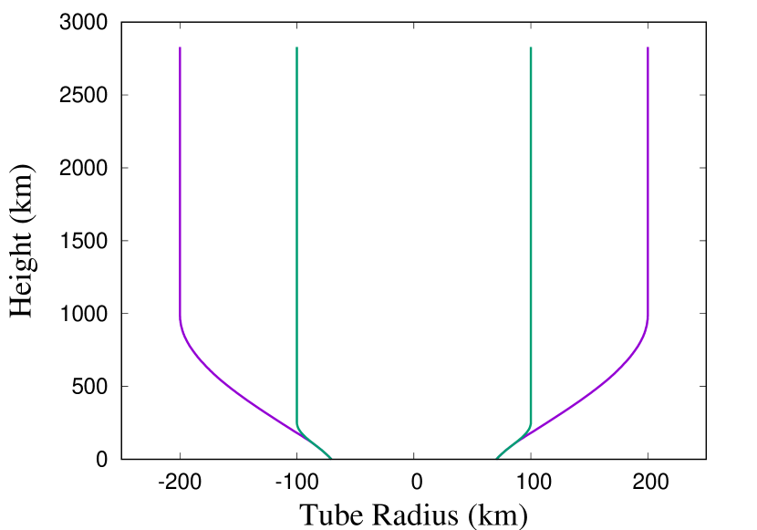
Figure 1: Initial magnetic flux tube models for 55 Cnc. The photospheric magnetic filling factor (main models) is given as $f_{0}$ = 0.3% (purple). We also discuss some models with $f_{0}$ = 1.4% for comparison (green). The tube opening radii are given as 100 km and 200 km, respectively; see Paper I for further information.

Table 2: Results for the LTW TDI Mechanical Energy Flux

Height	LTW		2 $\times$ LTW
…	$f_{0}=0.3$%	$1.4$%	$0.3$%	$1.4$%
(km)	(cgs)	(cgs)	(cgs)	(cgs)
Monochromatic Wave Models
0	8.23	8.23	8.53	8.53
250	7.60	7.64	7.85	7.89
500	7.24	7.52	7.45	7.72
750	6.81	7.10	6.96	7.26
1000	6.22	6.49	6.36	6.63
1250	5.57	5.80	5.70	5.94
1500	4.92	5.12	5.04	5.25
1750	4.35	4.49	4.44	4.61
2000	3.84	3.94	3.92	4.05
2250	3.38	3.49	3.46	3.59
2500	2.96	3.09	3.05	3.23
Spectral Wave Models
0	8.23	8.23	8.53	8.53
250	7.58	7.56	7.84	7.83
500	7.18	7.47	7.40	7.67
750	6.78	7.16	7.02	7.35
1000	6.34	6.68	6.56	6.87
1250	5.84	6.16	6.03	6.33
1500	5.26	5.57	5.40	5.77
1750	4.77	5.03	4.81	5.18
2000	4.28	4.52	4.32	4.64
2250	3.84	4.04	3.87	4.12
2500	3.41	3.55	3.47	3.58
Note: Results are given in logarithmic units.

3 Observational Aspects

3.1 Background Information

A major factor in the comparison of the theoretical Ca II K line profile and the total Ca II K emission with observations, besides considering the instrumental profile, is given by the photon absorption and reemission processes. The latter occur between the bottom of chromosphere, where the emission is produced, and the top, where the observed line profile emerges. In the absence of considerable collisions ($C\ll A$ for the Ca II H+K transition), owing to the relatively low chromospheric densities, absorbed photons are almost always reemitted. Hence, we can expect not to lose any of the produced emission, and even though the chromosphere is optically thick, it is nonetheless “effectively optically thin”. Thus, the computed emission measure should directly reflect the observed value.

However, the many absorption and reemission processes in the Ca II H and K lines, along the line of sight in consideration of the chromospheric mass column density, amount to the well-known Wilson-Bappu effect (Wilson & Bappu, 1957), which in the example studied here operates in a single chromosphere. As previously described by Ayres et al. (1975), during that process the photons migrate toward the wings of the line profile, where their escape probability is larger as the optical depth there is smaller. Consequently, a line broadening effect occurs, caused by the high optical depth at the centers of the Ca II H and K lines that depends on the mass column density of the particular chromosphere. Consequently, the widening effect is larger for stars of lower gravity, notably for giant stars. More luminous giants have a lower gravity, a larger chromospheric scale height, and, consequently, exhibit broader Ca II H and K emission lines.

The Wilson-Bappu effect can usually only be observed by comparing stars of different surface gravity. Here, however, we have the unique opportunity of discerning this widening process for a given chromosphere, as we are able to compare the computed line profile produced at the bottom with the one at the top, noting that the latter given as the observed emergent line profile.

3.2 Comparing Initial and Emerging Emission Line Profiles: The Wilson-Bappu Effect at Work

The main focus of this study is to compare the Ca II K emission line profile, generated due to wave heating (see Paper I) and mostly formed at the bottom of the chromosphere near the temperature minimum, with observations. The observed line spectrum (resolving power: $R$=115.000) was obtained in 2013 (Ridden-Harper et al., 2016) at HARPS-N. The associated instrumental line profile has a width of only 0.035 Å, which is more than an order of magnitude narrower than the intrinsic line width.

The observed emission line profile is, in fact, noticeably wider than that of the theoretically expected emission, i.e., $W_{\circ}=0.50$ Å compared to, typically, $W_{\circ}=0.25$ Å at half peak (based on the description by O. C. Wilson). At the base of the emission, the difference is 0.70 Å, as of the observed profile, compared to 0.50 Å for the computed emission profiles; see Fig. 3 for a direct comparison. Surely, the observed profile is also embedded in the relatively wide photospheric core of that line. Its residual flux is defined by the temperature of the stellar atmosphere at and below the temperature minimum region.

Hence, this difference in the emission line width being much too large to be attributable to instrumental effects, it is apparent that the line profile is mostly due to the Wilson-Bappu effect operating along the line of sight. In particular, the many absorption and reemission processes each emerging photon undergoes favors the migration into the wings of the line profile function, resulting in the broadening of the line (see Sect. 3.1) The explanation of this process, as forwarded by Ayres et al. (1975), suggests a distinct relationship between the mass column density $N$ and gravity $g_{\star}$ ($N\propto 1/\sqrt{g_{\star}}$). Thus, it yields a dependence of the line width $W_{\circ}$ to the star’s gravity given as $W_{\circ}\propto{g_{\star}}^{-0.25}$. A comparison of giant stars of known physical parameters indicates that this assessment is largely consistent with observation; see, e.g., Ayres et al. (1975), Lutz & Pagel (1982), and work in progress by one of us (K.-P. S.).

In this paper, however, we are able to demonstrate that this effect also operates in a distinct chromosphere, as we can showcase the comparison of the observed chromospheric emission line profile with the one obtained by theoretical modelling. This unique opportunity allows us, from a different point of view, to highlight density broadening as the best explanation for the Wilson-Bappu effect — considering that previously an alternative explanation for the line width, based on Doppler broadening by turbulence, has been forwarded; see, e.g., Reimers (1973) as well as the extensive discussion by Lutz & Pagel (1982). So far, this alternate explanation of the emission line broadening has never been fully ruled out.

In fact, the Wilson-Bappu effect, if operating as discussed, is also producing the right magnitude of line broadening. To demonstrate this, we may simply compare a hypothetical star of twice the chromospheric column density as 55 Cnc, by having only a quarter of its gravity, but otherwise having the same effective temperature and metallicity. Hence, its Ca II line emission width $W_{\circ}$ is increased by a factor of $g_{\star}^{-0.25}\propto\sqrt{2}$. Considering an instrumental profile width of 35 mÅ, the true value of 55 Cnc’s emission line width $W_{\circ}$ is expected to be close to 465 mÅ, or by 215 mÅ larger than the theoretical emission line width at the bottom of 55 Cnc’s chromosphere, whereas $W_{\circ}$ of the hypothetical star would amount to 660 mÅ. In other words, adding the same chromospheric column density once again in this application, the Wilson-Bappu effect entails an additional line broadening by the same amount (i.e., about 200 mÅ) as the one required to reconcile the theoretically predicted emission line width with the observed one considering the radiative transfer regarding 55 Cnc’s chromosphere (see Fig. 3).

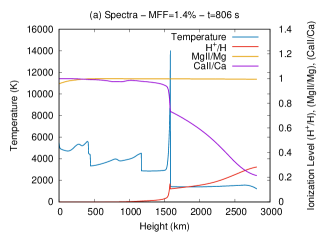
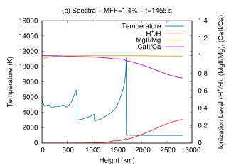
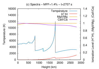
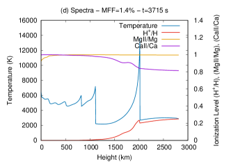
Figure 2: Snapshot series for a LTW TDI model based on spectral waves and a MFF of $f_{0}=1.4$%.

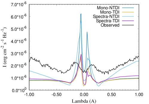
Figure 3: Examples of Ca II K profiles for LTWs based on $f_{0}=0.3$% in comparison with observations.

3.3 On the Flux Scale of the Observed Spectrum

In order to calibrate the scale of the normalized spectral flux of the observed Ca II K line profile with respect to the spectral surface flux in absolute terms, we used the best-matching spectrum based on the PHOENIX atmospheric model based on the parameters for 55 Cnc given as $T_{\rm eff}=5200$ K, $\log{g_{\star}}=4.0$ (cgs), and [Fe/H]=0.5, which are consistent with the observed values. The spectrum as obtained fits well the relatively wide photospheric Ca II K profile, contrary to, e.g., the model based on $T_{\rm eff}=5100$ K previously used in the literature.

Note that the latter value results in a much wider photospheric Ca II K line profile. This difference is relevant for the calibration process as that cooler model already implies a 20% lower near-UV spectral flux. Since the photospheric wings are a very sensitive indicator of the stellar effective temperature, we therefore opt in favor of the former value. In fact, $T_{\rm eff}$ seems to lie somewhere between 5100 K and 5200 K. Additionally, the limited resolution of the model library regarding [Fe/H] and $\log{g_{\star}}$ made us choose a slightly higher value for [Fe/H] and a slightly lower value for $\log{g_{\star}}$ than observed. Ultimately, effects on the synthetic spectrum based on these small parameter deviations largely cancel each other out.

In particular, we hinged the spectral surface flux scale calibration on line-free points in the Ca II K photospheric profile, from about 2 Å away of the very core outwards. Of particular use here is the region around $-2.5$ Å, which is sufficiently far away from the somewhat mismatched innermost photospheric line core. Note that this process is based on the standard 1-D, NLTE, and photosphere-only models. They do not account for the stellar chromosphere entailing that the temperature minimum is artificially low. On the other hand, only the innermost photospheric Ca II H+K line cores are formed at those outermost photospheric layers. Therefore, the rest of the PHOENIX Ca II K line profile matches the observed spectrum very well.

Matching the normalized observed flux scale to the above-mentioned PHOENIX spectrum including its spectral surface flux scale results in a factor of $1.75\times 10^{-5}$; this factor is needed for multiplying the observed normalized flux to arrive at physical flux units. It also considers the different units used by the PHOENIX spectra (i.e., spectral flux per wavelength in cm), while we use a spectral flux per frequency in Hz.

Figure 3 conveys the obtained direct and quantitative comparison of the observed and computed chromospheric emission on the spectral surface flux scale. We estimate the residual uncertainty of the scaling to be on the order of 20% based on the expected impact of a small (by 100 K) mismatch of $T_{\rm eff}$. Moreover, the observed emission rises from the deep photospheric line core, rather than from flat zero, and it is widened by the above described Wilson-Bappu effect, i.e., the migration of the photons into the wings of the line profile function by line saturation effects due to the relatively large Ca II mass column density. Nonetheless, the emission measures — to be visualized as the area of the emission line profile — are in good agreement.

4 Results and Discussion

4.1 Time-dependent Two-Component Heating Models

Time-dependent two-component heating models, based on ACWs and LTWs, have been obtained in Paper I. These models are used to calculate the emergent Ca II H+K fluxes in correspondence to the various theoretical models. The most relevant results obtained in Paper I include that both ACWs and LTWs form shocks in the upper photosphere / lower chromosphere. Regarding monochromatic waves, the height of shock formation for LTWs (with $f_{0}=0.3$%) was identified as about 30 km lower than in ACWs due to the higher wave energy flux. Generally, higher shock strengths are attained for spectral waves compared to monochromatic waves. Notable differences between the models occur at larger heights, mostly due the dilution of the wave energy flux.

In the present study, we revisited this aspect by comparing wave models of different MFFs and initials wave energy fluxes, given as $F_{\rm LTW}$ and $2\times F_{\rm LTW}$; we also assumed TDI (see Table 2). We found that the wave energy fluxes decreased by many orders of magnitude as a function of height, as expected. For a fixed height, a larger MFF resulted in a higher value for the wave energy flux, a consequence of the different magnitude of wave energy flux dilution (see Fig. 1). For example, at heights of 750 km, the difference between $f_{0}$ = 0.3% and 1.4% resulted in a factor between 2.0 and 2.4 regarding $F_{\rm LTW}$, depending on the model, whereas at 1500 km, that factor varied from 1.6 to 2.3. Different initial wave energy fluxes were most consequential in the low and mid chromosphere, with the difference starting to fade with increasing atmospheric height, as expected based on the limiting shock strength behavior (Cuntz, 2004). Spectral waves entail a somewhat larger wave energy flux at large heights as those models exhibit a smaller spatial decrease of the atmospheric density.

The formation heights for Ca II and Mg II range were found to be between 700 km and 1800 km, depending on the model. Radiative energy losses were identified to be most pronounced behind strong shocks owing to the impact of shock-shock interaction and in models with time-dependent hydrogen ionization omitted; i.e., models based on non-fully time-dependent ionization (NTDI). Shock-shock interaction entails the merging of shocks, which leads to the formation of shocks of large strengths. They result in strong heating events as well as significant large-scale cooling due to momentum transfer (e.g., Cuntz, 1987; Carlsson & Stein, 1992).

Peaks of Ca II and Mg II emission behind shocks (including those of large strengths) are absent in TDI models owing to the difference in the time-scales between the ionization processes and shock propagation. Additionally, the mean atmospheric temperatures were found to be highest in monochromatic wave models compared to spectral wave models; this is a consequence of quasi-adiabatic cooling owing to the momentum transfer by strong shocks. This result agrees well with previous work by, e.g., Carlsson & Stein (1992, 1995, 2002), on wave simulations for the Sun.

Figure 2 depicts a snapshot series for a LTW TDI model based assuming spectral waves with an initial energy flux of $F_{\rm LTW}=1.7\times 10^{8}$ erg cm^-2 s^-1 (see Sect. 2.2). Each figure panel features a dominant shock formed by shock merging. This process can be examined based on the time-dependent and height-dependent development of individual shocks. For example, shock number 37, inserted at an elapsed time of 1500 s, shows an increase in strength $M_{\rm sh}$ given as 1.23, 4.32, and 6.15 at elapsed times of 1550 s, 1600 s, and 1650 s, respectively. The relative density jumps $\eta$ across the shocks are identified as 0.34, 2.44, and 2.71.

It is also found that Mg is completely ionized to Mg II, except in parts of the stellar photosphere. However, the Ca II/Ca ionization degree decreases from 100% (mid chromosphere) to notably lower values at larger heights. At 2000 km, for the time-steps depicted in Fig. 2, we find values between 60% and 95% due to the ionization of Ca II to Ca III. However, there is no noticeable change in Ca and Mg ionization degrees between the pre-shock and post-shock regions owing to the non-instantaneous nature of ionization; see, e.g., Kneer (1980) and subsequent studies for detailed information.

4.2 Comparisons with Observations

A key aspect of this study is the comparison between the results of our theoretical models, based on both ACWs and LTWs, and observations. Table 3 summarizes the results obtained for the Ca II H+K fluxes from the various models and the observations (see Appendix A for details). The prime observational value is given as log $F_{\rm Ca~{}II~{}H+K}$ = 5.835, corresponding to the approximate chromospheric minimum value without the photospheric contribution. Although our theoretical models only provide the Ca II K fluxes, we use the conversion $R_{\rm K}/R_{\rm H}=1.04$ amounting to $R_{\rm K}+R_{\rm H}/R_{\rm K}=1.96$. This formula utilizes previous theoretical work by Cuntz et al. (1999) and references therein indicating the $R_{\rm K}/R_{\rm H}$ is highest for stars of largest chromospheric activity, corresponding to fasted rotation, i.e., lowest value of $P_{\rm rot}$. Table 3 conveys that LTW models based on $f_{0}$ = 0.3% appear to be most consistent with the observed Ca II H+K fluxes.

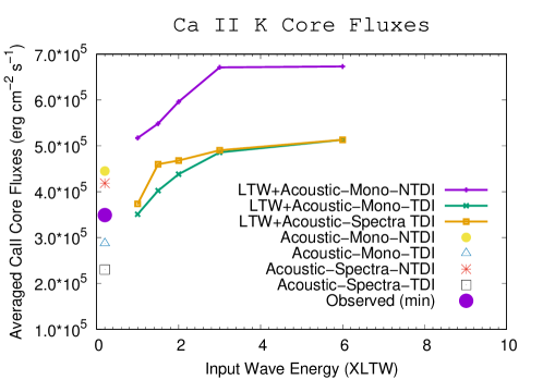
Figure 4: Averaged Ca II K core fluxes for different types of models as a function of multiples of LTW wave energies based on $f_{0}$ = 0.3%. Results are given for monochromatic NTDI and TDI models, as well as spectral TDI models. Moreover, we also give the results for the various models based on acoustic waves as well as the result from observations (approximate minimum value).

Table 3: Comparison of Ca II H+K Fluxes

Model	MFF	Description	Result
Acoustic	…	Mono-TDI	5.75
…	…	Spectra-TDI	5.65
1.0 LTW	$0.3\%$	Mono-TDI	5.84
…	$0.3\%$	Spectra-TDI	5.86
1.0 LTW	$1.4\%$	Mono-TDI	6.05
…	$1.4\%$	Spectra-TDI	6.11
2.0 LTW	$0.3\%$	Mono-TDI	5.93
…	$0.3\%$	Spectra-TDI	5.96
3.0 LTW	$0.3\%$	Mono-TDI	5.98
…	$0.3\%$	Spectra-TDI	5.98
Observed (min, approx.)	…	…	5.835
Note: The results are given in logarithmic units.

Figure 4 displays the Ca II K core fluxes (defined over a wavelength range of $\Delta\lambda=\pm 0.3$ Å) for different types of models together with the observed value. It shows again that the two-component chromosphere model (ACW + LTW) with $f_{0}=0.3$% is most consistent with the observations. Models based on pure acoustic waves yield Ca II K core fluxes that are notably too small. This figure also shows that Ca II K core fluxes based on models with TTWs (see Paper I for details), according to the approximation as used here, are considerably too high in order to successfully describe the observed minimal Ca II chromospheric emission. The models exhibit a notably increased mechanical energy flux in the Ca II line formation region accounting for the difference (see Table 2). However, these models are expected to be relevant for stages of higher activity as previously also obtained for 55 Cnc.

5 Summary and Conclusions

We pursued various chromospheric heating calculations for 55 Cnc, a main-sequence star of spectral-type late-G taking into account that this star generally exhibits a low level of chromospheric activity. According to previous work by, e.g., Linsky (1983) and others, magnetic heating in stellar atmospheres is strongly correlated to increased outer atmospheric emission. For 55 Cnc, the magnitude of magnetic heating is expected to be relatively low. This behavior stems from its old age (Mamajek & Hillenbrand, 2008; von Braun et al., 2011; Yee et al., 2017) and slow rotation (Henry et al., 2000; Bourrier et al., 2018). Stellar evolution models indicate that late-type main-sequence stars gradually lose angular momentum resulting in a steady decrease of stellar activity (e.g., Charbonneau et al., 1997; Mittag et al., 2018).

Our set of theoretical models is based on detailed studies of ACWs and LTWs. Both kinds of waves form shocks leading to modified thermodynamic atmospheric structures and emergent Ca II H+K and Mg II h+k emission line fluxes. Using Ca II K as an appropriate representation of the overall chromospheric emission flux, the line has been calculated in detail (multi-ray treatment) assuming PRD in combination with TDI (main models). Furthermore, our study makes use of previous work by Musielak et al. (1994, 1995); Ulmschneider et al. (1996), and Fawzy & Cuntz (2011) that provides detailed information on the amounts of magneto-acoustic heating based the adopted stellar parameters. In addition, 55 Cnc’s photospheric MFF has been estimated to be relatively low; therefore, we calculated sets of models based on $f_{0}$ = 0.3% and 1.4%.

As expected, models of different MFFs indicate that larger MFFs correspond to higher (on average) chromospheric temperatures. Those models also show higher Ca II and Mg II emissions as well as higher Ca and Mg ionization rates, especially in the upper magnetically heated chromospheres (see Paper I for details). Additionally, different MFFs result in different rates of dilution of the magnetic wave energy fluxes, which are instrumental for the energetics mirrored by both the shock dissipation and the emergent radiative emission at different atmospheric heights.

Comparisons with observations indicate that considering 55 Cnc’s low activity stage, the emergent Ca II flux can best be reproduced by a combination of acoustic heating and longitudinal flux tube heating, as stipulated by a small photospheric magnetic filling factor informed by the star’s slow rotation rate. Based on our master models, assuming both time-dependent ionization and spectral waves, a MFF of $f_{0}$ = 0.3% appears to be more consistent with the Ca II observations than $f_{0}$ = 1.4%. The latter types of models feature a notably higher wave energy flux at a broad range of chromospheric heights, including regions where the Ca II and Mg II lines form. However, this result should be revisited based on future models considering alternate distributions of flux tubes and/or the effects of 3-D geometry, among other phenomena.

Possible effects associated with 3-D geometry include radiative transfer, spectral line formation, (magneto-)hydrodynamic features (including shocks), and small-scale geometry; see, e.g., Schrijver & Zwaan (2000). For example, Hansteen et al. (2007) discussed some of these processes for the Sun, motivated by the overarching goal to adequately describe how energy flux generated in the solar convective zone is transported and dissipated in the outer solar layers. One important difference is that in 3-D models, the build-up of strong shocks due to shock-shock interaction is considerably reduced, which affects both the heating rate in the post-shock regions and the large-scale cooling initiated by the shock-related momentum transfer.

Our study was aimed at exploring the heating processes associated with minimal stellar activity. For 55 Cnc we found that for stages of lowest chromospheric activity the observed Ca II fluxes are similar, but not identical to those given by acoustic energy dissipation; however, agreement can be obtained if low levels of magnetic heating are considered as an additional component; see, e.g., Schrijver (1987) and Rutten et al. (1991) for early results on underlying heating processes. This outcome is consistent with the paradigm that even stars of slow rotation are expected to have some magnetic field coverage remaining, which is able to add to the overall heating picture; see, e.g., Schröder et al. (2018), and related studies.

Data availability

The data underlying this article will be shared on reasonable request to the corresponding author.

Appendix A Stellar Basal Flux

Following Middelkoop (1982) and Rutten (1984) — see also Cuntz et al. (1999) and Mittag et al. (2013) for background information — the total (physical) surface flux in the cores of the Ca II H+K lines $F_{\rm HK}$, encompassing both chromospheric and photospheric contributions, can be related to the Mount Wilson Observatory S-index, also denoted as $S_{\rm MWO}$, by

$$F_{\rm HK}\ =\ C_{\rm cf}\cdot T_{\rm eff}^{4}\cdot 10^{-14}\cdot K\cdot S_{\rm MWO}$$ (1)

where, as for cool main-sequence stars,

$$\log{C_{\rm cf}}\ =\ 0.24+0.43(B-V)-1.33(B-V)^{2}+0.25(B-V)^{3}$$ (2)

is a color-dependent, empirical transformation term and in this historical context $K$ has been supposed to be a constant.

However, Mittag et al. (2013) showed by using self-consistent physical atmospheric models based on the PHOENIX code, see Hauschildt et al. (1999) for further information, that $K$ is not a constant but a somewhat color-dependent term as well, given the original $C_{\rm cf}$ as conveyed above. As part of this work, surface fluxes in reference windows of the S-index definition have been quantified. For cool main-sequence stars the equation

$$\log{K}\ =\ 6.086-0.2088(B-V)+0.3564(B-V)^{2}-0.002(B-V)^{3}$$ (3)

reconciles the above-given empirical narrow band photometric calibration by Noyes et al. (1984) with up-to-date atmospheric models, including the stellar surface fluxes.

For 55 Cnc, with $(B-V)=0.87$ and $T_{\rm eff}=5165$ K, we find $C_{\rm cf}=0.592$ and $K=1.49\times 10^{6}$. The basal flux value identified by Bourrier et al. (2018) is given as $S_{\rm MWO,basal}=0.14$, consistent with the previous value by Baliunas et al. (1997). This value is furthermore consistent with the solar basal S-value of 0.15 and the empirical decline of $S_{\rm MWO,basal}$ towards cooler main sequence stars, as shown by Schröder et al. (2012) based on the lower envelope of the Duncan et al. (1991) S-index distribution. Hence, this is equivalent to a total line core surface flux during a minimal “basal” chromospheric emission level of

$$F_{\rm HK}^{\rm basal}\ =\ 8.77\times{10^{5}}~{}{\rm erg}~{}{\rm cm}^{-2}~{}{\rm s}^{-1}\ .$$ (4)

Even today it is difficult to physically quantify the photospheric line core flux in a meaningful manner. Most atmospheric models do not take into account the chromosphere, thus defining the temperature minimum somewhat arbitrarily. In addition, UV surface fluxes of cool stellar atmospheres also depend on the correct knowledge of the effective temperature; see, e.g., Linsky (1980) and subsequent work for details. Thus, the computed Ca II H+K line photospheric core fluxes may not exactly match the observed spectrum around and in those deep line cores.

For example, an empirical of the photospheric Ca II line core flux has been developed by Noyes et al. (1984) and Hartmann et al. (1984); see also Mittag et al. (2013) for further information. This latter approach given as

$$\log{{\rm F_{HK}^{phot}}}\ =\ 6.19-1.04(B-V)$$ (5)

appears to be straightforward and consistent. For 55 Cnc this result reads

$$F_{\rm HK}^{\rm phot}\ =\ 1.93\times{10^{5}}~{}{\rm erg}~{}{\rm cm}^{-2}~{}{\rm s}^{-1}\ ,$$ (6)

amounting to a purely chromospheric basal flux (i.e., with the photospheric contribution being removed) of

$$F_{\rm HK}^{\rm chrom,basal}\ =\ F_{\rm HK}^{\rm basal}-F_{\rm HK}^{\rm phot,basal}\ =\ 6.84\times{10^{5}}~{}{\rm erg}~{}{\rm cm}^{-2}~{}{\rm s}^{-1}\ .$$ (7)

This value is consistent with the prediction based on the Rossby number as given by, e.g., Noyes et al. (1984) and Montesinos et al. (2001). Note that compared to the Sun the photospheric core flux decreases more rapidly toward main-sequence stars of lower effective temperature such as 55 Cnc, relative to the chromospheric basal flux. Consequently, the latter appears to be more pronounced in the Ca II H+K line cores for those stars.

References

- Airapetian et al. (2020) Airapetian V. S., et al., 2020, IJAsB, 19, 136
- Arney (2019) Arney G. N., 2019, ApJ, 873, L7
- Ayres et al. (1975) Ayres T. R., Linsky J. L., Shine R. A., 1975, ApJ, 195, L121
- Barnes (2003) Barnes S. A., 2003, ApJ, 586, L145
- Barnes (2007) Barnes S. A., 2007, ApJ, 669, 1167
- Baliunas et al. (1997) Baliunas S. L., Henry G. W., Donahue R. A., Fekel F. C., Soon W. H., 1997, ApJ, 474, L119
- Bogdan et al. (2003) Bogdan T. J., et al., 2003, ApJ, 599, 626
- Bourrier et al. (2018) Bourrier V., et al., 2018, A&A, 619, A1
- Buchholz et al. (1998) Buchholz B., Ulmschneider P., Cuntz M., 1998, ApJ, 494, 700
- Carlsson & Stein (1992) Carlsson M., Stein R. F., 1992, ApJ, 397, L59
- Carlsson & Stein (1995) Carlsson M., Stein R. F., 1995, ApJ, 440, L29
- Carlsson & Stein (2002) Carlsson M., Stein R. F., 2002, ApJ, 572, 626
- Castro et al. (2014) Castro M., Duarte T., do Nascimento J. D., 2014, in Magnetic Fields throughout Stellar Evolution, IAU Symp. 302, eds. Petit P., Jardine M., Spruit H. C. (Cambridge: Cambridge Univ. Press), 144
- Charbonneau et al. (1997) Charbonneau P., Schrijver C. J., MacGregor K. B., 1997, in Cosmic Winds and the Heliosphere, eds. Jokipii J. R., Sonett C. P., Giampapa M. S. (Tucson: Univ. of Arizona Press), 677
- Cranmer & Saar (2011) Cranmer S. R., Saar, S. H., 2011, ApJ, 741, 54
- Cuntz (1987) Cuntz M., 1987, A&A, 188, L5
- Cuntz (2004) Cuntz M., 2004, A&A, 420, 699
- Cuntz & Guinan (2016) Cuntz M., Guinan E. F., 2016, ApJ, 827, 79
- Cuntz et al. (1998) Cuntz M., Ulmschneider P., Musielak Z. E., 1998, ApJ, 493, L117
- Cuntz et al. (1999) Cuntz M., Rammacher W., Ulmschneider P., Musielak Z. E., Saar S. H., 1999, ApJ, 522, 1053
- Duncan et al. (1991) Duncan D. K., et al., 1991, ApJS, 76, 383
- Dvorak et al. (2020) Dvorak R., Loibnegger B., Cuntz M., 2020, MNRAS, 496, 4979
- Fawzy (2015) Fawzy D. E., 2015, Ap&SS, 357, 125
- Fawzy & Cuntz (2011) Fawzy D. E., Cuntz M., 2011, A&A, 526, A91
- Fawzy & Cuntz (2021) Fawzy D. E., Cuntz M., 2021, MNRAS, 502, 5075
- Fawzy et al. (1998) Fawzy D. E., Ulmschneider P., Cuntz M., 1998, A&A, 336, 1029
- Fawzy et al. (2002a) Fawzy D., Rammacher W., Ulmschneider P., Musielak Z. E., Stȩpień K., 2002a, A&A, 386, 971
- Fawzy et al. (2002b) Fawzy D., Stȩpień K., Ulmschneider P., Rammacher W., Musielak Z. E., 2002b, A&A, 386, 994
- Fawzy et al. (2012) Fawzy D. E., Cuntz M., Rammacher W., 2012, MNRAS, 426, 1916
- Gonzalez (1998) Gonzalez G., 1998, A&A, 334, 221
- Hansteen et al. (2007) Hansteen V. H., Carlsson M., Gudiksen B., 2007, in The Physics of Chromospheric Plasmas, eds. Heinzel P., Dorotovič I., Rutten R. J. (San Francisco: ASP), Astr. Soc. Pac. Conf. Ser., 368, 107
- Hartmann et al. (1984) Hartmann L., Soderblom D. R., Noyes R. W., Burnham N., Vaughan A. H., 1984, ApJ, 276, 254
- Hasan et al. (2003) Hasan S. S., Kalkofen W., van Ballegooijen A. A., Ulmschneider P., 2003, ApJ, 585, 1138
- Hauschildt et al. (1999) Hauschildt P. H., Allard F., Baron E., 1999, ApJ, 512, 377
- Hollweg et al. (1982) Hollweg J. V., Jackson S., Galloway D., 1982, Sol. Phys., 75, 35
- Husser et al. (2013) Husser T.-O., Wende-von Berg S., Dreizler S., Homeier D., Reiners A., Barman T., Hauschildt P. H., 2013, A&A, 553, A6
- Henry et al. (2000) Henry G. W., Marcy G. W., Butler R. P., Vogt S. S., 2000, ApJ, 531, 415
- Jordan (1997) Jordan C., 1997, Astron. Geophys., 38, 10
- Keppens et al. (1995) Keppens R., MacGregor K. B., Charbonneau P., 1995, A&A, 294, 469
- Kneer (1980) Kneer F., 1980, A&A, 87, 229
- Kudoh & Shibata (1999) Kudoh T., Shibata K., 1999, ApJ, 514, 493
- Lammer et al. (2012) Lammer H., et al., 2012, Earth, Planets and Space, 64, 13
- Ligi et al. (2016) Ligi R., et al., 2016, A&A, 586, A94
- Lingam & Loeb (2018) Lingam M., Loeb A., 2018, IJAsB, 17, 116
- Lingam & Loeb (2019) Lingam M., Loeb A., 2019, IJAsB, 18, 527
- Linsky (1980) Linsky J. L., 1980, ARA&A, 18, 439
- Linsky (1983) Linsky J. L., 1983, in Solar and Stellar Magnetic Fields: Origins and Coronal Effects, ed. Stenflo J. (Dordrecht: Reidel), 313
- López-Morales et al. (2014) López-Morales M., et al., 2014, ApJ, 792, L31
- Lutz & Pagel (1982) Lutz T. E., Pagel B. E. J., 1982, MNRAS, 199, 1101
- Mamajek & Hillenbrand (2008) Mamajek E. E., Hillenbrand L. A., 2008, ApJ, 687, 1264
- Marcy & Basri (1989) Marcy G. W., Basri G., 1989, ApJ, 345, 480
- Matt et al. (2015) Matt S. P., Brun A. S., Baraffe I., Bouvier J., Chabrier G., 2015, ApJ, 799, L23
- Middelkoop (1982) Middelkoop F., 1982, A&A, 107, 31
- Mittag et al. (2013) Mittag M., Schmitt J. H. M. M., Schröder K.-P., 2013, A&A, 549, A117
- Mittag et al. (2018) Mittag M., Schmitt J. H. M. M., Schröder K.-P., 2018, A&A, 618, A48
- Montesinos & Jordan (1993) Montesinos B., Jordan C., 1993, MNRAS, 264, 900
- Montesinos et al. (2001) Montesinos B., Thomas J. H., Ventura P., Mazzitelli I., MNRAS, 326, 877
- Musielak et al. (1994) Musielak Z. E., Rosner R., Stein R. F., Ulmschneider P., 1994, ApJ, 423, 474
- Musielak et al. (1995) Musielak Z. E., Rosner R., Gail H. P., Ulmschneider P., 1995, ApJ, 448, 865
- Noyes et al. (1984) Noyes R. W., Hartmann L. W., Baliunas S. L., Duncan D. K., Vaughan A. H., 1984, ApJ, 279, 763
- Pols et al. (1998) Pols O. R., Schröder K.-P., Hurley J. R., Tout C. A., Eggleton P. P., 1998, MNRAS, 298, 525
- Rammacher & Ulmschneider (2003) Rammacher W., Ulmschneider P., 2003, ApJ, 589, 988
- Raymond et al. (2008) Raymond S. N., Barnes R., Gorelick N., 2008, ApJ, 689, 478
- Reimers (1973) Reimers D., 1973, A&A, 24, 79
- Reiners & Mohanty (2012) Reiners A., Mohanty S., 2012, ApJ, 746, 43
- Reiners et al. (2009) Reiners A., Basri G., Browning M., 2009, ApJ, 692, 538
- Ridden-Harper et al. (2016) Ridden-Harper A. R., et al., 2016, A&A, 583, A129
- Rutten (1984) Rutten R. G. M., 1984, A&A, 130, 353
- Rutten et al. (1991) Rutten R. G. M., Schrijver C. J., Lemmens A. F. P., Zwaan C., 1991, A&A, 252, 203
- Saar (1996a) Saar S. H., 1996a, in Stellar Surface Structure, IAU Symp. 176, eds. Strassmeier K. G., Linsky J. L. (Dordrecht: Kluwer), 237
- Saar (1996b) Saar S. H., 1996b, in Magnetodynamic Phenomena in the Solar Atmosphere — Prototypes of Stellar Magnetic Activity, IAU Colloq. 153, eds. Y. Uchida, T. Kosugi, Hudson H. S. (Dordrecht: Kluwer), 367
- Saar & Schrijver (1987) Saar S. H., Schrijver C. J., 1987, in Cool Stars, Stellar Systems, and the Sun V, eds. Linsky J. L., Stencel R. E. (Berlin : Springer), 38
- Satyal & Cuntz (2019) Satyal S., Cuntz M., 2019, PASJ, 71, 53
- Schrijver (1987) Schrijver C. J., 1987, A&A, 172, 111
- Schrijver (1995) Schrijver C. J., 1995, A&ARv, 6, 181
- Schrijver & Zwaan (2000) Schrijver C. J., Zwaan C. 2000, Solar and Stellar Magnetic Activity (Cambridge, UK: Cambridge Univ. Press)
- Schrijver et al. (1989) Schrijver C. J., Coté J., Zwaan C., Saar S. H., 1989, ApJ, 337, 964
- Schröder et al. (2012) Schröder K.-P., Mittag M., Pérez Martínez M. I., Cuntz M., Schmitt J. H. M. M., 2012, A&A, 540, A130
- Schröder et al. (2013) Schröder K.-P., Mittag M., Hempelmann A., González-Pérez J. N., Schmitt J. H. M. M., 2013, A&A, 554, A50
- Schröder et al. (2018) Schröder K.-P., Schmitt J. H. M. M., Mittag M., Gómez Trejo V., Jack D., 2018, MNRAS, 480, 2137
- Schulze-Makuch et al. (2020) Schulze-Makuch D., Heller R., Guinan E. F., 2020, Astrobiol., 20, 1394
- Shoda et al. (2020) Shoda M., et al., 2020, ApJ, 896, 123
- Skumanich (1972) Skumanich A., 1972, ApJ, 171, 565
- Ulmschneider et al. (1996) Ulmschneider P., Theurer J., Musielak Z. E., 1996 A&A, 315, 212
- von Braun et al. (2011) von Braun K., et al., 2011, ApJ, 740, 49
- Wilson & Bappu (1957) Wilson O. C., Bappu M. K. V., 1957, ApJ, 125, 661
- Wolff & Simon (1997) Wolff S. C., Simon T., 1997, PASP, 109, 759
- Yee et al. (2017) Yee S. W., Petigura E. A., von Braun K., 2017, ApJ, 836, 77