Algorithms for the Line-Constrained Disk Coverage and Related Problems

Abstract

Given a set $P$ of $n$ points and a set $S$ of $m$ weighted disks in the plane, the disk coverage problem asks for a subset of disks of minimum total weight that cover all points of $P$. The problem is NP-hard. In this paper, we consider a line-constrained version in which all disks are centered on a line $L$ (while points of $P$ can be anywhere in the plane). We present an $O((m+n)\log(m+n)+\kappa\log m)$ time algorithm for the problem, where $\kappa$ is the number of pairs of disks that intersect. Alternatively, we can also solve the problem in $O(nm\log(m+n))$ time. For the unit-disk case where all disks have the same radius, the running time can be reduced to $O((n+m)\log(m+n))$. In addition, we solve in $O((m+n)\log(m+n))$ time the $L_{\infty}$ and $L_{1}$ cases of the problem, in which the disks are squares and diamonds, respectively. As a by-product, the 1D version of the problem where all points of $P$ are on $L$ and the disks are line segments on $L$ is also solved in $O((m+n)\log(m+n))$ time. We also show that the problem has an $\Omega((m+n)\log(m+n))$ time lower bound even for the 1D case.

We further demonstrate that our techniques can also be used to solve other geometric coverage problems. For example, given in the plane a set $P$ of $n$ points and a set $S$ of $n$ weighted half-planes, we solve in $O(n^{4}\log n)$ time the problem of finding a subset of half-planes to cover $P$ so that their total weight is minimized. This improves the previous best algorithm of $O(n^{5})$ time by almost a linear factor. If all half-planes are lower ones, then our algorithm runs in $O(n^{2}\log n)$ time, which improves the previous best algorithm of $O(n^{4})$ time by almost a quadratic factor.

1 Introduction

Given a set $P$ of $n$ points and a set $S$ of $m$ disks in the plane such that each disk has a weight, the disk coverage problem asks for a subset of disks of minimum total weight that cover all points of $P$. We assume that the union of all disks covers all points of $P$. It is known that the problem is NP-hard [11] and many approximation algorithms have been proposed, e.g., [17, 19].

In this paper, we consider a line-constrained version of the problem in which all disks (possibly with different radii) have their centers on a line $L$, say, the $x$-axis. To the best of our knowledge, this line-constrained problem was not particularly studied before. We present an $O((m+n)\log(m+n)+\kappa\log m)$ time algorithm, where $\kappa$ is the number of pairs of disks that intersect (and thus $\kappa\leq m(m-1)/2$; e.g., if the disks are disjoint, then $\kappa=0$ and the algorithm runs in $O((m+n)\log(m+n))$ time). Alternatively, we can also solve the problem in $O(nm\log(m+n))$ time. For the unit-disk case where all disks have the same radius, the running time can be reduced to $O((n+m)\log(m+n))$. In addition, we solve in $O((m+n)\log(m+n))$ time the $L_{\infty}$ and $L_{1}$ cases of the problem, in which the disks are squares and diamonds, respectively. As a by-product, we present an $O((m+n)\log(m+n))$ time algorithm for the 1D version of the problem where all points of $P$ are on $L$ and the disks are line segments of $L$. In addition, we show that the problem has an $\Omega((m+n)\log(m+n))$ time lower bound in the algebraic decision tree model even for the 1D case. This implies that our algorithms for the 1D, $L_{\infty}$, $L_{1}$, and unit-disk cases are all optimal.

Our algorithms potentially have applications, e.g., in facility locations. For example, suppose we want to build some facilities along a railway which is represented by $L$ (although an entire railway may not be a straight line, it may be considered straight in a local region) to provide service for some customers that are represented by the points of $P$. The center of a disk represents a candidate location for building a facility that can serve the customers covered by the disk and the cost for building the facility is the weight of the disk. The problem is to determine the best locations to build facilities so that all customers can be served and the total cost is minimized. This is exactly an instance of our problem.

Although the problems are line-constrained, our techniques can actually be used to solve other geometric coverage problems. If all disks of $S$ have the same radius and the set of disk centers are separated from $P$ by a line $\ell$, the problem is called line-separable unit-disk coverage. The unweighted case of the problem where the weights of all disks are $1$ has been studied in the literature [2, 8, 9]. In particular, the fastest algorithm was given by Claude et al. [8] and the runtime is $O(n\log n+nm)$. The algorithm, however, does not work for the weighted case. Our algorithm for the line-constrained $L_{2}$ case can be used to solve the weighted case in $O(nm\log(m+n))$ time or in $O((m+n)\log(m+n)+\kappa\log m)$ time, where $\kappa$ is the number of pairs of disks that intersect on the side of $\ell$ that contains $P$. More interestingly, we can use the algorithm to solve the following half-plane coverage problem. Given in the plane a set $P$ of $n$ points and a set $S$ of $m$ weighted half-planes, find a subset of the half-planes to cover all points of $P$ so that their total weight is minimized. For the lower-only case where all half-planes are lower ones, Chan and Grant [7] gave an $O(mn^{2}(m+n))$ time algorithm. In light of the observation that a half-plane is a special disk of infinite radius, our line-separable unit-disk coverage algorithm can be applied to solve the problem in $O(nm\log(m+n))$ time or in $O(n\log n+m^{2}\log m)$ time. This improves the result of [7] by almost a quadratic factor (note that the techniques of [7] are applicable to more general problem settings such as downward shadows of $x$-monotone curves). For the general case where both upper and lower half-planes are present, Har-Peled and Lee [13] proposed an algorithm of $O(n^{5})$ time when $m=n$. By using our lower-only case algorithm, we solve the problem in $O(n^{3}m\log(m+n))$ time or in $O(n^{3}\log n+n^{2}m^{2}\log m)$ time. Hence, our result improves the one in [13] by almost a linear factor. We believe that our techniques may have other applications that remain to be discovered.

1.1 Related work

Our problem is a new type of set cover problem. The general set cover problem, which is fundamental and has been studied extensively, is hard to solve, even approximately [12, 14, 18]. Many set cover problems in geometric settings, often called geometric coverage problems, are also NP-hard, e.g., [7, 13]. As mentioned above, if the line-constrained condition is dropped, then the disk coverage problem becomes NP-hard, even if all disks are unit disks with the same weight [11]. Polynomial time approximation schemes (PTAS) exist for the unweighted problem [19] as well as the weighted unit-disk case [17].

Alt et al. [1] studied a problem closely related to ours, with the same input, consisting of $P$, $S$, and $L$, and the objective is also to find a subset of disks of minimum total weight that cover all points of $P$. But the difference is that $S$ is comprised of all possible disks centered at $L$ and the weight of each disk is defined as $r^{\alpha}$ with $r$ being the radius of the disk and $\alpha$ being a given constant at least $1$. Alt et al. [1] gave an $O(n^{4}\log n)$ time algorithm for any $L_{p}$ metric and any $\alpha\geq 1$, an $O(n^{2}\log n)$ time algorithm for any $L_{p}$ metric and $\alpha=1$, and an $O(n^{3}\log n)$ time algorithm for the $L_{\infty}$ metric and any $\alpha\geq 1$. Recently, Pedersen and Wang [20] improved all these results by providing an $O(n^{2})$ time algorithm for any $L_{p}$ metric and any $\alpha\geq 1$. A 1D variation of the problem was studied in the literature where points of $P$ are all on $L$ and another set $Q$ of $m$ points is given on $L$ as the only candidate centers for disks. Bilò et al. [4] first showed that the problem is solvable in polynomial time. Lev-Tov and Peleg [16] gave an algorithm of $O((n+m)^{3})$ time for any $\alpha\geq 1$. Biniaz et al. [5] recently proposed an $O((n+m)^{2})$ time algorithm for the case $\alpha=1$. Pedersen and Wang [20] solved the problem in $O(n(n+m)+m\log m)$ time for any $\alpha\geq 1$.

Other line-constrained problems have also been studied in the literature, e.g., [15, 21].

1.2 Our approach

We first solve the 1D version of the line-constrained problem by a simple dynamic programming algorithm. Then, for the general “1.5D” problem (i.e., points of $P$ are in the plane), a key observation is that if the points of $P$ are sorted by their $x$-coordinates, then the sorted list can be partitioned into sublists such that there exists an optimal solution in which each disk covers a sublist. Based on the observation, we reduce the 1.5D problem to an instance of the 1D problem with a set $P^{\prime}$ of $n$ points and a set $S^{\prime}$ of segments. Two challenges arise in our approach.

The first challenge is to give a small bound on the size of $S^{\prime}$. A straightforward method shows that $|S^{\prime}|\leq n\cdot m$. In the unit-disk case and the $L_{1}$ case, we prove that $|S^{\prime}|$ can be reduced to $m$ by similar methods. In the $L_{\infty}$ case, with a different technique, we show that $|S^{\prime}|$ can be bounded by $2(n+m)$. The most challenging case is the $L_{2}$ case. By a number of observations, we prove that $|S^{\prime}|\leq 2(n+m)+\kappa$.

The second challenge of our approach is to compute the set $S^{\prime}$ (the set $P^{\prime}$, which actually consists of all projections of the points of $P$ onto $L$, can be easily obtained in $O(n)$ time). Our algorithms for computing $S^{\prime}$ for all cases use the sweeping technique. The algorithms for the unit-disk case and the $L_{1}$ case are relatively easy, while those for the $L_{\infty}$ and $L_{2}$ cases require much more effort. Although the two algorithms for $L_{\infty}$ and $L_{2}$ are similar in spirit, the intersections of the disks in the $L_{2}$ case bring more difficulties and make the algorithm more involved and less efficient. In summary, computing $S^{\prime}$ can be done in $O((n+m)\log(n+m))$ time for all cases except the $L_{2}$ case which takes $O((n+m)\log(n+m)+\kappa\log m)$ time.

Outline.

The rest of the paper is organized as follows. We define some notation in Section 2 and we present our algorithm for the 1D problem in Section 3. The unit-disk case and the $L_{1}$ case are discussed in Section 4 and Section 5, respectively. The algorithms for the $L_{\infty}$ and $L_{2}$ cases are given in Section 6. Using the algorithm for the $L_{2}$ case, we solve the line-separable disk coverage problem and the half-plane coverage problem in Section 7. Section 8 concludes the paper with a lower bound proof.

2 Preliminaries

We assume that $L$ is the $x$-axis. We also assume that all points of $P$ are above or on $L$ since otherwise if a point $p_{i}$ is below $L$, then we could obtain the same optimal solution by replacing $p_{i}$ with its symmetric point with respect to $L$. For ease of exposition, we make a general position assumption that no two points of $P$ have the same $x$-coordinate and no point of $P$ lies on the boundary of a disk of $S$.

For any point $p$ in the plane, we use $x(p)$ and $y(p)$ to refer to its $x$-coordinate and $y$-coordinate, respectively.

We sort all points of $P$ by their $x$-coordinates, and let $p_{1},p_{2},\ldots,p_{n}$ be the sorted list from left to right on $L$. For any $1\leq i\leq j\leq n$, let $P[i,j]$ denote the subset $\{p_{i},p_{i+1},\ldots,p_{j}\}$. Sometimes we use indices to refer to points of $P$. For example, point $i$ refers to $p_{i}$.

We sort all disks of $S$ by the $x$-coordinates of their centers from left to right, and let $s_{1},s_{2},\ldots,s_{m}$ be the sorted list. For each disk $s_{i}$, we use $c_{i}$ to denote its center and use $w_{i}$ to denote its weight. We assume that each $w_{i}$ is positive (otherwise one could always include $s_{i}$ in the solution). For each disk $s_{i}$, let $l_{i}$ and $r_{i}$ refer to its leftmost and rightmost points, respectively.

We often talk about the relative positions of two geometric objects $O_{1}$ and $O_{2}$ (e.g., two points, or a point and a line). We say that $O_{1}$ is to the left of $O_{2}$ if $x(p)\leq x(p^{\prime})$ holds for any point $p\in O_{1}$ and any point $p^{\prime}\in O_{2}$, and strictly left means $x(p)<x(p^{\prime})$. Similarly, we can define right, above, below, etc.

For convenience, we use $p_{0}$ (resp., $p_{n+1}$) to denote a point on $L$ strictly to the left (resp. right) of all points of $P$ and all disks of $S$.

We use the term optimal solution subset to refer to a subset of $S$ used in an optimal solution, and the optimal objective value refers to the total sum of the weights of the disks in an optimal solution subset.

3 The 1D problem

In the 1D problem, each disk $s_{i}\in S$ is a line segment on $L$, and thus $l_{i}$ and $r_{i}$ are the left and right endpoints of $s_{i}$, respectively. We present a simple dynamic programming algorithm for the problem. We first introduce some notation.

For each segment $s_{j}\in S$, let $f(j)$ refer to the index of the rightmost point of $P\cup\{p_{0}\}$ strictly to the left of $l_{j}$, i.e., $f(j)=\arg\max_{0\leq i\leq n}x(p_{i})<x(l_{j})$. Due to the definition of $p_{0}$, $f(j)$ is well defined. The indices $f(j)$ for all $j=1,2,\ldots,m$ can be obtained in $O(n+m)$ time after we sort all points of $P$ along with the left endpoints of all segments of $S$.

For each $i\in[1,n]$, let $W(i)$ denote the minimum total weight of a subset of disks of $S$ covering all points of $P[1,i]$. Our goal is to compute $W(n)$. For convenience, we set $W(0)=0$. For each segment $s_{j}\in S$, we define its cost as $cost(j)=w_{j}+W(f(j))$. One can verify that $W(i)$ is equal to the minimum $cost(j)$ among all segments $s_{j}\in S$ that cover $p_{i}$. This is the recursive relation of our dynamic programming algorithm.

We sweep a point $q$ on $L$ from left to right. Initially, $q$ is at $p_{0}$. During the sweeping, we maintain a subset $S(q)$ of segments that cover $q$, and the cost of each segment of $S(q)$ is already known. Also, the values $W(i)$ for all points $p_{i}\in P$ to the left of $q$ have been computed. An event happens when $q$ encounters an endpoint of a segment of $S$ or a point of $P$. To guide the sweeping, we sort all endpoints of the segments of $S$ along with the points of $P$.

If $q$ encounters a point $p_{i}\in P$, then we find the segment of $S(q)$ with the minimum cost and assign the cost to $W(i)$. If $q$ encounters the left endpoint of a segment $s_{j}$, we set $cost(j)=w_{j}+W(f(j))$ and then insert $s_{j}$ into $S(q)$. If $q$ encounters the right endpoint of a segment, we remove the segment from $S(q)$. If we maintain the segments of $S(q)$ by a balanced binary search tree with their costs as keys, then processing each event takes $O(\log m)$ time as $|S(q)|\leq m$.

Therefore, the sweeping takes $O((n+m)\log m)$ time, after sorting the points of $P$ and all segment endpoints in $O((n+m)\log(n+m))$ time. After the sweeping, $W(n)$ is the optimal objective value, and an optimal solution subset of $S$ can be obtained by the standard back-tracking technique, and we omit the details.

Theorem 3.1

The 1D disk coverage problem is solvable in $O((n+m)\log(n+m))$ time.

4 The unit-disk case

In this case, all disks of $S$ have the same radius. We will reduce the problem to an instance of the 1D problem and then apply Theorem 3.1. To this end, we will need to present several observations.

For each disk $s_{i}$, among all points of $P\cup\{p_{0},p_{n+1}\}$ to the right of its center $c_{i}$, define $a_{r}(i)$ as the index of the leftmost point outside $s_{i}$ (e.g., see Fig. 1). Similarly, among all points of $P\cup\{p_{0},p_{n+1}\}$ to the left of $c_{i}$, define $a_{l}(i)$ as the index of the rightmost point outside $s_{i}$. Note that $a_{r}(i)$ and $a_{l}(i)$ are well defined due to $p_{0}$ and $p_{n+1}$. If $a_{l}(i)+1<a_{r}(i)$, then we say that $s_{i}$ is a useful disk.

Figure 1: Illustrating the two points $a_{r}(i)$ and $a_{l}(i)$. The black points are points of $P$. The vertical line is the one through the center of $s_{i}$. Only the upper half disk of $s_{i}$ is shown.

Let $P(s_{i})$ denote the subset of points of $P$ that are covered by $s_{i}$. We further partition $P(s_{i})$ into three subsets as follows. Let $P_{l}(s_{i})$ consist of the points of $P(s_{i})$ strictly to the left of point $a_{l}(i)$. Let $P_{r}(s_{i})$ consist of the points of $P(s_{i})$ strictly to the right of point $a_{r}(i)$. Let $P_{m}(s_{i})=P(s_{i})\setminus\{P_{l}(s_{i})\cup P_{r}(s_{i})\}$. Observe that $P_{m}(s_{i})\neq\emptyset$ if and only if $s_{i}$ is a useful disk, and if $s_{i}$ is a useful disk, then $P_{m}(s_{i})=P[a_{l}(i)+1,a_{r}(i)-1]$.

The following lemma is due to the fact that all disks of $S$ have the same radius and are centered at $L$.

Lemma 1

Consider a disk $s_{i}$. If another disk $s_{j}$ covers the point $a_{r}(i)$, then $s_{j}$ covers all points of $P_{r}(s_{i})$; similarly, if another disk $s_{j}$ covers the point $a_{l}(i)$, then $s_{j}$ covers all points of $P_{l}(s_{i})$.

Proof

We only prove the case for $a_{r}(s_{i})$, since the other case is similar. Let $k=a_{r}(i)$. Assume that a disk $s_{j}$ covers the point $p_{k}$. Our goal is to prove that $s_{j}$ covers all points of $P_{r}(s_{i})$. This is obviously true if $P_{r}(s_{i})=\emptyset$. In the following, we assume that $P_{r}(s_{i})\neq\emptyset$. This implies that $x(p_{k})<x(r_{i})$, where $r_{i}$ is the rightmost point of $s_{i}$. Also, by definition, we have $x(c_{i})\leq x(p_{k})$, where $c_{i}$ is the center of $s_{i}$.

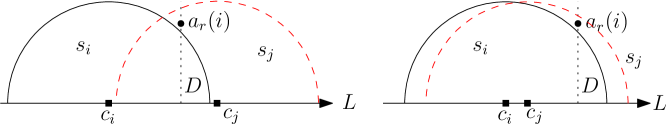
Figure 2: Illustrating the proof of Lemma 1. The red dashed half-circle is $s_{j}$ and the black solid half-circle is $s_{i}$. The two squares on $L$ are the centers of the two disks. Left: $c_{j}$ is to the right of point $a_{r}(i)$. Right: $c_{j}$ is to the left of point $a_{r}(i)$. In both cases, disk $s_{j}$ contains the region $D$.

Let $D$ be the region of $s_{i}$ to the right of the vertical line through $p_{k}$. By definition, $P_{r}(s_{i})=D\cap P$. Since $s_{i}$ and $s_{j}$ have the same radius and $s_{j}$ covers $p_{k}$ while $s_{i}$ does not, one can verify that $D$ must be contained in the disk $s_{j}$, regardless of whether $c_{j}$ is to the left or right of $p_{k}$ (e.g., see Fig. 2). Therefore, $s_{j}$ covers all points of $P_{r}(s_{i})$. ∎

The following lemma will help us to reduce the problem to the 1D problem.

Lemma 2

Suppose $S_{opt}$ is an optimal solution subset and $s_{i}$ is a disk in $S_{opt}$. Then, the following hold.

1. $s_{i}$ must be a useful disk.

2. $P_{m}(s_{i})$ has at least one point not covered by any disk of $S_{opt}\setminus\{s_{i}\}$.

3. All points of $P_{l}(s_{i})\cup P_{r}(s_{i})$ are covered by the disks of $S_{opt}\setminus\{s_{i}\}$.

Proof

First of all, since $s_{i}$ is in $S_{opt}$ and $w_{i}>0$, $s_{i}$ must cover a point $p^{*}\in P$ that is not covered by any other disk of $S_{opt}$. Depending on whether $a_{l}(i)=0$ and whether $a_{r}(i)=n+1$, there are several cases.

• If $a_{l}(i)=0$ and $a_{r}(i)=n+1$, then all points of $P$ are covered by $s_{i}$. Therefore, $S_{opt}$ has only one disk, which is $s_{i}$. Further, $a_{l}(i)=0$ and $a_{r}(i)=n+1$ imply that $P_{l}(s_{i})=P_{r}(s_{i})=\emptyset$. Hence, the lemma follows.

• If $a_{l}(i)\neq 0$ and $a_{r}(i)=n+1$, then some disk $s_{j}$ of $S_{opt}\setminus\{s_{i}\}$ must cover the point $a_{l}(i)$. Then, by Lemma 1, $s_{j}$ must cover all points of $P_{l}(s_{i})$. Hence, $p^{*}\not\in P_{l}(s_{i})$. Since $a_{r}(i)=n+1$, we have $P_{r}(s_{i})=\emptyset$. Thus, $p^{*}$ is in $P_{m}(s_{i})$. Therefore, the lemma follows.

• If $a_{l}(i)=0$ and $a_{r}(i)\neq n+1$, then the proof is analogous to the above second case and we omit it.

• If $a_{l}(i)\neq 0$ and $a_{r}(i)\neq n+1$, then by a similar proof as the above second case, we know that all points of $P_{l}(s_{i})$ are covered by a disk of $S_{opt}\setminus\{s_{i}\}$. Similarly, since $a_{r}(i)\neq n+1$, we can show that all points of $P_{r}(s_{i})$ are covered by a disk of $S_{opt}\setminus\{s_{i}\}$. This implies that $p^{*}$ is in $P_{m}(s_{i})$. Therefore, the lemma follows. ∎

By Lemma 2, to find an optimal solution, it is sufficient to consider only useful disks, and further, for each useful disk $s_{i}$, it is sufficient to assume that it only covers the points of $P_{m}(s_{i})=P[a_{l}(i)+1,a_{r}(i)-1]$. This observation leads to the following approach to reduce our problem to an instance of the 1D problem.

We assume that the indices $a_{l}(i)$ and $a_{r}(i)$ for all $i\in[1,m]$ are known. For each point $p_{i}$, we project it vertically on $L$, and let $P^{\prime}$ be the set of all projected points. For each useful disk $s_{i}$, we create a segment on $L$ whose left endpoint has $x$-coordinate equal to $x(p_{k+1})$ with $k=a_{l}(i)$ and whose right endpoint has $x$-coordinate equal to $x(p_{k^{\prime}-1})$ with $k^{\prime}=a_{r}(i)$, and the weight of the segment is equal to $w_{i}$. Let $S^{\prime}$ be the set of all segments thus defined. According to the above discussion, an optimal solution to the 1D problem on $P^{\prime}$ and $S^{\prime}$ corresponds to an optimal solution to our original problem on $P$ and $S$. By Theorem 3.1, the 1D problem can be solved in $O((n+m)\log(n+m))$ time because $|P^{\prime}|=n$ and $|S^{\prime}|\leq m$.

It remains to compute the indices $a_{l}(i)$ and $a_{r}(i)$ for all $i\in[1,m]$, which is done in the following lemma.

Lemma 3

Computing $a_{l}(j)$ and $a_{r}(j)$ for all $j\in[1,m]$ can be done in $O((n+m)\log(n+m))$ time.

Proof

We only describe how to compute $a_{r}(j)$ for all $j\in[1,m]$, and the algorithm for $a_{l}(j)$ is similar.

We sweep the plane with a vertical line $l$ from left to right, and an event happens if $l$ encounters a point of $P$ or a disk center. For this, we first sort all points of $P$ and all disk centers, in $O((n+m)\log(n+m))$ time. During the sweeping, we maintain a list $Q$ of disks $s_{i}$ whose centers have been swept and whose indices $a_{r}(i)$ have not been computed yet. $Q$ is just a first-in-first-out queue storing the disks ordered by their centers from left to right. Initially, $Q=\emptyset$.

During the sweeping, if $l$ encounters the center of a disk $s_{j}$, we add $s_{j}$ to the rear of $Q$. If $l$ encounters a point $p_{i}$, then we process it as follows. Starting from the front disk $s_{j}$ of $Q$, we check whether $s_{j}$ covers $p_{i}$. If yes, then one can verify that every disk in $Q$ covers $p_{i}$, and thus in this case we finish processing $p_{i}$. Otherwise, we remove $s_{j}$ from $Q$ and set $a_{r}(j)=i$, after which we proceed on the next disk in $Q$ (if $Q$ becomes $\emptyset$, then we finish processing $p_{i}$). If $Q$ is not empty after $p_{n}$ is processed, then we set $a_{r}(j)=n+1$ for all $s_{j}\in Q$.

The running time of the sweeping algorithm after sorting is $O(n+m)$. The lemma thus follows. ∎

With the preceding lemma, we have the following theorem.

Theorem 4.1

The line-constrained disk coverage problem for unit disks is solvable in $O((n+m)\log(n+m))$ time.

5 The $L_{1}$ case

In this case, each disk of $S$ is a diamond, whose boundary is comprised of four edges of slopes $1$ and $-1$, but the diamonds of $S$ may have different radii. We show that the problem can be solved in $O((n+m)\log(n+m))$ time by similar techniques to the unit-disk case in Section 4.

For each diamond $s_{i}\in S$, we still define the two indices $a_{l}(i)$ and $a_{r}(i)$ as well as the three subsets $P_{l}(s_{i})$, $P_{r}(s_{i})$, and $P_{m}(s_{i})$ in exactly the same way as in Section 4. We still call $s_{i}$ a useful disk if $a_{l}(i)+1<a_{r}(i)$.

Although the disks may have different radii, the geometric properties of the $L_{1}$ metric guarantee that Lemma 1 still applies. The proof is literally the same as before (indeed, one can verify that the region $D$ must be contained in the diamond $s_{j}$; e.g., see Fig. 3 as a counterpart of Fig. 2), so we omit it. As Lemma 2 mainly relies on Lemma 1, it also applies here. Consequently, once the indices $a_{r}(j)$ and $a_{l}(j)$ for all $j\in[1,m]$ are known, we can use the same algorithm as before to find an optimal solution in $O((n+m)\log(n+m))$ time. The algorithm for computing the indices $a_{r}(j)$ and $a_{l}(j)$, however, is not the same as before in Lemma 3. We provide a new algorithm in the following lemma.

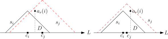
Figure 3: Illustrating the proof of Lemma 1 for the $L_{1}$ case, as a counterpart of Fig. 2. Now both $s_{i}$ and $s_{j}$ are diamonds (only the upper halves are shown). Left: $c_{j}$ is to the right of point $a_{r}(i)$. Right: $c_{j}$ is to the left of point $a_{r}(i)$. In both cases, $s_{j}$ contains the region $D$.

Lemma 4

Computing $a_{l}(j)$ and $a_{r}(j)$ for all $j\in[1,m]$ can be done in $O((n+m)\log(n+m))$ time.

Proof

We only describe how to compute $a_{r}(j)$ for all $i\in[1,m]$, and the algorithm for $a_{l}(i)$ is similar.

We sweep the plane with a vertical line $l$ from left to right, and an event happens if $l$ encounters a point of $P$ or the center of a diamond $s_{j}$. For this, we first sort all points of $P$ and the centers of all diamonds in $O((n+m)\log(n+m))$ time. During the sweeping, we maintain a list $Q$ of diamonds $s_{i}$ whose centers have been swept and whose indices $a_{r}(i)$ have not been computed yet. We store the diamonds of $Q$ by a balanced binary search tree with the $x$-coordinates of the rightmost points of the diamonds as the keys. Initially, $Q=\emptyset$.

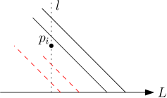
Figure 4: Illustrating an event when $l$ encounters a point $p_{i}\in P$. Four diamonds (only their upper right edges are shown) are in $Q$. To process the event, the two red dashed diamonds will be removed from $Q$, and their indices $a_{r}(j)$ will be set to $i$.

During to the sweeping, if $l$ encounters the center of a diamond $s_{j}$, then we insert $s_{j}$ into $Q$. If $l$ encounters a point $p_{i}$, then we process it as follows. Find the diamond $s_{j}$ in $Q$ with the smallest key (i.e., the diamond of $Q$ whose rightmost point is the leftmost). If $s_{j}$ covers $p_{i}$, then one can verify that every diamond in $Q$ covers $p_{i}$, and thus in this case we finish processing $p_{i}$. Otherwise (e.g., see Fig. 4), we delete $s_{j}$ from $Q$ and set $a_{r}(j)=i$, after which we proceed on the next diamond in $Q$ with the smallest key (if $Q$ becomes $\emptyset$, then we finish processing $p_{i}$). If $Q$ is not empty after $p_{n}$ is processed, then we set $a_{r}(j)=n+1$ for all $s_{j}\in Q$.

The running time of the sweeping algorithm after sorting is $O(n+m)$. The lemma thus follows. ∎

Theorem 5.1

The line-constrained disk coverage problem in the $L_{1}$ metric is solvable in $O((n+m)\log(n+m))$ time.

6 The $L_{\infty}$ and $L_{2}$ cases

In this section, we give our algorithms for the $L_{\infty}$ and $L_{2}$ cases. The algorithms are similar in the high level. However, the nature of the $L_{2}$ metric makes the $L_{2}$ case more involved in the low level computations. In Section 6.1, we present a high-level algorithmic scheme that works for both metrics. Then, we complete the algorithms for $L_{\infty}$ and $L_{2}$ cases in Sections 6.2 and 6.3, respectively.

6.1 An algorithmic scheme for $L_{\infty}$ and $L_{2}$ metrics

In this subsection, unless otherwise stated, all statements are applicable to both metrics. Note that a disk in the $L_{\infty}$ metric is a square.

For a disk $s_{k}\in S$, we say that a subsequence $P[i,j]$ of $P$ with $1\leq i\leq j\leq n$ is a maximal subsequence covered by $s_{k}$ if all points of $P[i,j]$ are covered by $s_{k}$ but neither $p_{i-1}$ nor $p_{j+1}$ is covered by $s_{k}$ (it is well defined due to $p_{0}$ and $p_{n+1}$). Let $F(s_{k})$ be the set of all maximal subsequences covered by $s_{k}$. Note that the subsequences of $F(s_{k})$ are pairwise disjoint.

Lemma 5

Suppose $S_{opt}$ is an optimal solution subset and $s_{k}$ is a disk of $S_{opt}$. Then, there is a subsequence $P[i,j]$ in $F(s_{k})$ such that the following hold.

1. $P[i,j]$ has a point that is not covered by any disk in $S_{opt}\setminus\{s_{k}\}$.

2. For any point $p\in P$ that is covered by $s_{k}$ but is not in $P[i,j]$, $p$ is covered by a disk in $S_{opt}\setminus\{s_{k}\}$.

Proof

First of all, $s_{k}$ must cover a point $p^{*}$ that is not covered by any disk in $S_{opt}\setminus\{s_{k}\}$. Since the subsequences of $F(s_{k})$ are pairwise disjoint, $p^{*}$ is in a unique subsequence $P[i,j]$ of $F(s_{k})$. In the following, we show that $P[i,j]$ has the property as stated in the lemma.

Consider any point $p_{h}\in P$ that is covered by $s_{k}$ but is not in $P[i,j]$. By the definition of maximal sequences, either $h\leq i-1$ or $h\geq j+1$. We only discuss the case $h\leq i-1$ since the other case is similar. In the following, we show that $p_{h}$ must be covered by a disk in $S_{opt}\setminus\{s_{k}\}$, which will prove the lemma.

Figure 5: Illustrating the proof of Lemma 5. The red dashed half-circle shows disk $s_{t}$, which covers $p_{i-1}$, and $x(c_{t})\leq x(c_{k}))$. The disk $s_{t}$ must also cover the point $p_{h}$.

By the definition of maximal sequences, neither $p_{i-1}$ nor $p_{j+1}$ is covered by $s_{k}$. Since $S_{opt}$ is an optimal solution, $S_{opt}\setminus\{s_{k}\}$ must have a disk $s_{t}$ that covers $p_{i-1}$. According to the above discussion, $s_{t}$ does not cover $p^{*}$. Since $p^{*}$ is to the right of $p_{i-1}$, the center $c_{t}$ of $s_{t}$ cannot be to the right of the center $c_{k}$ of $s_{k}$, since otherwise $s_{t}$ would cover $p^{*}$ as well because $s_{k}$ covers $p^{*}$. Let $D$ be the region of $s_{k}$ to the left of the vertical line through $p_{i-1}$. It is easy to see that $p_{h}$ is in $D$ (e.g., see Fig. 5). Since $x(c_{t})\leq x(c_{k})$ and $p_{i-1}$ is in $s_{t}$ but not in $s_{k}$, one can verify that $D$ is contained in $s_{t}$. Thus, $p_{h}$ must be covered by $s_{t}$. ∎

In light of Lemma 5, we reduce the problem to an instance of the 1D problem with a point set $P^{\prime}$ and a line segment set $S^{\prime}$, as follows.

For each point of $P$, we vertically project it on $L$, and the set $P^{\prime}$ is comprised of all such projected points. Thus $P^{\prime}$ has exactly $n$ points. For any $1\leq i\leq j\leq n$, we use $P^{\prime}[i,j]$ to denote the projections of the points of $P[i,j]$. For each point $p_{i}\in P$, we use $p_{i}^{\prime}$ to denote its projection point in $P^{\prime}$.

The set $S^{\prime}$ is defined as follows. For each disk $s_{k}\in S$ and each subsequence $P[i,j]\in F(s_{k})$, we create a segment for $S^{\prime}$, denoted by $s[i,j]$, with left endpoint at $p_{i}^{\prime}$ and right endpoint at $p^{\prime}_{j}$. Thus, $s[i,j]$ covers exactly the points of $P^{\prime}[i,j]$. We set the weight of $s[i,j]$ to $w_{k}$. Note that if $s[i,j]$ is already in $S^{\prime}$, which is defined by another disk $s_{h}$, then we only need to update its weight to $w_{k}$ in case $w_{k}<w_{h}$ (so each segment appears only once in $S^{\prime}$). We say that $s[i,j]$ is defined by $s_{k}$ (resp., $s_{h}$) if its weight is equal to $w_{k}$ (resp., $w_{h}$).

According to Lemma 5, we intend to say that an optimal solution $OPT^{\prime}$ to the 1D problem on $P^{\prime}$ and $S^{\prime}$ corresponds to an optimal solution $OPT$ to the original problem on $P$ and $S$ in the following sense: if a segment $s[i,j]\in S^{\prime}$ is included in $OPT^{\prime}$, then we include the disk that defines $s[i,j]$ in $OPT$. However, since a disk of $S$ may define multiple segments of $S^{\prime}$, to guarantee the correctness of the above correspondence, we need to show that $OPT^{\prime}$ is a valid solution: no two segments in $OPT^{\prime}$ are defined by the same disk of $S$. For this, we have the following lemma.

Lemma 6

Any optimal solution on $P^{\prime}$ and $S^{\prime}$ is a valid solution.

Proof

Let $OPT^{\prime}$ be any optimal solution. Let $s[i,j]$ be a segment in $OPT^{\prime}$. So $s[i,j]$ is defined by a disk $s_{k}$ for the maximal subsequence $P[i,j]$. In the following we show that no other segments defined by $s_{k}$ are in $OPT^{\prime}$, which will prove the lemma.

Assume to the contrary that $OPT^{\prime}$ has another segment $s[i^{\prime},j^{\prime}]$ defined by $s_{k}$. Then, since the maximal subsequences covered by $s_{k}$ are pairwise disjoint, either $j^{\prime}<i$ or $j<i^{\prime}$ holds. In the following, we only discuss the case $j^{\prime}<i$ since the other case is similar.

By the definition of maximal subsequences, neither $p_{j^{\prime}+1}$ nor $p_{i-1}$ is covered by $s_{k}$. Note that $j^{\prime}+1=i-1$ is possible. Hence, $OPT^{\prime}$ must have a segment $s^{\prime}$ defined by another disk $s_{h}$ covering $p_{i-1}$ such that $s^{\prime}$ covers the projection point $p^{\prime}_{i-1}$ of $p_{i-1}$. Since $s[i,j]$ is in $OPT^{\prime}$, $P^{\prime}[i,j]$ has at least one point $p^{*}$ that is not covered by any segment in $OPT^{\prime}$ other than $s[i,j]$. Thus, $p^{*}$ is not covered by $s^{\prime}$.

We claim that the center $c_{h}$ of $s_{h}$ is strictly to the left of the center of $c_{k}$ of $s_{k}$. Indeed, assume to the contrary that $x(c_{h})\geq x(c_{k})$. Then, let $D$ be the region of $s_{k}$ to the right of the vertical line through $p_{i-1}$. Notice that all points of $P[i,j]$ are in $D$. Also, since $s_{h}$ covers $p_{i-1}$ while $s_{k}$ does not and $x(c_{h})\geq x(c_{k})$, $D$ is contained in $s_{h}$. This means that all points of $P[i,j]$ are covered by $s_{h}$, and thus all points of $P[i-1,j]$ are covered by $s_{h}$ since $s_{h}$ covers $p_{i-1}$. Hence, the segment $s^{\prime}$ covers all points of $P^{\prime}[i-1,j]$, and thus, $s^{\prime}$ covers the points $p^{*}$, which contradicts with the fact that $s^{\prime}$ does not cover $p^{*}$. This proves the claim that $x(c_{h})<x(c_{k})$.

Depending on whether $s_{h}$ covers all points of $P[j^{\prime}+1,i-1]$, there are two cases.

• If $s_{h}$ covers all points of $P[j^{\prime}+1,i-1]$, then since $x(c_{h})<x(c_{k})$ and $s_{k}$ does not cover $p_{j^{\prime}+1}$ (but covers all points of $P[i^{\prime},j^{\prime}]$), by the similar analysis as above, we can show that $s_{h}$ also covers all points of $P[i^{\prime},j^{\prime}]$ and thus all points of $P[i^{\prime},i-1]$. This implies that the segment $s^{\prime}$ covers all projection points of $P^{\prime}[i^{\prime},i-1]$. Therefore, if we remove $s[i^{\prime},j^{\prime}]$ from $OPT^{\prime}$, the remaining segments of $OPT^{\prime}$ still cover all points of $P^{\prime}$, which contradicts with that $OPT^{\prime}$ is an optimal solution.

• If $s_{h}$ does not cover all points of $P[j^{\prime}+1,i-1]$, then let $h_{1}$ be the largest index in $[j^{\prime}+1,i-2]$ such that $p_{h_{1}}$ is not covered by $s_{h}$. Then, $p_{h_{1}}^{\prime}$ is not covered by the segment $s^{\prime}$. Hence, $OPT^{\prime}$ must have a segment defined by another disk $s_{j_{1}}$ covering $p_{h_{1}}$ such that the segment covers $p_{h_{1}}^{\prime}$. By the same analysis as above, we can show that $x(c_{j_{1}})<x(c_{h})$, and thus $x(c_{j_{1}})<x(c_{k})$.

  If $s_{j_{1}}$ covers all points of $P[j^{\prime}+1,h_{1}-1]$, then we can use the same analysis as the above case to show that $s[i^{\prime},j^{\prime}]$ is a redundant segment of $OPT^{\prime}$, which incurs contradiction. Otherwise, we let $h_{2}$ be the largest index in $[j^{\prime}+1,h_{1}-1]$ such that $p_{h_{2}}$ is not covered by $s_{j_{1}}$. Then, we can follow the same analysis above to either obtain contradiction or consider the next index in $[j^{\prime}+1,h_{2}-1]$. Note that this procedure is finite as the number of indices of $[j^{\prime}+1,h_{1}-1]$ is finite. Therefore, eventually we will obtain contradiction.

The lemma thus follows. ∎

With the above lemma, combining with our algorithm for the 1D problem, we have the following result.

Lemma 7

If the set $S^{\prime}$ is computed, then an optimal solution can be found in $O((n+|S^{\prime}|)\log(n+|S^{\prime}|))$ time.

It remains to determine the size of $S^{\prime}$ and compute $S^{\prime}$. An obvious answer is that $|S^{\prime}|$ is bounded by $m\cdot\lceil n/2\rceil$ because each disk can have at most $\lceil n/2\rceil$ maximal sequences of $P$, and a trivial algorithm can compute $S^{\prime}$ in $O(nm\log(m+n))$ time by scanning the sorted list $P$ for each disk. Therefore, by Lemma 7, we can solve the problem in both $L_{\infty}$ and $L_{2}$ metrics in $O(nm\log(m+n))$ time.

With more geometric observations, the following two subsections will prove the two following lemmas, respectively.

Lemma 8

In the $L_{\infty}$ metric, $|S^{\prime}|\leq 2(n+m)$ and $S^{\prime}$ can be computed in $O((n+m)\log(n+m))$ time.

Lemma 9

In the $L_{2}$ metric, $|S^{\prime}|\leq 2(n+m)+\kappa$ and $S^{\prime}$ can be computed in $O((n+m)\log(n+m)+\kappa\log m)$ time.

With Lemma 7, we have the following results.

Theorem 6.1

The line-constrained disk coverage problem in the $L_{\infty}$ metric is solvable in $O((n+m)\log(n+m))$ time.

Theorem 6.2

The line-constrained disk coverage problem in the $L_{2}$ metric is solvable in $O(nm\log(m+n))$ time or in $O((n+m)\log(n+m)+\kappa\log m)$ time, where $\kappa$ is the number of pairs of disks of $S$ that intersect each other.

Bounding couples.

Before moving on, we introduce a new concept bounding couples, which will be used to prove Lemmas 8 and 9 in Sections 6.2 and 6.3.

Consider a disk $s_{k}\in S$. Let $p_{l}(s_{k})$ denote the rightmost point of $P\cup\{p_{0},p_{n+1}\}$ strictly to the left of $l_{k}$; similarly, let $p_{r}(s_{k})$ denote the leftmost point of $P\cup\{p_{0},p_{n+1}\}$ strictly to the right of $r_{k}$. Let $P(s_{k})$ denote the subset of points of $P$ between $p_{l}(s_{k})$ and $p_{r}(s_{k})$ inclusively that are outside $s_{k}$. We sort the points of $P(s_{k})$ by their $x$-coordinates, and we call each adjacent pair of points (or their indices) in the sorted list a bounding couple (e.g., see Fig. 6). Let $C(s_{k})$ denote the set of all bounding couples of $s_{k}$, and for each bounding couple of $C(s_{k})$, we assign $w_{k}$ to it as the weight. Let $\mathcal{C}=\bigcup_{1\leq k\leq m}C(s_{k})$, and if the same bounding couple is defined by multiple disks, then we only keep the copy in $\mathcal{C}$ with the minimum weight. Also, we consider a bounding couple $(i,j)$ as an ordered pair such that $i<j$, and $i$ is considered as the left end of the couple while $j$ is the right end.

Figure 6: Illustrating the definition of bounding couples: the numbers are the indices of the points of $P$. In this example, $p_{l}(s_{k})$ is point $2$ and $p_{r}(s_{k})$ is point $11$, and the bounding couples are: $(2,3)$, $(3,5)$, $(5,7)$, $(7,10)$, $(10,11)$.

The reason why we define bounding couples is that if $P[i,j]$ is a maximal subsequence of $P$ covered by $s_{k}$ then $(i-1,j+1)$ is a bounding couple. On the other hand, if $(i,j)$ is a bounding couple of $C(s_{k})$, then $P[i+1,j-1]$ is a maximal subsequence of $P$ covered by $s_{k}$ unless $j=i+1$. Hence, each bounding couple $(i,j)$ of $\mathcal{C}$ with $j\neq i+1$ corresponds to a segment in the set $S^{\prime}$, and $|S^{\prime}|\leq|\mathcal{C}|$. Observe that $\mathcal{C}$ has at most $n-1$ couples $(i,j)$ with $j=i+1$, and given $\mathcal{C}$, we can obtain $S^{\prime}$ in additional $O(|\mathcal{C}|)$ time.

According to our above discussion, to prove Lemmas 8 and 9, it suffices to prove the following two lemmas.

Lemma 10

In the $L_{\infty}$ metric, $|\mathcal{C}|\leq 2(n+m)$ and $\mathcal{C}$ can be computed in $O((n+m)\log(n+m))$ time.

Lemma 11

In the $L_{2}$ metric, $|\mathcal{C}|\leq 2(n+m)+\kappa$ and $\mathcal{C}$ can be computed in $O((n+m)\log(n+m)+\kappa\log m)$ time.

Consider a bounding couple $(i,j)$ of $\mathcal{C}$, defined by a disk $s_{k}$. We call it a left bounding couple if $p_{i}=p_{l}(s_{k})$, a right bounding couple if $p_{j}=p_{r}(s_{k})$, and a middle bounding couple otherwise (e.g., in Fig. 6, $(2,3)$ is the left bounding couple, $(10,11)$ is the right bounding couple, and the rest are middle bounding couples). It is easy to see that a disk can define at most one left bounding couple and at most one right bounding couple. Therefore, the number of left and right bounding couples in $\mathcal{C}$ is at most $2m$. It remains to bound the number of middle bounding couples of $\mathcal{C}$.

In the following, we will prove Lemmas 10 and 11 in Sections 6.2 and 6.3, respectively.

6.2 The $L_{\infty}$ metric

In this section, our goal is to prove Lemma 10.

In the $L_{\infty}$ metric, every disk is a square that has four axis-parallel edges. We use $l_{k}$ and $r_{k}$ to particularly refer to the left and right endpoints of the upper edge of $s_{k}$, respectively.

For a point $p_{i}$ and a square $s_{k}$, we say that $p_{i}$ is vertically above (resp., below) the upper edge of $s_{k}$ if $p_{i}$ is above (resp., below) the upper edge of $s_{k}$ and $x(l_{k})\leq x(p_{i})\leq x(r_{k})$. Due to our general position assumption, $p_{i}$ is not on the boundary of $s_{k}$, and thus $p_{i}$ above/below the upper edge of $s_{k}$ implies that $p_{i}$ is strictly above/below the edge. Also, since no point of $P$ is below $L$, a point $p_{i}\in P$ is in $s_{k}$ if and only if $p_{i}$ is vertically below the upper edge of $s_{k}$. If $p_{i}$ is vertically above the upper edge of $s_{k}$, we also say that $p_{i}$ is vertically above $s_{k}$ or $s_{k}$ is vertically below $p_{i}$.

The following lemma proves an upper bound for $|\mathcal{C}|$.

Lemma 12

$|\mathcal{C}|\leq 2(n+m)$.

Proof

Recall that the total number of left and right bounding couples of $\mathcal{C}$ is at most $2m$. In the following, we show that the number of middle bounding couples of $\mathcal{C}$ is at most $2n$.

We first prove an observation: For each point $p_{j}$ of $P$, among all points of $P$ to the northwest of $p_{j}$, there is at most one point that can form a middle bounding couple with $p_{j}$; similarly, among all points of $P$ to the northeast of $p_{j}$, there is at most one point that can form a middle bounding couple with $p_{j}$.

We only prove the northwest case since the other case is analogous. Suppose there is a point $p_{i}\in P$ to the northwest of $p_{j}$ and $(p_{i},p_{j})$ is a middle bounding couple. Assume to the contrary that there is another point $p_{h}\in P$ to the northwest of $p_{j}$ and $(p_{h},p_{j})$ is a middle bounding couple defined by a disk $s_{k}$. Without loss of generality, we assume $h<i$.

Since $(p_{h},p_{j})$ is a middle bounding couple, both $p_{h}$ and $p_{j}$ are vertically above $s_{k}$. Since $p_{i}$ is to the northwest of $p_{j}$ and $h<i<j$, $p_{i}$ is also vertically above $s_{k}$. But then $p_{i}$ would prevent $(h,j)$ from being a middle bounding couple defined by $s_{k}$, incurring contradiction. This proves the observation.

We proceed to show that the number of middle bounding couples is at most $2n$. Indeed, for any middle bounding couple $(i,j)$ of $\mathcal{C}$, we charge it to the lower point of $p_{i}$ and $p_{j}$. In light of the observation, each point of $P$ will be charged at most twice. As such, the total number of middle bounding couples is at most $2n$. The lemma thus follows. ∎

We proceed to compute the set $\mathcal{C}$. The following lemma gives an algorithm to compute all left and right bounding couples of $\mathcal{C}$.

Lemma 13

All left and right bounding couples of $\mathcal{C}$ can be computed in $O((n+m)\log(n+m))$ time.

Proof

We only describe how to compute all left bounding couples, and the algorithm for computing the right bounding couples is similar.

First of all, we compute the points $p_{l}(s_{k})$ and $p_{r}(s_{k})$ for all $k=1,2,\ldots,m$. Each such point can be computed in $O(\log n)$ time by binary search on the sorted sequence of $P$. Hence, computing all such points takes $O(m\log n)$ time. To compute all left bounding couples, it is sufficient to compute the points $p(s_{k})$ for all disks $s_{k}\in S$, where $p(s_{k})$ is the leftmost point of $P$ outside $s_{k}$ and between $l_{k}$ and $r_{k}$ if it exists and $p(s_{k})$ is $p_{r}(s_{k})$ otherwise, because $(p_{l}(s_{k}),p(s_{k}))$ is the left bounding couple defined by $s_{k}$. To this end, we propose the following algorithm.

We sweep a vertical line $l$ from left to right, and an event happens if $l$ encounters a point of $P\cup\{l_{k},r_{k}|\ 1\leq k\leq m\}$. For this, we first sort all points of $P\cup\{l_{k},r_{k}|\ 1\leq k\leq m\}$. During the sweeping, we use a balanced binary search tree $T$ to maintain those disks $s_{k}$ intersecting $l$ whose points $p(s_{k})$ have not been computed yet. The disks in $T$ are ordered by the $y$-coordinates of their upper edges.

During the sweeping, if $l$ encounters the left endpoint $l_{k}$ of a disk $s_{k}$, we insert $s_{k}$ into $T$. If $l$ encounters the right endpoint $r_{k}$ of $s_{k}$, we remove $s_{k}$ from $T$ and set $p(s_{k})=p_{r}(s_{k})$. If $l$ encounters a point $p_{i}$ of $P$, then for each disk $s_{k}$ of $T$ whose upper edge is below $p_{i}$, we set $p(s_{k})=p_{i}$ and remove $s_{k}$ from $T$.

It is not difficult to see that the algorithm correctly computes all points $p(s_{k})$ for all $s_{k}\in S$ in $O((n+m)\log(m+n))$ time. The lemma thus follows. ∎

In the following, we focus on computing all middle bounding couples of $\mathcal{C}$.

6.2.1 Computing the middle bounding couples

We sweep a vertical line $l$ from left to right, and an event happens if $l$ encounters a point in $P\cup\{l_{k},r_{k}|\ 1\leq k\leq m\}$. Let $H$ be the set of disks that intersect $l$. During the sweeping, we maintain the following information and invariants (e.g., see Fig. 7).

Figure 7: Illustrating the information maintained by our sweeping algorithm. $P(l)=\{p_{i_{1}},p_{i_{2}},p_{i_{3}},p_{i_{4}}\}$. Each horizontal segment represents the upper edge of a disk. $H(i_{1})$ consists of two blue disks and $H(i_{4})$ consists of two red disks. $H_{0}$ consists of three black disks.

1. A sequence $P(l)=\{p_{i_{1}},p_{i_{2}},\ldots,p_{i_{t}}\}$ of $t$ points of $P$, which are to the left of $l$ and ordered from northwest to southeast. $P(l)$ is stored in a balanced binary search tree $T(P(l))$.

2. A collection $\mathcal{H}$ of $t+1$ subsets of $H$: $H(i_{j})$ for $j=0,1,\ldots,t$, which form a partition of $H$, defined as follows.

   $H(i_{t})$ is the subset of disks of $H$ that are vertically below $p_{i_{t}}$. For each $j=t-1,t-2,\ldots,1$, $H(i_{j})$ is the subset of disks of $H\setminus\bigcup^{t}_{k=j+1}H(i_{k})$ that are vertically below $p_{i_{j}}$. $H(i_{0})=H\setminus\bigcup^{t}_{j=1}H(i_{j})$. While $H(i_{0})$ may be empty, none of $H(i_{j})$ for $1\leq j\leq t$ is empty.

   Each set $H(i_{j})$ is maintained by a balanced binary search tree $T(H(i_{j}))$ ordered by the $y$-coordinates of the upper edges of the disks. We have all disks stored in leaves of $T(H(i_{j}))$, and each internal node $v$ of the tree also stores a weight equal to the minimum weight of all disks in the leaves of the subtree rooted at $v$.

3. For each point $p_{i_{j}}\in P(l)$, among all points of $P$ strictly between $p_{i_{j}}$ and $l$, no point is vertically above any disk of $H(i_{j})$.

4. Among all points of $P$ strictly to the left of $l$, no point is vertically above any disk of $H(i_{0})$.

In summary, our algorithm maintains the following trees: $T(P(l))$, $T(H(i_{j}))$ for all $j\in[0,t]$.

Initially when $l$ is to the left of all disks and points of $P$, we have $H=\emptyset$ and $P(l)=\emptyset$. We next describe how to process events.

If $l$ encounters the left endpoint $l_{k}$ of a disk $s_{k}$, we insert $s_{k}$ to $H(i_{0})$. The time for processing this event is $O(\log m)$ since $|H(i_{0})|\leq m$.

If $l$ encounters the right endpoint $r_{k}$ of a disk $s_{k}$, we need to determine which set $H(i_{j})$ of $\mathcal{H}$ contains $s_{k}$. For this, we associate each right endpoint with its disk in the preprocessing so that it can keep track of which set of $\mathcal{H}$ contains the disk. Using this mechanism, we can determine the set $H(i_{j})$ that contains $s_{k}$ in constant time. We then remove $s_{k}$ from $T(H(i_{j}))$. If $H(i_{j})$ becomes empty and $j\neq 0$, then we remove $p_{i_{j}}$ from $P(l)$. One can verify that all algorithm invariants still hold. The time for processing this event is $O(\log(m+n))$.

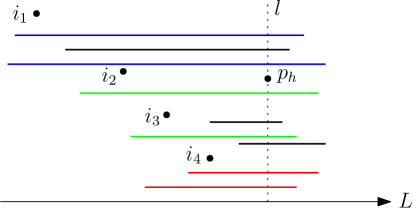
Figure 8: Illustrating the processing of an event at $p_{h}\in P$. In this example, $i_{2}$, $i_{3}$, and $i_{4}$ will be removed from $P(l)$ and $p_{h}$ will be inserted to $P(l)$, so after the event $P(l)=\{p_{i_{1}},p_{h}\}$. Also, $(i_{2},h)$, $(i_{3},h)$, $(i_{4},h)$ will be reported as middle bounding couples.

If $l$ encounters a point $p_{h}$ of $P$, which is a major event we need to handle, we process it as follows. We search $T(P(l))$ to find the first point $p_{i_{j}}$ of $P(l)$ below $p_{h}$ (e.g., $j=3$ in Fig. 8). We remove the points $p_{i_{k}}$ for all $k\in[j,t]$ from $P(l)$. We have the following lemma.

Lemma 14

For each point $p_{i_{k}}$ with $k\in[j,t]$, $(i_{k},h)$ is a middle bounding couple defined by and only by the disks of $H(i_{k})$ (i.e., $H(i_{k})$ consists of all disks of $S$ that define $(i_{k},h)$ as a middle bounding couple).

Proof

By the definition of $H(i_{k})$, $p_{i_{k}}$ is vertically above each disk of $H(i_{k})$. By the definition of $j$ and also because all disks of $H(i_{k})$ intersect $l$, $p_{h}$ is vertically above each disk of $H(i_{k})$. With the third algorithm invariant, $(i_{k},h)$ is a middle bounding couple defined by every disk of $H(i_{k})$.

On the other hand, suppose a disk $s$ defines $(i_{k},h)$ as a middle bounding couple. Then, both $p_{i_{k}}$ and $p_{h}$ must be vertically above $s$. This implies that $s$ intersects $l$, and thus $s$ is in $H$. By algorithm invariant (4), $s$ cannot be in $H(i_{0})$. Because $p_{i_{k}}$ is vertically above $s$, $s$ must be in $\bigcup_{b=k}^{t}H(i_{b})$. Further, since $(i_{k},h)$ is a middle bounding couple, among all points of $P$ strictly between $p_{i_{k}}$ and $p_{h}$, no point is vertically above $s$. This implies that $s$ cannot be in $H(i_{b})$ for any $b>k$. Therefore, $s$ must be in $H(i_{k})$. The lemma thus follows. ∎

In light of Lemma 14, for each $k\in[j,t]$, we report $(i_{k},h)$ as a middle bounding couple with weight equal to the minimum weight of all disks of $H(i_{k})$, which is stored at the root of $T(H(i_{k}))$.

Next, we process the point $p_{i_{j-1}}$, for which we have the following lemma. The proof technique is similar to that for Lemma 14, so we omit it.

Lemma 15

If $p_{h}$ is vertically below the lowest disk of $H(i_{j-1})$, then $(i_{j-1},h)$ is not a middle bounding couple; otherwise, $(i_{j-1},h)$ is a middle bounding couple defined by and only by disks of $H_{j-1}$ that are vertically below $p_{h}$.

By the above lemma, we first check whether $p_{h}$ is vertically below the lowest disk of $H(i_{j-1})$. If yes, we do nothing. Otherwise, we report $(i_{j-1},h)$ as a middle bounding couple with weight equal to the minimum weight of all disks of $H(i_{j-1})$ vertically below $p_{h}$, which can be computed in $O(\log m)$ time by using weights at the internal nodes of $T(H(i_{j-1}))$. We further have the following lemma.

Lemma 16

If all disks of $H(i_{j-1})$ are vertically below $p_{h}$, then there does not exist a middle bounding couple $({i_{j-1}},b)$ with $b>h$.

Proof

Assume to the contrary that $(i_{j-1},b)$ is such a middle bounding couple with $b>h$, say, defined by a disk $s$. Then, since $x(p_{i_{j-1}})<x(p_{h})=x(l)<x(p_{b})$, $s$ intersects $l$, and thus $s$ is in $H$. Also, since $s$ defines the couple, $p_{i_{j-1}}$ is vertically above $s$. Note that all disks of $H$ vertically below $p_{i_{j-1}}$ must be in $\bigcup_{k=j-1}^{t}H(i_{k})$, and thus $s$ is in $\bigcup_{k=j-1}^{t}H(i_{k})$. Recall that all disks of $\bigcup_{k=j}^{t}H(i_{k})$ are vertically below $p_{h}$. Since all disks of $H(i_{j-1})$ are vertically below $p_{h}$, all disks of $\bigcup_{k=j-1}^{t}H(i_{k})$ are vertically below $p_{h}$. Hence, $s$ is also vertically below $p_{h}$. Because all three points $p_{i_{j-1}}$, $p_{h}$, and $p_{b}$ are vertically above $s$, and $x(p_{i_{j-1}})<x(p_{h})<x(p_{b})$, $(i_{j-1},b)$ cannot be a bounding couple defined by $s$. The lemma thus follows. ∎

We check whether $p_{h}$ is above the highest disk of $H(i_{j-1})$ using the tree $T(H(i_{j-1}))$. If yes, then the above lemma tells that there will be no more middle bounding couples involving $i_{j-1}$ any more, and thus we remove $p_{i_{j-1}}$ from $P(l)$.

The following lemma implies that all middle bounding couples with $p_{h}$ as the right end have been computed.

Lemma 17

For any middle bounding couple $(b,h)$, $b$ must be in $\{i_{j-1},i_{j},\ldots,i_{t}\}$.

Proof

Assume to the contray that $(b,h)$ is a middle bounding couple with $b$ not in the set $\{i_{j-1},i_{j},\ldots,i_{t}\}$, say, defined by a disk $s$. Then, $s$ must intersect $l$, and thus is in $H$. Also, $s$ is vertically below both $p_{b}$ and $p_{h}$.

First of all, since $p_{b}$ is strictly to the left of $l$ and $p_{b}$ is vertically above $s$, by our algorithm invariant (4), $s$ cannot be in $H(i_{0})$. Thus, $s$ is in $H(i_{j})$ for some $j\in[1,t]$. Depending on whether $i_{j}<b$, there are two cases.

If $i_{j}>b$, then since $s\in H(i_{j})$, $p_{i_{j}}$ is vertically above $s$. Because $x(p_{b})<x(p_{i_{j}})<x(p_{h})$ and all these three points are vertically above $s$, $(b,h)$ cannot be a middle bounding couple defined by $s$, incurring contradiction.

If $i_{j}<b$, then since $s\in H(i_{j})$ and $p_{b}$ is vertically above $s$, we obtain contradiction with our algorithm invariant (3) as $p_{b}$ is strictly between $p_{i_{j}}$ and $l$. ∎

Next, we add $p_{h}$ to the end of the current sequence $P(l)$ (note that the points $p_{i_{k}}$ for all $k\in[j,t]$ and possibly $p_{i_{j-1}}$ have been removed from $P(l)$; e.g., see Fig. 8). Finally, we need to compute the tree $T(H(h))$ for the set $H(h)$, which is comprised of all disks of $H$ vertically below $p_{h}$ since $p_{h}$ is the lowest point of $P(l)$. We compute $T(H(h))$ as follows.

First, starting from an empty tree, for each $k=t,t-1,\dots,j$ in this order, we merge $T(H(h))$ with the tree $T(H(i_{k}))$. Notice that the upper edge of each disk in $T(H(i_{k}))$ is higher than the upper edges of all disks of $T(H(h))$. Therefore, each such merge operation can be done in $O(\log m)$ time. Second, for the tree $T(H(i_{j-1}))$, we perform a split operation to split the disks into those with upper edges above $p_{h}$ and those below $p_{h}$, and then merge those below $p_{h}$ with $T(H(h))$ while keeping those above $p_{h}$ in $T(H(i_{j-1}))$. The above split and merge operations can be done in $O(\log m)$ time. Third, we remove those disks below $p_{h}$ from $H(i_{0})$ and insert them to $T(H(h))$. This is done by repeatedly removing the lowest disk $s$ from $H(i_{0})$ and inserting it to $T(H(h))$ until the upper edge of $s$ is higher than $p_{h}$. This completes our construction of the tree $T(H(h))$.

The above describes our algorithm for processing the event at $p_{h}$. One can verify that all algorithm invariants still hold. The running time of this step is $O((1+k_{1}+k_{2})\log m)$ time, where $k_{1}$ is the number of points removed from $P(l)$ (the number of merge operations is at most $k_{1}$) and $k_{2}$ is the number of disks of $H(i_{0})$ got removed for constructing $T(H(h))$. As we sweep the line $l$ from left to right, once a point is removed from $P(l)$, it will not be inserted again, and thus the total sum of $k_{1}$ in the entire algorithm is at most $n$. Also, once a disk is removed from $H(i_{0})$, it will never be inserted again, and thus the total sum of $k_{2}$ in the entire algorithm is at most $m$. Hence, the overall time of the algorithm is $O((n+m)\log(n+m))$. This proves Lemma 10.

6.3 The $L_{2}$ metric

In this section, our goal is to prove Lemma 11.

Recall our general position assumption that no point of $P$ is on the boundary of a disk of $S$. Also recall that all points of $P$ are above $L$. In the $L_{2}$ metric, the two extreme points $l_{k}$ and $r_{k}$ of a disk $s_{k}$ are unique. For a point $p_{i}\in P$ and a disk $s_{k}\in S$, we say that $p_{i}$ is vertically above $s_{k}$ if $p_{i}$ is outside $s_{k}$ and $x(l_{k})\leq x(p_{i})\leq x(r_{k})$, and $p_{i}$ is vertically below $s_{k}$ if $p_{i}$ is inside $s_{k}$. We also say that $s_{k}$ is vertically below $p_{i}$ if $p_{i}$ is vertically above $s_{k}$.

The following lemma gives an upper bound for $|\mathcal{C}|$.

Lemma 18

$|\mathcal{C}|\leq 2(n+m)+\kappa$.

Proof

Recall that the left and right bounding couples of $\mathcal{C}$ is at most $2m$. Let $\mathcal{C}_{m}$ denote the set of all middle bounding couples of $\mathcal{C}$. In the following, we argue that $|\mathcal{C}_{m}|\leq 2n+\kappa$.

For convenience, we consider a middle bounding couple $(i,j)$ as a bounding interval $[i,j]$ defined on indices of $P$. We call the indices larger than $i$ and smaller than $j$ as the interior of the interval. Those indices smaller than $i$ and larger than $j$ are considered outside the interval.

We say that two bounding intervals $[a,b]$ and $[a^{\prime},b^{\prime}]$ conflict if either $a<a^{\prime}<b<b^{\prime}$ or $a^{\prime}<a<b^{\prime}<b$. Hence, those two intervals do not conflict if either they are interior-disjoint or one interval contains the other. Since two bounding intervals defined by the same disk are interior-disjoint, they never conflict.

We first prove an observation: For any two disks, there is at most one pair of conflicting bounding intervals defined by the two disks.

Assume to the contrary there are two pairs of conflicting bounding intervals defined by two disks $s$ and $s^{\prime}$. Let the first pair be $[a,b]$ and $[a^{\prime},b^{\prime}]$ and the second pair be $[c,d]$ and $[c^{\prime},d^{\prime}]$. Without loss of generality, we assume that $[a,b]$ and $[c,d]$ are defined by $s$, and $[a^{\prime},b^{\prime}]$ and $[c^{\prime},d^{\prime}]$ are defined by $s^{\prime}$. Note that $[a,b]$ and $[c,d]$ may be the same and $[a^{\prime},b^{\prime}]$ and $[c^{\prime},d^{\prime}]$ may also be the same. However, as they are different pairs, either $[a,b]$ and $[c,d]$ are distinct, or $[a^{\prime},b^{\prime}]$ and $[c^{\prime},d^{\prime}]$ are distinct. Without loss of generality, we assume that $[a,b]$ and $[c,d]$ are distinct and $b\leq c$. Depending on whether $[a^{\prime},b^{\prime}]$ and $[c^{\prime},d^{\prime}]$ are the same, there are two cases.

• If $[a^{\prime},b^{\prime}]$ and $[c^{\prime},d^{\prime}]$ are the same, then since $b\leq c$, we have $a<a^{\prime}<b\leq c<b^{\prime}<d$ (see Fig. 10). By the definition of bounding intervals, $p_{b}$ and $p_{c}$ are in the disk $s^{\prime}$ while $p_{a^{\prime}}$ and $p_{b^{\prime}}$ are vertically above $s^{\prime}$, and similarly, $p_{a^{\prime}}$ and $p_{b^{\prime}}$ are in the disk $s$ while $p_{a},p_{b},p_{c},p_{d}$ are vertically above $s$.

  

  Figure 9: Illustrating the conflicting intervals: Each arc represents an interval.

  

  Figure 10: Illustrating the disk $s^{\prime}$ and points $a^{\prime}$, $b^{\prime}$, $b$, $q_{a^{\prime}b}$, and $q_{bb^{\prime}}$.

  Since $p_{b}$ is contained in $s^{\prime}$ while $p_{a^{\prime}}$ and $p_{b^{\prime}}$ are vertically above $s^{\prime}$ (e.g., see Fig. 10), we claim that any disk centered at $L$ and containing both $p_{a^{\prime}}$ and $p_{b^{\prime}}$ must contain the point $p_{b}$. Indeed, let $q_{a^{\prime}b}$ be the point on $L$ that has the same distance with $p_{a^{\prime}}$ and $p_{b}$, and let $q_{bb^{\prime}}$ be the point on $L$ that has the same distance with $p_{b}$ and $p_{b^{\prime}}$ (e.g., see Fig. 10). Since $x(p_{a^{\prime}})<x(p_{b})$ and $p_{b}$ is in $s^{\prime}$ while $p_{a^{\prime}}$ is not, we can obtain that $x(q_{a^{\prime}b})<x(c^{\prime})$, where $c^{\prime}$ is the center of $s^{\prime}$. For the same reason, $x(q_{bb^{\prime}})>x(c^{\prime})$. Therefore, $q_{a^{\prime}b}$ is strictly to the left of $q_{bb^{\prime}}$. Now consider any disk $s^{\prime\prime}$ with center $c^{\prime\prime}$ at $L$ such that $s^{\prime\prime}$ contains both $p_{a^{\prime}}$ and $p_{b^{\prime}}$. If $x(c^{\prime\prime})\leq x(q_{a^{\prime}b})$, then $x(c^{\prime\prime})<x(q_{bb^{\prime}})$ and thus $c^{\prime\prime}$ is closer to $p_{b}$ than to $p_{b^{\prime}}$. Since $s^{\prime\prime}$ contains $p_{b^{\prime}}$, $s^{\prime\prime}$ also contains $p_{b}$. On the other hand, if $x(c^{\prime\prime})>x(q_{a^{\prime}b})$, then $c^{\prime\prime}$ is closer to $p_{b}$ than to $p_{a^{\prime}}$. Since $s^{\prime\prime}$ contains $p_{a^{\prime}}$, $s^{\prime\prime}$ also contains $p_{b}$. This proves the claim.

  Recall that the disk $s$ contains $p_{a^{\prime}}$ and $p_{b^{\prime}}$. By the above claim, $s$ contains $p_{b}$, but this contradicts with that $p_{b}$ is strictly above $s$.

• If $[a^{\prime},b^{\prime}]$ and $[c^{\prime},d^{\prime}]$ are not the same, then without loss of generality, we assume that $b^{\prime}\leq c^{\prime}$. Since $[a,b]$ conflicts with $[a^{\prime},b^{\prime}]$, either $a<a^{\prime}<b<b^{\prime}$ or $a^{\prime}<a<b^{\prime}<b$. Similarly, since $[c,d]$ conflicts with $[c^{\prime},d^{\prime}]$, either $c<c^{\prime}<d<d^{\prime}$ or $c^{\prime}<c<d^{\prime}<d$. In the following, we assume that $a<a^{\prime}<b<b^{\prime}$ and $c<c^{\prime}<d<d^{\prime}$ (e.g., see Fig. 11), and the other cases can be proved in a similar way.

  

  Figure 11: Illustrating the conflicting intervals: Each arc represents an interval. The intervals of solid (resp., dotted) arcs are defined by $s$ (resp., $s^{\prime}$).

  Since $c<c^{\prime}<d$ and $b^{\prime}\leq c^{\prime}$, we obtain that $a^{\prime}<b<c^{\prime}$. Since $[a^{\prime},b^{\prime}]$ and $[c^{\prime},d^{\prime}]$ are bounding intervals defined by the disk $s^{\prime}$ while $b$ is in the interior of $[a^{\prime},b^{\prime}]$, $s^{\prime}$ contains $p_{b}$ but is vertically below $p_{a^{\prime}}$ and $p_{c^{\prime}}$. Then, by the claim proved in the first case, any disk centered at $L$ and containing both $p_{a^{\prime}}$ and $p_{c^{\prime}}$ must contain $p_{b}$ as well.

  On the other hand, since $[a,b]$ and $[c,d]$ are bounding intervals defined by $s$ while $a^{\prime}$ is in the interior of $[a,b]$ and $c^{\prime}$ is in the interior of $[c,d]$, $s$ contains both $p_{a^{\prime}}$ and $p_{c^{\prime}}$ but is vertically below $p_{b}$. However, since $s$ contains both $p_{a^{\prime}}$ and $p_{c^{\prime}}$ and $s$ is centered at $L$, according to the above claim, $s$ contains $p_{b}$. Therefore, we obtain contradiction.

This proves the observation.

We then prove another observation: If a bounding interval defined by a disk conflicts with a bounding interval defined by another disk, then the two disks must intersect.

Indeed, suppose two bounding intervals $[a,b]$ and $[a^{\prime},b^{\prime}]$ conflict. Let $s$ be the disk defining $[a,b]$ and $s^{\prime}$ be the disk defining $[a^{\prime},b^{\prime}]$. Without loss of generality, we assume that $a<a^{\prime}<b<b^{\prime}$. By the definition of bounding intervals, $s$ is vertically below $p_{a}$ and $p_{b}$, and $s^{\prime}$ is vertically below $p_{c}$ and $p_{d}$. Therefore, both $s^{\prime}$ and $s$ contain the $x$-interval $[x(p_{a^{\prime}}),x(p_{b})]$ on $L$, and thus they intersect.

The above two observations imply that the total number of pairs of conflicting intervals of $\mathcal{C}_{m}$ is at most $\kappa$. Now, for each pair of conflicting intervals, we remove one interval from $\mathcal{C}_{m}$, so we remove at most $\kappa$ intervals from $\mathcal{C}_{m}$. For differentiation, let $\mathcal{C}_{m}^{\prime}$ denote the new set of $\mathcal{C}_{m}$ after the removal, and $\mathcal{C}_{m}$ still refers to the original set. Observe that $|\mathcal{C}_{m}|\leq|\mathcal{C}^{\prime}_{m}|+\kappa$ and no two intervals of $\mathcal{C}^{\prime}_{m}$ conflict. In the following we show $|\mathcal{C}^{\prime}_{m}|\leq 2n$, which will lead to $|\mathcal{C}_{m}|\leq\kappa+2n$.

Our proof mainly relies on the property that no two bounding intervals of $\mathcal{C}^{\prime}_{m}$ conflict. For any two intervals of $\mathcal{C}^{\prime}_{m}$, either they are interior-disjoint or one contains the other. We will form all intervals of $\mathcal{C}^{\prime}_{m}$ as a tree structure $T$. To this end, for each $i$ with $1\leq i\leq n-1$, if $[i,i+1]$ is not in $\mathcal{C}^{\prime}_{m}$, then we add it to $\mathcal{C}^{\prime}_{m}$. The tree $T$ is defined as follows. Each interval of $\mathcal{C}^{\prime}_{m}$ defines a node of $T$. The $n-1$ intervals $[i,i+1]$ for all $i=1,2,\ldots,n-1$ are the leaves of $T$. For every two intervals $I_{1}$ and $I_{2}$ of $\mathcal{C}^{\prime}_{m}$, $I_{1}$ is the parent of $I_{2}$ if and only if $I_{1}$ contains $I_{2}$ and there is no other interval $I$ in $\mathcal{C}_{m}$ such that $I_{2}\subseteq I\subseteq I_{1}$. Notice that every internal node of $T$ has at least two children. Since $T$ has $n-1$ leaves, the number of internal nodes is no more than $n-2$. Therefore, $T$ has no more than $2n$ nodes, implying that $|\mathcal{C}^{\prime}_{m}|\leq 2n$. ∎

We next describe our algorithm for computing the set $\mathcal{C}$. For each disk $s_{k}$, we refer to the half-circle of the boundary of $s_{k}$ above $L$ as the arc of $s_{k}$. Note that every two arcs of $S$ intersect at most once. In the following, depending on the context, $s_{k}$ may also refer to its arc.

We begin with computing the left and right bounding couples.

Lemma 19

All left and right bounding couples of $\mathcal{C}$ can be computed in $O((n+m)\log(n+m)+\kappa\log m)$ time.

Proof

We only describe how to compute all left bounding couples, because the algorithm for computing the right bounding couples is similar.

First of all, we compute the points $p_{l}(s_{k})$ and $p_{r}(s_{k})$ for all $1\leq k\leq m$. Each such point can be computed in $O(\log n)$ time by binary search on the sorted sequence of $P$. Hence, computing all such points takes $O(m\log n)$ time. To compute all left bounding couples, it is sufficient to compute the points $p(s_{k})$ for all disks $s_{k}\in S$, where $p(s_{k})$ is the leftmost point of $P$ outside $s_{k}$ and between $l_{k}$ and $r_{k}$ if it exists, and $p(s_{k})$ is $p_{r}(s_{k})$ otherwise, because $(p_{l}(s_{k}),p(s_{k}))$ is the left bounding couple defined by $s_{k}$. To this end, we propose a sweeping algorithm similar to that for the $L_{\infty}$ case. The difference is that the arcs of $S$ may intersect each other and thus the sweeping needs to handle the events at intersections.

We sweep a vertical line $l$ from left to right, and an event happens if $l$ encounters a point of $P\cup\{l_{k},r_{k}|\ 1\leq k\leq m\}$ or an intersection of two arcs of $S$. For this, we first sort all points of $P\cup\{l_{k},r_{k}|\ 1\leq k\leq m\}$. We determine the intersections and handle the intersection events in a similar way as the sweeping algorithm for computing line segment intersections [3, 6, 10]; note that we are able to do so because every two arcs of $S$ intersect at most once. During the sweeping, we maintain the arcs $s_{k}$ of $S$ intersecting $l$ whose points $p(s_{k})$ have not been computed yet. Those arcs are stored in a balanced binary search tree $T$, ordered by the $y$-coordinates of their intersections with $l$.

During the sweeping, if $l$ encounters the left endpoint $l_{k}$ of an arc $s_{k}$, then we insert $s_{k}$ into $T$. If $l$ encounters the right endpoint $r_{k}$ of an arc $s_{k}$, then we remove $s_{k}$ from $T$ and set $p(s_{k})=p_{r}(s_{k})$. If $l$ encounters a point $p_{i}$ of $P$, then for each arc $s_{k}$ of $T$ that is below $p_{i}$, we set $p(s_{k})=p_{i}$ and remove $s_{k}$ from $T$. If $l$ encounters an intersection of two arcs, then we process it in the same way as the line segment intersection algorithm, and we omit the discussion here (we also need to detect intersections in other events above, which is similar to the line segment intersection algorithm and is omitted)

The running time of the algorithm is $O((n+m)\log(n+m)+\kappa\log m)$. In particular, the $O(\kappa\log m)$ factor in the time complexity is for handling the intersections of the arcs. ∎

It remains to compute the middle bounding pairs of $\mathcal{C}$. The algorithm is similar in spirit to that for the $L_{\infty}$ case. However, it is more involved and requires new techniques due to the nature of the $L_{2}$ metric as well as the intersections of the disks of $S$.

We sweep a vertical line $l$ from left to right, and an event happens if $l$ encounters a point in $P\cup\{l_{k},r_{k}|\ 1\leq k\leq m\}$ or an intersection of two disk arcs. Let $H$ be the set of arcs that intersect $l$. During the sweeping, we maintain the following information and invariants (e.g., see Fig. 12).

Figure 12: Illustrating the information maintained by our sweeping algorithm. $P(l)=\{p_{i_{1}},p_{i_{2}},p_{i_{3}},p_{i_{4}}\}$. $H(i_{1})$ consists of the two blue arcs and $H(i_{4})$ consists of the two red arcs. $H(i_{0})$ consists of the black arc.

1. A sequence $P(l)=\{p_{i_{1}},p_{i_{2}},\ldots,p_{i_{t}}\}$ of $t$ points to the left of $l$ that are sorted from left to right. $P(l)$ is maintained by a balanced binary search tree $T(P(l))$.

2. A collection $\mathcal{H}$ of $t+1$ subsets of $H$: $H(i_{j})$ for $j=0,1,\ldots,t$, which form a partition of $H$, defined as follows.

   $H(i_{t})$ is the set of disks of $H$ vertically below $p_{i_{t}}$. For each $j=t-1,t-2,\ldots,1$, $H(i_{j})$ is the set of disks of $H\setminus\bigcup^{t}_{k=j+1}H(i_{k})$ vertically below $p_{i_{j}}$. $H(i_{0})=H\setminus\bigcup^{t}_{j=1}H(i_{j})$. While $H(i_{0})$ may be empty, none of $H(i_{j})$ for $1\leq j\leq t$ is empty.

   Each set $H(i_{j})$ for $j\in[0,t]$ is maintained by a balanced binary search tree $T(H(i_{j}))$ ordered by the $y$-coordinates of the intersections of $l$ with the arcs of the disks. We have all disks stored in the leaves of the tree, and each internal node $v$ of the tree stores a weight that is equal to the minimum weight of all disks in the leaves of the subtree rooted at $v$.

   For each subset $H^{\prime}\subseteq H$, the arc of $H^{\prime}$ whose intersection with $l$ is the lowest is called the lowest arc of $H^{\prime}$. We maintain a set $H^{*}$ consisting of the lowest arcs of all sets $H(i_{k})$ for $1\leq k\leq t$. So $|H^{*}|=t$. We use a binary search tree $T(H^{*})$ to store disks of $H^{*}$, ordered by the $y$-coordinates of their intersections with $l$.

3. For each point $p_{i_{j}}\in P(l)$, among all points of $P$ strictly between $p_{i_{j}}$ and $l$, no point is vertically above any disk of $H(i_{j})$.

4. Among all points of $P$ strictly to the left of $l$, no point is vertically above any disk of $H(i_{0})$.

Remark.

Our algorithm invariants are essentially the same as those in the $L_{\infty}$ case. One difference is that the points of $P(l)$ are not sorted simultaneously by $y$-coordinates, which is due to that the arcs of $S$ may cross each other (in contrast, in the $L_{\infty}$ case the upper edges of the squares are parallel). For the same reason, for two sets $H(i_{k})$ and $H(i_{j})$ with $1\leq k<j\leq t$, it may not be the case that all arcs of $H(i_{k})$ are above all arcs of $H(i_{j})$ at $l$. Therefore, we need an additional set $H^{*}$ to guide our algorithm, as will be clear later.

In our sweeping algorithm, we use similar techniques as the line segment intersection algorithm [3, 6, 10] to determine and handle arc intersections of $S$ (we are able to do so because every two arcs of $S$ intersect at most once), and the time on handling them is $O((m+\kappa)\log m)$. Below we will not explicitly explain how to handle arc intersections. Initially $H=\emptyset$ and $l$ is to the left of all arcs of $S$ and all points of $P$.

If $l$ encounters the left endpoint of an arc $s_{k}$, we insert $s_{k}$ to $H(i_{0})$.

If $l$ encounters the right endpoint $r_{k}$ of an arc $s_{k}$, then we need to determine which set of $\mathcal{H}$ contains $s_{k}$. For this, as in the $L_{\infty}$ case, we associate each right endpoint with the arc. Using this mechanism, we can find the set $H(i_{j})$ of $\mathcal{H}$ that contains $s_{k}$ in constant time. Then, we remove $s_{k}$ from $H(i_{j})$. If $j=0$, we are done for this event. Otherwise, if $s_{k}$ was the lowest arc of $H(i_{j})$ before the above remove operation, then $s_{k}$ is also in $H^{*}$ and we remove it from $H^{*}$. If the new set $H(i_{j})$ becomes empty, then we remove $p_{i_{j}}$ from $P(l)$. Otherwise, we find the new lowest arc from $H(i_{j})$ and insert it to $H^{*}$. Processing this event takes $O(\log(n+m))$ time using the trees $T(H^{*})$, $T(P(l))$, and $T(H(i_{j}))$.

If $l$ encounters an intersection $q$ of two arcs $s_{a}$ and $s_{b}$, in addition to the processing work for computing the arc intersections, we do the following. Using the right endpoints, we find the two sets of $\mathcal{H}$ that contain $s_{a}$ and $s_{b}$, respectively. If $s_{a}$ and $s_{b}$ are from the same set $H(i_{j})\in\mathcal{H}$, then we switch their order in the tree $T(H({i_{j}}))$. Otherwise, if $s_{a}$ is the lowest arc in its set and $s_{b}$ is also the lowest arc in its set, then both $s_{a}$ and $s_{b}$ are in $H^{*}$, so we switch their order in $T(H^{*})$. The time for processing this event is $O(\log m)$.

If $l$ encounters a point $p_{h}$ of $P$, which is a major event we need to handle, we process it as follows. As in the $L_{\infty}$ case, our goal is to determine the middle bounding couples $(i,h)$ with $p_{i}\in P(l)$.

Using $T(H^{*})$, we find the lowest arc $s_{k}$ of $H^{*}$. Let $H(i_{j})$ for some $j\in[1,t]$ be the set that contains $s_{k}$, i.e., $s_{k}$ is the lowest arc of $H(i_{j})$. If $p_{h}$ is above $s_{k}$, then we can show that $({i_{j}},h)$ is a middle bounding couple defined by and only by the arcs of $H(i_{j})$ below $p_{h}$ (e.g., see Fig. 13). The proof is similar to Lemma 14, so we omit the details. Hence, we report $({i_{j}},h)$ as a middle bounding couple with weight equal to the minimum weight of all arcs of $H(i_{j})$ below $p_{h}$, which can be found in $O(\log m)$ time using $T(H({i_{j}}))$. Then, we split $T(H({i_{j}}))$ into two trees by $p_{h}$ such that the arcs above $p_{h}$ are still in $T(H({i_{j}}))$ and those below $p_{h}$ are stored in another tree (we will discuss later how to use this tree). Next we remove $s_{k}$ from $H^{*}$. If the new set $H(i_{j})$ after the split operation is not empty, then we find its lowest arc and insert it into $H^{*}$; otherwise, we remove $p_{i_{j}}$ from $P(l)$. We then continue the same algorithm on the next lowest arc of $H^{*}$.

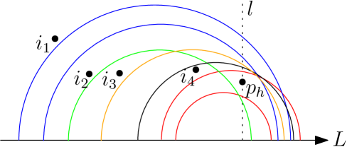
Figure 13: Illustrating the processing of an event at $p_{h}\in P$: $(i_{2},h)$ and $(i_{4},h)$ will be reported as middle bounding couples, point $i_{2}$ will be removed from $P(l)$ and $p_{h}$ will be inserted to $P(l)$.

The above discusses the case where $p_{h}$ is above $s_{k}$. If $p_{h}$ is not above $s_{k}$, then we are done with processing the arcs of $H^{*}$. We can show that all middle bounding couples $(b,h)$ with $h$ as the right end have been computed. The proof is similar to Lemma 17, and we omit the details.

Finally, we add $p_{h}$ to the rear of $P(l)$. As in the $L_{\infty}$ case, we need to compute the tree $T(H(h))$ for the set $H(h)$, which is comprised of all arcs of $H$ below $p_{h}$, as follows.

Initially we have an empty tree $T(H(h))$. Let $H^{\prime}$ be the subset of the arcs of $H^{*}$ vertically below $p_{h}$; here $H^{*}$ refers to the original set at the beginning of the event for $p_{h}$. The set $H^{\prime}$ has already been computed above. Let $\mathcal{H}^{\prime}$ be the subcollection of $\mathcal{H}$ whose lowest arcs are in $H^{\prime}$. We process the subsets $H(i_{j})$ of $\mathcal{H}^{\prime}$ in the inverse order of their indices (for this, after identifying $\mathcal{H}^{\prime}$, we can sort the subsets $H(i_{j})$ of $\mathcal{H}^{\prime}$ by their indices in $O(|H^{\prime}|\log m)$ time; note that $|H^{\prime}|=|\mathcal{H}^{\prime}|$), i.e., the subset of $\mathcal{H}^{\prime}$ with the largest index is processed first.

Suppose we are processing a subset $H(i_{j})$ of $\mathcal{H}^{\prime}$. Let $s$ be the lowest arc of $H(i_{j})$. Recall that we have performed a split operation on the tree $T(H(i_{j}))$ to obtain another tree consisting of all arcs of $H(i_{j})$ below $p_{h}$, and we use $H^{\prime}(i_{j})$ to denote the set of those arcs and use $T(H^{\prime}(i_{j}))$ to denote the tree. If $T(H(h))$ is empty, then we simply set $T(H(h))=T(H^{\prime}(i_{j}))$. Otherwise, we find the highest arc $s^{\prime}$ of $T(H(h))$ at $l$. If $s$ is above $s^{\prime}$ at $l$, then every arc of $T(H^{\prime}(i_{j}))$ is above all arcs of $T(H(h))$ at $l$ and thus we simply perform a merge operation to merge $T(H^{\prime}(i_{j}))$ with $T(H(h))$ (and we use $T(H(h))$ to refer to the new merged tree). Otherwise, we call $(s,s^{\prime})$ an order-violation pair. In this case, we do the following. We remove $s$ from $T(H^{\prime}(i_{j}))$ and insert it to $T(H(h))$. If $T(H^{\prime}(i_{j}))$ becomes empty, then we finish processing $H(i_{j})$. Otherwise, we find the new lowest arc of $T(H^{\prime}(i_{j}))$, still denoted by $s$, and then process $s$ in the same way as above.

The above describes our algorithm for processing a subset $H(i_{j})$ of $\mathcal{H}^{\prime}$. Once all subsets of $\mathcal{H}^{\prime}$ are processed, the tree $T(H(h))$ for the set $H(h)$ is obtained.

After processing the arcs of $H^{*}$ as above, we also need to consider the arcs of $H(i_{0})$. For this, we simply scan the arcs from low to high using the tree $T(H(i_{0}))$, and for each arc $s$, if $s$ is above $p_{h}$, then we stop the procedure; otherwise, we remove $s$ from $T(H(i_{0}))$ and insert it to $T(H(h))$.

This finishes our algorithm for processing the event at $p_{h}$. The runtime of this step is $O((1+k_{1}+k_{2}+k_{3})\cdot\log m)$ time, where $k_{1}$ is the number of middle bounding couples reported (the number of merge and split operations is at most $k_{1}$; also, $|H^{\prime}|=k_{1}$), $k_{2}$ is the number of arcs of $H(i_{0})$ got removed for constructing $T(H(h))$, and $k_{3}$ is the number of order-violation pairs. By Lemma 18, the total sum of $k_{1}$ is at most $2(n+m)+\kappa$ in the entire algorithm. As in the $L_{\infty}$ case, the total sum of $k_{2}$ is at most $m$ in the entire algorithm. The following lemma proves that the total sum of $k_{3}$ is at most $\kappa$. Therefore, the overall time of the algorithm is $O((n+m)\log(n+m)+\kappa\log m)$.

Lemma 20

The total number of order-violation pairs in the entire algorithm is at most $\kappa$.

Proof

We follow the notation defined above. Consider an order-violation pair $(s,s^{\prime})$, which appears when we process a subset $H^{\prime}(i_{j})$ of $\mathcal{H}^{\prime}$ for constructing $T(H(h))$ during an event at a point $p_{h}\in P$, such that $s\in H^{\prime}(i_{j})$ and $s^{\prime}\in T(H(h))$. Without loss of generality, we assume that this is the first time that $(s,s^{\prime})$ appears as an order-violation pair in our entire algorithm. As we process the subsets of $\mathcal{H}^{\prime}$ by their inverse index order, $s^{\prime}$ is from $H(i_{k})$ for some $k$ with $j<k\leq t$. Since $(s,s^{\prime})$ is an order-violation pair, by definition, $s^{\prime}$ is strictly above $s$ at $x(l)=x(p_{h})$; e.g., see Fig. 14. On the other hand, since $s^{\prime}\in H(i_{k})$, we know that $p_{i_{k}}$ is vertically above $s^{\prime}$. Since $s\in H(i_{j})$ with $j<k$, $p_{i_{k}}$ must be vertically below $s$. Thus, $s$ is strictly above $s^{\prime}$ at $x(p_{i_{k}})$. This implies that $s$ and $s^{\prime}$ has an intersection strictly between $p_{i_{k}}$ and $p_{h}$. We charge the pair $(s,s^{\prime})$ to that intersection. Because $s$ and $s^{\prime}$ can have only one intersection, in the following we show that $(s,s^{\prime})$ will never appear as an order-violation pair again in the future algorithm.

Figure 14: Illustrating the proof of Lemma 20: the point $i_{k}$ is vertically below $s$ but vertically above $s^{\prime}$.

First of all, according to our algorithm, $(s,s^{\prime})$ will not appear as an order-violation pair again during processing the event at $p_{h}$. After the event, both $s$ and $s^{\prime}$ are in $H(h)$. Consider a future event for processing another point $p_{h^{\prime}}\in P$. By our algorithm invariant (2), we have a collection $\mathcal{H}$ of sets $H_{i^{\prime}_{j}}$ with $j=0,1,\ldots,t^{\prime}$. Assume to the contrary that $(s,s^{\prime})$ appears as an order-violation pair again. Then, $s$ and $s^{\prime}$ must be from two different sets of $\mathcal{H}$, e.g., $H_{i^{\prime}_{j}}$ and $H_{i^{\prime}_{k}}$. Without loss of generality, let $j<k$. By the same analysis as before, we can obtain that $s$ and $s^{\prime}$ have an intersection $q$ strictly between $p_{i^{\prime}_{j}}$ and $p_{h^{\prime}}$. Since both $s$ and $s^{\prime}$ were in $H(h)$ right after the event at $p_{h}$, it must hold that $x(p_{h})\leq x(p_{i^{\prime}_{j}})$. Hence, $x(p_{h})<x(q)$. But this incurs contradiction because we have shown before that the only intersection between $s$ and $s^{\prime}$ is strictly to the left of $p_{h}$.

The above shows that $(s,s^{\prime})$ will appear as an order-violation pair exactly once in the entire algorithm, which is charged to their only intersection. Therefore, the total number of order-violation pairs in the entire algorithm is at most $\kappa$. ∎

In summary, all middle bounding couples of $\mathcal{C}$ can be computed in $O((n+m)\log(n+m)+\kappa\log m)$ time. Combining with Lemmas 18 and 19, Lemma 11 is proved.

7 The line-separable unit-disk coverage and the half-plane coverage

In this section, we show that our techniques for the line-constrained disk coverage problems can also be used to solve other geometric coverage problems.

Recall that the line-separable unit-disk coverage problem refers to the case in which $P$ and centers of $S$ are separated by a line $\ell$ and all disks of $S$ have the same radius. Without loss of generality, we assume that $\ell$ is the $x$-axis and all points of $P$ are above $\ell$. Hence, for each disk $s_{i}$ of $S$, the portion of $s_{i}$ above $\ell$ is a subset of its upper half disk. Since disks of $S$ have the same radius, the boundaries of any two disks intersect at most once above $\ell$. We define $\kappa$ as the number of pairs of disks that intersect above $\ell$. Due to the above properties, to solve the problem, we can simply use the same algorithm in Section 6 for the line-constrained $L_{2}$ case. Indeed, one can verify that the following critical lemmas that the algorithm relies on still hold: Lemmas 5, 6, 18, 19, and 20. By Theorem 6.2, we obtain the following.

Theorem 7.1

Given in the plane a set $P$ of $n$ points and a set $S$ of $m$ weighted unit-disks such that $P$ and centers of disks $S$ are separated by a line $\ell$, one can compute a minimum weight disk coverage for $P$ in $O(nm\log(m+n))$ time or in $O((n+m)\log(n+m)+\kappa\log m)$ time, where $\kappa$ is the number of pairs of disks of $S$ that intersect in the side of $\ell$ containing $P$.

Remark.

Note that although disks of $S$ have the same radius, because their centers may not be on the same line, one can verify that Lemma 1 does not hold any more. Hence, we can not use the same algorithm as in Section 4 for the line-constrained unit-disk case. But if the centers of all disks of $S$ lie on the same line parallel to $\ell$ (and below $\ell$), then Lemma 1 will hold and thus we can use the same algorithm as in Section 4 to solve the problem in $O((n+m)\log(n+m))$ time.

We now consider the half-plane coverage problem. Given in the plane a set $P$ of $n$ points and a set $S$ of weighted half-planes, the goal is compute a minimum weight half-plane coverage for $P$, i.e., compute a subset of half-planes to cover all points of $P$ so that the total sum of the weights of the half-planes in the subset is minimized.

We start with the lower-only case where all half-planes of $S$ are lower ones. The problem can be reduced to the line-separable unit-disk coverage problem. Indeed, we first find a horizontal line $\ell$ below all points of $P$. Then, since each half-plane $h$ of $S$ is a lower one, $h$ can be considered as a disk of infinite radius with center below $\ell$. In this way, $S$ becomes a set of unit-disks whose centers are below $\ell$. By Theorem 7.1, we have the following result.

Theorem 7.2

Given in the plane a set $P$ of $n$ points and a set $S$ of $m$ weighted lower half-planes, one can compute a minimum weight half-plane coverage for $P$ in $O(nm\log(m+n))$ time or in $O(n\log n+m^{2}\log m)$ time.

For the general case where $S$ may contain both lower and upper half-planes, we reduce it to a set of $O(n^{2})$ instances of the lower-only case, as follows.

Let $S_{opt}$ denote the subset of $S$ in an optimal solution. Har-Peled and Lee [13] observed that if the half-planes of $S_{opt}$ together cover the entire plane then the size of $S_{opt}$ is $3$; in this case, we can enumerate all triples of $S$ and thus obtain an optimal solution in $O(n^{3})$ time.

In the following we consider the case where the union of the half-planes of $S_{opt}$ does not cover the entire plane. In this case, the complement of the union of the half-planes of $S_{opt}$ is a (possibly unbounded) convex polygon $R$ [13]. For the ease of discussion, we assume that $R$ is bounded since the algorithm for the other case is similar. Let $a$ and $b$ refer to the leftmost and rightmost vertices of $R$, respectively. Let $P_{1}$ denote the subset of points of $P$ below the line through $a$ and $b$, and $P_{2}=P\setminus P_{1}$. The two vertices $a$ and $b$ together partition the edges of $R$ into two chains, a lower chain and an upper chain. Observe that the half-planes that are bounded by the supporting lines of the edges in the lower chain are all lower half-planes and they together cover $P_{1}$; similarly, the half-planes that are bounded by the supporting lines of the edges of the upper chain are all upper half-planes and they together cover $P_{2}$. In light of the observation, finding a minimum weight coverage for $P$ is equivalent to solving the following two lower-only case sub-problems: finding a minimum weight coverage for $P_{1}$ using lower half-planes of $S$ and finding a minimum weight coverage for $P_{2}$ using upper half-planes of $S$. Because we do not know $P_{1}$ and $P_{2}$, we enumerate all possible partitions of $P$ by a line. Clearly, there are $O(n^{2})$ such partitions. Hence, solving the half-plane coverage problem for $P$ and $S$ is reduced to $O(n^{2})$ instances of the lower-only case. By Theorem 7.2, we can obtain the following result.

Theorem 7.3

Given in the plane a set $P$ of $n$ points and a set $S$ of $m$ weighted half-planes, one can compute a minimum weight half-plane coverage for $P$ in $O(n^{3}m\log(m+n))$ time or in $O(n^{3}\log n+n^{2}m^{2}\log m)$ time.

8 Concluding remarks

We show that our line-constrained disk coverage problem has an $\Omega((m+n)\log(m+n))$ time lower bound in the algebraic decision tree model even for the 1D case. To this end, in the following we prove that $\Omega(N\log N)$ is a lower bound with $N=\max\{m,n\}$, which implies the $\Omega((m+n)\log(m+n))$ lower bound as $N=\Theta(n+m)$.

The reduction is from the element uniqueness problem. Let $X=\{x_{1},x_{2},\ldots,x_{n}\}$ be a set of $n$ numbers, as an instance of the element uniqueness problem. We create an instance of the 1D disk coverage problem with a point set $P$ and a segment set $S$ on the $x$-axis $L$ as follows. For each $x_{i}\in X$, we create a point on $L$ with $x$-coordinate equal to $x_{i}$ and create a segment on $L$ which is the above point with weight equal to $1$. Let $P$ be the set of all such points and let $S$ be the set of all such segments. Then, $|P|=|S|=n$, and thus $N=n$. It is not difficult to see that the numbers of $X$ are distinct if and only if the optimal objective value of the 1D disk coverage problem is equal to $n$. As the element uniqueness problem has an $\Omega(n\log n)$ time lower bound under the algebraic decision tree model, our 1D disk coverage problem has an $\Omega(N\log N)$ time lower bound.

The lower bound implies that our algorithms for the 1D, unit-disk, $L_{1}$, and $L_{\infty}$ cases are all optimal. However, it remains open whether faster algorithms exist for the $L_{2}$ case. Another direction is to investigate whether the $L_{2}$ case is 3SUM-hard; if yes, then it is quite likely that our algorithm is nearly optimal.

References

- [1] H. Alt, E.M. Arkin, H. Brönnimann, J. Erickson, S.P. Fekete, C. Knauer, J. Lenchner, J.S.B. Mitchell, and K. Whittlesey. Minimum-cost coverage of point sets by disks. In Proceedings of the 22nd Annual Symposium on Computational Geometry (SoCG), pages 449–458, 2006.
- [2] C. Ambühl, T. Erlebach, M. Mihalák, and M. Nunkesser. Constant-factor approximation for minimum-weight (connected) dominating sets in unit disk graphs. In Proceedings of the 9th International Conference on Approximation Algorithms for Combinatorial Optimization Problems (APPROX), and the 10th International Conference on Randomization and Computation (RANDOM), pages 3–14, 2006.
- [3] J.L. Bentley and T.A. Ottmann. Algorithms for reporting and counting geometric intersections. IEEE Transactions on Computers, 28(9):643–647, 1979.
- [4] V. Bilò, I. Caragiannis, C. Kaklamanis, and P. Kanellopoulos. Geometric clustering to minimize the sum of cluster sizes. In Proceedings of the 13th European Symposium on Algorithms, pages 460–471, 2005.
- [5] A. Biniaz, P. Bose, P. Carmi, A. Maheshwari, I. Munro, and M. Smid. Faster algorithms for some optimization problems on collinear points. In Proceedings of the 34th International Symposium on Computational Geometry (SoCG), pages 8:1–8:14, 2018.
- [6] K.Q. Brown. Comments on “Algorithms for reporting and counting geometric intersections”. IEEE Transactions on Computers, 30:147–148, 1981.
- [7] T.M. Chan and E. Grant. Exact algorithms and APX-hardness results for geometric packing and covering problems. Computational Geometry: Theory and Applications, 47:112–124, 2014.
- [8] F. Claude, G.K. Das, R. Dorrigiv, S. Durocher, R. Fraser, A. López-Ortiz, B.G. Nickerson, and A. Salinger. An improved line-separable algorithm for discrete unit disk cover. Discrete Mathematics, Algorithms and Applications, 2:77–88, 2010.
- [9] F. Claude, R. Dorrigiv, S. Durocher, R. Fraser, A. López-Ortiz, and A. Salinger. Practical discrete unit disk cover using an exact line-separable algorithm. In Proceedings of the 20th International Symposium on Algorithm and Computation (ISAAC), pages 45–54, 2009.
- [10] M. de Berg, O. Cheong, M. van Kreveld, and M. Overmars. Computational Geometry — Algorithms and Applications. Springer-Verlag, Berlin, 3rd edition, 2008.
- [11] T. Feder and D.H. Greene. Optimal algorithms for approximate clustering. In Proceedings of the 20th Annual ACM Symposium on Theory of Computing (STOC), pages 434–444, 1988.
- [12] U. Feige. A threshold of ln n for approximating set cover. Journal of the ACM, 45:634–652, 1998.
- [13] S. Har-Peled and M. Lee. Weighted geometric set cover problems revisited. Journal of Computational Geometry, 3:65–85, 2012.
- [14] D.S. Hochbaum and W. Maass. Fast approximation algorithms for a nonconvex covering problem. Journal of Algorithms, 3:305–323, 1987.
- [15] A. Karmakar, S. Das, S.C. Nandy, and B.K. Bhattacharya. Some variations on constrained minimum enclosing circle problem. Journal of Combinatorial Optimization, 25(2):176–190, 2013.
- [16] N. Lev-Tov and D. Peleg. Polynomial time approximation schemes for base station coverage with minimum total radii. Computer Networks, 47:489–501, 2005.
- [17] J. Li and Y. Jin. A PTAS for the weighted unit disk cover problem. In Proceedings of the 42nd International Colloquium on Automata, Languages and Programming (ICALP), pages 898–909, 2015.
- [18] C. Lund and M. Yannakakis. On the hardness of approximating minimization problems. Journal of the ACM, 41:960–981, 1994.
- [19] N.H. Mustafa and S. Ray. PTAS for geometric hitting set problems via local search. In Proceedings of the 25th Annual Symposium on Computational Geometry (SoCG), pages 17–22, 2009.
- [20] L. Pedersen and H. Wang. On the coverage of points in the plane by disks centered at a line. In Proceedings of the 30th Canadian Conference on Computational Geometry (CCCG), pages 158–164, 2018.
- [21] H. Wang and J. Zhang. Line-constrained -median, -means, and -center problems in the plane. International Journal of Computational Geometry and Application, 26:185–210, 2016.