Molecular vibrational frequencies from analytic Hessian of constrained nuclear-electronic orbital density functional theory

Abstract

Nuclear quantum effects are important in a variety of chemical and biological processes. The constrained nuclear-electronic orbital density functional theory (cNEO-DFT) has been developed to include nuclear quantum effects in energy surfaces. Herein we develop the analytic Hessian for cNEO-DFT energy with respect to the change of nuclear (expectation) positions, which can be used to characterize stationary points on energy surfaces and compute molecular vibrational frequencies. This is achieved by constructing and solving the multicomponent cNEO coupled-perturbed Kohn-Sham (cNEO-CPKS) equations, which describe the response of electronic and nuclear orbitals to the displacement of nuclear (expectation) positions. With the analytic Hessian, the vibrational frequencies of a series of small molecules are calculated and compared to those from conventional DFT Hessian calculations as well as those from the vibrational second-order perturbation theory (VPT2). It is found that even with a harmonic treatment, cNEO-DFT significantly outperforms DFT and is comparable to DFT-VPT2 in the description of vibrational frequencies in regular polyatomic molecules. Furthermore, cNEO-DFT can reasonably describe the proton transfer modes in systems with a shared proton, whereas DFT-VPT2 often faces great challenges. Our results suggest the importance of nuclear quantum effects in molecular vibrations, and cNEO-DFT is an accurate and inexpensive method to describe molecular vibrations.

I Introduction

Multicomponent quantum theory has been an emerging research field in quantum chemistry.(Kreibich and Gross, 2001; Bochevarov et al., 2004; Nakai, 2007; Ishimoto et al., 2009; Abedi et al., 2010; Pavošević et al., 2020) It simultaneously treats at least two types of particles, such as electrons and nuclei, quantum-mechanically and avoids the conventional Born-Oppenheimer (BO) approximation between electrons and nuclei. Thereby, the nuclear quantum effects, which are crucial in many hydrogen-bonded systems such as water,(Ceriotti et al., 2016; Guo et al., 2017) can be described together with electronic quantum effects. The nuclear-electronic orbital (NEO) framework(Webb et al., 2002; Pavošević et al., 2020) is a simple and popular type of multicomponent quantum theory. It simultaneously treats electrons and key nuclei, typically protons, within the orbital picture. In the NEO framework, both wave-function-based methods and density functional theory have been developed, and they have been successful in describing the ground and excited state properties of many small molecules.(Pavošević et al., 2020) However, in conventional NEO calculations, at least two nuclei have to be treated classically to fix the molecular frame and avoid the problems related to translations and rotations.(Iordanov and Hammes-Schiffer, 2003) This practice introduces a new BO separation between the classical and quantum nuclei, which assumes the quantum nuclei respond instantaneously to the motion of classical nuclei. It makes neither the vibrational excitations from NEO time-dependent density functional theory (NEO-TDDFT) nor the normal modes from NEO Hessian directly correspond to the vibrations observed in experiments.(Iordanov and Hammes-Schiffer, 2003; Yang et al., 2018, 2019; Schneider et al., 2021)

Recently, we developed constrained NEO-DFT (cNEO-DFT) to overcome the challenge. In cNEO-DFT, we introduce constraints on the expectation values of the quantum nuclear positions and minimize the total energy under the constraints. These constrained expectation positions naturally fix the molecular frame and therefore enable a full-quantum treatment of molecules. The full-quantum treatment avoids any BO approximation.(Xu and Yang, 2020a) In cNEO theory, the energy surface is a function of the quantum nuclear expectation positions as well as the classical nuclear positions.(Xu and Yang, 2020b) This is similar to BO potential energy surface, but because quantum nuclei are described by orbitals rather than fixed point charges, the cNEO energy surfaces incorporate nuclear quantum effects, in particular the zero-point effects. Previously, we have successfully performed geometry optimizations and transition states search on the cNEO energy surfaces for several simple molecular systems and chemical reactions.(Xu and Yang, 2020a) The zero-point effects and geometric isotope effects have been observed on the cNEO surface, suggesting the promising future of cNEO-DFT in describing systems and reactions with significant nuclear quantum effects. However, the characterization of reactants, products, and transition states on the cNEO surface is needed when applying cNEO theory to practical quantum chemistry calculations, which requires the computation of the Hessian of cNEO energies. In this work, we will derive and implement the analytic Hessian for cNEO energies and investigate its performance through molecular vibrational frequency calculations.

The Hessian can be obtained either numerically or analytically. However, the numerical Hessian is often more expensive and can suffer from the amplification of numerical error or the contamination of higher-order terms.(Pulay, 2014) In contrast, analytic Hessian has higher computational efficiency and numerical accuracy.(Pulay, 2014) In conventional electronic structure theory, the calculation of analytic Hessian requires the response of the electronic orbitals to the perturbative nuclear displacement, which can be obtained by solving coupled perturbed Hartree-Fock/Kohn-Sham equations.(Pople et al., 1979; Pulay, 1983; Komornicki and Fitzgerald, 1993; Yamaguchi and Schaefer III, 2011) In cNEO-DFT, the analytic Hessian requires the response of both electronic and nuclear orbitals to the perturbative change in quantum nuclear expectation positions as well as classical nuclear positions. It requires solving a multicomponent cNEO coupled perturbed Kohn-Sham (cNEO-CPKS) equation, which couples the response of electrons and quantum nuclei. In addition, the constraints in nuclear expectation positions lead to additional terms incorporated in the cNEO-CPKS equation.

The rest of the paper is organized as follows. In Sec. II, we present the expression of analytic Hessian for cNEO-DFT as well as the formulation of cNEO-CPKS equations. Then we investigate the vibrational frequencies of a series of molecules by building and diagonalizing the cNEO Hessian matrices, with the computational details presented in Sec III and results presented in Sec IV. The performance of cNEO-DFT is further compared with other commonly used methods, including harmonic DFT, DFT-VPT2, and NEO-DFT(V). We give our concluding remarks in Sec V.

II Theory

II.1 Energy and derivatives

In cNEO-DFT, the electrons can be treated in the same way as in conventional DFT, whereas quantum nuclei are treated as distinguishable particles because they are relatively localized in space.(Xu and Yang, 2020b, a) The total energy can be written as

$$E =\sum_{i}h_{ii}+\frac{1}{2}\sum_{ij}(ii|jj)+\sum_{n}h_{I_{n}I_{n}}+\frac{1}{2}\sum_{n,n^{\prime}}Z_{n}Z_{n^{\prime}}(I_{n}I_{n}|I_{n^{\prime}}I_{n^{\prime}})-\sum_{n}\sum_{i}Z_{n}(ii|I_{n}I_{n})$$

$$+E^{\text{xc}}[\rho^{e},\{\rho^{n}\}]+\frac{1}{2}\sum_{A}\sum_{B\neq A}\frac{Z_{A}Z_{B}}{|\mathbf{R}_{A}-\mathbf{R}_{B}|},$$ (1)

where each term represents the core Hamiltonian for electrons, the electronic Coulomb interaction, the core Hamiltonian for nuclei, the nuclear Coulomb interaction, the electron-nuclear Coulomb interaction, the exchange-correlation energy as a functional of both electronic density $\rho^{e}$ and nuclear densities $\{\rho^{n}\}$, and the Coulomb repulsion between classical nuclei. In this paper, we will use $i,j,k,l$ to denote occupied molecular orbitals, $a,b,c,d$ to denote unoccupied molecular orbitals, and $p,q,r,s,m$ to denote general molecular orbitals. We will use the corresponding upper case letters to denote nuclear orbitals. Because quantum nuclei are treated as distinguishable particles, each nucleus occupies one orbital and we use $I_{n}$ ( or $J_{n}$, $K_{n}$) to denote the only occupied orbital for the $n$th quantum nucleus. We will use $\mu,\nu$ to denote electronic atomic orbitals and $\mu_{n},\nu_{n}$ to denote the atomic orbitals for the $n$th quantum nucleus. The exchange-correlation energy $E^{\text{xc}}$ includes electronic exchange-correlation, nuclear exchange-correlation, and electronic-nuclear correlation. The definition of the two-particle integral is

$$(ij|kl)=\int\phi_{i}(\mathbf{r}^{\prime})\phi_{j}(\mathbf{r}^{\prime})\frac{1}{|\mathbf{r}-\mathbf{r}^{\prime}|}\phi_{k}(\mathbf{r})\phi_{l}(\mathbf{\mathbf{r}})\mathrm{d}\mathbf{r}^{\prime}\mathrm{d}\mathbf{r}.$$ (2)

The constraint on the expectation position of the $n$th quantum nucleus is

$$\mathbf{r}_{I_{n}I_{n}}\equiv(I_{n}|\mathbf{r}|I_{n})\equiv\int\phi_{I_{n}}(\mathbf{r})\mathbf{r}\phi_{I_{n}}(\mathbf{\mathbf{r}})\mathrm{d}\mathbf{r}=\mathbf{R}_{n},$$ (3)

and the additional term in the Lagrangian for the constraint is

$$\sum_{n}\mathbf{f}_{n}\cdot(\mathbf{r}_{I_{n}I_{n}}-\mathbf{R}_{n}),$$ (4)

where $\mathbf{f}_{n}$ is the Lagrange multiplier for the $n$th quantum nucleus, and it has been proven to be the classical force acting on the nucleus in the complete basis set limit.(Xu and Yang, 2020b)

Minimizing the Lagrangian with respect to electronic and nuclear densities leads to the Fock equations, and the electronic and nuclear Fock matrix elements are defined as

$$F_{pq}=h_{pq}+\sum_{k}(pq|kk)-\sum_{n}Z_{n}(pq|I_{n}I_{n})+V_{pq}^{\text{xc}},$$ (5)

and

$$F_{P_{n}Q_{n}}=h_{P_{n}Q_{n}}-\sum_{k}Z_{n}(P_{n}Q_{n}|kk)+\sum_{n^{\prime}}Z_{n}Z_{n^{\prime}}(P_{n}Q_{n}|I_{n^{\prime}}I_{n^{\prime}})+V_{P_{n}Q_{n}}^{\text{xc}}+\mathbf{f}_{n}\cdot(P_{n}|\mathbf{r}|Q_{n}),$$ (6)

respectively, where $V^{\text{xc}}$ is the exchange-correlation potential for either electrons or nuclei depending on the subscripts.

The gradient and Hessian of the energy requires the computation of the derivatives for some key components, including $h_{ii}$, $(ii|jj)$, $h_{I_{n}I_{n}}$, $(I_{n}I_{n}|I_{n^{\prime}}I_{n^{\prime}})$, $(ii|I_{n}I_{n})$, $E^{\text{xc}}[\rho^{e},\{\rho^{n}\}]$, which can be obtained analogously to conventional electronic Hartree-Fock and Kohn-Sham DFT. The detailed derivation for the required terms are presented in the Supplementary Materials. However, unlike conventional theories with only constraints on orbital normalization, cNEO-DFT additionally imposes the constraints on nuclear expectation positions and therefore requires the derivative of the constraints in the derivation of gradient and Hessian. The derivative of the constraint (Eq. 3) with respect to a perturbation $\xi$ is

$$\frac{\partial\mathbf{R}_{n}}{\partial\xi}=\mathbf{r}_{I_{n}I_{n}}^{\xi}+\sum_{M_{n}}(\mathbf{r}_{I_{n}M_{n}}U_{M_{n}I_{n}}^{\xi}+U_{M_{n}I_{n}}^{\xi}\mathbf{r}_{M_{n}I_{n}}),$$ (7)

where the matrix $\mathbf{U}^{\xi}$ follows the same definition as Ref. Yamaguchi and Schaefer III, 2011 and describes the response of the molecular orbital coefficient matrix $\mathbf{C}$ to the perturbation $\xi$: ,

$$\frac{\partial C_{\mu_{n}P_{n}}}{\partial\xi} =\sum_{M_{n}}C_{\mu_{n}M_{n}}U_{M_{n}P_{n}}^{\xi},$$ (8)

where $\mathbf{r}_{I_{n}I_{n}}^{\xi}$ is defined as

$$\mathbf{r}_{I_{n}I_{n}}^{\xi}=\sum_{\mu_{n}\nu_{n}}C_{\mu_{n}I_{n}}C_{\nu_{n}I_{n}}\frac{\partial\mathbf{r}_{\mu_{n}\nu_{n}}}{\partial\xi}.$$ (9)

The first-order derivative for the total energy is

$$\frac{\partial E}{\partial\xi} =\sum_{i}h_{ii}^{\xi}+\frac{1}{2}\sum_{ij}(ii|jj)^{\xi}+\sum_{n}h_{I_{n}I_{n}}^{\xi}-\sum_{n}\sum_{i}Z_{n}(ii|I_{n}I_{n})^{\xi}+\frac{1}{2}\sum_{n,n^{\prime}}Z_{n}Z_{n^{\prime}}(I_{n}I_{n}|I_{n^{\prime}}I_{n^{\prime}})^{\xi}$$

$$+\sum_{i}V_{ii}^{\text{\text{xc}},\xi}+\sum_{n}V_{I_{n}I_{n}}^{\text{xc},\xi}-\sum_{i}\epsilon_{i}S_{ii}^{\xi}-\sum_{n}\epsilon_{I_{n}}S_{I_{n}I_{n}}^{\xi}+\sum_{n}\mathbf{f}_{n}\cdot\mathbf{r}_{I_{n}I_{n}}^{\xi}-\sum_{n}\mathbf{f}_{n}\cdot\frac{\partial\mathbf{R}_{n}}{\partial\xi},$$ (10)

where $\epsilon$ is the orbital energy, $S$ is the overlap matrix, and quantities with the superscript $\xi$ are partial derivatives defined analogously to Eq. 9 in which the molecular orbital coefficients $\mathbf{C}$ is not differentiated. When $\xi$ is chosen to be the expectation position of a particular quantum nucleus $\xi=\mathbf{R}_{n_{0}}$, this expression is the same as the gradient result in our previous work,(Xu and Yang, 2020a) with the last term being

$$-\sum_{n}\mathbf{f}_{n}\cdot\frac{\partial\mathbf{R}_{n}}{\partial\mathbf{R}_{n_{0}}}=-\mathbf{f}_{n_{0}}.$$ (11)

The second-order derivative for the total energy can be obtained by taking the derivative of Eq. 10 with respect to another perturbation $\chi$. The final expression is

$$\frac{\partial^{2}E}{\partial\xi\partial\chi} =\sum_{i}h_{ii}^{\xi\chi}+\frac{1}{2}\sum_{ij}(ii|jj)^{\xi\chi}+\sum_{n}h_{I_{n}I_{n}}^{\xi\chi}-\sum_{i,n}Z_{n}(ii|I_{n}I_{n})^{\xi\chi}+\frac{1}{2}\sum_{n,n^{\prime}}Z_{n}Z_{n^{\prime}}(I_{n}I_{n}|I_{n^{\prime}}I_{n^{\prime}})^{\xi\chi}$$

$$+\sum_{i}V_{ii}^{\text{xc},\xi\chi}+\sum_{n}V_{I_{n}I_{n}}^{\text{xc},\xi\chi}$$

$$+\sum_{ik}K_{(ii)^{\xi},(kk)^{\chi}}^{\text{xc}}+\sum_{in}K_{(ii)^{\xi},(K_{n}K_{n})^{\chi}}^{\text{xc}}+\sum_{nn^{\prime}}K_{(I_{n}I_{n})^{\xi},(K_{n^{\prime}}K_{n^{\prime}})^{\chi}}^{\text{xc}}+\sum_{nk}K_{(I_{n}I_{n})^{\xi},(kk)^{\chi}}^{\text{xc}}$$

$$+2\sum_{i}\sum_{p}(F_{ip}^{\xi}U_{pi}^{\chi}+F_{ip}^{\chi}U_{pi}^{\xi})+2\sum_{n}\sum_{P_{n}}(F_{I_{n}P_{n}}^{\xi}U_{P_{n}I_{n}}^{\chi}+F_{I_{n}P_{n}}^{\chi}U_{P_{n}I_{n}}^{\xi})-\sum_{i}\epsilon_{i}S_{ii}^{\xi\chi}-\sum_{n}\epsilon_{I_{n}}S_{I_{n}I_{n}}^{\xi\chi}$$

$$+2\sum_{i}\sum_{p}U_{pi}^{\chi}U_{pi}^{\xi}\epsilon_{p}+2\sum_{n}\sum_{P_{n}}U_{P_{n}I_{n}}^{\chi}U_{P_{n}I_{n}}^{\xi}\epsilon_{P_{n}}$$

$$-2\sum_{i}\sum_{p}\epsilon_{i}(U_{ip}^{\chi}U_{ip}^{\xi}-S_{ip}^{\xi}S_{pi}^{\chi})-2\sum_{n}\sum_{P_{n}}\epsilon_{I_{n}}(U_{I_{n}P_{n}}^{\chi}U_{I_{n}P_{n}}^{\xi}-S_{I_{n}P_{n}}^{\xi}S_{P_{n}I_{n}}^{\chi})$$

$$+2\sum_{i}\sum_{p}[\sum_{k}\sum_{q}(2(ip|kq)+2K_{ip,kq}^{\text{xc}})U_{qk}^{\chi}U_{pi}^{\xi}-\sum_{n}\sum_{P_{n}}2(Z_{n}(ip|K_{n}P_{n})-K_{ip,K_{n}P_{n}}^{\text{xc}})U_{P_{n}K_{n}}^{\chi}U_{pi}^{\xi}]$$

$$+2\sum_{n}\sum_{P_{n}}[\sum_{n^{\prime}}\sum_{Q_{n^{\prime}}}(2Z_{n}Z_{n^{\prime}}(I_{n}P_{n}|K_{n^{\prime}}Q_{n^{\prime}})+2K_{I_{n}P_{n},K_{n^{\prime}}Q_{n^{\prime}}}^{\text{xc}})U_{Q_{n^{\prime}}K_{n^{\prime}}}^{\chi}U_{P_{n}I_{n}}^{\xi}$$

$$-\sum_{k}\sum_{p}2(Z_{n}(I_{n}P_{n}|kp)-K_{I_{n}P_{n},kp}^{\text{xc}})U_{pk}^{\chi}U_{P_{n}I_{n}}^{\xi}]$$

$$+\sum_{n}\mathbf{f}_{n}\cdot\mathbf{r}_{I_{n}I_{n}}^{\xi\chi}-\mathbf{f}_{n}\cdot\frac{\partial^{2}\mathbf{R}_{n}}{\partial\xi\partial\chi},$$ (12)

where $K^{\text{xc}}$ is the exchange-correlation kernel and the detailed derivation for the equation is provided in Supporting Information. The key components in the expression can be calculated analogously to conventional electronic CPKS. The knowledge of $\mathbf{U}$ can be obtained by solving the cNEO-CPKS equation, which will be presented in next section. Note that when $\xi$ and $\chi$ are both chosen to be the nuclear expectation positions, the last term $-\mathbf{f}_{n}\cdot\frac{\partial^{2}\mathbf{R}_{n}}{\partial\xi\partial\chi}$ vanishes.

II.2 cNEO-CPKS

As with conventional electronic DFT, a converged SCF solution for cNEO-DFT always satisfies $F_{ia}=0$, which leads to

$$\frac{\partial F_{ai}}{\partial\xi}=0.$$ (13)

We can calculate the derivative of electronic Fock matrix elements in a similar way to conventional electronic DFT, but with additional Coulomb and correlation terms from nuclei.

$$0= \frac{\partial F_{ai}}{\partial\xi}$$ (14)

$$= F_{ai}^{\xi}+(\epsilon_{a}-\epsilon_{i})U_{ai}^{\xi}-S_{ai}^{\xi}\epsilon_{i}+2\sum_{jb}((ai|bj)+K_{ai,bj}^{\text{xc}})U_{bj}^{\xi}-2\sum_{n}\sum_{B_{n}}(Z_{n}(ai|B_{n}J_{n})-K_{ai,B_{n}J_{n}}^{\text{xc}})U_{B_{n}J_{n}}^{\xi}$$

$$-\sum_{jk}((ai|kj)+K_{ai,kj}^{\text{xc}})S_{kj}^{\xi}+\sum_{n}(Z_{n}(ai|J_{n}J_{n})-K_{ai,J_{n}J_{n}}^{\text{xc}})S_{J_{n}J_{n}}^{\xi}.$$

Analogously, the derivative of the nuclear Fock matrix can be derived. The difference is that the extra Lagrange multiplier term in the nuclear Fock matrix (Eq. 6) gives an additional term in its derivative,

$$0= \frac{\partial F_{A_{n}I_{n}}}{\partial\xi}$$ (15)

$$= F_{A_{n}I_{n}}^{\xi}+(\epsilon_{A_{n}}-\epsilon_{I_{n}})U_{A_{n}I_{n}}^{\xi}-S_{A_{n}I_{n}}^{\xi}\epsilon_{I_{n}}$$

$$+2\sum_{n^{\prime}}\sum_{B_{n^{\prime}}}(Z_{n}Z_{n^{\prime}}(A_{n}I_{n}|B_{n^{\prime}}J_{n^{\prime}})+K_{A_{n}I_{n},B_{n^{\prime}}J_{n^{\prime}}}^{\text{xc}})U_{B_{n^{\prime}}J_{n^{\prime}}}^{\xi}-2\sum_{j}\sum_{b}(Z_{n}(A_{n}I_{n}|bj)-K_{A_{n}I_{n},bj}^{\text{xc}})U_{bj}^{\xi}$$

$$-\sum_{n^{\prime}}(Z_{n}Z_{n^{\prime}}(A_{n}I_{n}|J_{n^{\prime}}J_{n^{\prime}})+K_{A_{n}I_{n},J_{n^{\prime}}J_{n^{\prime}}}^{\text{xc}})S_{J_{n^{\prime}}J_{n^{\prime}}}^{\xi}+\sum_{j}\sum_{k}(Z_{n}(A_{n}I_{n}|kj)-K_{A_{n}I_{n},kj}^{\text{xc}})S_{jk}^{\xi}+\frac{\partial\mathbf{f}_{n}}{\partial\xi}\cdot\mathbf{r}_{A_{n}I_{n}}.$$

The unknown variables in Eq. 14 and 15 are the electronic and nuclear $\mathbf{U}^{\xi}$ matrices as well as the derivative of $\mathbf{f}$ with respect to $\xi$. These two sets of equations are not sufficient to solve all unknown variables, and the derivative of the constraint also needs to be included. Rearranging Eq. 7 leads to

$$\sum_{B_{n}}\mathbf{r}_{I_{n}B_{n}}U_{B_{n}I_{n}}^{\xi} =\frac{1}{2}(\frac{\partial\mathbf{R}_{n}}{\partial\xi}-\mathbf{r}_{I_{n}I_{n}}^{\xi}+\mathbf{R}_{n}S_{I_{n}I_{n}}^{\xi}).$$ (16)

Note that here we have used the relationship $2U_{I_{n}I_{n}}^{\xi}=-S_{I_{n}I_{n}}^{\xi}$, which is derived from the derivative of the normalization constraint.(Pople et al., 1979) The three sets of equations Eq. 14, 15 and 16 can be cast into a coupled form, which is the cNEO-CPKS equation,

$$\left[\begin{array}[]{ccc}\mathbf{A}^{ee}&\mathbf{A}^{en}&\mathbf{0}\\ \mathbf{A}^{ne}&\mathbf{A}^{nn}&\mathbf{r}\\ \mathbf{0}&\mathbf{r}&\mathbf{0}\end{array}\right]\left[\begin{array}[]{c}\mathbf{U}^{\xi e}\\ \mathbf{U}^{\xi n}\\ \mathbf{f}^{\xi}\end{array}\right]=\left[\begin{array}[]{c}\mathbf{B}^{e}\\ \mathbf{B}^{n}\\ \mathbf{D}\end{array}\right],$$ (17)

with

$$A_{ia,jb}^{ee} =\delta_{ab}\delta_{ij}(\epsilon_{i}-\epsilon_{a})-(2(ai|bj)+2K_{ai,bj}^{xc}),$$

$$A_{ia,J_{n}B_{n}}^{en} =2(Z_{n}(ai|B_{n}J_{n})-K_{ai,B_{n}J_{n}}^{xc}),$$

$$A_{I_{n}A_{n},jb}^{ne} =2(Z_{n}(A_{n}I_{n}|bj)-K_{A_{n}I_{n},bj}^{xc}),$$

$$A_{I_{n}A_{n},J_{n^{\prime}}B_{n^{\prime}}}^{nn} =\delta_{A_{n}B_{n^{\prime}}}\delta_{I_{n}J_{n^{\prime}}}(\epsilon_{I_{n}}-\epsilon_{A_{n}})-2(Z_{n}Z_{n^{\prime}}(A_{n}I_{n}|B_{n^{\prime}}J_{n^{\prime}})+K_{A_{n}I_{n},J_{n^{\prime}}B_{n^{\prime}}}^{xc}),$$

$$\mathbf{r}_{I_{n}A_{n},J_{n^{\prime}}B_{n^{\prime}}}^{nn} =\delta_{A_{n}B_{n^{\prime}}}\delta_{I_{n}J_{n^{\prime}}}\mathbf{r}_{A_{n}I_{n}},$$

$$B_{ia}^{e} =F_{ai}^{\xi}-S_{ai}^{\xi}\epsilon_{i}-\sum_{j}\sum_{k}((ai|kj)+K_{ai,jk}^{xc})S_{jk}^{\xi}+\sum_{n}(Z_{n}(ai|J_{n}J_{n})-K_{ai,J_{n}J_{n}}^{xc})S_{J_{n}J_{n}}^{\xi},$$

$$B_{I_{n}A_{n}}^{n} =F_{A_{n}I_{n}}^{\xi}-S_{A_{n}I_{n}}^{\xi}\epsilon_{I_{n}}+\sum_{j}\sum_{k}(Z_{n}(A_{n}I_{n}|kj)-K_{A_{n}I_{n},jk}^{xc})S_{jk}^{\xi},$$

$$\mathbf{D}_{n} =\frac{1}{2}(\frac{\partial\mathbf{R}_{n}}{\partial\xi}-\mathbf{r}_{I_{n}I_{n}}^{\xi}+\mathbf{R}_{n}S_{I_{n}I_{n}}^{\xi}).$$

When $\xi$ is the expectation position of a particular quantum nucleus $\xi=\mathbf{R}_{n_{0}}$, the matrix elements for $\mathbf{D}_{n}$ becomes

$$\mathbf{D}_{n}=\frac{1}{2}(\delta_{n,n_{0}}-\mathbf{r}_{I_{n}I_{n}}^{\mathbf{R}_{n_{0}}}+\mathbf{R}_{n}S_{I_{n}I_{n}}^{\mathbf{R}_{n_{0}}}).$$ (18)

Solving cNEO-CPKS gives rise to $\mathbf{U}^{\xi}$ matrices, which are used to evaluate the second-order derivatives in Eq. 12.

III Computational details

We implemented cNEO-CPKS equations and analytic Hessian of cNEO-DFT in an in-house version of PySCF package.(Sun et al., 2018, 2020) The analytic Hessian results agree with those obtained with finite difference (see Supporting Information for details), indicating the correct equation derivation and code implementation. In all the subsequent calculations, if not specially specified, the B3LYP functional(Becke, 1988; Lee et al., 1988; Becke, 1993) which is good in predicting molecular vibrational frequencies(Scott and Radom, 1996) is used for the electronic exchange-correlation. The cc-pVTZ basis set(Dunning, 1989) is adopted for electrons in regular diatomic and polyatomic molecules, and the aug-cc-pVTZ basis set is used for systems with a shared proton. In cNEO-DFT calculations, all quantum nuclei, no matter bosons or fermions, are treated as distinguishable particles at the Hartree level with the self-interaction excluded. As a proof of principle, the current work does not include electron-nuclei correlations or nuclei-nuclei correlations, and those will be left for future studies. The even-tempered Gaussian basis(Bardo and Ruedenberg, 1974) is used for quantum nuclei. Specifically, the $8s8p8d$ basis set with $\alpha=2\sqrt{2}$ and $\beta=\sqrt{2}$ is employed for protons, and the $12s12p12d$ basis set is used for all the remaining nuclei with $\beta=\sqrt{3}$ and $\alpha=4\sqrt{2}$, $12\sqrt{2}$, $14\sqrt{2}$, $16\sqrt{2}$, and $18\sqrt{2}$ for D, C, N, O, and F, respectively.(Xu and Yang, 2020a) For each method, the stationary-point geometries are optimized using the analytic gradient(Xu and Yang, 2020a) by the Broyden– Fletcher–Goldfarb–Shanno (BFGS) algorithm implemented in the Atomic Simulation Environment (ASE) package,(Larsen et al., 2017) and the analytic Hessian calculations and vibrational analysis are performed at the optimized geometries. The vibrational frequencies for a series of small molecules are calculated with both full-quantum cNEO-DFT and cNEO-DFT with only key protons treated quantum-mechanically. For comparison, conventional DFT harmonic vibrational analysis and DFT-VPT2 calculations(Barone, 2005) are performed with Gaussian 16.(Frisch et al., 2016) Vibrational frequencies by NEO-DFT(V) from Refs. 12 and 32 are also compared. A very tight convergence criterion(Frisch et al., 2016) is used to optimize the geometry for DFT-VPT2 calculations as recommended.(Barone, 2005)

IV Results and discussions

IV.1 Vibrational frequencies of diatomic molecules

The conventional NEO calculation requires at least two atoms to be treated classically to avoid the challenges from translational and rotational symmetry,(Iordanov and Hammes-Schiffer, 2003) and therefore faces challenges in describing monoatomic and diatomic molecules. In cNEO theory, the expectation position for the quantum nuclei fixes the molecular frame, making it possible to handle monoatomic and diatomic molecules. We calculated the molecular vibrational frequencies of 7 simple diatomic molecules by diagonalizing the cNEO-DFT Hessian matrix. The results are listed in Table 1 together with experimental values and computational results from diagonalizing DFT Hessian matrix (DFT-Harmonic) and from DFT-VPT2. Compared to the experimental values, the full-quantum cNEO-DFT underestimates the vibrational frequencies of H2/HD/D2 and HF, and overestimates those of F2 and N2. The mean signed error (MSE) is -3.1 cm^-1 and the mean unsigned error (MUE) is 101.1 cm^-1. In contrast, DFT harmonic calculations always overestimate the vibrational frequencies of these molecules, and the MSE and MUE are both 165.9 cm^-1. DFT-VPT2 performs best with an MSE of 43.4 cm^-1 and an MUE of 57.5 cm^-1.

Comparing H2 to HD, the deuterization drops the experimental vibrations frequencies by $\sim$530 cm^-1. Further deuterization to D2 reduces the frequency by another $\sim$630 cm^-1. This isotope effect is well captured by cNEO-DFT. With cNEO-DFT, the frequency difference between H2 and HD is 500 cm^-1 and the difference between HD and D2 is 610 cm^-1. DFT-harmonic is less accurate and predicts 590 cm^-1 and 700 cm^-1 drops for the deuterations. DFT-VPT2 is most accurate and predicts the frequency drops to be 530 cm^-1 and 640 cm^-1, respectively.

Table 1: Vibrational frequencies of 7 diatomic molecules (in cm^-1)

Molecule	Vibrational mode	Experimenta	Full-quantum cNEO-DFT	DFT-harmonic	DFT-VPT2
H2	H-H stretch	4161.2	4045.2	4419.5	4187.2
HD	H-D stretch	3632.2	3545.5	3827.9	3653.2
D2	D-D stretch	2993.7	2930.1	3126.3	3010.4
HF	F-H stretch	3961.4	3914.9	4092.3	3919.2
DF	F-D stretch	-	2869.6	2966.7	2875.9
F2	F-F stretch	893.9	1055.7	1052.0	1038.3
N2	N-N stretch	2329.9	2462.2	2450.0	2424.8
MSE			-3.1	165.9	43.4
MUE			101.1	165.9	57.5

a. From the National Institute of Standards and Technology (NIST) websites

IV.2 Vibrational frequencies of polyatomic molecules

The vibrational frequencies of 11 simple polyatomic molecules are presented in Table 2. We performed two kinds of cNEO-DFT calculations. One is the full-quantum version, in which all atoms are treated quantum mechanically. The other one only treats hydrogen atoms quantum mechanically. The vibrational frequencies calculated by harmonic DFT, DFT-VPT2, and NEO-DFT(V) are also shown for comparison.

All methods perform significantly better in polyatomic molecules than in diatomic molecules. The MSE and MUE for full-quantum cNEO-DFT is 4.9 cm^-1 and 28.8 cm^-1, respectively. It is similar to cNEO-DFT with only hydrogen atoms treated quantum mechanically. The overall performance of cNEO-DFT is comparable to that of DFT-VPT2 in these polyatomic molecules. The MUE of DFT-VPT2 is 26.2 cm^-1, which is on average 2.6 cm^-1 more accurate than full-quantum cNEO-DFT. Harmonic DFT is still the least accurate method with 66.1 cm^-1 MSE and 66.9 cm^-1 MUE, which almost double those of cNEO-DFT and DFT-VPT2. Previously, NEO-DFT(V), a method that combines NEO-DFT Hessian with NEO-TDDFT, was developed to incorporate nuclear quantum effects in the molecular vibrational analysis.(Yang et al., 2019) It greatly outperforms DFT harmonic calculations, especially for vibrations with significant anharmonicity. However, with a 21.3 cm^-1 MSE and a 39.5 cm^-1 MUE, it is not accurate as cNEO-DFT. Furthermore, cNEO-DFT is more efficient than NEO-DFT(V) since NEO-DFT(V) requires an additional multicomponent TDDFT calculation with large basis sets.(Culpitt et al., 2019b)

The calculated vibrational frequencies are plotted against the experimental values in Fig. 1. Harmonic DFT calculations tend to overestimate vibrational frequencies, especially for the X-H stretch vibration modes whose frequencies are above 3000 cm^-1. These modes are traditionally known to have large anharmonicity. NEO-DFT(V) faces challenges in describing some low-frequency X-H bend modes, in particular the bend modes in HNC, C2H2 and H2O2. In contrast, cNEO-DFT can give a better description for both X-H stretch and X-H bend modes. In fact, if we only consider the X-H modes, which play a more important role in many chemical reactions, the MUEs of full-quantum cNEO-DFT and DFT-VPT2 are the same. This result is surprising because the frequencies by cNEO-DFT come from a harmonic treatment, while the X-H modes were considered to have significant anharmonicity. The reason for this good performance of harmonic cNEO-DFT may be the inclusion of nuclear quantum effects, especially the delocalized nuclear orbital picture. Previously, a similar redshift on vibrational frequencies has been found when comparing the vibrational spectra from classical molecular dynamics and from path-integral molecular dynamics (PIMD)(Habershon et al., 2008; Kaczmarek et al., 2009; Calvo et al., 2014) Both classical molecular dynamics and PIMD include anharmonic effects in the simulation. However, PIMD, which includes the nuclear quantum effects in the path-integral formulation, gives lower and more accurate vibrational frequencies. All these facts suggest that the nuclear quantum effects might play a more important role than anharmonic effects in the accurate description of molecular vibrations.

Table 2: Vibrational frequencies of 11 simple polyatomic molecules (in cm^-1)

Molecule	Vibrational mode	Experimenta	Full-quantum cNEO-DFT	cNEO-DFT quantum H	DFT-harmonic	DFT-VPT2	NEO-DFT(V)b
HCN	C-H stretch	3312.0	3317.9	3308.4	3450.0	3322.1	3317
	C-N stretch	2089.0	2200.6	2190.0	2201.4	2175.3	2191
	C-H bend	712.0	740.3	736.7	762.1	750.9	789
HNC	N-H stretch	3652.9	3657.0	3630.4	3806.9	3642.1	3645
	N-C stretch	2029.0	2107.5	2100.0	2106.2	2072.3	2100
	N-H bend	477.0	466.1	457.3	472.5	468.4	568
HCFO	C-H stretch	2981	2944.4	2940.6	3080.3	2941.9	2947
	C-O stretch	1837	1898.6	1888.4	1893.4	1861.4	1885
	C-H bend	1342	1318.6	1311.9	1370.3	1340.2	1329
	C-F stretch	1065	1073.7	1065.0	1072.9	1048.6	1075
	C-H out-of plane bend	1011	1016.1	1008.3	1035.8	1019.4	1061
	FCO bend	663	669.9	665.2	666.5	659.2	665
HCF3	C-H stretch	3035	2973.2	2968.7	3117.1	2999.3	2988
	C-H bend	1376	1346.2	1342.4	1393.8	1361.6	1353
	CF asymmetric stretch	1152	1143.8	1135.1	1145.3	1118.4	1134
	CF symmetric stretch	1137	1136.9	1130.2	1136.2	1118.0	1128
	CF simultaneous bend	700	699.9	695.7	695.9	688.2	693
	FCF scissor	508	506.1	502.8	503.2	497.4	501
C2H2	C-H stretch	3374.0	3391.3	3383.9	3518.4	3389.5	3378
	C-H stretch	3289.0	3268.8	3271.1	3414.9	3293.5	3263
	C-C stretch	1974.0	2055.8	2054.7	2071.7	2040.5	2047
	C-H bend	730.0	737.0	739.4	767.9	754.2	786
	C-H bend	612.0	647.9	637.2	653.2	670.8	727
H2CO	CH2 a-stretch	2843.0	2786.3	2780.7	2933.6	2683.2	2772
	CH2 s-stretch	2782.0	2743.9	2733.0	2879.1	2728.4	2724
	C-O stretch	1746.0	1823.5	1810.6	1823.1	1797.1	1812
	CH2 scissors	1500.0	1475.9	1475.7	1536.0	1503.2	1477
	CH2 rock	1249.0	1228.7	1225.1	1268.1	1247.5	1254
	CH2 wag	1167.0	1168.6	1163.8	1202.2	1183.7	1190
H2O2	O-H a-stretch	3608.0	3620.2	3597.9	3761.2	3581.0	3599
	O-H s-stretch	3599.0	3617.5	3595.3	3759.8	3583.2	3596
	O-H s-bend	1402.0	1381.1	1375.5	1439.3	1400.9	1425
	O-H a-bend	1266.0	1260.5	1254.1	1323.3	1274.0	1314
	O-O stretch	877.0	953.0	945.5	953.3	928.2	957
	HOOH torsion	371.0	333.3	328.7	374.9	324.9	523
H2NF	asymmetric NH stretch	3346	3350.0	3326.7	3499.9	3316.0	3336
	symmetric NH stretch	3234	3258.8	3232.5	3406.2	3247.0	3241
	NH2 scissor	1564	1540. 8	1536.0	1620.5	1565.2	1556
	NH2 wag/rock	1241	1287.9	1284.9	1337.0	1302.4	1310
	NH2 wag/rock	1233	1192.9	1208.1	1259.7	1217.7	1257
	NF stretch	891	931.5	923.1	938.5	913.6	936
H2O	O-H a-stretch	3756.0	3756.9	3730.6	3901.3	3715.5	-
	O-H s-stretch	3657.0	3658.6	3633.3	3800.9	3628.2	-
	O-H bend	1595.0	1533.9	1543.4	1639.5	1586.9	-
HCOOH	O-H stretch	3570.0	3549.1	3524.8	3722.1	3534.6	-
	C-H stretch	2943.0	2901.8	2896.5	3041.9	2891.5	-
	C=O stretch	1770.0	1826.0	1813.4	1826.6	1793.7	-
	C-H bend	1387.0	1351.5	1347.6	1406.1	1378.5	-
	O-H bend	1229.0	1272.8	1269.0	1306.0	1225.7	-
	C-O stretch	1105.0	1116.2	1108.8	1125.1	1093.0	-
	C-H bend	1033.0	1035.6	1028.1	1056.1	1036.2	-
	torsion	638.0	672.6	670.2	683.4	647.3	-
	OCO bend	625.0	629.1	625.6	629.8	623.2	-
MSE			4.9	-2.6	66.1	-1.9	21.3
MUE			28.8	29.4	66.9	26.2	39.5
MUE(X-H modes)			25.2	27.6	81.1	25.2	36.1

a. Experimental data are from the National Institute of Standards and Technology (NIST) websites.

b. NEO-DFT(V) results with B3LYP and epc17-2 functionals are directly taken from Refs. 12 and 32.

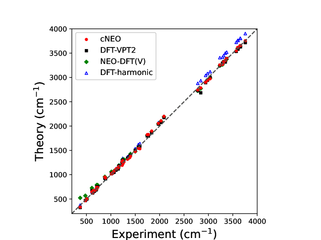
Figure 1: Experimental and theoretical vibrational frequencies for molecules in Table 2.

IV.3 Vibrational frequencies of proton transfer modes in systems with a shared proton

Proton transfer through hydrogen bonds is crucial for understanding dynamic properties in many chemical and biological systems. The nuclear quantum effect is believed to play an important role during the proton transfer process.(Tuckerman et al., 1997; Marx et al., 1999) Here we apply cNEO-DFT Hessian to 4 simple systems with shared protons, including FHF-, H3O2-, H5O2+ and N2H7+.

From geometry optimization, both DFT and cNEO-DFT predict the shared proton for FHF- and H5O2+ to be in the middle of the two heavy atoms. As for H3O2- and N2H7+, DFT gives a double-well potential energy surface and predicts the proton to be either on the left or on the right, whereas cNEO-DFT still predicts the proton to be in the middle. This is consistent with the results from previous literature and the reason is that when the proton is treated quantum mechanically, the vibrational zero-point energy washes out the low proton transfer barrier.(Asmis et al., 2007; Yang et al., 2008; Kaledin et al., 2009)

The experimental and computational vibrational frequencies for the proton transfer modes are presented in Table 3. Full-quantum cNEO-DFT overestimates the frequencies of FHF-, H3O2- and H5O2+ by 50-300 cm^-1 and accurately predict that of N2H7+. In contrast, DFT harmonic calculations severely overestimate the frequency of N2H7+ but seem to give acceptable results for the first three molecules. However, the bad performance of DFT-VPT2 and the large discrepancy between DFT and DFT-VPT2 show the failure of the perturbative treatment for these low-frequency modes and indicate that the DFT potential energy surfaces are not really reliable in these systems. In addition, the vibrational frequencies for these modes by DFT-VPT2 can be very sensitive to the choice of electronic exchange-correlation functionals. We compare the results by B3LYP and PBE0 in Table 3. A huge difference can be found for the anharmonic frequencies of the proton transfer mode of H3O2- and N2H7+ by DFT-VPT2. In contrast, cNEO-DFT is less sensitive to functional choice with B3LYP and PBE0 functionals giving similar results within 150 cm^-1. Previously anharmonic frequencies by VPT2 have also been found to be very sensitive to the choice of underlying computational methods and basis sets.(Hanson-Heine et al., 2012; Jacobsen et al., 2013) For example, for FHF-, VPT2 based on the coupled-cluster theory can give a much more accurate result (1313 cm^-1) than DFT-VPT2,(Hirata et al., 2008) and for N2H7+, MP2-VPT2 predicts a frequency of 485 cm^-1,(Wang and Agmon, 2016) which is also much closer to the experimental value than DFT-VPT2. Therefore, although VPT2 can give improved results with a more accurate underlying theory, cNEO-DFT is able to give reasonably good results based on commonly used density functionals with a much lower computational cost. This makes cNEO-DFT a promising method for the quantum description of protons in large chemical systems in future studies.

Table 3: Vibrational frequencies of FHF-, H3O2-, H5O2+ and N2H7+ (in cm^-1)

Molecule	Ptoton transfer mode	Experiment	Full-quantum cNEO-DFT			DFT-harmonic			DFT-VPT2
			B3LYP	PBE0		B3LYP	PBE0		B3LYP	PBE0
FHF-	F-H stretch	1331.2a	1584.5	1679.1		1286.3	1365.7		1550.1	1574.8
H3O2-	O-H stretch	697b	756.8	941.7		316.3	299.7		144.7i	1270.6i
H5O2+	O-H stretch	1085c	1181.0	1254.7		925.3	982.7		1406.6	1390.4
N2H7+	N-H stretch	374d	324.0	405.3		1727.9	1731.1		182.2	37.4

a. From Ref. 46

b. From Ref. 47

c. From Ref. 48

d. From Ref. 40

V Conclusion

In this work, we derived and implemented the first-order CPKS equation and the analytic Hessian for cNEO-DFT. The cNEO-CPKS equation incorporates the constraints on the nuclear expectation positions and solves the responses of electronic and nuclear orbitals to the changes of quantum nuclear expectation positions as well as classical nuclear positions. These responses are used in the calculation of cNEO-DFT analytic Hessian. Except diatomic molecules, cNEO-DFT are comparable to DFT-VPT2 in the description of molecular vibrational frequencies in polyatomic molecules. The incorporation of nuclear quantum effects in the energy surface enables cNEO-DFT to well describe many vibrational modes that were previously considered anharmonic with a simple harmonic treatment. These modes include the stretch and bend modes of X-H bonds, which are important in describing many chemical reactions. Compared to NEO-DFT(V), cNEO-DFT is also much more accurate and more efficient. For systems with shared protons, cNEO-DFT can be a more reliable method than DFT-VPT2 because the energy surface by cNEO-DFT includes nuclear quantum effects and is more reliable than the DFT potential energy surface for these challenging systems. These results indicate the good quality of the cNEO-DFT energy surface, and since Hessian can be used to characterize local minima and saddle points, this work makes cNEO-DFT a promising and viable method to include nuclear quantum effects in the study of chemical reactions through transition-state theory or molecular dynamics simulations in the future.

Supplementary Material

See the supplementary material for detailed derivation for the analytic Hessian of cNEO-DFT and a comparison of analytic and finite-difference results for molecular vibrational frequencies.

data avalibility

The data that support the findings of this study are available within the article and its supplementary material.

References

- Kreibich and Gross (2001) T. Kreibich and E. K. U. Gross, Phys. Rev. Lett. 86, 2984 (2001).
- Bochevarov et al. (2004) A. D. Bochevarov, E. F. Valeev, and C. D. Sherrill, Mol. Phys. 102, 111 (2004).
- Nakai (2007) H. Nakai, Int. J. Quantum Chem. 107, 2849 (2007).
- Ishimoto et al. (2009) T. Ishimoto, M. Tachikawa, and U. Nagashima, Int. J. Quantum Chem. 109, 2677 (2009).
- Abedi et al. (2010) A. Abedi, N. T. Maitra, and E. K. U. Gross, Phys. Rev. Lett. 105, 123002 (2010).
- Pavošević et al. (2020) F. Pavošević, T. Culpitt, and S. Hammes-Schiffer, Chem. Rev. 120, 4222 (2020).
- Ceriotti et al. (2016) M. Ceriotti, W. Fang, P. G. Kusalik, R. H. McKenzie, A. Michaelides, M. A. Morales, and T. E. Markland, Chem. Rev. 116, 7529 (2016).
- Guo et al. (2017) J. Guo, X.-Z. Li, J. Peng, E.-G. Wang, and Y. Jiang, Prog Surf Sci 92, 203 (2017).
- Webb et al. (2002) S. P. Webb, T. Iordanov, and S. Hammes-Schiffer, J. Chem. Phys. 117, 4106 (2002).
- Iordanov and Hammes-Schiffer (2003) T. Iordanov and S. Hammes-Schiffer, J. Chem. Phys. 118, 9489 (2003).
- Yang et al. (2018) Y. Yang, T. Culpitt, and S. Hammes-Schiffer, J. Phys. Chem. Lett. 9, 1765 (2018).
- Yang et al. (2019) Y. Yang, P. E. Schneider, T. Culpitt, F. Pavošević, and S. Hammes-Schiffer, J. Phys. Chem. Lett. 10, 1167 (2019).
- Schneider et al. (2021) P. E. Schneider, Z. Tao, F. Pavošević, E. Epifanovsky, X. Feng, and S. Hammes-Schiffer, J. Chem. Phys. 154, 054108 (2021).
- Xu and Yang (2020a) X. Xu and Y. Yang, J. Chem. Phys. 153, 074106 (2020a).
- Xu and Yang (2020b) X. Xu and Y. Yang, J. Chem. Phys. 152, 084107 (2020b).
- Pulay (2014) P. Pulay, WIREs Comput. Mol. Sci. 4, 169 (2014).
- Pople et al. (1979) J. A. Pople, R. Krishnan, H. B. Schlegel, and J. S. Binkley, Int. J. Quantum Chem. 16, 225 (1979).
- Pulay (1983) P. Pulay, J. Chem. Phys. 78, 5043 (1983).
- Komornicki and Fitzgerald (1993) A. Komornicki and G. Fitzgerald, J. Chem. Phys. 98, 1398 (1993).
- Yamaguchi and Schaefer III (2011) Y. Yamaguchi and H. F. Schaefer III, “Analytic derivative methods in molecular electronic structure theory: A new dimension to quantum chemistry and its applications to spectroscopy,” in Handbook of High-resolution Spectroscopy (2011) pp. 325–362.
- Sun et al. (2018) Q. Sun, T. C. Berkelbach, N. S. Blunt, G. H. Booth, S. Guo, Z. Li, J. Liu, J. D. McClain, E. R. Sayfutyarova, S. Sharma, S. Wouters, and G. K.-L. Chan, WIREs Comput Mol Sci 8, e1340 (2018).
- Sun et al. (2020) Q. Sun, X. Zhang, S. Banerjee, P. Bao, M. Barbry, N. S. Blunt, N. A. Bogdanov, G. H. Booth, J. Chen, Z.-H. Cui, J. J. Eriksen, Y. Gao, S. Guo, J. Hermann, M. R. Hermes, K. Koh, P. Koval, S. Lehtola, Z. Li, J. Liu, N. Mardirossian, J. D. McClain, M. Motta, B. Mussard, H. Q. Pham, A. Pulkin, W. Purwanto, P. J. Robinson, E. Ronca, E. R. Sayfutyarova, M. Scheurer, H. F. Schurkus, J. E. T. Smith, C. Sun, S.-N. Sun, S. Upadhyay, L. K. Wagner, X. Wang, A. White, J. D. Whitfield, M. J. Williamson, S. Wouters, J. Yang, J. M. Yu, T. Zhu, T. C. Berkelbach, S. Sharma, A. Y. Sokolov, and G. K.-L. Chan, J. Chem. Phys. 153, 024109 (2020).
- Becke (1988) A. D. Becke, Phys. Rev. A 38, 3098 (1988).
- Lee et al. (1988) C. Lee, W. Yang, and R. G. Parr, Phys. Rev. B 37, 785 (1988).
- Becke (1993) A. D. Becke, J. Chem. Phys. 98, 5648 (1993).
- Scott and Radom (1996) A. P. Scott and L. Radom, J. Phys. Chem. 100, 16502 (1996).
- Dunning (1989) T. H. Dunning, J. Chem. Phys. 90, 1007 (1989).
- Bardo and Ruedenberg (1974) R. D. Bardo and K. Ruedenberg, J. Chem. Phys. 60, 918 (1974).
- Larsen et al. (2017) A. H. Larsen, J. J. Mortensen, J. Blomqvist, I. E. Castelli, R. Christensen, M. Du\lak, J. Friis, M. N. Groves, B. Hammer, C. Hargus, E. D. Hermes, P. C. Jennings, P. B. Jensen, J. Kermode, J. R. Kitchin, E. L. Kolsbjerg, J. Kubal, K. Kaasbjerg, S. Lysgaard, J. B. Maronsson, T. Maxson, T. Olsen, L. Pastewka, A. Peterson, C. Rostgaard, J. Schiøtz, O. Schütt, M. Strange, K. S. Thygesen, T. Vegge, L. Vilhelmsen, M. Walter, Z. Zeng, and K. W. Jacobsen, J. Phys.: Condens. Matter 29, 273002 (2017).
- Barone (2005) V. Barone, J. Chem. Phys. 122, 014108 (2005).
- Frisch et al. (2016) M. J. Frisch, G. W. Trucks, H. B. Schlegel, G. E. Scuseria, M. A. Robb, J. R. Cheeseman, G. Scalmani, V. Barone, G. A. Petersson, H. Nakatsuji, X. Li, M. Caricato, A. V. Marenich, J. Bloino, B. G. Janesko, R. Gomperts, B. Mennucci, H. P. Hratchian, J. V. Ortiz, A. F. Izmaylov, J. L. Sonnenberg, D. Williams-Young, F. Ding, F. Lipparini, F. Egidi, J. Goings, B. Peng, A. Petrone, T. Henderson, D. Ranasinghe, V. G. Zakrzewski, J. Gao, N. Rega, G. Zheng, W. Liang, M. Hada, M. Ehara, K. Toyota, R. Fukuda, J. Hasegawa, M. Ishida, T. Nakajima, Y. Honda, O. Kitao, H. Nakai, T. Vreven, K. Throssell, J. A. Montgomery, Jr., J. E. Peralta, F. Ogliaro, M. J. Bearpark, J. J. Heyd, E. N. Brothers, K. N. Kudin, V. N. Staroverov, T. A. Keith, R. Kobayashi, J. Normand, K. Raghavachari, A. P. Rendell, J. C. Burant, S. S. Iyengar, J. Tomasi, M. Cossi, J. M. Millam, M. Klene, C. Adamo, R. Cammi, J. W. Ochterski, R. L. Martin, K. Morokuma, O. Farkas, J. B. Foresman, and D. J. Fox, “Gaussian 16 Revision C.01,” (2016), gaussian Inc. Wallingford CT.
- Culpitt et al. (2019a) T. Culpitt, Y. Yang, P. E. Schneider, F. Pavošević, and S. Hammes-Schiffer, J. Chem. Theory Comput. 15, 6840 (2019a).
- Culpitt et al. (2019b) T. Culpitt, Y. Yang, F. Pavošević, Z. Tao, and S. Hammes-Schiffer, J. Chem. Phys. 150, 201101 (2019b).
- Habershon et al. (2008) S. Habershon, G. S. Fanourgakis, and D. E. Manolopoulos, J. Chem. Phys. 129, 074501 (2008).
- Kaczmarek et al. (2009) A. Kaczmarek, M. Shiga, and D. Marx, J. Phys. Chem. A 113, 1985 (2009).
- Calvo et al. (2014) F. Calvo, C. Falvo, and P. Parneix, J. Phys. Chem. A 118, 5427 (2014).
- Tuckerman et al. (1997) M. E. Tuckerman, D. Marx, M. L. Klein, and M. Parrinello, Science 275, 817 (1997).
- Marx et al. (1999) D. Marx, M. E. Tuckerman, J. Hutter, and M. Parrinello, Nature 397, 601 (1999).
- Asmis et al. (2007) K. R. Asmis, Y. Yang, G. Santambrogio, M. Brümmer, J. R. Roscioli, L. R. McCunn, M. A. Johnson, and O. Kühn, Angew. Chem. - Int. Ed. 46, 8691 (2007).
- Yang et al. (2008) Y. Yang, O. Kühn, G. Santambrogio, D. J. Goebbert, and K. R. Asmis, J. Chem. Phys. 129, 224302 (2008).
- Kaledin et al. (2009) M. Kaledin, J. M. Moffitt, C. R. Clark, and F. Rizvi, J. Chem. Theory Comput. 5, 1328 (2009).
- Hanson-Heine et al. (2012) M. W. D. Hanson-Heine, M. W. George, and N. A. Besley, J. Phys. Chem. A 116, 4417 (2012).
- Jacobsen et al. (2013) R. L. Jacobsen, R. D. Johnson, K. K. Irikura, and R. N. Kacker, J. Chem. Theory Comput. 9, 951 (2013).
- Hirata et al. (2008) S. Hirata, K. Yagi, S. Ajith Perera, S. Yamazaki, and K. Hirao, J. Chem. Phys. 128, 214305 (2008).
- Wang and Agmon (2016) H. Wang and N. Agmon, J. Phys. Chem. A 120, 3117 (2016).
- Kawaguchi and Hirota (1987) K. Kawaguchi and E. Hirota, J. Chem. Phys. 87, 6838 (1987).
- Diken et al. (2005) E. G. Diken, J. M. Headrick, J. R. Roscioli, J. C. Bopp, M. A. Johnson, and A. B. McCoy, J. Phys. Chem. A 109, 1487 (2005).
- Headrick (2005) J. M. Headrick, Science 308, 1765 (2005).