The effects of degree distributions in random networks of Type-I neurons

Abstract

We consider large networks of theta neurons and use the Ott/Antonsen ansatz to derive degree-based mean field equations governing the expected dynamics of the networks. Assuming random connectivity we investigate the effects of varying the widths of the in- and out-degree distributions on the dynamics of excitatory or inhibitory synaptically coupled networks, and gap junction coupled networks. For synaptically coupled networks, the dynamics are independent of the out-degree distribution. Broadening the in-degree distribution destroys oscillations in inhibitory networks and decreases the range of bistability in excitatory networks. For gap junction coupled neurons, broadening the degree distribution varies the values of parameters at which there is an onset of collective oscillations. Many of the results are shown to also occur in networks of more realistic neurons.

I Introduction

It is well-known that the structure of a network can have a significant effect on its dynamics. One type of network of great interest is that of networks of neurons, and much effort has gone into investigating this issue rox11 ; schkih15 ; nykfri17 ; marhou16 ; perdeg13 . In networks of neurons, the nodes are normally thought of an individual neurons, while the edges describe connections between neurons. These connections can be directed (in the case of synaptic connections ermter10 ) or undirected (in the case of gap junction connections Benzuk04 ; erm06 ). One of the important properties of a node in a network is its degree: a node’s in-degree is the number of connections to it, and a node’s out-degree is the number of connections from it. In the case of undirected connections a node simply has a degree, as there is no distinction between incoming or outgoing connections. Previous work on understanding the dynamics of networks of neurons has considered the effects of correlations between the in- and out-degrees of individual neurons laibla20 ; lamsmi10 ; marhou16 ; vashou12 ; vegrox19 ; nykfri17 and of degree assortativity, in which the probability that two neurons are connected is influenced by the degrees of the two neurons blasche2020 ; kahsok17 ; schkih15 ; defranciscis2011 .

In this paper we consider the effects of varying the widths of the distributions of in-degrees and out-degrees on large, randomly connected networks of Type-I neurons, i.e., neurons whose onset of firing is through a saddle-node-on-invariant-circle (SNIC) bifurcation. The analysis is done of networks of theta neurons, as these are the normal form of the SNIC bifurcation. They also have the property of being amenable to the use of the Ott/Antonsen ansatz ottant08 ; ottant09 , a now well-used method for deriving equations governing the evolution of order parameter-like quantities, valid for large networks with particular forms of heterogeneity lai14A ; lai09A ; lukbar13 ; resott14 ; chahat17 .

A common assumption in creating random networks of neurons is that there is a fixed probability of connecting any two neurons tatolm12 ; golde10 . Such networks are often referred to as Erdös-Rényi and have a binomial distribution of degrees, with the ratio of mean degree to standard deviation of degrees going to zero as network size goes to infinity. However, real networks of neurons are observed to have properties incompatible with this assumption sonsjo05 .

Previous work on investigating the effects of degree distributions includes that of Roxin rox11 . He found in an inhibitory network of leaky integrate-and-fire neurons that broadening the distribution of in-degrees suppressed macroscopic oscillations. This result was reproduced in a simplified rate model which included the heterogeneity in neuronal input due to the in-degree of cells. He also considered a network with both excitatory and inhibitory neurons and investigated the effects of varying the in- and out-degree distributions of the recurrent excitatory connections. In other work, qinche18 studied the effects of degree distribution in feedforward networks.

We consider synaptic coupling in Sec. II and gap junction coupling in Sec. III. Both sections start with a derivation of the relevant equations using the Ott/Antonsen ansatz and then give some numerical results. Most results use Lorentzian distributions of heterogeneous parameters, and in Sec. IV we briefly discuss results using normal and uniform distributions. We conclude in Sec. V. Appendix A contains the description of the network of Morris-Lecar neurons used to verify some of the results derived for networks of theta neurons.

II Synaptic coupling

We first consider networks of theta neurons coupled by synaptic input currents with a timescale $\tau$. Alternative formulations could model synaptic input by using dynamic synapses coobyr19 or input current pulses with both a rise time and a decay time ermter10 .

II.1 Model and Theory

We consider a network of $N$ theta neurons, each of which has dynamics described by

$$\frac{d\theta_{i}}{dt}=1-\cos{\theta_{i}}+(1+\cos{\theta_{i}})(\eta_{i}+I_{i}(t))$$ (1)

for $i=1,\dots N$, where the input current to neuron $i$ is

$$I_{i}(t)=\frac{K}{\langle k\rangle}\sum_{j=1}^{N}A_{ij}u_{j}(t)$$ (2)

and the synaptic variables have dynamics given by

$$\tau\frac{du_{j}}{dt}=\sum_{m\in\mathbb{Z}}\delta(t-T_{j}^{m})-u_{j},$$ (3)

where $T_{j}^{m}$ is the $m$th firing time of neuron $j$, defined to happen every time $\theta_{j}$ increases through $\pi$, and $\delta(\cdot)$ is the Dirac delta. Thus every time $\theta_{j}$ increases through $\pi$, $u_{j}$ is instantaneously incremented by an amount $1/\tau$, and between firing times it decays as $\sim e^{-t/\tau}$. $K$ is the strength of connections between neurons (which may be positive or negative), $\langle k\rangle$ is the average in-degree in the network, and $A$ describes the connectivity of the network, i.e., $A_{ij}=1$ if there is a connection from neuron $j$ to neuron $i$ and $A_{ij}=0$ otherwise. We have $\langle k\rangle=\sum_{i,j}A_{i,j}/N$. The $\eta_{i}$ are randomly chosen from a Lorentzian

$$g(\eta)=\frac{\Delta/\pi}{(\eta-\eta_{0})^{2}+\Delta^{2}}$$ (4)

with centre $\eta_{0}$ and half-width-at-half-maximum (HWHM) $\Delta$, which introduces heterogeneity to the network. The Lorentzian is chosen so that analytical progress can be made. We discuss results for other distributions below.

If the input current $I_{i}$ is constant, the theta neuron shows one of two types of behaviour. For $\eta_{i}+I_{i}<0$, (1) has two fixed points, one stable and one unstable. For $\eta_{i}+I_{i}>0$, (1) has no fixed points and $\theta_{i}$ increases with time, showing periodic oscillations with frequency $\sqrt{\eta_{i}+I_{i}}/\pi$ erm96 . The bifurcation at $\eta_{i}+I_{i}=0$ is a SNIC bifurcation. Note that under the transformation $V=\tan{(\theta/2)}$ a network of theta neurons is exactly equivalent to a network of quadratic integrate-and-fire neurons with infinite threshold and reset values bor17 . We now proceed to analyse the network dynamics, using ideas similar to those in chahat17 ; blasche2020 ; laibla20 ; resott14 ; laibla21 .

We assume that the network is characterised by two functions: firstly the degree distribution $P({\bf k})$, normalised to sum to 1, where ${\bf k}=(k_{in},k_{out})$ and $k_{in}$ and $k_{out}$ are the in- and out-degrees of a neuron with degree ${\bf k}$, respectively, and secondly the assortativity function $a({\bf k}^{\prime}\to{\bf k})$ giving the probability of a connection from a neuron with degree ${\bf k}^{\prime}$ to one with degree ${\bf k}$, given that such neurons exist. We also make the mean field assumption that the dynamics of a neuron depend only on its degree ${\bf k}$, thus effectively averaging the dynamics of all neurons with the same degree.

In the limit of large $N$ and large in- and out-degrees, the network is described by the distribution $f(\theta,\eta|{\bf k},t)$ where $f(\theta,\eta|{\bf k},t)d\theta d\eta$ is the probability that a neuron with degree ${\bf k}$ has phase in $[\theta,\theta+d\theta]$ and value of $\eta$ in $[\eta,\eta+d\eta]$ at time $t$. This distribution satisfies the continuity equation

$$\frac{\partial f}{\partial t}+\frac{\partial}{\partial\theta}(vf)=0$$ (5)

where (from (1)-(3))

$$v(\theta,{\bf k},\eta,t)=1-\cos{\theta}+(1+\cos{\theta})[\eta+I({\bf k},t)],$$ (6)

$$I({\bf k},t)=\frac{KN}{\langle k\rangle}\sum_{{\bf k}^{\prime}}P({\bf k}^{\prime})a({\bf k}^{\prime}\to{\bf k})u({\bf k}^{\prime},t),$$ (7)

and

$$\tau\frac{du({\bf k},t)}{dt}=\widehat{F}({\bf k},t)-u({\bf k},t),$$ (8)

where $\widehat{F}({\bf k},t)$ is the firing rate of neurons with degree ${\bf k}$ at time $t$.

The Ott/Antonsen ansatz gives the dynamics for the order parameter for neurons with degree ${\bf k}$ laibla20 ; blasche2020 ; lai14A :

$$\frac{\partial b({\bf k},t)}{\partial t}=\frac{-i[b({\bf k},t)-1]^{2}}{2}+\frac{[b({\bf k},t)+1]^{2}}{2}$$

$$\times\left[-\Delta+i\eta_{0}+i\frac{KN}{\langle k\rangle}\sum_{{\bf k}^{\prime}}P({\bf k}^{\prime})a({\bf k}^{\prime}\to{\bf k})u({\bf k}^{\prime},t)\right]$$

where $b({\bf k},t)$ is the expected value of $e^{i\theta}$ for neurons with degree ${\bf k}$, i.e.

$$b({\bf k},t)=\int_{-\infty}^{\infty}\int_{0}^{2\pi}f(\theta,\eta|{\bf k},t)e^{i\theta}d\theta\ d\eta.$$ (9)

The firing rate of neurons with degree ${\bf k}$ at time $t$ is the expected value of the flux through $\theta=\pi$ lai15 ; monpaz15 , i.e.

$$\widehat{F}({\bf k},t)=\int_{-\infty}^{\infty}f(\pi,\eta|{\bf k},t)d\eta=\frac{1}{\pi}\mbox{Re}\left(\frac{1-\bar{b}({\bf k},t)}{1+\bar{b}({\bf k},t)}\right)$$ (10)

where the overline indicates conplex conjugate. We define $F(b({\bf k},t))\equiv\widehat{F}({\bf k},t)$.

With neutral assortativity resott14 ,

$$a({\bf k}^{\prime}\to{\bf k})=\frac{k_{out}^{\prime}k_{in}}{N\langle k\rangle}$$ (11)

and with independent in- and out-degrees the degree distribution $P({\bf k}^{\prime})$ factorises as $P({\bf k}^{\prime})=p_{in}(k_{in}^{\prime})p_{out}(k_{out}^{\prime})$, where $p_{in}$ and $p_{out}$ are the marginal distributions of the relevant degrees, so

$$\frac{KN}{\langle k\rangle}\sum_{{\bf k}^{\prime}}P({\bf k}^{\prime})a({\bf k}^{\prime}\to{\bf k})u({\bf k}^{\prime},t)$$ (12)

$$=\frac{Kk_{in}}{\langle k\rangle^{2}}\sum_{k_{in}^{\prime}}\sum_{k_{out}^{\prime}}p_{in}(k_{in}^{\prime})p_{out}(k_{out}^{\prime})k_{out}^{\prime}u(k_{in}^{\prime},k_{out}^{\prime},t).$$

This quantity is independent of $k_{out}$ and contributes to the “input” to neurons with degree ${\bf k}$. Thus $b({\bf k},t)$ must also be independent of $k_{out}$ and so must $F(b({\bf k},t))$ and $u({\bf k},t)$. Thus (12) simplifies to

$$\frac{KN}{\langle k\rangle}\sum_{{\bf k}^{\prime}}P({\bf k}^{\prime})a({\bf k}^{\prime}\to{\bf k})u({\bf k}^{\prime},t)$$

$$=\frac{Kk_{in}}{\langle k\rangle}\sum_{k_{in}^{\prime}}p_{in}(k_{in}^{\prime})u(k_{in}^{\prime},t)$$ (13)

and we see that the distribution of out-degrees does not affect the expected dynamics. This was observed by Roxin in rox11 , although he observed that broadening the out-degree distribution increases the amplitude of the cross-correlation of synaptic currents, something we do not consider here.

We have

$$\tau\frac{du(k_{in},t)}{dt}=F(b(k_{in},t))-u(k_{in},t),$$ (14)

and defining

$$s(t)\equiv\sum_{k_{in}}p_{in}(k_{in})u(k_{in},t)$$ (15)

we see that $s$ satisfies

$$\tau\frac{ds}{dt}=\sum_{k_{in}}p_{in}(k_{in})F(b(k_{in},t))-s$$ (16)

and the dynamics of $b$ are given by

$$\frac{\partial b(k_{in},t)}{\partial t}=\frac{-i[b(k_{in},t)-1]^{2}}{2}$$

$$+\frac{[b(k_{in},t)+1]^{2}}{2}\left[-\Delta+i\eta_{0}+\frac{iKk_{in}s}{\langle k\rangle}\right].$$ (17)

Equations (16)-(17) form a set of $N_{k_{in}}+1$ ordinary differential equations (ODEs) governing the network’s dynamics, where $N_{k_{in}}$ is the number of distinct in-degrees in the network. In the next section we give some numerical results showing the possible dynamics of this set of equations.

II.2 Results

We first consider inhibitory coupling, i.e., $K<0$.

II.2.1 Inhibitory coupling

Consider the parameter values $\eta_{0}=1,\Delta=0.05,\tau=1,K=-2,\langle k\rangle=100$. Having $\eta_{0}>0$ indicates that when uncoupled, most neurons would be firing rather than quiescent. We choose $p_{in}$ to be uniform with mean $\langle k\rangle=100$ and write its support as $[100-\sigma,100+\sigma]$. For $\sigma=5$ (a narrow distribution) we obtain global oscillations, see Fig. 1(a). However, when the in-degree distribution is made broader ($\sigma=50$), the oscillations die out: see Fig. 1(b). Note the independence of the dynamics on the distribution of out-degrees, $p_{out}(k_{out})$, as expected.

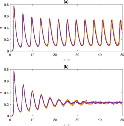
Figure 1: (a) $s$ for the reduced model (16)-(17) (blue curve) and for the full model (1)-(3) (dots) for $p_{out}$ being uniform on $[10,190],[50,150]$ and $[90,110]$ (different colours). $p_{in}$ is uniform on $[95,105]$ (i.e. $\sigma=5$). A different realisation of the $\eta_{i}$ was used for the different networks. (b): as for (a) but now $p_{in}$ is uniform on $[50,150]$ ($\sigma=50$). For  (1)-(3) $N=500$ neurons were used and the initial conditions were $\theta_{i}=u_{i}=0$, and for (16)-(17) we used $b=1$ and $s=0$.

To numerically solve (16)-(17) we treat $k_{in}$ as a continuous variable and discretise the support of $p_{in}$ using 100 evenly spaced points, and use $p_{in}=1/100$ at each of those points, effectively using the midpoint rule. To create the network used in (1)-(3) we randomly sample $N$ in-degrees from $p_{in}(k_{in})$ and $N$ out-degrees from $p_{out}(k_{out})$, choosing until the sum of the in-degrees equals the sum of the out-degrees, then use the configuration model to connect the network new03 . Any self or multiple connections are then removed by random rewiring, keeping the degrees fixed. To solve (1)-(3) we used Euler’s method with a stepsize of $0.001$.

The destruction of oscillations seen in Fig. 1 seems due to a Hopf bifurcation. Using pseudo-arclength continuation to follow the stable fixed point of (16)-(17) as $\sigma$ is decreased we find a Hopf bifurcation at $\sigma\approx 31.4$, and continuing that bifurcation as both $\sigma$ and $\tau$ are varied we obtain the curve in Fig. 2. For any $\tau$ for which an oscillation occurs, increasing $\sigma$ will destroy the oscillations, and for small $\sigma$, a value of $\tau$ which is either too large or too small will also destroy oscillations. (We varied $\tau$ here just as an example; we could equally well vary other parameters such as $\eta_{0}$ or $\Delta$.) The destruction of oscillations in an inhibitory network by broadening the in-degree distribution was also observed by Roxin rox11 . He analysed a heuristic rate model containing a fixed delay (since he used delayed synapses) and found a Hopf bifurcation in that model, in agreement with the results shown here.

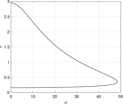
Figure 2: Hopf bifurcation curve for a fixed point of (16)-(17). A stable periodic orbit exists to the left of the curve and a stable fixed point to the right. Other parameters: $\eta_{0}=1,\Delta=0.05,K=-2,\langle k\rangle=100$. $p_{in}$ is uniform on $[100-\sigma,100+\sigma]$.

To investigate the generality of our result we now consider a beta distribution of in-degrees, with equal parameters greater than one, shifted to have mean 100 and support on $[50,150]$, i.e.

$$p_{in}(k_{in})=\begin{cases}Cx^{\alpha-1}(1-x)^{\alpha-1},&0\leq x\leq 1\\ 0,&\mbox{otherwise}\end{cases}$$ (18)

where $x=(k_{in}-50)/100$ and $C$ is a normalisation factor. Increasing $\alpha$ narrows the distribution, as shown in the inset of Fig. 3. Varying $\alpha$ and $\tau$ we find a curve of Hopf bifurcations, shown in Fig. 3, which shows the same qualitative behaviour as for the uniform distribution.

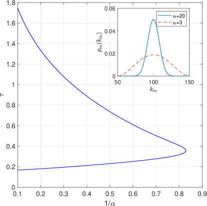
Figure 3: A beta distribution of in-degrees. Hopf bifurcation curve for fixed point of (16)-(17). A stable periodic orbit exists to the left of the curve and a stable fixed point to the right. Other parameters: $\eta_{0}=1,\Delta=0.05,K=-2,\langle k\rangle=100$. Inset shows the beta distribution on $[50,150]$ with $\alpha=3,20$.

To further demonstrate the generality of our results we now consider a network of 500 Morris-Lecar neurons tsukit06 , known to undergo a SNIC bifurcation as the input current is increased laibla20 . The network equations are given in Appendix A. The in-degree distribution is uniform on $[100-\sigma,100+\sigma]$ and the out-degree is uniform on $[50,150]$. For each different value of $\sigma$ we generate a network as explained above and for each network we vary $\tau$, the synaptic timescale, integrating for $50$ seconds at each value of $\tau$. Defining $\hat{s}=N^{-1}\sum_{i=1}^{N}s_{i}$ we discard data from the first $45$ seconds and calculate the standard deviation of $\hat{s}$ over the last 5 seconds, plotting that in Fig. 4. Large values indicate oscillations while small values indicate an approximate steady state. We see results consistent with those in Figs. 2 and 3. Thus we conclude that broadening the in-degree distribution of an inhibitory network of Type-I neurons acts to destroy global oscillatory behaviour. This is presumably due to having a wider range of dynamics for neurons with different in-degrees, making them harder to synchronise. We now consider excitatory coupling, i.e., $K>0$.

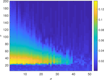
Figure 4: Results for a Morris-Lecar model. $\tau$ is the synaptic timescale and the in-degree distribution is uniform on $[100-\sigma,100+\sigma]$. Colour shows the standard deviation of $\hat{s}$ over 5 seconds of simulated time, having discarded the first 45 seconds. The same $\eta_{i}$ were used for each simulation. We used $N=500$ neurons.

II.2.2 Excitatory coupling

Consider the parameter values $\Delta=0.05,\tau=1,K=5,\langle k\rangle=100$. Varying $\eta_{0}$ we expect a region of bistability between a high activity steady state and a low activity steady state, as is often found in excitatory networks lailon03 . This is found, as shown in Fig. 5, where saddle-node bifurcations mark the boundaries of the bistable region. Varying the width of the in-degree distribution ($\sigma$) varies the width of the bistable region. In particular, widening the in-degree distribution narrows the width of the bistable region. Following the saddle-node bifurcations seen in Fig. 5 we obtain Fig. 6. Similar behaviour was seen for a beta distribution of in-degrees (not shown).

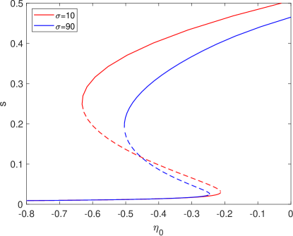
Figure 5: $s$ at fixed points of (16)-(17) for $\sigma=10$ (red) and $\sigma=90$ (blue). Solid curves are stable, dashed unstable. Parameters: $\Delta=0.05,\tau=1,K=5,\langle k\rangle=100$, uniform in-degree on $[100-\sigma,100+\sigma]$.

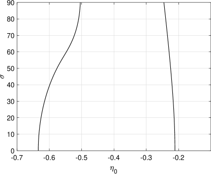
Figure 6: Curves of saddle-node bifurcations of fixed points of (16)-(17). The network is bistable between the curves and has a single attractor outside this region. Fig. 5 corresponds to horizontal “slices” through this figure at $\sigma=10$ and $\sigma=90$. Parameters: $\Delta=0.05,\tau=1,K=5,\langle k\rangle=100$, uniform in-degree on $[100-\sigma,100+\sigma]$.

We reproduced this behaviour in a network of $N=500$ Morris-Lecar neurons with parameters as given in Appendix A. For networks with $\sigma=10$ and $90$ we quasistatically varied $I_{0}$, integrating for $10$ seconds at each value. We define $\bar{s}$ to be the mean of $\hat{s}$ over the last $2$ seconds of simulation and plot this in Fig. 7. The results are qualitatively the same as in Fig. 5: $\bar{s}$ is lower when $\sigma=90$ than when $\sigma=10$, and the left-most saddle-node bifurcation is moved more than the right-most when $\sigma$ is varied. The threshold for firing for single neuron is $I_{0}\approx 39.69$ so the jumps occur at values of $I_{0}$ less than this, consistent with the results in Fig. 6. Thus we conclude that for an excitatory network of Type-I neurons, broadening the in-degree distribution narrows the range of values of the mean input for which the network is bistable. The effects of varying other parameters could equally well be investigated using the techniques shown here.

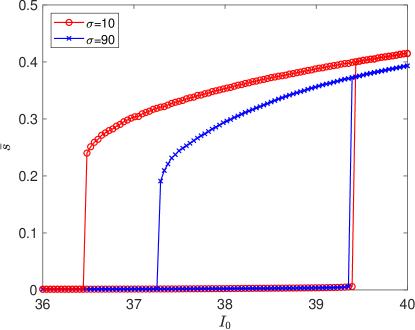
Figure 7: Approximate steady states for a Morris-Lecar model. For each of the two networks $I_{0}$ was quasistatically increased up and then down. Both networks show bistability for a range of $I_{0}$ values, and vertical jumps at apparent saddle-node bifurcations. Compare with Fig. 5. Parameters: $\langle k\rangle=100$, uniform in-degree on $[100-\sigma,100+\sigma]$, out-degree is uniform on $[50,150]$. The same $\eta_{i}$ were used for each simulation.

III Gap junctions

We now consider theta neurons coupled by gap junctions Benzuk04 ; galhes99 . Gap junctional coupling is well-known to induce synchrony in networks of neuronsostbru09 ; erm06 ; trakop01 . The quadratic integrate-and-fire (QIF) neuron latric00 with infinite firing threshold and reset to $V=-\infty$ is equivalent under the transformation $V=\tan{(\theta/2)}$ to a theta neuron ermkop86 , and since gap junction coupling is through voltage differences it is easier to start with a network of QIF neurons. Our analysis is similar to that in lai15 ; also see monpaz20 ; piedev19 ; Byrros20 . A theta neuron is an excitable system, so our results add to those on coupled excitable systems lafcol10 ; shikur86 ; chistr08 ; zhepik19 .

III.1 Model and Theory

Consider a network of $N$ gap-junction coupled QIF neurons governed by

$$\frac{dV_{j}}{dt}=\eta_{j}+V_{j}^{2}+\frac{g}{\langle k\rangle}\sum_{l=1}^{N}A_{jl}(V_{l}-V_{j})$$ (19)

for $j=1,\dots N$ together with the rule that if $V_{j}(t^{-})=\infty$ then $V_{j}(t^{+})=-\infty$, and neuron $j$ is said to fire at this time $t$. $A$ describes the connectivity of the network, where $A_{jl}=1$ if neurons $j$ and $l$ are connected and zero otherwise. Since gap junctional coupling is not directional we have $A_{jl}=A_{lj}$. $k_{j}$ is the degree of the $j$th neuron, i.e. $k_{j}=\sum_{l}A_{jl}$, $\langle k\rangle$ is the mean degree, as above, and $g$ is the strength of coupling (non-negative). The $\eta_{j}$ are randomly chosen from a distribution $h(\eta)$.

We rewrite (19) as

$$\frac{dV_{j}}{dt}=\eta_{j}+V_{j}^{2}-\frac{gk_{j}V_{j}}{\langle k\rangle}+\frac{g}{\langle k\rangle}\sum_{l=1}^{N}A_{jl}V_{l}.$$ (20)

Now let $V_{j}=\tan{(\theta_{j}/2)}$. Then

$$\frac{dV_{j}}{dt} =\frac{d\theta_{j}/dt}{2\cos^{2}{(\theta_{j}/2)}}$$

$$=\eta_{j}+\tan^{2}{(\theta_{j}/2)}-\frac{gk_{j}}{\langle k\rangle}\tan{(\theta_{j}/2)}$$

$$+\frac{g}{\langle k\rangle}\sum_{l=1}^{N}A_{jl}\tan{(\theta_{l}/2)}$$ (21)

so

$$\frac{d\theta_{j}}{dt}=1-\cos{\theta_{j}}+(1+\cos{\theta_{j}})$$

$$\times\left[\eta_{j}-\frac{gk_{j}}{\langle k\rangle}\tan{(\theta_{j}/2)}+\frac{g}{\langle k\rangle}\sum_{l=1}^{N}A_{jl}\tan{(\theta_{l}/2)}\right].$$ (22)

Noting that

$$\tan{(\theta/2)}=\frac{\sin{\theta}}{1+\cos{\theta}},$$ (23)

we have

$$\frac{d\theta_{j}}{dt}=1-\cos{\theta_{j}}-\frac{gk_{j}}{\langle k\rangle}\sin{\theta_{j}}+(1+\cos{\theta_{j}})$$

$$\times\left[\eta_{j}+\frac{g}{\langle k\rangle}\sum_{l=1}^{N}A_{jl}\tan{(\theta_{l}/2)}\right].$$ (24)

When a neuron fires, at $\theta=\pi$, the term involving $\tan$ becomes infinite. To avoid this problem we follow erm06 and replace $\tan{(\theta/2)}$ in (24) by

$$q(\theta)\equiv\frac{\sin{\theta}}{1+\cos{\theta}+\epsilon},$$ (25)

where $0<\epsilon\ll 1$, thereby removing the singularity. We take the limit $\epsilon\to 0$ below.

We analyse the system in a similar way as in Sec. II. The system is described by the probability density function $f(\eta,\theta|{\bf k},t)$ which satisfies ome14 ; str00 ; abrmir08

$$\frac{\partial f}{\partial t}+\frac{\partial}{\partial\theta}(fv)=0,$$ (26)

where

$$v(\eta,\theta,{\bf k},t)\equiv 1-\cos{\theta}-\frac{gk_{in}}{\langle k\rangle}\sin{\theta}$$

$$+(1+\cos{\theta})\left[\eta+gT({\bf k},t)\right],$$ (27)

where

$$T({\bf k},t)\equiv\frac{N}{\langle k\rangle}\sum_{{\bf k}^{\prime}}P({\bf k}^{\prime})a({\bf k}^{\prime}\rightarrow{\bf k})Q({\bf k}^{\prime},t),$$ (28)

$$Q({\bf k}^{\prime},t)=\int_{-\infty}^{\infty}\int_{0}^{2\pi}f(\eta,\theta|{\bf k}^{\prime},t)q(\theta)\ d\theta\ d\eta$$ (29)

and ${\bf k}=(k_{in},k_{out})$, $P({\bf k}^{\prime})$ is the distribution of degrees of a neuron, and $a({\bf k}^{\prime}\rightarrow{\bf k})$ is the probability of a connection from a neuron with degree ${\bf k}^{\prime}$ to one with degree ${\bf k}$. But connections are undirected, so a neuron just has a degree. Thus we write

$$T(k,t)=\frac{N}{\langle k\rangle}\sum_{k^{\prime}}P(k^{\prime})a(k^{\prime}\rightarrow k)Q(k^{\prime},t)$$ (30)

where $P(k)$ is the degree distribution, and

$$Q(k^{\prime},t)=\int_{-\infty}^{\infty}\int_{0}^{2\pi}f(\eta,\theta|k^{\prime},t)q(\theta)\ d\theta\ d\eta$$ (31)

is the expected value of $q(\theta)$ for neurons with degree $k^{\prime}$ at time $t$. From lai15 , assuming that $h(\eta)$ is a Lorentzian with median $\eta_{0}$ and HWHM $\Delta$, we have

$$\frac{\partial b(k,t)}{\partial t}=\frac{(i\eta_{0}-\Delta)(1+b)^{2}-i(1-b)^{2}}{2}$$

$$+\frac{i(1+b)^{2}gT+g(1-b^{2})}{2}$$ (32)

where $T(k,t)$ and $Q(k^{\prime},t)$ are as above and

$$b(k,t)=\int_{-\infty}^{\infty}\int_{0}^{2\pi}f(\eta,\theta|k,t)e^{i\theta}\ d\theta\ d\eta$$ (33)

is the complex-valued order parameter for neurons with degree $k$ at time $t$.

By expanding $q(\theta)$ in a Fourier series it was shown in lai15 that

$$Q(k^{\prime},t)=\sum_{m=1}^{\infty}\left[c_{m}b(k^{\prime},t)^{m}+\mbox{c.c.}\right]$$ (34)

where “c.c.” is the complex conjugate of the previous term and

$$c_{m}=\frac{i[(\sqrt{2\epsilon+\epsilon^{2}}-1-\epsilon)^{m+1}-(\sqrt{2\epsilon+\epsilon^{2}}-1-\epsilon)^{m-1}]}{2\sqrt{2\epsilon+\epsilon^{2}}}.$$ (35)

Recently, piedev19 showed that

$$\lim_{\epsilon\rightarrow 0}c_{m}=i(-1)^{m}$$ (36)

and thus

$$Q(k^{\prime},t)=i\sum_{m=1}^{\infty}(-1)^{m}[b(k^{\prime},t)^{m}-\bar{b}(k^{\prime},t)^{m}]$$

$$=\frac{2\mbox{Im}[b(k^{\prime},t)]}{[1+b(k^{\prime},t)][1+\bar{b}(k^{\prime},t)]}$$ (37)

where we have summed the geometric series.

Defining

$$w\equiv\frac{1-\bar{b}}{1+\bar{b}}$$ (38)

(so $b=(1-\bar{w})/(1+\bar{w})$) we find that $w$ satisfies

$$\frac{\partial w(k,t)}{\partial t}=i\eta_{0}+\Delta-i[w(k,t)]^{2}+igT(k,t)-gw(k,t),$$ (39)

and writing $w=\pi\phi+iV$ where $\phi$ and $V$ are real we find that $Q(k^{\prime},t)=V(k^{\prime},t)$ and the real and imaginary parts of (39) give

$$\frac{\partial\phi(k,t)}{dt} =\frac{\Delta}{\pi}+2\phi(k,t)V(k,t)-g\phi(k,t)$$ (40)

$$\frac{\partial V(k,t)}{dt} =\eta_{0}-\pi^{2}[\phi(k,t)]^{2}+[V(k,t)]^{2}$$

$$+g[T(k,t)-V(k,t)]$$ (41)

where

$$T(k,t)=\frac{N}{\langle k\rangle}\sum_{k^{\prime}}P(k^{\prime})a(k^{\prime}\rightarrow k)V(k^{\prime},t).$$ (42)

The interpretation of $\phi$ and $V$ is that $\phi(k,t)$ is the expected firing frequency of neurons with degree $k$ at time $t$, and $V(k,t)$ is the mean voltage of QIF neurons with degree $k$ at time $t$ where voltage $V$ and $\theta$ are related through $V=\tan{(\theta/2)}$ monpaz15 . Note that (40)-(41) are completely equivalent to (32).

Assuming neutral assortativity we have

$$a(k^{\prime}\rightarrow k)=\frac{k^{\prime}k}{N\langle k\rangle}$$ (43)

so that

$$T(k,t)=\frac{k}{\langle k\rangle^{2}}\sum_{k^{\prime}}k^{\prime}P(k^{\prime})V(k^{\prime},t).$$ (44)

Note that if all neurons have the same degree then $T=V$, so the last term in (41) vanishes, and (40)-(41) reduce to a pair of ODEs. A special case of this is all-to-all coupling, which was studied in piedev19 . Also, (44) is invariant under the scaling $k\to\alpha k,P(k)\to P(k/\alpha)$, i.e. only degree relative to mean degree is of relevance.

III.2 Results

First consider a network with $\Delta=0.01$, and $g=0.4$, with $\langle k\rangle=100$. As above we consider a uniform distribution of degrees on $[100-\sigma,100+\sigma]$. Consistent with piedev19 ; monpaz20 we find that when increasing $\eta_{0}$ the transition to periodic firing is through a SNIC bifurcation, as shown in Fig. 8. Increasing the width of the degree distribution increases the value of $\eta_{0}$ at which collective oscillations start. Note that even for $\sigma=0$ (i.e. identical degrees) $\eta_{0}$ can be small and positive yet the network is quiescent, as also found by piedev19 ; monpaz20 . Note also the small range of $\eta_{0}$ values as $\sigma$ is varied.

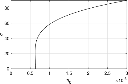
Figure 8: SNIC bifurcation curve of a fixed point of (40)-(41). A stable fixed point exists to the left of the curve and stable periodic oscillations to the right. Parameters: $\Delta=0.01,g=0.4,\langle k\rangle=100$, $P(k)$ is a uniform distribution on $[100-\sigma,100+\sigma]$.

Now consider a more heterogeneous network with $\Delta=0.05$ and $\eta_{0}=0.2$, i.e. well above threshold so that most neurons would fire if uncoupled, again with $\langle k\rangle=100$ and a uniform degree distribution on $[100-\sigma,100+\sigma]$. Consistent with the results in piedev19 ; monpaz20 we find that upon increasing $g$ (the strength of coupling) the transition to firing is through a Hopf bifurcation, as shown in Fig. 9. Increasing the width of the degree distribution decreases the value of $g$ at which collective oscillations start. This bifurcation is reminiscent of that which occurs in all-to-all connected networks of Winfree oscillators win67 : increasing the coupling strength causes the onset of oscillations through a Hopf bifurcation pazmon13 ; galmon17 ; laibla21 . As is also seen in networks of Winfree oscillators, decreasing $\Delta$ (the level of heterogeneity) has the same effect as increasing $g$, producing oscillations via a Hopf bifurcation (not shown).

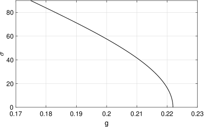
Figure 9: Hopf bifurcation curve of a fixed point of (40)-(41). A stable fixed point exists to the left and stable periodic oscillations to the right. Parameters: $\Delta=0.05,\langle k\rangle=100,\eta_{0}=0.2$, $P(k)$ is uniform distribution on $[100-\sigma,100+\sigma]$.

We tried to reproduce the trend in Fig. 8 using a network of gap junction coupled Morris-Lecar neurons, the equations of which are given in Appendix A. We chose the $I_{i}$ from a Lorentzian with HWHM $\Delta=0.01$ and coupling strength $\epsilon=0.3$. We were unable to reproduce the trend. This is likely due to the sensitivity of the network to the value of $I_{0}$: notice the very small range of $\eta_{0}$ values in Fig. 8. The variation in values of $I_{0}$ at which the bifurcation occured between different networks (with different $\sigma$) was too large to determine any significant trend.

However, we can reproduce the movement of the Hopf bifurcation as $\sigma$ is varied in a network of Morris-Lecar neurons; see Fig. 9. We consider $N=2500$ and $\langle k\rangle=100$ with a uniform degree distribution on $[100-\sigma,100+\sigma]$. We obtain evidence of a supercritical Hopf bifurcation as $\epsilon$ is increased as shown in Fig. 10. On the vertical axis we plot the standard deviation of $\hat{s}$ over a period of 10 seconds, having discarded the first 10 seconds as transients. As expected, increasing $\sigma$ decreases the value of $g$ at which the bifurcation occurs.

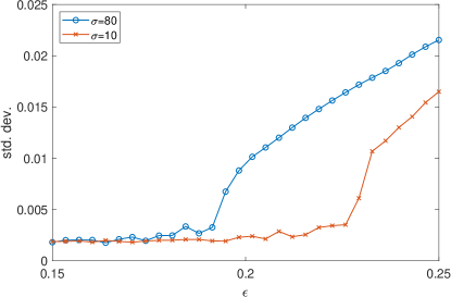
Figure 10: Evidence of a supercritical Hopf bifurcation in a network of gap-junction coupled Morris-Lecar neurons. On the vertical axis we plot the standard deviation of $\hat{s}$ (the mean of the $s_{i}$) over a period of 10 seconds, having discarded the first 10 seconds as transients.

IV Gaussian or uniform distribution of $\eta_{i}$

All of the results so far have involved a Lorentzian distribution of a heterogeneous parameter, either the input currents to theta neurons or to Morris-Lecar neurons. In this section we investigate whether we obtain qualitatively similar results for other distributions.

Using either a Gaussian or uniform distribution of $I_{i}$ in a Morris-Lecar network we obtained qualitatively the same results as in Figs. 4 and 7 for synaptic coupling (results not shown). We investigated the effects shown in Fig. 8 in a network of gap-junction coupled Morris-Lecar neurons for both uniform and normally distributed $I_{i}$. The results are shown in Fig. 11. For each value of $\sigma$ we created a network and a realisation of the $I_{i}$, and then used bisection in $I_{0}$ to approximately determine the transition from quiescence to periodic firing (with large period). For broader distributions (panel (a)) we obtained the same trend as in Fig. 8 while for narrower distributions we seem to obtain the opposite trend (panel (b)). Note that the theshold for firing for a single neuron is $I_{0}\approx 39.693455$, so all bifurcations occur for $I_{0}$ less than this, in contrast with the results in Fig. 8. Such an effect has been seen before in excitable systems lafcol10 indicating that the Lorentzian distribution of heterogeneity, while providing analytical insight, may not give generic results.

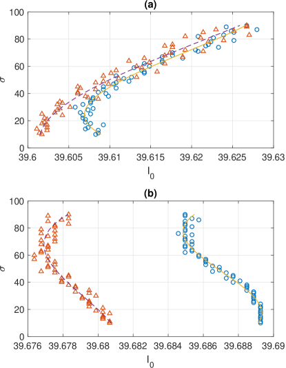
Figure 11: SNIC bifurcations for gap-junction coupled Morris-Lecar neurons. (a): $I_{i}$ chosen from a uniform distribution on $[-1/2,1/2]$ (blue circles, solid curve) or a normal distribution with centre zero and standard deviation $1/3$ (red triangle, dashed curve). (b): $I_{i}$ chosen from a uniform distribution on $[-1/8,1/8]$ (blue circles, solid curve) or a normal distribution with centre zero and standard deviation $1/10$ (red triangle, dashed curve). The curves result from fitting the values of $I_{0}$ as a cubic function of $\sigma$ and are to guide the eye. Parameters: $N=2500,\epsilon=0.3$.

We reproduced the results in Fig. 9 with the $I_{i}$ taken from a unit Gaussian (normal distribution), as shown in Fig. 12(a). Choosing the $I_{i}$ from a uniform distribution on $[-1,1]$ we obtain the results in Fig. 12(b). Quasistatically sweeping $\epsilon$ up and down for $\sigma=10$ we found a region of bistability between an approximate steady state and a macroscopic oscillation, suggesting that the Hopf bifurcation seen is subcritical. For clarity, we only show the results of increasing $\epsilon$ for both networks. The effect of varying the width of the in-degree distribution is the same: broadening the distribution moves the Hopf bifurcation to a lower value of $\epsilon$.

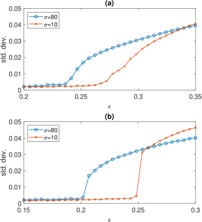
Figure 12: Evidence of Hopf bifurcations in networks of gap-junction coupled Morris-Lecar neurons. (a): $I_{i}$ taken from a unit Gaussian distribution. The Hopf bifurcations appear to be supercritical. (b): $I_{i}$ taken from a uniform distribution on $[-1,1]$. The Hopf bifurcation for $\sigma=10$ appears to be subcritical, as explained in the text. For each panel, on the vertical axis we plot the standard deviation of $\hat{s}$ (the mean of the $s_{i}$) over a period of 10 seconds, having discarded the first 10 seconds as transients. $N=2500$.

V Summary

We have derived approximate equations describing the expected dynamics of large networks of theta neurons, under the assumption that the heterogeneous parameter has a Lorentzian distribution. We have chosen the case of neutral assorativity within the networks and independent in- and out-degrees, concentrating on the effects of varying the widths of the in- and out-degree distributions. We have investigated both synaptic and gap junctional coupling. Numerical bifurcation analysis has enabled us to determine the effects of varying the degree distributions on the networks’ dynamics.

For synaptically coupled inhibitory neurons, broadening the in-degree distribution destroys macroscopic oscillations while for excitatory networks, it narrows the range of values of mean input for which the network is bistable. The dynamics are independent of the out-degree distribution. For gap junctional coupling, broadening the degree distribution causes SNIC or Hopf bifurcations associated with the onset of collective firing to move in parameter space. Most of the results are confirmed to occur in networks of more realistic neurons with different distributions of heterogeneity, but the use of Lorentzian distributions may not always give generic results.

This work could be generalised in several ways. One is to extend it to cover coupled populations of excitatory and inhibitory neurons rox11 ; coobyr19 ; lai17 . This would naturally result in more parameters to explore, as distributions of degrees relating to up to four types of connection would need to be specified. Another area of interest is the inclusion of noise in the neurons’ dynamics. Noise is known to play a significant role in neural dynamics lailor09 ; ermter10 yet its presence would invalidate the use of the Ott/Antonsen ansatz which lies behind the derivations in this paper. Goldobin et al. have made progress in this area, developing perturbation theory away from noise-free case tyugol18 ; goldol20 ; goldiv21 ; goltyu18 ; goldol19 , and Ratas and Pyragas have applied these ideas to networks of theta neurons ratpyr19 .

Acknowledgement: This work was partially supported by the Marsden Fund Council from Government funding, managed by Royal Society Te Aparangi, grant number 17-MAU-054.

Appendix A Morris-Lecar equations

A.1 Synaptic coupling

For synaptic coupling the equations for $N$ neurons are

$$C\frac{dV_{i}}{dt} =g_{L}(V_{L}-V_{i})+g_{Ca}m_{\infty}(V_{i})(V_{Ca}-V_{i})$$ (45)

$$+g_{K}n_{i}(V_{K}-V_{i})+I_{0}+I_{i}+\frac{\epsilon}{\langle k\rangle}\sum_{j=1}^{N}A_{ij}s_{j}$$

$$\frac{dn_{i}}{dt} =\frac{\lambda_{0}(w_{\infty}(V_{i})-n_{i})}{\tau_{n}(V_{i})}$$ (46)

$$\tau\frac{ds_{i}}{dt} =s_{\infty}(V_{i})-s_{i}$$ (47)

where

$$m_{\infty}(V) =0.5(1+\tanh{[(V-V_{1})/V_{2}]})$$ (48)

$$w_{\infty}(V) =0.5(1+\tanh{[(V-V_{3})/V_{4}]})$$ (49)

$$\tau_{n}(V) =\frac{1}{\cosh{[(V-V_{3})/(2V_{4})]}}$$ (50)

$$s_{\infty}(V) =1+\tanh{(V/10)}.$$ (51)

Parameters are $V_{1}=-1.2,V_{2}=18,V_{3}=12,V_{4}=17.4,\lambda_{0}=1/15msec^{-1},g_{L}=2,g_{K}=8,g_{Ca}=4,V_{L}=-60,V_{Ca}=120,V_{K}=-80,C=20\mu F/cm^{2}$ and these are unchanged throughout the paper. Voltages are in mV and conductances are in $mS/cm^{2}$. These are taken from tsukit06 but we have added synaptic dynamics. The theshold for firing for single neuron is $I_{0}\approx 39.693455$.

For Fig. 4 we set $\epsilon=-1mS/cm^{2},I_{0}=41$. The $I_{i}$ were taking from a Lorentzian with mean zero and HWHM $0.01$. For Fig. 7 we set $\epsilon=25mS/cm^{2},\tau=20,N=500$. The $I_{i}$ were taking from a Lorentzian with mean zero and HWHM $0.01$.

A.2 Gap junction coupling

For gap-junctional coupling we use

$$C\frac{dV_{i}}{dt} =g_{L}(V_{L}-V_{i})+g_{Ca}m_{\infty}(V_{i})(V_{Ca}-V_{i})$$

$$+g_{K}n_{i}(V_{K}-V_{i})+I_{0}+I_{i}$$

$$+\frac{\epsilon}{\langle k\rangle}\sum_{j=1}^{N}A_{ij}(V_{j}-V_{i})$$ (52)

$$\frac{dn_{i}}{dt} =\frac{\lambda_{0}(w_{\infty}(V_{i})-n_{i})}{\tau_{n}(V_{i})}$$ (53)

where $m_{\infty}(V),w_{\infty}(V)$ and $\tau_{n}(V)$ and all other parameters are as above. For Fig. 10 we set $I_{0}=40$ and choose the $I_{i}$ from a Lorentzian with mean zero and HWHM 0.5.

References

- (1) A. Roxin, “The role of degree distribution in shaping the dynamics in networks of sparsely connected spiking neurons,” Frontiers in Computational Neuroscience, vol. 5, p. 8, 2011.
- (2) C. Schmeltzer, A. H. Kihara, I. M. Sokolov, and S. Rüdiger, “Degree correlations optimize neuronal network sensitivity to sub-threshold stimuli,” PloS one, vol. 10, no. 6, p. e0121794, 2015.
- (3) D. Q. Nykamp, D. Friedman, S. Shaker, M. Shinn, M. Vella, A. Compte, and A. Roxin, “Mean-field equations for neuronal networks with arbitrary degree distributions,” Phys. Rev. E, vol. 95, p. 042323, Apr 2017.
- (4) M. B. Martens, A. R. Houweling, and P. H. Tiesinga, “Anti-correlations in the degree distribution increase stimulus detection performance in noisy spiking neural networks,” Journal of Computational Neuroscience, vol. 42, no. 1, pp. 87–106, 2017.
- (5) V. Pernice, M. Deger, S. Cardanobile, and S. Rotter, “The relevance of network micro-structure for neural dynamics,” Frontiers in Computational Neuroscience, vol. 7, p. 72, 2013.
- (6) G. B. Ermentrout and D. H. Terman, Mathematical Foundations of Neuroscience, vol. 35 of Interdisciplinary Applied Mathematics. Springer, 2010.
- (7) M. V. Bennett and R. Zukin, “Electrical coupling and neuronal synchronization in the mammalian brain,” Neuron, vol. 41, no. 4, pp. 495 – 511, 2004.
- (8) B. Ermentrout, “Gap junctions destroy persistent states in excitatory networks,” Physical Review E, vol. 74, no. 3, p. 031918, 2006.
- (9) C. R. Laing and C. Bläsche, “The effects of within-neuron degree correlations in networks of spiking neurons,” Biological Cybernetics, vol. 114, pp. 337–347, 2020.
- (10) M. D. LaMar and G. D. Smith, “Effect of node-degree correlation on synchronization of identical pulse-coupled oscillators,” Physical Review E, vol. 81, no. 4, p. 046206, 2010.
- (11) J. Vasquez, A. Houweling, and P. Tiesinga, “Simultaneous stability and sensitivity in model cortical networks is achieved through anti-correlations between the in- and out-degree of connectivity,” Frontiers in Computational Neuroscience, vol. 7, p. 156, 2013.
- (12) M. Vegué and A. Roxin, “Firing rate distributions in spiking networks with heterogeneous connectivity,” Phys. Rev. E, vol. 100, p. 022208, Aug 2019.
- (13) C. Bläsche, S. Means, and C. R. Laing, “Degree assortativity in networks of spiking neurons,” Journal of Computational Dynamics, vol. 7, pp. 401–423, 2020.
- (14) M. Kähne, I. Sokolov, and S. Rüdiger, “Population equations for degree-heterogenous neural networks,” Physical Review E, vol. 96, no. 5, p. 052306, 2017.
- (15) S. De Franciscis, S. Johnson, and J. Torres, “Enhancing neural-network performance via assortativity,” Physical Review E - Statistical, Nonlinear, and Soft Matter Physics, vol. 83, no. 3, 2011. cited By 19.
- (16) E. Ott and T. Antonsen, “Low dimensional behavior of large systems of globally coupled oscillators,” Chaos, vol. 18, p. 037113, 2008.
- (17) E. Ott and T. Antonsen, “Long time evolution of phase oscillator systems,” Chaos, vol. 19, p. 023117, 2009.
- (18) C. R. Laing, “Derivation of a neural field model from a network of theta neurons,” Physical Review E, vol. 90, no. 1, p. 010901, 2014.
- (19) C. R. Laing, “The dynamics of chimera states in heterogeneous Kuramoto networks,” Physica D, vol. 238, pp. 1569–1588, 2009.
- (20) T. B. Luke, E. Barreto, and P. So, “Complete classification of the macroscopic behavior of a heterogeneous network of theta neurons,” Neural Computation, vol. 25, pp. 3207–3234, 2013.
- (21) J. G. Restrepo and E. Ott, “Mean-field theory of assortative networks of phase oscillators,” EPL (Europhysics Letters), vol. 107, no. 6, p. 60006, 2014.
- (22) S. Chandra, D. Hathcock, K. Crain, T. M. Antonsen, M. Girvan, and E. Ott, “Modeling the network dynamics of pulse-coupled neurons,” Chaos, vol. 27, no. 3, p. 033102, 2017.
- (23) L. Tattini, S. Olmi, and A. Torcini, “Coherent periodic activity in excitatory erdös-renyi neural networks: the role of network connectivity,” Chaos: An Interdisciplinary Journal of Nonlinear Science, vol. 22, no. 2, p. 023133, 2012.
- (24) A. V. Goltsev, F. V. de Abreu, S. N. Dorogovtsev, and J. F. F. Mendes, “Stochastic cellular automata model of neural networks,” Phys. Rev. E, vol. 81, p. 061921, Jun 2010.
- (25) S. Song, P. J. Sjöström, M. Reigl, S. Nelson, and D. B. Chklovskii, “Highly nonrandom features of synaptic connectivity in local cortical circuits,” PLoS Biol, vol. 3, no. 3, p. e68, 2005.
- (26) Y.-M. Qin, Y.-Q. Che, and J. Zhao, “Effects of degree distributions on signal propagation in noisy feedforward neural networks,” Physica A: Statistical Mechanics and its Applications, vol. 512, pp. 763–774, 2018.
- (27) S. Coombes and Á. Byrne, “Next generation neural mass models,” in Nonlinear dynamics in computational neuroscience, pp. 1–16, Springer, 2019.
- (28) B. Ermentrout, “Type I membranes, phase resetting curves, and synchrony,” Neural Computation, vol. 8, no. 5, pp. 979–1001, 1996.
- (29) C. Börgers, An introduction to modeling neuronal dynamics, vol. 66. Springer, 2017.
- (30) C. Laing, C. Bläsche, and S. Means, “Dynamics of structured networks of winfree oscillators,” Frontiers in Systems Neuroscience, vol. 15, p. 7, 2021.
- (31) C. R. Laing, “Exact neural fields incorporating gap junctions,” SIAM Journal on Applied Dynamical Systems, vol. 14, no. 4, pp. 1899–1929, 2015.
- (32) E. Montbrió, D. Pazó, and A. Roxin, “Macroscopic description for networks of spiking neurons,” Physical Review X, vol. 5, no. 2, p. 021028, 2015.
- (33) M. Newman, “The structure and function of complex networks,” SIAM Review, vol. 45, no. 2, pp. 167–256, 2003.
- (34) K. Tsumoto, H. Kitajima, T. Yoshinaga, K. Aihara, and H. Kawakami, “Bifurcations in morris–lecar neuron model,” Neurocomputing, vol. 69, no. 4-6, pp. 293–316, 2006.
- (35) C. R. Laing and A. Longtin, “Dynamics of deterministic and stochastic paired excitatory—inhibitory delayed feedback,” Neural computation, vol. 15, no. 12, pp. 2779–2822, 2003.
- (36) M. Galarreta and S. Hestrin, “A network of fast-spiking cells in the neocortex connected by electrical synapses,” Nature, vol. 402, no. 6757, pp. 72–75, 1999.
- (37) S. Ostojic, N. Brunel, and V. Hakim, “Synchronization properties of networks of electrically coupled neurons in the presence of noise and heterogeneities,” Journal of computational neuroscience, vol. 26, no. 3, p. 369, 2009.
- (38) R. D. Traub, N. Kopell, A. Bibbig, E. H. Buhl, F. E. LeBeau, and M. A. Whittington, “Gap junctions between interneuron dendrites can enhance synchrony of gamma oscillations in distributed networks,” Journal of Neuroscience, vol. 21, no. 23, pp. 9478–9486, 2001.
- (39) P. E. Latham, B. Richmond, P. Nelson, and S. Nirenberg, “Intrinsic dynamics in neuronal networks. i. theory,” Journal of neurophysiology, vol. 83, no. 2, pp. 808–827, 2000.
- (40) G. B. Ermentrout and N. Kopell, “Parabolic bursting in an excitable system coupled with a slow oscillation,” SIAM Journal on Applied Mathematics, vol. 46, no. 2, pp. 233–253, 1986.
- (41) E. Montbrió and D. Pazó, “Exact mean-field theory explains the dual role of electrical synapses in collective synchronization,” Physical Review Letters, vol. 125, no. 24, p. 248101, 2020.
- (42) B. Pietras, F. Devalle, A. Roxin, A. Daffertshofer, and E. Montbrió, “Exact firing rate model reveals the differential effects of chemical versus electrical synapses in spiking networks,” Physical Review E, vol. 100, no. 4, p. 042412, 2019.
- (43) Á. Byrne, J. Ross, R. Nicks, and S. Coombes, “Mean-field models for eeg/meg: from oscillations to waves,” bioRxiv, 2020.
- (44) L. F. Lafuerza, P. Colet, and R. Toral, “Nonuniversal results induced by diversity distribution in coupled excitable systems,” Physical review letters, vol. 105, no. 8, p. 084101, 2010.
- (45) S. Shinomoto and Y. Kuramoto, “Phase Transitions in Active Rotator Systems,” Progress of Theoretical Physics, vol. 75, pp. 1105–1110, 05 1986.
- (46) L. M. Childs and S. H. Strogatz, “Stability diagram for the forced Kuramoto model,” Chaos, vol. 18, no. 4, p. 043128, 2008.
- (47) C. Zheng and A. Pikovsky, “Stochastic bursting in unidirectionally delay-coupled noisy excitable systems,” Chaos: An Interdisciplinary Journal of Nonlinear Science, vol. 29, no. 4, p. 041103, 2019.
- (48) O. Omel’chenko, M. Wolfrum, and C. R. Laing, “Partially coherent twisted states in arrays of coupled phase oscillators,” Chaos, vol. 24, no. 2, p. 023102, 2014.
- (49) S. Strogatz, “From Kuramoto to Crawford: exploring the onset of synchronization in populations of coupled oscillators,” Physica D, vol. 143, pp. 1–20, 2000.
- (50) D. M. Abrams, R. Mirollo, S. H. Strogatz, and D. A. Wiley, “Solvable model for chimera states of coupled oscillators,” Physical Review Letters, vol. 101, p. 084103, 2008.
- (51) A. T. Winfree, “Biological rhythms and the behavior of populations of coupled oscillators,” Journal of Theoretical Biology, vol. 16, no. 1, pp. 15–42, 1967.
- (52) D. Pazó and E. Montbrió, “Low-dimensional dynamics of populations of pulse-coupled oscillators,” Physical Review X, vol. 4, p. 011009, 2014.
- (53) R. Gallego, E. Montbrió, and D. Pazó, “Synchronization scenarios in the winfree model of coupled oscillators,” Phys. Rev. E, vol. 96, p. 042208, Oct 2017.
- (54) C. R. Laing, “Phase oscillator network models of brain dynamics,” in Computational models of brain and behavior, pp. 505–517, Wiley Online Library, 2017.
- (55) C. Laing and G. J. Lord, eds., Stochastic methods in neuroscience. Oxford University Press, 2009.
- (56) I. V. Tyulkina, D. S. Goldobin, L. S. Klimenko, and A. Pikovsky, “Dynamics of noisy oscillator populations beyond the ott-antonsen ansatz,” Physical review letters, vol. 120, no. 26, p. 264101, 2018.
- (57) D. S. Goldobin and A. V. Dolmatova, “Circular cumulant reductions for macroscopic dynamics of kuramoto ensemble with multiplicative intrinsic noise,” Journal of Physics A: Mathematical and Theoretical, vol. 53, no. 8, p. 08LT01, 2020.
- (58) D. S. Goldobin, M. di Volo, and A. Torcini, “A reduction methodology for fluctuation driven population dynamics,” 2021.
- (59) D. S. Goldobin, I. V. Tyulkina, L. S. Klimenko, and A. Pikovsky, “Collective mode reductions for populations of coupled noisy oscillators,” Chaos: An Interdisciplinary Journal of Nonlinear Science, vol. 28, no. 10, p. 101101, 2018.
- (60) D. S. Goldobin and A. V. Dolmatova, “Ott-Antonsen ansatz truncation of a circular cumulant series,” Physical Review Research, vol. 1, no. 3, p. 033139, 2019.
- (61) I. Ratas and K. Pyragas, “Noise-induced macroscopic oscillations in a network of synaptically coupled quadratic integrate-and-fire neurons,” Physical Review E, vol. 100, no. 5, p. 052211, 2019.