Adversarial Inverse Reinforcement Learning for Mean Field Games

Abstract

Mean field games (MFGs) provide a mathematically tractable framework for modelling large-scale multi-agent systems by leveraging mean field theory to simplify interactions among agents. It enables applying inverse reinforcement learning (IRL) to predict behaviours of large populations by recovering reward signals from demonstrated behaviours. However, existing IRL methods for MFGs are powerless to reason about uncertainties in demonstrated behaviours of individual agents. This paper proposes a novel framework, Mean-Field Adversarial IRL (MF-AIRL), which is capable of tackling uncertainties in demonstrations. We build MF-AIRL upon maximum entropy IRL and a new equilibrium concept. We evaluate our approach on simulated tasks with imperfect demonstrations. Experimental results demonstrate the superiority of MF-AIRL over existing methods in reward recovery.

1 Introduction

Pioneered by the work of (Huang et al., 2006) and (Lasry and Lions, 2007), the paradigm of mean field games (MFGs) facilitates reinforcement learning (RL) in large-scale multi-agent systems, which is otherwise intractable due to the curse of dimensionality and the explosion of agent interactions (Yang et al., 2018b). Through mean field approximation, MFGs reduce the interactions among agents to those between a single individual agent and the mean field, a virtual agent that represents aggregated behaviours of the population at large. The interplay between individual and population gives rise to the conventional solution concept for MFGs, mean field Nash equilibrium (MFNE), which stipulates bidirectional constraints between the two sides: every agent’s policy maximises its rewards given the mean field and, in turn, the mean field is uniquely resulted by each agent’s policy. Aiming at computing an MFNE or its variants, RL for MFGs has been applied to large-scale multi-agent scenarios such as pricing in large-scale markets (Subramanian and Mahajan, 2019), auctions with many bidders (Guo et al., 2019) and infection spread modelling (Lee et al., 2021). However, RL for MFGs depends crucially on a well-designed reward function, but manually tuning reward functions can be challenging in the real-world. In MFGs, since an agent’s reward depends not only on its own action but on the population’s mean field, how to obtain a reward function is a very challenging question.

Inverse reinforcement learning (IRL) (Ng and Russell, 2000) provides a powerful framework for predicting agent behaviours via acquiring suitable reward signals from expert demonstrations. For MFGs, IRL remains largely unexplored, albeit there are two recent attempts. Yang et al. (2018a) first proposed a centralised IRL method for MFGs by showing that an MFG can be reduced to a Markov decision process (MDP) that describes the population’s collective actions and average rewards; they thus applied single-agent IRL methods on top of this MDP. Subsequently, Chen et al. (2022) revealed that this reduction holds only if the MFNE is socially optimal, i.e., it maximises the population’s average rewards; they thus framed the problem at the decentralised setting, i.e., inferring the reward function for an individual agent from demonstrations provided by individual experts instead of by the population. They put forward Mean Field IRL (MFIRL) based on margin optimisation (Ratliff et al., 2006), a more general approach effective for both socially optimal and ordinary MFNE.

However, MFIRL is still limited in terms of practical use. First, due to limited cognitive or computational capability, an agent often has bounded rationality in real-life, i.e., choosing satisfactory rather than optimal actions (Harstad and Selten, 2013). Consequently, the resulting demonstrations possess uncertainties in general. For example, a customer in a restaurant orders an acceptable dish which is not necessarily his favourite as he is rush in time. MFIRL is unable to reason about such uncertainties in demonstrations as agents in MFNE are assumed to never take suboptimal behaviours. This makes MFIRL unsuitable for situations where bounded rationality of agents is observed. Then, since an MFNE is not unique in general (Cui and Koeppl, 2021), the behaviour predicted by MFIRL can be under-specified as it does not guarantee to elicit a unique policy from a learned reward function. In this sense, from an application standpoint, MFIRL is also not useful for behaviour prediction.

Towards a practical IRL method for MFGs, we invoke the idea of Maximum Entropy IRL (MaxEnt IRL) (Ziebart et al., 2008). MaxEnt IRL provides a general probabilistic framework to tackle demonstrations with uncertainties. It assumes that the expert policy maximises the entropy, as a measure of uncertainties, of the demonstrated trajectory distribution in terms of rewards; it thus allows us to find a reward function that rationalises expert demonstrations with the least commitment. Moreover, since a policy leading to the maximum entropy trajectory distribution is unique given a reward function, MaxEnt IRL is more useful for behaviour prediction. However, MaxEnt IRL is inefficient as it requires iteratively computing a partition function for the trajectory distribution while tuning a reward function. Fortunately, Adversarial IRL (AIRL) was proposed as an efficient approximation to MaxEnt IRL Finn et al. (2016); Fu et al. (2018), which frames a sampling-based approximation of MaxEnt IRL as optimising a generative adversarial network (Goodfellow et al., 2014). To recover reward functions for large-scale multi-agent systems from demonstrations with uncertainties, we thus hope to transfer the concept of MaxEnt IRL to MFGs.

However, extending MaxEnt IRL is challenging. First, because MFNE assumes agents never take suboptimal behaviours, it is incompatible with MaxEnt IRL in the sense that it cannot provide a trajectory distribution which can be used for the probabilistic reward inference. Second, since in MFGs the individual and population dynamics are intertwined (the policy and mean field are interdependent), the trajectory distribution will depend on the mean field which is intractable to analytically express in terms of rewards. Consequently, even if we have a compatible solution concept, the coupling between individual and population dynamics would prevent us from performing probabilistic inference for the reward function.

The primary contribution of this paper lies in the proposal of a new probabilistic IRL framework, Mean-Field Adversarial IRL (MF-AIRL), for MFGs. MF-AIRL integrates ideas from decentralised IRL for MFGs, MaxEnt IRL, and generative adversarial learning into a unified probabilistic model for reward inferences in large-scale problems. We summarise specific contributions as follows: (1) We build MF-AIRL upon a new equilibrium concept termed entropy-regularised MFNE (ERMFNE) (see Sec. 3). We show that ERMFNE can characterise an individual’s trajectory distribution induced by a reward function in a principled way (see Theorem 3). (2) Taking ERMFNE as the solution concept, we extend MaxEnt IRL to MFGs (see Sec. 4). We approximately decouple individual and population dynamics by determining the mean field as the empirical value estimated from demonstrations (see Theorem 4). (3) By using generative adversarial learning to efficiently solve MaxEnt IRL in MFGs, we develop the practical MF-AIRL framework (see Sec. 5). (4) We evaluate MF-AIRL on simulated tasks (see Sec. 6). Results show the outperformance of MF-AIRL over existing methods in reward recovery.

2 Preliminaries

This section introduces mean field games (MFGs) and the maximum entropy inverse reinforcement learning (MaxEnt IRL) framework. The marriage of the two gives rise to our proposed approach to modelling and predicting behaviours of a large population of agents.

2.1 Mean Field Games

Following the conventional MFG model in the learning setting, we focus on MFGs with finite state and action spaces and more generally a finite time horizon (Elie et al., 2020). Consider an $N$-player symmetric game, i.e., all agents share the same local state space ${{\mathcal{S}}}$, action space ${{\mathcal{A}}}$, and a reward function that is invariant under the permutation of identities of agents without changing their states and actions. Let $(s^{1},\ldots,s^{N})\in{{\mathcal{S}}}^{N}$ denote a joint state, where $s^{i}\in{{\mathcal{S}}}$ is the state of the $i$th agent. As $N$ grows large, the game becomes intractable to analyse due to the curse of dimensionality. MFGs achieve tractability by considering the asymptotic limit when $N$ approaches infinity. Formally, take the limit as $N\to\infty$. Due to the homogeneity of agents, MFGs use an empirical distribution $\mu\in{{\mathcal{P}}}({{\mathcal{S}}})$, called a mean field, to represent the statistical information of the joint state:

$$\mu(s)\triangleq\lim_{N\to\infty}\frac{1}{N}\sum_{i=1}^{N}\mathds{1}_{\{s^{i}=s\}}.$$

Here, ${{\mathcal{P}}}({{\mathcal{S}}})$ represents the set all probability measures over ${{\mathcal{S}}}$ and $\mathds{1}$ denotes the indicator function, i.e., $\mathds{1}_{x}=1$ if $x$ is true and $0$ otherwise. The transition function $P\colon{{\mathcal{S}}}\times{{\mathcal{A}}}\times{{\mathcal{P}}}({{\mathcal{S}}})\times{{\mathcal{P}}}({{\mathcal{S}}})\to[0,1]$ specifies how states evolve, i.e., an agent transits to the next state $s_{t+1}$ with the probability $P(s_{t+1}|s_{t},a_{t},\mu_{t})$. Let $T\in\mathbb{N}^{+}$ denote a finite time horizon. A mean field flow (MF flow for short) thus consists of a sequence of $T+1$ mean fields ${\bm{\mu}}\triangleq\{\mu_{t}\}_{t=0}^{T}$. The initial mean field $\mu_{0}$ is given. The running reward at each step is determined by a bounded reward function $r\colon{{\mathcal{S}}}\times{{\mathcal{A}}}\times{{\mathcal{P}}}({{\mathcal{S}}})\rightarrow\mathbb{R}$. Let $\tau\triangleq\{(s_{t},a_{t})\}_{t=0}^{T}$ denote a state-action trajectory of an agent. We write an agent’s long-term reward under a given MF flow ${\bm{\mu}}$ as $R(\tau)\triangleq\sum_{t=0}^{T-1}r(s_{t},a_{t},\mu_{t})$. As a summary, an MFG is defined as a tuple $({{\mathcal{S}}},{{\mathcal{A}}},P,\mu_{0},r)$.

A time-varying stochastic policy ${\bm{\pi}}\triangleq\{\pi_{t}\}_{t=0}^{T}$ is adopted to characterise a strategic agent, where each $\pi_{t}\colon{{\mathcal{S}}}\rightarrow{{\mathcal{P}}}({{\mathcal{A}}})$ is the per-step policy, i.e., an agent chooses actions following $a_{t}\sim\pi_{t}(\cdot|s)$. Given an MF flow ${\bm{\mu}}$ and a policy ${\bm{\pi}}$, an agent’s expected return (cumulative rewards) is written as

$$J({\bm{\mu}},{\bm{\pi}})\triangleq\mathbb{E}_{\tau\sim({\bm{\mu}},{\bm{\pi}})}\left[R(\tau)\right],$$ (1)

where $s_{0}\sim\mu_{0},a_{t}\sim\pi_{t}(\cdot|s_{t}),s_{t+1}\sim P(\cdot|s_{t},a_{t},\mu_{t}).$

2.2 Mean Field Nash Equilibrium

Fixing an MF flow ${\bm{\mu}}$, a policy ${\bm{\pi}}$ is called a best response to ${\bm{\mu}}$ if it maximises $J({\bm{\mu}},{\bm{\pi}})$. We denote the set of all best-response policies to ${\bm{\mu}}$ by $\Psi({\bm{\mu}})\triangleq\operatorname*{arg\,max}_{{\bm{\pi}}}J({\bm{\mu}},{\bm{\pi}})$. However, since all agents optimise their policies simultaneously, the MF flow would shift. The solution thus needs to consider how an agent’s policy affects the population’s MF flow. Due to the homogeneity of agents, at optimality, everyone would follow the same policy. The dynamics of the MF flow can thus be governed by the (discrete-time) McKean-Vlasov (MKV) equation (Carmona et al., 2013):

$$\mu_{t+1}(s^{\prime})=\sum_{s\in{{\mathcal{S}}}}\mu_{t}(s)\sum_{a\in{{\mathcal{A}}}}\pi_{t}(a|s)\;P(s^{\prime}|s,a,\mu_{t}).$$ (2)

Given a policy ${\bm{\pi}}$, denote ${\bm{\mu}}=\Phi({\bm{\pi}})$ as the MF flow that fulfils MKV equation. We say ${\bm{\mu}}$ is consistent with ${\bm{\pi}}$ if ${\bm{\mu}}=\Phi({\bm{\pi}})$. This consistency guarantees that the state marginal distribution flow of a single agent matches the MF flow at the population level. The conventional solution concept for MFGs is the mean field Nash equilibrium (MFNE).

Definition 1

A pair $({\bm{\mu}}^{\star},{\bm{\pi}}^{\star})$ is called a mean field Nash equilibrium if it satisfies: (1) Agent rationality: ${\bm{\pi}}^{\star}\in\Psi({\bm{\mu}}^{\star})$; (2) Population consistency: ${\bm{\mu}}^{\star}=\Phi({\bm{\pi}}^{\star})$.

Shown by (Cui and Koeppl, 2021), if $r(s,a,\mu)$ and $P(s^{\prime}|s,a,\mu)$ are continuous, an MFNE is guaranteed to exist but it may not exist uniquely.

2.3 Maximum Entropy IRL

We next give an overview of MaxEnt IRL (Ziebart et al., 2008, 2010) in the context of an MDP defined by a tuple $({{\mathcal{S}}},{{\mathcal{A}}},P,\rho,r)$, where $r(s,a)$ is the reward function, and the environment dynamics is determined by the transition function $P(s^{\prime}|s,a)$ and initial state distribution $\rho(s)$. In (forward) reinforcement learning (RL), an optimal policy may not exist uniquely. MaxEnt RL solves this ambiguity by augmenting the expected return with a causal entropy (Ziebart et al., 2010) regularisation term ${{\mathcal{H}}}(\pi)\triangleq\mathbb{E}_{\pi}[-\log\pi(a|s)]$, i.e., the objective is to find a (stationary) policy $\pi^{\star}$ such that

$$\small\pi^{\star}=\operatorname*{arg\,max}_{\pi}\mathbb{E}_{\tau\sim\pi}\left[\sum_{t=0}^{T-1}r(s_{t},a_{t})+\beta{{\mathcal{H}}}(\pi(\cdot|s_{t}))\right],$$

where $\tau$ is a state-action trajectory sampled via $s_{0}\sim\rho_{0}$, $a_{t}\sim\pi(\cdot|s_{t})$, $s_{t+1}\sim P(\cdot|s_{t},a_{t})$ and $\beta>0$ controls relative importance of reward and entropy. Without loss of generality, it is often assumed that $\beta=1$ (Yu et al., 2019b).

Now, suppose we have no access to the reward function but have a set of demonstrated trajectories sampled from an unknown expert policy $\pi^{E}$ obtained by the above MaxEnt RL procedure. MaxEnt IRL aims to infer a reward function that rationalises expert demonstrations, which reduces to the following maximum likelihood estimation (MLE) problem:

$$p_{\omega}(\tau)\propto\rho(s_{0})\cdot\prod_{t=0}^{T-1}P(s_{t+1}|s_{t},a_{t})\cdot e^{R(\tau)},$$ (3)

$$\max_{\omega}\mathbb{E}_{\tau\sim\pi^{E}}\left[\log p_{\omega}(\tau)\right]=\mathbb{E}_{\tau\sim\pi^{E}}\left[R(\tau)\right]-\log Z_{\omega}.$$ (4)

Here, $\omega$ is the parameter of the reward function and $Z_{\omega}\triangleq\int_{\tau\sim\pi^{E}}e^{R(\tau)}d\tau$ is the partition function of Eq. (3), i.e., an integral over all feasible trajectories. Exactly computing $Z_{\omega}$ is intractable if state-action spaces are large or continuous.

Adversarial IRL (AIRL) was proposed by (Fu et al., 2018) as an efficient sampling-based approximation to MaxEnt IRL, which reframes Eq. (4) as optimising a generative adversarial network (Goodfellow et al., 2014). It uses a discriminator $D_{\omega}$ (a binary classifier) and a adaptive sampler $\pi_{\theta}$ (a policy). Particularly, the discriminator takes the following form: $D_{\omega}(s,a)=\frac{e^{f_{\omega}(s,a)}}{e^{f_{\omega}(s,a)+\pi_{\theta}(a|s)}}$, where $f_{\omega}$ serves as the parameterised reward function. The update of $D_{\omega}$ is interleaved with the update of $\pi_{\theta}$: $D_{\omega}$ is trained to update the reward function by distinguishing between the trajectories sampled from the expert and the adaptive sampler; while $\pi_{\theta}$ is trained to maximise $\mathbb{E}_{\tau\sim\pi_{\theta}}\left[\sum_{t=0}^{T-1}\log D_{\omega}(s_{t},a_{t})-\log(1-D_{\omega}(s_{t},a_{t}))\right]$.

IRL faces the ambiguity of reward shaping (Ng et al., 1999), i.e., multiple reward functions can induce the same optimal policy. To mitigate this ambiguity, Fu et al. (2018) further restrict the parameterised reward in $D_{\omega}$ to a specific structure by supplying a state-only potential-based reward shaping function $h_{\phi}:{{\mathcal{S}}}\to\mathbb{R}$:

$$f_{\omega,\phi}(s_{t},a_{t},s_{t+1})=r_{\omega}(s_{t},a_{t})+h_{\phi}(s_{t+1})-h_{\phi}(s_{t}).$$

As shown in (Fu et al., 2018, Theorem C.1), under certain conditions, $r_{\omega}(s,a)+h_{\phi}(s)$ will recover the ground-truth reward function up to a constant.

2.4 IRL for MFGs

We adopt the general decentralised IRL setting for MFGs as in (Chen et al., 2022), which aims to infer the ground-truth reward function from demonstrations provided by individual experts. More formally, let $({{\mathcal{S}}},{{\mathcal{A}}},P,\mu_{0},r)$ be an MFG. Suppose we do not know $r(s,a,\mu)$ but have a set of $M$ expert demonstrations ${{\mathcal{D}}}_{E}=\{\tau_{j}\}_{j=1}^{M}$ sampled from an unknown equilibrium $({\bm{\mu}}^{E},{\bm{\pi}}^{E})$, where each $\tau=\{(s_{t},a_{t})\}_{t=0}^{T}$ is an individual agent’s state-action trajectory sampled via $s_{0}\sim\mu_{0}$, $a_{t}\sim\pi_{t}(\cdot|s_{t})$, $s_{t+1}\sim P(\cdot|s_{t},a_{t},\mu_{t})$. IRL for MFG asks for a reward function $r(s,a,\mu)$ under which $({\bm{\mu}}^{E},{\bm{\pi}}^{E})$ constitutes an equilibrium.

3 Entropy-Regularised MFNE

This section introduces and justifies a new solution concept for MFGs, which allows us to characterise uncertainties in agent behaviours and thereby extend MaxEnt IRL to MFGs.

3.1 A New Equilibrium Concept for MFGs

To extend MaxEnt IRL to MFGs, we need to characterise the trajectory induced by a reward function with a particular distribution as analogous to Eq. (3). However, MFNE cannot explicitly define a tractable trajectory distribution as it requires agents to never take suboptimal actions, whereas in MaxEnt IRL an expert can take sub-optimal actions with certain low probabilities. To bridge the gap between MFGs and MaxEnt IRL, we need a “soft” equilibrium concept that can characterise uncertainties in demonstrations as against MFNE being a “hard” equilibrium. To this end, a natural way in game theory is to incorporate policy entropy into rewards (Ortega and Braun, 2011; Gabaix, 2014), which enables bounded rationality, i.e, agents can take satisfactory rather than optimal actions. This inspires a new solution concept – entropy-regularised MFNE (ERMFNE) – where an agent aims to maximise the entropy-regularised rewards:

$$\tilde{J}({\bm{\mu}},{\bm{\pi}})\triangleq\mathbb{E}_{\tau\sim({\bm{\mu}},{\bm{\pi}})}\left[\sum\limits_{t=0}^{T-1}r(s_{t},a_{t},\mu_{t})+\beta{{\mathcal{H}}}(\pi_{t}(\cdot|s_{t})\right].$$

Definition 2

A pair of MF flow and policy $(\tilde{{\bm{\mu}}}^{\star},\tilde{{\bm{\pi}}}^{\star})$ is called an entropy-regularised MFNE (ERMFNE) if it satisfies: (1) Agent bounded rationality: $\tilde{J}(\tilde{{\bm{\mu}}}^{\star},\tilde{{\bm{\pi}}}^{\star})=\max_{{\bm{\pi}}}\tilde{J}(\tilde{{\bm{\mu}}}^{\star},{\bm{\pi}})$; (2) Population consistency: $\tilde{{\bm{\mu}}}^{\star}=\Phi(\tilde{{\bm{\pi}}}^{\star})$.

Despite the entropy-regularised MFGs have been studied in the literature Anahtarci et al. (2020); Guo et al. (2020); Cui and Koeppl (2021), existing works are motivated from a computational perspective, that is, entropy regularisation can improve the stability and the convergence of algorithms for computing an equilibrium. Particularly, Cui and Koeppl (2021) independently proposed a similar solution concept and showed that entropy regularisation can bring a good property of uniqueness: (1) With entropy regularisation, the best-response policy $\tilde{{\bm{\pi}}}$ to an MF flow ${\bm{\mu}}$ exists uniquely; (2) ERMFNE exists for any $\beta>0$ if $r(s,a,\mu)$ and $P(s^{\prime}|s,a,\mu)$ are continuous. Using $\tilde{{\bm{\pi}}}=\tilde{\Psi}({\bm{\mu}})$ to denote the unique best-response policy to ${\bm{\mu}}$, we obtain the the fixed point iteration for ERMFNE by alternating between ${\bm{\pi}}=\tilde{\Psi}({\bm{\mu}})$ and ${\bm{\mu}}=\Phi({\bm{\pi}})$. The fixed point iteration converges to a unique MF flow if $\beta$ is large (according to the scale of reward functions), and thereby implies a unique ERMFNE.

3.2 Trajectory Distributions Induced by ERMFNE

Note that in ERMFNE, we recover optimality (MFNE) if $\beta=0$. Although the optimality and uniqueness are approached respectively at two extermes of $\beta$, in this paper, we prioritise the property of uniqueness to ensure the well-definedness of IRL for MFGs, i.e., the expert behaviours can be interpreted with a unique equilibrium. Since we can always adjust the relative importance between rewards and entropy by scaling reward functions, following the convention in MaxEnt IRL (Fu et al., 2018; Yu et al., 2019a, b) and without loss of generality, we assume $\beta=1$ in the remainder of the analysis.

Besides uniqueness, in this paper, we take a step further to show that the entropy regularisation endows ERMFNE with the power to reason about uncertainties in expert demonstrations in a principled way. Specifically, we show that trajectory distributions induced by ERMFNE can be characterised by an energy-based model, i.e., trajectories with high expected cumulative rewards are generated with exponentially high probabilities; it can thus be used for the probabilistic inference of the underlying reward function.

Theorem 3

Let $(\tilde{{\bm{\mu}}}^{\star},\tilde{{\bm{\pi}}}^{\star})$ be the ERMFNE for an MFG $({{\mathcal{S}}},{{\mathcal{A}}},P,\mu_{0},r)$, and $D_{\mathrm{KL}}$ denote the Kullback-Leibler (KL) divergence. Then, $(\tilde{{\bm{\mu}}}^{\star},\tilde{{\bm{\pi}}}^{\star})$ is the optimal solution to the following constrained optimisation problem:

$$\min_{{\bm{\mu}},{\bm{\pi}}}D_{\mathrm{KL}}\left(p_{1}(\tau)\parallel p_{2}(\tau)\right)\text{ s.t. }{\bm{\mu}}=\Phi({\bm{\pi}})$$

$$p_{1}(\tau)=\mu_{0}(s_{0})\cdot\prod_{t=0}^{T-1}P(s_{t+1}|s_{t},a_{t},\mu_{t})\cdot\prod_{t=0}^{T}\pi_{t}(a_{t}|s_{t})$$

$$p_{2}(\tau)\propto ~{}\mu_{0}(s_{0})\cdot\prod_{t=0}^{T-1}P(s_{t+1}|s_{t},a_{t},\mu_{t})\cdot e^{R(\tau)}$$ (5)

Proof  See Appendix A.  

4 Extending MaxEnt IRL to MFGs

From now on, we assume that expert trajectories are sampled from a unique ERMFNE $({\bm{\mu}}^{E},{\bm{\pi}}^{E})$. Let $r_{\omega}(s,a,\mu)$ be an $\omega$-parameterised reward function and $({\bm{\mu}}^{\omega},{\bm{\pi}}^{\omega})$ denote the ERMFNE induced by $\omega$. Then, recovering the underlying reward function reduces to tuning $\omega$. The probability of a trajectory $\tau=\{(s_{t},a_{t})\}_{t=1}^{T}$ induced by ERMFNE with $r_{\omega}$ is defined by the following generative process:

$$p_{\omega}(\tau)=\mu_{0}(s_{0})\cdot P(s_{t+1}|s_{t},a_{t},\mu_{t}^{\omega})\cdot\prod_{t=0}^{T}\pi_{t}^{\omega}(a_{t}|s_{t}).$$ (6)

In the spirit of MaxEnt IRL, we should tune $\omega$ by maximising the likelihood of the expert trajectories with respect to the distribution defined in Eq. (6). By Theorem 3, we can instead optimise the likelihood with respect to the distribution defined in Eq. (5) as a variational approximation:

$$\max_{\omega}L(\omega) ~{}\triangleq\mathbb{E}_{\tau\sim({\bm{\mu}}^{E},{\bm{\pi}}^{E})}\Big{[}R_{\omega}(\tau)+\sum_{t=0}^{T-1}\log P(s_{t+1}|s_{t},a_{t},\mu^{\omega}_{t})\Big{]}-\log Z_{\omega},$$ (7)

where $Z_{\omega}$ is the partition function of the distribution defined in Eq. (5), i.e., an integral over all feasible trajectories:

$$Z_{\omega}\triangleq ~{}\sum_{\tau}e^{R_{\omega}(\tau)}\prod_{t=0}^{T-1}\log P(s_{t+1}|s_{t},a_{t},\mu^{\omega}_{t}).$$ (8)

However, directly optimising the likelihood objective in Eq. (7) is intractable because we cannot analytically derive the MF flow ${\bm{\mu}}^{\omega}$. This problem arises from the nature of MFGs that the policy and MF flow in ERMFNE are interdependent because $\tilde{{\bm{\pi}}}^{\star}=\tilde{\Psi}(\tilde{{\bm{\mu}}}^{\star})$ and in turn $\tilde{{\bm{\mu}}}^{\star}=\Phi(\tilde{{\bm{\pi}}}^{\star})$. This issue poses the main challenge for extending MaxEnt IRL to MFGs. Worse yet, the transition function $P$ also depends on ${\bm{\mu}}^{\omega}$, posing an extra layer of complexity as the environment dynamics is generally unknown in practice.

While, notice that if we have access to an “oracle” (known a priori) MF flow that determines the shape of the expert MF flow ${\bm{\mu}}^{E}$, an individual would be decoupled from the population. Inspired by this fact, we sidestep this problem by substituting ${\bm{\mu}}^{\omega}$ with the empirical value of ${\bm{\mu}}^{E}$, denoted by $\hat{{\bm{\mu}}}^{E}\triangleq\{\mu_{t}^{E}\}_{t=0}^{T}$, estimated from demonstrations ${{\mathcal{D}}}_{E}=\{\tau_{j}\}_{j=1}^{M}$ by calculating the occurrence frequencies of states:

$$\hat{\mu}_{t}^{E}(s)\triangleq\frac{1}{M}\sum_{j=1}^{M}\mathds{s}\mathds{1}_{\{s_{j,t}^{i}=s\}}.$$

Since the population consistency condition in ERMFNE guarantees that the state marginal distribution of a single agent matches the mean field at each time step, $\hat{{\bm{\mu}}}^{E}$ achieves an unbiased estimator of ${\bm{\mu}}^{E}$. Meanwhile, by substituting $\hat{{\bm{\mu}}}^{E}$ for ${\bm{\mu}}^{\omega}$, the transition function $P(s_{t},a_{t},\hat{\mu}_{t}^{E})$ is decoupled the from the reward parameter $\omega$ as $\hat{{\bm{\mu}}}^{E}$ does not depend on $\omega$, and henceforth being omitted in the likelihood function. Finally, with this substitution, we obtain a tractable version of the original MLE objective in Eq. (7):

$$\max_{\omega}\hat{L}\left(\omega;\hat{{\bm{\mu}}}^{E}\right)\triangleq\mathbb{E}_{\tau\sim{{\mathcal{D}}}_{E}}\left[\hat{R}_{\omega}(\tau)\right]-\log\hat{Z}_{\omega},$$ (9)

which resembles the formulation of the MLE objective of single-agent MaxEnt IRL as given in Eq. (4). Here, $\hat{R}_{\omega}(\tau)\triangleq\sum_{t=0}^{T-1}r_{\omega}(s_{t},a_{t},\hat{\mu}_{t}^{E})$ and $\hat{Z}_{\omega}\triangleq\sum_{\tau\in{{\mathcal{D}}}_{E}}e^{\hat{R}_{\omega}(\tau)}$ denotes the simplified partition function in Eq. (8).

Statistically, Eq. (9) can be interpreted as that we use a likelihood function of a “mis-specified” model that treats the policy and MF flow as being independent and replaces the MF flow with its empirical value. With this manner, we construct an estimate of the optimal solution to the original MLE problem by maximising a simplified form of the actual likelihood function defined in Eq. (7). Although we sacrifice the accuracy for achieving tractability due to the estimation error of $\hat{{\bm{\mu}}}^{E}$, we show that Eq. (9) preserves the property of the asymptotic consistency, as $\hat{{\bm{\mu}}}^{E}$ converges almost surely to ${\bm{\mu}}^{E}$ as the number of samples tends to infinity due to the law of large numbers.

Theorem 4

Let the demonstrated trajectories in ${{\mathcal{D}}}_{E}=\{\tau_{j}\}_{j=1}^{M}$ be independent and identically distributed and sampled from a unique ERMFNE induced by an unknown parameterised reward function. Suppose for all $s\in{{\mathcal{S}}}$, $a\in{{\mathcal{A}}}$ and $\mu\in{{\mathcal{P}}}({{\mathcal{S}}})$, $r_{\omega}(s,a,\mu)$ is differentiable w.r.t. $\omega$. Then, with probability $1$ as the number of samples $M\to\infty$, the equation $\nabla_{\omega}\hat{L}\left(\omega;\hat{{\bm{\mu}}}^{E}\right)=0$ has a root $\hat{\omega}$ such that $\hat{\omega}$ is a maximiser of the likelihood objective $L(\omega)$ in Eq. (7).

Proof  See Appendix B.  

5 Mean Field Adversarial IRL

Theorem 4 bridges the gap between optimising the original intractable MLE objective in Eq. (7) and the tractable empirical MLE objective in Eq. (9). However, as mentioned in Sec. 2.3, exactly computing the partition function $\hat{Z}_{\omega}$ is generally difficult. Similar to AIRL (Fu et al., 2018), we adopt importance sampling to estimate $\hat{Z}_{\omega}$ with adaptive samplers. Since policies are time-varying in MFGs, we use a set of $T$ adaptive samplers ${\bm{\pi}}^{{\bm{\theta}}}\triangleq(\pi^{\theta_{0}},\pi^{\theta_{1}},\ldots,\pi^{\theta_{T-1}})$, where each $\pi^{\theta_{t}}$ serves as the parameterised per-step policy.

Now, we are ready to present to our Mean-Field Adversarial IRL (MF-AIRL) framework, which trains a discriminator $\hat{D}_{\omega}(s_{t},a_{t})\triangleq e^{f_{\omega}(s_{t},a_{t},\hat{\mu}^{E}_{t})}/e^{f_{\omega}(s_{t},a_{t},\hat{\mu}^{E}_{t})+\pi^{\theta_{t}}(a_{t}|s_{t})}$ as

$$\max_{\omega}{} \mathbb{E}_{\tau\sim{{\mathcal{D}}}_{E}}\left[\sum_{t=0}^{T-1}\log\hat{D}_{\omega}(s_{t},a_{t})\right]+\mathbb{E}_{\tau\sim{\bm{\pi}}^{{\bm{\theta}}}}\left[\sum_{t=0}^{T-1}\log(1-\hat{D}_{\omega}(s_{t},a_{t}))\right],$$ (10)

and trains adaptive importance samplers ${\bm{\pi}}^{{\bm{\theta}}}$ as

$$\;\;\;\;\;\max_{{\bm{\theta}}}\mathbb{E}_{\tau\sim{\bm{\pi}}^{{\bm{\theta}}}}\left[\sum_{t=0}^{T-1}\log\hat{D}_{\omega}(s_{t},a_{t})-\log(1-\hat{D}_{\omega}(s_{t},a_{t}))\right]\\$$

$$=\mathbb{E}_{\tau\sim{\bm{\pi}}^{{\bm{\theta}}}}\left[\sum_{t=0}^{T-1}f_{\omega}(s_{t},a_{t},\hat{\mu}^{E}_{t})-\log\pi^{\theta_{t}}(a_{t}|s_{t})\right].$$ (11)

Algorithm 1 Mean-Field Adversarial IRL

1:  Input: MFG with parameters $({{\mathcal{S}}},{{\mathcal{A}}},P,\mu_{0})$ and demonstrations ${{\mathcal{D}}}_{E}=\{\tau_{j}\}_{j=1}^{M}$.

2:  Initialisation: reward parameter $\omega$, adaptive samplers ${\bm{\theta}}$ and potential function parameter $\phi$.

3:  Estimate the empirical expert MF flow $\hat{{\bm{\mu}}}^{E}$ from ${{\mathcal{D}}}_{E}$.

4:  for each iteration do

5:     Sample a set of trajectories ${{\mathcal{D}}}_{{\bm{\pi}}}=\{\tau_{j}\}$ from ${\bm{\pi}}^{\bm{\theta}}$ via $s_{0}\sim\mu_{0}$, $a_{t}\sim\pi^{\theta_{t}}(\cdot|s_{t})$, $s_{t+1}\sim P(\cdot|s_{t},a_{t},\mu_{t})$.

6:     Sample subsets ${{\mathcal{X}}}_{E},{{\mathcal{X}}}_{{\bm{\pi}}}$ from ${{\mathcal{D}}}_{E},{{\mathcal{D}}}_{{\bm{\pi}}}$.

7:     Update $\omega,\phi$ using ${{\mathcal{X}}}_{E},{{\mathcal{X}}}_{{\bm{\pi}}}$ according to Eq. (10).

8:     for $t=T-1,\ldots,0$ do

9:        Update $\theta_{t}$ with respect to the reward estimate $r_{\omega}(s,a,\mu)+g_{\phi}(s,\mu)$ according to Eq. (11).

10:     end for

11:  end for

12:  Output: Learned reward function $r_{\omega}$.

The update of policy parameters ${\bm{\theta}}$ is interleaved with the update of the reward parameter $\omega$. Intuitively, tuning ${\bm{\pi}}^{{\bm{\theta}}}$ can be viewed as a policy optimisation procedure, which is to find the ERMFNE policy induced by the current reward parameter in order to minimise the variance of importance sampling; $f_{\omega}$ is trained to estimate the reward function by distinguishing between the trajectories generated by the expert and the current adaptive samplers ${\bm{\pi}}^{{\bm{\theta}}}$. We can use backward induction to train ${\bm{\pi}}^{{\bm{\theta}}}$, i.e., tuning $\pi^{\theta_{t}}$ based on $\pi^{\theta_{t+1}},\ldots,\pi^{\theta_{T-1}}$ that are already tuned. At optimality, $f_{\omega}$ will approximate the underlying reward function for the expert ERMFNE and ${\bm{\pi}}^{{\bm{\theta}}}$ will approximate the expert policy.

5.1 Reward Shaping in MFGs

As mentioned in Sec. 2.3, IRL faces the reward ambiguity. This issue is called the effect of reward shaping (Ng et al., 1999), i.e., there is a class of reward transformations that induce the same set of optimal policies, where IRL cannot identify the ground-truth one without prior knowledge on environments. It is shown that for any state-only potential function $h:{{\mathcal{S}}}\to\mathbb{R}$, the reward transformation (potential-based reward shaping)

$$r^{\prime}(s_{t},a_{t},s_{t+1})=r(s_{t},a_{t})+h(s_{t+1})-h(s_{t})$$

is the sufficient and necessary condition to ensure policy invariance for both MDPs and Markov games (Devlin and Kudenko, 2011). We show that the similar idea can be extended to MFGs: for any potential function $g:{{\mathcal{S}}}\times{{\mathcal{P}}}({{\mathcal{S}}})\to\mathbb{R}$, the potential-based reward shaping can ensure the invariance of both ERMFNE and MFNE. The detailed justification and proofs are deferred until Appendix C.

To mitigate the effecting of reward shaping, similar to AIRL (Fu et al., 2018), we assume that the parameterised reward function $f_{\omega}$ is in the following structure:

$$f_{\omega,\phi}(s_{t},a_{t},\mu_{t},s_{t+1},\mu_{t+1})={} r_{\omega}(s_{t},a_{t},\mu_{t})+$$

$$g_{\phi}(s_{t+1},\mu_{t+1})-g_{\phi}(s_{t},\mu_{t}).$$

Here, $g_{\phi}$ is the $\phi$-parameterised potential function for MFGs. To summarise, we present the pseudocode in Alg. 1.

6 Experiments

We seek to answer the following key question via experiments: Can MF-AIRL effectively and efficiently recover a suitable reward function of an MFG from expert demonstrations with uncertainties? To that end, we evaluate MF-AIRL on a series of simulated tasks motivated by real applications, where the demonstrations are sampled from an ERMFNE.

6.1 Experimental Setup

6.1.1 Tasks.

We adopt five MFG tasks: investment in product quality (INVEST for short), malware spread (MALWARE), virus infection (VIRUS), Rock-Paper-Scissors (RPS) and Left-Right (LR), which simulate a series of large-scale multi-agent scenarios in the contexts of marketing, social propagation modelling and norm emergence. These tasks were originally studied in (Weintraub et al., 2010; Huang and Ma, 2016, 2017; Subramanian and Mahajan, 2019; Cui and Koeppl, 2021) and adapted by (Chen et al., 2022). Detailed descriptions and settings are in Appendix D.

6.1.2 Baselines.

We compare MF-AIRL against the aforementioned two IRL methods for MFGs: (1) The centralised method (Yang et al., 2018a) relies on the reduction from MFG to MDP. Since it aims to recover the population’s average rewards, we call it population-level IRL (PLIRL). Shown by (Chen et al., 2022), PLIRL is only compatible with socially optimal equilibria that maximise population’s average rewards; otherwise, it can result in biased reward inference. (2) The decentralised method, Mean Field IRL (MFIRL) (Chen et al., 2022), is based on margin optimisation, i.e., finding a reward function by minimising the margin (in terms of expected return) between expert equilibrium and every other equilibrium; it is able to recover the ground-truth reward function with no bias, regardless of whether the expert equilibrium is socially optimal or not.

6.1.3 Performance Metrics.

The quality of a learned reward function $r_{\omega}$ can be evaluated by the difference between its induced best-response policy to ${\bm{\mu}}^{E}$, denoted by ${\bm{\pi}}^{\omega}$, and ${\bm{\pi}}^{E}$, because a best-response policy is unique under the entropy regularisation. We adopt the following two metrics that measure the difference between ${\bm{\pi}}^{\omega}$ and ${\bm{\pi}}^{E}$ reflected in the statistical distance and the expected return, respectively:

1. Policy Deviation (Pol. Dev). We use the cumulative KL-divergence,

   $$\sum_{t=0}^{T}\sum_{s\in{{\mathcal{S}}}}D_{\mathrm{KL}}\big{(}\pi^{E}_{t}(\cdot|s)\parallel\pi^{\omega}_{t}(\cdot|s)\big{)},$$

   to measure the statistical distance between two policies.

2. Expected return (Exp. Ret). The difference between two expected returns $J({\bm{\mu}}^{E},{\bm{\pi}}^{\omega})$ and $J({\bm{\mu}}^{E},{\bm{\pi}}^{E})$ under the ground-truth reward function.

6.1.4 Training Procedures.

In all tasks, we have access to the ground-truth reward functions and environment dynamics, which allows us to numerically compute an ERMFNE through the fixed point iteration as introduced in Sec. 3. Unless specified otherwise, we set the entropy regularisation coefficient $\beta=1$. After obtaining the ERMFNE, we sample expert trajectories from it with a length of 50 time steps, which is the same as the number used in (Song et al., 2018; Yu et al., 2019a; Chen et al., 2022). We use one-hot encoding to represent states and actions. All three algorithms share the same neural network architecture as the reward model: two hidden layers of 64 leaky rectified linear units each. Implementation details are given in Appendix E.

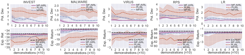
Figure 1: Results for numerical tasks. The line and shade are the median and variance over 10 independent runs, respectively.

6.2 Reward Recovery with Fixed Dynamics

The first experiment tests the capability of reward recovery with fixed environment dynamics. Results are depicted in Fig. 1. On all tasks, MF-AIRL achieves the closest performance to the expert with the same number of demonstrations and the fastest convergence with the number of demonstrations increases, suggesting that among all three algorithms, MF-AIRL is the most effective and efficient for imperfect demonstrations. MFIRL shows larger deviations even if the number of demonstrations is large. This may be owed to that MFIRL takes MFNE as the solution concept, thereby lacking the ability to tolerate suboptimal behaviours. PLIRL shows the largest deviation and variance. This is as expected because PLIRL is only suitable for socially optimal equilibria, while an ERMFNE is not socially optimal as it captures uncertainties in agent behaviours. Therefore, biased reward inferences occur when applying PLIRL to these tasks.

6.3 Policy Transfer across Varying Dynamics

The second experiment investigates the robustness against changing environment dynamics. We change the transition function (see Appendix D for details), recompute an ERMFNE $({\bm{\mu}}^{E}_{new},{\bm{\pi}}^{E}_{new})$ induced by the ground-truth reward function, compute the best-response policy ${\bm{\pi}}^{\omega}_{new}$ to ${\bm{\mu}}^{E}_{new}$ under the learned reward function (trained with 100 demonstrated trajectories), and calculate two metrics again. Results are summarised in Tab. 1. Consistently, MF-AIRL outperforms two baselines on all tasks. We attribute the high robustness of MF-AIRL to the following reasons: (1) MF-AIRL uses a potential function to mitigate the effect of reward shaping while two baselines do not; (2) The issue of biased inference in PLIRL can be exacerbated by the changing dynamics, as is argued in Chen et al. (2022). To summarise, MF-AIRL can recover ground-truth reward functions with high robustness to changing dynamics.

Task	Metric	Algorithm
		EXPERT	MF-AIRL	PLIRL	MFIRL
INVEST	Pol. Dev	–	0.24 (0.02)	1.06 (0.21)	0.78 (0.18)
	Exp. Ret	-35.87	-35.19 (0.51)	-37.73 (2.76)	-35.92 (0.98)
MALWARE	Pol. Dev	–	0.52 (0.01)	1.54 (1.20)	0.73 (0.14)
	Exp. Ret	-18.90	-18.49 (0.14)	-19.59 (0.29)	-18.82 (0.05)
VIRUS	Pol. Dev	–	1.48 (0.01)	1.76 (0.18)	1.55 (0.03)
	Exp. Ret	-1.24	-1.71 (0.02)	-2.66 (0.14)	-2.16 (0.06)
RPS	Pol. Dev	–	6.11 (0.46)	6.47 (0.98)	6.56 (0.82)
	Exp. Ret	93.16	93.36 (2.51)	91.99 (0.44)	91.28 (2.15)
LR	Pol. Dev	–	0.57 (0.04)	0.62 (0.22)	0.71 (0.07)
	Exp. Ret	-0.64	-1.70 (0.01)	-2.67 (1.01)	-1.93 (0.06)

Table 1: Results for new environment dynamics. Mean and variance are taken across 10 independent runs.

Task	Strength	Metric	Algorithm
			EXPERT	MF-AIRL	MFIRL
INVEST	$\beta=0$	Pol. Dev	–	0.45 (0.03)	0.44 (0.02)
		Exp. Ret	-35.05	-35.92 (0.68)	-35.54 (2.55)
	$\beta=0.1$	Pol. Dev	–	0.31 (0.02)	0.39 (0.04)
		Exp. Ret	-36.37	-37.08 (0.71)	-37.40 (1.08)
MALWARE	$\beta=0$	Pol. Dev	–	0.39 (0.07)	0.38 (0.07)
		Exp. Ret	-18.06	-19.15 (0.25)	-18.52 (0.51)
	$\beta=0.1$	Pol. Dev	–	0.41 (0.03)	0.50 (0.10)
		Exp. Ret	-19.36	-19.84 (0.22)	-20.39 (0.69)
VIRUS	$\beta=0$	Pol. Dev	–	1.50 (0.04)	1.34 (0.09)
		Exp. Ret	-1.17	-2.55 (0.04)	-1.61 (0.17)
	$\beta=0.1$	Pol. Dev	–	1.54 (0.01)	1.80 (0.07)
		Exp. Ret	-2.15	-2.61 (0.06)	-2.98 (0.43)
RPS	$\beta=0$	Pol. Dev	–	9.71 (0.24)	9.36 (0.40)
		Exp. Ret	94.27	93.21 (0.49)	93.58 (2.51)
	$\beta=0.1$	Pol. Dev	–	7.09 (0.54)	8.40 (0.40)
		Exp. Ret	91.43	90.43 (3.09)	89.40 (0.96)
LR	$\beta=0$	Pol. Dev	–	0.45 (0.07)	0.37 (0.08)
		Exp. Ret	-0.52	-2.60 (0.08)	-1.70 (1.08)
	$\beta=0.1$	Pol. Dev	–	0.68 (0.04)	0.70 (0.04)
		Exp. Ret	-0.64	-0.81 (0.04)	-0.96 (0.71)

Table 2: Comparisons between MF-AIRL and MFIRL on varying strength of entropy regularisation.

6.4 Weak Entropy Regularisation

If the entropy regularisation in ERMFNE is too strong, it becomes easy and trivial to perform MaxEnt IRL as the policy tends to select actions uniformly as a result of the maximum entropy principle. Our third experiment thus investigates the performance under weak entropy regularisation. Since PLIRL is known to lead to biased reward inference if the demonstrated equilibrium is not socially optimal, we eliminate it here and only compare two decentralised methods. To weaken the entropy regularisation, we set the coefficient $\beta$ in the expert ERMFNE to $0$ and $0.1$, respectively and sample 100 demonstrated trajectories from each. The environment dynamic is fixed. Results are summarised in Tab. 2. Note that an ERMFNE is recovered to an MFNE if $\beta=0$; this realises an experient complementary to the above two where all trajectories are sampled from an ERMFNE with $\beta=1$. It also enables a fair comparison between MF-AIRL and MFIRL as technically the they are designed under two prescribed equilibrium concepts.

With trajectories sampled from an MFNE ($\beta=0$), MF-AIRL shows a larger deviation from the expert compared to MFIRL, but on average its variance is lower. This fact can be attributed to the reason that a best-response policy in MFNE does not exist uniquely, though MFIRL is unbiased under MFNE. In contrast, MF-AIRL can always recover a unique best-response policy from a learned reward function, though with bias under MFNE. This result again validates our argument that by taking MFNE as the solution concept, MFIRL fails to elicit a unique policy from the learned reward function. While, even with a positive yet small strength of entropy regularisation ($\beta=0.1$), our MF-AIRL quickly outperforms MFIRL in terms of both accuracy and variance. This suggests that our MF-AIRL can handle imperfect behaviours, even with a small amount of uncertainties.

7 Concluding Remarks

In this paper, we propose MF-AIRL, the first probabilistic IRL framework effective for MFGs with imperfect demonstrations. We first extend MaxEnt IRL to MFGs based on a new solution concept termed ERMFNE, which allows us to characterise uncertainties in expert demonstrations using the maximum entropy principle. We then develop the practical MF-AIRL framework using an adversarial learning approach to solve a sampling-based approximation of MaxEnt IRL for MFGs. Experimental results on simulated tasks demonstrate the effectiveness and efficiency of MF-AIRL against existing IRL methods for MFGs.

We argue that MF-AIRL is worth following generalisations: (1) Continuous states and actions. The arguments in this paper still hold for continuous state-action spaces, except that some techniques (e.g., $\epsilon$-net (Guo et al., 2019)) are needed to discretise a mean field because it turns to a probability density function if states are continuous. (2) Infinite time horizon. When the time horizon tends to infinity, the mean field is shown to converge almost surely to a constant limit, resulting in the stationary MFNE (Subramanian and Mahajan, 2019). MF-AIRL is compatible with infinite time horizons because non-stationary equilibria recover stationary ones as special cases. (3) Generalised mean fields. Some work (Guo et al., 2019) generalises the mean field $\mu\in{{\mathcal{P}}}({{\mathcal{S}}})$ to $(\mu,\alpha)\in{{\mathcal{P}}}({{\mathcal{S}}}\times{{\mathcal{A}}})$ by additionally considering population’s average action $\alpha\in{{\mathcal{P}}}({{\mathcal{A}}})$. MF-AIRL is adaptive to generalised mean fields by incorporating the marginal distribution $\alpha$ in all mean field arguments. (4) Heterogeneous agents. A large-scale heterogeneous multi-agent system can be converted to a homogeneous system by considering the type of the agent as a component of states (Subramanian et al., 2020). Our MF-AIRL is therefore compatible with systems consisting of heterogeneous agents.

Appendices

A Proof of Theorem 3

Our proof of Theorem 3 relies on the following lemma from (Cui and Koeppl, 2021), which shows that an energy-based model can characterise the policy in ERMFNE in terms of action values.

Lemma A.1 ((Cui and Koeppl, 2021))

Let $({{\mathcal{S}}},{{\mathcal{A}}},P,\mu_{0},r)$ be an MFG with the entropy regularisation and $(\tilde{{\bm{\mu}}}^{\star},\tilde{{\bm{\pi}}}^{\star})$ be the ERMFNE. Denote the action value function (i.e., cumulative future rewards of selecting an action in a state) of $({\bm{\mu}},{\bm{\pi}})$ by

$$Q^{{\bm{\mu}},{\bm{\pi}}_{t+1:T-1}}(s_{t},a_{t},\mu_{t})\triangleq r(s_{t},a_{t},\mu_{t})+\\ \mathbb{E}_{{\bm{\pi}}_{t+1:T-1}}\left[\sum_{\ell=t+1}^{T-1}r(s_{\ell},a_{\ell},\mu_{\ell})+{{\mathcal{H}}}(\pi_{\ell}(\cdot|s_{\ell}))\right].$$

Then, the policy $\tilde{{\bm{\pi}}}^{\star}$ is in the form of

$$\tilde{\pi}^{\star}_{t}(a_{t}|s_{t})=\frac{e^{Q^{\tilde{{\bm{\mu}}}^{\star},\tilde{{\bm{\pi}}}_{t+1:T-1}}(s_{t},a_{t},\tilde{\mu}^{\star}_{t})}}{\sum_{a^{\prime}\in{{\mathcal{A}}}}e^{Q^{\tilde{{\bm{\mu}}}^{\star},\tilde{{\bm{\pi}}}_{t+1:T-1}}(s_{t},a^{\prime},\tilde{\mu}^{\star}_{t})}}.$$

A.1 Proof of Theorem 3

Proof 

Let $(\tilde{{\bm{\mu}}}^{\star},\tilde{{\bm{\pi}}}^{\star})$ be the ERMFNE for a MFG $({{\mathcal{S}}},{{\mathcal{A}}},p,\mu_{0},r)$. For an arbitrary policy ${\bm{\pi}}$, the probability of a trajectory $\tau=\{(s_{t},a_{t})\}_{t=0}^{T-1}$ induced by $({\bm{\mu}},{\bm{\pi}})$ satisfies the following distribution:

$$p_{1}(\tau)=\mu_{0}(s_{0})\cdot\prod_{t=0}^{T-1}P(s_{t+1}|s_{t},a_{t},\mu_{t})\cdot\prod_{t=0}^{T}\pi_{t}(a_{t}|s_{t}).$$ (A1)

Recall our desired energy-based trajectory distribution formula is

$$p_{2}(\tau)\propto\mu_{0}(s_{0})\cdot\prod_{t=0}^{T-1}P(s_{t+1}|s_{t},a_{t},\mu_{t})\cdot e^{R(\tau)}.$$

Let $D_{\mathrm{KL}}$ denote the Kullback-Leibler (KL) divergence. We now show that the ERMFNE $(\tilde{{\bm{\mu}}}^{\star},\tilde{{\bm{\pi}}}^{\star})$ is the optimal solution to the following optimisation problem:

$$\min_{{\bm{\mu}},{\bm{\pi}}}D_{\mathrm{KL}}\left(p_{1}(\tau)\parallel p_{2}(\tau)\right)\text{\em~{} s.t.~{} }{\bm{\mu}}=\Phi({\bm{\pi}}).$$ (A2)

The constraint enforces the condition of population consistency. Thus, fixing ${\bm{\mu}}$ as $\tilde{{\bm{\mu}}}^{\star}$, to show the ERMFNE $(\tilde{{\bm{\mu}}}^{\star},\tilde{{\bm{\pi}}}^{\star})$ is the optimal solution to Eq. (A2) is equivalent to show that $\tilde{{\bm{\pi}}}^{\star}$ is the optimal solution to the following optimisation problem:

$$\min_{{\bm{\pi}}}D_{\mathrm{KL}}\left(p_{1}(\tau)\parallel p_{2}(\tau)\right)\text{\em~{} where~{} }{\bm{\mu}}=\tilde{{\bm{\mu}}}^{\star}.$$ (A3)

Our proof is in a manner of dynamic programming. We construct the basic case for step $T-1$, where Eq. (A3) holds according to the definition of the policy in ERMFNE. Then, for each $t<T-1$, we construct the optimal policy for steps from $t$ to $T-1$ based on the optimal policy that is already constructed from $t+1$ to $T-1$. We show that the constructed optimal policy that minimises the above KL divergence is consistent with $\tilde{{\bm{\pi}}}^{\star}$ in ERMFNE. We next elaborate on the procedure of dynamic programming.

For simplicity, we omit the partition function for $p_{2}$ as it is a constant. Substituting $p_{1}(\tau)$ and $p_{2}(\tau)$ in Eq. (A3) with their definitions and roll out the KL-divergence, we obtain that maximising the KL-divergence between $p_{1}(\tau)$ and $p_{2}(\tau)$ is equivalent to the following optimisation problem

$$\max_{{\bm{\pi}}}\mathbb{E}_{\tau\sim p_{1}}\left[\log\frac{p_{2}(\tau)}{p_{1}(\tau)}\right]=\mathbb{E}_{\tau\sim p_{1}}\Bigg{[} \log\mu_{0}(s_{0})+\sum_{t=0}^{T-1}\left(r(s_{t},a_{t},\tilde{\mu}^{\star}_{t})+\log P(s_{t+1}|s_{t},a_{t},\tilde{\mu}^{\star}_{t})\right)-$$ (A4)

$$\log\mu_{0}(s_{0})-\sum_{t=0}^{T-1}\left(\log\pi_{t}(a_{t}|s_{t})+\log P(s_{t+1}|s_{t},a_{t},\tilde{\mu}^{\star}_{t})\right)\Bigg{]}$$

$$=\mathbb{E}_{\tau\sim p_{1}}\Bigg{[} \sum_{t=0}^{T-1}r(s_{t},a_{t},\tilde{\mu}^{\star}_{t})-\log\pi_{t}(a_{t}|s_{t})\Bigg{]}$$

We maximise the objective in Eq. (A4) using a dynamic programming method.

Consider the terminal step $t=T$, since the reward at the terminal step is always $0$, to maximise the entropy, the policy $\pi_{T}$ chooses actions evenly, i.e, $\tilde{\pi}^{\star}_{T}(a|s)=1/|{{\mathcal{A}}}|$ for any $a\in{{\mathcal{A}}}$ and $s\in{{\mathcal{S}}}$.

We then construct the base case that maximises $\pi_{T-1}$:

$$\max_{\pi_{T-1}}{} \mathbb{E}_{(s_{T-1},a_{T-1})\sim p_{1}}\left[r(s_{T-1},a_{T-1},\tilde{\mu}^{\star}_{T-1})-\log\pi_{T-1}(a_{T-1}|s_{T-1})\right]$$ (A5)

$$= \mathbb{E}_{(s_{T-1},a_{T-1})\sim p_{1}}\Bigg{[}-D_{\mathrm{KL}}\left(\pi_{T-1}(a_{T-1}|s_{T-1})\bigg{\|}\frac{e^{r(s_{T-1},a_{T-1},\tilde{\mu}^{\star}_{T-1})}}{e^{V(s_{T-1},\tilde{\mu}^{\star}_{T-1})}}\right)+V(s_{T-1},\tilde{\mu}^{\star}_{T-1})\Bigg{]},$$

where we define

$$V(s_{T-1},\tilde{\mu}^{\star}_{T-1})\triangleq\log\sum_{a^{\prime}\in{{\mathcal{A}}}}e^{r(s_{T-1},a^{\prime},\tilde{\mu}^{\star}_{T-1})}.$$

The optimal $\pi_{T-1}$ for Eq. (A5) is

$$\tilde{\pi}_{T-1}^{\star}(a_{T-1}|s_{T-1})=\frac{e^{r(s_{T-1},a_{T-1},\tilde{\mu}^{\star}_{T-1})}}{e^{V(s_{T-1},\tilde{\mu}^{\star}_{T-1})}}=\frac{e^{r(s_{T-1},a_{T-1},\tilde{\mu}^{\star}_{T-1})}}{\sum_{a^{\prime}\in{{\mathcal{A}}}}e^{r(s_{T-1},a^{\prime},\tilde{\mu}^{\star}_{T-1})}},$$ (A6)

which coincides with the form given in Lemma A.1.

With the optimal policy given in Eq. (A6), the KL-divergence in Eq. (A5) attains $0$ and Eq. (A5) attains the minimum $V(s_{T-1},\tilde{\mu}^{\star}_{T-1})$.

Then recursively, we can show that for any step $t<T-1$, $\pi_{t}$ is the maximiser of the following optimisation problem:

$$\max_{\pi_{t}}\mathbb{E}_{(s_{t},a_{t})\sim p_{1}}\left[-D_{\mathrm{KL}}\left(\pi_{t}(a_{t}|s_{t})\bigg{\|}\frac{e^{Q^{\tilde{{\bm{\mu}}}^{\star},\tilde{{\bm{\pi}}}^{\star}_{t+1:T-1}}(s_{t},a_{t},\tilde{\mu}_{t}^{\star})}}{e^{V^{\tilde{{\bm{\mu}}}^{\star},\tilde{{\bm{\pi}}}^{\star}_{t+1:T-1}}(s_{t},\tilde{\mu}_{t}^{\star})}}\right)+V^{\tilde{{\bm{\mu}}}^{\star},\tilde{{\bm{\pi}}}^{\star}_{t+1:T-1}}(s_{t},\tilde{\mu}_{t}^{\star})\right],$$ (A7)

where

$$V^{\tilde{{\bm{\mu}}}^{\star},\tilde{{\bm{\pi}}}^{\star}_{t+1:T-1}}(s_{t},\tilde{\mu}^{\star}_{t})\triangleq\log\sum_{a^{\prime}\in{{\mathcal{A}}}}e^{Q^{\tilde{{\bm{\mu}}}^{\star},\tilde{{\bm{\pi}}}^{\star}_{t+1:T-1}}(s_{t},a_{t},\tilde{\mu}^{\star}_{t})}.$$

In fact, $V^{{\bm{\mu}},{\bm{\pi}}_{t+1:T-1}}$ resembles the soft value function in soft Q-learning (Haarnoja et al., 2017).

The optimal policy for Eq. (A7) is given by

$$\pi_{t}(a_{t}|s_{t})=\frac{e^{Q^{\tilde{{\bm{\mu}}}^{\star},\tilde{{\bm{\pi}}}^{\star}_{t+1:T-1}}_{\mathrm{soft}}(s_{t},a_{t},\tilde{\mu}^{\star}_{t})}}{e^{V^{\tilde{{\bm{\mu}}}^{\star},\tilde{{\bm{\pi}}}^{\star}_{t+1:T-1}}_{\mathrm{soft}}(s_{t},\tilde{\mu}^{\star}_{t})}}=\frac{e^{Q^{\tilde{{\bm{\mu}}}^{\star},\tilde{{\bm{\pi}}}^{\star}_{t+1:T-1}}_{\mathrm{soft}}(s_{t},a_{t},\tilde{\mu}^{\star}_{t})}}{\sum_{a\in{{\mathcal{A}}}}e^{Q^{\tilde{{\bm{\mu}}}^{\star},\tilde{{\bm{\pi}}}^{\star}_{t+1:T-1}}_{\mathrm{soft}}(s_{t},a,\tilde{\mu}^{\star}_{t})}},$$

which coincides with the form given in Lemma A.1.  

B Proof of Theorem 4

Proof  The gradient of $\hat{L}$ concerning $\omega$ is given by:

$$\nabla_{\omega}\hat{L}\left(\omega;\hat{{\bm{\mu}}}^{E}\right) =\frac{1}{M}\sum_{j=1}^{M}\sum_{t=0}^{T-1}\nabla_{\omega}r_{\omega}\left(s_{j,t},a_{j,t},\hat{\mu}^{E}_{t}\right)-\nabla_{\omega}\log\hat{Z}_{\omega}$$ (B8)

$$=\frac{1}{M}\sum_{j=1}^{M}\sum_{t=0}^{T-1}\nabla_{\omega}r_{\omega}\left(s_{j,t},a_{j,t},\hat{\mu}^{E}_{t}\right)-\frac{1}{\hat{Z}_{\omega}}\nabla_{\omega}\hat{Z}_{\omega}$$

$$=\frac{1}{M}\sum_{j=1}^{M}\sum_{t=0}^{T-1}\nabla_{\omega}r_{\omega}\left(s_{j,t},a_{j,t},\hat{\mu}^{E}_{t}\right)-\sum_{j=1}^{M}\frac{e^{\sum_{t=0}^{T-1}r_{\omega}\left(s_{j,t},a_{j,t},\hat{\mu}^{E}_{t}\right)}}{\hat{Z}_{\omega}}\sum_{t=0}^{T-1}\nabla_{\omega}r_{\omega}\left(s_{j,t},a_{j,t},\hat{\mu}^{E}_{t}\right)$$

Let $\Pr\nolimits_{{{\mathcal{D}}}_{E}}(\tau)\triangleq\frac{1}{M}\sum_{j=1}^{M}\mathds{1}_{\{\tau_{j}=\tau\}}$ denote the empirical trajectory distribution, then Eq. (B8) is equivalent to

$$\nabla_{\omega}\hat{L}\left(\omega;\hat{{\bm{\mu}}}^{E}\right)= \sum_{j=1}^{M}\Pr\nolimits_{{{\mathcal{D}}}_{E}}(\tau_{j})\sum_{t=0}^{T-1}\nabla_{\omega}r_{\omega}\left(s_{j,t},a_{j,t},\hat{\mu}^{E}_{t}\right)$$ (B9)

$$-\sum_{j=1}^{M}\frac{e^{\sum_{t=0}^{T-1}r_{\omega}\left(s_{j,t},a_{j,t},\hat{\mu}^{E}_{t}\right)}}{\hat{Z}_{\omega}}\sum_{t=0}^{T-1}\nabla_{\omega}r_{\omega}\left(s_{j,t},a_{j,t},\hat{\mu}^{E}_{t}\right)$$

$$= \sum_{j=1}^{M}\left(\Pr\nolimits_{{{\mathcal{D}}}_{E}}(\tau_{j})-\frac{e^{\sum_{t=0}^{T-1}r_{\omega}\left(s_{j,t},a_{j,t},\hat{\mu}^{E}_{t}\right)}}{\hat{Z}_{\omega}}\right)\sum_{t=0}^{T-1}\nabla_{\omega}r_{\omega}\left(s_{j,t},a_{j,t},\hat{\mu}^{E}_{t}\right).$$

When the number of samples $M\to\infty$, $\Pr\nolimits_{{{\mathcal{D}}}_{E}}(\tau)$ tends to the true trajectory distribution $p(\tau)$ (see Eq. (5)) induced by ERMFNE. Meanwhile, according to the law of large numbers, $\hat{{\bm{\mu}}}\to{\bm{\mu}}^{E}$ with probability 1 as the number of samples $M\to\infty$. Let $\omega^{\star}$ be a maximiser of the likelihood objective in Eq. (7). Taking the limit as $M\to\infty$ and the optimality $\omega=\omega^{\star}$, we have:

$$\begin{aligned} \frac{e^{\sum_{t=0}^{T-1}r_{\omega^{\star}}\left(s_{j,t},a_{j,t},\mu^{E}_{t}\right)}}{\hat{Z}_{\omega^{\star}}}&=\frac{e^{\sum_{t=0}^{T-1}r_{\omega^{\star}}\left(s_{j,t},a_{j,t},\mu^{E}_{t}\right)}}{\sum_{j=1}^{M}e^{\sum_{t=0}^{T-1}r_{\omega^{\star}}\left(s_{j,t},a_{j,t},\mu^{E}_{t}\right)}}\\ &=\Pr(\tau_{j})\\ &=\Pr\nolimits_{{{\mathcal{D}}}_{E}}(\tau_{j})\end{aligned}.$$

Therefore, the gradient in Eq. (B9) will be zero; hence, the proof is complete.  

C Justifications for the Reward Shaping in MFGs

We show in the following theorem that for any potential function $g:{{\mathcal{S}}}\times{{\mathcal{P}}}({{\mathcal{S}}})\to\mathbb{R}$, the potential-based reward shaping can ensure the invariance of both ERMFNE and MFNE.

Theorem 5

Let any ${{\mathcal{S}}},{{\mathcal{A}}}$ be given. We say $F:{{\mathcal{S}}}\times{{\mathcal{A}}}\times{{\mathcal{P}}}({{\mathcal{S}}})\times{{\mathcal{S}}}\times{{\mathcal{P}}}({{\mathcal{S}}})\to\mathbb{R}$ is a potential-based reward shaping for MFG if there exists a real-valued function $g:{{\mathcal{S}}}\times{{\mathcal{P}}}({{\mathcal{S}}})\to\mathbb{R}$ such that $F(s_{t},a_{t},\mu_{t},s_{t+1},\mu_{t+1})=g(s_{t+1},\mu_{t+1})-g(s_{t},\mu_{t})$. Then, $F$ is sufficient and necessary to guarantee the invariance of the set of MFNE and ERMFNE in the sense that:

• Sufficiency: Every MFNE or ERMFNE in the MFG ${{\mathcal{M}}}^{\prime}=({{\mathcal{S}}},{{\mathcal{A}}},P,\mu_{0},r+F)$ is also a MFNE or ERMFNE in ${{\mathcal{M}}}=({{\mathcal{S}}},{{\mathcal{A}}},P,\mu_{0},r)$;

• Necessity: If $F$ is not a potential-based reward shaping, then there exist an initial mean field $\mu_{0}$, transition function $P$, horizon $T$, and reward function $r$ such that no MFNE or ERMFNE in ${{\mathcal{M}}}^{\prime}$ is an equilibrium in ${{\mathcal{M}}}$.

Proof  We first prove the sufficiency. First, we show the set of MFNE remains invariant under the potential-based reward shaping $F$. Let ${\bm{\mu}}$ be an arbitrary MF flow. The optimal action function for the MFG induced by ${\bm{\mu}}$, denoted by $Q^{\star}$, fulfil the Bellman equation:

$$Q^{\star}(s_{t},a_{t})=r(s_{t},a_{t},\mu_{t})+\mathbb{E}_{s_{t+1}\sim p}\left[\max_{a_{t+1}\in{{\mathcal{A}}}}Q^{\star}(s_{t+1},a_{t+1})\right].$$

Applying some simple algebraic manipulation gives:

$$~{}~{}~{}~{}~{}Q^{\star}(s_{t},a_{t})-g(s_{t},\mu_{t})$$

$$=r(s_{t},a_{t},\mu_{t})-g(s_{t},\mu_{t})+g(s_{t+1},\mu_{t+1})+\mathbb{E}_{s_{t+1}\sim P}\left[\max_{a_{t+1}\in{{\mathcal{A}}}}(Q^{\star}(s_{t+1},a_{t+1})-g(s_{t+1},\mu_{t+1}))\right]$$

$$=r(s_{t},a_{t},\mu_{t})+F(s_{t},a_{t},\mu_{t},s_{t+1},\mu_{t+1})+\mathbb{E}_{s_{t+1}\sim P}\left[\max_{a_{t+1}\in{{\mathcal{A}}}}(Q^{\star}(s_{t+1},a_{t+1})-g(s_{t+1},\mu_{t+1}))\right].$$

From here, we know that the above equation is exactly the Bellman equation induced by ${\bm{\mu}}$ with the reward function $r+F$, and $Q^{\star}(s_{t},a_{t})-g(s_{t},\mu_{t})$ is the unique set of optimal Q values. Since $\operatorname*{arg\,max}_{a\in{{\mathcal{A}}}}Q^{\star}(s_{t},a_{t})-g(s_{t},\mu_{t})=\operatorname*{arg\,max}_{a\in{{\mathcal{A}}}}Q^{\star}(s_{t},a_{t})$, we have that for any fix a MF flow, any optimal policy of ${{\mathcal{M}}}^{\prime}$ is also an optimal policy of ${{\mathcal{M}}}$. Hence, we finish the proof of the sufficiency of MFNE.

Next, we will show the sufficiency of ERMFNE. We write $\tilde{Q}^{\star}$ for the optimal action-value functions for the MFG with the entropy regularisation such that

$$\tilde{Q}^{\star}(s_{t},a_{t})=r(s_{t},a_{t},\mu_{t})+\mathbb{E}_{s_{t+1}\sim p}\left[\sum_{a_{t+1}\in{{\mathcal{A}}}}\frac{e^{\tilde{Q}^{\star}(s_{t+1},a_{t+1})}}{\sum_{a^{\prime}\in{{\mathcal{A}}}}e^{\tilde{Q}^{\star}(s_{t},a^{\prime})}}\tilde{Q}^{\star}(s_{t+1},a_{t+1})\right].$$

Using the same manner as we show the invariance of MFNE, we have:

$$~{}~{}~{}~{}~{}\tilde{Q}^{\star}(s_{t},a_{t})-g(s_{t},\mu_{t})$$

$$=r(s_{t},a_{t},\mu_{t})-g(s_{t},\mu_{t})+g(s_{t+1},\mu_{t+1})$$

$$~{}~{}~{}~{}~{}+\mathbb{E}_{s_{t+1}\sim P}\left[\frac{e^{\tilde{Q}^{\star}(s_{t+1},a_{t+1})-g(s_{t+1},\mu_{t+1})}}{\sum_{a^{\prime}\in{{\mathcal{A}}}}e^{\tilde{Q}^{\star}(s_{t},a^{\prime})-g(s_{t+1},\mu_{t+1})}}(\tilde{Q}^{\star}(s_{t+1},a_{t+1})-g(s_{t+1},\mu_{t+1}))\right]$$

$$=r(s_{t},a_{t},\mu_{t})-g(s_{t},\mu_{t})+g(s_{t+1},\mu_{t+1})$$

$$~{}~{}~{}~{}~{}+\mathbb{E}_{s_{t+1}\sim P}\left[\frac{e^{\tilde{Q}^{\star}(s_{t+1},a_{t+1})}}{\sum_{a^{\prime}\in{{\mathcal{A}}}}e^{\tilde{Q}^{\star}(s_{t},a^{\prime})}}(\tilde{Q}^{\star}(s_{t+1},a_{t+1})-g(s_{t+1},\mu_{t+1}))\right].$$

Hence, we know that $\tilde{Q}^{\star}(s_{t},a_{t})-g(s_{t},\mu_{t})$ is the set of optimal action values induced by ${\bm{\mu}}$ under the reward function $r+F$. Thus, any optimal policy of ${{\mathcal{M}}}^{\prime}$ is also an optimal policy of ${{\mathcal{M}}}$. Hence, we finish the proof of sufficiency for MFNE.

We next show the necessity by constructing a counter-example where a non-potential-based reward shaping can change the set of MFNE and ERMFNE. Consider the Left-Right problem (Cui and Koeppl, 2021), which is also used as a task in experiments. At each step, each agent is at a position (state) of either “left”, “right” or “center”, and can choose to move either “left” or “right”, receives a reward according the current population density (mean field) at each position, and with probability one (dynamics) reaches “left” or “right”. Once an agent leaves the “centre”, she can never head back and can only be in either left or right thereafter. Formally, we configure the MFG as follows: ${{\mathcal{S}}}=\{C,L,R\}$, ${{\mathcal{A}}}={{\mathcal{S}}}\setminus\{C\}$, initial mean field $\mu_{0}(C)=1$ (i.e., all agents are at “center” initially) and the reward function

$$r(s,a,\mu_{t})=-\mathds{1}_{\{s=L\}}\cdot\mu_{t}(L)-\mathds{1}_{\{s=R\}}\cdot\mu_{t}(R).$$

This reward setting means that each agent will incur a negative reward determined by the population density at her current position. The transition function is deterministic that directs an agent to the next state with probability one:

$$P(s_{t+1}|s_{t},a_{t},\mu_{t})=\mathds{1}_{\{s_{t+1}=a_{t}\}}.$$

This configuration is illustrated below.

Now, we consider the case that the time horizon $=1$.

Since all agents are at “center” initially, we have that $\mu_{1}^{\star}(L)=\pi_{0}^{\star}(L|C)$ and $\mu_{1}^{\star}(R)=\pi_{0}^{\star}(R|C)$. Therefore, we have that the expected return of each agent under MFNE is

$$~{}-1\cdot\pi_{0}^{\star}(L|C)\cdot\mu_{1}^{\star}(L)-1\cdot\pi_{0}^{\star}(R|C)\cdot\mu_{1}^{\star}(R)$$

$$= ~{}-(\pi_{0}^{\star}(L|C))^{2}-(1-\pi_{0}^{\star}(L|C))^{2}$$

$$= ~{}-\left(2(\pi_{0}^{\star}(L|C))^{2}-2\pi_{0}^{\star}(L|C)+1\right).$$

Clearly, the expected return attains the maximum when $\pi_{0}^{\star}(L|C)=1/2$. Therefore, any MFNE $({\bm{\mu}}^{\star},{\bm{\pi}}^{\star})$ under the configuration above must fulfil $\pi^{\star}_{0}(R|C)=\pi^{\star}_{0}(L|C)=1/2$ and $\pi^{\star}_{1}$ can be arbitrary. And clearly, there exists a unique ERMFNE $(\tilde{{\bm{\mu}}}^{\star},\tilde{{\bm{\pi}}}^{\star})$ such that any action at any state and any time step is chosen with probability $1/2$. This result is also shown as a case study in (Cui and Koeppl, 2021).

Next, we change the reward function by adding an additional reward based on actions to the original reward function. We penalise the action “left” by a negative value $-1$, i.e.,

$$r^{\prime}(s,a,\mu_{t})=r(s,a,\mu_{t})-\mathds{1}_{\{a=L\}}=-\mathds{1}_{\{s=L\}}\cdot\mu_{t}(L)-\mathds{1}_{\{s=R\}}\cdot\mu_{t}(R)-\mathds{1}_{\{a=L\}}.$$

This equivalent to that an action-based reward shaping function $F(s_{t},a_{t},\mu_{t},s_{t+1},\mu_{t+1})=g(s_{t+1},a_{t+1},\mu_{t+1})-g(s_{t},a_{t},\mu_{t})$ is added to the original reward function where

$$g(s_{t},a_{t},\mu_{t})=-\mathds{1}_{\{a_{t}=L\}}.$$

The following diagram shows this new reward configuration.

Now, let us investigate the form of MFNE and ERMFNE under this new reward configuration. We first show the set of MFNE induced by the new reward function is no longer the same as that induced by the original reward function. Consider the step $t=1$ (the last step), since the reward of moving right is always higher than moving left by 1 and MFNE aims to maximise cumulative rewards, all agent will move right, i.e., $\pi_{1}^{\star}(R|L)=\pi_{1}^{\star}(R|R)=1$. Hence, each agent earns a reward $-\mu_{1}^{\star}(L)$ if she is at “left” and $-\mu_{1}^{\star}(R)$ otherwise. Using the fact that $\mu_{1}^{\star}(L)=\pi_{0}^{\star}(L|C)$ and $\mu_{1}^{\star}(R)=\pi_{0}^{\star}(R|C)$, we have that the expected return of each agent under MFNE is

$$~{}-1\cdot\pi_{0}^{\star}(L|C)+0\cdot\pi_{0}^{\star}(R|C)-\mu_{1}^{\star}(L)\cdot\pi_{0}^{\star}(L|C)-\mu_{1}^{\star}(R)\cdot\pi_{0}^{\star}(R|C)$$

$$= ~{}-\pi_{0}^{\star}(L|C)-(\pi_{0}^{\star}(L|C))^{2}-(\pi_{0}^{\star}(R|C))^{2}$$

$$= ~{}-\pi_{0}^{\star}(L|C)-(\pi_{0}^{\star}(L|C))^{2}-(1-\pi_{0}^{\star}(L|C))^{2}$$

$$= ~{}-\left(2(\pi_{0}^{\star}(L|C))^{2}-\pi_{0}^{\star}(L|C)+1\right).$$

From here, we have that the expected return attains the maximum when $\pi_{0}^{\star}(L|C)=1/4$, contradicting the MFNE induced by the original reward function.

Next, we show that the ERMFNE induced by the new reward function also changes. Again, consider the last step. According to the definition of ERMFNE, we have

$$\tilde{\pi}^{\star}_{1}(L|L)=\frac{e^{-\tilde{\mu}_{1}^{\star}(L)}}{e^{-\tilde{\mu}_{1}^{\star}(L)}+e^{-\tilde{\mu}_{1}^{\star}(L)-1}}.$$

Therefore, $\tilde{\pi}^{\star}_{1}(L|L)=1/2$ if and only if $\tilde{\mu}_{1}^{\star}(L)=\tilde{\mu}_{1}^{\star}(L)+1$. A contradiction occurs.  

D Descriptions for Numerical Tasks

The detailed descriptions below are adapted from (Chen et al., 2022).

D.1 Investment in Product Quality

Model. This model is adapted from (Weintraub et al., 2010) and (Subramanian and Mahajan, 2019) that captures the investment decisions in a fragmented market with a large number of firms. Each firm produces the same kind of product. The state of a firm $s\in{{\mathcal{S}}}=\{0,1,\ldots,9\}$ denotes the product quality. At each step, each firm decides whether or not to invest in improving the quality of the product. Thus the action space is ${{\mathcal{A}}}=\{0,1\}$. When a firm decides to invest, its product quality increases uniformly at random from its current value to the maximum value 9 if the average quality in the market for that product is below a particular threshold $q$. If this average quality value is above $q$, then the product quality gets only half of the improvement compared to the former case. This implies that when the average quality in the economy is below $q$, it is easier for each firm to improve its quality. When a firm does not invest, its product quality remains unchanged. Formally, the dynamics is given by:

$$s_{t+1}=\left\{\begin{aligned} &s_{t}+\lfloor\chi_{t}(10-s_{t})\rfloor,\text{~{}~{}if~{}~{}}\langle\mu_{t}\rangle<q\text{~{}~{}and~{}~{}}a_{t}=1\\ &s_{t}+\lfloor\chi_{t}(10-s_{t})/2\rfloor,\text{~{}~{}if~{}~{}}\langle\mu_{t}\rangle\geq q\text{~{}~{}and~{}~{}}a_{t}=1\\ &s_{t},\text{~{}~{}if~{}~{}}a_{t}=0\end{aligned}\right..$$

An agent incurs a cost due to its investment and earns a positive reward due to its own product quality and a negative reward due to the average product quality, which we denote by

$$\langle\mu_{t}\rangle\triangleq\sum_{s\in{{\mathcal{S}}}}s\cdot\mu_{t}(s).$$ (D10)

The final reward is given as:

$$r(s_{t},a_{t},\mu_{t})=d\cdot s_{t}/10-c\cdot\langle\mu_{t}\rangle-\alpha\cdot a_{t}$$

D.1.1 Settings.

We set $d=0.3$, $c=0.2$, $\alpha=0.2$ and probability density $f$ for $\chi_{t}$ as $U(0,1)$. We set the threshold $q$ to $4$ and $5$, respectively. The initial mean field $\mu_{0}$ is set as a uniform distribution, i.e, $\mu_{0}(s)=1/|{{\mathcal{S}}}|$ for all $s\in{{\mathcal{S}}}$.

D.2 Malware Spread

D.2.1 Model.

The malware spread model is presented in (Huang and Ma, 2016, 2017) and used as a simulated study for MFG in (Subramanian and Mahajan, 2019). This model is representative of several problems with positive externalities, such as flu vaccination and economic models involving the entry and exit of firms. Here, we present a discrete version of this problem: Let ${{\mathcal{S}}}=\{0,1,\ldots,9\}$ denote the state space (level of infection), where $s=0$ is the most healthy state and $s=9$ is the least healthy state. The action space ${{\mathcal{A}}}=\{0,1\}$, where $a=0$ means $\mathtt{DoNothing}$ and $a=1$ means $\mathtt{Intervene}$. The dynamics is given by

$$s_{t+1}=\left\{\begin{aligned} &s_{t}+\lfloor\chi_{t}(10-s_{t})\rfloor,\text{~{}~{}if~{}~{}}a_{t}=0\\ &0,\text{~{}~{}if~{}~{}}a_{t}=1\end{aligned}\right.,$$

where $\{\chi_{t}\}_{0\leq t\leq T}$ is a $[0,1]$-valued i.i.d. process with probability density $f$. The above dynamics means the $\mathtt{DoNothing}$ action makes the state deteriorate to a worse condition, while the $\mathtt{Intervene}$ action resets the state to the most healthy level. Rewards are coupled through the average health level of the population, i.e., $\langle\mu_{t}\rangle$ as defined in Eq.(D10). An agent incurs a cost $(k+\langle\mu_{t}\rangle)s_{t}$, which captures the risk of getting infected, and an additional cost of $\alpha$ for performing the $\mathtt{Intervene}$ action. The reward sums over all negative costs:

$$r(s_{t},a_{t},\mu_{t})=-(k+\langle\mu_{t}\rangle)s_{t}/10-\alpha\cdot a_{t}.$$

D.2.2 Settings.

Following (Subramanian and Mahajan, 2019), we set $k=0.2$, $\alpha=0.5$, and the probability density $f$ to the uniform distribution $U(0,1)$ for the original dynamics. The initial mean field $\mu_{0}$ is set as a uniform distribution.

D.3 Virus Infection

D.3.1 Model.

This is a virus infection used as a case study in (Cui and Koeppl, 2021). There is a large number of agents in a building. Each can choose between “social distancing” ($D$) or “going out” ($U$). If a “susceptible” ($S$) agent chooses social distancing, they may not become “infected” ($I$). Otherwise, an agent may become infected with a probability proportional to the number of infected agents. If infected, an agent will recover with a fixed chance every time step. Both social distancing and being infected have an associated negative reward. Formally, let ${{\mathcal{S}}}=\{S,I\},{{\mathcal{A}}}=\{U,D\},r(s,a,\mu_{t})=-\mathds{1}_{\{s=I\}}-0.5\cdot\mathds{1}_{\{s=D\}}$. The transition probability is given by

$$P(s_{t+1}=S|s_{t}=I,\cdot,\cdot) =0.3$$

$$P(s_{t+1}=I|s_{t}=S,a_{t}=U,\mu_{t}) =0.9^{2}\cdot\mu_{t}(I)$$

$$P(s_{t+1}=I|s_{t}=S,a_{t}=D,\cdot) =0.$$

D.3.2 Settings.

The initial mean field $\mu_{0}$ is set as a uniform distribution.

D.4 Rock-Paper-Scissors

This model is adapted by (Cui and Koeppl, 2021) from the generalized non-zero-sum version of Rock-Paper-Scissors game (Shapley, 1964). Each agent can choose between “rock” ($R$), “paper” ($P$) and “scissors” ($S$), and obtains a reward proportional to double the number of beaten agents minus the number of agents beating the agent. Formally, let ${{\mathcal{S}}}={{\mathcal{A}}}=\{R,P,S\}$, and for any $a\in{{\mathcal{A}}},\mu_{t}\in{{\mathcal{P}}}({{\mathcal{S}}})$:

$$r(R,a,\mu_{t}) =2\cdot\mu_{t}(S)-1\cdot\mu_{t}(P),$$

$$r(P,a,\mu_{t}) =4\cdot\mu_{t}(R)-2\cdot\mu_{t}(S),$$

$$r(S,a,\mu_{t}) =6\cdot\mu_{t}(P)-3\cdot\mu_{t}(R).$$

The transition function is deterministic: $p(s_{t+1}|s_{t},a_{t},\mu_{t})=\mathds{1}_{\{s_{t+1}=a_{t}\}}.$

D.4.1 Settings.

The initial mean field $\mu_{0}$ is set as a uniform distribution.

D.5 Left-Right

D.5.1 Model.

This model is used in (Cui and Koeppl, 2021). A group of agents makes sequential decisions to move “left” or “right”. At each step, each agent is at a position (state) either “left”, “right” or “center”, and can choose to move either “left” or “right”, receives a reward according the current population density (mean field) at each position, and with probability one (dynamics) they reach “left” or “right”. Once an agent leaves “centre”, she can never head back and can only be on the left or right thereafter. Formally, we configure the MFG as follows: ${{\mathcal{S}}}=\{C,L,R\}$, ${{\mathcal{A}}}={{\mathcal{S}}}\setminus\{C\}$, the reward

$$r(s,a,\mu_{t})=-\mathds{1}_{\{s=L\}}\cdot\mu_{t}(L)-\mathds{1}_{\{s=R\}}\cdot\mu_{t}(R).$$

This reward setting means each agent will incur a negative reward determined by the population density at her current position. The transition function is deterministic that directs an agent to the next state with probability one: $P(s_{t+1}|s_{t},a_{t},\mu_{t})=\mathds{1}_{\{s_{t+1}=a_{t}\}}.$

D.5.2 Settings.

The initial mean field $\mu_{0}$ is set as $\mu_{0}(L)=\mu_{0}(R)=0.5$.

E Implementation Details

The experimental settings below are adapted from (Chen et al., 2022).

E.0.1 Feature representations.

We use one-hot encoding to represent states and actions. Let $\{1,2,\ldots,|{{\mathcal{S}}}|\}$ denote an enumeration of ${{\mathcal{S}}}$ and $\left[s_{[1]},s_{[2]},\ldots,s_{[|{{\mathcal{S}}}|]}\right]$ denote a vector of length $|{{\mathcal{S}}}|$, where each component stands for a state in ${{\mathcal{S}}}$. The state $j$ is denoted by $\big{[}0,\ldots,0,s_{[j]}=1,0,$ $\ldots,0\big{]}$. An action is represented in the same manner. A mean field $\mu$ is represented by a vector $\left[\mu(s_{[1]}),\mu(s_{[2]}),\ldots,\mu(s_{[|{{\mathcal{S}}}|]})\right]$, where $\mu(s_{[i]})$ denotes the proportion of agents that are in the $i$th state.

E.0.2 Reward Models.

The reward mode $r_{\omega}$ takes as input the concatenation of feature vectors of $s$, $a$ and $\mu$ and outputs a scalar as the reward. We adopt the neural network (a four-layer perceptron) with the Adam optimiser and the Leaky ReLU activation function. The sizes of the two hidden layers are both 64. The learning rate is $10^{-4}$.

E.0.3 Computation of ERMFNE.

In ERMFNE expert training, we repeat the fixed point iteration to compute the MF flow. We terminate at the $i$th iteration if the mean squared error over all steps and all state is below or equal to $10^{-10}$, i.e.,

$$\frac{1}{(T-1)|{{\mathcal{S}}}|}\sum_{t=1}^{T-1}\sum_{s\in{{\mathcal{S}}}}\left(\mu^{(i)}_{t}(s)-\mu^{(i-1)}_{t}(s)\right)^{2}\leq 10^{-10}.$$

References

- Anahtarci et al. (2020) Berkay Anahtarci, Can Deha Kariksiz, and Naci Saldi. Q-learning in regularized mean-field games. arXiv preprint arXiv:2003.12151, 2020.
- Carmona et al. (2013) René Carmona, François Delarue, and Aimé Lachapelle. Control of mckean–vlasov dynamics versus mean field games. Mathematics and Financial Economics, 7(2):131–166, 2013.
- Chen et al. (2022) Yang Chen, Libo Zhang, Jiamou Liu, and Shuyue Hu. Individual-level inverse reinforcement learning for mean field games. In Proceedings of the 21st International Conference on Autonomous Agents and Multi-agent Systems, 2022.
- Cui and Koeppl (2021) Kai Cui and Heinz Koeppl. Approximately solving mean field games via entropy-regularized deep reinforcement learning. In International Conference on Artificial Intelligence and Statistics, pages 1909–1917. PMLR, 2021.
- Devlin and Kudenko (2011) Sam Devlin and Daniel Kudenko. Theoretical considerations of potential-based reward shaping for multi-agent systems. In The 10th International Conference on Autonomous Agents and Multiagent Systems, pages 225–232. ACM, 2011.
- Elie et al. (2020) Romuald Elie, Julien Pérolat, Mathieu Laurière, Matthieu Geist, and Olivier Pietquin. On the convergence of model free learning in mean field games. In Thirty-Fourth AAAI Conference on Artificial Intelligence, pages 7143–7150, 2020.
- Finn et al. (2016) Chelsea Finn, Sergey Levine, and Pieter Abbeel. Guided cost learning: deep inverse optimal control via policy optimization. In Proceedings of the 33rd International Conference on International Conference on Machine Learning, pages 49–58, 2016.
- Fu et al. (2018) Justin Fu, Katie Luo, and Sergey Levine. Learning robust rewards with adverserial inverse reinforcement learning. In International Conference on Learning Representations, 2018.
- Gabaix (2014) Xavier Gabaix. A sparsity-based model of bounded rationality. The Quarterly Journal of Economics, 129(4):1661–1710, 2014.
- Goodfellow et al. (2014) Ian Goodfellow, Jean Pouget-Abadie, Mehdi Mirza, Bing Xu, David Warde-Farley, Sherjil Ozair, Aaron Courville, and Yoshua Bengio. Generative adversarial nets. Advances in neural information processing systems, 27, 2014.
- Guo et al. (2019) Xin Guo, Anran Hu, Renyuan Xu, and Junzi Zhang. Learning mean-field games. In Advances in Neural Information Processing Systems, pages 4967–4977, 2019.
- Guo et al. (2020) Xin Guo, Renyuan Xu, and Thaleia Zariphopoulou. Entropy regularization for mean field games with learning. arXiv preprint arXiv:2010.00145, 2020.
- Haarnoja et al. (2017) Tuomas Haarnoja, Haoran Tang, Pieter Abbeel, and Sergey Levine. Reinforcement learning with deep energy-based policies. In International Conference on Machine Learning, pages 1352–1361. PMLR, 2017.
- Harstad and Selten (2013) Ronald M Harstad and Reinhard Selten. Bounded-rationality models: tasks to become intellectually competitive. Journal of Economic Literature, 51(2):496–511, 2013.
- Huang and Ma (2016) Minyi Huang and Yan Ma. Mean field stochastic games: Monotone costs and threshold policies. In 2016 IEEE 55th Conference on Decision and Control (CDC), pages 7105–7110. IEEE, 2016.
- Huang and Ma (2017) Minyi Huang and Yan Ma. Mean field stochastic games with binary actions: Stationary threshold policies. In 2017 IEEE 56th Annual Conference on Decision and Control (CDC), pages 27–32. IEEE, 2017.
- Huang et al. (2006) Minyi Huang, Roland P Malhamé, Peter E Caines, et al. Large population stochastic dynamic games: closed-loop mckean-vlasov systems and the nash certainty equivalence principle. Communications in Information & Systems, 6(3):221–252, 2006.
- Lasry and Lions (2007) Jean-Michel Lasry and Pierre-Louis Lions. Mean field games. Japanese Journal of Mathematics, 2(1):229–260, 2007.
- Lee et al. (2021) Kiyeob Lee, Desik Rengarajan, Dileep Kalathil, and Srinivas Shakkottai. Reinforcement learning for mean field games with strategic complementarities. In International Conference on Artificial Intelligence and Statistics, pages 2458–2466. PMLR, 2021.
- Ng and Russell (2000) Andrew Y Ng and Stuart J Russell. Algorithms for inverse reinforcement learning. In Proceedings of the Seventeenth International Conference on Machine Learning, pages 663–670, 2000.
- Ng et al. (1999) Andrew Y Ng, Daishi Harada, and Stuart Russell. Policy invariance under reward transformations: Theory and application to reward shaping. In ICML, volume 99, pages 278–287, 1999.
- Ortega and Braun (2011) Daniel Alexander Ortega and Pedro Alejandro Braun. Information, utility and bounded rationality. In International Conference on Artificial General Intelligence, pages 269–274. Springer, 2011.
- Ratliff et al. (2006) Nathan D Ratliff, J Andrew Bagnell, and Martin A Zinkevich. Maximum margin planning. In Proceedings of the 23rd International Conference on Machine Learning, pages 729–736, 2006.
- Shapley (1964) Lloyd Shapley. Some topics in two-person games. Advances in game theory, 52:1–29, 1964.
- Song et al. (2018) Jiaming Song, Hongyu Ren, Dorsa Sadigh, and Stefano Ermon. Multi-agent generative adversarial imitation learning. In Advances in Neural Information Processing Systems, pages 7461–7472, 2018.
- Subramanian and Mahajan (2019) Jayakumar Subramanian and Aditya Mahajan. Reinforcement learning in stationary mean-field games. In Proceedings of the 18th International Conference on Autonomous Agents and Multi-agent Systems, pages 251–259, 2019.
- Subramanian et al. (2020) Sriram Subramanian, Pascal Poupart, Matthew E Taylor, and Nidhi Hegde. Multi type mean field reinforcement learning. In Proceedings of the 19th International Conference on Autonomous Agents and Multi-agent Systems, pages 411–419, 2020.
- Weintraub et al. (2010) Gabriel Y Weintraub, C Lanier Benkard, and Benjamin Van Roy. Computational methods for oblivious equilibrium. Operations research, 58(4-part-2):1247–1265, 2010.
- Yang et al. (2018a) Jiachen Yang, Xiaojing Ye, Rakshit Trivedi, Huan Xu, and Hongyuan Zha. Learning deep mean field games for modeling large population behavior. In International Conference on Learning Representations, 2018a.
- Yang et al. (2018b) Y Yang, R Luo, M Li, M Zhou, W Zhang, and J Wang. Mean field multi-agent reinforcement learning. In 35th International Conference on Machine Learning, volume 80, pages 5571–5580. PMLR, 2018b.
- Yu et al. (2019a) Lantao Yu, Jiaming Song, and Stefano Ermon. Multi-agent adversarial inverse reinforcement learning. In International Conference on Machine Learning, pages 7194–7201, 2019a.
- Yu et al. (2019b) Lantao Yu, Tianhe Yu, Chelsea Finn, and Stefano Ermon. Meta-inverse reinforcement learning with probabilistic context variables. Advances in Neural Information Processing Systems, 32, 2019b.
- Ziebart et al. (2008) Brian D Ziebart, Andrew Maas, J Andrew Bagnell, and Anind K Dey. Maximum entropy inverse reinforcement learning. In Proceedings of the 23rd AAAI Conference on Artificial Intelligence, pages 1433–1438, 2008.
- Ziebart et al. (2010) Brian D Ziebart, J Andrew Bagnell, and Anind K Dey. Modeling interaction via the principle of maximum causal entropy. In Proceedings of the 27th International Conference on Machine Learning, pages 1255–1262, 2010.