Borel Edge Colorings for Finite Dimensional Groups

Abstract

We study the potential of Borel asymptotic dimension, a tool introduced recently in [2], to help produce Borel edge colorings of Schreier graphs generated by Borel group actions. We find that it allows us to recover the classical bound of Vizing in certain cases, and also use it to exactly determine the Borel edge chromatic number for free actions of abelian groups.

1 Introduction

In a recent paper [2], Conley et al. introduced a new tool, Borel asymptotic dimension, to the study of Borel combinatorics. We will define this notion in Section 2, but for now we emphasize that they exhibited several useful consequences which follow when a locally finite Borel graph has finite Borel asymptotic dimension, including hyperfiniteness for its connectedness relation, and Borel vertex colorings using relatively few colors.

The aim of this paper is to add to this list by showing applications of finite Borel asymptotic dimension to edge colorings.

Let $X$ be a standard Borel space and $G\subset X\times X$ a Borel graph on $X$. An edge coloring of $G$ is a function $c:G\rightarrow Y$ which sends adjacent edges in $G$, that is, edges sharing a vertex, to distinct elements of $Y$, or “colors”. Such a $c$ is called a $k$-coloring if $|Y|=k$. The edge chromatic number of $G$, denoted $\chi^{\prime}(G)$, is the smallest cardinal $k$ such that $G$ admits a $k$-coloring. The Borel edge-chromatic number of $G$, denoted $\chi_{B}^{\prime}(G)$, is the smallest cardinal $k$ such that $G$ admits a Borel $k$-coloring. See [8] for a survey of these and related notions.

The Borel graphs of interest to us in this paper will be those generated by Borel actions of finitely generated groups. A marked group is a pair $(\Gamma,S)$ where $\Gamma$ is a group and $S$ is a finite symmetric generating set for $\Gamma$ not containing 1. We will sometimes omit the $S$ if it will not cause confusion. Let $X$ be a standard Borel space and $a:\Gamma\curvearrowright X$ a free Borel action. Let $G(a,S)$ denote the Schreier graph generated by this action. This is the graph defined by setting $x,y\in X$ adjacent if and only if $\gamma\cdot_{a}x=y$ for some $\gamma\in S$.

Note that all the notions in the above paragraph make sense even if $S$ does not generate the entire group $\Gamma$. We shall sometimes use them in this case.

A classical theorem of Vizing states that if $G$ is a graph with maximum degree $d$, then $\chi^{\prime}(G)\leq d+1$. Of natural interest is the extent to which this bound continues to hold in the Borel setting. Grebík and Pikhurko have shown that this bound holds in the measurable setting when $G$ is measure preserving [5], but on the other hand Marks has shown that it fails in the general Borel setting, even for acyclic $G$ [10].

As was previously promised, in section 2 we shall see a precise definition of Borel asymptotic dimension for graphs and Borel actions. Actually, of more direct use to use will be a variant of this number, also from [2], called Borel asymptotic separation index. Our main result in Section 3 will be that the Vizing’s bound holds in the Borel context for graphs generated by certain group actions when this index is 1.

Theorem 1.

Let $a:\Gamma\curvearrowright X$ be a free Borel action of a marked group $(\Gamma,S)$ on a standard Borel space $X$ with Borel asymptotic separation index 1, and such that none of the elements of $S$ have odd order. Then $\chi_{B}^{\prime}(G(a,S))\leq|S|+1$.

We emphasize that the condition on the generators in Theorem 1 implies that $\chi^{\prime}(G(a,S))=|S|$. Nevertheless, we will see in Section 4 that the “$+1$” in Theorem 1 cannot always be removed.

In [2], it is shown that finite Borel asymptotic dimension implies a Borel asymptotic separation index of 1. Several quite general classes of groups, including those with a polynomial growth rate, are also shown to always have finite Borel asymptotic dimension for their free Borel actions. The work of that paper therefore provides us with many groups to which Theorem 1 can be applied.

We will also see in Section 3 that Theorem 1 can be applied to finite extensions of marked groups which satisfy its constraints.

Finally, we will note in Section 3 that Theorem 1 implies that the Vizing bound holds in certain Baire measurable or measurable settings.

It follows from the third most recent paragraph that free actions of abelian groups always have finite Borel asymptotic dimension, although this was known earlier from work of Gao et al. [4]. In Section 4, we will see how a more specific analysis allows us to improve on Theorem 1 for these groups by exactly determining their edge chromatic numbers.

Theorem 2.

Let $(\Gamma,S)$ be a marked group with $\Gamma=\Delta\times\mathbb{Z}^{d}$ abelian, where $\Delta$ is the torsion part of $\Gamma$ and $d\in\omega$ is its free rank. Let $a:\Gamma\curvearrowright X$ be the action of $\Gamma$ on its Bernoulli shift, and $G=G(a,S)$

1. If $d=0$, $\chi^{\prime}(G)=\chi_{B}^{\prime}(G)=|S|$ if and only if $\Delta$ has even order. (and $\chi^{\prime}(G)=\chi^{\prime}(G)=|S|+1$ otherwise.)

2. If $d=1$, $\chi^{\prime}(G)=|S|$, and $\chi_{B}^{\prime}(G)=|S|$ if and only if $\Delta$ has even order (and $\chi_{B}^{\prime}(G)=|S|+1$ otherwise.)

3. If $d\geq 2$, $\chi^{\prime}(G)=\chi_{B}^{\prime}(G)=|S|$.

The point of using the Bernoulli shift in the above statement is that arbitrary Borel free actions of $\Gamma$ always admit Borel $\Gamma$-equivariant embeddings to the Bernoulli shift [7], and so the chromatic numbers for the Bernoulli shift are the supremums of the chromatic numbers of arbitrary free actions of $\Gamma$.

Note that the statements in parentheses follow from Vizing’s Theorem/ Theorem 1 (or rather the aforementioned generalization of the theorem to finite extensions) and the fact that when $\Gamma$ is finite, its discrete and Borel combinatorics coincide.

During the preparation of this project, we became aware that this result was recently arrived at two other times independently in the special case $\Gamma=\mathbb{Z}^{d}$ and $S=$ the standard generating set. [6],[1] (the latter for $d=2$). The key ideas from the proof given in [6] appear also in this work, but some additional ideas are needed to extend the result to arbitrary abelian groups and arbitrary generating sets. Additionally, we learned via personal communication that the authors of [6] were aware of Theorem 1. Our paper provides the first write up of this result.

2 Borel asymptotic dimension and asymptotic separation index

In this section we will review the relevant definitions and facts from [2] regarding Borel asymptotic dimension and asymptotic separation index.

We start with the discrete versions of these notions: Let $G$ be a locally finite graph on a set $X$, and $N$ a positive integer. Let $G^{\leq N}$ denote the distance $N$-graph of $G$. This is the graph which sets two vertices adjacent if and only if there is a path from one to the other of length at most $N$.

The asymptotic separation index of $G$, denoted $\textnormal{asi}(G)$ is the infimum over $s\in\omega$ such that the following holds: For every positive integer $N$, $X$ can be partitioned into $s+1$ sets, say $U_{0},\ldots,U_{s}$, such that for each $i$, the induced graph $G^{\leq N}\upharpoonright U_{i}$ has only finite connected components. The asymptotic dimension of $G$, denoted $\textnormal{asdim}(G)$, is defined similarly, except now the connected components of each $G^{\leq N}\upharpoonright U_{i}$ are required to have a uniform (finite) bound on their size.

Let $G$ now be a Borel graph on a standard Borel space $X$. The Borel asymptotic separation index and Borel asymptotic dimension of $G$, denoted $\textnormal{asi}_{B}(G)$ and $\textnormal{asdim}_{B}(G)$ respectively, are defined exactly as their discrete counterparts were, except that now all the $U_{i}$’s are required to be Borel sets.

Now let $\Gamma$ be a finitely generated group, and $a:\Gamma\curvearrowright X$ a free Borel action. It is easy to verify that none of the above numbers for the graph $G(a,S)$ depend on the choice $S$ of generating set for $\Gamma$. We can thus talk about the (Borel) asymptotic separation index and (Borel) asymptotic dimension of the action $a$ itself.

We now list some facts. If $G$ has only finite connected components, then $\textnormal{asi}_{B}(G)$ is trivially 0 and its Borel and discrete combinatorics coincide, so until Section 4 assume this is not the case. The following facts, which were referenced in Section 1, can be used to establish that Borel actions of free abelian groups have Borel asymptotic separation index 1, and are also relevant to the discussion more broadly.

Theorem 3 ([2]).

Let $\Gamma$ be a finitely generated group with polynomial growth rate for its Cayley graph(s). Then any free Borel action of $\Gamma$ has finite Borel asymptotic dimension.

Theorem 4 ([2]).

Let $G$ be a locally finite Borel graph with $\textnormal{asdim}_{B}(G)<\infty$. Then $\textnormal{asi}_{B}(G)=1$

These next facts will sometimes allow us to recover Vizing’s bound in the Baire measurable and measurable contexts, even for groups for which $\textnormal{asi}_{B}\neq 1$.

Theorem 5 ([3],[2]).

Let $G$ be a locally finite Borel graph on a Polish space $X$. Then there is a Borel $G$-invariant comeager set $X^{\prime}\subset X$ such that $\textnormal{asi}_{B}(G\upharpoonright X^{\prime})=1$.

Theorem 6 ([3]).

Let $G$ be a locally finite Borel graph on a standard Borel probability measure space $(X,\mu)$ such that the connectedness equivalence relation of $G$ is hyperfinite. Then there is a Borel $G$-invariant $\mu$-conull set $X^{\prime}\subset X$ such that $\textnormal{asi}_{B}(G\upharpoonright X^{\prime})=1$.

3 Degree plus one colorings

In this section we prove Theorem 1 and give some examples where it cannot be improved.

3.1 Proof of Theorem 1

Let $G$ be a graph on a set $X$. An injective $G$-ray is an injective infinite sequence $x_{0},x_{1},\ldots\in X$ such that $(x_{i},x_{i+1})\in G$ for all $i\in\omega$. Given a set $U\subset X$ and an $n\in\omega$, let us write $B(U,n)$ for the ball of radius $n$ around $U$. That is, the set of all points $x\in X$ whose path distance to $U$ is less than or equal to $n$. For $m\in\omega$, let us write $A(U,n,m)=B(U,m)-B(U,n)$. One can check that if $G$ and $U$ are Borel, these sets are always Borel.

The following two lemmas together explain how having a Borel asymptotic separation index of 1 will help us to construct edge colorings.

Lemma 1.

Suppose $G$ is a locally finite graph Borel graph on a space $X$ with $\textnormal{asi}_{B}(G)=1$, and $d\in\omega$. Then we can find pairwise disjoint Borel sets $V_{1},\ldots,V_{d}\subset X$ such that any injective $G$-ray contains infinitely many edges within each $V_{i}$.

Proof.

Since the tail of an injective $G$-ray is still an injective $G$-ray, it suffices to prove this with “infinitely many edges” replaced by “an edge”.

Let $X=U_{0}\sqcup U_{1}$ be a Borel partition of $X$ witnessing $\textnormal{asi}_{B}(G)=1$ for $N=4d+1$. That is, such that the graphs $G^{\leq N}\upharpoonright U_{0}$ and $G^{\leq N}\upharpoonright U_{1}$ both have only finite connected components. Set $V_{i}=A(U_{0},2(i-1),2i)$ for each $1\leq i\leq d$. Also set $W=X\setminus B(U_{0},2d)$. As was mentioned above, these are all still Borel. Let us now show these $V_{i}$’s work.

Let $x=(x_{n})$ be an injective $G$-ray. We first show that $x$ contains some point from $W$. Suppose not. Then for each $n$, there is a $y_{n}\in U_{0}$ whose path distance to $x_{n}$ is less than or equal to $2d$. Now for each $n$, going from $y_{n}$ to $x_{n}$, then to $x_{n+1}$, then to $y_{n+1}$, produces a path from $y_{n}$ to $y_{n+1}$ of length at most $2d+1+2d=N$, so all the $y_{n}$’s are in the same $G^{\leq N}\upharpoonright U_{0}$-connected component. By definition of $U_{0}$, then, the set $\{y_{n}\mid n\in\omega\}$ is finite. But now $x$ gives infinitely many points within distance $2d$ of this set, contradicting local finiteness.

Similarly, $x$ must contain some point from $U_{0}$. Let $x_{n}\in W$ and $x_{m}\in U_{0}$. We can assume $m<n$. Now the path distance from $x_{i}$ to $U_{0}$ changes by at most 1 each time $i$ is incremented by 1. Thus, since $x_{m}$ has distance 0 from $U_{0}$ and $x_{n}$ has distance greater than $2d$ from $U_{0}$, for each $1\leq i\leq d$, there must be some $m<j<n$ such that $x_{j}$ and $x_{j+1}$ have distance $2i-1$ and $2i$ respectively from $U_{0}$. Then $(x_{j},x_{j+1})$ is an edge of $x$ contained in $V_{i}$, as desired.

∎

Lemma 2.

Let $a:\mathbb{Z}\rightarrow X$ be a free Borel action of $\mathbb{Z}$, and $S$ the usual generating set for $\mathbb{Z}$. Suppose $V\subset X$ is a Borel set with the property that every injective $G(a,S)$-ray contains infinitely many edges within $V$. Then there is a Borel 3-edge coloring of $G(a,S)$, say with the colors $1,2$, and $3$, such that the color 3 only occurs on edges contained within $V$.

Proof.

A well known theorem from [9] (Proposition 4.2) states that for locally finite Borel graphs, it is always possible to find Borel maximal independent sets. Apply this to the edge graph of $G(a,S)\upharpoonright V$ to get a maximal set of edges $A$ contained within $V$ such that no two edges in $A$ share a vertex. Give all the edges in $A$ the color 3.

By maximality and the defining condition for the set $V$, these edges occur infinitely often in both directions along each $\mathbb{Z}$-orbit. Thus, the connected components of $G(a,S)\setminus A$ are all simply finite paths. These can of course be 2-colored with the colors 1 and 2, and since they are all finite, this can be done in a Borel fashion. (For example, by fixing a Borel linear order on the space of 2-edge colored finite subgraphs of $G(a,S)$, and picking the least 2-coloring in this order for each path above.) ∎

The proof of Theorem 1 is now easy:

Proof.

By hypothesis, we may write $S=S_{0}\sqcup S_{1}$, where $S_{0}$ contains all of our generators of infinite order, and $S_{1}$ contains all of our elements of even (finite) order. For each $\gamma\in S_{1}$, the connected components of the graph $G(a,\{\gamma^{\pm 1}\})$ are all even (finite) cycles, or just single edges if $\gamma$ has order 2. Thus they may be 2-colored in a Borel fashion as in the previous proof (or just 1-colored if $\gamma$ has order 2). Thus we may Borel $|S_{1}|$-color the edges in $G(a,S_{1})$.

It now suffices to Borel $|S_{0}|+1$-color the edges in $G(a,S_{0})$ using a disjoint set of colors. Let $S_{0}=\{\gamma_{1}^{\pm 1},\ldots,\gamma_{d}^{\pm 1}\}$, so that $|S_{0}|=2d$. We will use the color set $\{1,\ldots,2d+1\}$. Let $V_{1},\ldots,V_{d}\subset X$ be the sets from Lemma 1. Since $\langle\gamma_{i}\rangle\cong\mathbb{Z}$ for each $i$, by Lemma 2 we may for each $i$ color the edges in $G(a,\{\gamma_{i}^{\pm 1}\})$ using the colors $2i-1$, $2i$, and $2d+1$ such that the color $2d+1$ only appears on edges contained within $V_{i}$. Since the $V_{i}$’s are pairwise disjoint, this does not cause any color conflicts, so we are done. ∎

We now wish to see that we can extend Theorem 1 to finite extensions. To do this, it will be helpful to slightly expand our notion of graph to allow for multiple edges.

Let $\Gamma$ be a group and $S\subset\Gamma$ a finite symmetric multi-set of generators for it not containing 1. That is, the elements of $S$ can appear with some multiplicity. With $a:\Gamma\curvearrowright X$ a Borel free action as before, let $G(a,S)$ denote the Borel-multigraph where now points $x$ and $y$ are connected with one edge for each $\gamma\in S$ such that $\gamma\cdot x=y$. Edge colorings can be defined as before. Of course, if $x$ and $y$ have multiple edges between them, those all need different colors in an edge coloring.

Observe that Theorem 1 still holds, with the same proof, if $S$ is allowed to be a multi-set. This allows us to prove:

Corollary 1.

Let $a:\Gamma\curvearrowright X$ be a free Borel action of a marked group $(\Gamma,S)$ on a standard Borel space $X$ with Borel asymptotic separation index 1. Suppose $\Delta\leq\Gamma$ is a finite normal subgroup of $\Gamma$, and that for each $\gamma\in S\setminus\Delta$, the image of $\gamma$ in the quotient $\Gamma/\Delta$ does not have odd order. Then $\chi_{B}^{\prime}(G(a,S))\leq|S|+1$.

Proof.

Write $S=S_{0}\sqcup S_{1}$, where $S_{1}=S\cap\Delta$. Consider first the graph $G(a,S_{1})$. Its connected components are all contained within $\Delta$-orbits, and therefore finite. They are also $|S_{1}|$-regular, so by the classical Vizing’s Theorem and the argument from the final paragraph of Lemma 2, we may find a Borel $(|S_{1}|+1)$-edge coloring of this graph, say using the color set $C$.

Now let $\overline{X}$ be the Borel space of $\Delta$-orbits. Then $a$ induces a free Borel action, say $\overline{a}$, of $\Gamma/\Delta$ on $\overline{X}$. Let $\overline{S_{0}}$ be the multi-set which results from considering the images of the elements of $S_{0}$ in $\Gamma/\Delta$. By the last paragraph before the statement of the corollary, we may find a Borel $(|S_{0}|+1)$-edge coloring using a disjoint set of colors from $C$, say $C^{\prime}$, of $G(\overline{a},\overline{S_{0}})$. Now, given an edge $(x,\gamma\cdot x)$ in $G(a,S_{0})$, give it the color received by the edge $(\Delta\cdot x,\Delta\gamma\cdot x)$ in $G(\overline{a},\overline{S_{0}})$ corresponding to $\gamma$. This results in a Borel $(|S_{0}|+1)$-edge coloring of $G(a,S_{0})$ since whenever $x,y$ are distinct vertices in the same $\Delta$-orbit, the edges $(x,\gamma\cdot x)$ and $(y,\gamma\cdot y)$ are disjoint.

Amalgamating these two colorings gives us a Borel $(|S|+2)$-edge coloring of $G(a,S)$, but we can remove a color: Fix a color $c$ from $C$. For each $\Delta$-orbit, say $E\in\overline{X}$, $E$ has degree $|S_{0}|$ in the graph $G(\overline{a},\overline{S_{0}})$, and therefore is incident to only $|S_{0}|$ colors in our coloring of that graph. By our construction, it is still incident to only those colors in resulting coloring of $G(a,S_{0})$. Thus, we may pick a color $c^{\prime}$ from $C^{\prime}$ which $E$ does not meet. Then we may may change the color of any edge within $E$ colored $c$ to $c^{\prime}$. This process maintains Borel-ness, and results in an edge coloring not using $c$, hence a $|S|+1$-edge coloring. ∎

The following variant of Collary 1 will be used in Section 4:

Corollary 2.

Using the notation from the proof of Corollary 1,  suppose $\chi^{\prime}(G(a,S_{1}))=|S_{1}|$ (That is, the Cayley graph of $(\Delta,S_{1})$ is degree-edge colorable) and $S_{1}\neq\emptyset$. Then $\chi_{B}^{\prime}(G(a,S))=|S|$.

Proof.

Repeat the proof of Corollary 1, but now where the color set $C$ has size $|S_{1}|$. The condition $S_{1}\neq\emptyset$ is needed for the final step in the proof where we fix a color from $C$. ∎

Corollary 1 also generalizes a previous result of this author, which was proved using similar ideas [13]:

Corollary 3.

Let $a:\Gamma\curvearrowright X$ be a free Borel action of a marked group $(\Gamma,S)$ with two ends. Then $\chi_{B}^{\prime}(G(a,S))\leq|S|+1$.

Proof.

Two ended groups are always finite extensions of $\mathbb{Z}$ or the infinite dihedral group $D_{\infty}$, neither of which have any odd order elements. Furthermore a Borel asymptotic separation index of 1 is automatic by Theorem 3 since $\Gamma$ has linear growth rate, though this also follows from earlier work of Miller [11]. ∎

Similarly, Corollary 1 implies Vizing’s bound for any action of an abelian group:

Corollary 4.

Let $a:\Gamma\curvearrowright X$ be a free Borel action of an abelian marked group $(\Gamma,S)$. Then $\chi_{B}^{\prime}(G(a,S))\leq|S|+1$.

Proof.

By the fundamental theorem of finitely generated abelian groups, $\Gamma$ is a finite extension of some $\mathbb{Z}^{d}$. This implies it has polynomial (degree $d$) growth rate, and $\mathbb{Z}^{d}$ does not have any odd order elements. ∎

Note that the combination of Corollary 3 and Theorem 2 actually render this Corollary redundant. It is still nice to state here, though, as Theorem 2 will require somewhat more work.

We now pause briefly to address the measurable and Baire measurable situations. If $G$ is a Borel graph on a polish space $X$, we denote by $\chi_{BM}^{\prime}(G)$ the minimum of $\chi_{B}^{\prime}(G\upharpoonright X^{\prime})$ as $X^{\prime}$ ranges over all Borel comeager $G$-invariant subsets of $X$. If $X$ is instead equipped with a Borel probability measure $\mu$, $\chi_{\mu}^{\prime}(G)$ is defined similarly. Note that these numbers are both lower bounds for $\chi_{B}^{\prime}(G)$. Now, Theorems 5 and 6 have the following obvious consequences:

Corollary 5.

If we replace $\chi_{B}^{\prime}$ with $\chi_{BM}^{\prime}$, Theorem 1 and Corollary 1 hold for Borel actions on Polish spaces without any assumptions on asymptotic separation index.

Similarly in the measurable setting for actions with hyperfinite orbit equivalence relation.

3.2 Examples of tightness

Let us now consider when the “$+1$” in Theorem 1 can’t be removed. It is well known that there are free Borel actions of $\mathbb{Z}$ with its usual generating set which cannot be even Baire measurably 2-edge colored [9] (page 11, essentially), and so the bound in Theorem 1 is certainly sometimes tight. It would be reasonable, however, to chalk this up to the fact that 2-colorings are very rigid. For example, the following fact shows that the situation can sometimes be very different for graphs of max degree $>2$:

Theorem 7 ([8]).

If $G$ is an acyclic, $d$-regular Borel graph on a polish space and $d>2$, then $\chi_{BM}^{\prime}(G)=d$.

Thus it is natural to ask for examples in our situation for larger degrees. The following shows that that Theorem 1 remains tight for graphs of arbitrarily large degree, even if they are also assumed to be bipartite. It also provides one of the directions in the $d=1$ case of Theorem 2.

Proposition 1.

Let $(\Gamma,S)$ be a marked group with $\Gamma=\Delta\times\mathbb{Z}$ and $\Delta$ finite of odd order. Let $a:\Gamma\curvearrowright X$ be the usual action of $\Gamma$ on its Bernoulli shift. Then $G(a,S)$ does not admit a Baire measurable perfect matching (i.e, it does not admit a Borel perfect matching on a $\Gamma$-invariant comeager set). In particular $\chi_{BM}^{\prime}(G(a,S))=\chi_{B}^{\prime}(G(a,S))=|S|+1$.

Proof.

Suppose, to the contrary, there is a Borel $\Gamma$-invariant comeager set $X^{\prime}\subset X$ and a Borel perfect matching $M\subset(G(a,S)\upharpoonright X)$.

Start by defining $\overline{a}:\mathbb{Z}=\Gamma/\Delta\curvearrowright\overline{X}$, $S_{0}$, and $\overline{S_{0}}$ exactly as in the proof of Corollary 1. Also let $\overline{X^{\prime}}\subset\overline{X}$ be the set of $\Delta$-orbits contained in $X^{\prime}$.

Let $\overline{M}\subset G(\overline{a},\overline{S_{0}})$ be the sub-multigraph which includes an edge between distinct $\Delta$ orbits $y$ and $y^{\prime}$ for each edge between $y$ and $y^{\prime}$ in $M$. Since $\Delta$ has odd order, each orbit $y\in\overline{X^{\prime}}$ must be contained in an odd number of edges in $\overline{M}$.

Let $n\in\omega$ large enough so that $S\subset\Delta\times(-n,n)$. For any edge $(y,m\cdot y)\in G(\overline{a},\overline{S_{0}})$ with $m>0$, define $y$ to be the left endpoint of that edge and $m\cdot y$ to be the right endpoint. For $y\in\overline{X^{\prime}}$, define $F(y)$ to be the number of edges in $\overline{M}$ with a right endpoint in $[0,n]\cdot y$ and a left endpoint not in $[0,n]\cdot y$. Put another way, this is the number of edges in $\overline{M}$ which leave the set $[0,n]\cdot y$ to the left.

Let us compare $F(y)$ and $F(1\cdot y)$. For an edge of $\overline{M}$ to be counted in $F(1\cdot y)$ but not $F(y)$, it would have to either have $y$ has a left endpoint, or $(n+1)\cdot y$ as a right endpoint. Since $\overline{S_{0}}\subset(-n,n)$, though, no edge with $(n+1)\cdot y$ as a right endpoint can leave the set $[1,n+1]\cdot y$ to the left, and so this cannot occur. Thus our edge would have to have the form $(y,m\cdot y)$ for some $0<m<n$, and conversely any edge with this form is counted in $F(1\cdot y)$ but not $F(y)$.

Similarly, for an edge of $\overline{M}$ to be counted in $F(y)$ but not $F(1\cdot y)$, it would have to have $y$ as its right endpoint or $(n+1)\cdot y$ as its left endpoint. The latter is absurd, though, and so our edge would have to have the form $(m\cdot y,y)$ for some $m<0$. Once again, conversely any edge with this form is counted in $F(y)$ but not $F(1\cdot y)$.

Now, $y$ must be the left or right endpoint of each edge in $\overline{M}$ which it belongs to. Let $L$, and $R$ be the number of such edges falling into these respective cases. By the above discussing, we can conclude $F(1\cdot y)=F(y)+L-R$. By an earlier comment, though, $L+R$ is odd, so $F(1\cdot y)=F(y)+1$ (mod 2). Thus, if we define $f(y)$ to be the mod 2 value of $F(y)$, $f$ is a 2-vertex coloring of $G(\overline{a},\{\pm 1\})\upharpoonright\overline{X^{\prime}}$. It is also clearly Borel since $M$ was. This is well known to be impossible for nonmeager $X^{\prime}$ by a basic ergodicity argument [9] (page 11), so we are done.

Finally, the conclusions about the edge chromatic numbers follow from this and Corollary 3, since an $|S|$-edge coloring is a decomposition into perfect matchings.

∎

Note that this fails if we do not use the convention that $S$ must be finite. Indeed it is not hard to construct Borel perfect matchings for the Borel graph on $X$ above which connects any two points in the same $\Gamma$-orbit.

3.3 Open problems

We end this section by listing interesting open problems related to Theorem 1.

First, for Schreier graphs, it seems to be open whether any of the assumptions of the theorem are necessary:

Problem 1.

Is there any marked group $(\Gamma,S)$ and free Borel action $a:\Gamma\upharpoonright X$ such that $\chi_{B}^{\prime}(G(a,S))>|S|+1$?

Natural candidates to resolve this question are the free groups with their usual generating sets. It follows from the results in [10] that the Schreier graphs of these marked groups do not necessarily admit Borel pefect matchings, ruling out Borel degree-edge colorings, but not much else seems to be known. (See Problem 5.37 in [8].)

It is also unclear whether the presence of a group action is necessary:

Problem 2.

Let $G$ be a locally finite $d$-regular Borel graph with $\textnormal{asi}_{B}(G)=1$. Is $\chi_{B}^{\prime}(G)\leq d+1$?

It may be necessary to add an assumption of bipartite-ness to get an affirmative answer to this problem as a replacement to Theorem 1’s prohibition of odd-order generators. This restricted version of the problem still seems to be open. Note that by Theorem 5, an affirmative answer to Problem 2 would imply that Vizing’s theorem holds in complete generality in the Baire measurable setting.

Given Theorem 1, one way to make progress on Problem 2 in the case where $d$ is even would be to find so-called Schreier decorations of $G$ which are Borel. These are orientations of the edges of $G$ along with edge colorings so that each vertex ends up with exactly one in and one out edge of each color, and so they essentially realize $G$ as the Schreier graph of some not-necessarily free group action. Some recent progress has been made in this area: See [12], [1]. Even more generally, it would be useful to simply find Borel ways of decomposing $G$ into graphs of max degree $2$.

Finally, given Proposition 1 it is interesting to ask whether any groups other than finite extensions of $\mathbb{Z}$ can provide examples where the degree plus one bound is tight.

Problem 3.

Is there a marked group $(\Gamma,S)$ and a free Borel action $a:\Gamma\curvearrowright X$ satisfying the hypothesis of Theorem 1 for which $\chi_{B}^{\prime}(G(a,S))=|S|+1$, and for which $\Gamma$ is not a finite extension of $\mathbb{Z}$?

See Question 38 in [1] for a similar problem. Note that by Theorem 2, the answer is “No” for abelian $\Gamma$.

4 Degree colorings for abelian groups

In this section we prove Theorem 2. In two situations the theorem asserts the non-existence of degree colorings: In the discrete setting when $d=0$ and $\Delta$ has odd order, and in the Borel setting when $d=1$ and $\Delta$ has odd order. We have already mentioned that the latter is covered by Proposition 1. The former is obvious since a finite graph with an odd number of vertices cannot admit a perfect matching. Therefore in this section we can focus on constructing degree colorings in the remaining cases.

Throughout, let $a$,$X$,$\Gamma$,$S$, $d$, and $\Delta$ be as in the statement of the theorem, unless otherwise stated. Note, though, that nothing in this section is specific to the Bernoulli shift. We only use that $a$ is a free Borel action of $\Gamma$.

4.1 Free rank 0

In this subsection we complete the proof of statement 1 of Theorem 2 by showing that if $\Gamma=\Delta$ is an even order finite abelian group, then $\chi^{\prime}(G(a,S))=|S|$. Note that this will imply the same for $\chi_{B}^{\prime}(G(a,S))$, by the argument from the second half of Lemma 2. While it seems unlikely that this result is original, our coverage of it will introduce a general technique which will be useful for dealing with the torsion part when $d>0$. We feel it is also simply nice to include for the sake of completeness.

It suffices to consider the case when $a$ is the action of $\Delta$ on itself by multiplication. In this case our graph is called the Cayley graph of $(\Delta,S)$.

The following lemma is not specific to the case $d=0$.

Lemma 3.

Let $\Delta^{\prime}\leq\Gamma$ be a finite proper subgroup. Let $\overline{\Gamma}=\Gamma/\Delta^{\prime}$, and then define $\overline{a}:\overline{\Gamma}\curvearrowright\overline{X}$, $S_{0}$, and $\overline{S_{0}}$ as in the proof of Corollary 1. If $\chi^{\prime}(G(\overline{a},\overline{S_{0}}))=|{S_{0}}|$, then $\chi^{\prime}(G(a,S))=|S|$. Likewise for the Borel edge chromatic numbers of these graphs.

Proof.

Let $S_{1}=S\cap\Delta^{\prime}=S\setminus S_{0}$. By hypothesis, we may find a $|S_{0}|$-edge coloring of $\chi_{B}^{\prime}(G(\overline{a},\overline{S_{0}}))$, say using the set of colors $C$. As in the proof of Corollary 1, we may lift this to a $|S_{0}|$-edge coloring of $G(a,S_{0})$ by giving the edge $(x,\gamma\cdot x)$ for $x\in X$ and $\gamma\in S_{0}$ whichever color was given to the edge $(\Delta^{\prime}\cdot x,\gamma\Delta^{\prime}\cdot x)$ in $G(\overline{a},\overline{S_{0}})$ corresponding to $\gamma$.

Fix a color $c\in C$, which exists since $\Delta^{\prime}$ is proper, so $S_{0}$ is nonempty. Consider the subgraph $G^{\prime}$ of $G(a,S)$ consisting of $G(a,S_{1})$ along with all the edges colored $c$ in the previous step.

Since, in our coloring of $G(\overline{a},\overline{S_{0}})$, the set of edges colored $c$ gives a perfect matching, each connected component of our subgraph looks like the following: Two adjacent $\Delta$-orbits, say $y$ and $\gamma\cdot y$ for some $\gamma\in S_{0}$, with all the internal edges from $S_{1}$, along with all edges between them of the form $(x,\gamma\cdot x)$ for $x\in y$.

Fix a set $C^{\prime}$ of $|S_{1}|+1$ colors disjoint from $C$. We now use $C^{\prime}$ to edge color the above component. First, by Vizing’s theorem, we may use $C^{\prime}$ to color the edges within $y$. Now, for every such edge, say $(x,x^{\prime})$, give the edge $(\gamma\cdot x,\gamma\cdot x^{\prime})$ the same color. Since $\Gamma$ is abelian, this colors all edges within $\gamma\cdot y$ without conflict. Finally, for each $x\in y$, by this construction the set of colors of edges in $y$ meeting $x$ is the same as the set of colors of edges in $\gamma\cdot y$ meeting $\gamma\cdot x$. This set has size $|S_{1}|$, though, so we still have one free color, and can assign it to the edge $(x,\gamma\cdot x)$, completing our coloring.

Thus we can edge color $G^{\prime}$ using $C^{\prime}$, and we already have an edge coloring of $G(a,S)\setminus G^{\prime}$ using $C\setminus\{c\}$, so unioning these gives a coloring using $|C|^{\prime}+|C|-1=|S_{1}|+1+|S_{0}|-1=|S|$ colors as desired.

Finally, if our original coloring was Borel, our lift will still be Borel, and then our construction can be done in a Borel fashion since we only need to work with finite components. Again this uses the argument from Lemma 2. ∎

Statement 1 now follows:

Proof.

Since $\Delta$ has even order, we may by the fundemental theorem of finite abelian groups find an index 2 subgroup $\Delta^{\prime}\leq\Delta$. We now wish to apply Lemma 3 with this choice of $\Delta^{\prime}$. We clearly can, though, since we will have $\overline{\Gamma}=\mathbb{Z}/2$, and so $G(\overline{a},\overline{S_{0}})$ will just consist of two points with $|S_{0}|$-many edges between them. ∎

4.2 Free rank $\geq 2$

In this subsection we complete the proof of Statement 3 of Theorem 2. Applying Lemma 3 with $\Delta^{\prime}=\Delta$, we reduce to the case $\Gamma=\mathbb{Z}^{d}$, but where we now allow multiplicity for the generators in $S$. For the rest of the subsection, assume $(\Gamma,S)$ has this form.

For motivation, consider Figures 1 and 2. The former shows that we can think about the proof of Theorem 1 as follows: For each $i$, the orbits of $\gamma_{i}$ are edge colored using mostly the colors $2i-1$ and $2i$, but with an occasional $2d+1$ thrown in to help align parity.

The latter makes an analogy between this and our upcomming proof of Statement 3. For notational convenience, consider the case where $S=\{\pm e_{i}\mid 1\leq i\leq d\}$ is the standard generating set, where $e_{i}=(0,\ldots,0,1,0,\ldots,0)$, with the $1$ in the $i$-th coordinate. We will still color the orbits of each $e_{i}$ using mostly the colors $2i-1$ and $2i$, but as before we will need to occasionally break parity. Thanks to the structure of $\mathbb{Z}^{d}$, though, when $d\geq 2$ we will be able to do this by “borrowing” a color from some $e_{j}$-edge, $j\neq i$.

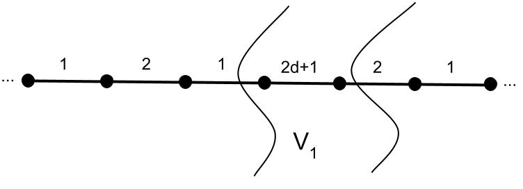
Figure 1: The key idea in the proof of Theorem 1

. The color $2d+1$ is used (within the region $V_{1}$) to “break parity” along the orbits of $\gamma_{1}$.

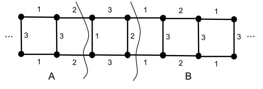
Figure 2: The key idea in the proof of Theorem 2. Now parity along the horizontal orbits is broken without the use of an additional color. The regions $A$ and $B$ are labeled so that they can be referenced later.

4.2.1 Borrowing colors

We will now describe a general setup for using this “borrowing” idea. See Figure 3 for a visualization. Let $\gamma_{1},\gamma_{2}\in S$ such that $\langle\gamma_{1},\gamma_{2}\rangle\cong\mathbb{Z}^{2}$. That is, $\gamma_{1}$ and $\gamma_{2}$ are not scalar multiples of eachother. Work in some finite subset $U$ of some $\mathbb{Z}^{d}$-orbit, with two disjoint subsets $A,B\subset U$. Let $S^{\prime}=\{\pm\gamma_{1},\pm\gamma_{2}\}$.

Let $\mathcal{F}$ denote the set of $\gamma_{1}$-orbits meeting $U$. Call two elements of $\mathcal{F}$ adjacent (with respect to $\gamma_{2}$) if the action of $\gamma_{2}$ sends one to the other. Note that this makes sense since $\mathbb{Z}^{d}$ is abelian. Suppose $P$ is a partition of $\mathcal{F}$ into adjacent pairs. Suppose $e=(x,\gamma_{1}\cdot x)$ is a $\gamma_{1}$-edge in some $f\in\mathcal{F}$. Let $\epsilon\in\{\pm 1\}$ be the unique sign so that $\{f,\epsilon\gamma_{2}\cdot f\}\in P$. Then let us call the edge $(\epsilon\gamma_{2}\cdot x,\epsilon\gamma_{2}\gamma_{1}\cdot x)$ the parallel edge to $e$.

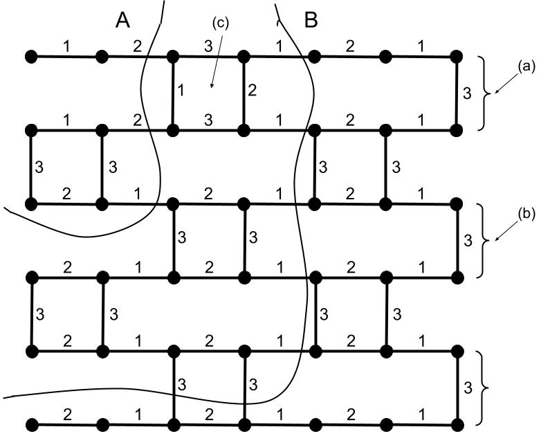
Figure 3: A visualization of the setup and proof of Lemma 4. The horizontal edges correspond to $\gamma_{1}$, and the vertical to $\gamma_{2}$. The edges pictured are those not given the color $4$. $A$ and $B$ are the regions indicated. The brackets show pairs in $P$. (c) shows the configuration of edges mentioned in condition 5 of the lemma statement. That configuration is used to swap parity for the element of $P$ labeled by (a), as shown. (b) labels an element of $P$ on which no parity swap is needed.

Lemma 4.

Suppose we have a partial edge coloring $c:(G(a,S^{\prime})\upharpoonright U)\rightarrow\{1,2,3,4\}$ which satisfies the following properties.

1. The domain of $c$ consists of all $\gamma_{2}$-edges, and all $\gamma_{1}$-edges meeting $A\cup B$.

2. $c$ gives all $\gamma_{1}$-edges the color $1$ or $2$, and all $\gamma_{2}$-edges the color $3$ or $4$.

3. Parallel $\gamma_{1}$-edges are always given the same color.

4. If $e,e^{\prime}$ are two edges in a single element of $\mathcal{F}$ meeting $A$, they get the same color iff the distance between them is odd. Likewise for $B$.

5. For every path from $A$ to $B$ consisting only of $\gamma_{1}$-edges, there is some edge $e$ on the path such that $e$ and its parallel edge, say $e^{\prime}$, are both disjoint from $A\cup B$, and both $\gamma_{2}$-edges from $e$ to $e^{\prime}$ have the color 3.

Then there is an (total) edge coloring $c^{\prime}:(G(a,S^{\prime})\upharpoonright U)\rightarrow\{1,2,3,4\}$ which agrees with $c$ on all edges meeting $A\cup B$.

Proof.

Essentially a proof by picture; See Figure 3.

First, the move from $c^{\prime}$ to $c$ will not change which edges get the color 4, so ignore those edges for the rest of the proof. We are left with a graph like the one in the figure. Fix a pair $\{f,f^{\prime}\}\in P$, so that we need to fill in the colors of the edges in $f$ and $f^{\prime}$ not meeting $A\cup B$. We would like to simply do this by continuing to alternate between the colors 1 and 2 on them, but we may run into parity issues.

By condition 4, this can only be the case along paths in $f$ or $f^{\prime}$ between $A$ and $B$. By condition 5, though, whenever we have such a situation, we can “borrow” the color 3 to indeed do a parity swap if necessary. Item (a) in the figure shows an example where this is the case, and item (b) an example where it is not. ∎

4.2.2 The standard generators

The remainder of Subsection 4.2 will involve reducing our desired result to several concrete cases. All will be handled using similar overall strategies, and ultimately relying on Lemma 4. The first of these will be when $S=\{\pm e_{i}\mid 1\leq i\leq d\}$ is the usual generating set for $\mathbb{Z}^{d}$. Fix this particular $S$ for now. We will cover this case carefully to illustrate our general strategy.

We first set up some additional terminology. Let $U\subset U^{\prime}$ be subsets of some fixed $\mathbb{Z}^{d}$-orbit $U^{\prime\prime}$, and let $c:(G(a,S)\upharpoonright U^{\prime})\rightarrow\{1,\ldots,2d\}$ an edge coloring. Let $x_{0}\in U^{\prime\prime}$. We say that $c$ follows protocol $x_{0}$ on $U$ if for each edge $(x,e_{i}\cdot x)$ of $G(a,S)\upharpoonright U^{\prime}$ meeting $U$, $c$ gives this edge the color $2i-1$ if $a_{i}$ is even and $2i$, otherwise, where $(a_{1},\ldots,a_{d})\in\mathbb{Z}^{d}$ is the unique element such that $(a_{1},\ldots,a_{d})\cdot x_{0}=x$. Of course, it is always possible to $2d$-edge color a given subset of $U^{\prime\prime}$ following a given protocol. Also note the choice of $x_{0}$ only matters modulo the action of the subgroup $(2\mathbb{Z})^{d}$.

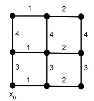
Figure 4: A partial coloring for $d=2$ following protocol $x_{0}$.

It is clear that if $U$ and $V$ are two disjoint subsets of $U^{\prime\prime}$ and $c$ is a coloring of $G(a,S)\upharpoonright(U\cup V)$ following a given protocol, then $c$ can be extended to a coloring of all of $G(a,S)\upharpoonright U^{\prime\prime}$ following that same protocol. We now need to see what to do when $U$ and $V$ follow different protocols.

Lemma 5.

Let $1\leq i\leq d$. Suppose $U\subset U^{\prime\prime}$ and $c$ is an edge coloring of $B(U,1)$ following some protocol $x_{0}$ on $A(U,0,1)$. Then we can extend $c$ to a coloring of $G\upharpoonright B(U,5)$ which still follows protocol $x_{0}$ on $A(U,0,1)$, but also follows protocol $e_{i}\cdot x_{0}$ on $A(U,4,5)$.

Proof.

First, color any edges in $B(U,5)$ meeting $A(U,4,5)$ or $A(U,0,1)$ as dictated by the protocols $e_{i}\cdot x_{0}$ and $x_{0}$ respectively. These two protocols agree about how to color edges corresponding to $e_{j}$ for $j\neq i$, so tentatively color all these edges in $A(U,0,5)$ as dictated by these protocols.

We need to fill in the colors for the remaining $e_{i}$ edges: those contained in $A(U,1,4)$. Since $d>1$, fix some $j\neq i$. Observe that we can do this by applying Lemma 4 with $\gamma_{1}=e_{i}$, $\gamma_{2}=e_{j}$, $A=A(U,0,1)$, $B=A(U,4,5)$ and the colors 1,2,3, and 4 replaced with $2i-1,2i,2j-1$, and $2j$ respectively. All conditions other than 5 are immediately apparent. $P$ will pair up any two adjacent $e_{i}$ orbits whose connecting edges all get the color 3. That is, it will consist of pairs of the form $f,e_{j}\cdot f$ for which $f$ contains a point $(a_{1},\ldots,a_{d})\in x_{0}$ with $a_{j}$ even. Then, for condition 5, any edge $e$ such that both $e$ and its parallel edge are contained in $A(U,1,4)$ will work. 4 is large enough so that we are always guaranteed the existence of such an edge, so we are done. Note that the picture here will look like that in Figure 2. ∎

Lemma 6.

Suppose $U\subset U^{\prime\prime}$ and $c$ is an edge coloring of $G(a,S)\upharpoonright U$ following some protocol $x_{0}$. Then we can extend $c$ to a coloring of $G(a,S)\upharpoonright B(U,4d+1)$ which still follows protocol $x_{0}$ on $U$, but also follows some arbitrary second protocol, say $x_{1}$, on $A(U,4d,4d+1)$.

Proof.

This is an obvious induction using Lemma 5. ∎

Lemma 7.

Suppose $U,V\subset U^{\prime\prime}$, the $G(a,S)$-path distance between $U$ and $V$ is greater than $4d+1$, and $c$ is an edge coloring of $G\upharpoonright(U\cup V)$ which follows some protocols $x_{0}$ and $x_{1}$ on $U$ and $V$ respectively. Then we can extend $c$ to a coloring of $U^{\prime\prime}$ which still follows those protocols on $U$ and $V$ respectively.

Proof.

First, extend $c$ to $B(U,4d+1)$ as in Lemma 6. Then color the rest of the edges in $U^{\prime\prime}$ following protocol $x_{1}$. ∎

Now, thanks to the fact $\textnormal{asi}_{B}(G(a,S))=1$, Lemma 7 is enough:

Lemma 8.

With $S$ the standard generating set, $\chi_{B}(G(a,S))=|S|=2d$.

Proof.

Let $N=8(d+1)$. Let $X=U_{1}\sqcup V$ be a Borel partition witnessing $\textnormal{asi}_{B}(G(a,S))=1$ for this value of $N$. Let $V_{1}=X\setminus B(U_{1},4d+1)$. Arguing as in the proof of Lemma 1, we can conclude that every injective $G(a,S)$-ray passes through $V_{1}$. Thus, by König’s lemma, the connected components of $G(a,S)\upharpoonright(X\setminus V_{1})$ are still all finite. $G(a,S)\upharpoonright V_{1}$ also has only finite connected components since $V$ did. Likewise for $U_{1}$ and its complement. See Figure 5 to see how these sets might be arranged.

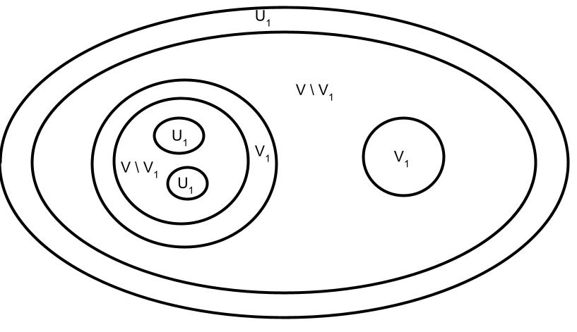
Figure 5: A typical arrangement of the sets in the proof of Lemma 8 for $d=2$.

Thus, as in the proof of Lemma 2, we may Borel $2d$-edge color $G(a,S)\upharpoonright U_{1}$ so that a consistent protocol is followed within each $G(a,S)\upharpoonright(X\setminus V_{1})$ component, and Borel $2d$-edge color $G(a,S)\upharpoonright V_{1}$ so that a consistent protocol is followed within each $G(a,S)\upharpoonright(X\setminus U_{1})$-component.

Now let $C$ be a $G(a,S)\upharpoonright(V\setminus V_{1})$-component. Let $V_{2}$ be the union of the $V_{1}$-components meeting $C$,and $U_{2}$ the union of the $U_{1}$-components meeting $C$. $V_{2}$ is contained in a single $(X\setminus U_{1})$-component, and hence is colored using a consistent protocol , and likewise for $U_{2}$. Thus, by Lemma 7 (note that the path distance between $U_{2}$ and $V_{2}$ is more than $4d+1$), we can find a coloring of $C\cup U_{2}\cup V_{2}$ which still follows the original protocols set for $U_{2}$ and $V_{2}$ on those sets. Since $C$ is always finite, we can in a Borel fashion do this simultaneously for every such $C$, and by construction this does not cause any color conflicts. ∎

Since the remaining cases we cover will be handled very similarly to this one, we will not go over these details for each one. Instead we will content ourselves in each one with establishing some appropriate notion of “protocol”, and using Lemma 4 to at least sketch some analogue of Lemma 6 saying different such protocols can be transitioned between in a bounded neighborhood.

For example, one case we will need to address is $d=2$,

$$S=\{\pm(a_{1},0),\ldots,\pm(a_{n},0),\pm(0,b_{1}),\ldots,\pm(0,b_{m})\}$$

for $n,m>1$ and the $a_{i}$’s and $b_{i}$’s arbitrary positive integers (possibly with repeats).

Let $U^{\prime\prime}$ be a $\mathbb{Z}^{2}$-orbit as before. In this setting, for $x_{0}\in U^{\prime\prime}$, protocol $x_{0}$ will dictate that if $x\in U^{\prime\prime}$ with $x=(g_{1},g_{2})\cdot x_{0}$, then the edge $(x,(a_{i},0)\cdot x)$ gets the color $2i-1$ if $g_{1}\in[0,a_{i})$ (mod $2a_{i}$) and the color $2i$ otherwise, and likewise for the $(0,b_{j})$ generators.

The technique in this setting for transitioning between different given protocols is exactly like that in the standard generator case. Thus we have:

Lemma 9.

With $d=2$ and $S$ as above, $\chi_{B}(G(a,S))=|S|$.

Of course, there is nothing special here about $d=2$, but it makes for shorter notation and we will not need the higher dimensional versions of this case.

4.2.3 $\mathbb{Z}^{2}$ with three generators, subcase 1

We now consider cases of the form $d=2$, $S=\{\pm(n,0),\pm(0,n),\pm(b_{1},b_{2})\}$, where $n,b_{1}$, and $b_{2}$ are positive integers. Of course, we may assume $n,b_{1}$, and $b_{2}$ do not share any common factors. Fix such an $S$ for the time being.

First consider the sub-case $n=1$. This will split into two further sub-cases, depending on the parity of $b_{1}$ and $b_{2}$. For the first, suppose one of the $b$’s is even. WLOG let us say it is $b_{2}$.

Let $U^{\prime\prime},x_{0}$ as before. Protocol $x_{0}$ will assign the colors $1,2,3$, and $4$ to the $(1,0)$ and $(0,1)$-edges exactly as in the standard generators case. It will also assign the color 5 to edges of the form $((a_{1},a_{2})\cdot x_{0},(a_{1}+b_{1},a_{2}+b_{2})\cdot x_{0})$ if $a_{1}\in[0,b_{1})$ (mod $2b_{1}$) and 6 to such edges otherwise.

We already know how to alter the protocol used for the $(1,0)$ and $(0,1)$-edges, so we need to consider the $(b_{1},b_{2})$ edges. Given a coloring following some protocol $x_{0}$, though, consider the subgraph consisting of $(b_{1},b_{2})$-edges along with all $(0,1)$-edges colored $3$. Since $b_{2}$ is even, the resulting picture will look exactly like the one from the standard generators case (Figure 2), but with the colors 5 and 6 in place of 1 and 2. That is, in the Language of Lemma 4 with $\gamma_{1}=(b_{1},b_{2})$ and $\gamma_{2}=(0,1)$, we can chose $P$ so that for any $\{f,f^{\prime}\}\in P$, all $(0,1)$-edges from $f$ to $f^{\prime}$ have the color $3$. Thus by the Lemma we can swap parity for the 5’s and 6’s for such pairs as necessary. For example, if we want to transition to the protocol $(1,0)\cdot x_{0}$, we do this swap for all pairs $\{f,(0,1)\cdot f\}\in P$ for which $f$ contains a point of the form $(a_{1},a_{2})\cdot x_{0}$ with $a_{1}$ a multiple of $b_{1}$, and leave the parity unchanged on all other pairs.

For the second sub-case, suppose both $b_{1}$ and $b_{2}$ are odd. Our notion of protocol will be defined identically as in the previous subcase, but altering protocol for the $(b_{1},b_{2})$-edges will be more difficult.

Suppose $U\subset U^{\prime\prime}$ is some finite subset, and we have an edge coloring $c$ on $B(U,1)$ which follows some protocol $x_{0}$. Since Lemma 4 allows us to control parity separately in each pair of $\gamma_{1}$-orbits in $P$, we can, as in the standard generators case, extend $c$ to an edge coloring on $B(U,5)$, but this time shifting parity on every other adjacent pair of $(0,1)$-orbits. Call this new pattern of edge colors the alternating protocol $x_{0}$.

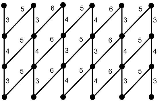
Figure 6: A picture of the $(0,1)$ and $(1,1)$ edges in a coloring using an alternating protocol. Here $b_{1}=b_{2}=1$.

Figure 6 shows the result of this new protocol in the case $b_{1}=b_{2}=1$. Consider the result when taking from this new protocol only the $(b_{1},b_{2})$-edges and the $(0,1)$-edges colored 3. Since $b_{1}$ and $b_{2}$ are odd, the resulting picture looks exactly like that in Figure 3, but with the colors 5 and 6 in place of the colors 1 and 2. It therefore follows from Lemma 4 that for some large enough $N$ (but only depending on $b_{1}$ and $b_{2}$), we will be able to extend $c$ further to an edge coloring on $B(U,N)$ which, on $A(U,N-1,N)$, follows alternating protocol $x_{0}$ for the $(1,0)$ and $(0,1)$-edges, but follows protocol $(1,0)\cdot x_{0}$ for the $(b_{1},b_{2})$-edges. As in the previous subcase, this will involve switching parity along exactly those $(b_{1},b_{2})$-orbits which meet a point of the form $(a_{1},a_{2})\cdot x_{0}$ for which $a_{1}$ is a multiple of $b_{1}$. Finally, we extend this to a coloring on $B(U,N+5)$ while undoing the parity shifts in the $(0,1)$-orbits, ending up with a coloring which, on $A(U,N+4,N+5)$, follows protocol $x_{0}$ for the $(1,0)$ and $(0,1)$-edges, but $(1,0)\cdot x_{0}$ for the $(b_{1},b_{2})$-edges. This is exactly what we wanted, so this case is done.

4.2.4 $\mathbb{Z}^{2}$ with three generators, subcase 2

Finally, we remove the assumption $n=1$. Then, since we assumed there were no common divisors, WLOG $n$ does not divide $b_{2}$. Our notion of protocol for the $(n,0)$ and $(0,n)$ edges will be defined as in the Lemma 9 case. For the $(b_{1},b_{2})$ edges, it will be defined exactly as in the previous subcases.

Thus, we can alter protocol for the $(n,0)$ and $(0,n)$-edges as we did in Lemma 9, so once again it suffices to see how to shift parity for the $(b_{1},b_{2})$-edges.

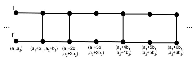
Figure 7: A visualization of the $n>1$ case. The horizontal edges are the $(b_{1},b_{2})$-edges, while the vertical ones are the $(0,n)$-edges colored 3. The label $(g_{1},g_{2})$ for a point is shorthand for $(g_{1},g_{2})\cdot x_{0}$. Whether or not a vertical edges touching some $(g_{1},g_{2})$ is included depends on the value of $g_{2}$ mod $2n$.

We wish to apply Lemma 4 with $\gamma_{1}=(b_{1},b_{2})$, $\gamma_{2}=(0,n)$, and the colors 5 and 6 in place of 1 and 2. Suppose we have some edge coloring of $G(a,S)\upharpoonright U^{\prime\prime}$ following protocol $x_{0}$. In the language of Lemma 4, consider 2 adjacent $(b_{1},b_{2})$-orbits $f$ and $f^{\prime}=(0,n)\cdot f$. Note that as in the previous subcases, condition 3 of the lemma is automatic by our choice of protocol for the $(b_{1},b_{2})$-edges. Thus to apply the lemma in the way we want, It would suffice to find an $N$ (depending only on $n,b_{1}$, and $b_{2}$) such that for every path in $f$ of length $N$, there is some edge $e$ in the path satisfying condition 5 of the lemma. That is, such that both $(0,n)$-edges from $e$ to $f^{\prime}$ get the color 3.

Let $(a_{1},a_{2})\cdot x_{0}$ be an arbitrary point in $f$, so that the points on $f$ are those of the form $(a_{1}+kb_{1},a_{2}+kb_{2})\cdot x_{0}$ for $k\in\mathbb{Z}$. By definition of our protocol, the edge from such a point to $f^{\prime}$ will get the color 3 if and only if $a_{2}+kb_{2}\in[0,n)$ (mod $2n$).

Our problem thus reduces to the following number theoretic one. Given that $n\not|\ b_{2}$, find $N$ large enough so that for any $a_{2}\in\mathbb{Z}$, there is some $k\in[0,N]$ such that $a_{2}+kb_{2}$ and $a_{2}+(k+1)b_{2}$ are both in the range $[0,n)$ (mod $2n$). Since everything is modulo $2n$, it just suffices to show that we can find some such $k\in\mathbb{N}$, and then we can take $N=2n$. Assume that $b_{2}\in(0,n)$ (mod $2n$), as the case $b_{2}\in(n,2n)$ (mod $2n$) will follow from a similar argument.

Now let $q=\gcd(b_{2},2n)<n$. Then there will always be a $k$ such that $a_{2}+kb_{2}\in[0,q)$ (mod $2n$). Also, since we have assumed $b_{2}\in(0,n)$ (mod $2n$), we must actually have $b_{2}\in[q,n-q]$ (mod $2n$). Then $a_{2}+(k+1)b_{2}$ is in the range $[0,n)$ (mod $2n$) as desired.

Let’s record the result of Subsubsections 4.2.3 and 4.2.4 together:

Lemma 10.

With $d=2$, $S=\{\pm(n,0),\pm(0,n),\pm(b_{1},b_{2})\}$ for some $b_{1},b_{2},n>0$ $\chi_{B}^{\prime}(G(a,S))=|S|=6$.

4.2.5 Combining the cases

Finally, we are ready to finish the proof for general $d$ and $S$.

Proof.

Let $S=\{\pm\gamma_{1},\ldots,\pm\gamma_{n}\}$, and let $S^{\prime}=\{\gamma_{1},\ldots,\gamma_{n}\}$. We define an equivalence relation $\sim$ on $S^{\prime}$ which sets two generators as equivalent if one is a scalar multiple of the other. Equivalently, if the subgroup they generate is cyclic. Let $C_{1},\ldots,C_{m}$ list the classes in $S^{\prime}/\sim$. Note that we must have $m\geq d>1$.

Because of this, we can partition the $C_{i}$’s into sets of size 2 and 3. It now suffices to show that given an element of this partition $\{C_{i_{j}}\mid 1\leq j\leq r\}$, where $r\in\{2,3\}$, we can Borel color the edges in $G(a,\pm\bigcup_{j}C_{i_{j}})$ using $|\pm\bigcup_{j}C_{i_{j}}|$ colors.

First consider the case $r=2$. For notational convenience, take $i_{j}=j$ for $j=1,2$. Let $\Gamma=\langle C_{1},C_{2}\rangle\cong\mathbb{Z}^{2}$. Then $(\Gamma,\pm(C_{1}\cup C_{2}))$ is isomorphic as a marked group to $\mathbb{Z}^{2}$ with a set of generators of the form covered in Lemma 9, so that Lemma says this case is done.

Next consider the case $r=3$, and again take $i_{j}=j$ for $j=1,2,3$. We would like to reduce to the case where $C_{1},C_{2}$, and $C_{3}$ are all singletons. Suppose, for instance that $C_{1}$ includes at least two elements, and let $\delta_{1}$ be one. Pick some $\delta_{2}$ from $C_{2}$. Then we can $4$-edge color $G(a,\{\pm\delta_{1},\pm\delta_{2}\})$ by the previous paragraph. We are left with $C_{1}-\{\delta_{1}\},C_{2}-\{\delta_{2}\}$, and $C_{3}$. Note that $C_{1}-\{\delta_{1}\}$ is still nonempty. If $|C_{2}|=1$, then we have reduced to the previous paragraph. If not, and one of our three sets still contains more than one element, repeat this.

Thus we have our reduction. Let $C_{i}=\{\delta_{i}\}$ for $i=1,2,3$. Now by definition of $\sim$, $\Gamma:=\langle\delta_{1},\delta_{2},\delta_{3}\rangle$ is isomorphic to either $\mathbb{Z}^{2}$ or $\mathbb{Z}^{3}$.

In the latter case, $(\Gamma,\{\pm\delta_{1},\pm\delta_{2},\pm\delta_{3}\})$ is isomorphic as a marked group to $\mathbb{Z}^{3}$ with its standard generators, so by Lemma 8 we are done.

In the former case, we can write $n\delta_{3}=b_{1}\delta_{1}+b_{2}\delta_{2}$ for some $n,b_{1},b_{2}\neq 0$. Then $(\Gamma,\{\pm\delta_{1},\pm\delta_{2},\pm\delta_{3}\})$ is isomorphic as a marked group to $\mathbb{Z}^{2}$ with the generating set from Lemma 10. (Send $\delta_{1}$ to $(n,0)$, $\delta_{2}$ to $(0,n)$, and $\delta_{3}$ to $(b_{1},b_{2})$.) We can also assume $n,b_{1},b_{2}>0$ by replacing the $\delta$’s with their inverses if necessary. Thus by the lemma, we are done. ∎

4.3 Free rank 1

In this subsection we complete the proof of Statement 2 of Theorem 2. For the discrete part of the statement, since we can use Lemma 3 with $\Delta=\Delta^{\prime}$, it suffices to prove $\chi^{\prime}(G(a,S))=|S|$ when $\Gamma=\mathbb{Z}$, but where we now allow multiplicity for generators. This is obviously the case, though.

We thus turn to the Borel part of the statement, We need to show that if $\Delta$ has even order, then $\chi_{B}^{\prime}(G(a,S))=|S|$. As in the proof of Statement 1, we can start by finding an index 2 subgroup $\Delta^{\prime}\leq\Delta$, and then use Lemma 3 to reduce to the case where $\Delta=\mathbb{Z}/2$, but where we now allow multiplicity for generators in $S$. For the rest of the subsection, assume $(\Gamma,S)$ has this form. We will sometimes write “$\mathbb{Z}$” to refer to the subgroup $\{0\}\times\mathbb{Z}\leq\Gamma$.

We start with the special case where $(1,0)\in S$. (Recall we are writing $\Gamma=\mathbb{Z}/2\times\mathbb{Z}$. For example this element has order 2.)

Lemma 11.

If $(1,0)\in S$, $\chi_{B}^{\prime}(\Gamma,S)=|S|$.

Proof.

This follows immediately from Corollary 2 with $\Delta=\mathbb{Z}/2$. ∎

Thus, from now on assume $(1,0)\not\in S$. Then we can write $S=S^{\prime}\sqcup-S^{\prime}$, where $S^{\prime}$ consists of all pairs $(\epsilon,n)\in S$ for which $n>0$. Our proof will be organized as follows: The elements $(\epsilon,n)\in S^{\prime}$ will be organized into 4 categories corresponding to the value of $\epsilon$ and the parity of $n$. We will consider these categories roughly one at a time, for each establishing a suitable notion of protocol as in the previous subsection, and demonstrating how to transition between protocols.

These transitions will always be accomplished by an argument in the style of Lemma 4. That lemma was stated in the context of $\mathbb{Z}^{d}$, but in this context its terminology still makes sense and its conclusion still holds.

4.3.1 Generators from $2\mathbb{Z}+(0,1)$ and $\mathbb{Z}+(1,0)$

Let’s begin. There must be some element $(\epsilon,n)\in S^{\prime}$ for which $n$ is odd. Note that there is an automorphism of $\Gamma$ exchanging $(1,1)$ and $(0,1)$. This will send $(\epsilon,n)$ to $(1-\epsilon,n)$, so we may assume $S^{\prime}$ has an element of the form $(0,n)$ for $n$ odd. Then it must also have an element of the form $(1,m)$. Fix such elements for the rest of the proof.

We start by examining how to color the $(0,n)$ and $(1,m)$-edges. Let $U^{\prime\prime}$ be a $\Gamma$-orbit, and $x_{0}\in U^{\prime\prime}$. For any generator of the form $(1,m^{\prime})$, protocol $x_{0}$ will dictate that edges of the form $(x,(1,m^{\prime})\cdot x)$ get the color 3 if $x$ and $x_{0}$ are in the same $\mathbb{Z}$-orbit, and 4 if they are not. We will always use such protocols for such edges, so we will need to be able to transition between the protocols $x_{0}$ and $(1,0)\cdot x_{0}$. Call these protocols two sided protocols.

For any generator of the form $(0,n^{\prime})$ for $n^{\prime}$ odd, a coloring of the $(0,n^{\prime})$-edges on $\mathbb{Z}\cdot x_{0}$ will be said to follow the odd protocol $x_{0}$ if $(x,(0,n^{\prime})\cdot x)$ gets the color $1$ or $2$ according to whether the integer $a^{\prime}$ such that $x=(0,a^{\prime})\cdot x_{0}$ is even or odd respectively. Note that this protocol does indeed give a coloring since $n^{\prime}$ is odd. Now a coloring of the $(0,n^{\prime})$-edges on $U^{\prime\prime}$ will be said to follow the parallel protocol $x_{0}$ if it follows the odd protocols $x_{0}$ and $(1,0)\cdot x_{0}$ on $\mathbb{Z}\cdot x_{0}$ and $(\mathbb{Z}+(1,0))\cdot x_{0}$ respectively, and the alternating protocol $x_{0}$ if it follows the odd protocols $x_{0}$ and $(1,1)\cdot x_{0}$ on $\mathbb{Z}\cdot x_{0}$ and $(\mathbb{Z}+(1,0))\cdot x_{0}$ respectively. Whichever of these protocols is used, we will need to be able to transition between that corresponding to $x_{0}$ and that corresponding to $(0,1)\cdot x_{0}$.

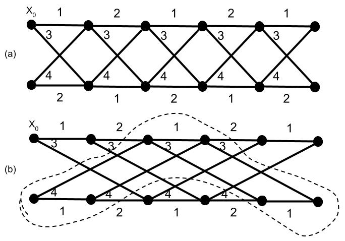
Figure 8: (a): A drawing of a coloring following protocol $x_{0}$ in the case $n=m=1$. Note that the $(0,1)$-edges use the alternating protocol. (b): Same, but now with $m=2$. Note that now the $(0,1)$-edges use the parallel protocol. The dotted line sections off a pair of adjacent $(1,m)$ orbits. This makes it clear that they follow the necessary hypotheses to apply Lemma 4.

Now, returning to our fixed $(0,n)$ and $(1,m)$, if $m$ is odd, we will use alternating protocols for the $(0,n)$-edges, and if $m$ is even, we will use parallel protocols. Pictures of both cases are shown in Figure 8.

We now see how to shift these protocols. To shift the protocol used for the $(0,n)$-edges, We want to apply Lemma 4 with $\gamma_{1}=(0,n)$ and $\gamma_{2}=(1,m)$. Our partition $P$ will group together two $(0,n)$-orbits $f$ and $(1,m)\cdot f$ if $f$ is in the same $\mathbb{Z}$-orbit as $x_{0}$, This, way, by our use of the two sided protocol $x_{0}$ for the $(1,m)$-edges, the $(1,m)$-edges connecting $f$ and $(1,m)\cdot f$ will always have the color 3, which will give condition 5 in the lemma. Our use of an alternating or parallel protocol with respect to the parity of $m$ ensures condition 3 is satisfied. Thus, for every such pair, we can flip parity for the $(0,n)$-edges. Doing this for each pair transitions us from protocol $x_{0}$ to protocol $(0,1)\cdot x_{0}$ for the $(0,n)$-edges, as desired.

The $(1,m)$-edges work out similarly. We now want to apply the lemma with $\gamma_{1}=(1,m)$ and $\gamma_{2}=(0,n)$. Observe that it is still possible to define the partition $P$ so that if $f$ and $f^{\prime}$ are $(1,m)$-orbits grouped together, the edges between them all get color 1. Part (b) of Figure 8 gives an example how to do this. The general idea is that we have chosen our protocol for the $(0,n)$-edges so that our coloring of them descends to one of the quotient of our graph by the subgroup $\langle(1,m)\rangle$, so we can just group together orbits just in case they are related in this quotient by an edge of color 1. This takes care of condition 5, and condition 3 comes from our use of a two sided protocol for the $(1,m)$-edges.

A remark for clarity: While we have defined the above protocols all relative to a single base point $x_{0}$, when making transitions we never need to assume the base point used for the $(0,n)$-edges is the same as that used for the $(1,m)$-edges. This is important, as to actually turn these protocol shifting arguments into a Borel edge coloring, we need to be able to shift the protocol for each generator one at a time. This will continue to be the case throughout this subsection, and we will not remark on it further.

If $S^{\prime}$ has additional elements of the form $(0,n^{\prime})$ for $n^{\prime}$ odd, we can color them using alternating or parallel protocols (but with new colors) according to the parity of $m$, and as above use the $(1,m)$-edges to make transitions. Likewise, if $S^{\prime}$ has additional elements of the form $(1,m^{\prime})$ with $m^{\prime}\cong m$ (mod 2), we can color them using two sided protocols and use the $(0,n)$-edges (since they will be colored using the correct protocol to work with $m^{\prime}$) to make transitions.

4.3.2 Generators from $\mathbb{Z}+(1,0)$ with different parity

A difficulty arises if $S^{\prime}$ contains elements of the form $(1,m^{\prime})$ for $m^{\prime}$ both odd and even. If this is the case, let us decide that our fixed $m$ from before is even, so that in the previous paragraph we have handled all $(1,m^{\prime})$’s for $m^{\prime}$ even. We now need to see what to do with generators of the form $(1,b)$ for $b$ odd.

Fix such a generator. When coloring the $(1,b)$-edges according to our usual two sided protocols, let us use the colors 5 and 6 in place of 3 and 4 respectively. We will divide our argument into two cases depending on whether $n$ divides $b$. Suppose first that $n$ does divide $b$.

By working separately on each $\mathbb{Z}/2\times n\mathbb{Z}$-orbit, we can assume $n=1$. Then, Figure 9 shows how to use the $(0,1)$-edges to transition between our two possible protocols for the $(1,b)$-edges in the case $b=3$. It should be clear how this pattern can be continued to other $b$.

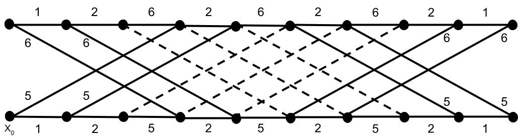
Figure 9: A demonstration of how to change protocol for the $(1,b)$ edges when $n=1$ and $b=3$. Note that the $(0,1)$-edges use a parallel protocol since $m$ is even. The dashed diagonal lines all get the color 1. Observe that, on the left side of the figure, the $(1,b)$-edges follow two sided protocol $x_{0}$, while on the right they follow two sided protocol $(1,0)\cdot x_{0}$, as desired.

Next suppose that $n$ does not divide $b$. Let $q=\gcd(n,b)=\gcd(n,2b)<n$. The following will be important for a soon to come number theoretic argument.

Lemma 12.

$b+m$ and $b-m$ do not both lie in the interval $(n-q,n+q)$ (mod $2n$).

Proof.

Suppose not. Then, since $m+b$ and $m-b$ differ by $2b$, a multiple of $q$, they must either be equal mod $2n$, or differ by exactly $q$ mod $2n$.

In the former case, we get $2b=0$ (mod $2n$), which contradicts $n$ not dividing $b$.

In the latter case, we get $2b=\pm q$ (mod $2n$), but note that $q$ must be odd, so this is also a contradiction. ∎

Assume then that $b-m$ does not lie in this interval mod $2n$. The argument in the case where $b+m$ is not in this interval will be similar. Assume further that $b-m\in[0,n-q]$ (mod $2n$), as the argument in the case where it is in $[n+q,2n]$ (mod $2n$) will again be similar.

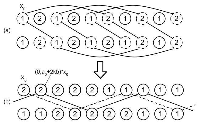
Figure 10: A demonstration of how to change protocol for the $(1,b)$ edges when $n=5$,$m=2$, and $b=3$. For visual clarity, the label of a vertex $x$ refers to the color of the edge $(x,(0,n)\cdot x)$. (a): Step 1 of the procedure. The dashed vertices are those included in one of the $(0,n)$-orbits along which parity is changed. The edges drawn are the $(0,n)$ and $(1,m)$-edges involved in making that change for these orbits. (b): The effects of step 1, along with a pair of $(1,b)$-orbits of the form $f,(0,n)\cdot f$ from step 2. The solid and dashed lines are the edges from $f$ and $(0,n)\cdot f$ respectively. A vertex $(0,a_{0}+2kb)\cdot x_{0}$ of $f$ which satisfies the number theoretic condition from step 2 is highlighted.

Now, our transition will occur in three steps. In step 1, we will use the $(1,m)$-edges to put the colors of the $(0,n)$-edges in a more useful arrangement. Recall that, in the previous subsubsection, to swap protocols for the $(0,n)$-edges, we divided the $(0,n)$-orbits into pairs of the form $f,(1,m)\cdot f$, for $f\subset\mathbb{Z}\cdot x_{0}$, and saw we could swap parity for the colors 1 and 2 along each orbit. In our step 1 for this case, let us only swap parity on those pairs for which $(0,2l)\cdot x_{0}\in f$, for $l=0,1,\ldots,(n-1)/2$. This is demonstrated in Figure 10, with the result of these swaps shown in part (b) of the figure: The $(0,n)$-edges in each $\mathbb{Z}$-orbit are now colored with 1 and 2, but in alternating blocks of length $n$. In the orbit $\mathbb{Z}\cdot x_{0}$, a block of color $2$ starts at the edge $(x_{0},(0,n)\cdot x_{0})$, while in the other orbit $(\mathbb{Z}+(1,0))\cdot x_{0}$, a block of color 2 starts at the edge $((1,m)\cdot x_{0},(1,m+n)\cdot x_{0})$. That is, the patterns in these two orbits are “offset by $m$”.

In step 2, we will make an argument similar to that from Subsubsection 4.2.4. Partition the $(1,b)$-orbits into pairs of the form $f,f^{\prime}=(0,n)\cdot f$, which is possible as $(0,n)$ has even order in the quotient $\Gamma/\langle(1,b)\rangle$, since $n$ is odd. One such pair is depicted in part (b) of Figure 10. Such an $f$ can be described by a vertex of the form $(0,a_{0})\cdot x_{0}$, so that the elements of $f\cap\mathbb{Z}\cdot x_{0}$ are those of the form $(0,a_{0}+2kb)\cdot x_{0}$ for $k\in\mathbb{Z}$. Each such point determines a pair of parallel edges $e:=((0,a_{0}+2kb)\cdot x_{0},(1,a_{0}+2kb+b)\cdot x_{0})$ and $(0,n)\cdot e$ in $f$ and $f^{\prime}$ respectively. If the two $(0,n)$-edges connecting $e$ and $(0,n)\cdot e$ both have the color 2, then this pair of edges will witness condition 5 from Lemma 4, so we will be able to change parity along $f$ and $f^{\prime}$ as desired.

By our previous description of the effects of step 1, this will be the case if both $a_{0}+2kb$ and $a_{0}+2kb+b-m$ are in the interval $[0,n)$ (mod $2n$), so we want to show that given $a_{0}$, we can always find a $k$ such that this is the case. Well, since $q=\gcd(n,2b)$, we can find a $k$ such that $a_{0}+2kb\in[0,q)$ (mod $2n$), and then since are working under the assumption $b-m\in[0,n-q]$ (mod $2n$), we will also have $a_{0}+2kb+b-m\in[0,n)$ (mod $2n$) as desired. Thus we can swap parity along all $(1,b)$-orbits as desired.

Finally, in step 3, we reverse step 1. That is, we swap parity along all the pairs of $(0,n)$-orbits used in step 1 to return to a coloring of the $(0,n)$-edges which follows parallel protocol $x_{0}$.

4.3.3 Generators from $2\mathbb{Z}$

The only generators left to consider are those of the form $(0,b)\in S^{\prime}$ for $b$ even. Fix such a $b$. In our treatment of these, we will often work in one $\mathbb{Z}$-orbit at a time. We therefore start by establishing a key lemma in the setting of $\mathbb{Z}$-actions. For this, we’ll start with a purely combinatorial game.

Suppose we have a finite graph consisting of a single path $v_{0},\ldots,v_{l}$ of length $l$, where $v_{i}$ and $v_{j}$ are adjacent if and only if $|i-j|=1$. Suppose the vertices of this path are labeled with two colors, say 5 and 6. In one move, we are allowed to pick two adjacent vertices of the same color, and change both of their colors. Some examples of moves are shown in Figure 11.

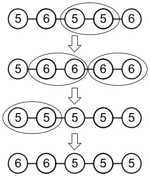
Figure 11: An example of a sequence of moves in our game with $l=4$. When a pair of adjacent vertices is circled, it indicates that our next move will be changing the color on those vertices. We sometimes draw two moves as occuring in a single step if the pairs of vertices they involve are disjoint. Note also that this sequence provides and example for Lemma 13.

Lemma 13.

If either $l$ is even and $v_{0}$ and $v_{l}$ have different colors, or $l$ is odd is $v_{0}$ and $v_{l}$ have the same color, then there is a sequence of moves which result in $v_{0}$ and $v_{l}$ switching their colors, but all other vertices keeping the same color.

Proof.

We proceed by strong induction on $l$. The base case $l=1$ is clear.

Now suppose $l>1$. By hypothesis, there must be some pair $v_{i},v_{i+1}$ of adjacent vertices with the same color. Pick the pair with $i$ minimal. Our first move will be changing the colors on this pair.

If $i=0$, then $v_{0}$ is now the color we want it to be. If $i>0$, then we now want to change the colors on $v_{0}$ and $v_{i}$, but leave the vertices between them the same color. By the minimality of $i$, though in our initial coloring, $v_{0}$ and $v_{i}$ had the same color if and only if $i$ is even. Thus, after our first move, the path from $v_{0}$ to $v_{i}$ satisfies the hypotheses of the lemma, so by the inductive hypothesis, we can indeed change the colors of $v_{0}$ and $v_{i}$ and leave the vertices between them the same color.

Essentially the same thing happens for the path from $v_{i+1}$ to $v_{l}$. We’d like to check that in our initial coloring, $v_{i+1}$ and $v_{l}$ had the same color if and only if $l-(i+1)$ is even. We know as in the previous paragraph that $v_{i+1}$ has the same color as $v_{0}$ if and only if $i+1$ is odd. Also by hypothesis, $v_{l}$ has the same color as $v_{0}$ if and only if $l$ is odd. Combining these gives us what we want. ∎

We now turn to the promised $\mathbb{Z}$-action setting. Let $X^{\prime}$ be an orbit of some $\mathbb{Z}$-action $a^{\prime}$. Let $n^{\prime},b^{\prime}>0$ with $n^{\prime}$ odd, $b^{\prime}$ even, and furthermore assume $\gcd(n^{\prime},b^{\prime})=1$. Consider edge colorings of the graph $G(a^{\prime},\{\pm n^{\prime},\pm b^{\prime}\})\upharpoonright X^{\prime}$.

Since $n^{\prime}$ is odd, let us always use the odd protocol for coloring the $n^{\prime}$-edges with the colors 1 and 2.

Now a 2 coloring of the $b^{\prime}$-edges, say with the colors 5 and 6, is completely determined by the colors it gives to the edges $(k\cdot x_{0},(k+b^{\prime})\cdot x_{0})$ for $k=0,\ldots,b^{\prime}-1$, where here $x_{0}\in X^{\prime}$ is as before some fixed base point. Consider this sequence of colors, say $c(0),\ldots,c(b^{\prime}-1)$, as a map $c:\mathbb{Z}/b^{\prime}\rightarrow\{5,6\}$. We will say this coloring follows protocol $(x_{0},c)$. We will also say $c$ is the code of this coloring relative to $x_{0}$. For $\alpha\in\{5,6\}$, let $\neg\alpha$ denote the element of $\{5,6\}$ not equal to $\alpha$. Define the map $\overline{c}:\mathbb{Z}/(2b^{\prime})\rightarrow\{5,6\}$. By $\overline{c}(k)=c(k)$ if $k\in[0,b^{\prime})$ (mod $2b^{\prime}$) and $\overline{c}(k)=\neg c(k)$ otherwise. $\overline{c}$ will be called the double code of our coloring relative to $x_{0}$. Of course, it carries the same information as $c$, but will sometimes be easier to work with. The point is that $\overline{c}(k)$ is the color received by the edge $(k\cdot x_{0},(k+b^{\prime})\cdot x_{0})$ for each $k\in\mathbb{Z}$.

Of course, we are interested in using the $n^{\prime}$-edges to transition between protocols for the $b^{\prime}$ edges. Because of Proposition 1, we should not expect arbitrary transitions to be possible. We do however still have:

Lemma 14.

In the above setting, if $c,c^{\prime}:\mathbb{Z}/b^{\prime}\rightarrow\{5,6\}$ differ in an even number of entries, we can transition between protocols $(x_{0},c)$ and $(x_{0},c^{\prime})$.

We first note the following special case of the lemma:

Lemma 15.

Suppose $k\in\mathbb{Z}/(2b^{\prime})$ is such that $\overline{c}(k)=\overline{c}(k+n^{\prime})$. Then we can transition from the protocol $(x_{0},c)$ to the protocol $(x_{0},c^{\prime})$, where $c^{\prime}=\neg c$ at $k$ and $k+n^{\prime}$, and $c^{\prime}=c$ everywhere else.

Proof.

Let $f$ be the $b^{\prime}$-orbit of $k\cdot x_{0}$. We want to apply Lemma 4 to change parity for $f$ and $n^{\prime}\cdot f$. Observe that since $b^{\prime}$ is even and $n^{\prime}$ is odd and we use an odd protocol for the $n^{\prime}$-edges, all of the $n^{\prime}$-edges from $f$ to $n^{\prime}\cdot f$ have the same color. This will give condition 5 of the lemma. Our hypothesis on the double code gives condition 3. ∎

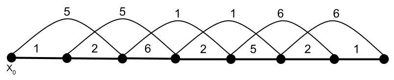
Figure 12: A demonstration of the transition described in Lemma 15 with $n^{\prime}=1$, $b^{\prime}=2$. Note that on the left side of the figure, we follow protocol $(x_{0},\{0\mapsto 5,1\mapsto 5\})$, while on the the right, we follow protocol $(x_{0},\{0\mapsto 6,1\mapsto 6\})$. Here the $k$ from the lemma would be $0$.

Figure 12 shows the technique used in Lemma 15. Now we can establish Lemma 14:

Proof.

Of course it suffices to consider the case where $c$ and $c^{\prime}$ differ in exactly two entries, say at $r_{1},r_{2}\in\mathbb{Z}/b^{\prime}$.

We first find a sequence $k_{0},\ldots,k_{l}\in\mathbb{Z}/(2b^{\prime})$ with the following properties:

1. The $k_{i}$’s are distinct mod $b^{\prime}$.

2. $\{k_{0},k_{l}\}=\{r_{1},r_{2}\}$ (mod $b^{\prime}$).

3. $k_{i+1}=k_{i}+n^{\prime}$ (mod $2b^{\prime}$) for each $i$.

4. $\overline{c}(k_{0})=\overline{c}(k_{l})$ if and only if $l$ is odd.

To do so, first consider the sequence $j_{0},\ldots,j_{b^{\prime}}\in\mathbb{Z}/(2b^{\prime})$ defined by $j_{i}=r_{1}+in^{\prime}$. Since $n^{\prime}$ is coprime to $b^{\prime}$, there must be some $0<i_{0}<b^{\prime}$ such that $j_{i_{0}}=r_{2}$ (mod $b^{\prime}$). Our sequence of $k_{i}$’s will either be the sequence $j_{0},\ldots,j_{i_{0}}$ or the sequence $j_{i_{0}},\ldots,j_{b^{\prime}}$. In either case, conditions $2$ and $3$ will hold by construction, and condition 1 will hold since $n^{\prime}$ is coprime to $b^{\prime}$.

For condition 4, we use the fact that $j_{b^{\prime}}=j_{0}+b^{\prime}$ (mod $2b^{\prime}$), and so $\overline{c}(j_{b^{\prime}})=\neg\overline{c}(j_{0})$. Thus, whatever the value of $\overline{c}(j_{i_{0}})$, one of our two options above will give $\overline{c}(k_{0})=\overline{c}(k_{l})$ and the other will give $\overline{c}(k_{0})=\neg\overline{c}(k_{l})$. Since $b^{\prime}$ is even, $i_{0}$ and $b^{\prime}-i_{0}$ have the same parity, so one of these options will give us condition 4.

Now, by Lemma 15, we can change the colors $c(k_{i})$ and $c(k_{i+1})$ for some adjacent pair of elements $k_{i}$ and $k_{i+1}$ in our sequence if they are assigned the same value by our double code. This is exactly the type of move we are allowed to make in the game from Lemma 13, though. Condition 4 is exactly the hypothesis from that lemma, so we can find a sequence of moves which change the code entry at $k_{0}$ and $k_{l}$, but nowhere else. By condition 2, this is exactly what we wanted. ∎

We now return to our original situation with $\Gamma=\mathbb{Z}/2\times\mathbb{Z}$. Recall that we have fixed a generator $(0,b)\in S^{\prime}$ with $b$ even. Let $q=\gcd(b,n)$, and let $b^{\prime}=b/q$ and $n^{\prime}=n/q$. Also let $b^{\prime\prime}$ be the largest power of 2 dividing $b^{\prime}$ (equivalently $b$).

If $b^{\prime\prime}\mid m$, then by working separately on each $\mathbb{Z}/2\times b^{\prime\prime}\mathbb{Z}$-orbit, we can treat the $(0,b)$ as $(0,b/b^{\prime\prime})$, and since $b/b^{\prime\prime}$ is odd, we know already how to handle these. Thus assume $b^{\prime\prime}\not|\ m$. Further assume $m\in(0,b^{\prime\prime})$ (mod $2b^{\prime\prime}$), as the argument in the case $m\in(b^{\prime\prime},2b^{\prime\prime})$ (mod $2b^{\prime\prime}$) will be similar.

Let $c:\mathbb{Z}/b^{\prime\prime}\rightarrow\{5,6\}$ a code. We will say a coloring of the $(0,b)$-edges follows protocol $(x_{0},c)$ if the edge $((\epsilon,k)\cdot x_{0},(\epsilon,k+b)\cdot x_{0})$ gets the color $\overline{c}(k)$ for each $(\epsilon,k)\in\Gamma$. Observe that this does describe a valid edge coloring since $b/b^{\prime\prime}$ is odd.

Let $c_{0}:\mathbb{Z}/b^{\prime\prime}\rightarrow\{5,6\}$ be the code taking the constant value 5. It suffices to be able to transition between the protocols $(x_{0},c_{0})$ and $((0,1)\cdot x_{0},c_{0})$, or equivalently $(x_{0},c_{0}^{\prime})$, where $c_{0}^{\prime}(0)=6$ but $c_{0}^{\prime}=5$ everywhere else. An example of the protocol $(x_{0},c_{0})$ is shown in part (a) of Figure 13.

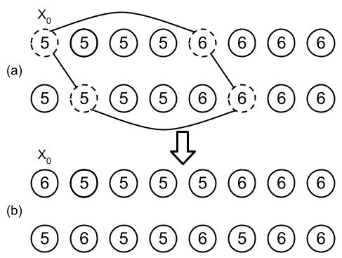
Figure 13: A demonstration of step 1 in the procedure for the $(0,b)$-edges when $b=b^{\prime}=b^{\prime\prime}=4$ and $m=1$, in the style of Figure 10. As in that figure, the label of a vertex $x$ denotes the color of the edge $(x,(0,b)\cdot x)$. (a): A coloring following protocol $(x_{0},c_{0})$ for the $(0,b)$-edges, along with the setup for step 1. The dashed vertices are those included in one of the $(0,b)$-orbits along which parity is changed. The edges drawn are the $(0,b)$ and $(1,m)$-edges involved in making that change for these orbits. (b): The effects of step 1. Observe that in the orbit $\mathbb{Z}\cdot x_{0}$, the $(0,b)$-edges now follow protocol $((0,1)\cdot x_{0},c_{0})$.

Our procedure for this transition will occur in two steps. Step 1 is pictured in Figure 13. In it, once again following the procedure from Subsubsection 4.3.1, we use the $(1,m)$ edges to swap parity along certain pairs $f,(1,m)\cdot f$ of $(0,b)$-orbits. Specifically, we will do this for each $f$ containing a point of the form $(0,kb^{\prime\prime})\cdot x_{0}$. Note that here the condition $m<b^{\prime\prime}$ (mod $2b^{\prime\prime}$) is used to get condition 3 from Lemma 4.

The result of this step is shown in part (b) of the figure. It should be clear that, after making, it, the $(0,b)$-edges in the orbit $\mathbb{Z}\cdot x_{0}$ follow our desired protocol $(x_{0},c_{0}^{\prime})$, but not those in the orbit $(\mathbb{Z}+(1,0))\cdot x_{0}$. Instead, on this orbit, the $(0,b)$-edges follow the protocol $(x_{0},c_{0}^{\prime\prime})$, where $c_{0}^{\prime\prime}(m)=6$, but $c_{0}^{\prime\prime}=5$ everywhere else. In particular, since $m\neq 0$ (mod $b^{\prime\prime}$), $c_{0}^{\prime\prime}$ and our desired code $c_{0}^{\prime}$ differ in exactly 2 places. (And their corresponding double codes differ in 4 places.)

For step 2, within this second $\mathbb{Z}$-orbit, we will work separately within each $q\mathbb{Z}$-orbit to correct this. Fix some such orbit $q\mathbb{Z}\cdot x_{0}^{\prime}$, where $x_{0}^{\prime}=(1,r)\cdot x_{0}$ for some $0\leq r<q$. Within this orbit, the generators $(0,b)$ and $(0,n)$ behave like $b^{\prime}$ and $n^{\prime}$, and these satisfy the hypotheses used for the $b^{\prime}$ and $n^{\prime}$ from the setting of Lemma 14.

Using the terminology from that setting, let $c$ be the code of our coloring for this orbit relative to $x_{0}^{\prime}$ following step 1, and $c^{\prime}$ the code relative to $x_{0}^{\prime}$ that we want to transition to.

For the sake of clarity, we remark that these are codes with domain $\mathbb{Z}/b^{\prime}$, while the codes $c_{0}^{\prime\prime}$ and $c_{0}^{\prime}$ have domain $\mathbb{Z}/b^{\prime\prime}$. While this is an important difference to keep in mind, what follows will still make sense since $b^{\prime\prime}$ is an odd multiple of $b^{\prime}$.

Then, the corresponding double code $\overline{c}$ is given by $\overline{c}(k)=\overline{c_{0}^{\prime\prime}}(r+kq)$, and likewise for $\overline{c^{\prime}}$ and $\overline{c_{0}^{\prime}}$. Now $q$ is coprime to $2b^{\prime\prime}$ since the former is odd and the latter is a power of 2. Therefore, as $k$ ranges over $\mathbb{Z}/(2b^{\prime})$, $r+kq$ will take every value mod $2b^{\prime\prime}$ $b^{\prime}/b^{\prime\prime}$ times. Therefore, since $\overline{c_{0}^{\prime}}$ and $\overline{c_{0}^{\prime\prime}}$ differ in 4 places, $\overline{c^{\prime}}$ and $\overline{c}$ differ in $4b^{\prime}/b^{\prime\prime}$ places, and so $c^{\prime}$ and $c$ differ in $2b^{\prime}/b^{\prime\prime}$ places. This is even, so by Lemma 14 a transition is possible, and we are done.

This was the last type of generator we had to deal with, so we can record our result:

Lemma 16.

If $(1,0)\notin S$, $\chi_{B}^{\prime}(\Gamma,S)=|S|$.

Of course, Lemmas 11 and 16 together complete our proof of statement 2 of Theorem 2, and hence of Theorem 2. ∎

References

- [1] F. Bencs, A. Hrušková, and L.M. Tóth, Factor of iid Schreier decoration of transitive graphs.
- [2] C. Conley, S. Jackson, A. Marks, B. Seward, and R. Tucker-Drob, Borel asymptotic dimension and hyperfinite equivalence relations. https://arxiv.org/pdf/2009.06721.pdf
- [3] C.T. Conley and B.D. Miller, A bound on measurable chromatic numbers of locally finite Borel graphs, Math. Res. Lett., 23 (2016), no. 6, 1633-1644.
- [4] S. Gao, S. Jackson, E. Krohne, and B. Seward, Borel combinatorics of abelian group actions. in preparation.
- [5] J. Grebík, O. Pikhurko, Measurable Versions of Vizing’s Theorem. Adv. Math 374 (2020).
- [6] J. Grebík, V. Rozhoň, Of toasts and tails. https://arxiv.org/pdf/2103.08394.pdf
- [7] S. Jackson, A.S. Kechris and A. Louveau, Countable Borel equivalence relations. J. Math. Logic, 2 (2002), 1-80.
- [8] A.S Kechris and A.S. Marks, Descriptive graph combinatorics, preprint, 2019; posted in http://www.math.caltech.edu/kechris/
- [9] A.S. Kechris, S. Solecki, and S. Todorcevic, Borel chromatic numbers, Adv. Math., 141 (1999), 1-44.
- [10] A. Marks, A determinacy approach to Borel combinatorics. J. Amer. Math. Soc. 29 (2016), 579-600.
- [11] B.D. Miller, Ends of graphed equivalence relations, I, Israel J. Math., 169(1) (2009), 375–392.
- [12] L.M. Tóth, Invariant Schreier decorations of unimodular random networks. https://arxiv.org/abs/1906.03137
- [13] F. Weilacher, Borel Vizing’ theorem for 2-ended groups. https://arxiv.org/abs/2101.12740