Metallic nanostructures as electronic billiards for nonlinear terahertz photonics

Abstract

The optical properties of metallic nanoparticles are most often considered in terms of plasmons, the coupled states of light and quasi-free electrons. Confinement of electrons inside the nanostructure leads to another, very different type of resonances. We demonstrate that these confinement-induced resonances typically join into a single composite ”super-resonance,” located at significantly lower frequencies than the plasmonic resonance. This super-resonance influences the optical properties in the low-frequency range, in particular, producing giant nonlinearities. We show that such nonlinearities can be used for efficient down-conversion from optical to terahertz and mid-infrared frequencies on the sub-micrometer propagation distances in nanocomposites. We discuss the interaction of the quantum-confinement-induced super-resonance with the conventional plasmonic ones, as well as the unusual quantum level statistics, adapting here the paradigms of the quantum billiard theory and showing the possibility to control the resonance position and width using the geometry of the nanostructures.

Introduction. Light propagating in the vicinity of metallic surfaces or metallic nanostructures is strongly coupled to the “electronic fluid” formed by quasi-free electrons in the metal, resulting in joint electron-photon excitations which are called surface or particle plasmons, depending on the geometry. Plasmons, and the corresponding plasmonic resonance (PR) are at the very heart of optics of nanostructures.

PRs appear by matching of the incoming light to the intra-particle fields, leading to strong surface charges and resonance peaks of linear and nonlinear response of metallic nanoparticles at certain frequencies Mie (1908); Kreibig and Vollmer (2013); Kim et al. (2010). That is, PRs are defined via the matching condition of the fields, rather than electrons themselves, and have no direct relation to the electron confinement inside the nanostructure. Plasmonic resonances are located at quite high frequencies, commonly in the visible range.

As soon as we consider very small metallic nanoparticles, quantum confinement of electrons in the finite volume of a nanoparticle comes into play. Possible confined-based resonances have rarely attracted attention per se, separately from the properties of plasmons. On the other hand, any calculation of the properties of small nanoparticles does in principle include quantum mechanical confinement of electrons as an ingredient, noticeably influencing the position and the width of PR Kawabata and Kubo (1966); Ruppin and Yatom (1976); Kraus and Schatz (1983); Kreibig and Vollmer (2013); Amendola et al. (2017). In the recent years, huge progress was made in both calculations and measurements Scholl et al. (2012); Morton et al. (2011); Philip et al. (2012); Kreibig and Vollmer (2013); Boyd et al. (2014); Qian et al. (2016); Amendola et al. (2017); Varas et al. (2016); Zhou et al. (2021) of properties of small nanoparticles. Theoretical approaches, starting from relatively simple analytical techniques Wood and Ashcroft (1982); Hache et al. (1986); Sato et al. (2015); Kawabata and Kubo (1966), through the single-electron-in-box Wood and Ashcroft (1982); Genzel et al. (1975), jellium model Brack (1993), hydrodynamic-like equations Ginzburg et al. (2014); Hurst et al. (2014) and quantum hydrodynamic theory Takeuchi and Yabana (2022) towards direct ab-initio DFT methods fully taking into account the ionic core structure Morton et al. (2011); Zhang et al. (2017); Zhou et al. (2021); Barbry et al. (2015); Rossi et al. (2017) are used; for a review see Varas et al. (2016). Whereas analytical and hydrodynamic approaches can address nonlinear properties Hache et al. (1986); Ginzburg et al. (2014); Hurst et al. (2014), complex ab-initio methods focus solely on the linear susceptibility, unless very small nanoclusters are considered Day et al. (2010, 2016).

For very small nanoclusters and nanoparticles (few hundreds of atoms and below), the response is molecular-like Morton et al. (2011); Zhou et al. (2021), typically including a cacophony of resonances replaced by a single PR Zhou et al. (2016, 2021); Townsend and Bryant (2012). At lower frequencies, a prominent molecular-like resonance is the HOMO-LUMO transition Barcaro et al. (2006); Kwak et al. (2017); Zhou et al. (2019, 2021). It describes an excitation of a single localized electron, and depends heavily on the molecular structure Barcaro et al. (2006).

As we shift to larger nanoparticles, the HOMO-LUMO transition effectively fades out Zhou et al. (2021) because its decay rate grows exponentially with the size of the nanostructure Kwak et al. (2017); Zhou et al. (2019). However, the PR is not the only one which remains. Signatures of a single resonance well below the plasmonic one but above the HOMO-LUMO transition were observed experimentally Oates and Mücklich (2005); Wyrwas et al. (2007) and later confirmed theoretically Scholl et al. (2012); He and Zeng (2010) involving ab-initio simulations He and Zeng (2010). This resonance is however mostly overlooked since then, and there is no consensus in explanations of its nature. Whereas in Scholl et al. (2012); Wyrwas et al. (2007) the confinement-based argument were put forward, Oates and Mücklich (2005); He and Zeng (2010) tries to explain it without leaving the plasmonic framework by introducing ”restoring force on the electrons”.

Here we show that confinement-based resonances under normal conditions (at least for nanostructures with regular enough geometry) merge together and form a single broadband “super-resonance” located commonly in THz and MIR frequency range, with both the width and position widely controllable with the nanostructure geometry. Such super-resonance must be considered as one of the universal signatures of metallic nanostructures, yet fundamentally different from the PR.

We study the statistical features of confinement-based resonances by adapting and modifying the paradigm of neighboring-level statistics from the field of quantum billiards Stöckmann (1999). Electrons confined in a nanostructure certainly represents a type of quantum billiard. Yet, up to now, with only very few exceptions Simons and Altshuler (1993); Ravnik et al. (2021), non-metallic billiards such as semiconductor quantum dots Nakamura and Thomas (1988); Jalabert et al. (1990); Akis et al. (1997); Zozoulenko and Berggren (1997); Burke et al. (2010); Ponomarenko et al. (2008); Kuchařík et al. (2019) were considered. As we show, the metallic nature of our billiard provides an unique opportunity to observe certain features the level statistics directly in the optical properties.

Furthermore, the super-resonance provides a broadband nonlinear response, leading to giant nonlinearities. We demonstrate how these nonlinearities can be used for an efficient optical rectification and difference-frequency mixing in the nanocomposites, enabling broadband conversion from optical to MIR or THz ranges by sub-micrometer devices.

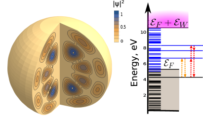
Figure 1: A spherical gold nanostructure (left) of 2.75 nm diameter and the band level structure (right) appearing due to the electron confinement (quantum billiard resonances). Fermi energy $\mathcal{E}_{F}$ and work function $\mathcal{E}_{W}$ as well as exemplary virtual transitions contributing to linear (orange arrows) and nonlinear (red arrows) properties are indicated. One of the wavefunctions $\psi(x,y,z)$ is visualized inside the nanostructure (a sector of the sphere is cut for visualization purposes). Even for the simplest nanoparticles, energy level structure is quite complex.

The model. We used a simple analytical approach of a single-particle-in-a-box Kraus and Schatz (1983); Hache et al. (1986); Wyrwas et al. (2007); Scholl et al. (2012) (see also more details in Supplementary) with electron fully confined inside a nanoparticle. For calculation of optical properties, we consider electron energy structure characterized by Fermi energy $\mathcal{E}_{F}$ and work function of $\mathcal{E}_{W}$, as illustrated in Fig. 1 right. This approximation works well for metals with a simple Fermi surface such as alkali metals (Li, Na, Ca, Rb), it is an acceptable simplification for metals with somewhat more complicated Fermi surfaces such as Cs, Cu, Ag or Au, and is barely applicable at all for other metals. The linear ($\chi^{(1)}$) and nonlinear ($\chi^{(3)}$) susceptibilities were calculated using a version of the standard perturbative iterative approach Boyd and Prato (2008) which takes into account selection rules following from the Fermi-Dirac statistics (see Supplementary). The linear and nonlinear optical properties can be described via a sum of contributions of virtual transitions from inside the Fermi sea to outside and back [see orange (linear) and red (nonlinear) arrows Fig. 1]. We also assumed fast population decay time $T_{1}=50$ fs and dephasing time $T_{2}=5$ fs Hache et al. (1986).

To be more specific, in our numerical simulations we consider gold since it is a very widespread material, and is suitable for composites due to low imaginary part of susceptibility. Yet we note that conclusions we draw below are basically metal-independent (taking into account precautions mentioned above). In gold, a simple ideal-metal picture discussed above neglects several linear and nonlinear effects, such as interband transitions, influence of finite temperature, and hot-electron nonlinearities. However, these effects are negligible for low-frequency response in THz or MIR range driven by femtosecond pulses, and our model remains adequate in this regime (see Supplementary for justifications and detailed estimates).

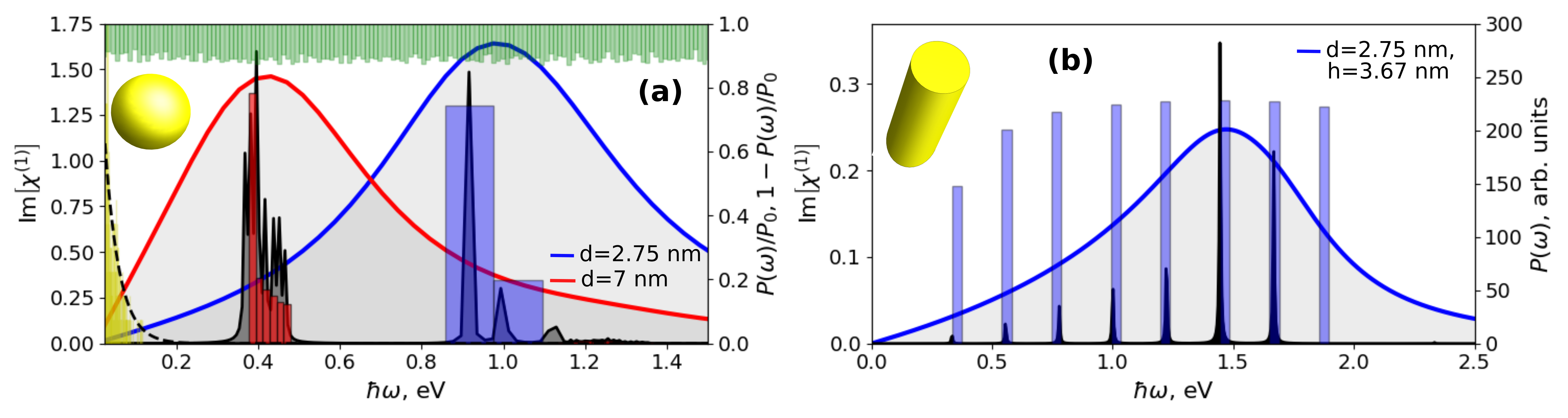
Figure 2: Billiard resonances and weighted level statistics for a golden sphere of few exemplary diameters $d$ (a) and a cylinder (b) of the diameter $d$ and height $h$. The blue and red curves in (a) and (b) show $\operatorname{Im}{(\chi^{(1)})}$ as the function of frequency for different sizes (see legend). Bars of the same colors show the corresponding weighted level statistics $P(\omega)$ normalized to some $P_{0}$ ($P_{0}$ is not the same for different curves). Green bars show the statistics for all allowed transitions attached, for visibility, to the upper $x$-axis (that is, technically, $1-P(\omega)/P_{0}$ is shown; see also larger frequency scales in Supplementary). Black lines show $\operatorname{Im}{(\chi^{(1)})}$ for $T_{2}$ increased 100 times. Yellow bars show NLS and dashed black line indicates the Poissonian statistics.

Quantum billiard (confinement-based) resonances. The typical level structure obtained by the above model for an exemplary spherical gold nanoparticle of the diameter $d=2.75$ nm is shown in Fig. 1. These levels originate from electron confinement in the nanostructure. Even in the presented case of a very simple particle, the levels look quite irregular. This is a familiar picture in the framework of of quantum billiard theory Stöckmann (1999), were the statistical properties of the level distribution play one of the central roles. For instance, one can consider the neighboring level statistics (NLS), which allows to distinguish between integrable (regular) and non-integrable (chaotic) billiards. For the regular billiards, such as spheres, the probability density $P(\omega)$ of neighboring-level distance $\omega$ obeys Poissonian statistics: $\ln{P(\omega)}\propto-\omega$. This is also true in our case: NLS corresponding to Fig. 1 is plotted in Fig. 5(a) by yellow bars and coincides well with the Poissonian distribution (black dashed line).

Judging from such statistics, one might expect a conglomerate of resonances near zero frequency, but this is not the case. An optical response $\chi^{(1)}$ resulting from the electron confinement for few exemplary nanostructures is shown in Fig. 5. Note that, in addition to the confinement-based impact shown in Fig. 5, the full linear response includes also the so-called Drude part, representing the action of quasi-free-electrons (see Supplementary for more details).

The clearly observed feature of the confinement-based linear response is the presence of a single resonance-like peak in the IR/THz range at a non-zero resonance frequency $\omega_{\mathrm{conf}}$ which quickly decreases with increasing particle size. Such peak was observed experimentally Oates and Mücklich (2005); Wyrwas et al. (2007) and theoretically Scholl et al. (2012); He and Zeng (2010). It is easy to see that this resonance coincides well with the minimally possible allowed transitions close to the Fermi energy which can be, for a spherical nanoparticle, analytically estimated as (see Supplementary for details), cf. also Wyrwas et al. (2007)):

$$\omega_{\mathrm{conf}}\approx\frac{\pi}{r}\sqrt{\frac{\mathcal{E}_{F}}{2m_{e}}},$$ (1)

where $m_{e}$ is the electron mass. This makes it fundamentally different from the PR, being located at a significantly lower frequency. Yet, why does only a single resonance arise? Can we influence it width and position? These and related questions will be addressed in the following paragraphs.

Closer consideration allows to establish that, starting already from quite small nanosphere diameters $d\approx 2.5$ nm, the resonance near $\omega_{\mathrm{conf}}$ is composed of many transitions with nearby frequencies [see Fig. 5(a)]. These transitions merge into one single “super-resonance”. This is especially well observable if we consider much larger $T_{2}$ (which would correspond to low temperatures Kabanov and Alexandrov (2008)). In this case, many separated resonances are indeed visible in the optical response, as shown in Fig. 2(a,b) by black curves. The particular structure of the transitions depends significantly on the geometry [cf. Fig. 5(b) for a cylinder]. For instance, the position and width of the super-resonance for a cylinder are shifted in comparison to a sphere with the same volume and diameter by the noticeable amount of 35% and 23%, correspondingly. Nevertheless, Eq. 1 remains a valid, yet rough estimation of the position of the resonance.

Both the position of the super-resonance $\omega_{\mathrm{conf}}$ and its structure can be analyzed using the level-distance statistics similar to NLS. A naïve approach would be to calculate such statistics using all dipole-allowed transitions between the confinement-based levels, shown in downward green rectangles in Fig. 2(a), and covering extremely broad range around 10 eV (see green bars in Fig. 2(a) and also Supplementary). However, it must be modified to include only transitions from below to above of $\mathcal{E}_{F}$, obviously corresponding to the Pauli principle and absence of population above the Fermi level. In addition, in the statistics we weight the transitions by the square of the corresponding dipole momentum, thus taking into account the known tendency of the transition dipole momenta to rapidly decrease, on average, with the energy difference. The resulting modified statistics is shown by the red and blue bars in Fig. 5 and agrees nicely (for large $T_{2}$) both with the position of the super-resonance and with its width for small $T_{2}$. The super-resonance has a certain “natural” width, for the case of nanospheres it can be estimated as $\omega_{\mathrm{conf}}/4$ (see Supplementary). Analysis of the position of the super-resonance for nanospheres (see Supplementary) indicates that the energy of the participating states is located mostly in radial (rather than angular) motion.

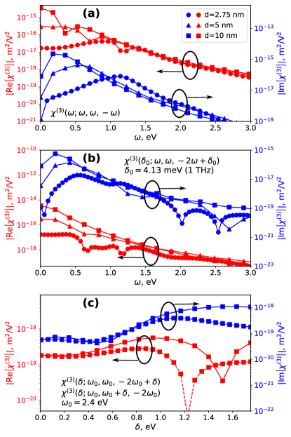
Figure 3: Nonlinear susceptibility for the Kerr nonlinearity (a) and for different FWM processes leading to the optical rectification (b,c) in dependence on the signal $\delta$ (c) and pump $\omega$ (b) frequency, shown for the nanostructures of different diameters.

Nonlinearities. The above described low-frequency resonance is expected to lead also to strong nonlinearities; in our case, $\chi^{(3)}\neq 0$ as calculated using the approach described above. We note that such approach to calculate Kerr nonlinearity was already utilized in Hache et al. (1986), however, instead of discrete spectrum, approximation of continuous density of states was used. Nevertheless, we checked that our calculations are in quantitative agreement with Hache et al. (1986); they are also in agreement with experimental measurements for short pulses (see Boyd et al. (2014) and references therein). An example of $\chi^{(3)}(\omega;\omega,\omega,-\omega)$ for the four-wave-mixing (FWM) process $\omega+\omega-\omega=\omega$ (corresponding to the Kerr nonlinearity) is shown in Fig. 3(a) for several diameters. The low-frequency resonance we observed in $\chi^{(1)}$ is also well-visible here. Whereas in the linear response the Drude part dominates (see Supplementary), in the nonlinear response it is fully absent.

We now try to exploit this low-frequency resonance. Motivated by detection and spectroscopic applications of THz and MIR radiation, we focus on the FWM providing a signal in THz and MIR range, generated from a sub-100 fs pump pulse. Nonlinear susceptibilities $\chi^{(3)}(\delta;\omega,\omega,-2\omega+\delta)$ and $\chi^{(3)}(\delta;\omega,\omega+\delta,-2\omega)$, leading to generation of low-frequency signal at frequency $\delta$ as a result of a FWM process in a two-color pump at frequencies $\omega$ (fundamental) and $2\omega$ (its second harmonics) are presented in Fig. 3(b-c). Both Kerr rectification nonlinearities presented in Fig. 3 are several orders of magnitude higher than the Kerr nonlinearity of the fused silica $\sim 2\times 10^{-22}$ m²/V². In Fig. 3(a), where pump-frequency dependencies are shown, the billiard super-resonance described above is very clearly visible. This is not a unique property of metallic nanostructures. Giant nonlinearities in semiconductor nanostructures due to billiard resonances were recently predicted in Kuchařík and Němec (2021).

Efficient frequency difference generation. As an interesting application we consider the process of optical rectification and difference frequency generation, governed by three nonlinearities $\chi^{(3)}(\delta;\omega_{0},\omega_{0},-2\omega_{0}+\delta)$, $\chi^{(3)}(\delta;\omega_{0}+\delta,\omega_{0},-2\omega_{0})$ and $\chi^{(3)}(\delta;\omega_{0},\omega_{0}+\delta,-2\omega_{0})$, with a two-color optical pump at around $\omega_{0}$ and $2\omega_{0}$ and signal $\delta\ll\omega_{0}$ in THz and MIR. We solve the propagation equations, assuming slowly varying envelope approximation and taking into account dispersion relations, but neglecting nonlinear effects for the pump waves because of very very small propagation distance (see Supplementary for details). Both $\chi^{(3)}_{\mathrm{eff}}$ and the linear susceptibility $\chi^{(1)}_{\mathrm{eff}}$ are calculated from given linear and nonlinear properties of the nanoparticles ($\chi^{(1)}_{\mathrm{NP}}$, $\chi^{(3)}_{\mathrm{NP}}$) and host ($\chi^{(1)}_{\mathrm{h}}$, $\chi^{(3)}_{\mathrm{h}}$) using the effective medium approach Zeng et al. (1988) (see Supplementary). By calculation of the linear properties the full linear susceptibility containing both confinement-based and Drude parts are included. As a host material, we take fused silica which possesses strong losses in the range between 30 and 40 THz (see Fig. 4), but otherwise is quite transparent Palik (1998). We consider the filling factor of $f=0.01$ and neglect the nonlinearity of the host. Resulting effective linear quantities are shown in Fig. 4 and demonstrate the usual PR resonance at around 2.4 eV with the width of around 30 THz. The shortest pulses still supported by this resonance are around 30 fs in duration.

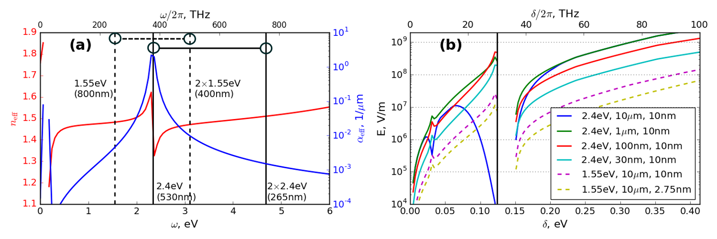
Figure 4: Efficient generation of THz and MIR light in a composite of gold spheres with 2-color pump. (a) effective refractive index $n_{\mathrm{eff}}$ and effective losses $\alpha_{\mathrm{eff}}$ in dependence on frequency $\omega$ for a gold nanostructures with $r=10$ nm immersed into fused silica ($f=0.01$). Vertical lines show two variants of the 2-color pump at $\omega_{0}=1.55$ eV ($\lambda_{0}=530$ nm, dashed line) and $\omega_{0}=2.4$ eV ($\lambda_{0}=530$ nm, solid line). The horizontal lines connect the spectral components of two-color pump. (b) The generated field amplitude for different propagation distances $L$ and nanostructure diameter $d$ (see legend) and the pump as described in text. Solid vertical line in (b) separates THz from MIR band.

Assuming an exemplary pulse durations of around 30 fs, we must consider two regions for the pump where conversion works significantly different. For the signal in the THz range ($\delta/2\pi\leq$ 30 THz), the frequencies $j\omega_{0}$ and $j\omega_{0}+\delta$ ($j=1,2$) are both located within the spectrum of the pump. In contrast, for the signal in MIR range $\delta/2\pi>$ 30 THz, the components $\omega_{0}+\delta$, $2\omega_{0}+\delta$ are not within the pump spectrum anymore. This leads to different treatment of these two frequency ranges for the selected pulse duration (see Supplementary).

The resulting field amplitude at 0th harmonic $A_{0}$ is given in Fig. 4(b) for different parameters and for the pump amplitudes $A_{1}=A_{2}=10^{10}$ V/m. This pump for 30-fs pulses corresponds to a fluence around 0.3 J/cm², which is yet below the damage threshold of gold (around 0.5 J/cm² Poole et al. (2013)) and of fused silica (around 1 J/cm² Chimier et al. (2011)). One can see that in THz range the signal amplitude reaches $5\times 10^{8}$ V/m corresponding to efficiency of around $10^{-3}$. In MIR range, the amplitude can exceed $10^{9}$ V/m, delivering efficiencies above the percent level. Moreover, the maximal efficiency is achieved at 100 nm propagation distance for THz signal and 1 $\mu$m for MIR signal. From Fig. 4(b) one can also see that the most efficient conversion is achieved for the pump frequency $\omega_{0}$ centered at the PR (solid lines in Fig. 4). In this case, the coupling of the pump to the signal is most efficient.

Discussion and conclusions. We showed that confinement-based energy levels in metallic nanostructures, representing an integrable (or close to integrable) quantum billiards, typically join together into a single ”super-resonance”, which position and width can be controlled by the geometry of the nanostructure. Whereas we focused here on (almost) integrable quantum metallic billiards, we anticipate richer resonance structure and control possibilities if truly chaotic billiards are considered. We analyzed the super-resonance, using the level statistics extended in comparison to typically used in quantum chaos theory. In the linear regime the ballistic super-resonances is ”hidden” behind the much stronger Drude response, yet it manifests itself strongly in a giant nonlinearity. This nonlinearity can be in addition enhanced by interaction with plasmons and effectively used to down-convert light to THz and MIR range with high efficiency already after 100-nm distances, despite of huge linear and nonlinear losses. Our confinement-based framework might also be helpful in a deeper understanding of the recent experimental work on efficient THz generation in nanostructures Luo et al. (2014); Keren-Zur et al. (2019) and paves a way to extend newly proposed electronic meta-devices Samizadeh Nikoo and Matioli (2023) into the nonlinear regime.

I Supplementary

I.1 Simplified Hamiltonian and wavefunctions for the case of spherical particles

To approach the problem analytically, we consider a spherical metallic particle of the radius $a$ (diameter $d=2a$). Since we are interested in low frequencies, we neglect the interband transitions. We neglect the temperature effects assuming that $N$ electrons in conduction band occupy all levels below Fermi energy $\mathcal{E}_{F}$ (see Fig. 1 of the main article). The energy structure is calculated assuming one-electron approximation and corresponds to that of a single free electron in a infinite-strength spherical potential of the radius $a$. To take into account finiteness of the potential, the levels above the work function $\mathcal{E}_{W}$ are disregarded. The validity of these approximations is justified below.

The corresponding single-particle eigenproblem can be then formulated as $\hat{H}_{0}\psi=\mathcal{E}\psi$, with $H_{0}=-\hbar^{2}/2m_{e}\Delta+V(r)$, $V(r)=0$ for $r\leq a$ and $V(r)=\infty$ for $r>a$ ($m_{e}$ is the electron mass). With the approximations above, we neglect various effects of electron-electron and electron-ion interaction such as interband transitions, electron heating, the change of the eigenstates due to the finite height of the potential, and other effects, which play only minor role at low frequencies and ultrashort sub-100-fs pulse durations. The validity of this approximation is discussed in Sec. I.6 below. As it will be shown there, our simple model is rather adequate for the parameters we consider, despite of its simplicity. The advantage of this approach is the possibility to determine the energy structure analytically. The corresponding eigenfunctions are combinations of spherical harmonics. The energies are defined as

$$\mathcal{E}_{nl}=\mathcal{E}_{0}\alpha_{nl}^{2}$$ (2)

where $n,l$ are quantum numbers,

$$\mathcal{E}_{0}=\dfrac{\hbar^{2}}{2m_{e}a^{2}},$$ (3)

and $\alpha_{nl}$ is the $n$th zero of the Bessel function of order $l$. In contrast to the Coulomb potential, there is no degeneracy in $l$.

The eigenfunctions of the problem described in the main article are:

$$\psi_{nlm}(r,\theta,\phi)=R_{nl}(r)Y_{l}^{m}(\theta,\phi),$$ (4)

where $n,m,l$ are quantum numbers, $R_{nl}(r)=\dfrac{\sqrt{2}j_{l}(\alpha_{nl}r/a)}{\sqrt{a^{3}}j_{l+1}(\alpha_{nl})}$, $Y_{l}^{m}$ are spherical functions ($-l\leq m\leq l$), $j_{l}$ is the spherical Bessel function of order $l$, and $\alpha_{nl}$ is its $l$th zero.

The radial part of the matrix element is, for the allowed transitions $l^{\prime}-l=\pm 1$,

$$\mu_{nl,n^{\prime}l^{\prime}}=\frac{4ae\mathcal{E}_{0}\sqrt{\mathcal{E}_{nl}\mathcal{E}_{n^{\prime}l^{\prime}}}}{(\mathcal{E}_{n^{\prime}l^{\prime}}-\mathcal{E}_{nl})^{2}},$$ (5)

and zero in other cases (here $e$ is the electron charge).

I.2 Cylindrical geometry

In this section we determine the eigenvalues for the cylindrical geometry. We assume here that the main axis of the cylinder oriented along $z$-direction, and the light is assumed to be linearly polarized also in $z$-direction. Note the difference in the denotations with the part where propagation is considered: there, $z$-direction is the direction of the light propagation.

The eigenfunctions in $(r,\theta,z)$-coordinates are Okamoto (2021):

$$\psi_{nlm}(r,\theta,z)=C_{nlm}J_{m}(r\tilde{\alpha}_{lm}/a)\cos(m\theta)\cos(\pi nz/h),$$ (6)

where $C_{nlm}$ is the normalization factor, $h$ is the height of the cylinder, $\tilde{\alpha}_{lm}$ is $l$th zero of the Bessel function $J_{m}(x)$ of order $m$. These eigenfunctions are described by three integer quantum numbers: $n$ describes the localization in $z$ direction, $m$ and $l$ – along the orthogonal directions.

The energies of these eigenstates are given by the expression

$$\mathcal{E}_{nlm}=\frac{\hbar^{2}}{2m_{e}}\left(\frac{\tilde{\alpha}_{lm}^{2}}{a^{2}}+\frac{4\pi^{2}n^{2}}{h^{2}}\right).$$ (7)

Because the light is assumed to be linearly polarized in $z$-direction, only $z$-components of the dipole moments

$$\mu_{nlm,n^{\prime}l^{\prime}m^{\prime}}=\left\langle\psi_{nlm}\right|z\left|\psi_{n^{\prime}l^{\prime}m^{\prime}}\right\rangle$$ (8)

play a role, and they can be calculated as:

$$\mu_{nlm,n^{\prime}l^{\prime}m^{\prime}}\propto\frac{2nn^{\prime}\left((-1)^{n+n^{\prime}}-1\right)}{(n-n^{\prime})^{2}(n+n^{\prime})^{2}}\delta_{ll^{\prime}}\delta_{mm^{\prime}},$$ (9)

where we omitted for simplicity a pre-factor which comes from the normalization of the wavefunctions.

I.3 Derivation of Eq. 1 of the main article

As we see in the main article (see also below), the main role in the super-resonance is played by the transitions close to the Fermi energy $\mathcal{E}_{F}$. For not very small nanostructures, this corresponds to relatively large $l$ and $n$. For large $n$ and $l$ an analytical estimation

$$\alpha_{nl}\approx(2n+l)\pi/2$$ (10)

is possible. Based on this, the energy difference between the allowed transitions $\Delta l=\pm 1$ near the energy $\mathcal{E}$ is

$$\Delta\mathcal{E}=\pi\sqrt{\mathcal{E}\mathcal{E}_{0}}.$$ (11)

Near the Fermi energy $\mathcal{E}\approx\mathcal{E}_{F}$, substituting Eq. (3), we obtain Eq. 1 of the main article, with $\hbar\omega_{\mathrm{conf}}$ identical to $\Delta\mathcal{E}$.

We note that Eq. (10) is valid for $n\gg l$. In contrast, for $n\approx 1$ we have $\alpha_{nl}\approx(2n+l)$, that is, the positions of the resonances would be shifted in this latter case by the factor $\sim\pi/2$ to the lower frequencies. The resonances shown in Fig. 2 of the main article as well as in Fig. 5 coincide well with Eq. (10), indicating, that large $n$ are involved (see also Sec. I.7).

In addition to the derivation of the position of the super-resonance, we are able to approximately deduce its “natural” shape and width. For this, see Sec. I.7 below.

I.4 Linear and nonlinear susceptibilities of a single nanostructure

The corresponding expressions for $\chi^{(1)}$ and $\chi^{(3)}$ are obtained by the method of iterations Boyd and Prato (2008): The evolution of the density matrix $\rho$ in the presence of damping can be, under suitable approximations, written as

$$\dot{\rho}=-\frac{i}{\hbar}\left[\hat{H},\rho\right]-\Gamma(\rho-\rho^{(eq)}),$$ (12)

where $\hat{H}$ is the full Hamiltonian and $\rho^{(eq)}$ is the equilibrium value for $\rho$, $\Gamma$ describes the decay. The Hamiltonian consists of the action of the potential well $H_{0}$ (see the main article) as well as the action of the field $V=e\mathrm{\mathbf{r}}\mathrm{\mathbf{E}}$ (in dipole approximation). In terms of the eigenfrequencies of $\hat{H}_{0}$, $\omega_{mn}=(\mathcal{E}_{m}-\mathcal{E}_{n})/\hbar$, Eq. (12) can be rewritten in terms of perturbations as:

$$\dot{\rho}_{mn}=-i\omega_{mn}\rho_{mn}-\frac{i}{\hbar}\left[V,\rho\right]-\gamma_{mn}(\rho_{mn}-\rho_{mn}^{(eq)}),$$ (13)

where $\rho_{mn}=\left\langle m\vphantom{\rho n}\right|\rho\left|n\vphantom{m\rho}\right\rangle$, $\rho^{(eq)}_{mn}=\left\langle m\vphantom{\rho^{(eq)}n}\right|\rho^{(eq)}\left|n\vphantom{m\rho^{(eq)}}\right\rangle$, $\gamma_{mn}=\left\langle m\vphantom{\Gamma n}\right|\Gamma\left|n\vphantom{m\Gamma}\right\rangle$, $\left|m\right\rangle$, $\left|n\right\rangle$ are eigenstates of $\hat{H}_{0}$ corresponding to eigenvalues $\mathcal{E}_{m}$, $\mathcal{E}_{n}$ (note that here, in contrast to previous sections, we denote by $n$ and $m$ the “multiindices”, fully describing the eigenstate). One can obtain $\rho$ iteratively, in the form of $\rho=\rho^{(0)}+\theta\rho^{(1)}+\theta^{2}\rho^{(2)}+\ldots$, where $\theta$ is a formal small parameter, assuming thereby that $V$ is a small perturbation “of order of $\theta$”. As an initial approximation we obtain

$$\rho^{(0)}=\rho^{(eq)},$$ (14)

and $\rho^{(n)}$ is related to $\rho^{(n-1)}$ as:

$$\dot{\rho}^{(n)}_{mn}=-(i\omega_{mn}+\gamma_{mn})\rho^{(n)}_{mn}-\frac{i}{\hbar}\left[V,\rho^{(n-1)}\right].$$ (15)

The nonlinear polarization of $n^{\rm th}$ order is defined via $P^{(n)}_{i}=\epsilon_{0}\sum_{j,k,\ldots}\chi^{(n)}_{i;jk\ldots}E_{j}E_{k}\ldots$, where $P^{(n)}_{i}$, $E_{i}$ are the components of the vectors $\mathrm{\mathbf{P}}^{(n)}$, $\mathrm{\mathbf{E}}$, respectively. $\mathrm{\mathbf{P}}^{(n)}$ is given in terms of $\rho^{(n)}$ as $\mathrm{\mathbf{P}}^{(n)}=-eN\operatorname{tr}{\left(\rho^{(n)}\mathrm{\mathbf{r}}\right)}$, where $N$ is concentration of the particles. The expression for $\chi^{(n)}$ is obtained by comparing the two expressions for $\mathrm{\mathbf{P}}^{(n)}$ above. For the first order susceptibility $\chi_{ij}^{(1)}(\omega_{p})$ we thus obtain:

$$\chi_{ij}^{(1)}(\omega_{p})=\chi^{(1)}_{D}+\frac{N}{\epsilon_{0}\hbar}\sum_{n}\left[\frac{\mu^{i}_{an}\mu^{j}_{na}}{(\omega_{na}-\omega_{p})-i\gamma_{na}}+\frac{\mu^{i}_{an}\mu^{j}_{na}}{(\omega_{na}+\omega_{p})+i\gamma_{na}}\right].$$ (16)

We note once more that $a$ and $n$ are “multiindices”, that is, every of them describes a particular set of quantum numbers $n,l,m$ fully characterizing the system; $\omega_{mn}=\mathcal{E}_{mn}/\hbar$, $\gamma_{mn}=\delta_{mn}\gamma$ ($\delta_{mn}$ is a Kronecker symbol), $\gamma=1/T_{2}$; $T_{2}$ and $T_{1}$ and are given in the main article. For the isotropic case we consider here, the indices $i,j$ in Eq. (16) are disregarded. According to Eq. (14), $\rho^{(0)}_{ll}$ describes the unperturbed populations (see more details below). The first term in Eq. (16) describes the Drude dispersion. It must be introduced into Eq. (16) as an additional phenomenological term since its proper first-principle treatment is possible only if electron-phonon interactions Kitamura (2015) are taken into account, which is not the case in our approach.

$$\chi^{(1)}_{D}=\chi_{\infty}-\frac{\omega^{2}_{pl}}{\omega\left(\omega+i\gamma_{D}\right)},$$ (17)

with $\omega_{pl}=Ne^{2}/(\epsilon_{0}m_{e})$ and the effective phenomenological quantities are taken as $\chi_{\infty}=8.84$, $\gamma_{D}=0.067$ eV, and $N=5.9\times 10^{28}$ m^-3 as given in Sönnichsen (2001).

For the third-order susceptibility we have:

$$\begin{split}&\chi_{kjih}^{(3)}(\omega_{p}+\omega_{q}+\omega_{r};\omega_{r},\omega_{q},\omega_{p})=\frac{N}{\epsilon_{0}\hbar^{3}}\mathcal{P}_{I}\sum_{\nu nml}\rho_{ll}^{(0)}\\ &\times\left\{\frac{\mu_{l\nu}^{k}\mu_{\nu n}^{j}\mu_{nm}^{i}\mu_{ml}^{h}}{[(\omega_{\nu l}-\omega_{p}-\omega_{q}-\omega_{r})-i\gamma_{\nu l}][(\omega_{nl}-\omega_{p}-\omega_{q})-i\gamma_{nl}][(\omega_{ml}-\omega_{p})-i\gamma_{ml}]}\right.\\ &+\frac{\mu_{l\nu}^{h}\mu_{\nu n}^{k}\mu_{nm}^{j}\mu_{ml}^{i}}{[(\omega_{n\nu}-\omega_{p}-\omega_{q}-\omega_{r})-i\gamma_{n\nu}][(\omega_{m\nu}-\omega_{p}-\omega_{q})-i\gamma_{m\nu}][(\omega_{\nu l}+\omega_{p})+i\gamma_{\nu l}]}\\ &+\frac{\mu_{l\nu}^{i}\mu_{\nu n}^{k}\mu_{nm}^{j}\mu_{ml}^{h}}{[(\omega_{n\nu}-\omega_{p}-\omega_{q}-\omega_{r})-i\gamma_{n\nu}][(\omega_{\nu m}+\omega_{p}+\omega_{q})+i\gamma_{\nu m}][(\omega_{ml}-\omega_{p})-i\gamma_{ml}]}\\ &+\frac{\mu_{l\nu}^{h}\mu_{\nu n}^{i}\mu_{nm}^{k}\mu_{ml}^{j}}{[(\omega_{mn}-\omega_{p}-\omega_{q}-\omega_{r})-i\gamma_{mn}][(\omega_{nl}+\omega_{p}+\omega_{q})+i\gamma_{nl}][(\omega_{\nu l}+\omega_{p})+i\gamma_{\nu l}]}\\ &+\frac{\mu_{l\nu}^{j}\mu_{\nu n}^{k}\mu_{nm}^{i}\mu_{ml}^{h}}{[(\omega_{\nu n}+\omega_{p}+\omega_{q}+\omega_{r})+i\gamma_{\nu n}][(\omega_{nl}-\omega_{p}-\omega_{q})-i\gamma_{nl}][(\omega_{ml}-\omega_{p})-i\gamma_{ml}]}\\ &+\frac{\mu_{l\nu}^{h}\mu_{\nu n}^{j}\mu_{nm}^{k}\mu_{ml}^{i}}{[(\omega_{nm}+\omega_{p}+\omega_{q}+\omega_{r})+i\gamma_{nm}][(\omega_{m\nu}-\omega_{p}-\omega_{q})-i\gamma_{m\nu}][(\omega_{\nu l}+\omega_{p})+i\gamma_{\nu l}]}\\ &+\frac{\mu_{l\nu}^{i}\mu_{\nu n}^{j}\mu_{nm}^{k}\mu_{ml}^{h}}{[(\omega_{nm}+\omega_{p}+\omega_{q}+\omega_{r})+i\gamma_{nm}][(\omega_{\nu m}+\omega_{p}+\omega_{q})+i\gamma_{\nu m}][(\omega_{ml}-\omega_{p})-i\gamma_{ml}]}\\ &+\left.\frac{\mu_{l\nu}^{h}\mu_{\nu n}^{i}\mu_{nm}^{j}\mu_{ml}^{k}}{[(\omega_{ml}+\omega_{p}+\omega_{q}+\omega_{r})+i\gamma_{ml}][(\omega_{nl}+\omega_{p}+\omega_{q})+i\gamma_{nl}][(\omega_{\nu l}+\omega_{p})+i\gamma_{\nu l}]}\right\},\end{split}$$ (18)

where $\mathcal{P}_{I}$ denotes permutations of the frequencies $\omega_{p}$, $\omega_{q}$ and $\omega_{r}$ with the Cartesian indices $h,i,k$ permuted simultaneously.

As it was mentioned in the main article, every term in the expressions for $\chi^{(1)}$ and $\chi^{(3)}$ can be seen as a sum over all transitions through the intermediate virtual states Boyd and Prato (2008), with the initial and final state being the same. Since we do not consider effects of finite temperatures here, the initial populations are taken in the form:

$$\rho^{(0)}_{ll}=\begin{cases}1,&\text{if $\mathcal{E}\leq\mathcal{E}_{F}$;}\\ 0,&\text{if $\mathcal{E}>\mathcal{E}_{F}$.}\end{cases}$$ (19)

Moreover, in Eq. (18), due to the Pauli principle, we keep only the transitions over the intermediate virtual levels which are outside of the “Fermi sea”, that is, with $\mathcal{E}>\mathcal{E}_{F}+\mathcal{E}_{0}$, where $\mathcal{E}_{0}$ is the ground state. In Eq. (16), in contrast to Eq. (18), this pre-selection happens automatically. To take into account the finite depth of our potential, we also do not consider levels with $\mathcal{E}>\mathcal{E}_{W}+\mathcal{E}_{F}+\mathcal{E}_{0}$, where $\mathcal{E}_{W}$ is the work function. For this article, we have taken $\mathcal{E}_{W}=5.1$ eV, $\mathcal{E}_{F}=5.53$ eV.

For practical computations, in Eq. (16) and Eq. (18) we use the radial parts of the dipole moments given by Eq. (5), and average over angular parts Hache et al. (1986). This is possible if assuming that only the transitions with $l\gg 1$ are relevant, which is indeed the case even for smallest diameters we consider, as one can see in Fig. 1 of the main article. In this situation, averaging over the angular dependencies for $-l\leq m\leq l$ gives Hache et al. (1986) the constant factor $\mathcal{A}=1/3$ for the linear susceptibility $\chi^{(1)}$ and $\mathcal{A}^{\prime}=2/15$ for third order susceptibility $\chi^{(3)}$. Furthermore, when calculating $\chi^{(3)}$, we take into account a population-induced correction factor $T_{1}/T_{2}$ (see Hache et al. (1986)). As a result, the susceptibilities obtained in Eq. (16), Eq. (18) are corrected as:

$$\chi^{(1)}\to\mathcal{A}\chi^{(1)},\,\,\chi^{(3)}\to\frac{T_{1}}{T_{2}}\mathcal{A}^{\prime}\chi^{(3)}.$$ (20)

I.5 Linear susceptibility for different diameters

Whereas in Fig. 1(a) of the main article only two particular examples of the linear susceptibility for spherical nanoparticles are shown, in Fig. 5(a,b) more examples are given, to illustrate further the dependence of the super-resonance position on the particle size.

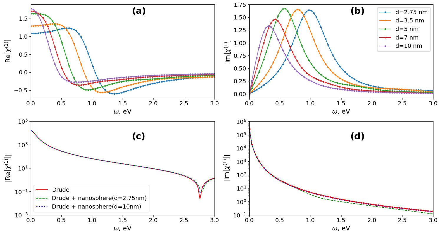
Figure 5: (a,b) Linear susceptibility due to confinement-based resonances only, in dependence on frequency for spherical nanoparticle of different diameters. (c,d) The Drude contribution as well as the full linear susceptibility (Drude + confinement) for few selected diameters.

I.6 Influence of other mechanisms

Although the approaches presented in our article is rather universal and largely material-independent, in the main paper we, to be specific, considered the parameters of gold as our basic case since gold has the most practical importance. However, gold is quite a “complicated” metal in the sense that many other mechanisms contribute to nonlinearity. Besides, in all metals, in addition to quantum-confinement (billiard-part) the Drude part of $\chi^{(1)}$ is contributing. In this section we will clarify in more detail the question how other mechanisms influence the overall nonlinear and linear response.

I.6.1 Drude part of $\chi^{(1)}$

In the Figure 2 of the main article we show the linear response without the influence of the Drude part of $\chi^{(1)}$ (the first part in the left side of Eq. (16) above, also described by Eq. (17) above). The influence of the Drude part is much larger that the confinement-based part, especially at small frequencies in MIR and THz range. In particular, Fig. 5(c,d) shows the Drude part alone and together with the quantum confinement part of the linear susceptibility for few particular diameters. One can clearly see that the Drude part absolutely dominates in the linear response at low frequencies. However, this does not mean that that the confinement-based super-resonance considered in this paper “disappears” as we take into account Drude. It can be still deconvoluted and separated from the Drude part Wyrwas et al. (2007). Besides, at it was shown in the main text, it is directly visible when considering the nonlinear optical properties such as Kerr effect.

I.6.2 Effect of interband transitions on the nonlinear response

In the main article, we considered rather simplified bandgap consisting only of one band. Whereas such approximation is very well suitable for some materials such as alkali metals, for other materials such as gold it could be claimed to be a rather bad approximation. However, at least in the particular case of gold, as soon as we consider low-frequency response, it can be shown that the nonlinearity due to interband transitions is much smaller than the one due to the billiard resonances.

In the case of gold Christensen and Seraphin (1971), there is a strong resonance in the optical response around 2.4 eV, responsible to the transitions from the 5d valence band to the 6sp conduction band, as well as a number of less pronounced resonances in the range between around 2 to 10 eV. That is, the effects of the interband transitions might be pronounced for the photon energies above 1 eV. Even at the frequency resonant with the interband transition the impact of confinement-based resonances to the rectification-like FWM processes we consider is one or two orders of magnitude larger that the effect of the interband transitions, as we will see in the next paragraphs.

Let us first consider the Kerr nonlinearity. Experimentally measured Kerr susceptibility for the photon energy around 2.3 eV, that is, close to resonance of the above mentioned transition is (for short, 100-fs-scale pulses) $\chi^{{(3)}}(\omega;\omega,\omega,-\omega)\sim 10^{-18}$ m²/V² (see for instance Boyd et al. (2014); note that in many other references long, picosecond pulses are considered, demonstrating higher nonlinearity as discussed in the subsection below). These measurements, of course, include all effects simultaneously, in particular intraband transitions and confinement-induced effects. We see that our calculations give the same order of magnitude of susceptibility for this frequency [see Fig. 3(a) of the main article] with only the confinement-based nonlinearity included. This means that the interband transitions do not dominate the intraband even at the interband resonance frequency; the impact of confinement-based resonances is of the same order of magnitude or higher.

On the other hand, as we decrease the frequency from the interband resonance towards THz range, the influence of the interband resonance quickly decreases whereas the influence of the confinement-based resonance increases [see Fig. 3(a) of the main article]. Therefore, we come to the conclusion that in the THz range the Kerr nonlinearity $\chi^{{(3)}}(\omega;\omega,\omega,-\omega)$ is indeed dominated by the confinement-based (intraband) transitions.

The same is also true for the FWM processes responsible for rectification-like effects considered in the main article: the influence of the interband transitions must be significantly smaller than of the intraband (confinement-based) ones. In order to make our estimation more quantitative at this point, we use the estimation technique described in Hache et al. (1988). We start from the Kerr process $\chi^{{(3)}}(\omega;\omega,\omega,-\omega)$ assuming it to be fully resonant to the interband transition (“worst-case scenario,” where the interband action is maximal). We consider then the processes $\chi^{{(3)}}(\delta;\omega+\delta,\omega,-2\omega)$ and $\chi^{{(3)}}(\delta;\omega,\omega,-2\omega+\delta)$. Because of the missing resonant terms in Eq. (18) (which gives a factor $\sim\omega^{2}$ in comparison to the interband resonant case) and also because of smaller population of the virtual levels (factor $\sim T^{2}_{2}$), the nonlinear susceptibility is reduced by a factor $(\omega T_{2})^{2}\sim 10^{2}$ comparing to the Kerr susceptibility at the interband resonance. Since, as it was established before, even at the interband resonance the confinement-based Kerr nonlinearity is at least of the same order of magnitude that the interband-induced Kerr nonlinearity, we therefore conclude that for the FWM processes the intraband (confinement-based) resonances are at least by the factor of 100 larger than the interband ones. Based on our calculations of the intraband nonlinearities [see Fig. 3(b) of the main article], we can estimate the interband effect to the nonlinear susceptibility for the considered FWM processes as 10^-20-10^-21 m²/V² for $\omega$ at the interband resonance (and even lower away from that resonance). This is much less than the confinement-based impact as shown in Fig. 3 of the main article.

As an alternative and fully independent method to estimate the impact of the interband transitions we introduce a gap directly into our numerical model. That is, we modify our single-band structure as the following:

$$\mathcal{E}_{nl}=\begin{cases}\mathcal{E}_{0}\alpha_{nl}^{2},&\text{if $|\alpha_{nl}|\leq\frac{2\pi}{\Lambda}$,}\\ \mathcal{E}_{0}\alpha_{nl}^{2}+E_{g},&\text{if $|\alpha_{nl}|>\frac{2\pi}{\Lambda}$,}\end{cases}$$ (21)

where $\Lambda$ is the lattice constant (for gold $\Lambda\approx 4$ Å), $E_{g}\approx 2.4$ eV. This modification mimics the bandgap which opens near the edges of the Brillouin zone. The comparison of two calculations, that is, using the single band Eq. (2) model and two band model Eq. (21), are shown in Fig. 6 for different exemplary diameters. One can see that, whereas the interband transition does provide some limited modification to the confinement-based dynamics for very small nanoparticles $d\lessapprox 3$ nm, this influence quickly decreases and becomes negligible for larger diameters.

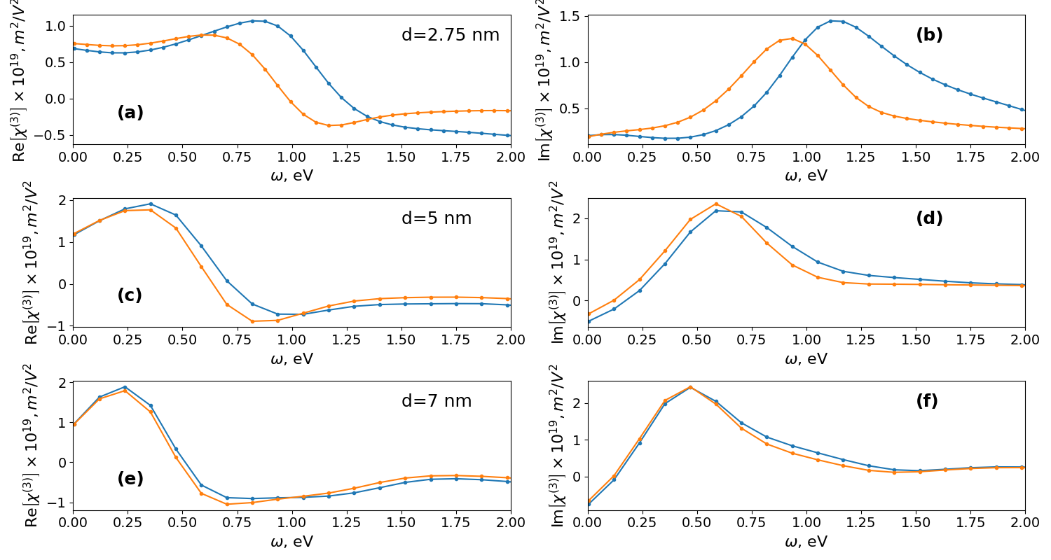
Figure 6: Real (a,c,e) and imaginary (b,d,f) part of the nonlinear susceptibility $\chi^{(3)}(\delta;\omega,\omega,-2\omega+\delta)$ for different diameters (see legend), corresponding to Fig. 3(b) of the main article, effectively taking into account (orange curves) and without taking account (blue lines) the interband transitions as introduced by Eq. (21). The latter correspond to Fig. 3(b) of the main article.

I.6.3 Thermal, hot-electron and related effects

Taking into account temperature introduces several effects, which were neglected in the main article. First of all, it leads to an additional hot-electron contribution into nonlinearly Boyd et al. (2014), which can overcome, by several orders of magnitude, the nonlinearities considered in this article up to now. The hot electron mechanism involves laser-induced intraband excitation in the conduction band, followed by the energy dissipation of the excited electrons. This process leads to a modification of Fermi-Dirac distribution which depends on the frequency and intensity of the pump, leading thereby to frequency-dependent nonlinearity Voisin et al. (2000); Besteiro et al. (2019); Hartland et al. (2017). The key role in the quick thermalization is played by the electron-electron and electron-phonon interactions.

This nonlinearity has relatively slow, sub-picosecond-scale, turn-on time Sun et al. (1994), and therefore its influence quickly decreases with decreasing of the pulse duration Boyd et al. (2014). For the pulses considered here (10-30 femtoseconds) this nonlinearity plays a negligible role. Indeed, the experimentally measured Kerr nonlinearity for gold nanospheres Boyd et al. (2014); Rotenberg et al. (2007) for the pulses of 100 fs duration corresponds, by the order of magnitude ($\sim 10^{-18}$ m²/V², see also discussion in the previous subsection) to our calculations at around the same frequency (cf. Fig. 3(a) of the main article). Since in our calculations we do not take into account the hot electron nonlinearities, we come to the conclusion that for short pulses such nonlinearities are pretty much negligible in comparison to the confinement-based resonances, or at least do not play a dominant role. This is even more true if we consider lower frequencies towards THz range, since the confinement-based nonlinearity has a resonance at low frequencies, whereas the thermal nonlinearity is not expected to demonstrate a resonant behaviour.

A part of the above-described thermalization process is the electron-electron interaction. Fast thermalization, indeed, is the primarily consequence of the electron-electron interactions Hertel et al. (1996); Hartland et al. (2017). Electron-electron interactions are trackable in the linear properties of the nanostructure (see for instance Voisin et al. (2000)), however, the corresponding modification is rather minor and even this small modification starts to be visible at the time scale of few tens of femtoseconds.

Another thermal effect is the overall non-rectangular shape of the electron distribution near the Fermi zone edge as soon as the temperature is nonzero (in our calculations in the main article we assumed zero temperature). The effect of nonzero temperature in the vicinity of Fermi-level is shown in Fig. 7 for an exemplary diameters $d=2.75$ nm and temperature $T=300$ K. It is obtained by modifying $\rho_{ll}^{(0)}$ from Eq. (19) to the Fermi-Dirac distribution for the finite temperature. One can see that this modifies only slightly the linear response. The nonlinear response is also modified quite moderately.

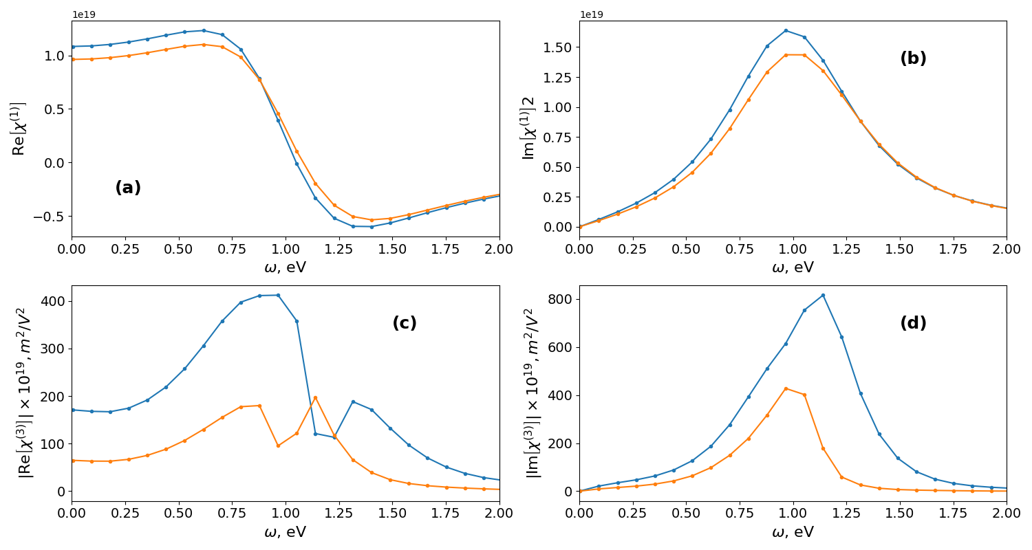
Figure 7: Real (a,c) and imaginary (b,d) part of the linear (a,b) and nonlinear (Kerr) (b,c) susceptibility for the structure $d=2.75$ assuming sharp transition at $E=\mathcal{E}_{F}$ (blue lines) and taking into account Fermi-Dirac distribution for $T=300$ K (orange lines).

I.7 Level statistics details

I.7.1 General definitions

In this section we describe different variants of the level statistics, extending the discussion related to Fig. 2 of the main article. To understand the mechanisms, governing the formation of one single super-resonance it is very constructive to consider the level statistics, varying the selection rules included into that statistics. Commonly in the quantum billiard and quantum chaos theory Stöckmann (1999) one considers the so called neighboring level statistics. That is, we consider the difference between the neighboring levels $\delta\omega_{i}=\omega_{i+1}-\omega_{i}$, where the eigenfrequencies $\omega_{i}$ are obtained by ordering of the eigenfrequencies in the increasing order, that is, we order them in such a way that $\omega_{j}\leq\omega_{i}$ for $j<i$. In the case of nanospheres the corresponding eigenvalues are $\hbar\omega_{nl}=\mathcal{E}_{nl}$, cf. Eq. (2), reaaranged accordingly. Note that $i$, $j$ here are single indices (and not multiindices as in Sec. I.4). Then, the probability $P(\omega)d\omega$ that $\delta\omega_{i}$ is located in the range between $\omega$ and $\omega+d\omega$ is calculated. The easiest way to visualize such statistics is to use the histogram technique. For nanospheres this traditional neighboring level statistics is presented in Fig. 2a of the main article (yellow bars).

The neighboring level statistics do allow to determine the universality classes of different billiards. It, however, does not take into account the properties of eigenfunctions and of the transition rules, so it seems to be of little use for the optical properties. In order to improve usability for optics, we extend the statistics to take into account all transitions, not only neighboring, and impose additional selection rules. That is, we consider the statistics of energy differences $\omega_{ij}=\omega_{i}-\omega_{j}$ for $i>j$ (assuming the ordering of $\omega_{j}$ as discussed above). In addition, when constructing the probability density $P(\omega)$ of $\omega_{ij}$ being in the interval $[\omega,\omega+d\omega]$, we take into account the “strength” of the transition by weighting $P(\omega_{ij})$ with a weight

$$w_{ij}=\Delta_{ij}|\mu_{ij}|^{2},$$ (22)

where $\mu_{ij}$ is the dipole momentum of the corresponding transition $i\to j$, and $\Delta_{ij}$ is defined as

$$\Delta_{ij}=\begin{cases}1,&\text{if $\hbar\omega_{i}\leq\mathcal{E}_{F}$ and $\hbar\omega_{j}>\mathcal{E}_{F}$}\\ 0,&\text{otherwise,}\end{cases}$$ (23)

that is, takes into account the Fermi-Dirac distribution Eq. (19) (we call it below “the Fermi sea condition”). The resulting statistics is shown in Fig. 2 (red and blue bars) and repeated for convenience as the inset in Fig. 8(a) – for the larger frequency range. We note that the traditional statistics discussed in the previous paragraph is a partial case of this more general approach; namely, we obtain the traditional neighboring level statistics assuming $w_{ij}=\delta_{i,j=i+1}$.

I.7.2 Natural shape and width of the super-resonance for nanospheres

To find out the “natural width” of the super-resonance for the case of nanostructures, we use a more more precise version of Eq. (10):

$$\alpha_{nl}=(2n+l+s_{nl})\pi/2,$$ (24)

which includes corrections $s_{nl}$ to the values of the roots. All transitions contributing to the super-resonance are characterized by the same value of $2n+l$ before and after the transition, that is, $2n^{\prime}+l^{\prime}=2n+l+1$. However, values of $n$ and $l$ can be different. Therefore the energy difference between the eigenfunctions $\left|\psi_{nl}\right\rangle$ and $\left|\psi_{n^{\prime}l^{\prime}}\right\rangle$ will be modified as follows:

$$\Delta\mathcal{E}=\frac{\pi^{2}\mathcal{E}_{0}}{4}\left[(2n^{\prime}+l^{\prime}+s_{n^{\prime}l^{\prime}})^{2}-(2n+l+s_{nl})^{2}\right]\simeq\frac{\pi^{2}\mathcal{E}_{0}}{2}(2n+l)(1+s_{n^{\prime}l^{\prime}}-s_{nl}).$$ (25)

For the typical range of $n$ and $l$ actual for our particular situation, we approximate $s_{nl}$ as being distributed in the range [-0.25,0]. For the probability distribution of the difference $s_{nl}-s_{n^{\prime}l^{\prime}}$, given by $P(s_{n^{\prime}l^{\prime}}-s_{nl})\sim\int P(s)P(s+s_{n^{\prime}l^{\prime}}-s_{nl})ds$, we obtain a triangular symmetric shape with the maximum at zero and full width of $1/2$, that is we have a constant FWHM of $1/4$ of the distribution of the difference $s_{nl}-s_{n^{\prime}l^{\prime}}$. Using Eq. (11) we obtain that this translates to the width $\approx\omega_{\mathrm{conf}}/4$ in frequency, where $\omega_{\mathrm{conf}}$ is the position of the super-resonance as defined in Eq. 1 of the main article. If we consider the dipole-momentum-weighted statistics as described below, this simplified conclusion will be modified by the fact that the dipole momentum depends on the energy level difference. Such dependence will result in sharper lower-frequency shoulder of the statistics and smoother higher-frequency shoulder. Both such shape and the width of the peak in the statistics are in a surprisingly good agreement with the findings shown in Fig. 2 of the main article (for the case of large T₂). Of course, reducing the $T_{2}$ to room-temperature values additionally increases the width of the super-resonance beyond the natural width of $\approx\omega_{\mathrm{conf}}/4$.

I.7.3 Influence of different mechanisms on the statistics

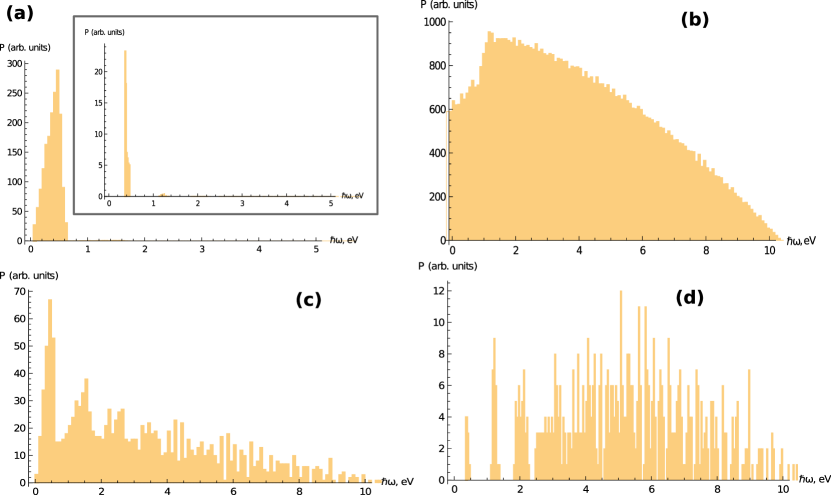
Figure 8: Different variants of level statistics. (a) $P(\omega_{ij})$ weighted as given by Eq. (22), only with $\Delta_{ij}=1$, that is not taking into account Fermi sea condition (delivering thereby the statistics for dielectrics). Inset to (a): Repetition of Fig. 1 of the main article on the larger energy scale, that is: $P(\omega_{ij})$ weighted as given by Eq. (22). (b) The same as in (a) but assuming in addition $\mu_{ji}=1$, that is, unweighted. (c) The same as in (b) but assuming $w_{ji}=0$ if $\mu_{ij}=0$ and $w_{ij}=1$ otherwise. (d) The same as in (c) but taking into account the Fermi sea restriction Eq. (23).

Varying the selection rules incorporated into the weighting Eq. (22), we can study how these rules influence the statistics. Different variants of statistics are shown in Fig. 8. In particular, in Fig. 8(a) we consider $P(\omega_{ij})$ weighted by Eq. (22) with $\Delta_{ij}=1$, that is not taking into account the Fermi sea condition – i.e. all transition, not only the transitions from the below to above the Fermi sea level, are allowed. This situation describes dielectrics rather than metals, and should be contrasted to the “metallic case”, that is, the situation where also the “Fermi sea condition” is satisfied [inset to Fig. 8(a) as well as Fig. 2a of the main article]. One can see that in the former case the resonance is much more broad and, in addition, noticeably shifted to the lower frequencies.

On the other hand, if we remove all restrictions at all, that is, consider $w_{ij}=1$ for all $i$, $j$, we will see very broad distribution over the scale of many eV Fig. 8(b). The statistics changes not too significantly if we take into account only allowed transitions (but not yet distinguishing between the strengths of the transitions, that is, assuming $w_{ji}=0$ if $\mu_{ij}=0$ and $w_{ij}=1$ otherwise, and also not taking into account the Fermi sea condition). Yet, in this case the peak, corresponding to the low-frequency super-resonance (at around 0.5 eV) does already appear [see Fig. 8(c)]. This peak becomes even sharper if we in addition take into account the Fermi sea condition as shown in Fig. 8(d). But, in addition to this low-frequency peak, in Fig. 8(d) we see also many other peaks at higher frequency. These many peaks disappear as we take into account the “strengths” of the transitions ($\mu^{2}$-weighting as given by Eq. (22)), see inset to Fig. 8(a) and Fig. 2a of the main article.

Therefore, we conclude that there is, in general, a lot of possible confinement-based transitions at low and high frequencies. The key role in the formation of a single super-resonance is played by the dipole moments, that is, by the symmetry and composition of the wavefunctions, and only to a lesser extent by the Fermi sea condition. As we take them into account, we are left with a single bunch of closely spaced resonances, which, taking into account that every of these resonances are broadband, merge into a super-resonance. Whereas the consideration here was focused on the case of nanospheres, we remark that, most probably, this particular situation is quite geometry-independent, at least for regular billiards. Indeed, in this case we expect that distantly spaced eigenfunctions have very different number of oscillations in every spatial direction, making $\mu_{ij}$ small. This, however, is not necessarily the case for the irregular, chaotic billiards which have also rather chaotic eigenfunctions. Finally, as Fig. 2(b) of the main article shows, we can tune the positions of the resonances in such a way that the resulting super-resonance is broadened.

I.8 Effective properties of nanocomposite

The effective linear properties of the nanocomposite for arbitrary frequency $\omega$ are calculated using the effective medium approach Zeng et al. (1988) using the linear properties of the host $\varepsilon_{h}(\omega)$ (in our case SiO₂), and nanostructures $\varepsilon_{\mathrm{NP}}(\omega)$ [which is given by $\varepsilon_{\mathrm{NP}}(\omega)=1+\chi^{(1)}$, where $\chi^{(1)}$ is calculated according to Eq. (16)], as:

$$\varepsilon_{\mathrm{eff}}(\omega)=\varepsilon_{h}(\omega)+fx(\omega)(\varepsilon_{\mathrm{NP}}(\omega)-\varepsilon_{h}(\omega)).$$ (26)

where $f$ is the filling factor, $x(\omega)$ is defined as

$$x(\omega)=\frac{3\varepsilon_{h}(\omega)}{\varepsilon_{\mathrm{NP}}(\omega)+2\varepsilon_{h}(\omega)}.$$ (27)

We note that at Mie resonance $|x|$ is especially large. Finally, the effective nonlinear susceptibility $\chi^{(3)}_{\mathrm{eff}}$ for every process is calculated for given linear and nonlinear properties of the nanostructures and host as follows:

$$\chi^{(3)}_{\mathrm{eff}}=f\chi^{(3)}_{\mathrm{NP}}x(\omega_{0})x_{(}\omega_{1})^{2}x(\omega_{2}),$$ (28)

where $\chi^{(3)}_{\mathrm{NP}}$ is the nonlinear susceptibility given by Eq. 5 or Eq. 6 of the main article, with $\chi^{(3)}$ in those expressions calculated using Eq. (18).

I.9 Propagation equations

Assuming slowly varying envelope approximation and neglecting nonlinear effects for the pump waves, the governing equations are:

$$\frac{\partial A_{0}}{\partial z}=-\frac{1}{2c\varepsilon_{0}}\frac{\partial P}{\partial t}=-\frac{i\delta\chi^{(3)}_{\mathrm{eff}}(\delta)}{2c}A_{1}^{2}(z)A^{*}_{2}(z)-\alpha_{0}A_{0},$$ (29)

$$\partial_{z}A_{n}=ik_{n}A_{n}-\alpha_{n}A_{n},\,n=1,2,$$ (30)

where $c$ is the speed of light in vacuum, $\varepsilon_{0}$ is vacuum permittivity, $A_{i}$, $\alpha_{i}$ $k_{i}$, $i=0,1,2$ are correspondingly the slow (complex) amplitudes, linear losses, and wavevectors for $n$th harmonic (here signal is assumed to be the “0th harmonic”), and $\chi^{(3)}_{\mathrm{eff}}(\delta)$ is the effective nonlinear susceptibility for the corresponding process. Eqs. (29)-(30) allows an analytical solution, given by:

$$A_{0}=-iAe^{-\alpha_{0}L}(e^{\kappa L}-1)/\kappa,$$ (31)

where $A=\delta\chi^{(3)}_{\mathrm{eff}}A_{1}^{2}(0)A_{2}^{*}(0)/2c$, $L$ is the propagation distance, $\kappa=i(k_{0}+2k_{1}-k_{2})-2\alpha_{1}-\alpha_{2}+\alpha_{0}$.

Assuming the pulse durations of around 30 fs, we must consider two regions for the pump where conversion works significantly differently. For the signal in the THz range ($\delta/2\pi\leq$ 30 THz), the frequencies $j\omega_{0}$ and $j\omega_{0}+\delta$ ($j=1,2$) are both located within the spectrum of the pump. The nonlinearity in this case is driven by three contribution types mentioned above, and must be considered as the following sum:

$$\chi^{(3)}_{\mathrm{NP}}(\delta)\approx\chi^{(3)}(\delta;\omega_{0},\omega_{0},-2\omega_{0}+\delta)\\ +\chi^{(3)}(\delta;\omega_{0}+\delta,\omega_{0},-2\omega_{0})+\chi^{(3)}(\delta;\omega_{0},\omega_{0}+\delta,-2\omega_{0}).$$ (32)

In contrast, for the signal in MIR range $\delta/2\pi>$ 30 THz, the components $\omega_{0}+\delta$, $2\omega_{0}+\delta$ are not within the pump spectrum anymore. In this case, in order to make the conversion efficient, we must, for instance, shift the second harmonic: $2\omega_{0}\to 2\omega_{0}+\delta$. The only effective nonlinear process in this case is

$$\chi^{(3)}_{\mathrm{NP}}(\delta)=\chi^{(3)}(\delta;\omega_{0},\omega_{0},-2\omega_{0}+\delta).$$ (33)

References

- Mie (1908) Gustav Mie, “Beiträge zur Optik trüber Medien, speziell kolloidaler Metallösungen,” Annalen der physik 330, 377–445 (1908).
- Kreibig and Vollmer (2013) Uwe Kreibig and Michael Vollmer, Optical properties of metal clusters, Vol. 25 (Springer Science & Business Media, 2013).
- Kim et al. (2010) Kwang-Hyon Kim, Anton Husakou, and Joachim Herrmann, “Linear and nonlinear optical characteristics of composites containing metal nanoparticles with different sizes and shapes,” Opt. Express 18, 7488–7496 (2010).
- Kawabata and Kubo (1966) Arisato Kawabata and Ryogo Kubo, “Electronic properties of fine metallic particles. II. Plasma resonance absorption,” J. Phys. Soc. Japan 21, 1765–1772 (1966).
- Ruppin and Yatom (1976) R. Ruppin and H. Yatom, “Size and shape effects on the broadening of the plasma resonance absorption in metals,” Phys. Status Solidi B 74, 647–654 (1976).
- Kraus and Schatz (1983) W. A. Kraus and George C. Schatz, “Plasmon resonance broadening in small metal particles,” J. Chem. Phys. 79, 6130–6139 (1983).
- Amendola et al. (2017) Vincenzo Amendola, Roberto Pilot, Marco Frasconi, Onofrio M Maragò, and Maria Antonia Iatì, “Surface plasmon resonance in gold nanoparticles: a review,” J. Phys. Condens. Matter 29, 203002 (2017).
- Scholl et al. (2012) J. Scholl, A. Koh, and J. Dionne, “Quantum plasmon resonances of individual metallic nanoparticles,” Nature 483, 421–427 (2012).
- Morton et al. (2011) Seth M Morton, Daniel W Silverstein, and Lasse Jensen, “Theoretical studies of plasmonics using electronic structure methods,” Chem. Rev. 111, 3962–3994 (2011).
- Philip et al. (2012) Reji Philip, Panit Chantharasupawong, Huifeng Qian, Rongchao Jin, and Jayan Thomas, “Evolution of nonlinear optical properties: from gold atomic clusters to plasmonic nanocrystals,” Nano Lett. 12, 4661–4667 (2012).
- Boyd et al. (2014) Robert W Boyd, Zhimin Shi, and Israel De Leon, “The third-order nonlinear optical susceptibility of gold,” Opt. Commun. 326, 74–79 (2014).
- Qian et al. (2016) Haoliang Qian, Yuzhe Xiao, and Zhaowei Liu, “Giant Kerr response of ultrathin gold films from quantum size effect,” Nat. Commun. 7, 1–6 (2016).
- Varas et al. (2016) A. Varas, P. Garcia-Gonzalez, J. Feist, F. J. G.-Vidal, and A. Rubio, “Quantum plasmonics: from jellium models to ab initio calculations,” Nanophotonics 5, 409–426 (2016).
- Zhou et al. (2021) Meng Zhou, Xiangsha Du, He Wang, and Rongchao Jin, “The critical number of gold atoms for a metallic state nanocluster: Resolving a decades-long question,” ACS nano 15, 13980–13992 (2021).
- Wood and Ashcroft (1982) D. M. Wood and N. W. Ashcroft, “Quantum size effects in the optical properties of small metallic particles,” Phys. Rev. B 25, 6255–6274 (1982).
- Hache et al. (1986) F. Hache, D. Ricard, and Ch. Flytzanis, “Optical nonlinearities of small metal particles: surface-mediated resonance and quantum size effects,” JOSA B 3, 1647–1655 (1986).
- Sato et al. (2015) Rodrigo Sato, Masato Ohnuma, Keiji Oyoshi, and Yoshihiko Takeda, “Spectral investigation of nonlinear local field effects in Ag nanoparticles,” J. Appl. Phys. 117, 113101 (2015).
- Genzel et al. (1975) L. Genzel, T. P. Martin, and U. Kreibig, “Dielectric function and plasma resonances of small metal particles,” Zeitschrift für Physik B Condensed Matter 21, 339–346 (1975).
- Brack (1993) Matthias Brack, “The physics of simple metal clusters: self-consistent jellium model and semiclassical approaches,” Rev. Mod. Phys. 65, 677–732 (1993).
- Ginzburg et al. (2014) Pavel Ginzburg, Alexey V Krasavin, Gregory A Wurtz, and Anatoly V Zayats, “Nonperturbative hydrodynamic model for multiple harmonics generation in metallic nanostructures,” ACS Photonics 2, 8–13 (2014).
- Hurst et al. (2014) Jérôme Hurst, Fernando Haas, Giovanni Manfredi, and Paul-Antoine Hervieux, “High-harmonic generation by nonlinear resonant excitation of surface plasmon modes in metallic nanoparticles,” Phys. Rev. B 89, 161111 (2014).
- Takeuchi and Yabana (2022) Takashi Takeuchi and Kazuhiro Yabana, “Electron spill-out effect on third-order optical nonlinearity of metallic nanostructure,” Phys. Rev. A 106, 063517 (2022).
- Zhang et al. (2017) Xu Zhang, Hongping Xiang, Mingliang Zhang, and Gang Lu, “Plasmonic resonances of nanoparticles from large-scale quantum mechanical simulations,” International Journal of Modern Physics B 31, 1740003 (2017).
- Barbry et al. (2015) M. Barbry, P. Koval, F Marchesin, R. Esteban, A. G. Borisov, J. Aizpurua, and D Sanchez-Portal, “Atomistic near-field nanoplasmonics: Reaching atomic-scale resolution in nanooptics,” Nano Lett. 15, 3410–3419 (2015).
- Rossi et al. (2017) T. P. Rossi, M Kuisma, M. J. Puska, Nieminen R. M., and P. Erhart, “Kohn–sham decomposition in real-time time-dependent density-functional theory: An efficient tool for analyzing plasmonic excitation,” J. Chem. Theory Comput. 13, 4779–4790 (2017).
- Day et al. (2010) Paul N Day, Kiet A Nguyen, and Ruth Pachter, “Calculation of one-and two-photon absorption spectra of thiolated gold nanoclusters using time-dependent density functional theory,” J. Chem. Theor. Comput. 6, 2809–2821 (2010).
- Day et al. (2016) Paul N Day, Ruth Pachter, Kiet A Nguyen, and Terry P Bigioni, “Linear and nonlinear optical response in silver nanoclusters: insight from a computational investigation,” J. Phys. Chem. A 120, 507–518 (2016).
- Zhou et al. (2016) Meng Zhou, Chenjie Zeng, Yuxiang Chen, Shuo Zhao, Matthew Y Sfeir, Manzhou Zhu, and Rongchao Jin, “Evolution from the plasmon to exciton state in ligand-protected atomically precise gold nanoparticles,” Nat. Commun. 7, 1–7 (2016).
- Townsend and Bryant (2012) E. Townsend and G. W. Bryant, “Plasmonic properties of metallic nanoparticles: The effects of size quantization,” Nano Lett. 12, 429–434 (2012).
- Barcaro et al. (2006) Giovanni Barcaro, Alessandro Fortunelli, Giulia Rossi, Florin Nita, and Riccardo Ferrando, “Electronic and structural shell closure in AgCu and AuCu nanoclusters,” J. Phys. Chem. B 110, 23197–23203 (2006).
- Kwak et al. (2017) Kyuju Kwak, Viraj Dhanushka Thanthirige, Kyunglim Pyo, Dongil Lee, and Guda Ramakrishna, “Energy gap law for exciton dynamics in gold cluster molecules,” J. Phys. Chem. Lett. 8, 4898–4905 (2017).
- Zhou et al. (2019) Meng Zhou, Tatsuya Higaki, Yingwei Li, Chenjie Zeng, Qi Li, Matthew Y. Sfeir, and Rongchao Jin, “Three-stage evolution from nonscalable to scalable optical properties of thiolate-protected gold nanoclusters,” J. Am. Chem. Soc. 141, 19754–19764 (2019).
- Oates and Mücklich (2005) T. W. H. Oates and A. Mücklich, “Evolution of plasmon resonances during plasma deposition of silver nanoparticles,” Nanotechnology 16, 2606 (2005).
- Wyrwas et al. (2007) R. B. Wyrwas, M. M. Alvarez, J. T. Khoury, R. C. Price, T. G. Schaaff, and R. L. Whetten, “The colours of nanometric gold,” Eur. Phys. J. D 43, 91–95 (2007).
- He and Zeng (2010) Yi He and Taofang Zeng, “First-principles study and model of dielectric functions of silver nanoparticles,” J. Phys. Chem. C 114, 18023–18030 (2010).
- Stöckmann (1999) Hans-Jürgen Stöckmann, Quantum Chaos: An Introduction (Cambridge University Press, New York, USA, 1999).
- Simons and Altshuler (1993) B. D. Simons and B. L. Altshuler, “Universalities in the spectra of disordered and chaotic systems,” Phys. Rev. B 48, 5422–5438 (1993).
- Ravnik et al. (2021) Jan Ravnik, Yevhenii Vaskivskyi, Jaka Vodeb, Polona Aupič, Igor Vaskivskyi, Denis Golež, Yaroslav Gerasimenko, Viktor Kabanov, and Dragan Mihailovic, “Quantum billiards with correlated electrons confined in triangular transition metal dichalcogenide monolayer nanostructures,” Nat. Commun. 12, 1–8 (2021).
- Nakamura and Thomas (1988) K. Nakamura and H. Thomas, “Quantum billiard in a magnetic field: Chaos and diamagnetism,” Phys. Rev. Lett. 61, 247–250 (1988).
- Jalabert et al. (1990) Rodolfo A. Jalabert, Harold U. Baranger, and A. Douglas Stone, “Conductance fluctuations in the ballistic regime: A probe of quantum chaos?” Phys. Rev. Lett. 65, 2442–2445 (1990).
- Akis et al. (1997) R. Akis, D. K. Ferry, and J. P. Bird, “Wave function scarring effects in open stadium shaped quantum dots,” Phys. Rev. Lett. 79, 123–126 (1997).
- Zozoulenko and Berggren (1997) I. V. Zozoulenko and K.-F. Berggren, “Quantum scattering, resonant states, and conductance fluctuations in an open square electron billiard,” Phys. Rev. B 56, 6931–6941 (1997).
- Burke et al. (2010) A. M. Burke, R. Akis, T. E. Day, Gil Speyer, D. K. Ferry, and B. R. Bennett, “Periodic scarred states in open quantum dots as evidence of quantum darwinism,” Phys. Rev. Lett. 104, 176801 (2010).
- Ponomarenko et al. (2008) L. A. Ponomarenko, F. Schedin, M. I. Katsnelson, R. Yang, E. W. Hill, K. S. Novoselov, and A. K. Geim, “Chaotic Dirac Billiard in Graphene Quantum Dots,” Science 320, 356–358 (2008).
- Kuchařík et al. (2019) Jiří Kuchařík, Hynek Němec, and Tomáš Ostatnickỳ, “Terahertz conductivity and coupling between geometrical and plasmonic resonances in nanostructures,” Phys. Rev. B 99, 035407 (2019).
- Boyd and Prato (2008) R.W. Boyd and D. Prato, Nonlinear Optics (Elsevier Science, 2008).
- Kabanov and Alexandrov (2008) V. V. Kabanov and A. S. Alexandrov, “Electron relaxation in metals: Theory and exact analytical solutions,” Phys. Rev. B 78, 174514 (2008).
- Kuchařík and Němec (2021) Jiří Kuchařík and Hynek Němec, “Strong confinement-induced nonlinear terahertz response in semiconductor nanostructures revealed by monte carlo calculations,” Phys. Rev. B 103, 205426 (2021).
- Zeng et al. (1988) X. C. Zeng, D. J. Bergman, P. M. Hui, and D. Stroud, “Effective-medium theory for weakly nonlinear composites,” Phys. Rev. B 38, 10970 (1988).
- Palik (1998) Edward D Palik, Handbook of optical constants of solids, Vol. 3 (Academic press, 1998).
- Poole et al. (2013) Patrick Poole, Simeon Trendafilov, Gennady Shvets, Douglas Smith, and Enam Chowdhury, “Femtosecond laser damage threshold of pulse compression gratings for petawatt scale laser systems,” Optics express 21, 26341–26351 (2013).
- Chimier et al. (2011) B. Chimier, O. Utéza, N. Sanner, M. Sentis, T. Itina, P. Lassonde, F. Légaré, F. Vidal, and J. C. Kieffer, “Damage and ablation thresholds of fused-silica in femtosecond regime,” Phys. Rev. B 84, 094104 (2011).
- Luo et al. (2014) Liang Luo, Ioannis Chatzakis, Jigang Wang, Fabian BP Niesler, Martin Wegener, Thomas Koschny, and Costas M Soukoulis, “Broadband terahertz generation from metamaterials,” Nat. Commun. 5, 3055 (2014).
- Keren-Zur et al. (2019) Shay Keren-Zur, Mai Tal, Sharly Fleischer, Daniel M Mittleman, and Tal Ellenbogen, “Generation of spatiotemporally tailored terahertz wavepackets by nonlinear metasurfaces,” Nat. Commun. 10, 1778 (2019).
- Samizadeh Nikoo and Matioli (2023) Mohammad Samizadeh Nikoo and Elison Matioli, “Electronic metadevices for terahertz applications,” Nature 614, 451–455 (2023).
- Okamoto (2021) Katsunari Okamoto, Fundamentals of optical waveguides (Elsevier, 2021).
- Kitamura (2015) Hikaru Kitamura, “Derivation of the drude conductivity from quantum kinetic equations,” Eur. J. Phys. 36, 065010 (2015).
- Sönnichsen (2001) Carsten Sönnichsen, Plasmons in metal nanostructures, Ph.D. thesis, lmu (2001).
- Christensen and Seraphin (1971) N. Egede Christensen and B. O. Seraphin, “Relativistic band calculation and the optical properties of gold,” Phys. Rev. B 4, 3321–3344 (1971).
- Hache et al. (1988) F. Hache, D Ricard, Ch Flytzanis, and U Kreibig, “The optical Kerr effect in small metal particles and metal colloids: the case of gold,” Appl. Phys. A 47, 347–357 (1988).
- Voisin et al. (2000) C. Voisin, D. Christofilos, N. Del Fatti, F. Vallée, B. Prével, E. Cottancin, J. Lermé, M. Pellarin, and M. Broyer, “Size-dependent electron-electron interactions in metal nanoparticles,” Phys. Rev. Lett. 85, 2200–2203 (2000).
- Besteiro et al. (2019) Lucas V Besteiro, Peng Yu, Zhiming Wang, Alexander W Holleitner, Gregory V Hartland, Gary P Wiederrecht, and Alexander O Govorov, “The fast and the furious: Ultrafast hot electrons in plasmonic metastructures. size and structure matter,” Nano Today 27, 120–145 (2019).
- Hartland et al. (2017) Gregory V Hartland, Lucas V Besteiro, Paul Johns, and Alexander O Govorov, “What’s so hot about electrons in metal nanoparticles?” ACS Energy Lett. 2, 1641–1653 (2017).
- Sun et al. (1994) C.-K. Sun, F. Vallée, L. H. Acioli, E. P. Ippen, and J. G. Fujimoto, “Femtosecond-tunable measurement of electron thermalization in gold,” Phys. Rev. B 50, 15337 (1994).
- Rotenberg et al. (2007) Nir Rotenberg, A. D. Bristow, Markus Pfeiffer, Markus Betz, and H. M. van Driel, “Nonlinear absorption in au films: Role of thermal effects,” Phys. Rev. B 75, 155426 (2007).
- Hertel et al. (1996) T. Hertel, E. Knoesel, M. Wolf, and G. Ertl, “Ultrafast electron dynamics at Cu(111): Response of an electron gas to optical excitation,” Phys. Rev. Lett. 76, 535–538 (1996).