Pseudogap phase and fractionalization: Predictions for Josephson junction setup

Abstract

The pseudogap regime of the underdoped cuprates arguably remains one of the most enigmatic phenomena of correlated quantum matter. Recent theoretical ideas suggest that a pair density wave (PDW) or a “fractionalized PDW” could be a key ingredient for the understanding of the pseudogap physics. These ideas are to be contrasted to the scenario where charge density wave order and superconductivity coexist at low temperatures. In this paper, we present a few tests to compare the two scenarios in a Josephson junction setup. For a PDW scenario, we observe a beat-like structure of AC Josephson current. The additional frequencies for the AC Josephson current appear at the half-odd integer multiple of the standard Josephson frequency. We can extract the modulation wavevector of the PDW state by studying the average Josephson current. Furthermore, the usual sharp Shapiro steps break down. In contrast, these signatures are absent for the simple coexistence of orders. Any detection of such signatures in a similar experimental setup will strongly support the PDW scenario for the pseudogap phase.

I Introduction

One of the most unusual features of the cuprates is the proliferation of quasi-degenerate orders in the underdoped regime near the mysterious pseudogap (PG) phase Alloul et al. (1989, 1991); Warren et al. (1989). These include experimentally established orders, like superconductivity (SC), charge density wave (CDW), and antiferromagnetism. Additionally, it may also harbor putative “hidden” orders like the pair density wave (PDW) state, for which experimental evidence is still lacking. Conceptually, it is natural to advocate that a very unusual interplay of states is responsible for the formation of the PG Loret et al. (2019). Many routes are proposed to drive forward this set of ideas.

Firstly there are the proposals of a vestigial order Fernandes et al. (2019); Fradkin et al. (2015); Sachdev and La Placa (2013); Allais et al. (2014a, b); Chien et al. (2009). In this framework, the system forms all the potentially degenerate orders. These orders compete within a standard Ginzburg-Landau description, resulting in some precursor order that can account for the development of the pseudogap state. For example, in this scenario, the competition between the SC and CDW state can lead to a precursor state formed by a long-ranged PDW order Du et al. (2020); Shi et al. (2020); Lozano et al. (2021).

A more unconventional proposal affirms that such appearance of quasi-degenerate states can lead to an emergent symmetry Scheurer et al. (2018); Sachdev et al. (2019); Nussinov and Zaanen (2002); Zaanen and Nussinov (2003); Lee et al. (1998); Dai et al. (2018); Wang et al. (2015). Concretely, considering only the SC and CDW orders for simplicity, the corresponding emergent symmetry is the SU(2) group, rotating between the two states. However, this emergent symmetry is fragile and it is easily destroyed by a slight tuning of appropriate parameters. Nevertheless, the idea of an emergent symmetry is the first illustration of the presence of some entangled states, in this particular case the SC and CDW states, which is undoubtedly present in the cuprates. Indeed some proposals have suggested that around optimal doping, the cuprate superconductors form a maximally entangled state which is associated with a strong coupling fixed point that can be accessed within the holographic framework Hartnoll et al. (2018).

Somewhere in-between the ideas of an ultimately entangled fixed point and a vestigial order remains yet another proposal Chakraborty et al. (2019); Grandadam et al. (2020a); Pépin et al. (2020); Grandadam et al. (2020b). In this approach, at $T^{*}$ the system is ripe to form all possible particle-particle (PP) and particle-hole pairs that symmetry allows. This includes PP pairs with zero and finite momentum, particle-hole (PH) pairs with finite momentum, some of which are magnetically inert and others active. Some preformed pairs become unstable and fractionalize into more robust pairs at lower temperatures. A gauge field emerges, and the corresponding constraint generated by the fluctuations leads to the opening of a gap and, thus, to the pseudogap phase itself. The rest of the introduction highlights the critical differences between fractionalized PDW and coexisting order scenarios.

I.1 Theoretical concepts for “fractionalized” PDW and coexisting orders

We focus on the idea of a PDW preformed pair, fractionalizing into a CDW and SC pairs. The choice has the advantage of simplicity since these two orders are ubiquitously observed Hamidian et al. (2016); Hoffman et al. (2002); Wise et al. (2008); Wen et al. (2019); Wu et al. (2015); Lin et al. (2020) inside the PG region. The CDW pair is given by ${\hat{\chi}_{ij}=g_{\chi}\hat{d}_{ij}\sum_{\sigma}c_{\mathbf{i},\sigma}^{\dagger}c_{j,\sigma}}e^{i\mathbf{Q}_{0}.(\mathbf{r_{i}}+\mathbf{r_{j}})/2}$ where $i,j$ are the nearest neighbor bonds with $\mathbf{Q}_{0}$ being the modulation wave vector, and $g_{\chi}$ the interaction responsible for forming CDW pairs. $\hat{d}_{ij}$ is the form factor with a d-wave symmetry. Similarly, the SC pairs is defined as ${\hat{\Delta}_{ij}=g_{\Delta}\hat{d}_{ij}\sum_{\sigma}\sigma c_{i,\sigma}c_{j,-\sigma}}$, where $c^{\dagger}$ ($c$) are the standard creation (annihilation) operators for electrons and $g_{\Delta}$ is the interaction forming the Cooper pairs. The origin of such unstable boson at high temperature most certainly comes from the strong coupling regime of the electrons Baskaran and Anderson (1988); Lee and Nagaosa (1992); Yang et al. (2009) but this is not the main focus of the paper. The PDW is defined as $\hat{\Delta}_{{\rm PDW}}=g_{{\rm PDW}}c_{i\downarrow}c_{i\uparrow}e^{i\mathbf{Q}_{0}.(\mathbf{r_{i}}+\mathbf{r_{j}})/2}$. It turns out that it can be written as a combination of elementary operators, i.e., $\hat{\Delta}_{{\rm PDW}}^{*}=\frac{g_{{\rm PDW}}}{2g_{\Delta}g_{\chi}}\left[\hat{\Delta}_{ij},\hat{\chi}_{ij}^{*}\right]$ and $\hat{\Delta}_{{\rm PDW}}=\frac{g_{{\rm PDW}}}{2g_{\Delta}g_{\chi}}\left[\hat{\chi}_{ij},\hat{\Delta}_{ij}^{*}\right]$ where $\left[a,b\right]$ stands for the commutator of the operators a and b.

The key idea leading to the fractionalization of the PDW is that at the PG temperature $T^{*}$ a gauge field (or, equivalently, a local phase) emerges

$$\hat{\Delta}_{ij} \rightarrow\hat{\Delta}_{r}e^{i\theta_{ij}},$$

$$\hat{\chi}_{ij} \rightarrow\hat{\chi}_{r}e^{i\theta_{ij}},$$ (1)

and $\hat{\Delta}_{{\rm PDW}}$ and $\hat{\Delta}_{{\rm PDW}}^{*}$ remain invariant under these transformations. Fluctuations of the gauge field in an effective field theory generates a constraint (note that the $\Delta$ and $\chi$ have the dimension of energy)

$$\left|\Delta_{r}\right|^{2}+\left|\chi_{r}\right|^{2} =\left(E^{*}\right)^{2},$$ (2)

where $E^{*}$ is an energy scale typical of the PG, which is constant in temperature, and with respect to spatial variations, but doping dependent. Note that $\Delta_{r}$ ($\chi_{r}$) are the local expectation value of the $\hat{\Delta}$ ($\hat{\chi}$) at position $r$. When the coupling to the conduction electrons is considered, the constraint of Eq.(2) opens a gap, primarily in the anti-nodal (AN) region of the Fermi surface, leading to the presence of Fermi arcs in the nodal region Chakraborty et al. (2019); Grandadam et al. (2020a); Pépin et al. (2020); Grandadam et al. (2020b). In the temperature regime, $T^{*}>T>T_{co}$, the spatial expectation values of $\langle\Delta_{r}\rangle=0$ and $\langle\chi_{r}\rangle=0$ as well as the relative phase remains fluctuating.

The typical effective field theory describing the $\hat{\Delta}_{{\rm PDW}}$- mode, has the form of a quantum rotor model Chakraborty et al. (2019)

$$S =\frac{1}{2}\int d^{2}x\sum_{a,b=1}^{2}\left|\omega_{ab}\right|^{2},$$

with $$\omega_{ab}=z_{a}\partial_{\mu}z_{b}-z_{b}\partial_{\mu}z_{a},$$ (3)

with $z_{1}=\Delta/E^{*}$, $z_{2}=\chi/E^{*}$, $z_{1}^{*}=\Delta^{*}/E^{*}$, $z_{2}^{*}=\chi^{*}/E^{*}$. Note that $E^{*}$ is a real quantity associated with the PG energy scale. The gauge fluctuations within the transformation $z_{a}\rightarrow z_{a}e^{i\theta}$, ($z_{a}^{*}\rightarrow z_{a}^{*}e^{-i\theta}$) are naturally described by the constraint $\sum_{a}\left|z_{a}\right|^{2}=C$, (where $C$ is a constant), equivalent to Eq.(2). The model Eq.(3) is formally equivalent to the $\mbox{CP}^{1}$ model

$$S= \int d^{2}x\left|D_{\mu}\psi\right|^{2},$$ (4)

with $$D_{\mu}=\partial_{\mu}-i\alpha_{\mu},$$

and $$\alpha_{\mu}=\frac{1}{2}\sum_{a}z_{a}^{*}\partial_{\mu}z_{a}-z_{a}\partial_{\mu}z_{a}^{*},$$

with $\psi=\left(z_{1},z_{2}\right)^{T}$ Perelomov (1981). The model in Eq.(4) is, in turn, almost the same as a non-linear $\sigma$-model, but with an additional gauge field $\alpha$ taking care of the intrinsic U(1) gauge symmetry.

By contrast in the model of coexisting phases the action takes the form of a standard $\varphi^{4}$-field theory

$$S =\frac{1}{2}\int d^{2}x\sum_{a=1}^{2}\left(\left|\partial_{\mu}z_{a}\right|^{2}+\mu_{a}\left|z_{a}\right|^{2}\right)$$

$$+\sum_{a,b=1}^{2}g_{ab}\left|z_{a}\right|^{2}\left|z_{b}\right|^{2}.$$ (5)

In Eq.(5) the two modes are in coexistence and interact with each other, but there is no form of chirality and no emerging gauge field as in Eq. (3).

I.2 Difference between fractionalized PDW and coexistence

We focus on the underdoped cuprate superconductors within the two scenarios mentioned above for the PG Alloul et al. (1989, 1991); Warren et al. (1989). However, note that the reality is undoubtedly much more complicated than that due to the proximity to the Mott transition. Nevertheless, here, we restrict ourselves to discuss these two sets of ideas and this simplifies the following analysis enormously.

In the coexistence scenario, a precursor of the SC or the CDW orders forms at $T^{*}$. Most of the theories Fradkin et al. (2015); Agterberg et al. (2020) that have been advanced so far consider the PDW as a precursor state at $T^{*}$. Variational calculations on the $tJ$-model show that the ground state energy of the PDW state is slightly higher than the ground state energy associated with the uniform superconductivity regime Corboz et al. (2014); Choubey et al. (2017). Thus, the uniform PDW state is very difficult to stabilize at low temperatures. Some studies Agterberg et al. (2020) suggest that a locally fluctuating PDW state is responsible for opening up a pseudogap in the anti-nodal regions without ever being the true ground state. At a lower temperature $T_{co}$, two-dimensional charge modulations do form Doiron-Leyraud et al. (2007); Blanco-Canosa et al. (2013); Sebastian et al. (2012); Chang et al. (2016); Wu et al. (2011) but they have a short ranged nature. A genuine three-dimensional charge order only forms under an applied magnetic field Gerber et al. (2015); Chang et al. (2016); Machida et al. (2016). However, at zero fields, the phase of the CDW is fluctuating rapidly in space and this produces a very inhomogeneous density-wave pattern, such as, $\chi\cos\left(\mathbf{Q}_{0}\cdot\mathbf{r}+\phi_{r}\right)$ with $\phi_{r}$ strongly varying from site to site Torchinsky et al. (2013); Nie et al. (2014, 2015); Banerjee et al. (2018); Campi et al. (2015). The SC order forms at $T_{c}$, leading to the freezing of the SC phase $\Delta\exp\left(i\theta_{EM}\right)$, due to the usual Meissner effect.The phase gradient gets minimally coupled to the external EM vector potential through a term $n_{s}\left(\partial_{\mu}\theta_{EM}-2e\mathbf{A}\right)^{2}$ (where $n_{s}$ is the superfluid density). Then through a gauge transformation, the vector potential becomes massive, and the SC phase $\theta_{EM}$ gets uniform through the sample. However, in the coexistence scenario, even below $T_{c}$ the CDW order has no mechanism to have a uniform phase and should suffer phase fluctuatuations from site to site. Hence, for the simple coexistence scenario, the entanglement of the PP and PH pairs is expected to be vanishingly small.

In contrast, in the fractionalization scenario Chakraborty et al. (2019); Grandadam et al. (2020a); Pépin et al. (2020); Grandadam et al. (2020b), the PDW order fails to form at $T^{*}$. However, a gauge field (or local phase) emerges, leading to the constraint of Eq. (2). The difference between the two scenarios sets in below $T_{c}$, where the two orders coexist. We have now two orders which are related by an emergent gauge field (or, equivalently, by a local phase $\theta$) : $\chi\exp\left(i\theta\right)$ and $\Delta\exp\left(i\left(\theta+\theta_{EM}\right)\right)$. The local phase $\theta$ is minimally coupled to a neutral vector potential through the term $n_{\chi}\left(\partial_{\mu}\theta-e^{*}\mathbf{a}\right)^{2}$ (where $n_{\chi}$ is the CDW density and $e^{*}$ is the fictitious charge). On the other hand, the SC part has a term $n_{s}\left(\partial_{\mu}\theta+\partial_{\mu}\theta_{EM}-e^{*}\mathbf{a}-2e\mathbf{A}\right)^{2}$. When both orders coexist below $T_{c}$ both vector potentials $\mathbf{a}$ and $\mathbf{a}+\mathbf{A}$ become massive and are expelled from the sample; in other words, both phases $\theta$ and $\theta_{EM}$ become uniform, and insensitive to impurities Chakraborty et al. (2019). Effectively the CDW becomes active to the external EM field and behaves as a PDW. In the fractionalization scenario, a strong entanglement thus exists between the PP and PH pairs. Recently a study reported Edkins et al. (2019) an intriguing observation of an uniform CDW phase inside vortices, and this can be explained by the fractionalized PDW scenario Chakraborty et al. (2019). In this study, we consider another consequence of a fractionalized PDW: namely, its effects on the current in a Josephson junction setup.

II Model and Method

We propose the experimental setup pictured in Fig. (1). A Josephson junction (JJ) is considered, with underdoped cuprates compounds in two terminals A and B separated by an insulating material. Below $T^{*}$, the terminals in A and B access the PG regime and we expect these terminals to display both SC and CDW orders at low temperatures. The JJ is oriented such that the modulation wave vector is parallel to the junction. Moreover, in the present situation, an electric field $\mathbf{E}$ is applied in the same direction as CDW wavevector $\mathbf{Q}_{0}$.

Figure 1: Josephson junction setup when the applied electric field is parallel to the charge density wave modulation wavevector $\mathbf{Q}_{0}$. The different possible hoppings between the pairs are presented schematically. $\kappa$ denotes a PP-pair hopping from terminal A to B, and vice versa. $\kappa^{\prime}$ represents the same for the hopping of PH-pairs across the junction. The inter-junction conversion of PP-pair to a PH-pair is denoted by $t_{1}$ and the same within the junction by $t_{0}$.

We consider the following wavefunctions for the A and B subsystems

$$\ket{\psi_{A}} =\sqrt{n_{A}}e^{i\theta_{A}}+\sqrt{n_{A}^{\prime}}e^{i\theta_{A}^{\prime}},$$

$$\ket{\psi_{B}} =\sqrt{n_{B}}e^{i\theta_{B}}+\sqrt{n_{B}^{\prime}}e^{i\theta_{B}^{\prime}},$$ (6)

where $\left(n_{A,B},\theta_{A,B}\right)$ are the superfluid density and phases of SC states on terminals A and B respectively, and $\left(n_{A,B}^{\prime},\theta_{A,B}^{\prime}\right)$ are the corresponding CDW density and phases. At a steady state, we take $\theta_{A}^{\prime}=\mathbf{Q}_{0}\cdot\mathbf{r}$ and $\theta_{B}^{\prime}=\mathbf{Q}_{0}\cdot\left(\mathbf{r}+\mathbf{\delta}\right)$. The most generic set of Schrödinger’s equations Barone and Paterno (1982); Grüner (1988) that can be written with these two orders, with $\overline{\psi}=\left(\begin{array}[]{cccc}\sqrt{n_{A}}e^{i\theta_{A}},&\sqrt{n_{B}}e^{i\theta_{B}},&\sqrt{n_{A}^{\prime}}e^{i\theta_{A}^{\prime}},&\sqrt{n_{B}^{\prime}}e^{i\theta_{B}^{\prime}}\end{array}\right)$

$$i\hbar\frac{\partial}{\partial t}\psi =\left(\begin{array}[]{cccc}\mu_{\Delta}&\kappa&t_{0}&t_{1}\\ \kappa&-\mu_{\Delta}&t_{1}&t_{0}\\ t_{0}&t_{1}&V_{A}&\kappa^{\prime}\\ t_{1}&t_{0}&\kappa^{\prime}&V_{B}\end{array}\right)\psi,$$ (11)

where $\kappa$ and $\kappa^{\prime}$ are the hopping integrals for particle-particle (PP) and particle-hole (PH) pairs across the junctions. The parameter $\mu_{\Delta}=eU$, where $U$ is the electrical potential applied to the PP pairs. In terms of the applied electric field $\mathbf{E}$, this becomes $\mu_{\Delta}=-e\mathbf{E}r_{A,B}$, where $r_{A,B}$ is the distance with respect to the center. However, in this study, $\mu_{\Delta}$ is assumed to be a constant as in the standard JJ setup Barone and Paterno (1982). The parameter $t_{1}$ represents the tunneling between the PP pairs in the junction A (resp. B) to the modulated PH pairs in junction B (resp. A), whereas $t_{0}$ is the same type of tunneling within a junction. The electric field acts on the CDW sector Lee and Rice (1979) as $V_{A,B}=eE\bar{\rho}\theta_{A,B}^{\prime}$, where $\bar{\rho}=n^{\prime}/Q_{0}$ is an effective CDW density divided by the ordering wave vector $\mathbf{Q}_{0}$. We have assumed that the superfluid density and the CDW densities are constant throughout the JJ. Although this is not necessary; such assumption simplifies the following analysis enormously. Equations (11) can be decoupled into (for details see Appendix (A))

$$\frac{\partial\bar{n}}{\partial t}=\frac{4}{\hbar} \left[-\kappa n\sin{\theta}+\sqrt{nn^{\prime}}\cos{\frac{\phi}{2}}\right.$$

$$\left.\times\left(t_{0}\sin{\frac{\theta^{\prime}-\theta}{2}}-t_{1}\sin{\frac{\theta^{\prime}+\theta}{2}}\right)\right],$$ (12)

$$\frac{\partial\theta}{\partial t}=\frac{2}{\hbar} \left[\mu_{\Delta}+\sqrt{\frac{n^{\prime}}{n}}\sin{\frac{\phi}{2}}\right.$$

$$\left.\times\left(t_{0}\sin{\frac{\theta^{\prime}-\theta}{2}}-t_{1}\sin{\frac{\theta+\theta^{\prime}}{2}}\right)\right],$$ (13)

$$\frac{\partial\bar{n}^{\prime}}{\partial t}=\frac{4}{\hbar} \left[-\kappa^{\prime}n^{\prime}\sin{\theta^{\prime}}+\sqrt{nn^{\prime}}\cos{\frac{\phi}{2}}\right.$$

$$\left.\times\left(t_{0}\sin{\frac{\theta-\theta^{\prime}}{2}}-t_{1}\sin{\frac{\theta^{\prime}+\theta}{2}}\right)\right],$$ (14)

$$\frac{\partial\theta^{\prime}}{\partial t}=\frac{1}{\hbar} \left[(V_{A}-V_{B})-2\sqrt{\frac{n^{\prime}}{n}}\sin{\frac{\phi}{2}}\right.$$

$$\left.\times\left(t_{0}\sin{\frac{\theta-\theta^{\prime}}{2}}-t_{1}\sin{\frac{\theta^{\prime}+\theta}{2}}\right)\right],$$ (15)

$$\frac{\partial\phi}{\partial t}= -\frac{1}{\hbar}\left[(V_{A}+V_{B})+2\kappa\cos{\theta}+2\kappa^{\prime}\cos{\theta^{\prime}}\right.$$

$$\left.-\frac{2\delta n}{\sqrt{nn^{\prime}}}\left(t_{0}\cos{\frac{\theta-\theta^{\prime}}{2}}+t_{1}\cos{\frac{\theta+\theta^{\prime}}{2}}\right)\right],$$ (16)

with $\theta=\theta_{B}-\theta_{A}$, $\theta^{\prime}=\theta_{B}^{\prime}-\theta_{A}^{\prime}$ ,$\phi=\theta_{B}^{\prime}+\theta_{A}^{\prime}-\theta_{A}-\theta_{B}$, $\bar{n}=n_{B}-n_{A}$, $\bar{n}^{\prime}=n_{A}^{\prime}-n_{B}^{\prime}$, $\delta n=n^{\prime}-n$. Furthermore, we assumed that the density of PP-pairs and PH-pairs in both the terminal are similar, i.e. $n\simeq n_{A}\simeq n_{B}$, $n^{\prime}\simeq n_{A}^{\prime}\simeq n_{B}^{\prime}$. The variation of $\phi$ can be simplified further in the limit where $n\simeq n^{\prime}$, $\delta n\ll n$. In this limit, the Eq. (16) simplifies to,

$$\frac{\partial\phi}{\partial t}\approx -\frac{1}{\hbar}\left[(V_{A}+V_{B})+2\kappa\cos{\theta}+2\kappa^{\prime}\cos{\theta^{\prime}}\right].$$ (17)

Next we elucidate on the other parameters. The difference of the electric field on the CDW sector can be simplified to ${V_{A}-V_{B}=-(eEn^{\prime}/Q_{0})\theta^{\prime}\equiv-r_{0}\theta^{\prime}}$, where we have introduced a new parameter $r_{0}=eEn^{\prime}/Q_{0}$. Similarly, the average potential acting on the CDW sector due to the applied electric field can be treated as constant, i.e. $V_{A}+V_{B}=\eta$.

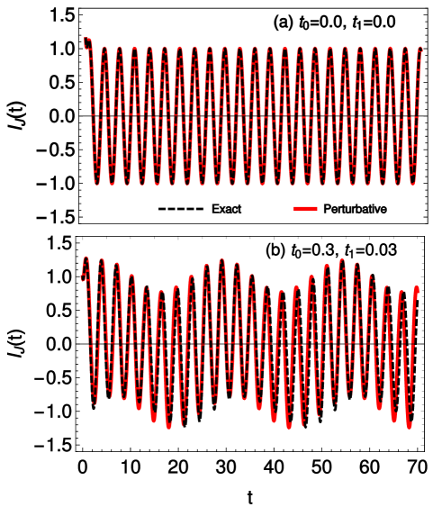
Figure 2: The variation of Josephson current with time for the setup presented in Fig. (1), i.e., the applied electric field is parallel to the charge modulation wavevector. Here we compare the exact numerical results with the analytical form of the current calculated perturbatively. (a) Shows the situation when the two orders coexist, for a vanishing $t_{0}$ and $t_{1}$. In this situation, the perturbative calculations are exact. The initial transient current regime for CDW order vanishes at a long-time limit, and we are left with the simple ac-Josephson effect. (b) Presents the Josephson current for the situation when the entanglement between the orders forms a fractionalized PDW or PDW with a finite $t_{0}=0.3,t_{1}=0.03$. The perturbative calculations and the numerical analysis shows a good match. Interestingly, the presence of entanglement between CDW and SC orders induces a beat-like modulation of the Josephson current, which can be contrasted with the simple coexistence scenario presented above.

III Results

In this section we provide the results by solving the Eqs. (12-17) and finding the Josephson current. First we discuss the terms $t_{0}$ and $t_{1}$ that generates the main difference between the two scenarios. For the simple coexistence of orders, the phase of the CDW and SC orders are not linked as discussed in the Sec. (I.2). Therefore, CDW pairs have no mechanism for having a uniform phase over the whole sample. Consequently, it suffers phase shifts and will fluctuate widely from site to site. Such an incoherent CDW pattern is expected to have minimal overlap with the SC pairs. Therefore, we can safely ignore the hopping from a PP-pair to a PH-pair, as the quantum entanglement between the orders is weak. We can set the parameters ${t_{0}=\innerproduct{\psi_{SC}^{A\left(B\right)}|\psi_{CDW}^{A\left(B\right)}}{\psi_{SC}^{A\left(B\right)}|\psi_{CDW}^{A\left(B\right)}}=0}$ and ${t_{1}=\innerproduct{\psi_{SC}^{A\left(B\right)}|\psi_{CDW}^{B\left(A\right)}}{\psi_{SC}^{A\left(B\right)}|\psi_{CDW}^{B\left(A\right)}}=0}$ in Eq.(11) for the coexistence of orders.

In the fractionalized PDW case the CDW phase $\theta^{\prime}$ is such that phase of the two electrodes is given by

$$\theta_{A}^{\prime} =\mathbf{Q}_{0}\cdot\mathbf{x}+\delta\theta_{A}^{\prime},$$

$$\theta_{B}^{\prime} =\mathbf{Q}_{0}\cdot\mathbf{\left(x+\delta\right)}+\delta\theta_{B}^{\prime},$$ (18)

where $\delta$ is a dephasing from electrode A to B. $\delta\theta_{A(B)}^{\prime}$ are the fluctuations of the phase from the initial steady state. In the setup of Fig. (1) when the electric field and wavevector $Q_{0}$ are parallel, $\delta$ is controlled by distance between the two electrodes. In Fig. (5a) we study an independent configuration, where the electric field and $Q_{0}$ are perpendicular. In such a case the dephasing is controlled by the initial the phase-shift of the CDW wavevector in the direction perpendicular to the electrodes. The main difference between the coexisting case is that now $\theta$ and $\theta^{\prime}$ are not independent. Since the phase of $\Delta_{{\rm PDW}}$ is coupled to the EM field but has $\mathbf{Q}_{0}$ modulations as well, we have

$$\theta =\delta\theta^{\prime}+\theta_{EM},$$ (19)

where $\theta_{EM}$ is the electromagnetic phase and $\delta\theta^{\prime}=\delta\theta_{B}-\delta\theta_{A}$. Assuming that we are deep inside the SC phase, with un-fractionalized Cooper pairs around, the Meissner effect leads to a uniform EM field Chakraborty et al. (2019). Thus effectively the CDW becomes active to the external EM field, due to the Meissner effect as the phase of the CDW becomes insensitive to the impurities and acts like a PDW order. Therefore a uniform CDW pattern induces inside the SC phase, an astonishing result that has been reported in Scanning Tunneling Microscopy (STM) experiment Edkins et al. (2019). Since all the phases are fixed, we now get a finite tunneling $t_{1}$ and $t_{0}$ back and forth from the modulated CDW and SC phases, and Eqs. (12-17) needs to be solved with $t,t_{0}\neq 0$.

For both the scenario, the usual Josephson current is modified due to the presence of the CDW Barone and Paterno (1982); Grüner (1988), with

$$I_{J} =-\frac{1}{2}\frac{\partial\bar{n}}{\partial t}-\frac{1}{\pi}\frac{\partial\theta^{\prime}}{\partial t}.$$ (20)

Note that the two fluids couple in the opposite way to the field – the tunneling of the charge two bosons contributes to the conventional SC Josephson current. In contrast, the variation of the phase creates a charge imbalance in the case of the CDW and generates an additional current. We solve the Eqs. (12-17) and evaluate the Josephson current by using Eq. (20). Since the difference between the two scenarions sets in at $T_{c}$, we focus on on the zero temperature limit of the Josephson current. Next we study, the alternating current (AC) Josephson effect by applying a constant potential difference between the terminals.

III.1 AC Josephson effect

III.1.1 Coexistence case

For the simple coexistence of orders since the parameters $t_{0}$ and $t_{1}$ vanishes, the Eqns. (12-17) simplifies enormously. Solving for Eq.(20) we get

$$I_{J} =\frac{2\kappa n}{\hbar}\sin\left(\frac{2\mu_{\Delta}}{\hbar}t+C_{1}\right)+\frac{C_{2}r_{0}}{\pi\hbar}e^{-r_{0}t}.$$ (21)

Here $C_{1}$ and $C_{2}$ are constants of integration and depends on the initial experimental setup. The first term in Eq.(21) is the standard AC Josephson current with the primary Josephson frequency, $\omega_{0}=(2eU)/\hbar$. Similarly, one can define standard Josephson time-period by $T=2\pi/\omega_{0}$. The second term arises due to CDW in the situation of coexisting order. Since the SC and CDW orders are disconnected, we only observe a transient response from the CDW phase variation. We have plotted the current $I_{J}$ as a function of time $t$ in Fig. (2a) for the coexistence of CDW and SC. The parameters used to obtain Fig. (2a) are given by $\mu_{\Delta}=1.0$, $n=1.0$, $n^{\prime}=1.0$, $r_{0}=3.0$, $\eta=0.3$, $\kappa=0.5$, $\kappa^{\prime}=0.6$ with $t_{1}=t_{0}=0$. We measure all the energies in the units of $2\kappa$ which we have set to unity. Furthermore, we have also set the constants $e=1$ and $\hbar=1$. We have also used the initial conditions, $\theta(t=0)=0$, $\phi(0)=0$, and $\theta^{\prime}(0)=0.6$. The transient CDW regime near $t=0$ paves the way to a standard form of the Josephson current for an standard SC current for $t\gg r_{0}$. In this situation, $I_{J}(t)$ from the numerical calculations presented in black dotted trace and the analytical form of Eq. (21) depicted in red thick trace in Fig. (2a) matches exactly.

III.1.2 Fractionalized PDW case

In the fractionalized PDW scenarion the terms $t_{0}$ and $t_{1}$ are non-vanishing. We have obtained an approximate solution of the Josephson current in Appendix (B). The Josephson current in the first order perturbation in $t_{0}$ and $t_{1}$ is given by

$$I_{J}= \frac{2\kappa n}{\hbar}\sin\left(\frac{2\mu_{\Delta}}{\hbar}t+C_{1}\right)+\frac{C_{2}r_{0}}{\pi\hbar}e^{-r_{0}t}$$

$$-\frac{2\sqrt{nn^{\prime}}}{\hbar}\cos{\frac{\phi_{0}}{2}}\left(t_{0}\sin{\frac{\theta_{0}^{\prime}-\theta_{0}}{2}}-t_{1}\sin{\frac{\theta_{0}^{\prime}+\theta_{0}}{2}}\right)$$

$$+\frac{2}{\pi\hbar}\sqrt{\frac{n^{\prime}}{n}}\sin{\frac{\phi_{0}}{2}}\left(t_{0}\sin{\frac{\theta_{0}-\theta_{0}^{\prime}}{2}}-t_{1}\sin{\frac{\theta_{0}+\theta_{0}^{\prime}}{2}}\right).$$ (22)

The time evolution of zeroth order($t_{0}=0$, $t_{1}=0$) solutions of $\theta_{0}$, $\theta_{0}^{\prime}$, and $\phi_{0}$ is given by

$$\theta_{0} =\frac{2\mu_{\Delta}}{\hbar}t+C_{1},$$ (23)

$$\theta_{0}^{\prime} =\frac{C_{2}}{\hbar}e^{-r_{0}t},$$ (24)

$$\phi_{0} =-\frac{\eta}{\hbar}t+C_{3}+\frac{2\kappa^{\prime}}{r_{0}\hbar}\text{Ci}\left[C_{2}e^{-r_{0}t}\right]-\frac{\kappa}{\mu_{\Delta}}\sin\left(\frac{2\mu_{\Delta}}{\hbar}t+C_{1}\right),$$ (25)

where again $C_{3}$ is a constant of integration and $\text{Ci}[x]$ is the cosine integral function.

We have displayed the current of Eq. (22) in Fig. (2b) for the same set of parameters as in Fig. (2a) albeit with a finite $t_{0}=0.3,t_{1}=0.03$. The perturbative analytical calculations matches well with the exact numerical form of the current. The Josephson current for the fractionalized PDW displays a beat-like structure which is strikingly distinguishable from the coexistence case. This provides us with the first prediction – If the PG phase of the underdoped cuprates supports a PDW or fractionalized PDW state, the AC Josephson current should develop a beat-like form as shown in Fig. (2b). Whereas if the orders simply coexist in the PG phase the AC Josephson current in long-times will follow the conventional form.

III.1.3 Frequency of the AC Josephson current

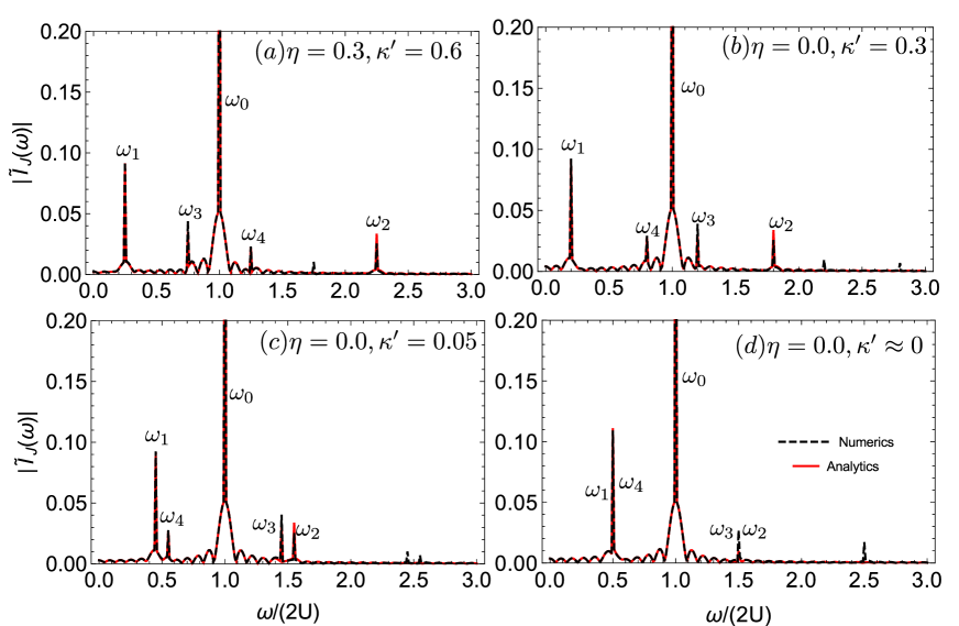
Figure 3: Exhibits the primary $\omega_{0}$ and additional frequencies $\omega_{i}$ of AC Josephson current for $t_{0}=0.3,t_{1}=0.0$. Here $\kappa^{\prime}$ and $\eta$ are material-dependent parameters. As the potential difference between the two terminals dominates the material-dependent parameters, the number of peaks reduces due to the merging of peaks as shown in (c-d). The additional peaks for $U\gg\eta+2\kappa^{\prime}$ are at the half-odd integer multiples of the primary peak $\omega_{0}$.

The Josephson current for a fractionalized PDW state shows a beat-like structure that suggests multiple frequencies contribute to the AC Josephson current. To get the frequency, we need to perform a Fourier transform of the AC Josephson current to the frequency domain.

We simplify the Eq. (22) by assuming that the inter junction PP to PH hopping amplitude is small compared to the intra-junction hoppings, i.e., $t_{1}\ll t_{0}$. In an experimental scenario, this requires using a barrier to decay the PH hoppings across the junction. However, for a finite but small $t_{1}$, will not create any qualitative difference to the discussion below. Also, in a long time limit, the transient current regime from the CDW vanishes, i.e., $\theta_{0}^{\prime}\rightarrow 0$. Following the manipulations detailed in Appendix. (C), we obtain

$$I_{J}\approx \frac{t_{0}\sqrt{nn^{\prime}}}{\hbar}\left[\mathcal{J}_{0}(b)\left\{\sin a_{+}t+\sin a_{-}t\right\}+\right.$$

$$\left.\mathcal{J}_{1}(b)\left\{\sin\left((a_{+}+\xi)t\right)-\sin\left((a_{-}+\xi)t\right)\right.\right.$$

$$\left.\left.+\sin a_{-}t-\sin a_{+}t\right\}\right]+\frac{2\kappa n}{\hbar}\sin{\xi t},$$ (26)

where $\mathcal{J}_{\nu}(x)$ is the Bessel function of first kind of the $\nu$-th order. Also we have redefined

$$a_{\pm} =\frac{1}{2}\left(\frac{2\mu_{\Delta}}{\hbar}\pm\frac{\eta}{\hbar}\pm\frac{2\kappa^{\prime}}{\hbar}\right),$$ (27)

$$b =\frac{\kappa}{2\mu_{\Delta}},$$ (28)

$$\xi =\frac{2\mu_{\Delta}}{\hbar}.$$ (29)

Since, all the terms are directly proportional to $t$, one can easily read off the frequencies for the AC current, by performing a Fourier transform. This is given by

$$\tilde{I}_{J}(\omega)= \frac{\kappa n}{\hbar}\delta({\omega-\xi})+\frac{t_{0}\sqrt{nn^{\prime}}}{2\hbar}\left[(\mathcal{J}_{0}(b)+\mathcal{J}_{1}(b))\delta(\omega-a_{-})\right.$$

$$\left.+\mathcal{J}_{1}(b)\delta(\omega-a_{+}-\xi)-\mathcal{J}_{1}(b)\delta(\omega-a_{-}-\xi)\right.$$

$$\left.+(\mathcal{J}_{0}(b)-\mathcal{J}_{1}(b))\delta(\omega-a_{-})\right].$$ (30)

The primary frequency $\xi$ is the usual AC-Josephson frequency. The other frequencies are the additional originating due to the entanglement of the two orders. The ratio of the primary to the few additional frequency is given by,

$$\frac{\omega_{1}}{\omega_{0}}=\frac{1}{2}-\left(\frac{\eta+2\kappa^{\prime}}{4eU}\right),$$ (31)

$$\frac{\omega_{4}}{\omega_{0}}=\frac{1}{2}+\left(\frac{\eta+2\kappa^{\prime}}{4eU}\right),$$ (32)

$$\frac{\omega_{2}}{\omega_{0}}=\frac{3}{2}+\left(\frac{\eta+2\kappa^{\prime}}{4eU}\right),$$ (33)

$$\frac{\omega_{3}}{\omega_{0}}=\frac{3}{2}-\left(\frac{\eta+2\kappa^{\prime}}{4eU}\right),$$ (34)

where $\omega_{i-1}$ are the $i$-th delta-function peak of Eq. (30) and used the fact that $\mu_{\Delta}=eU$, where $U$ is the DC potential applied across the terminals. For large potential difference between the two junctions, i.e., $U\gg\eta+2\kappa^{\prime}$, the second term of all the ratios vanishes. Moreover, the ratio between the primary and additional frequencies will occur at half-odd integers, i.e., $1/2,3/2,5/2,...$. However, the peak intensity will diminish for the higher-order peaks as the higher-order Bessel functions determine their strength.

We have presented in Fig. (3) the Fourier transform of the Josephson current given in Eq. (22) solved numerically in compared with the perturbative solution of Eq. (30). The dominant peaks of the AC Josephson junction are captured within our approximate analysis. The primary peak $\omega_{0}$ arising from the normal AC Josephson effect remains unchanged for all the parameters. In Fig. (3a) and Fig. (3b) when $U\sim\eta+2\kappa^{\prime}$, the four additional peaks are separated and well-resolved. The separation of the peaks $\omega_{1}$ and $\omega_{4}$ from $0.5\omega_{0}$ (similarly $\omega_{2}$ and $\omega_{3}$ from $1.5\omega_{0}$) should reduce monotonically as the potential difference between the two electrodes increases. This is illustrated in Fig. (3b) to Fig. (3d). When $U\gg\eta+2\kappa^{\prime}$, the two peaks merge as shown in Fig. (3c) and Fig. (3d) which leads to an apparent reduction in the number of peaks. Therefore when the potential difference between the terminals is large compared to the material-dependent parameters, the additional frequencies occur at half-odd integers of $\omega_{0}$. Studying such frequency dependence of the AC Josephson current peaks will give strong evidence for the fractionalized PDW scenario.

III.1.4 Envelope of the AC Josephson current

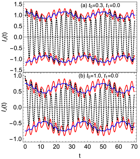
Figure 4: Presents the evolution of the beat-like form of the Josephson current for two different parameters (a) $t_{0}=0.3$, (b) $t_{0}=1$. The total envelope for the oscillation is governed by the red traces, which still contains some modulations. The blue trace shows the slower oscillation of the envelope which is controlled by the first term of Eq. (35) and hence by $\chi_{1}=(\phi_{0}-\theta_{0})/2$. This additional oscillation of the envelope is due to the entanglement between the SC and CDW order.

We have also obtained the envelope for the oscillation observed for the fractionalized PDW situation. The details for obtaining the same is presented in Appendix (D). To do this we performed a few simplifications. First, we assume that the inter junction PP to PH hopping amplitude is small compared to the intra-junction hoppings, i.e. $t_{1}\ll t_{0}$. This is not necessary a priori but it simplifies the following discussion. Experimentally, this requires hindering the $t_{1}$ hopping by using a suitable barrier. Secondly, since the envelope exists even in the long-time limit the transient response can be safely ignored. Thirdly, the expressions of current is first order perturbative solutions in $t_{0}$. We find that the expression for the current in this limit becomes,

$$I_{J}\approx \frac{n}{\hbar}\left[\sqrt{\kappa^{2}+t_{0}^{2}+2\kappa t_{0}\cos{\chi_{1}}}\right.$$

$$\left.+\sqrt{\kappa^{2}+t_{0}^{2}+2\kappa t_{0}\cos{\chi_{2}}}\right]\sin\left(\theta_{0}\right).$$ (35)

where $\chi_{1}=(\phi_{0}-\theta_{0})/2$ and $\chi_{2}=(\phi_{0}+\theta_{0})/2$.

The total envelope is shown by the red trace in Fig. (4a) and Fig. (4b) which is the term inside the square bracket in Eq. (35). The envelope term which captures the slower oscillation is exhibited by the blue traces in Fig. (4). We note that this is controlled by the $\chi_{1}$ term. Additionally, the beat-like oscillations for the fractionalized PDW becomes better resolved as the entanglement between the two order increases. Experimental observation of such dependence will also signal the fractionalized PDW in the pseudogapped phase of the underdoped cuprates.

III.1.5 Extracting modulation wavevector

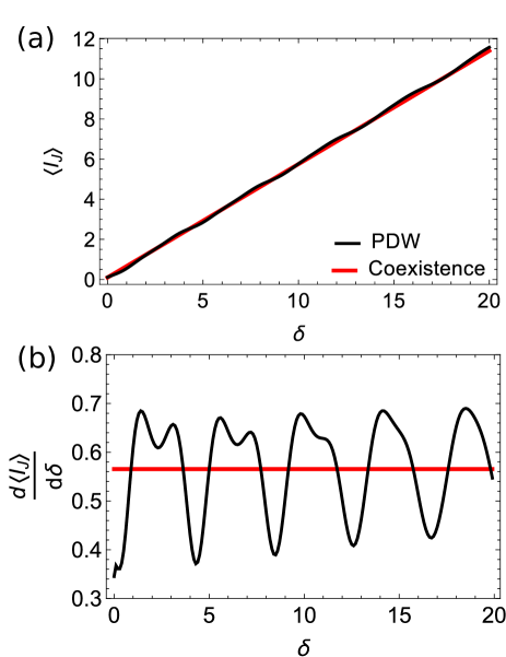
Figure 5: (a) Depicts the variation of average Josephson current with the width of the insulating region, $\delta$. The current show a linear increase for a simple coexistence of two orders, with the slope proportional to the CDW modulation wavevector. However, for a fractionalized PDW state, the Josephson current reveals a weak modulation with $\delta$. (b) Shows the derivative of the current presented in the (a). The PDW modulation wavevector $\mathbf{Q_{0}}$ controls the oscillation of the Josephson current with $\delta$, albeit higher harmonics of oscillations are also present.

It is also possible to detect the PDW modulation wavevector by varying the dephasing parameter $\delta$ between the two electrodes and by investigating its effect on the average Josephson current. The initial phases for the particle-hole pairs is given in Eq. (18), $\theta^{\prime}=Q_{0}\delta$ and $\phi=Q_{0}\delta+\gamma$, where $\gamma$ can be set to a constant. Similarly, the phase difference for the particle-particle pairs, $\theta=C_{1}$, is also a constant at $t=0$, which depends on the initial condition of the JJ setup.

We average the Josephson current, $\langle I_{J}\rangle$ using Eq. (22) over a time of 10 percent of the primary Josephson period $T$. For the coexistence of order the $\langle I_{J}\rangle$ is presented in Fig. (5a) in the red trace for $r_{0}=1.2$, $C_{1}=0$ and $Q_{0}=(1/4)2\pi/a_{0}$, where $a_{0}$ is the lattice spacing set to unity. The expression is linearly increasing with the width of the junction. The slope of the linear increase is proportional to the modulation wavevector $Q_{0}$.

However, for the fractionalized PDW scenario, along with the linear increase of the current with $\delta$, there is also weak oscillation as shown in the black trace in Fig. (5a). The modulation can be better identified by the derivative of $\langle I_{J}\rangle$ with respect to $\delta$. We depicted the same in Fig. (5b), and it shows oscillations with the primary wavelength of $2\pi/Q_{0}$. However, higher moments of oscillations make it challenging to determine the magnitude of the PDW wavevector. (for details, see Appendix (E.1)) We also note that such Josephson junction is difficult to set up in practice. In this setup, the width of the insulating region increases, which should also modify the inter-junctions hopping for different $\delta$. Moreover, fabricating JJ with varying sizes of the insulating region is challenging.

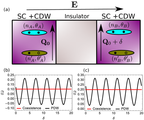
Figure 6: (a) Shows a Josephson junction setup in which the electric field is perpendicular to the charge modulation wavevector. The CDW modulations in the two terminals are dephased by a factor of $\delta$ here. (b) Depicts the evolution of the average Josephson current with the dephasing parameter $\delta$. Here the $\langle I_{J}\rangle$ is time-averaged over ten percent of the primary Josephson period. For the coexistence of orders, the average current with the dephasing parameter is constant. However, for the fractionalized PDW scenario, the Josephson current modulates with the modulation proportional to the CDW wavevector $\mathbf{Q}_{0}$. (c) The same as (b) but averaged over 20 percent of the primary Josephson period.

Next, we discuss another complementary Josephson Junction setup better suited in extracting the modulation wavevector $Q_{0}$. Fig. (6a) shows a JJ setup where the modulation wavevector is perpendicular to the electric field. Here $\delta$ denotes the phase-shift of the CDW wavevector in the B electrode with respect to the A. In this situation, $V_{A}$ and $V_{B}$ vanishes and hence $r_{0}=\eta=0$. In Fig. (6b) we plot the variation average Josephson current with $\delta$, time-averaged over $0.1$ of the usual SC Josephson period. The details of the calculations are presented in Appendix (E.2). Here, the fractionalized PDW scenario displays modulation controlled by $2\pi/Q_{0}$. In contrast, the coexistence scenario gives a flat average current with varying $\delta$. In Fig. (6c), we also establish that the modulation of the $I_{J}$ with $\delta$ remains robust when time averaging is done over twenty percent of the primary Josephson period. Therefore, in this setup, it should be possible to extract the modulation wavevector of the PDW.

III.2 Inverse Josephson effect

In the previous section, we used a constant DC-voltage $U$ across the junction, leading to an AC-Josephson current. It is also possible to apply a microwave AC-voltage to the junction, such that, $U(t)=U+\tilde{U}\cos{\omega t}$. Here $U$ is the constant DC-Voltage. Note that we have used an insulating barrier, so the normal current passing through the junction will vanish. Solving for the Josephson current, for the simple coexistence of orders, the Josephson current is given by

$$I_{J}=\frac{2\kappa n}{\hbar}\sum_{m=-\infty}^{\infty} \left[(-1)^{m}\sin\left(C_{1}+\frac{2eU}{\hbar}t-m\omega t\right)\right.$$

$$\left.\times\mathcal{J}_{m}\left(\frac{2e\tilde{U}}{\hbar\omega}\right)\right]+\frac{C_{2}r_{0}}{\pi\hbar}e^{-r_{0}t},$$ (36)

where $m$ is an integer and $\mathcal{J}_{m}$ is the Bessel function of the first kind of order $m$. The time average of this quantity gives the DC current $I_{DC}$. The long time average of the oscillatory term vanishes unless the frequency $\omega$ is some integral multiple of the applied DC-Voltage $U$ in the units where we set $(2e)/\hbar=1$. The transient current also fades away in the long time limit. The DC-current in that scenario is given by,

$$|I_{DC}|\approx\frac{2\kappa n}{\hbar}\sum_{m=-\infty}^{\infty}\delta_{m\omega,U}(-1)^{m}\mathcal{J}_{m}\left(\frac{\tilde{U}}{\omega}\right)\sin{C_{1}}$$ (37)

which leads to sharp $\delta$ peaks at the integer multiples of the AC-frequency $\omega$. These peaks are known as Shapiro spikes. We have presented the details of Shapiro Spikes in Appendix (H).

Figure 7: Demonstrates the current-voltage characteristics in the inverse Josephson setup. In (a) we set $t_{0}=0,t_{1}=0$ the parameter corresponding to the simple coexistence of CDW and SC orders. The sharp Shapiro steps can be observed when the applied DC-voltage $U$ is equal to the integer multiple of the frequency $\omega$. In (b)-(d) we plot the same for finite $t_{0},t_{1}$ which corresponds to the fractionalized PDW scenario. In (b) $t_{0},t_{1}$ is small, and other steps start developing in between the two steps. In (c)-(d) These additional steps become stronger as the entanglement between the two orders is increased and some of the integer steps vanishes completely.

Usually, in experiments, the circuit is driven by current instead of voltage. The nature of current versus voltage characteristics can be qualitatively explained from the Shapiro spikes. For instance, when the external driven current exceeds the strength of the Shapiro spike at some voltage, the voltage increases abruptly with almost zero slopes until the voltage reaches the next spike. In the subsequent level, again, as the current increases to that of the spike strength, the voltage remains stable. As the current exceeds the spike strength, the voltage again shoots up until the next spike is reached. This pattern keeps repeating itself, creating a step-like current-voltage characteristic known as Shapiro steps.

We have solved Eqns. (12-17) for an AC-voltage of the form $U(t)=U+\tilde{U}\cos{\omega t}$ and plotted the DC current as a function of the $U$ in the units where we set $(2e)/\hbar=1$ in Fig. (7). In all these figures we have used the parameters same as in Fig. (2) with AC-frequency $\omega=1$ and AC voltage amplitude $\tilde{U}=3.0$, $C_{1}=\pi/2$. We have presented the predicted current-driven nature of the current-voltage characteristics in Fig. (7). For the coexistence case, $t_{0},t_{1}=0$ and we find in Fig. (7a) the expected sharp Shapiro steps at the integer multiple of $\omega$.

Next, we solve the Eqns. (12-17) numerically for an AC-voltage of the same form but a finite $t_{0},t_{1}$ and track the evolution of the Shapiro steps. In Fig. (7b) we present the results for $t_{0}=0.1,t_{1}=0.01$, i.e., a small entanglement between the two orders leading to a weak PDW state. We find that the Shapiro steps become broader as soon as the entanglement between the two orders is turned on. New steps start to appear as the overlap between the charge and SC order increases in Fig. (7c). Finally, for a strong entanglement between the two orders, some steps appear at different DC-voltage than the integer multiple of $\omega$. Interestingly, in Fig. (7d), the first integer Shapiro step at $U=1$ is thoroughly washed away as new step-like feature forms at $U=1/2$. Therefore, our calculations suggest that additional fractional Shapiro steps in the inverse Josephson junction setup will strongly favor the PDW scenario. However, the conventional nature of voltage-current characteristics will manifest for a competing order scenario.

IV Summary and conclusions

We propose a Josephson junction setup that can distinguish between two possible scenarios which can be observed in the enigmatic pseudogap phase of the cuprates. We focused on the case of a fractionalized PDW state which can turn into interconverted SC and CDW pairs and compare this with the scenario where the SC and the CDW orders simply coexist with each other. Our findings are that in the case of a fractionalized PDW phase:

• we observe a beat-like structure of AC-Josephson current when a constant DC-Voltage is applied across the junction

• the additional frequencies for the AC Josephson current are at the half-odd integer multiple of the normal Josephson frequency for a large value of constant DC voltage.

• we can detect modulations of the Josephson current with a period proportional to the CDW wavevector $\mathbf{Q}_{0}$ by varying the dephasing parameter of the CDW modulation in two terminals.

• in the inverse Josephson setup, the induced DC-current has additional steps other than the standard integer Shapiro steps.

Identification of these signatures will strongly indicate the fractionalized PDW scenario for the pseudogap phase. Recently signatures of PDW order are seen in $\text{Bi}_{2}\text{Sr}_{2}\text{CaCu}_{2}\text{O}_{8+x}$ using a Josephson Scanning Tunnelling Microscopy setup Hamidian et al. (2016); Du et al. (2020). We, therefore, expect to observe these effects on such materials. Moreover, the predictions presented here are not dependent on the fine-tuning of material-dependent parameters.

We note that the Josephson Junction setup is shown in Fig. (1) and Fig. (6a) present just the two representative cases. For instance, in Fig. (1), the applied electric field is parallel to the modulation wavevector and in Fig. (6a), the modulation wavevector is perpendicular to the applied field. However, only short-ranged domains of unidirectional modulations are observed in cuprates Comin et al. (2015). Therefore, the samples in both terminals can contain an admixture of unidirectional domains of modulated orders. Importantly, our analysis shows that the presence of one scenario cannot critically affect the other. Consequently, we expect to discern a superposition of these two effects presented in the manuscript.

Recent studies have used Josephson scanning tunneling microscopy to observe the modulation of the Josephson current Hamidian et al. (2016); Du et al. (2020). In such studies, both the tip and sample are in the underdoped regime of the cuprates. The tips have been fabricated from the flakes of the sample itself, leading to the possible detection of the pair density wave states in cuprates. If the wavevectors of both the tip and sample align perpendicular to the applied field, the situation of Fig. (6a) will manifest. As the tip is moved parallelly over the sample, it changes the dephasing parameter $\delta$. The Josephson current modulates with the wavevector $\mathbf{Q}_{0}$ as a function of $\delta$ Hamidian et al. (2016); Du et al. (2020), very similar to our observation in Fig. (6).

Our calculations provide several predictions of the Josephson setups to detect PDW states. Any experiments that can test these features will be instrumental in differentiating between the simple coexistence of orders and the proposed pair density wave scenario.

V Acknowledgement

The authors thank Maxence Grandadam, J.C. Séamus Davis, and Yvan Sidis for valuable discussions. This work has received financial support from the ERC, under grant agreement AdG694651-CHAMPAGNE.

Appendix A The Schrödinger equations

In this section we provide complimentary details on how to derive Eq.(11). We rewrite Eq.(11) as

$$i\hbar\frac{\partial}{\partial t}\left(\sqrt{n_{A}}e^{i\theta_{A}}\right) =\mu_{\Delta}\sqrt{n_{A}}e^{i\theta_{A}}+\kappa\sqrt{n_{B}}e^{i\theta_{B}}$$ (38)

$$+t_{0}\sqrt{n_{A}^{\prime}}e^{i\theta_{A}^{\prime}}+t_{1}\sqrt{n_{A}^{\prime}}e^{i\theta_{B}^{\prime}},$$

$$i\hbar\frac{\partial}{\partial t}\left(\sqrt{n_{B}}e^{i\theta_{B}}\right) =-\mu_{\Delta}\sqrt{n_{B}}e^{i\theta_{B}}+\kappa\sqrt{n_{A}}e^{i\theta_{A}}$$ (39)

$$+t_{0}\sqrt{n_{B}^{\prime}}e^{i\theta_{B}^{\prime}}+t_{1}\sqrt{n_{A}^{\prime}}e^{i\theta_{A}^{\prime}},$$

$$i\hbar\frac{\partial}{\partial t}\left(\sqrt{n_{A}^{\prime}}e^{i\theta_{A}^{\prime}}\right) =V_{A}\sqrt{n_{A}^{\prime}}e^{i\theta_{A}^{\prime}}+\kappa^{\prime}\sqrt{n_{B}^{\prime}}e^{i\theta_{B}^{\prime}}$$ (40)

$$+t_{0}\sqrt{n_{A}}e^{i\theta_{A}}+t_{1}\sqrt{n_{B}}e^{i\theta_{B}},$$

$$i\hbar\frac{\partial}{\partial t}\left(\sqrt{n_{B}^{\prime}}e^{i\theta_{B}^{\prime}}\right) =V_{B}\sqrt{n_{B}^{\prime}}e^{i\theta_{B}^{\prime}}+\kappa^{\prime}\sqrt{n_{A}^{\prime}}e^{i\theta_{A}^{\prime}}$$ (41)

$$+t_{0}\sqrt{n_{B}}e^{i\theta_{B}}+t_{1}\sqrt{n_{A}}e^{i\theta_{A}}.$$

Expanding Eq.(38) and taking the complex conjugate of it yields

$$i\hbar\left(\dot{\sqrt{n_{A}}}+i\dot{\theta}_{A}\sqrt{n_{A}}\right)e^{i\theta_{A}} =\mu_{\Delta}\sqrt{n_{A}}e^{i\theta_{A}}+\kappa\sqrt{n_{B}}e^{i\theta_{B}}$$

$$+t_{0}\sqrt{n_{A}^{\prime}}e^{i\theta_{A}^{\prime}}+t_{1}\sqrt{n_{A}^{\prime}}e^{i\theta_{B}^{\prime}},$$ (42)

$$-i\hbar\left(\dot{\sqrt{n_{A}}}-i\dot{\theta}_{A}\sqrt{n_{A}}\right)e^{-i\theta_{A}} =\mu_{\Delta}\sqrt{n_{A}}e^{-i\theta_{A}}+\kappa\sqrt{n_{B}}e^{-i\theta_{B}}$$

$$+t_{0}\sqrt{n_{A}^{\prime}}e^{-i\theta_{A}^{\prime}}+t_{1}\sqrt{n_{A}^{\prime}}e^{-i\theta_{B}^{\prime}}.$$ (43)

Adding Eqs.(42) and (43) leads to

$$\frac{\partial n_{A}}{\partial t}=\frac{2}{\hbar} \left[\kappa\sqrt{n_{A}n_{B}}\sin\theta+t_{0}\sqrt{n_{A}n_{A}^{\prime}}\sin(\theta_{A}^{\prime}-\theta_{A})\right.$$

$$\left.+t_{1}\sqrt{n_{B}^{\prime}n_{A}}\sin(\theta_{B}^{\prime}-\theta_{A})\right],$$ (44)

where $\theta=\theta_{B}-\theta_{A}$. Next subtracting Eq. (42) from Eq. (43) leads to

$$\frac{\partial\theta_{A}}{\partial t}=-\frac{1}{\hbar} \left[\mu_{\Delta}+\kappa\sqrt{\frac{n_{B}}{n_{A}}}\cos\theta+t_{0}\sqrt{\frac{n_{A}^{\prime}}{n_{A}}}\cos(\theta_{A}^{\prime}-\theta_{A})\right.$$

$$\left.+t_{1}\sqrt{\frac{n_{B}^{\prime}}{n_{A}}}\cos(\theta_{B}^{\prime}-\theta_{A})\right],$$ (45)

Next repeating the same procedure for the Eq. (39), we obtain the corresponding equations for $n_{B}$ and $\theta_{B}$ as follows,

$$\frac{\partial n_{B}}{\partial t}=\frac{2}{\hbar} \left[-\kappa\sqrt{n_{A}n_{B}}\sin\theta+t_{0}\sqrt{n_{B}n_{B}^{\prime}}\sin(\theta_{B}^{\prime}-\theta_{B})\right.$$

$$\left.+t_{1}\sqrt{n_{A}^{\prime}n_{B}}\sin(\theta_{A}^{\prime}-\theta_{B})\right],$$ (46)

$$\frac{\partial\theta_{B}}{\partial t}=\frac{1}{\hbar} \left[\mu_{\Delta}-\kappa\sqrt{\frac{n_{A}}{n_{B}}}\cos\theta-t_{0}\sqrt{\frac{n_{B}^{\prime}}{n_{B}}}\cos(\theta_{B}^{\prime}-\theta_{B})\right.$$

$$\left.-t_{1}\sqrt{\frac{n_{A}^{\prime}}{n_{B}}}\cos(\theta_{A}^{\prime}-\theta_{B})\right].$$ (47)

We define $\bar{n}=n_{B}-n_{A}$, subtracting Eq. (44) from Eq. (46), lead to

$$\frac{\partial\bar{n}}{\partial t} =\frac{2}{\hbar}\left[-2\kappa\sqrt{n_{A}n_{B}}\sin\theta\right.$$

$$\left.+t_{0}\left(\sqrt{n_{B}n_{B}^{\prime}}\sin(\theta_{B}^{\prime}-\theta_{B})-\sqrt{n_{A}n_{A}^{\prime}}\sin(\theta_{A}^{\prime}-\theta_{A})\right)\right.$$

$$\left.+t_{1}\left(\sqrt{n_{A}^{\prime}n_{B}}\sin(\theta_{A}^{\prime}-\theta_{B})-\sqrt{n_{B}^{\prime}n_{A}}\sin(\theta_{B}^{\prime}-\theta_{A})\right)\right].$$ (48)

Approximating, that the density of of particle-particle pairs and particle-hole pairs in both the terminals is similar in the steady state, i.e., $n_{A}\approx n_{B}=n$ and $n_{A}^{\prime}\approx n_{B}^{\prime}=n^{\prime}$ and defining $\phi=\theta_{A}^{\prime}+\theta_{B}^{\prime}-\theta_{A}-\theta_{B}$, we obtain

$$\frac{\partial\bar{n}}{\partial t}=\frac{4}{\hbar} \left[-\kappa n\sin{\theta}+\sqrt{nn^{\prime}}\cos{\frac{\phi}{2}}\right.$$

$$\left.\times\left(t_{0}\sin{\frac{\theta^{\prime}-\theta}{2}}-t_{1}\sin{\frac{\theta^{\prime}+\theta}{2}}\right)\right],$$ (49)

where $\theta^{\prime}=\theta_{B}^{\prime}-\theta_{A}^{\prime}$. Following the same procedure and approximation we can obtain the differential equation for $\theta$, which is given by

$$\frac{\partial\theta}{\partial t}=\frac{2}{\hbar} \left[\mu_{\Delta}+\sqrt{\frac{n^{\prime}}{n}}\sin{\frac{\phi}{2}}\right.$$

$$\left.\times\left(t_{0}\sin{\frac{\theta^{\prime}-\theta}{2}}-t_{1}\sin{\frac{\theta+\theta^{\prime}}{2}}\right)\right],$$ (50)

Repeating the procedure for Eqs. (40), (41), we obtain the differential equation for the $\bar{n}^{\prime}$ and $\theta^{\prime}$.

$$\frac{\partial\bar{n}^{\prime}}{\partial t}=\frac{4}{\hbar} \left[-\kappa^{\prime}n^{\prime}\sin{\theta^{\prime}}+\sqrt{nn^{\prime}}\cos{\frac{\phi}{2}}\right.$$

$$\left.\times\left(t_{0}\sin{\frac{\theta-\theta^{\prime}}{2}}-t_{1}\sin{\frac{\theta^{\prime}+\theta}{2}}\right)\right],$$ (51)

$$\frac{\partial\theta^{\prime}}{\partial t}=\frac{1}{\hbar} \left[(V_{A}-V_{B})-2\sqrt{\frac{n^{\prime}}{n}}\sin{\frac{\phi}{2}}\right.$$

$$\left.\times\left(t_{0}\sin{\frac{\theta-\theta^{\prime}}{2}}-t_{1}\sin{\frac{\theta^{\prime}+\theta}{2}}\right)\right],$$ (52)

Using all these forms for the $\theta$’s we can obtain the time evolution equation for the $\phi$

$$\frac{\partial\phi}{\partial t}= -\frac{1}{\hbar}\left[(V_{A}+V_{B})+2\kappa\cos{\theta}+2\kappa^{\prime}\cos{\theta^{\prime}}\right.$$

$$\left.-\frac{2(n-n^{\prime})}{\sqrt{nn^{\prime}}}\left(t_{0}\cos{\frac{\theta-\theta^{\prime}}{2}}+t_{1}\cos{\frac{\theta+\theta^{\prime}}{2}}\right)\right],$$ (53)

The fourth term on the RHS can be approximately taken to be small when the particle-particle pairs and the particle-hole pairs are of similar strength, i,e, $\delta n/n\ll 1$ and thus we obtain

$$\frac{\partial\phi}{\partial t}\approx -\frac{1}{\hbar}\left[(V_{A}+V_{B})+2\kappa\cos{\theta}+2\kappa^{\prime}\cos{\theta^{\prime}}\right].$$ (54)

We need to solve the five coupled differential Eqns. (49), (50), (51), (52), and (54).

Appendix B Evaluation of Josephson current

The Josephson current is obtained by the expression Barone and Paterno (1982); Grüner (1988)

$$I_{J}=-\frac{1}{2}\frac{\partial\bar{n}}{\partial t}-\frac{1}{\pi}\frac{\partial\theta^{\prime}}{\partial t}.$$ (55)

To find this, we need a solution to the equations presented in the previous section. Using the forms for the difference of potential between the two terminal due to charge density modulations as $V_{A}-V_{B}=-eE\bar{\rho}\theta^{\prime}\equiv-r_{0}\theta^{\prime}$, with the average of the same $V_{A}+V_{B}=\eta$ set to constant. The coupled differential equations can be written in a condensed form as,

$$\frac{\partial\bar{n}}{\partial t} =\frac{4}{\hbar}\left[-\kappa n\sin{\theta}+\sqrt{nn^{\prime}}\cos{\frac{\phi}{2}}f(t_{0},t_{1},\theta,\theta^{\prime})\right],$$ (56)

$$\frac{\partial\theta}{\partial t} =\frac{2}{\hbar}\left[\mu_{\Delta}+\sqrt{\frac{n^{\prime}}{n}}\sin{\frac{\phi}{2}}f(t_{0},t_{1},\theta,\theta^{\prime})\right],$$ (57)

$$\frac{\partial\bar{n}^{\prime}}{\partial t} =\frac{4}{\hbar}\left[-\kappa^{\prime}n^{\prime}\sin{\theta^{\prime}}+\sqrt{nn^{\prime}}\cos{\frac{\phi}{2}}g(t_{0},t_{1},\theta,\theta^{\prime})\right],$$ (58)

$$\frac{\partial\theta^{\prime}}{\partial t} =\frac{1}{\hbar}\left[-r_{0}\theta^{\prime}-2\sqrt{\frac{n^{\prime}}{n}}\sin{\frac{\phi}{2}}g(t_{0},t_{1},\theta,\theta^{\prime})\right],$$ (59)

$$\frac{\partial\phi}{\partial t} =-\frac{1}{\hbar}\left[\eta+2\kappa\cos{\theta}+2\kappa^{\prime}\cos{\theta^{\prime}}\right].$$ (60)

Here we have defined,

$$f(t_{0},t_{1},\theta,\theta^{\prime})=\left(t_{0}\sin{\frac{\theta^{\prime}-\theta}{2}}-t_{1}\sin{\frac{\theta^{\prime}+\theta}{2}}\right),$$ (61)

$$g(t_{0},t_{1},\theta,\theta^{\prime})=\left(t_{0}\sin{\frac{\theta-\theta^{\prime}}{2}}-t_{1}\sin{\frac{\theta+\theta^{\prime}}{2}}\right).$$ (62)

These equations can be solved using numerical means for any parameter, and Josephson current can be evaluated using Eq. (55). However, here we discuss an approach to calculate when the $t_{0}$ and $t_{1}$ are small parameters that can be incorporated perturbatively in the expression. In this approach, we expand the solutions

$$\bar{n} =\bar{n}_{0}+(t_{0}+t_{1})\bar{n}_{1}+(t_{0}+t_{1})^{2}\bar{n}_{2}+...$$ (63)

$$\theta^{\prime} =\theta_{0}^{\prime}+(t_{0}+t_{1})\theta_{1}^{\prime}+(t_{0}+t_{1})^{2}\theta_{2}^{\prime}+...$$ (64)

and so on for other variables, and the subscript represents the perturbative order of the solution. The zeroth-order solution is readily obtained by putting $t_{0}=0$ and $t_{1}=0$ in Eq. (56) to Eq. (60). The relevant equations becomes,

$$\frac{\partial\bar{n}_{0}}{\partial t} =-\frac{4\kappa n}{\hbar}\sin{\theta_{0}},$$ (65)

$$\frac{\partial\theta_{0}}{\partial t} =\frac{2\mu_{\Delta}}{\hbar},$$ (66)

$$\frac{\partial\theta_{0}^{\prime}}{\partial t} =-\frac{r_{0}}{\hbar}\theta_{0}^{\prime},$$ (67)

$$\frac{\partial\phi_{0}}{\partial t} =-\frac{1}{\hbar}\left[\eta+2\kappa\cos{\theta_{0}}+2\kappa^{\prime}\cos{\theta_{0}^{\prime}}\right].$$ (68)

The solution for these equations are readily obtained and these are given by,

$$\theta_{0} =\frac{2\mu_{\Delta}}{\hbar}t+C_{1},$$ (69)

$$\theta_{0}^{\prime} =\frac{C_{2}}{\hbar}e^{-r_{0}t},$$ (70)

and the zeroth order Josephson current becomes,

$$I_{J}^{(0)}=\frac{2\kappa n}{\hbar}\sin\left(\frac{2\mu_{\Delta}}{\hbar}t+C_{1}\right)+\frac{C_{2}r_{0}}{\pi\hbar}e^{-r_{0}t},$$ (71)

where $C_{1}$ and $C_{2}$ are the constants of integration. Notice that the first term is the usual Josephson current for a superconducting junction, whereas the second term is a transient current due to the presence of charge orders. When the entanglement between the orders are small, i.e. for a simple coexistence of order Eq. (71) gives the exact form of the current.

Next we focus on obtaining the first order correction to this current. To this end, we need the zeroth order expression for $\phi_{0}$, which can be obtained by using $\theta_{0}$ and $\theta_{0}^{\prime}$ in Eq. (68),

$$\phi_{0}=-\frac{\eta}{\hbar}t+C_{3}+\frac{2\kappa^{\prime}}{r_{0}\hbar}\text{Ci}\left[C_{2}e^{-r_{0}t}\right]-\frac{\kappa}{\mu_{\Delta}}\sin\left(\frac{2\mu_{\Delta}}{\hbar}t+C_{1}\right),$$ (72)

where again $C_{3}$ is a constant of integration and $\text{Ci}[x]$ is the cosine integral function. The first order, equations can now be evaluated by taking the derivative of Eq. (56) and Eq. (59) with respect to $t_{0}$ and $t_{1}$ individually and subsequently setting these small parameter to zero. Therefore the first-order correction for the terms relevant for the Josephson current thus becomes

$$\frac{\partial\bar{n}_{1}}{\partial t} =\frac{4\sqrt{nn^{\prime}}}{\hbar}\cos{\frac{\phi_{0}}{2}}\left(t_{0}\sin{\frac{\theta_{0}^{\prime}-\theta_{0}}{2}}-t_{1}\sin{\frac{\theta_{0}^{\prime}+\theta_{0}}{2}}\right),$$ (73)

$$\frac{\partial\theta_{1}^{\prime}}{\partial t} =-\frac{2}{\hbar}\sqrt{\frac{n^{\prime}}{n}}\sin{\frac{\phi_{0}}{2}}\left(t_{0}\sin{\frac{\theta-\theta_{0}^{\prime}}{2}}-t_{1}\sin{\frac{\theta_{0}+\theta_{0}^{\prime}}{2}}\right).$$ (74)

Therefore up to the first order the Josephson current is given by,

$$I_{J}= \frac{2\kappa n}{\hbar}\sin\left(\frac{2\mu_{\Delta}}{\hbar}t+C_{1}\right)+\frac{C_{2}r_{0}}{\pi\hbar}e^{-r_{0}t}$$

$$-\frac{2\sqrt{nn^{\prime}}}{\hbar}\cos{\frac{\phi_{0}}{2}}\left(t_{0}\sin{\frac{\theta_{0}^{\prime}-\theta_{0}}{2}}-t_{1}\sin{\frac{\theta_{0}^{\prime}+\theta_{0}}{2}}\right)$$

$$+\frac{2}{\pi\hbar}\sqrt{\frac{n^{\prime}}{n}}\sin{\frac{\phi_{0}}{2}}\left(t_{0}\sin{\frac{\theta_{0}-\theta_{0}^{\prime}}{2}}-t_{1}\sin{\frac{\theta_{0}+\theta_{0}^{\prime}}{2}}\right),$$ (75)

where we can use the time evolution of $\theta_{0}$, $\theta_{0}^{\prime}$, and $\phi_{0}$ from Eq. (69), Eq. (70) and Eq. (72) respectively. In the main text, this form is compared favorably with the exact current evaluated by solving the equations numerically.

Appendix C Extracting the frequencies of the AC Josephson current

The Josephson current for a fractionalized PDW state shows a beat like structure. This suggests multiple frequencies are contributing to the AC Josephson current. This section provides the details to obtain the Josephson current frequencies. To do so, we need to perform a Fourier transform of the AC Josephson current to the frequency domain.

We simplify the Eq. (75) by assuming that the inter junction PP to PH hopping amplitude is small compared to the intra-junction hoppings, i.e., $t_{1}\ll t_{0}$. In an experimental scenario, this requires using a barrier to decay the PH hoppings across the junction. However, for a finite but small $t_{1}$, will not create any qualitative difference to the discussion below. Also, in a long time limit, the transient current regime from the CDW vanishes, i.e., $\theta_{0}^{\prime}\rightarrow 0$. Hence the current reduces to

$$I_{J}\approx \frac{2\kappa n}{\hbar}\sin{\theta_{0}}+\frac{2t_{0}\sqrt{nn^{\prime}}}{\hbar}\cos{\frac{\phi_{0}}{2}}\sin{\frac{\theta_{0}}{2}}$$

$$-\frac{2t_{0}}{\pi\hbar}\sqrt{\frac{n^{\prime}}{n}}\sin{\frac{\phi_{0}}{2}}\sin{\frac{\theta_{0}}{2}},$$ (76)

Furthermore, since the $n\approx n^{\prime}$, the second term dominates over the third. The expression for the current further simplifies to

$$I_{J}\approx \frac{2\kappa n}{\hbar}\sin{\theta_{0}}+\frac{2t_{0}\sqrt{nn^{\prime}}}{\hbar}\cos{\frac{\phi_{0}}{2}}\sin{\frac{\theta_{0}}{2}}.$$ (77)

Using trignometric identities, the second term becomes,

$$I_{2}\approx \frac{t_{0}\sqrt{nn^{\prime}}}{\hbar}\left[\sin\left(\frac{\theta_{0}+\phi_{0}}{2}\right)+\sin\left(\frac{\theta_{0}-\phi_{0}}{2}\right)\right].$$ (78)

The $\theta_{0}$ and $\phi_{0}$ is given by Eq. (69) and Eq. (72) respectively. The constant terms do not contribute to the frequency of the AC Josephson frequency, and hence we can ignore them for the following analysis. Next we make a series expansion for $Ci[...]$ function and neglecting the constant and higer order terms, we obtain

$$I_{2}\approx \frac{t_{0}\sqrt{nn^{\prime}}}{\hbar}\left[\sin\left(a_{+}+b\sin{\xi t}\right)+\sin\left(a_{-}-b\sin{\xi t}\right)\right],$$ (79)

where we have defined

$$a_{\pm} =\frac{1}{2}\left(\frac{2\mu_{\Delta}}{\hbar}\pm\frac{\eta}{\hbar}\pm\frac{2\kappa^{\prime}}{\hbar}\right)$$ (80)

$$b =\frac{\kappa}{2\mu_{\Delta}}$$ (81)

$$\xi =\frac{2\mu_{\Delta}}{\hbar}$$ (82)

Next, we expand

$$\cos(x\sin\theta)=\mathcal{J}_{0}(x)+2\sum_{p=1}^{\infty}\mathcal{J}_{2p}(x)\cos(2p\theta),$$ (83)

$$\sin(x\sin\theta)=2\sum_{p=1}^{\infty}\mathcal{J}_{2p+1}(x)\sin((2p+1)\theta),$$ (84)

Where $\mathcal{J}_{\nu}(x)$ is the Bessel function of first kind of the $\nu$-th order. Neglecting the higher order terms the current in Eq. (76) becomes

$$I_{J}\approx \frac{t_{0}\sqrt{nn^{\prime}}}{\hbar}\left[\mathcal{J}_{0}(b)\left\{\sin a_{+}t+\sin a_{-}t\right\}+\right.$$

$$\left.\mathcal{J}_{1}(b)\left\{\sin\left((a_{+}+\xi)t\right)-\sin\left((a_{-}+\xi)t\right)\right.\right.$$

$$\left.\left.+\sin a_{-}t-\sin a_{+}t\right\}\right]+\frac{2\kappa n}{\hbar}\sin{\xi t}$$ (85)

Since, all the terms are directly proportional to $t$, one can easily read off the frequencies for the AC current, by performing a fourier transform. This is given by

$$\tilde{I}_{J}(\omega)= \frac{\kappa n}{\hbar}\delta({\omega-\xi})+\frac{t_{0}\sqrt{nn^{\prime}}}{2\hbar}\left[(\mathcal{J}_{0}(b)+\mathcal{J}_{1}(b))\delta(\omega-a_{-})\right.$$

$$\left.+\mathcal{J}_{1}(b)\delta(\omega-a_{+}-\xi)-\mathcal{J}_{1}(b)\delta(\omega-a_{-}-\xi)\right.$$

$$\left.+(\mathcal{J}_{0}(b)-\mathcal{J}_{1}(b))\delta(\omega-a_{-})\right]$$ (86)

The primary frequency $\xi$ is the usual AC Josephson frequency. The other frequencies are the additional ones originating due to the entanglement of the two orders. The ratio of the primary to the few additional frequencies is given by,

$$\frac{\omega_{1}}{\omega_{0}}=\frac{1}{2}-\left(\frac{\eta+2\kappa^{\prime}}{4eU}\right),$$ (87)

$$\frac{\omega_{4}}{\omega_{0}}=\frac{1}{2}+\left(\frac{\eta+2\kappa^{\prime}}{4eU}\right),$$ (88)

$$\frac{\omega_{2}}{\omega_{0}}=\frac{3}{2}+\left(\frac{\eta+2\kappa^{\prime}}{4eU}\right),$$ (89)

$$\frac{\omega_{3}}{\omega_{0}}=\frac{3}{2}-\left(\frac{\eta+2\kappa^{\prime}}{4eU}\right),$$ (90)

where $\omega_{i-1}$ are the $i$-th delta function peak of Eq. (86). For large potential difference between the two junctions i.e., $U\gg\eta+2\kappa^{\prime}$, the second term of all the ratios vanish. Moreover, the ratio between the primary and additional frequencies will occur at half-odd integers, i.e., $1/2,3/2,5/2,...$. However, the peak strength will diminish for the higher order term as it is determined by the higher order Bessel function. Studying such frequency dependence of the AC Josephson current will give an indication of the fractionalized PDW order.

Appendix D Extracting the envelope

The Josephson current for a PDW state or fractionalized PDW state shows a beat like structure. Such a beat-like form can be distinguished in experiments establishing an entanglement between the superconducting and the charge orders. To provide a detailed description, it becomes necessary to determine the parameters that control such a current envelope. In this section, we provide the details of the envelope of the Josephson current. We start with Eq.(77) Using trignometric identities, we obtain

$$I_{J}= \frac{\kappa n}{\hbar}\sin{\theta_{0}}+\frac{t_{0}\sqrt{nn^{\prime}}}{\hbar}\sin\left(\theta_{0}+\frac{\phi_{0}-\theta_{0}}{2}\right)$$

$$+\frac{\kappa n}{\hbar}\sin{\theta_{0}}+\frac{t_{0}\sqrt{nn^{\prime}}}{\hbar}\sin\left(\theta_{0}-\frac{\phi_{0}+\theta_{0}}{2}\right).$$ (91)

Before adding the sine waves we define, $(\phi_{0}-\theta_{0})/2=\chi_{1}$ and $(\phi_{0}+\theta_{0})/2=\chi_{2}$. Therefore, using $n\approx n^{\prime}$, the expression current becomes,

$$I_{J}= \frac{n}{\hbar}\left[\sqrt{\kappa^{2}+t_{0}^{2}+2\kappa t_{0}\cos{\chi_{1}}}\sin\left(\theta_{0}+\xi_{1}\right)\right.$$

$$\left.+\sqrt{\kappa^{2}+t_{0}^{2}+2\kappa t_{0}\cos{\chi_{2}}}\sin\left(\theta_{0}-\xi_{2}\right)\right].$$ (92)

Here the phase angles $\xi_{i}$ are given by

$$\xi_{i}=\sin^{-1}\left(\frac{t_{0}\sin{\chi_{i}}}{\sqrt{\kappa^{2}+t_{0}^{2}+2\kappa t_{0}\cos{\chi_{i}}}}\right),$$ (93)

where $i=1,2$. In the perturbative limit, $t_{0}$ is the small parameter in our calculations, the phase shifts can be assumed to be small, such that $\xi_{i}=0$. Therefore the current becomes

$$I_{J}= \frac{n}{\hbar}\sum_{i=1}^{2}\left[\sqrt{\kappa^{2}+t_{0}^{2}+2\kappa t_{0}\cos{\chi_{i}}}\right]\sin\left(\theta_{0}\right).$$ (94)

Here the amplitude of the envelope is controlled by two phases. The faster oscillation is governed by $\chi_{2}=(\phi_{0}+\theta_{0})/2$ and the slower one by $\chi_{1}=(\phi_{0}-\theta_{0})/2$. The total envelope is the sum of the square root term in Eq. (94), and therefore contains further oscillations given by $\chi_{1}$ and $\chi_{2}$.

Appendix E Josephson current with dephasing parameter

E.1 Electric field parallel to $\mathbf{Q_{0}}$

This appendix discusses the procedure to obtain the average Josephson current with the dephasing parameter. Initially at $t=0$, the phase of the CDW order is given by $\theta^{\prime}(0)=Q_{0}\delta=C_{2}$. Similarly, one can set $\phi(0)=Q_{0}\delta+\gamma$, where $\gamma$ is a constant. The zeroth order solution for $\phi$, thus becomes

$$\phi_{0}=-\frac{\eta}{\hbar}t+(Q_{0}\delta+\gamma)+\frac{2\kappa^{\prime}}{r_{0}\hbar}\text{Ci}\left[Q_{0}\delta e^{-r_{0}t}\right]$$

$$-\frac{\kappa}{\mu_{\Delta}}\sin\left(\frac{2\mu_{\Delta}}{\hbar}t+C_{1}\right).$$ (95)

Putting this in Eq. (22), we obtain the $I_{J}(t)$, which we integrate numerically over a fixed time to get the average $\langle I_{J}\rangle$. Notice, the cosine-integral dependence of $\delta$ in $\phi_{0}$ generates a higher harmonics of oscillation of $\langle I_{J}\rangle$ with $\delta$. Thus, it becomes difficult to extract the PDW modulation wavevector in this setup.

E.2 Electric field perpendicular to $\mathbf{Q_{0}}$

No such complications arise when the JJ is set up is such that the wavevector is perpendicular to the electric field. In this case, although $r_{0}=\eta=0$ and the transient current cannot survive, yet initial $\theta_{0}^{\prime}(0)=Q_{0}\delta$. Similarly, one can set $\phi(0)=Q_{0}\delta+\gamma$, where $\gamma$ is a constant. Here $\delta$ denotes the phase difference between the CDW wavevector in the two terminals. Consequently, the zeroth-order solutions become

$$\theta_{0} =\frac{2\mu_{\Delta}}{\hbar}t+C_{1},$$ (96)

$$\theta_{0}^{\prime} =Q_{0}\delta,$$ (97)

$$\phi_{0} =(Q_{0}\delta+\gamma)-\frac{2\kappa^{\prime}}{\hbar}\cos\left(Q_{0}\delta\right)t-\frac{\kappa}{\mu_{\Delta}}\sin\left(\frac{2\mu_{\Delta}}{\hbar}t+C_{1}\right).$$ (98)

Putting these expressions in the Eq. (22), we can evaluate average current, which shows clear modulations with $\delta$.

Appendix F Current due to CDW phase

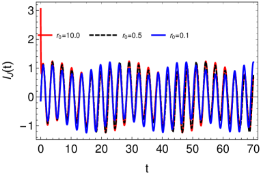
Figure 8: Shows the AC Josephson current for different values of $r_{0}$. The beat-like structure for the AC current remains robust for all the values of $r_{0}$. Only the intial transient nature of the current vanishes for smaller $r_{0}$.

The CDW phase can be strongly pinned by the boundary of the junctions and the disorder of the samples. However, here we consider the general possibility for the current arising due to the phase of the CDW order. We note that the term ${V_{A}-V_{B}=-(eEn^{\prime}/Q_{0})\theta^{\prime}\equiv-r_{0}\theta^{\prime}}$, generates only a transient current response at short times. The parameter $r_{0}$ characterizes the strength of the phase current from the CDW. The long-time behavior of the AC Josephson current remains invariant when we vary this term. In Fig. (8), we have shown the evolution of AC Josephson current for the PDW scenario. The parameters used here are the same as those presented in Fig. (2b) of the main text. As we increase the $r_{0}$, the AC response changes for $t\rightarrow 0$, whereas it remains invariant at long times. The frequency of the oscillation is independent of $r_{0}$ and thus remains the same. The amplitude of the oscillation changes weakly when $r_{0}<1$. Therefore, the results presented in the manuscript remain robust while we change this parameter.

Appendix G Josephson current with complex hoppings

Here we consider the complex hoppings between the particle-particle to particle-hole hoppings. Since this term is connected by the PDW order, it can be complex in general. We confirm here whether the imaginary part of these hoppings consideribly modifies our results.

The set of Schrödinger’s equations write, with $\overline{\psi}=\left(\begin{array}[]{cccc}\sqrt{n_{A}}e^{i\theta_{A}},&\sqrt{n_{B}}e^{i\theta_{B}},&\sqrt{n_{A}^{\prime}}e^{i\theta_{A}^{\prime}},&\sqrt{n_{B}^{\prime}}e^{i\theta_{B}^{\prime}}\end{array}\right)$

$$i\hbar\frac{\partial}{\partial t}\psi =\left(\begin{array}[]{cccc}\mu_{\Delta}&\kappa&t_{0}&t_{1}\\ \kappa&-\mu_{\Delta}&t_{1}&t_{0}\\ t_{0}^{*}&t_{1}^{*}&V_{A}&\kappa^{\prime}\\ t_{1}^{*}&t_{0}^{*}&\kappa^{\prime}&V_{B}\end{array}\right)\psi,$$ (103)

By following the pocedure similar to Appendix. (A), we arrive at the set of Schrödinger equations

$$\frac{\partial\bar{n}}{\partial t} =\frac{4}{\hbar}\left[-\kappa n\sin\theta+\sqrt{nn^{\prime}}\left\{\cos\frac{\phi}{2}\left(\text{Re }t_{0}\sin{\frac{\theta^{\prime}-\theta}{2}}-\text{Re }t_{1}\sin{\frac{\theta^{\prime}+\theta}{2}}\right)-\sin\frac{\phi}{2}\left(\text{Im }t_{0}\sin{\frac{\theta^{\prime}-\theta}{2}}-\text{Im }t_{1}\sin{\frac{\theta^{\prime}+\theta}{2}}\right)\right\}\right],$$ (104)

$$\frac{\partial\theta}{\partial t} =\frac{2}{\hbar}\left[\mu_{\Delta}+\sqrt{\frac{n^{\prime}}{n}}\left\{\sin\frac{\phi}{2}\left(\text{Re }t_{0}\sin{\frac{\theta^{\prime}-\theta}{2}}-\text{Re }t_{1}\sin{\frac{\theta^{\prime}+\theta}{2}}\right)-\cos\frac{\phi}{2}\left(\text{Im }t_{0}\sin{\frac{\theta^{\prime}-\theta}{2}}-\text{Im }t_{1}\sin{\frac{\theta^{\prime}+\theta}{2}}\right)\right\}\right],$$ (105)

$$\frac{\partial\bar{n}^{\prime}}{\partial t} =\frac{4}{\hbar}\left[-\kappa^{\prime}n^{\prime}\sin\theta^{\prime}+\sqrt{nn^{\prime}}\left\{\cos\frac{\phi}{2}\left(\text{Re }t_{0}\sin{\frac{\theta-\theta^{\prime}}{2}}-\text{Re }t_{1}\sin{\frac{\theta^{\prime}+\theta}{2}}\right)-\sin\frac{\phi}{2}\left(\text{Im }t_{0}\sin{\frac{\theta-\theta^{\prime}}{2}}-\text{Im }t_{1}\sin{\frac{\theta^{\prime}+\theta}{2}}\right)\right\}\right],$$ (106)

$$\frac{\partial\theta^{\prime}}{\partial t} =\frac{1}{\hbar}\left[V_{A}-V_{B}-2\sqrt{\frac{n}{n^{\prime}}}\left\{\sin\frac{\phi}{2}\left(\text{Re }t_{0}\sin{\frac{\theta-\theta^{\prime}}{2}}-\text{Re }t_{1}\sin{\frac{\theta^{\prime}+\theta}{2}}\right)-\cos\frac{\phi}{2}\left(\text{Im }t_{0}\sin{\frac{\theta-\theta^{\prime}}{2}}-\text{Im }t_{1}\sin{\frac{\theta^{\prime}+\theta}{2}}\right)\right\}\right],$$ (107)

$$\frac{\partial\phi}{\partial t} =-\frac{1}{\hbar}\left[\eta+2\kappa\cos{\theta}+2\kappa^{\prime}\cos{\theta^{\prime}}\right].$$ (108)

We solve the equations numerically and derive the Josephson current using Eq.(20). The results are presented in Fig. (9).

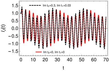
Figure 9: AC Josephson current for two scenarios. In both the $\text{Re }t_{0}=0.3$ and $\text{Re }t_{1}=0.03$. Moreover, all other parameters are the same as we used in Fig. (2b). The dashed lines manifest the effects of the imaginary part of the $t_{0}$, and $t_{1}$ is finite. Although the amplitude of the current changes slightly as we increase the imaginary part of the hoppings, the oscillation frequencies remain the same.

It shows the Josephson current as the imaginary part of the hoppings are increased. Although the amplitude of the current changes with the increasing imaginary part of the hoppings, the frequency remains the same. The oscillation frequencies in Eq. (31-34) are independent of the $t_{0}$ and $t_{1}$. Consequently, our other results presented in the main paper remains robust if we consider these hoppings to be complex. The results are also expected to hold when even if we consider different values for $t_{0}$ in two terminals.

Appendix H Shapiro spikes

Figure 10: Demonstrates the total DC-current with the applied DC voltage $U$ across the junctions in the inverse Josephson setup. In (a) we set $t_{0}=0,t_{1}=0$ the parameter corresponding to the simple coexistence of CDW and SC orders. The sharp Shapiro spikes can be observed when the applied DC-voltage $U$ is equal to the integer multiple of the applied frequency $\omega$. In (b)-(d) we plot the same for finite $t_{0},t_{1}$ which corresponds to the fractionalized PDW scenario. In (b) $t_{0},t_{1}$ is small, and other peaks start developing in between the two Shapiro spikes. In (c)-(d) These additional peaks become stronger as the entanglement between the two orders is increased.

The main paper shows the qualitative voltage-current characteristics in a current-driven Josephson circuit, similar to the experimental situation. Here we present the Shapiro spikes for the voltage-driven Josephson systems for completeness. In this setup, the current shows sharp $\delta$ peaks at the integer multiples of the AC-frequency $\omega$ which is set to unity. These peaks are known as Shapiro spikes.

For the coexistence of orders $t_{0},t_{1}=0$ and we find in Fig. (10a) the expected sharp Shapiro spikes at the integer multiple of $\omega$. We also solve the Eqns. (12-17) numerically for an AC-voltage of the same form but a finite $t_{0},t_{1}$ and track the evolution of the Shapiro spikes. In Fig. (10b) we present the results for a weak entanglement between the two orders. We see that multiple weak peaks emerge as soon as the entanglement between the two orders increases. Such extra peaks get stronger as the overlap between the charge and SC order becomes large in Fig. (10c). Finally, for a strong fractionalized PDW state, the Shapiro spikes appear at different DC-voltage than the integer multiple of $\omega$. For instance, a spike appears at $U=1/2$ in Fig. (10d) whereas the expected integer spike at $U=1$ completely vanishes.

References

- Alloul et al. (1989) H. Alloul, T. Ohno, and P. Mendels, Phys. Rev. Lett. 63, 1700 (1989).
- Alloul et al. (1991) H. Alloul, P. Mendels, H. Casalta, J. F. Marucco, and J. Arabski, Phys. Rev. Lett. 67, 3140 (1991).
- Warren et al. (1989) W. W. Warren, R. E. Walstedt, G. F. Brennert, R. J. Cava, R. Tycko, R. F. Bell, and G. Dabbagh, Phys. Rev. Lett. 62, 1193 (1989).
- Loret et al. (2019) B. Loret, N. Auvray, Y. Gallais, M. Cazayous, A. Forget, D. Colson, M.-H. Julien, I. Paul, M. Civelli, and A. Sacuto, Nature Physics 15, 771 (2019).
- Fernandes et al. (2019) R. M. Fernandes, P. P. Orth, and J. Schmalian, Annual Review of Condensed Matter Physics 10, 133 (2019).
- Fradkin et al. (2015) E. Fradkin, S. A. Kivelson, and J. M. Tranquada, Rev. Mod. Phys. 87, 457 (2015).
- Sachdev and La Placa (2013) S. Sachdev and R. La Placa, Phys. Rev. Lett. 111, 027202 (2013).
- Allais et al. (2014a) A. Allais, D. Chowdhury, and S. Sachdev, Nature Communications 5, 5771 (2014a).
- Allais et al. (2014b) A. Allais, J. Bauer, and S. Sachdev, Phys. Rev. B 90, 155114 (2014b).
- Chien et al. (2009) C.-C. Chien, Y. He, Q. Chen, and K. Levin, Phys. Rev. B 79, 214527 (2009).
- Du et al. (2020) Z. Du, H. Li, S. H. Joo, E. P. Donoway, J. Lee, J. C. S. Davis, G. Gu, P. D. Johnson, and K. Fujita, Nature 580, 65 (2020).
- Shi et al. (2020) Z. Shi, P. G. Baity, J. Terzic, T. Sasagawa, and D. Popović, Nature Communications 11, 3323 (2020).
- Lozano et al. (2021) P. M. Lozano, G. D. Gu, J. M. Tranquada, and Q. Li, Phys. Rev. B 103, L020502 (2021).
- Scheurer et al. (2018) M. S. Scheurer, S. Chatterjee, W. Wu, M. Ferrero, A. Georges, and S. Sachdev, Proceedings of the National Academy of Sciences 115, E3665 (2018).
- Sachdev et al. (2019) S. Sachdev, H. D. Scammell, M. S. Scheurer, and G. Tarnopolsky, Phys. Rev. B 99, 054516 (2019).
- Nussinov and Zaanen (2002) Z. Nussinov and J. Zaanen, in Journal de Physique IV (Proceedings), Vol. 12 (EDP sciences, 2002) pp. 245–250.
- Zaanen and Nussinov (2003) J. Zaanen and Z. Nussinov, physica status solidi (b) 236, 332 (2003).
- Lee et al. (1998) P. A. Lee, N. Nagaosa, T.-K. Ng, and X.-G. Wen, Phys. Rev. B 57, 6003 (1998).
- Dai et al. (2018) Z. Dai, Y.-H. Zhang, T. Senthil, and P. A. Lee, Phys. Rev. B 97, 174511 (2018).
- Wang et al. (2015) Y. Wang, D. F. Agterberg, and A. Chubukov, Phys. Rev. B 91, 115103 (2015).
- Hartnoll et al. (2018) S. A. Hartnoll, A. Lucas, and S. Sachdev, Holographic quantum matter (MIT press, 2018).
- Chakraborty et al. (2019) D. Chakraborty, M. Grandadam, M. H. Hamidian, J. C. S. Davis, Y. Sidis, and C. Pépin, Phys. Rev. B 100, 224511 (2019).
- Grandadam et al. (2020a) M. Grandadam, D. Chakraborty, and C. Pépin, Journal of Superconductivity and Novel Magnetism 33, 2361 (2020a).
- Pépin et al. (2020) C. Pépin, D. Chakraborty, M. Grandadam, and S. Sarkar, Annual Review of Condensed Matter Physics 11, 301 (2020).
- Grandadam et al. (2020b) M. Grandadam, D. Chakraborty, X. Montiel, and C. Pépin, Phys. Rev. B 102, 121104(R) (2020b).
- Hamidian et al. (2016) M. H. Hamidian, S. D. Edkins, S. H. Joo, A. Kostin, H. Eisaki, S. Uchida, M. J. Lawler, E.-A. Kim, A. P. Mackenzie, K. Fujita, J. Lee, and J. C. S. Davis, Nature 532, 343 (2016).
- Hoffman et al. (2002) J. E. Hoffman, E. W. Hudson, K. M. Lang, V. Madhavan, H. Eisaki, S. Uchida, and J. C. Davis, Science 295, 466 (2002).
- Wise et al. (2008) W. D. Wise, M. C. Boyer, K. Chatterjee, T. Kondo, T. Takeuchi, H. Ikuta, Y. Wang, and E. W. Hudson, Nat. Phys. 4, 696 (2008).
- Wen et al. (2019) J.-J. Wen, H. Huang, S.-J. Lee, H. Jang, J. Knight, Y. S. Lee, M. Fujita, K. M. Suzuki, S. Asano, S. A. Kivelson, C.-C. Kao, and J.-S. Lee, Nature Communications 10, 3269 (2019).
- Wu et al. (2015) T. Wu, H. Mayaffre, S. Krämer, M. Horvatić, C. Berthier, W. N. Hardy, R. Liang, D. A. Bonn, and M.-H. Julien, Nature Communications 6, 6438 (2015).
- Lin et al. (2020) J. Q. Lin, H. Miao, D. G. Mazzone, G. D. Gu, A. Nag, A. C. Walters, M. García-Fernández, A. Barbour, J. Pelliciari, I. Jarrige, M. Oda, K. Kurosawa, N. Momono, K.-J. Zhou, V. Bisogni, X. Liu, and M. P. M. Dean, Phys. Rev. Lett. 124, 207005 (2020).
- Baskaran and Anderson (1988) G. Baskaran and P. W. Anderson, Phys. Rev. B 37, 580 (1988).
- Lee and Nagaosa (1992) P. A. Lee and N. Nagaosa, Phys. Rev. B 46, 5621 (1992).
- Yang et al. (2009) K.-Y. Yang, W. Q. Chen, T. M. Rice, M. Sigrist, and F.-C. Zhang, New Journal of Physics 11, 055053 (2009).
- Perelomov (1981) A. Perelomov, Physica D: Nonlinear Phenomena 4, 1 (1981).
- Agterberg et al. (2020) D. F. Agterberg, J. S. Davis, S. D. Edkins, E. Fradkin, D. J. Van Harlingen, S. A. Kivelson, P. A. Lee, L. Radzihovsky, J. M. Tranquada, and Y. Wang, Annual Review of Condensed Matter Physics 11, 231 (2020).
- Corboz et al. (2014) P. Corboz, T. M. Rice, and M. Troyer, Phys. Rev. Lett. 113, 046402 (2014).
- Choubey et al. (2017) P. Choubey, W.-L. Tu, T.-K. Lee, and P. J. Hirschfeld, New Journal of Physics 19, 013028 (2017).
- Doiron-Leyraud et al. (2007) N. Doiron-Leyraud, C. Proust, D. LeBoeuf, J. Levallois, J.-B. Bonnemaison, R. Liang, D. A. Bonn, W. N. Hardy, and L. Taillefer, Nature 447, 565 (2007).
- Blanco-Canosa et al. (2013) S. Blanco-Canosa, A. Frano, T. Loew, Y. Lu, J. Porras, G. Ghiringhelli, M. Minola, C. Mazzoli, L. Braicovich, E. Schierle, E. Weschke, M. Le Tacon, and B. Keimer, Phys. Rev. Lett. 110, 187001 (2013).
- Sebastian et al. (2012) S. E. Sebastian, N. Harrison, R. Liang, D. A. Bonn, W. N. Hardy, C. H. Mielke, and G. G. Lonzarich, Phys. Rev. Lett. 108, 196403 (2012).
- Chang et al. (2016) J. Chang, E. Blackburn, O. Ivashko, A. T. Holmes, N. B. Christensen, M. Hucker, R. Liang, D. A. Bonn, W. N. Hardy, U. Rutt, M. v. Zimmermann, E. M. Forgan, and H. S. M., Nat. Commun. 7, 11494 (2016).
- Wu et al. (2011) T. Wu, H. Mayaffre, S. Krämer, M. Horvatic, C. Berthier, W. N. Hardy, R. Liang, D. A. Bonn, and M.-H. Julien, Nature 477, 191 (2011).
- Gerber et al. (2015) S. Gerber, H. Jang, H. Nojiri, S. Matsuzawa, H. Yasumura, D. A. Bonn, R. Liang, W. N. Hardy, Z. Islam, A. Mehta, S. Song, M. Sikorski, D. Stefanescu, Y. Feng, S. A. Kivelson, T. P. Devereaux, Z.-X. Shen, C. C. Kao, W. S. Lee, D. Zhu, and J. S. Lee, Science 350, 949 (2015).
- Machida et al. (2016) T. Machida, Y. Kohsaka, K. Matsuoka, K. Iwaya, T. Hanaguri, and T. Tamegai, Nature Communications 7, 11747 (2016).
- Torchinsky et al. (2013) D. H. Torchinsky, F. Mahmood, A. T. Bollinger, I. Božović, and N. Gedik, Nature Materials 12, 387 (2013).
- Nie et al. (2014) L. Nie, G. Tarjus, and S. A. Kivelson, Proc. Natl. Acad. Sci. 111, 7980 (2014).
- Nie et al. (2015) L. Nie, L. E. H. Sierens, R. G. Melko, S. Sachdev, and S. A. Kivelson, Phys. Rev. B 92, 174505 (2015).
- Banerjee et al. (2018) A. Banerjee, A. Garg, and A. Ghosal, Phys. Rev. B 98, 104206 (2018).
- Campi et al. (2015) G. Campi, A. Bianconi, N. Poccia, G. Bianconi, L. Barba, G. Arrighetti, D. Innocenti, J. Karpinski, N. D. Zhigadlo, S. M. Kazakov, M. Burghammer, M. V. Zimmermann, M. Sprung, and A. Ricci, Nature (London) 525, 359 (2015).
- Edkins et al. (2019) S. D. Edkins, A. Kostin, K. Fujita, A. P. Mackenzie, H. Eisaki, S. Uchida, S. Sachdev, M. J. Lawler, E.-A. Kim, J. C. S. Davis, and M. H. Hamidian, Science 364, 976 (2019).
- Barone and Paterno (1982) A. Barone and G. Paterno, Physics and applications of the Josephson effect (Wiley, 1982).
- Grüner (1988) G. Grüner, Rev. Mod. Phys. 60, 1129 (1988).
- Lee and Rice (1979) P. A. Lee and T. M. Rice, Phys. Rev. B 19, 3970 (1979).
- Comin et al. (2015) R. Comin, R. Sutarto, E. H. da Silva Neto, L. Chauviere, R. Liang, W. N. Hardy, D. A. Bonn, F. He, G. A. Sawatzky, and A. Damascelli, Science 347, 1335 (2015).