Syzygies of $\mathbb{P}^{1}\times\mathbb{P}^{1}$: data and conjectures

Abstract.

We provide a number of new conjectures and questions concerning the syzygies of $\mathbb{P}^{1}\times\mathbb{P}^{1}$. The conjectures are based on computing the graded Betti tables and related data for large number of different embeddings of $\mathbb{P}^{1}\times\mathbb{P}^{1}$. These computations utilize linear algebra over finite fields and high-performance computing.

1. Introduction

While syzygies are a much-studied topic in algebraic geometry and commutative algebra, the Betti tables for varieties of dimension $\geq 2$ remain largely mysterious. For instance, the Betti table of $\mathbb{P}^{2}$ under the $d$-uple Veronese embedding is only fully understood for $d\leq 6$ [bruceErmanGoldsteinYang18, wcdl], and there is not yet even a conjectural picture for the values of such Betti tables. One obstacle to developing such a conjecture is a lack of data: for the $d$-uple embedding of $\mathbb{P}^{2}$, the required number of variables grows like $d^{2}$, and so free resolution computations tend to overflow memory.

In [bruceErmanGoldsteinYang18], the computation of syzygies was approached via an alternate method. Instead of using symbolic Gröbner basis methods to compute a minimal free resolution, we computed the Betti numbers via the cohomology of the Koszul complex. In essence, this swapped a symbolic computation for a massive linear algebra computation. (See §2 for the theoretical background on this approach.) This reduced the computation to a number of individual rank computations, one for each multigraded Betti number, and then we performed those computations using high-throughput computations.

The present work has three foci: we improve the framework for this alternate approach to Betti numbers; we apply it to the case of $\mathbb{P}^{1}\times\mathbb{P}^{1}$ to generate a wealth of new data; and we use that data to offer new conjectures and questions about the syzygies of $\mathbb{P}^{1}\times\mathbb{P}^{1}$.

1.1. Overview of the computation

For any $\mathbf{d}=(d_{1},d_{2})\in\mathbb{Z}_{>0}^{2}$, we can embed $\iota_{\mathbf{d}}\colon\mathbb{P}^{1}\times\mathbb{P}^{1}\to\mathbb{P}^{(d_{1}+1)(d_{2}+1)-1}$ by the complete linear series for $\mathcal{O}_{\mathbb{P}^{1}\times\mathbb{P}^{1}}(\mathbf{d})$, and we want to understand the syzygies of this image. Following a philosophy implicit in Green’s foundational work on syzygies [green-II], and echoed in later results on asymptotic syzygies [einLazarsfeld12, eel-quick], we will study the syzygies of not only the structure sheaf, but also of the pushforward of various line bundles. In particular, our goal is to compute the syzygies of $\iota_{\mathbf{d}*}\mathcal{O}_{\mathbb{P}^{1}\times\mathbb{P}^{1}}(\mathbf{b})$ for as many choices of $\mathbf{d}$ and $\mathbf{b}$ as possible.

Depending on the grading group or equivariant structure under consideration, we can represent these Betti numbers in a multitude of ways. See §2 for a summary of notation.

Our main computation involves the $\mathbb{Z}^{4}$-graded Betti numbers. There are $\approx d_{1}d_{2}$ entries of the Betti table which could be nonzero, and each of those entries will involve at most $\approx d_{1}^{3}d_{2}^{3}$ distinct $\mathbb{Z}^{4}$ multidegrees. However, by using known vanishing and duality results, accounting for symmetry, and applying elementary results on the relationship between Betti numbers and Hilbert function, we can shrink down to a much smaller number of matrices, which we refer to as the relevant range, and which are sufficient to determine all of the Betti numbers. (See §4 for details on the relevant range.)

The main computation involves computing the ranks of all of the matrices from the relevant range. The rank of each matrix can be computed in parallel, allowing us to leverage high throughput computational resources. In addition, some of the matrices are quite massive, and we thus require huge amounts of memory for those particular matrices.

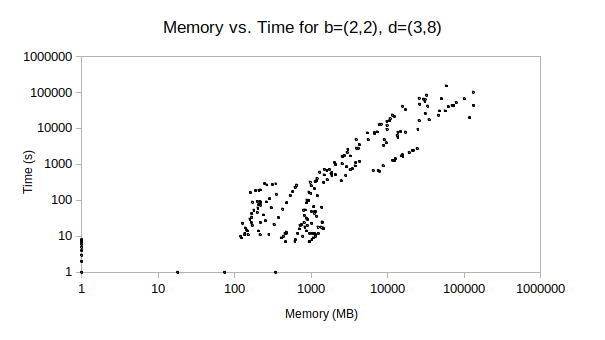
Figure 1. Memory vs. time to compute ranks of matrices for $\mathbf{b}=(2,2)$, $\mathbf{d}=(3,8)$

For concreteness, let us consider our largest complete computation, which is the case $\mathbf{b}=(2,2)$ and $\mathbf{d}=(3,8)$. The relevant range involves 1130 matrices, the largest of which is $2,124,896\times 3,719,448$, and Figure 1 provides a scatterplot of the time and memory involved in computing the ranks of those matrices. Only a handful of cases took over a day.

1.2. Computational improvements

Our current work improves on the method of [bruceErmanGoldsteinYang18] in a number of ways. Most notably, [bruceErmanGoldsteinYang18] relied on floating-point rank computations of sparse real matrices, using a MATLAB implementation of the LU-algorithm; by contrast, our current work simply performs the computations over finite fields in MAGMA. MAGMA recently introduced major improvements in their linear algebra of finite fields [steel], which seemed to make these rank computations much faster than our previous method; see Figure 2.

Method Average time per job (secs) Max time (secs)

MatLab LU-algorithm over $$\mathbb{R}$$ 220 4735

MAGMA rank algorithm over 7 99

Figure 2. We compared floating-point LU-algorithm computations in MatLab with rank computations in MAGMA over the finite field $\mathbb{F}_{32003}$, for all of the multigraded matrices related to one individual Betti number. This anecdotally suggests that MAGMA computations over finite fields are significantly faster, though we did not do any comprehensive testing.

Moreover, this switch to working over finite fields enabled us to use exact calculations, eliminating the need for floating-point approximations. While an exact computation over a finite field will not necessarily agree with the exact computation over $\mathbb{Q}$, there are only finitely many primes where the computations could disagree, and these discrepancies seem to rarely arise for reasonably large primes. This switch to working over finite fields thus had a significant downstream effect: the main computations in  [bruceErmanGoldsteinYang18] introduced some numerical errors as $\mathbf{d}$ grew larger, requiring the use of representation theoretic techniques to detect these errors. By contrast, our finite field computations produced no such numerical errors, and we were able to produce Schur functor decompositions without the need for the sort of “error correction” from [bruceErmanGoldsteinYang18, §5].

1.3. New Data

After computing the multigraded ranks for the relevant range, we process the data into usable formats. The rank computations quickly yield $\mathbb{Z}^{4}$-multigraded Betti numbers, but most mathematical conjectures focus on either the standard $\mathbb{Z}$-graded Betti numbers or on the underlying $\mathbf{GL}_{2}\times\mathbf{GL}_{2}$-Schur modules. We convert into those formats and encode all of the results into a Macaulay2 package for ease of use.

In total, we compute complete Betti tables for just shy of 200 total pairs of $\mathbf{b}$ and $\mathbf{d}$. See §3 and Table 1 for more details on the data.

1.4. Conjectures

Based on the data we computed, we develop a number of new conjectures, and we provided evidence in support of some previous conjectures.

We first examine the quantitative behavior of the standard grade Betti numbers, with conjectures in §LABEL:sec:qual_conjectures that address unimodality properties of the Betti numbers and various statistics. In addition, we consider our data in relation to a conjecture of Ein, Erman, and Lazarsfeld that, for large values of $\mathbf{d}$, the Betti numbers in any given row of the Betti table should behave like a binomial distribution [EEL, Conjecture B]. A theorem of Bruce [bruce-semiample, Theorem A] implies that the first row of the Betti table for $\mathbb{P}^{1}\times\mathbb{P}^{1}$ and line bundles $(2,d_{2})$ satisfies exactly this behavior as $d_{2}\to\infty$. Our data provides further support for the normal distribution behavior suggested by the conjecture, and seems to show this behavior even for the low values of $d_{2}$ for which we have data. See Figure 3.

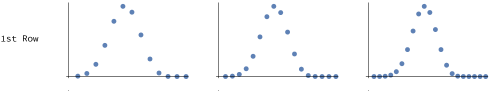
Figure 3. Here we plot the Betti numbers of the first row of the Betti tables of $\mathbb{P}^{1}\times\mathbb{P}^{1}$ embedded by $(d,3)$, for $d=3,4$ and $5$. They appear to resemble a normal distribution, as predicted by a conjecture of [EEL].

In §LABEL:sec:rep_theory_conjectures, we consider several conjectures related to the $\mathbf{GL}_{2}\times\mathbf{GL}_{2}$ structure of these syzygies. This includes precise conjectures on the Schur functor decomposition of certain entries; an analysis of the shapes of partitions that arise; and a discussion of “redundant” representations.

In §LABEL:sec:boij_sod, we present a collection of conjectures involving the Boij-Söderberg decompositions of these Betti tables. In particular, we provide a complete conjectural description of the Boij-Söderberg coefficients of the homogeneous coordinate ring of $\mathbb{P}^{1}\times\mathbb{P}^{1}$ embedded by $\mathcal{O}_{\mathbb{P}^{1}\times\mathbb{P}^{1}}(2,d_{2})$

2. Background and Notation

Throughout this section, we work over an arbitrary field $\mathbb{K}$. Our convention will be to write integer vectors using boldface, as in $\mathbf{d}\in\mathbb{Z}^{2}$, and to specify the coordinates as $\mathbf{d}=(d_{1},d_{2})$. We let $\mathbf{0}=(0,0)\in\mathbb{Z}^{2}$.

As we are interested in the syzygies of $\mathbb{P}^{1}\times\mathbb{P}^{1}$ throughout we let $S=\mathbb{K}[x_{0},x_{1},y_{0},y_{1}]$ be the corresponding polynomial of over a field $\mathbb{K}$. When viewed as the Cox ring of $\mathbb{P}^{1}\times\mathbb{P}^{1}$ [cox95], the ring $S$ inherits a $\mathbb{Z}^{2}$-bigrading given by $\deg x_{0}=\deg x_{1}=(1,0)\in\mathbb{Z}^{2}$ and $\deg y_{0}=\deg y_{1}=(0,1)\in\mathbb{Z}^{2}$. The ring $S$ also admits a $\mathbb{Z}^{4}$-multigrading given by setting the degree of each variable to be a generator of $\mathbb{Z}^{4}$, e.g. $\deg(x_{0})=(1,0,0,0)$ and $\deg(x_{1})=(0,1,0,0)$ and so on.

2.1. Standard graded Betti numbers

The syzygies of $\mathbb{P}^{1}\times\mathbb{P}^{1}$ under various embeddings come from studying Segre-Veronese modules of $S$. Given $\mathbf{d}\in\mathbb{Z}^{2}_{>0}$ and $\mathbf{b}\in\mathbb{Z}^{2}$ the Segre-Veronese module is

$$S(\mathbf{b};\mathbf{d})\coloneqq\bigoplus_{k\in\mathbb{Z}}S_{k\mathbf{d}+\mathbf{b}}.$$

Since $k\mathbf{d}+\mathbf{b}$ determines a ray in $\mathbb{Z}^{2}$ as $k$ varies in $\mathbb{Z}$, $S(\mathbf{b};\mathbf{d})$ is naturally a $\mathbb{Z}$-graded module over the polynomial $R=\operatorname{Sym}S_{\mathbf{d}}$. When $\mathbf{b}=\mathbf{0}$ the module $S(\mathbf{0};\mathbf{d})$ is isomorphic to the homogeneous coordinate ring of $\mathbb{P}^{1}\times\mathbb{P}^{1}$ embedded by $\mathcal{O}_{\mathbb{P}^{1}\times\mathbb{P}^{1}}(\mathbf{d})$ into the projective space $\mathbb{P}^{(\mathbf{d}_{1}+1)(\mathbf{d}_{2}+1)-1}=\operatorname{Proj}R$. If $\mathbf{b}\neq\mathbf{0}$, then $S(\mathbf{b};\mathbf{d})$ is naturally isomorphic to the section module of a pushforward of a line bundle; specifically, $S(\mathbf{b};\mathbf{d})$ is the $R$-module associated to the sheaf $(\iota_{\mathbf{d}})_{*}\mathcal{O}_{\mathbb{P}^{1}\times\mathbb{P}^{1}}(\mathbf{b})$. As noted in the introduction, while our primary interest is in the syzygies of the homogeneous coordinate rings $S(\mathbf{0};\mathbf{d})$, past work shows that studying the syzygies of other line bundles is often helpful in providing a more uniform picture [einLazarsfeld12, eel-quick, green-II].

The Betti numbers of a graded $R$-module $M$ are defined as $\beta_{i,j}(M)=\dim_{\mathbb{K}}\operatorname{Tor}^{R}_{i}(M,\mathbb{K})_{j}$, which denotes the degree $j$ part of the $\operatorname{Tor}_{i}$-module. For convenience, when studying the Betti numbers $S(\mathbf{b};\mathbf{d})$, we will omit reference to the ambient polynomial ring $R$, and write $\beta_{i,j}(S(\mathbf{b};\mathbf{d}))=\beta_{i,j}(\mathbb{P}^{1}\times\mathbb{P}^{1},\mathbf{b};\mathbf{d})$. The Betti numbers of a graded module are often computed using a minimal free resolution [eisenbud-syzygies, M2]. However, an alternate characterization of the Betti numbers, via Koszul cohomology, is more relevant for our computational approach.

The Koszul complex of $S(\mathbf{b};\mathbf{d})$ over the ring $R$ is the complex:

which is naturally $\mathbb{Z}$-graded since since $R$ is $\mathbb{Z}$-graded. Given a pair of integers $(p,q)$, we can analyze the cohomology of the degree $p+q$ strand of this complex, in homological degree $p$. This will be denoted by $K_{p,q}(\mathbb{P}^{1}\times\mathbb{P}^{1},\mathbf{b};\mathbf{d})$. It can be computed explicitly as the middle cohomology of the following complex:

(2.1)

where the differentials are given by

$$\partial_{p+1,q-1}\left(m_{0}\wedge m_{1}\wedge\cdots\wedge m_{p}\otimes f\right) =\sum_{i=0}^{p}(-1)^{i}m_{0}\wedge m_{1}\wedge\cdots\wedge\hat{m}_{i}\wedge\cdots\wedge m_{p}\otimes m_{i}f$$

$$\partial_{p,q}\left(m_{1}\wedge m_{2}\wedge\cdots\wedge m_{p}\otimes f\right) =\sum_{i=1}^{p}(-1)^{i}m_{1}\wedge m_{2}\wedge\cdots\wedge\hat{m}_{i}\wedge\cdots\wedge m_{p}\otimes m_{i}f.$$

In other words, instead of computing all of the Betti numbers simultaneously via a minimal free resolution, we can compute each Betti number individually using the complex of vector spaces in (2.1). This, in essence, turns a problem of symbolic algebra into a (massive but largely distributable) problem in linear algebra.

2.2. Multigraded Betti numbers

By incorporating the $\mathbb{Z}^{4}$-grading on $S$, we can subdivide the problem even further and obtain the $\mathbb{Z}^{4}$-graded Betti numbers. For a multidegree $\mathbf{e}\in\mathbb{Z}^{4}$, we define $\beta_{i,\mathbf{e}}(\mathbb{P}^{1}\times\mathbb{P}^{1},\mathbf{b};\mathbf{d})=\beta_{i,\mathbf{e}}(S(\mathbf{b};\mathbf{d}))=\dim_{\mathbb{K}}\operatorname{Tor}^{R}_{i}(S(\mathbf{b};\mathbf{d}),\mathbb{K})_{\mathbf{e}}$. This is well defined because both $R$ and $S(\mathbf{b};\mathbf{d})$ inherit $\mathbb{Z}^{4}$-multigradings from $S$. From the Koszul cohomology perspective, the Koszul complex of $S(\mathbf{b};\mathbf{d})$ over $R$ is also homogeneous with respect to the $\mathbb{Z}^{4}$-grading. Thus, we can analyze the cohomology of the degree $\mathbf{e}$-strand, which provides our method for computing $\beta_{i,\mathbf{e}}(\mathbb{P}^{1}\times\mathbb{P}^{1},\mathbf{b};\mathbf{d})$.

2.3. Schur functor decomposition

The action of $\mathbf{GL}_{2}\times\mathbf{GL}_{2}$ on $\mathbb{P}^{1}\times\mathbb{P}^{1}$ turns the vector space $K_{p,q}(\mathbb{P}^{1}\times\mathbb{P}^{1},\mathbf{b};\mathbf{d})$ into a $\mathbf{GL}_{2}\times\mathbf{GL}_{2}$-representation. We can therefore decompose $K_{p,q}(\mathbb{P}^{1}\times\mathbb{P}^{1},\mathbf{b};\mathbf{d})$ into a direct sum of irreducible $\mathbf{GL}_{2}\times\mathbf{GL}_{2}$-representations. These irreducible representations have the form $\mathbf{S}_{\lambda}\otimes\mathbf{S}_{\mu}$, where $\lambda,\mu$ are partitions with length $\leq 2$. See [FultonHarris, Exercise 2.36] for background. For brevity, we write $\mathbf{S}_{(a,b,c,d)}$ for the Schur module $\mathbf{S}_{(a,b)}\otimes\mathbf{S}_{(c,d)}$.

Example 2.2.

Let $\mathbf{b}=(2,2)$ and $\mathbf{d}=(3,3)$. The Betti table for $S(\mathbf{b};\mathbf{d})$ is

$$\begin{array}[]{ccccccccccccccc}&0&1&2&3&4&5&6&7&8&9&10&11&12&13\\ 0:&9&108&585&1872&3861&5148&4026&1080&\mathbf{165}&\cdot&\cdot&\cdot&\cdot&\cdot\\ 1:&\cdot&\cdot&\cdot&\cdot&\cdot&165&1080&4026&5148&3861&1872&585&108&9\end{array}$$

The bold entry in the Betti table tells us that $\dim K_{8,0}(\mathbb{P}^{1}\times\mathbb{P}^{1},\mathbf{b};\mathbf{d})=\beta_{8,8}(\mathbb{P}^{1}\times\mathbb{P}^{1},\mathbf{b};\mathbf{d})=165$. Viewed as $\mathbf{GL}_{2}\times\mathbf{GL}_{2}$-representation, $K_{8,0}(\mathbb{P}^{1}\times\mathbb{P}^{1},\mathbf{b};\mathbf{d})$ decomposes as

$$K_{8,0}(\mathbb{P}^{1}\times\mathbb{P}^{1},\mathbf{b};\mathbf{d})\cong\mathbf{S}_{(17,9,17,9)}\oplus\mathbf{S}_{(16,10,16,10)}\oplus\mathbf{S}_{(15,11,15,11)}\oplus\mathbf{S}_{(14,12,14,12)}\oplus\mathbf{S}_{(13,13,13,13)}.$$

The dimensions of these Schur modules are $81,49,25,9$ and $1$, respectively.

2.4. Koszul Duality

Using duality of Koszul cohomology groups (see, for instance [green-I, Duality Theorem (2.c.9)]), we can derive data for more values of $\mathbf{b}$ and $\mathbf{d}$, as we now explain. Given $\mathbf{b}$ we define its Koszul dual as $\mathbf{b}^{\prime}:=\mathbf{d}-\mathbf{b}-(2,2)$. We have

$$K_{p,q}(\mathbb{P}^{1}\times\mathbb{P}^{1},\mathbf{b}^{\prime};\mathbf{d})\cong K_{(d_{1}+1)(d_{2}+1)-3-p,2-q}(\mathbb{P}^{1}\times\mathbb{P}^{1},\mathbf{b};\mathbf{d})$$

as vector spaces. Visually, this means that the Betti table for $(\mathbf{b}^{\prime};\mathbf{d})$ is obtained by rotating the Betti table for $(\mathbf{b};\mathbf{d})$ by $180^{\circ}$. We will illustrate this phenomenon in Example 2.3. Note that $(d_{1}+1)(d_{2}+1)-3$ is the codimension of $\mathbb{P}^{1}\times\mathbb{P}^{1}$ in the embedding by $\mathbf{d}$. The duality also applies to the Schur functor decomposition via the following formula. To phrase this, we need some more notation. Let

$$\alpha:=\left(\tfrac{(d_{1}+1)(d_{2}+1)d_{1}-2}{2},\tfrac{(d_{1}+1)(d_{2}+1)d_{1}-2}{2},\tfrac{(d_{1}+1)(d_{2}+1)d_{2}-2}{2},\tfrac{(d_{1}+1)(d_{2}+1)d_{2}-2}{2}\right).$$

Given any $w=(w_{0},w_{1},w_{2},w_{3})\in\mathbb{Z}^{4}$ we write $w^{\text{opp}}=(w_{1},w_{0},w_{3},w_{2})$ and we choose $w^{\prime}$ so that $w+(w^{\prime})^{\text{opp}}=\alpha$. The multiplicity of the Schur functor $S_{w}$ in $K_{p,q}(\mathbf{b};\mathbf{d})$ equals the multiplicity of the Schur functor $S_{w^{\prime}}$ in the dual Koszul cohomology group $K_{(d_{1}+1)(d_{2}+1)-3-p,2-q}(\mathbb{P}^{1}\times\mathbb{P}^{1},\mathbf{b}^{\prime};\mathbf{d})$, where $\mathbf{b}^{\prime}$ is defined as above.

Example 2.3.

Let $\mathbf{b}=(0,0)$ and $\mathbf{d}=(3,3)$. The Betti table for $S(\mathbf{b};\mathbf{d})$ is

$$\begin{array}[]{ccccccccccccccc}&0&1&2&3&4&5&6&7&8&9&10&11&12&13\\ 0:&1&\cdot&\cdot&\cdot&\cdot&\cdot&\cdot&\cdot&\cdot&\cdot&\cdot&\cdot&\cdot&\cdot\\ 1:&\cdot&87&676&2691&6864&12155&15444&14157&9152&3861&780&\mathbf{22}&\cdot&\cdot\\ 2:&\cdot&\cdot&\cdot&\cdot&\cdot&\cdot&\cdot&\cdot&\cdot&\cdot&165&144&39&4\end{array}$$

The bold entry in the Betti table tells us that $\dim K_{11,1}(\mathbb{P}^{1}\times\mathbb{P}^{1},\mathbf{b};\mathbf{d})=\beta_{11,12}(\mathbb{P}^{1}\times\mathbb{P}^{1},\mathbf{b};\mathbf{d})=22$. Viewed as $\mathbf{GL}_{2}\times\mathbf{GL}_{2}$-representation, $K_{11,1}(\mathbb{P}^{1}\times\mathbb{P}^{1},\mathbf{b};\mathbf{d})$ decomposes as

$$K_{11,1}(\mathbb{P}^{1}\times\mathbb{P}^{1},\mathbf{b};\mathbf{d})\cong\mathbf{S}_{(23,13,18,18)}\oplus\mathbf{S}_{(18,18,23,13)}.$$

The Koszul dual pair to $(\mathbf{b};\mathbf{d})$ is $\mathbf{b}^{\prime}=(1,1)$ and $\mathbf{d}^{\prime}=(3,3)$. The Betti table for $S(\mathbf{b}^{\prime};\mathbf{d}^{\prime})$ is

$$\begin{array}[]{ccccccccccccccc}&0&1&2&3&4&5&6&7&8&9&10&11&12&13\\ 0:&4&39&144&165&\cdot&\cdot&\cdot&\cdot&\cdot&\cdot&\cdot&\cdot&\cdot&\cdot\\ 1:&\cdot&\cdot&\mathbf{22}&780&3861&9152&14157&15444&12155&6864&2691&676&87&\cdot\\ 2:&\cdot&\cdot&\cdot&\cdot&\cdot&\cdot&\cdot&\cdot&\cdot&\cdot&\cdot&\cdot&\cdot&1\end{array}$$

We see that this Betti table is exactly that corresponding to $S(\mathbf{b};\mathbf{d})$ rotated by $180^{\circ}$. The $(11,1)$ entry for $S(\mathbf{b};\mathbf{d})$ corresponds to $(2,1)$ for $S(\mathbf{b}^{\prime};\mathbf{d}^{\prime})$. Viewed as $\mathbf{GL}_{2}\times\mathbf{GL}_{2}$-representation, $K_{2,1}(\mathbb{P}^{1}\times\mathbb{P}^{1},\mathbf{b};\mathbf{d})$ decomposes as

$$K_{2,1}(\mathbb{P}^{1}\times\mathbb{P}^{1},\mathbf{b};\mathbf{d})\cong\mathbf{S}_{(10,0,5,5)}\oplus\mathbf{S}_{(5,5,10,0)}$$

3. Computed Data

Using the algorithms outlined in Section 4 we computed the Betti tables, $\mathbb{Z}^{4}$-multigraded Betti numbers, and Schur functor decompositions for over 150 distinct pairs $(\mathbf{b};\mathbf{d})$, including $27$ distinct $\mathbf{d}$-values. In Table 1, we list, for each $\mathbf{d}$, the number of $\mathbf{b}$’s for which we have complete data. For comparison:  [bruceErmanGoldsteinYang18] computed similar data for $\mathbb{P}^{2}$ for about $15$ distinct pairs $(\mathbf{b};\mathbf{d})$, which included $5$ distinct $\mathbf{b}$ values; and  [wcdl], which only considered the case $\mathbf{b}=\mathbf{0}$, computed data for $\mathbb{P}^{2}$ for $5$ distinct $\mathbf{d}$ values. There appears to be no significant computational work on syzygies for $\mathbb{P}^{1}\times\mathbb{P}^{1}$, although [lemmensP1P1] does construct a non-minimal resolution. In other words, these computations represent a significant contribution to the available syzygy data for $\mathbb{P}^{1}\times\mathbb{P}^{1}$ specifically, as well as for toric surfaces more generally.

						$d_{2}$
		2	3	4	5	6	7	8	9	10
	2	3	6	8	10	12	14	13	6	6
$d_{1}$	3	$\cdot$	6	12	15	13	12	8	4	2
	4	$\cdot$	$\cdot$	9	14	9	5	1	1	0
	5	$\cdot$	$\cdot$	$\cdot$	1	1	1	1	0	0

Table 1. For each $\mathbf{d}$, the number of $\mathbf{b}$ for which we compute the Betti tables, $\mathbb{Z}^{4}$-multigraded Betti numbers, and Schur decompositions

Remark 3.1.

In Table 1, for the symmetric cases $\mathbf{d}=(d,d)$, we only record $\mathbf{b}=(b_{1},b_{2})$ with $b_{1}\leq b_{2}$ for which we have data. For example, when $\mathbf{d}=(2,2)$, we only count the cases $\mathbf{b}=(0,0)$, $(0,1)$, and $(1,1)$; we do not include $(1,0)$.

4. Main Computation

Broadly speaking, our approach to computing the Betti table, $\mathbb{Z}^{4}$-multigraded Betti numbers, and Schur functor decompositions for a given pair $(\mathbf{b};\mathbf{d})$ proceeds as follows:

1. Reduction to the relevant range: By combining a computation of the multigraded Hilbert series with known vanishing results for syzygies (relying primarily on Castelnuovo-Mumford regularity), we conclude that a small subset of the Betti numbers determines all of the Betti numbers. This smaller subset is the relevant range, and is the focus of our computations.

2. Constructing the matrices in the relevant range: We follow the ideas in [bruceErmanGoldsteinYang18] to efficiently construct and store the matrices from the relevant range.

3. High throughput rank computations: We use distributed high throughput computation to find the ranks of all the matrices in the relevant range. These computations are done via linear algebra over the finite field $\mathbb{F}_{32003}$ in MAGMA. This is by far the most computationally intensive aspect.

4. Post-processing: Using standard ideas from representation theory, we convert the multigraded Betti number into Schur functor decompositions.

While the techniques here are broadly similar to those in [bruceErmanGoldsteinYang18], which focused on computing syzygies of Veronese embeddings of $\mathbb{P}^{2}$, the passage from $\mathbb{P}^{2}$ to $\mathbb{P}^{1}\times\mathbb{P}^{1}$ requires new code in each step and we further refine this implementation and approach. The most significant distinction is in the third step abvoe: the core algorithm in the current work uses linear algebra over finite fields, whereas in  [bruceErmanGoldsteinYang18] it used floating-point computations.

4.1. Relevant Range

We expedite our computations significantly by utilizing the fact that for many values of $p$ and many multidegrees $\mathbf{a}$, the multigraded Betti number $\beta_{p,\mathbf{a}}(\mathbb{P}^{1}\times\mathbb{P}^{1},\mathbf{b};\mathbf{d})$ is determined entirely by the $\mathbb{Z}^{4}$-multigraded Hilbert series of $S(\mathbf{b};\mathbf{d})$. In the following lemma, we use vector notation $t^{\mathbf{a}}:=t_{0}^{a_{0}}t_{1}^{a_{1}}t_{2}^{a_{2}}t_{3}^{a_{3}}$ if $\mathbf{a}=(a_{0},a_{1},a_{2},a_{3})$.

Lemma 4.1.

The $\mathbb{Z}^{4}$-multigraded Hilbert series of $S(\mathbf{b};\mathbf{d})$ is a rational function of the form: $A(t_{0},t_{1},t_{2},t_{3})/B(t_{0},t_{1},t_{2},t_{3})$ where

$$A=\sum_{p,\mathbf{a}}\beta_{p,\mathbf{a}}(\mathbb{P}^{1}\times\mathbb{P}^{1},\mathbf{b};\mathbf{d})t^{\mathbf{a}}\text{ and }B=\prod_{\mathbf{b}\in\mathbb{N}^{4},b_{0}+b_{1}=d_{1},b_{2}+b_{3}=d_{2}}(1-t^{\mathbf{b}})$$

The proof is nearly identical to that of [bruceErmanGoldsteinYang18, Lemma 3.1], so we omit it.

With this in mind, our main computations reduce to determining the ranks $\partial_{p,q}$ for $p,q$ in what we call the relevant range.

Definition 4.2.

Fixing $\mathbf{b}$ and $\mathbf{d}$ we define the relevant range to be the set of pairs $(p,q)$ such that $K_{p,q}(\mathbb{P}^{1}\times\mathbb{P}^{1},\mathbf{b};\mathbf{d})\neq 0$ and either $K_{p-1,q+1}(\mathbb{P}^{1}\times\mathbb{P}^{1},\mathbf{b};\mathbf{d})\neq 0$ or $K_{p+1,q-1}(\mathbb{P}^{1}\times\mathbb{P}^{1},\mathbf{b};\mathbf{d})\neq 0$.

In general we determine the relevant range by finding the smallest $p$ such that $K_{p,q}(\mathbb{P}^{1}\times\mathbb{P}^{1},\mathbf{b};\mathbf{d})\neq 0$ and then applying duality (see [einLazarsfeld12, Proposition 3.5]). When $\mathbf{b}=\mathbf{0}$ the only case of interest is $q=1$, and we find the smallest $p$ such that $K_{p,1}(\mathbb{P}^{1}\times\mathbb{P}^{1},\mathbf{0};\mathbf{d})\neq 0$ via [wcdl, Theorem 1.4]. When $\mathbf{b}\neq\mathbf{0}$ we determine the relevant range using the fairly coarse vanishing bounds from [einLazarsfeld12, Proposition 5.1]. While a sharper bound on the relevant range would allow us to compute ranks for many fewer matrices, we found that in practice, these potentially extraneous matrices did not cause any bottlenecks in the actual computation.

An algorithm entirely analogous to [bruceErmanGoldsteinYang18, Algorithm 3.3] enables us to efficiently compute the multigraded Betti numbers outside of the relevant range.

4.2. Constructing the matrices in the relevant range

After computing the relevant range and the relevant multidegrees, this data is fed to the code to compute the matrices representing the differentials in the relevant range. We first use the $\mathfrak{S}_{2}\times\mathfrak{S}_{2}$-symmetries of the multidegrees to restrict to those multidegrees $(a,b,c,d)$ where $a\geq b$ and $c\geq d$. As in [bruceErmanGoldsteinYang18] we use duality for Koszul cohomology groups to reduce the number of matrices we compute [green-I, Theorem 2.c.6]. Unfortunately unlike in the case of the Veronese, the bi-graded structure means that it is not possible to use this duality to reduce to a finite set of non-redundant Betti tables.

When constructing the matrices, we use the fact that all of the maps $(\partial_{p,q})_{\mathbf{a}}$ correspond to submatrices of the boundary map $d_{p}:\bigwedge^{p}S_{\mathbf{d}}\rightarrow\bigwedge^{p-1}S_{\mathbf{d}}$. In particular, $(\partial_{p,q})_{\mathbf{a}}$ is given by restricting to the submatrix $d_{p,\leq\mathbf{a}}$ given by those entries in degrees $\leq\mathbf{a}$. However, instead of storing the map $d_{p}$ we simply use this fact to compute all of the various $(\partial_{p,q})_{\mathbf{a}}$ for all multidegrees at once. This was implemented as it was found that as the degrees got larger, more of the entries in the $d_{p}$ matrix correspond to multidegrees that are not in the relevant range. This is entirely analogous to [bruceErmanGoldsteinYang18, §4.1], which provides further details. In Appendix LABEL:appendix:matrices, we list the number of matrices we must compute and the largest such matrix.

Example 4.3.

For $\mathbf{d}=(3,8)$, $\mathbf{b}=(2,2)$, the full computation of which is discussed in more detail in Example 4.4, it took a modern laptop computer, 5min 25sec to compute all the relevant matrices, entailing a total of 1130 matrices, taking a total of 13GB of space. The single largest matrix had 16,999,168 non-zero entries.

4.3. High Throughput Computations

The rank computations can be efficiently distributed over numerous different computers. We implemented these computations using high throughput computing via HTCondor on the University of Wisconsin–Madison Mathematics department computer servers. Many of the matrices are small, and hence do not require much memory to compute the rank. Because our hardware grid has fewer nodes with large amounts of available RAM, the initial submissions are allocated a small amount of RAM (e.g. 2GB). For the jobs that fail, we resubmit with a larger memory allocation, and repeat this process until the computation terminates.

Example 4.4.

In this example, we provide a detailed analysis of how we determine the Betti table for $\mathbf{d}=(3,8)$ and $\mathbf{b}=(2,2)$, one of our larger computations. There are only two rows $q=0,1$, and 34 columns; we display the first several columns below.

$$\begin{array}[]{ccccccccccc}&0&1&2&3&4&5&6&7&8&9\\ 0:&9&258&3465&28512&156546&568620&1210506&697680&203490&\cdot\\ 1:&\cdot&\cdot&\cdot&1050&28476&498498&5444400&41855958&194378184&671067540\\ \end{array}\cdots$$

The relevant range is $(p,0)$ for $4\leq p\leq 8$ and $(p,1)$ for $3\leq p\leq 7$. Because $K_{p,0}-K_{p-1,1}$ is determined by the Hilbert function of the module, we need only compute one of $K_{p,0}$ or $K_{p-1,1}$, and we compute the former. To that end, we form the matrices $(\partial_{p,0})_{\mathbf{a}}$ and $(\partial_{p+1,-1})_{\mathbf{a}}$ for $4\leq p\leq 8$ and compute their ranks. Fortunately, $(\partial_{p+1,-1})_{\mathbf{a}}=0$. After accounting for $\mathfrak{S}_{2}\times\mathfrak{S}_{2}$-symmetry, we are left to compute ranks of $1130$ matrices, the largest of which is $2,\!124,\!896\times 3,\!719,\!448$. In this case, up to symmetry there were 39788 multidegrees with non-zero entries in the Betti table. For these entries, in absence of the consideration about relevant ranges, to compute these entries would have required the computation of at least $81,\!437$ matrices.

The amount of RAM and time used in the rank calculation is recorded in Figure 1. The vast majority of matrices require less than 1MB of RAM and 10 seconds. Figure 4 has two plots displaying the average and maximum memory, resp. time, needed to compute the ranks of the matrices $(\partial_{p,0})_{\mathbf{a}}$ as a function of $p$.

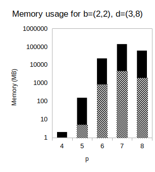
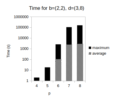
Figure 4. Memory and time to compute ranks of matrices for $\mathbf{b}=(2,2)$, $\mathbf{d}=(3,8)$ and $q=0$

Figure LABEL:fig:heatMapMultidegree illustrates how memory usage varies with multidegree for each $(p,0)$. The plots are arranged left to right $(p,q)=(4,0)$ through $(8,0)$. Here is how to interpret these plots. Within each plot, each square represents a multidegree, and its color measures the memory usage: light gray is 0 GB and black reaches the maximum of 132 GB of RAM. Because of the $\mathfrak{S}_{2}\times\mathfrak{S}_{2}$-symmetry, we need only consider the multidegrees $(a,b,c,d)$ satisfying $a+b=26$, $a\leq b$ and $c+d=66$, $c\leq d$. Each row has $(a,b)$ constant, each column has $(c,d)$ constant, and $a$, resp. $c$, increases in the downward, resp. left, direction.