Direct photons emission rate and electric conductivity in twice anisotropic QGP holographic model with first-order phase transition

Abstract

The electric conductivity and direct photons emission rate are considered in the holographic theory with two types of anisotropy. The electric conductivity is derived in two different ways, and their equivalence for the twice anisotropic theory is shown. Numerical calculations of the electric conductivity were done for Einstein-dilaton-three-Maxwell holographic model [29]. The dependence of the conductivity on the temperature, the chemical potential, the external magnetic field, and the spatial anisotropy of the heavy-ions collision (HIC) is studied. The electric conductivity jumps near the first-order phase transition are observed. This effect is similar to the jumps of holographic entanglement that were studied previously.

1 Introduction

The thermal-photon production in heavy-ion collisions plays an essential role in studying the quark-gluon plasma (QGP). Photons can be considered as probes of QGP because they do not interact with hadronic plasma. Experimental study of the production of thermal photons provides knowledge about many characteristics of QGP [1]. In particular, the rate of photon production is related to the electric conductivity of QGP [2].

To compare HIC experimental data to theoretical calculations, one needs non-perturbative calculations in QCD. A holographic approach is an effective tool for non-perturbative studies of QGP [3, 4, 5]. The present investigation is significant in the scope of recent experiments in high energy physics: FAIR and NICA projects.

There is rich literature devoted to holographic calculations of electric conductivity [7, 2, 6, 8, 9, 10, 11, 12]. The holographic calculations of electric conductivity are related to the retarded correlator of currents in momentum space [2, 16, 13, 14, 15]. There are two different ways to find electric conductivity. In the first scheme [13, 14, 15, 10], one calculates the retarded Green function using equations of motion. In the alternative approach, one uses the membrane paradigm [17]. All previous calculations consider isotropic [10] or only partially anisotropic holographic models [6, 7, 11, 12], in the later case only part of coordinates enter the metric with different scale functions.

The choice of different warp factors distinguishes isotropic and anisotropic holographic QCD models [3, 4, 5, 18, 19, 20, 21, 22, 23, 25, 24, 26, 30, 31, 29, 27, 28, 33, 32, 34, 35, 38, 37, 36]. Many models establish the essential influence of anisotropy on the properties of QGP observables [39, 44, 40, 41, 42, 43]. Note that there are many studies on electric conductivity in inhomogeneous condensed matter systems [45, 46, 47]. Also, account for non-zero chemical potential dramatically changes the phase structure of QCD [11, 19, 21, 22, 23, 24, 28, 29, 30, 31, 34, 38, 27, 26, 32, 37]. Previous studies have revealed close relation of anisotropic models with magnetic field and influence of magnetic field on observables in QGP are considered in [7, 9, 26, 25, 34, 33] and [29, 31, 27, 12, 35].

This paper studies direct photons moving through twice anisotropic QGP and investigates influence of chemical potential and magnetic field on the results. So, we aim at calculating the Green function and determining the electric conductivity tensor in twice anisotropic holographic theory. Following the two aforementioned prescriptions, we calculate the retarded Green’s functions and demonstrate the agreement of these two approaches. We chose the five-dimensional twice anisotropic holographic model for heavy quarks based on Einstein-dilaton-three-Maxwell action [29] for our calculations. The warp-factor in this model is chosen to reproduce the phase transitions structure for heavy quarks of the Columbia plot [48, 49]. The first Maxwell field in action is related to chemical potential; the second describes spatial anisotropy, and the third accounts for an external magnetic field. In this model, a significant influence of the external magnetic field on the black hole solution and the confinement/deconfinement phase diagram was studied in [29]. In this model, we consider the impact of anisotropy, chemical potential and magnetic fields on electric conductivity.

We compare our results with lattice calculations. The electric conductivity was studied in isotropic lattice and in the vicinity of zero chemical potential [50, 51, 52, 53]. Therefore, we compare our results with lattice calculations only for the isotropic ($\nu=1$) case with zero chemical potential ($\mu=0$). We reproduce the lattice data by varying the kinetic potential for the Maxwell field (see Fig.3 below). With this universal kinetic function we calculate the DC conductivity for all other cases, i.e. anisotropic collisions ($\nu>1$), non-zero chemical potential ($\mu>0$) and non-zero magnetic field.

The paper is organized as follows. In Sect.2, the holographic model and perturbation action are described. In Sect.3, formulas for conductivity are obtained in twice anisotropic theory. In Sect.4 numerical results are presented. In Sect.5 we summarize the obtained results and link them to such quantities as the butterfly velocity, drag forces and the tension of the Wilson loop. Appendix A shows the alternative calculations of QGP DC conductivity. The cumulative tables Table 1 and Table 2 in Appendix B present plots for different set of parameters.

2 Setup

2.1 Holographic model

It was recognized that [54, 55, 56, 57, 44, 58] it is important to add anisotropy in the holographic theory as QGP is an anisotropic media just after the HIC, and an estimation for isotropisation time is about $1$–$5$ fm/c $\sim 10^{-24}$ s [59]. One of motivations to deal with anisotropic models is related with the problem of getting experimental data for the energy dependence of the total multiplicity of particles created in heavy-ion collisions [60]. Isotropic holographic models had not been able to reproduce the experimental multiplicity dependence on energy ([44] and refs therein), and to reproduce them anisotropic models of Lifshitz type with a parameter $\nu$ were considered. It’s value of about $\nu=4.5$ gives the dependence of the produced entropy on energy in accordance with the experimental data for the energy dependence of the total multiplicity of particles created in heavy-ion collisions (results by ATLAS and ALICE) [61, 60]. Anisotropy is also related with strong magnetic fields typical for HIC [62, 63, 64, 65, 66].

We consider an anisotropic holographic model [29] based on the action:

$$S_{bck}=\cfrac{1}{16\pi G_{5}}\int d^{5}x\ \sqrt{-g} \cdot \Big{[}R-\cfrac{f^{(1)}(\phi)}{4}\ F^{(1)^{2}}-\cfrac{f^{(2)}(\phi)}{4}\ F^{(2)}\,{}^{2}$$

$$-\cfrac{f^{(B)}(\phi)}{4}\ F^{(B)}\,{}^{2}-\cfrac{1}{2}\ \partial_{\mu}\phi\partial^{\mu}\phi-V(\phi)\Big{]}.$$

This action contains three different Maxwell fields with their own dilaton-dependent coupling functions and each of these fields has its own interpretation. With help of $F^{(1)}$ and $F^{(2)}$ the chemical potential and anisotropy are introduced, and $F^{(B)}$ describes the external magnetic field.

The ansatz for the metric is

$$ds^{2}=\frac{L^{2}\mathfrak{b}(z)}{z^{2}}\left[-g(z)dt^{2}+\mathfrak{g}_{1}(z)dx_{1}^{2}+\mathfrak{g}_{2}(z)dx_{2}^{2}+\mathfrak{g}_{3}(z)dx_{3}^{2}+\frac{dz^{2}}{g(z)}\right],\\$$ (2.2)

where $L$ is the AdS-radius, $\mathfrak{b}(z)$ is the warp-factor, $g(z)$ is the blackening function, and we will consider $\mathfrak{g}_{i}$ of the special forms

$$\mathfrak{g}_{1}=1,\quad\mathfrak{g}_{2}(z)=\left(\frac{z}{L}\right)^{2-\frac{2}{\nu}},\quad\mathfrak{g}_{3}(z)=e^{c_{B}z^{2}}\left(\frac{z}{L}\right)^{2-\frac{2}{\nu}}.$$ (2.3)

The special form of prefactors $\left(\frac{z}{L}\right)^{2-\frac{2}{\nu}}$ describes non-symmetry of heavy-ion collision (HIC), and $c_{B}$ is the coefficient of secondary anisotropy related to the external magnetic field. The specific choice of the warp-factor $\mathfrak{b}(z)$ determines the phase transitions structure of the model. The warp-factor of the form $\mathfrak{b}(z)=e^{-cz^{2}/2}$ reproduces the heavy quarks’ phase transitions structure of the Columbia plot [48, 49, 50, 51]. The warp-factor $\mathfrak{b}(z)=e^{-2a\ln(bz^{2}+1)}$ describes the light quarks’ case. The explicit solutions for the blackening function $g$, the gauge kinetic functions $f_{0}$, $f_{2}$ and $f_{B}$, the dilaton field, and the dilaton field potential $V$ are given in [29].

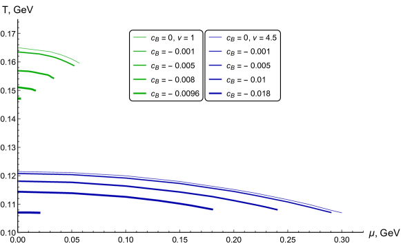
Figure 1: The BB phase transitions structure from [29] for different anisotropy parameter $\nu$ and magnetic field’s parameter $c_{B}$.

This model’s phase transition structure is presented in Fig.1. A remarkable feature of Einstein-dilaton-Maxwell models is the Van der Waals type of the temperature dependence on the size of horizon $z_{h}$. The temperature function can be three-valued for some values of parameters (chemical potential, anisotropy, magnetic field etc.). The Hawking-Page phase transition between AdS Black Hole and thermal AdS occurs in these models for zero chemical potential. For any non-zero chemical potential, there is a phase transition between small and large black holes. Even for zero chemical potential but non-zero magnetic field, the phase transition becomes the phase transition between small and large black holes (BB). For these phase transitions, such values as entropy, holographic entanglement entropy, and baryon density can experience a jump [68, 28]. In this work we observe the jump of electric conductivity at the temperature of BB phase transition, see next Sect.4.

To investigate properties of direct photons in heavy-ion collisions using holographic duality one has to introduce one more Maxwell field [7, 2, 6, 8, 9, 69, 10, 11, 12, 16, 17]. It is described by an action

$$S_{out}=-\frac{1}{4}\int d^{5}x\sqrt{-g}f_{0}F_{MN}F^{MN},$$ (2.4)

here $f_{0}=f_{0}(\phi)$ is the function of coupling of the Maxwell field to the dilaton (also called the gauge kinetic function) and we use capital Latin letters to number components of 5-dim objects $M=0,1,2,3,4$ and Greek letters for objects on 4-dim Minkowski spacetime $\mu=0,1,2,3$. The choice of $f_{0}$ function allows one to fit lattice results, see below Sect.4.2. Proceeding with a variational procedure for $S_{out}$, one finds

$$\delta S_{out}=-\int_{\partial\Omega}d\omega\sqrt{-g}f_{0}n_{M}F^{MN}\delta A_{N}+\int_{\Omega}d^{5}x\partial_{M}(\sqrt{-g}f_{0}F^{MN})\delta A_{N}=0,$$ (2.5)

where the manifold $\partial\Omega$ we integrate over is the 4-dim Minkowski space-time, $d\omega=d^{4}x$ is measure on the aforementioned manifold and $n_{M}$ is the outward unit normal vector to the boundary: $n_{M}=(0,0,0,0,1)$ on the horizon $z=z_{h}$ and $n_{M}=(0,0,0,0,-1)$ on the boundary $z=0$. Therefore, to get rid of surface terms one adds to $S_{out}$ the surface term $S_{sur\!f}$ and considers it as an addition to the initial action of the theory. The surface term in this case is

$$S_{sur\!f}=\left.\int d^{4}x\sqrt{-g}f_{0}F^{4\mu}A_{\mu}\right|^{z=z_{h}}_{z=0}.$$ (2.6)

This form of $S_{sur\!f}$ is essential in the so-called ’membrane paradigm’ [17, 16]. Then equations of motion are just Maxwell’s equations

$$\partial_{M}(\sqrt{-g}f_{0}F^{MN})=0.$$ (2.7)

2.2 Direct photons emission rate and electric conductivity

The number of photons emitted per unit time per unit volume $\Gamma$ (photon emission rate) in thermal equilibrium is given by the light-like correlator [70, 69]

$$d\Gamma=-\frac{d\mathbf{k}}{(2\pi)^{3}}\frac{e^{2}n_{b}(|\mathbf{k}|)}{|\mathbf{k}|}\operatorname{Im}\left[\eta_{\mu\nu}G^{\mu\nu}_{R}\right]_{k^{0}=|\mathbf{k}|},$$ (2.8)

where

$$n_{b}(|\mathbf{k}|)=\frac{\mathcal{A}}{\mathrm{e}^{-|\mathbf{k}|/T}-1}$$

is Bose-Einstein thermal distribution function, $\eta_{\mu\nu}$ is Minkowski metric tensor, photon’s 4-momentum is $k^{\mu}=(k^{0},\mathbf{k})$. Note that the retarded Green’s function $G_{R}^{\mu\nu}$ is related to the electric conductivity through the Kubo relation

$$\sigma^{\mu\nu}=-\frac{G_{R}^{\mu\nu}}{iw},$$

so the direct photons emission rate is connected to the conductivity of QGP.

3 Electric conductivity in twice anisotropic background

To find the electric conductivity, we add a probe Maxwell field (2.4) to (2.1). Consider an ansatz for this probe field in the form of a plane wave propagating in $x_{3}$ direction

$$A_{M}({t},{x_{3}},{z}){=}\psi_{M}(z)\exp(-i(wt-k{x_{3}})),\qquad M=0,...4.$$ (3.1)

From the equation of motion for $A_{4}(t,x_{3},z)$ (from this moment we write $A_{M}=A_{M}({t},{x_{3}},{z})$ for shorthand) component it follows that

$$\psi_{4}(z)\text{=}i\frac{-kg(z)\psi_{3}^{\prime}(z)-w\mathfrak{g}_{3}(z)\psi_{0}^{\prime}(z)}{k^{2}g(z)-w^{2}\mathfrak{g}_{3}(z)},$$ (3.2)

where ^′ denotes derivative with respect to $z$.

We also introduce notation for the longitudinal component of electric field

$$E_{3}=F_{03}=wA_{3}+kA_{0}$$ (3.3)

and for two transverse components as

$$E_{i}=wA_{i},\qquad i=1,2.$$ (3.4)

For brevity we drop out arguments of the blackening function $g$, anisotropy functions $\mathfrak{g}_{1},\,\mathfrak{g}_{2},\,\mathfrak{g}_{3}$, the gauge kinetic function $f_{0}$ and the warp-factor $\mathfrak{b}$ in the following equations. Thus equations of motions are

$$E_{3}^{\prime\prime}+E_{3}^{\prime}\left(\dfrac{\mathfrak{b}^{\prime}}{2\mathfrak{b}}+\dfrac{f_{0}^{\prime}}{f_{0}}-\dfrac{w^{2}\mathfrak{g}_{3}g^{\prime}}{k^{2}g^{2}-w^{2}g\mathfrak{g}_{3}}+\dfrac{w^{2}\mathfrak{g}_{3}^{\prime}}{k^{2}g-w^{2}\mathfrak{g}_{3}}+\dfrac{\mathfrak{g}_{1}^{\prime}}{2\mathfrak{g}_{1}}+\dfrac{\mathfrak{g}_{2}^{\prime}}{2\mathfrak{g}_{2}}+\dfrac{\mathfrak{g}_{3}^{\prime}}{2\mathfrak{g}_{3}}-\dfrac{1}{z}\right)+$$

$$+E_{3}\dfrac{w^{2}\mathfrak{g}_{3}-k^{2}g}{g^{2}\mathfrak{g}_{3}}=0;$$ (3.5)

$$E_{1}^{\prime\prime}+E_{1}^{\prime}\left(\dfrac{\mathfrak{b}^{\prime}}{2\mathfrak{b}}+\dfrac{f_{0}^{\prime}}{f_{0}}+\dfrac{g^{\prime}}{g}+\dfrac{\mathfrak{g}_{2}^{\prime}}{2\mathfrak{g}_{2}}+\dfrac{\mathfrak{g}_{3}^{\prime}}{2\mathfrak{g}_{3}}-\dfrac{\mathfrak{g}_{1}^{\prime}}{2\mathfrak{g}_{1}}-\dfrac{1}{z}\right)+E_{1}\dfrac{w^{2}\mathfrak{g}_{3}-k^{2}g}{g^{2}\mathfrak{g}_{3}}=0;$$ (3.6)

$$E_{2}^{\prime\prime}+E_{2}^{\prime}\left(\dfrac{\mathfrak{b}^{\prime}}{2\mathfrak{b}}+\dfrac{f_{0}^{\prime}}{f_{0}}+\dfrac{g^{\prime}}{g}+\dfrac{\mathfrak{g}_{1}^{\prime}}{2\mathfrak{g}_{1}}+\dfrac{\mathfrak{g}_{3}^{\prime}}{2\mathfrak{g}_{3}}-\dfrac{\mathfrak{g}_{2}^{\prime}}{2\mathfrak{g}_{2}}-\dfrac{1}{z}\right)+E_{2}\dfrac{w^{2}\mathfrak{g}_{3}-k^{2}g}{g^{2}\mathfrak{g}_{3}}=0.$$ (3.7)

Then the on-shell action is

$$S_{sur\!f}=\int\frac{d^{4}k}{(2\pi)^{4}}\frac{f_{0}\,g}{z}\left(\left.\mathcal{E}^{*}_{1}\sqrt{\frac{\mathfrak{b}\,\mathfrak{g}_{3}\mathfrak{g}_{2}}{\mathfrak{g}_{1}}}\mathcal{E}^{\prime}_{1}+\mathcal{E}^{*}_{2}\sqrt{\frac{\mathfrak{b}\,\mathfrak{g}_{3}\mathfrak{g}_{1}}{\mathfrak{g}_{2}}}\mathcal{E}^{\prime}_{2}-\mathcal{E}_{3}^{*}\frac{\sqrt{\mathfrak{b}\,\mathfrak{g}_{1}\mathfrak{g}_{2}\mathfrak{g}_{3}}}{\frac{k^{2}}{w^{2}}g-\mathfrak{g}_{3}}\mathcal{E}^{\prime}_{3}\right)\right|_{z=0}^{z=z_{h}},$$ (3.8)

where $\mathcal{E}_{i}={E_{i}}/{w}$ for $i=1,2,3$.

Following [16, 10] we make the on-shell action quadratic by introducing a new variable $\zeta_{3}$ proportional to canonical momentum of field $\mathcal{E}_{3}$

$$\zeta_{3}=-\frac{\mathcal{E}^{\prime}_{3}}{\mathcal{E}_{3}}\frac{2f_{0}g}{z}\frac{\sqrt{\mathfrak{b}\,\mathfrak{g}_{1}\mathfrak{g}_{2}\mathfrak{g}_{3}}}{\mathfrak{g}_{3}-g\frac{k^{2}}{w^{2}}}.$$ (3.9)

For further convenience we define

$$B_{3}\equiv\frac{2f_{0}g}{z}\frac{\sqrt{\mathfrak{b}\,\mathfrak{g}_{1}\mathfrak{g}_{2}\mathfrak{g}_{3}}}{\mathfrak{g}_{3}-g\frac{k^{2}}{w^{2}}}.$$ (3.10)

For the longitudinal direction the equation of motion (3) becomes

$$\frac{\mathcal{E}_{3}^{\prime\prime}}{\mathcal{E}_{3}}=\zeta_{3}\frac{B_{3}^{\prime}}{B_{3}^{2}}-\frac{w^{2}\mathfrak{g}_{3}-k^{2}g}{g^{2}\mathfrak{g}_{3}}.$$ (3.11)

Taking derivative of $\zeta_{3}$ with respect to $z$

$$\zeta_{3}^{\prime}=-\frac{\mathcal{E}_{3}^{\prime\prime}}{\mathcal{E}_{3}}B_{3}+\frac{B_{3}^{\prime}}{B_{3}}\zeta_{3}+\frac{\zeta_{3}^{2}}{B_{3}}=-\frac{\zeta_{3}B_{3}^{\prime}}{B_{3}}+B_{3}\frac{w^{2}\mathfrak{g}_{3}-k^{2}g}{g^{2}\mathfrak{g}_{3}}+\frac{\zeta_{3}B_{3}^{\prime}}{B_{3}}+\frac{\zeta_{3}^{2}}{B_{3}}.$$ (3.12)

Finally, the differential equation on $\zeta_{3}$ is

$$\left(\frac{\zeta_{3}}{w}\right)^{\prime}-\frac{f_{0}\sqrt{\mathfrak{b}\,\mathfrak{g}_{1}\mathfrak{g}_{2}\mathfrak{g}_{3}}}{\mathfrak{g}_{3}-g\frac{k^{2}}{w^{2}}}\frac{w}{zg}\left[\left(\frac{\zeta_{3}}{w}\right)^{2}\left(\frac{\mathfrak{g}_{3}-g\frac{k^{2}}{w^{2}}}{2f_{0}\sqrt{\mathfrak{b}\,\mathfrak{g}_{1}\mathfrak{g}_{2}\mathfrak{g}_{3}}}z\right)^{2}+\frac{\mathfrak{g}_{3}-g\frac{k^{2}}{w^{2}}}{\mathfrak{g}_{3}}\right]=0$$ (3.13)

We require $\zeta_{3}^{\prime}(z)\neq\infty$ for all $z$ since this quantity is related to observable values. The blackening function vanishes on the horizon, making the second term infinite. We are performing series expansion for both the blackening function (A.9) and the function inside square brackets (denote it $U(z)$ for convenience) near the horizon

$$U(z) = \left(\dfrac{\zeta_{3}}{w}\right)^{2}\left(\dfrac{\mathfrak{g}_{3}-g\frac{k^{2}}{w^{2}}}{2f_{0}\sqrt{\mathfrak{b}\,\mathfrak{g}_{1}\mathfrak{g}_{2}\mathfrak{g}_{3}}}z\right)^{2}+\dfrac{\mathfrak{g}_{3}-g\frac{k^{2}}{w^{2}}}{\mathfrak{g}_{3}}=$$ (3.14)

$$= U(z_{h})+U^{\prime}(z_{h})(z-z_{h})+o(z-z_{h})^{2}.$$

Clearly, the pole at $z=z_{h}$ cancels if $U(z_{h})=0$. This requirement translates into boundary condition for the Cauchy problem (3.13)

$$\zeta_{3}(z_{h})=2iw\frac{f_{0}(z_{h})}{z_{h}}\sqrt{\frac{\mathfrak{b}(z_{h})\mathfrak{g}_{1}(z_{h})\mathfrak{g}_{2}(z_{h})}{\mathfrak{g}_{3}(z_{h})}}.$$ (3.15)

In the low-frequency limit $w\rightarrow 0$, the equation (3.13) simply becomes

$$\zeta_{3}^{\prime}(z)=0.$$ (3.16)

Therefore, the solution for all values of $z$ is

$$\zeta_{3}=2iw\frac{f_{0}(z_{h})}{z_{h}}\sqrt{\frac{\mathfrak{b}(z_{h})\mathfrak{g}_{1}(z_{h})\mathfrak{g}_{2}(z_{h})}{\mathfrak{g}_{3}(z_{h})}}.$$ (3.17)

Using the Kubo formula $\sigma^{\mu\nu}=-G^{\mu\nu}_{R}/iw$ we obtain the 33-component of QGP DC conductivity tensor (as usually, the low-frequency conductivity is called DC conductivity)

$$\sigma^{33}=\frac{2f_{0}(z_{h})}{z_{h}}\sqrt{\frac{\mathfrak{b}(z_{h})\mathfrak{g}_{1}(z_{h})\mathfrak{g}_{2}(z_{h})}{\mathfrak{g}_{3}(z_{h})}}.$$ (3.18)

Doing all the same we obtain the 11 and 22 components of QGP DC conductivity

$$\sigma^{11}=\frac{2f_{0}(z_{h})}{z_{h}}\sqrt{\frac{\mathfrak{b}(z_{h})\mathfrak{g}_{3}(z_{h})\mathfrak{g}_{2}(z_{h})}{\mathfrak{g}_{1}(z_{h})}},$$ (3.19)

$$\sigma^{22}=\frac{2f_{0}(z_{h})}{z_{h}}\sqrt{\frac{\mathfrak{b}(z_{h})\mathfrak{g}_{3}(z_{h})\mathfrak{g}_{1}(z_{h})}{\mathfrak{g}_{2}(z_{h})}}.$$ (3.20)

Note, that these results also agree with isotropic [10] and partially anisotropic [11] cases. The same results can be obtained using another prescription proposed by Son and Starinets in [14]. One can find detailed calculations in Appendix A.

4 Numerical Results

Formulas (3.18), (3.19) and (3.20) show, that components of conductivity are defined by functions $\mathfrak{b}$, $f_{0}$ and $\mathfrak{g}_{i}$, $i=1,2,3$ at the horizon.

4.1 Conductivity asymptotic behaviour.

We take $f_{0}(z)=1$ in this subsection. Following [29], we make calculations in our model at fixed $L=1$ and $c=0.227$, and taking the warp-factor in the string frame

$$\mathfrak{b}_{s}(z)=\exp\left(-\frac{1}{2}cz^{2}+\sqrt{\frac{2}{3}}\phi\right).$$ (4.1)

In Fig.2.A the electric conductivity $\sigma^{11}$ as a function of the size of the horizon $z_{h}$ is presented for different values of anisotropy parameter $\nu$ and zero magnetic field $c_{B}=0$. The asymptotic behaviour near $z_{h}=0$ is plotted in dashed curves and given by the following expression

$$\sigma^{11}\sim z_{h}^{\frac{6\nu+\sqrt{6}\sqrt{\nu-1}-6}{3\nu}-1}.$$ (4.2)

One can see that around zero $z_{h}$, this power law exhibits two different regimes for $\nu$ below and above $\approx 1.457$. For small anisotropy ($\nu<1.457$), we have diverging at the origin and monotonically decreasing $\sigma^{11}$. For large anisotropy ($\nu>1.457$), the conductivity becomes monotonously increasing. Later this feature will give rise to peculiar thermodynamic properties of DC conductivity.

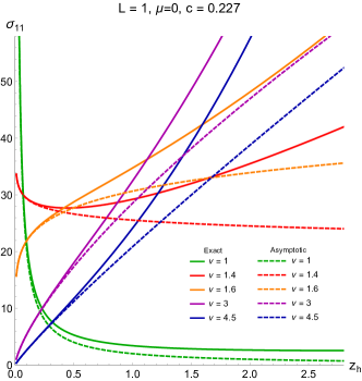
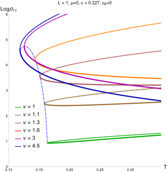
A              B

Figure 2: A) The dependence of the electric conductivity $\sigma^{11}$ on the size of horizon $z_{h}$ for different values of anisotropy parameter $\nu$ and zero magnetic field $c_{B}=0$. The solid lines show exact calculations, while dashed correspond to asymptotics around $z_{h}=0$. B) The dependence of electric conductivity $\sigma^{11}$ on the temperature $T$ for different values of anisotropy parameter $\nu$ and $\mu=0$ in logarithmic coordinates. The blue dot-dashed line presents the Hawking-Page phase transition points. Dashed lines represent values of $\sigma^{11}$ calculated in thermodynamically unstable phase.

In Fig.2.B the dependence of electric conductivity $\sigma^{11}$ on the temperature $T$ for $\mu=0$ and different values of anisotropy parameter $\nu$ is shown in logarithmic coordinates. In this case the electric conductivity $\sigma^{11}$ exists only in a certain temperature range due to phase transitions structure [29]. The Hawking-Page transition points are the leftmost points of curves when chemical potential is zero. For temperatures below the Hawking-Page transition, the conductivity should be calculated in thermal AdS. $\sigma^{11}$ on this plot is presented for calculations in the AdS black hole. We expect a phase transition at $T=T_{HP}$. The blue dot-dashed line presents the Hawking-Page phase transition points. Dashed lines represent values of $\sigma^{11}$ calculated in thermodynamically unstable phase.

Unlike $\sigma^{11}$, the 33-component of conductivity does not exhibit the change of asymptotic behavior near the horizon. Instead of (4.2), one has near $z_{h}=0$

$$\sigma^{33}\sim z_{h}^{\frac{0.816\sqrt{\nu-1}}{\nu}-1}.$$ (4.3)

The power of $z_{h}$ is always negative for $\nu\in[1,4.5]$ taking the maximum value of $-0.592$ for $\nu=2$. Therefore, $\sigma^{33}(z_{h})$ monotonously decreases for all considered values of $\nu$.

Plots of $\sigma^{11}(T)$ and $\sigma^{33}(T)$ are presented in Table 1 for different values of magnetic field parameter, chemical potential and anisotropy. We would like to mention the discontinuous behaviour of the conductivity as a function of temperature. We observe a jump at the temperature of Hawking-Page phase transition, which disappears as the magnetic field and chemical potential increase.

4.2 The lattice data fit for zero chemical potential

To fit the lattice results for zero chemical potential, we use the gauge kinetic function $f_{0}(\phi)$. This function couples Maxwell field to dilaton and depends on the size of horizon $z_{h}$, anisotropy parameter $\nu$ and magnetic field parameter $c_{B}$. The choice of this function is purely phenomenological. To get the fit presented in Fig.3, we take the kinetic function $f_{0}$ as

$$f_{0}(\phi) = \frac{1}{440}\left\{\left(\exp\left[-\frac{1}{10}\left(\phi(z_{h},\nu,c_{B})^{3}+\phi(z_{h},\nu,c_{B})\right)\right]+0.3\exp\left[-\frac{1}{30}\phi(z_{h},\nu,c_{B})^{2}\right]\right)+\right.$$ (4.4)

$$\left.\qquad+\frac{1}{15}\exp\left[-\frac{1}{0.04}\phi(z_{h}-z_{h}^{s},\nu,c_{B})^{2}\right]\right\},$$

where $z_{h}^{s}$ is a value that shifts the last Gaussian term to the point, where stable and unstable phases meet each other. It is necessary because two branches of the stable phase are widely separated in terms of $z_{h}$ but close to each other as functions of $T$.

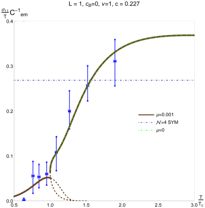
Figure 3: The dependence of ratio $\sigma^{11}/T$ on the temperature $T$ normalized by the critical value $T_{c}=0.163$ corresponding to the Hawking-Page phase transition is presented. The solid brown line corresponds to the stable phase with a small non-zero chemical potential $\mu=0.001$ while the green dash-dotted line represents the $\mu=0$ case. The blue dash-dotted line is $\mathcal{N}=4$ SYM conductivity $\sigma/T=e^{2}N_{c}^{2}/16\pi$. Blue dots correspond to lattice calculations from [50] for $N_{c}=N_{f}=3$.

In Fig.3 the dependence of ratio $\sigma^{11}/T$ on the temperature $T$ normalized by the critical value $T_{c}=0.163$ corresponding to the Hawking-Page phase transition is presented. The solid brown lines correspond to the stable phase with a small non-zero chemical potential $\mu=0.001$ while the green dash-dotted line represents the $\mu=0$ case. One can see that these two curves coincide in the region $T>T_{c}$, but the green one is not defined below $T_{c}$. The blue dash-dotted line is $\mathcal{N}=4$ SYM conductivity $\sigma/T=e^{2}N_{c}^{2}/16\pi$. $C_{em}^{-1}=\dfrac{2e^{2}}{3}$ is electromagnetic constant for number of flavors $N_{f}=3$ and colors $N_{c}=3$. Blue dots with error bars correspond to lattice calculations from [50] for $N_{c}=N_{f}=3$. Although the lattice calculations are made for light quarks (u,d,s), the pion mass is $M_{\pi}=384$ MeV, which is almost 3 times bigger than its physical mass. In addition, the ratio $M_{\pi}/M_{\rho}$ is 3 times bigger. This obstacle indicates that there are yet no reliable lattice results for both heavy and light quarks. Either way, we use these data to adjust the coupling $f_{0}(\phi)$ so that in a simple case of vanishing chemical potential and zero magnetic field, the electric conductivity in our model fits lattice results. We have already mentioned that our model’s ansatz corresponds to the case of heavy quarks, so in general, $\sigma$ does not have to agree with these data. Once $f_{0}(\phi)$ is tuned, it is possible to predict the behaviour of $\sigma$ for different parameters of the magnetic field, anisotropy and chemical potential. In this work, we define the dilaton coupling as in (4.4).

Plots of $f_{0}$ as a function of both $z_{h}$ and $T$ are presented on Fig.4 for different sets of parameters. As one can see on Fig.4.A there is a hump near $z_{h}\approx 10$. It corresponds to the rise of the stable phase of $\sigma^{11}/T$ in the $\frac{T}{T_{c}}\in[0.5,1.0]$ region in Fig.3. Also note, that $f_{0}$ does not depend on the chemical potential $\mu$. Thus, all the model’s predictions about the impact of finite chemical potential are independent of a particular choice of kinetic function.

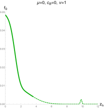
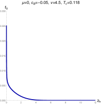
A                                                              B
 
      
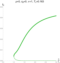
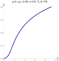
C                                                              D

Figure 4: The dependence of our choice of $f_{0}$ function (4.4) on the size of the horizon (A,B) and on the temperature $T/T_{c}$ (C,D) for isotropic case (green curves) and anisotropic one (dark blue curves).

4.3 Quadratic approximation of conductivity dependence for small chemical potential

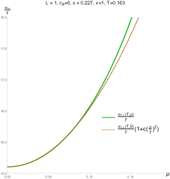
Figure 5: The dependence of $\sigma^{11}/T$ on the chemical potential $\mu$ for temperature $T=0.163$ corresponding to the Hawking-Page phase transition. The green curve represents the exact answer, the dashed brown curve is the power series in $\mu$ around $\mu=0$.

Symmetries of the QCD action imply the evenness of $\sigma/T$ as a function of chemical potential. Therefore its power series may contain only even powers of $\mu$:

$$\dfrac{\sigma(T,\mu)}{T}=\dfrac{\sigma(T,0)}{T}\left(1+c(T)\left(\dfrac{\mu}{T}\right)^{2}+O\left(\mu^{4}\right)\right).$$ (4.5)

This quadratic dependence has been studied in numerous works using lattice calculations [52], and different phenomenological models [66]. It was shown, that the function $c(T)$ remains constant for quite a wide range of temperatures around the phase transition. In our case, the best match of the two curves occurs for $c(T)\approx 0.16$, which agrees with [52]. The plot Fig.5 shows an adequate behaviour of the electric conductivity in our model, consistent with the conventional understanding of this phenomenon. This plot is also a clear illustration of independence of the function $f_{0}$ of chemical potential. It follows from the Einstein equations for model [29] that the dilaton field does not depend on the chemical potential. Since the gauge kinetic function $f_{0}(\phi)$ depends on the dilaton only, the $f_{0}$ in the ratio $\sigma/T$ in Fig.5 remains constant for all values of $\mu$. Thus, the qualitative behaviour is right despite of the particular choice of the gauge kinetic function.

4.4 Calculation of $\sigma^{11}$

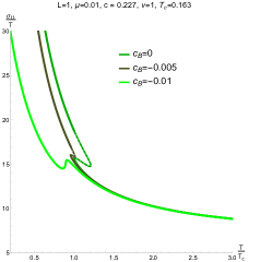
A                                     B                                    C

Figure 6: A) The dependence of $\sigma^{11}$ on the temperature $T$ is presented with the dilaton coupling $f_{0}(\phi)=1$. B) The dependence of the ratio $\sigma^{11}/T$ on the temperature $T$ is presented with the dilaton coupling $f_{0}(\phi)=1$. C) The electric conductivity comes with $f_{0}(\phi)$ function from (4.4). The plot-in shows the zoom of the main plot near the jumps.

In Fig.6.A and Fig.6.B the dependence of conductivity $\sigma^{11}$ and ratio $\sigma^{11}/T$ on the temperature $T$ are presented with the gauge kinetic function $f_{0}(\phi)=1$. In Fig.6.C the electric conductivity comes with $f_{0}(\phi)$ function from (4.4). The addition of the dilaton coupling changes the behaviour of the conductivity dramatically both below and above the critical value of temperature $T_{c}$. But some important physical features remain invariant of the kinetic function, i.e. the positions of conductivity’s jumps and the dependence on chemical potential and magnetic field. Roughly speaking, the greater the chemical potential or/and magnetic field, the smoother the conductivity. For some values of parameters the unstable phase vanishes. This happens when the temperature as a function of $z_{h}$ ceases to be three-critical. Also, the $\mu$-dependent effects are invariant to the choice of the coupling function.

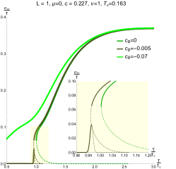
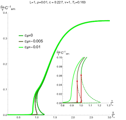
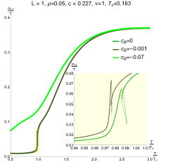
A                                             B                                             C
 
   
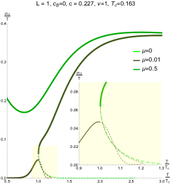
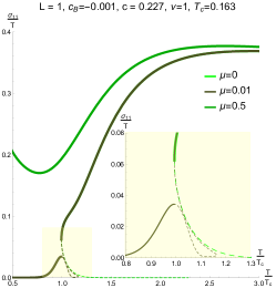
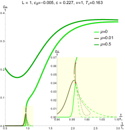
D                                             E                                             F

Figure 7: The dependence of $\sigma^{11}/T$ on the normalized temperature $T/T_{c}$ for different values of magnetic field’s parameter $c_{B}$ and $\mu=0$ (A), $\mu=0.01$ (B) and $\mu=0.05$ (C), and for different values of chemical potential $\mu$ and $c_{B}=0$ (D), $c_{B}=-0.001$ (E) and $c_{B}=-0.005$ (F). Here $\nu=1$. Dashed lines represent values of $\sigma^{11}$ calculated in thermodynamically unstable phase. The built-in graphs show the zoom of the main plots near the jumps.

In Fig.7 the ratio of electric conductivity to temperature $\sigma^{11}/T$ on the normalized temperature $T/T_{c}$ for $\nu=1$ and different values of magnetic field’s parameter $c_{B}$ and chemical potential $\mu$ with the coupling function $f_{0}(\phi)$ given by (4.4) are presented. One can see the BB phase transition, which appears at the temperature $T_{BB}(\nu,c_{B},\mu)$. At this temperature, the electric conductivity has a jump. Increasing the chemical potential and/or magnetic field implies vanish of the jump. At ultra-high temperatures, curves on Fig.7 are approaching some constant value between $0.3$ and $0.31$ that is the same for all parameters. This asymptotic value can be adjusted with an overall factor in $f_{0}$ function.

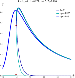
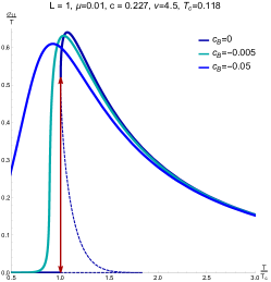
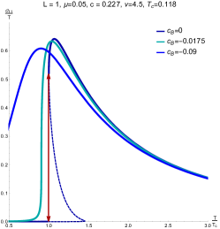
A                                             B                                             C
 
   
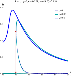
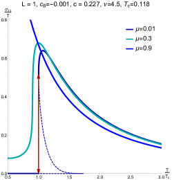
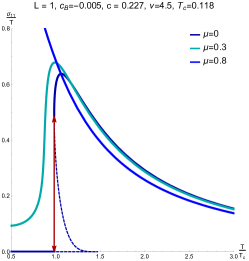
D                                             E                                             F

Figure 8: The dependence of $\sigma^{11}/T$ on the normalized temperature $T/T_{c}$ for different values of magnetic field’s parameter $c_{B}$ and $\mu=0$ (A), $\mu=0.01$ (B) and $\mu=0.05$ (C), and for different values of chemical potential $\mu$ and $c_{B}=0$ (D), $c_{B}=-0.001$ (E) and $c_{B}=-0.005$ (F). Here $\nu=4.5$. The dashed lines represent values of $\sigma^{11}$ calculated in thermodynamically unstable phase.

In Fig.8 the ratio of electric conductivity to temperature on the normalized temperature $T/T_{c}$ for $\nu=4.5$ and different values of magnetic field’s parameter $c_{B}$ and chemical potential $\mu$ with the coupling function $f_{0}(\phi)$ given by (4.4) are presented. We can see the BB phase transition which appears at the temperature $T_{BB}(\nu,c_{B},\mu)$. At this temperature, the electric conductivity has a jump. Increasing the chemical potential and/or magnetic field implies vanish of the jump. For ultra high values of chemical potential we see that $\sigma^{11}/T$ monotonically decreases. Also note a significant change of behaviour of $\sigma^{11}/T$ for different $\nu$. For $\nu=1$ the curves increase after the phase transition and take some constant value around the SYM one for large temperatures. The opposite happens to $\nu=4.5$ case. The maximum value is reached near the point of phase transition and then the conductivity goes down, asymptotically approaching zero. This is the consequence of the change in asymptotic behaviour that we have mentioned in (4.2). The plot Fig.2 gives more detailed information about this phenomenon. The DC conductivity becomes so small for large $T$, that the QGP is almost opaque along the heavy-ions collision line.

4.5 Calculation of $\sigma^{33}$

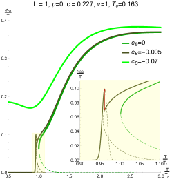
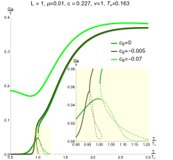
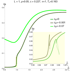
A                                             B                                             C
 
   
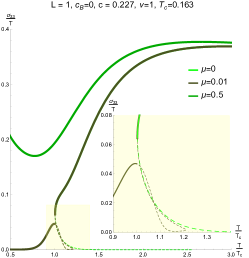
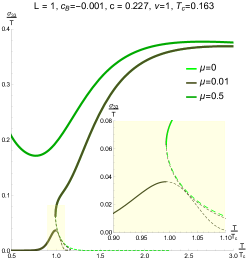
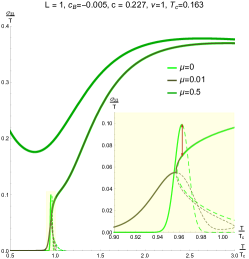
D                                             E                                             F

Figure 9: The dependence of $\sigma^{33}/T$ on the normalized temperature $T/T_{c}$ for different values of magnetic field’s parameter $c_{B}$ and $\mu=0$ (A), $\mu=0.01$ (B) and $\mu=0.05$ (C), and for different values of chemical potential $\mu$ and $c_{B}=0$ (D), $c_{B}=-0.001$ (E) and $c_{B}=-0.005$ (F). Here $\nu=1$. Dashed lines represent values of $\sigma^{11}$ calculated in thermodynamically unstable phase. The built-in graphs show the zoom of the main plots near the jumps.

In Fig.9 the ratio of electric conductivity to temperature $\sigma^{33}/T$ on the normalized temperature $T/T_{c}$ for $\nu=1$ and different values of magnetic field’s parameter $c_{B}$ and chemical potential $\mu$ with the coupling function $f_{0}(\phi)$ given by (4.4) are presented. We can see the BB phase transition which appears at the temperature $T_{BB}(\nu,c_{B},\mu)$. At this temperature the electric conductivity has a jump. Increasing the chemical potential and/or magnetic field implies vanish of the jump.

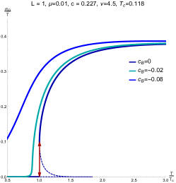
A                                             B                                             C
 
   
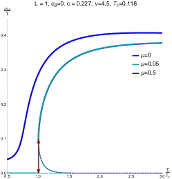
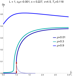
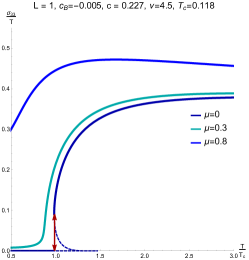
D                                             E                                             F

Figure 10: The dependence of $\sigma^{33}/T$ on the normalized temperature $T/T_{c}$ for different values of magnetic field’s parameter $c_{B}$ and $\mu=0$ (A), $\mu=0.01$ (B) and $\mu=0.05$ (C), and for different values of chemical potential $\mu$ and $c_{B}=0$ (D), $c_{B}=-0.001$ (E) and $c_{B}=-0.005$ (F). Here $\nu=4.5$. Dashed lines represent values of $\sigma^{33}$ calculated in thermodynamically unstable phase.

In Fig.10 the ratio of electric conductivity to temperature $\sigma^{33}/T$ on the normalized temperature $T/T_{c}$ for $\nu=4.5$ and different values of magnetic field’s parameter $c_{B}$ and chemical potential $\mu$ with the dilaton coupling function $f_{0}(\phi)$ given by (4.4) are presented. We can see the BB phase transition which appears at the temperature $T_{BB}(\nu,c_{B},\mu)$. At this temperature the electric conductivity has a jump. Increasing the chemical potential and/or magnetic field implies vanish of the jump.

4.6 Comparison of $\sigma^{22}$ and $\sigma^{33}$

It is interesting to note that $\sigma^{22}$ and $\sigma^{33}$ are not very different, see Fig.11.

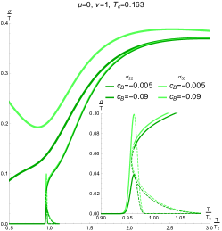
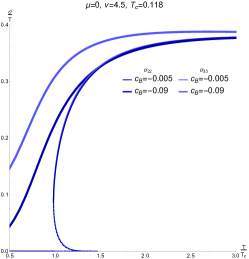
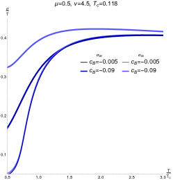
A                                             B                                             C

Figure 11: The dependence of $\sigma^{22}/T$ and $\sigma^{33}/T$ on the normalized temperature $T/T_{c}$ for different values of magnetic field’s parameter $c_{B}$ and $\mu=0$ (A, B), $\mu=0.05$ (C). Here $\nu=1$ on (A), and $\nu=4.5$ on (B) and (C). Dashed lines represent values of the conductivity calculated in thermodynamically unstable phase. The inset in (A) shows jumps near the critical points.

We see that, conductivities $\sigma^{22}$ and $\sigma^{33}$ are indistinguishable for small values of an external magnetic field (thin lines are almost indistinguishable in Fig.11). Neither anisotropy nor chemical potential can remove this degeneracy. It is clear from the definition of the anisotropy functions (2.3) and the expressions for conductivities (3.20)-(3.18). The anisotropy-dependant factors cancel out, and the magnetic field’s parameter enters these expressions with different signs. Therefore, the magnetic field tends to push the conductivities in different directions: $\sigma^{33}$ rises, and $\sigma^{22}$ goes down. All the other thermodynamic properties of these two values are the same.

 

5 Conclusion and Discussion

We have got that formulas (3.18), (3.19) and (3.20) give the electric conductivity for anisotropic holographic models. These formulas can be presented in a uniform way as

$$\sigma^{ii} = f_{0}\,g^{ii}\sqrt{\det g^{(3)}_{jk}}\,\Big{|}_{z=z_{h}},\qquad i,j,k=1,2,3,$$ (5.1)

where $g^{(3)}_{jk}$ is the spatial part of the diagonal metric (2.2). Noticing that the last multiplayer in (5.1) is nothing but the density of the entropy obtained in the case of the absence of the dynamical wall [68], in the terminology of [41], we can rewrite (5.1) as

$$\sigma^{ij} = f_{0}\,g^{ii}\,\Big{|}_{z=z_{h}}\,s,\qquad i=1,2,3,$$ (5.2)

where $s$ is the entropy density. It would be interesting to compare the dependence of the DC conductivity (3.18)–(3.20) on the anisotropy functions $\mathfrak{g}_{i}$ with other characteristics of anisotropic plasma [39]; in particular, with the string tensions and the drag forces calculated for model (2.1) in [29, 71, 72, 73]. It is convenient to write these quantities in terms of vierbeins

$${\bf e}^{a} = e_{\mu}^{a}(z)dx^{\mu},\quad a=0,1,...3,\quad\mu=0,1,...3,$$ (5.3)

$$e_{\mu}^{a}(z) = \delta_{\mu}^{a}\,\sqrt{\frac{\mathfrak{b}}{z^{2}}\,\mathfrak{g}_{\mu}},\quad\mathfrak{g}_{0}=g,\,\,g_{\mu\nu}=\eta_{ab}e_{\mu}^{a}e_{\nu}^{b},$$

$\eta_{ab}$ is the Minkowski metric. In particular, in the absence of the dynamical wall, the tension of the Wilson loop lying on a (regularized) boundary and extending in the spatial directions $(i,j)$ is

$$\bm{\tau}^{ab} = {\bf e}(z)^{a}\wedge{\bf e}(z)^{b}\Big{|}_{z=z_{h}},$$ (5.4)

$$\tau^{ab}_{\mu\nu} = e(z)^{a}_{\mu}e(z)^{b}_{\nu}=\delta_{\mu}^{a}\delta_{\nu}^{b}\frac{b}{z^{2}}\sqrt{\,\mathfrak{g}_{\mu}\,\mathfrak{g}_{\nu}}\Big{|}_{z=z_{h}}.$$ (5.5)

For the drag forces in anizotropic models we have got [71]

$$f_{i}=g_{ii}\Big{|}_{z=z_{h}}\,v^{i},\quad i=1,2,3,$$ (5.6)

here $v^{i}$ is a constant velocity.

We have numerically studied the dependence of the electric conductivity on the anisotropy parameter, temperature, magnetic field, and chemical potential within the holographic anisotropic QGP model [29]. Plots of the electric conductivity vs temperature are presented in the summary Table 1. Here the gauge kinetic function is set to 1, $f_{0}=1$.

We use freedom of choice of the gauge kinetic function to reproduce the lattice results for small chemical potential, magnetic field and isotropic medium. Then, we calculate the conductivity with $f_{0}$ from (4.4). The results are summarized in Table 2. The most essential consequences are

• at high temperatures the ratios $\sigma^{ii}/T$, $i=2,3$ (orthogonal to the collision line directions) go to the same constant value which is defined by the choice of $f_{0}$ function. Meanwhile, the $\sigma^{11}/T$ goes to zero. The DC conductivity becomes so small for large $T$, that the QGP is almost opaque along the heavy-ion collision line;

• near the phase transition

  • the DC conductivity experiences a jump for small or zero values of chemical potential and magnetic field for both isotropic and anisotropic cases;

  • increasing the chemical potential and/or magnetic field smoothens the curves, and for high enough parameters the jump disappears;

  • generally, the phase transition is of the first order, but it happens to become the second order for some very special set of parameters;

• conductivities $\sigma^{22}$ and $\sigma^{33}$ are indistinguishable for small values of an external magnetic field. Neither anisotropy nor chemical potential can remove this degeneracy.

Note that the DC conductivity characterises static low frequency fluctuations of the system. Recently, the butterfly velocity [74, 75], that shows how fast chaotic correlations propagate in the plasma, has been studied in holographic anisotropic models [30]. It has been observed that it exhibits a rich structure as a function of temperature, anisotropy and magnetic field and exceeds the conformal value in certain regimes. It would be interesting to investigate the butterfly’s velocity for the model considered here [29] and for the light quarks holographic model [28]. Interplane between DC conductivity and butterfly velocity over an anisotropic background has been considered recently in [76].

We also plan to consider more general ansatz of a plane electromagnetic wave and to investigate the dependence of differential photon emission rate on anisotropy parameter, temperature and chemical potential, as well to use directly the holographic model for light quarks, that supposed to be a generalization for the twice anisotropic case of the model considered in [28].

 

6 Acknowledgments

We would like to thank K.Rannu for useful discussions. A.E. would like to thank A. Starinets for correspondence. This work is supported by Russian Science Foundation grant 20-12-00200.

 

Appendix

Appendix A Retarded Green’s functions approach

To evaluate polarization operators, one has to write the on-shell action in momentum space. Therefore we Fourier transform fields as

$$A_{\mu}(z,\vec{x},t)=\int\frac{d^{4}k}{(2\pi)^{4}}e^{-i(wt-\vec{k}\vec{x})}A_{\mu}(z,w,k).$$ (A.1)

Also, we decompose

$$E_{i}(w,k,z)=w\mathcal{E}_{i}(w,k)\psi_{i}(z),\quad\mbox{for}\quad i=1,2,3,$$ (A.2)

where $\psi_{i}(z)\rightarrow 1$ as $z\rightarrow 0$ [14].

The surface term (2.6) in momentum space then takes the following form

$$S_{sur\!f}=\int\frac{d^{4}k}{(2\pi)^{4}}\frac{f_{0}\,g}{z}\sqrt{\mathfrak{b}\,\mathfrak{g}_{1}\mathfrak{g}_{2}\mathfrak{g}_{3}}\left(-\mathcal{E}_{3}(-k,-w)\frac{\psi_{3}^{*}\psi_{3}^{\prime}}{\frac{k^{2}}{w^{2}}g-\mathfrak{g}_{3}}\mathcal{E}_{3}(k,w)+\right.$$

$$\left.\left.+\mathcal{E}_{1}(-k,-w)\frac{\psi_{1}^{*}\psi_{1}^{\prime}}{\mathfrak{g}_{1}}\mathcal{E}_{1}(k,w)+\mathcal{E}_{2}(-k,-w)\frac{\psi_{2}^{*}\psi_{2}^{\prime}}{\mathfrak{g}_{2}}\mathcal{E}_{2}(k,w)\right)\right|_{z=0}^{z=z_{h}}.$$ (A.3)

2-point Green’s functions are defined from the action (A) as

$$G^{\mu\nu}(k_{1},\omega_{1};k_{2},\omega_{2})=\frac{\delta^{2}S_{sur\!f}}{\delta\mathcal{E}_{\mu}(k_{1},\omega_{1})\delta\mathcal{E}_{\nu}(k_{2},\omega_{2})}.$$ (A.4)

To calculate Green’s functions one has to know functions $\psi$ on both the horizon and the boundary. These functions satisfy equations of motion for Maxwell field in the bulk. Furthermore, one needs physically reasonable boundary conditions to fix these solutions. To overcome these obstacles, we are following the prescription from [14]. According to it, one has to find asymptotic solutions to EOMs which are constant on the boundary and satisfy the in-falling conditions on the horizon. One then obtains the on-shell action in the form

$$S=\int\left.\frac{d^{4}k}{(2\pi)^{4}}J(-k)\mathcal{F}(z,k)J(k)\right|_{z=0}^{z=z_{h}}.$$ (A.5)

Following [15] the retarded Green’s function is

$$G_{R}(k)=-2\lim_{z\rightarrow 0}\mathcal{F}(z,k),$$ (A.6)

and its imaginary part as in [14] can be represented as

$$\mbox{Im}G_{R}(k)=-2\lim_{z\rightarrow z_{h}}\mbox{Im}\mathcal{F}(z,k).$$ (A.7)

To calculate retarded Green’s functions we plug the decomposition (A.2) into (3)-(3.7) and investigate asymptotics at $z=0$ and $z=z_{h}$.

We assume that the asymptotic value of the blackening function on the boundary is

$$g(z)=1+o(z);$$ (A.8)

while on the horizon is

$$g(z)=g^{\prime}(z_{h})(z_{h}-z)+o(z_{h}-z).$$ (A.9)

A.1 Transverse components of electric field

First, we find asymptotics for (3.6)

$$\psi_{1}^{\prime\prime}+\psi_{1}^{\prime}\left(\dfrac{\mathfrak{b}^{\prime}}{2\mathfrak{b}}+\dfrac{f_{0}^{\prime}}{f_{0}}+\dfrac{g^{\prime}}{g}+\dfrac{\mathfrak{g}_{2}^{\prime}}{2\mathfrak{g}_{2}}+\dfrac{\mathfrak{g}_{3}^{\prime}}{2\mathfrak{g}_{3}}-\dfrac{\mathfrak{g}_{1}^{\prime}}{2\mathfrak{g}_{1}}-\dfrac{1}{z}\right)+\psi_{1}\dfrac{w^{2}\mathfrak{g}_{3}-k^{2}g}{g^{2}\mathfrak{g}_{3}}=0.$$ (A.10)

The requirement $\psi_{i}\rightarrow 1$ near the boundary is consistent with equations of motion. Its’ asymptotic behaviour near the boundary $z=0$ takes the form

$$\psi_{1}^{\prime\prime}-\frac{\psi_{1}^{\prime}}{z}=0.$$ (A.11)

Its solution is simply

$$\psi_{1}=C_{1}+C_{2}z^{2}.$$ (A.12)

Near the horizon (A.10) has singularities of $1/g$ terms. So the equation for asymptotic behaviour on the horizon

$$\psi_{1}^{\prime\prime}-\frac{1}{z_{h}-z}\psi_{1}^{\prime}+\frac{w^{2}}{g^{\prime}(z_{h})^{2}(z_{h}-z)^{2}}\psi_{1}=0.$$ (A.13)

The solution for this equation is a linear combination of two linear independent solutions

$$\psi_{1}(z)= c_{1}\cos\left(\frac{w}{g^{\prime}(z_{h})}\ln(z_{h}-z)\right)+c_{2}\sin\left(\frac{w}{g^{\prime}(z_{h})}\ln(z_{h}-z)\right)=$$ (A.14)

$$=\frac{1}{2}(c_{1}+ic_{2})(z_{h}-z)^{-i\frac{w}{g^{\prime}(z_{h})}}+\frac{1}{2}(c_{1}-ic_{2})(z_{h}-z)^{i\frac{w}{g^{\prime}(z_{h})}}.$$

Both these solutions oscillate and are finite near the horizon. We will call the first one $f_{k^{\mu}}=(z_{h}-z)^{-i\frac{w}{g^{\prime}(z_{h})}}$ and the second one as its complex conjugate $f_{-k^{\mu}}$. If one also restores time-dependent part $e^{-iwt}$, then

$$e^{-iwt}f_{k^{\mu}}=e^{-iw(t+z_{*})},$$ (A.15)

where $z_{*}=\frac{\ln(z_{h}-z)}{g^{\prime}(z_{h})}$. Therefore $f_{k^{\mu}}$ describes the incoming (that moves towards the horizon) wave, whilst $f_{-k^{\mu}}$ corresponds to outgoing wave. The boundary condition on the horizon requires choosing the incoming wave only since no signal can escape from a black hole. So we have

$$\mathcal{F}(z,k)=\frac{f_{0}g}{z}\sqrt{\frac{\mathfrak{b}\,\mathfrak{g}_{3}\mathfrak{g}_{2}}{\mathfrak{g}_{1}}}f_{-k^{\mu}}\frac{df_{k^{\mu}}}{dz}=\frac{f_{0}g}{z}\sqrt{\frac{\mathfrak{b}\,\mathfrak{g}_{3}\mathfrak{g}_{2}}{\mathfrak{g}_{1}}}\frac{iw}{g^{\prime}(z_{h})}\frac{1}{z_{h}-z}.$$ (A.16)

$$\mbox{Im}\,G_{R}^{11} = -2\lim_{z\rightarrow z_{h}}\frac{f_{0}(z)g(z)}{z}\sqrt{\frac{\mathfrak{b}(z)\,\mathfrak{g}_{3}(z)\mathfrak{g}_{2}(z)}{\mathfrak{g}_{1}(z)}}\frac{w}{g^{\prime}(z_{h})(z_{h}-z)}$$ (A.17)

$$= -2wf_{0}(z_{h})\sqrt{\frac{\mathfrak{b}(z_{h})\mathfrak{g}_{3}(z_{h})\mathfrak{g}_{2}(z_{h})}{\mathfrak{g}_{1}(z_{h})z^{2}_{h}}}.$$

And using the Kubo formula $\sigma^{\mu\nu}=-G^{\mu\nu}_{R}/iw$ we obtain the 11-component of QGP electric conductivity tensor to be nothing but (3.19). Doing all the same we obtain the 22-component of QGP electric conductivity to be (3.20).

A.2 Longitudinal component of electric field

From the on-shell action (A) the longitudinal part reads

$$S_{sur\!f}=\int\frac{d^{4}k}{(2\pi)^{4}}f_{0}\frac{g}{z}\mathcal{E}_{3}(-k,-w)\psi_{3}^{*}\psi_{3}^{\prime}\mathcal{E}_{3}(k,w)\frac{\sqrt{\mathfrak{b}\mathfrak{g}_{3}\mathfrak{g}_{2}\mathfrak{g}_{1}}}{\mathfrak{g}_{3}-g\frac{k^{2}}{w^{2}}},$$ (A.18)

and the equation of motion (3)

$$\psi_{3}^{\prime\prime}+\psi_{3}^{\prime}\left(\dfrac{\mathfrak{b}^{\prime}}{2\mathfrak{b}}+\dfrac{f_{0}^{\prime}}{f_{0}}-\dfrac{w^{2}\mathfrak{g}_{3}g^{\prime}}{k^{2}g^{2}-w^{2}g\mathfrak{g}_{3}}+\dfrac{w^{2}\mathfrak{g}_{3}^{\prime}}{k^{2}g-w^{2}\mathfrak{g}_{3}}+\dfrac{\mathfrak{g}_{1}^{\prime}}{2\mathfrak{g}_{1}}+\dfrac{\mathfrak{g}_{2}^{\prime}}{2\mathfrak{g}_{2}}+\dfrac{\mathfrak{g}_{3}^{\prime}}{2\mathfrak{g}_{3}}-\dfrac{1}{z}\right)+$$

$$+\psi_{3}\dfrac{w^{2}\mathfrak{g}_{3}-k^{2}g}{g^{2}\mathfrak{g}_{3}}=0.$$ (A.19)

To find the asymptotic behaviour of the solution to this equation near the horizon, we make the same assumptions about functions as in the previous section (A.8), (A.9). Then the equation in the vicinity of horizon is

$$\psi_{3}^{\prime\prime}+\frac{\psi_{3}^{\prime}}{(z-z_{h})}+\frac{w^{2}}{(g^{\prime}(z_{h}))^{2}(z-z_{h})^{2}}\psi_{3}=0.$$ (A.20)

Its’ solution is

$$\psi_{3}(z)=c_{1}(z_{h}-z)^{-\frac{iw}{g^{\prime}(z_{h})}}+c_{2}(z_{h}-z)^{\frac{iw}{g^{\prime}(z_{h})}}.$$ (A.21)

Where we as before imply the infalling boundary condition, eliminating the outgoing wave.

$$\psi_{3}(z)\sim(z_{h}-z)^{-iw/g^{\prime}(z_{h})}.$$ (A.22)

Then the imaginary part of the retarded Green’s function is

$$\mathrm{Im}G_{R}^{33}=-2\lim_{z\rightarrow z_{h}}\mathrm{Im}\left[\frac{f_{0}g}{z}\frac{\sqrt{b\,\mathfrak{g}_{1}\mathfrak{g}_{2}\mathfrak{g}_{3}}}{\mathfrak{g}_{3}-g\frac{k^{2}}{w^{2}}}\psi_{3}^{*}\frac{d\psi_{3}}{dz}\right]$$ (A.23)

In the $z\rightarrow z_{h}$ limit we use the obtained asymptotic behaviour of $\psi_{3}$

$$\psi_{3}^{*}\frac{d\psi_{3}}{dz}=\frac{iw}{g^{\prime}(z_{h})(z_{h}-z)}.$$ (A.24)

The result then follows from the Kubo relation (3.18).
Note, all the obtained results completely agree with another approach from Sect. 3 and reduce to that of isotropic and partially anisotropic models.

Appendix B Tables for conductivities

Table 1: Table shows the dependence of the DC conductivity on anisotropy, chemical potential and magnetic field. Here $f_{0}=1$.

Table 2: Table shows dependencies of the ration of the DC conductivity to temperature on anisotropy, chemical potential and magnetic field. Here $f_{0}$ is given by (4.4)

References

- [1] G. David, “Direct real photons in relativistic heavy ion collisions,” Rept. Prog. Phys. 83, no.4, 046301 (2020) [arXiv:1907.08893 [nucl-ex]].
- [2] S. Caron-Huot, P. Kovtun, G. D. Moore, A. Starinets and L. G. Yaffe, “Photon and dilepton production in supersymmetric Yang-Mills plasma,” JHEP 12, 015 (2006) [arXiv:hep-th/0607237 [hep-th]].
- [3] J. Casalderrey-Solana, H. Liu, D. Mateos, K. Rajagopal and U. A. Wiedemann, “Gauge/String Duality, Hot QCD and Heavy Ion Collisions”, Cambridge University Press (2014) [arXiv:1101.0618 [hep-th]].
- [4] I. Ya. Aref’eva, “Holographic approach to quark-gluon plasma in heavy ion collisions”, Phys. Usp. 57, 527 (2014).
- [5] O. DeWolfe, S. S. Gubser, C. Rosen and D. Teaney, “Heavy ions and string theory”, Prog. Part. Nucl. Phys. 75, 86 (2014) [arXiv:1304.7794 [hep-th]].
- [6] L. Patino and D. Trancanelli, “Thermal photon production in a strongly coupled anisotropic plasma,” JHEP 02, 154 (2013) [arXiv:1211.2199 [hep-th]].
- [7] S. Y. Wu and D. L. Yang, “Holographic Photon Production with Magnetic Field in Anisotropic Plasmas,” JHEP 08, 032 (2013) [arXiv:1305.5509 [hep-th]].
- [8] S. I. Finazzo and J. Noronha, “Holographic calculation of the electric conductivity of the strongly coupled quark-gluon plasma near the deconfinement transition,” Phys. Rev. D 89, no.10, 106008 (2014) [arXiv:1311.6675 [hep-th]].
- [9] G. Arciniega, F. Nettel, P. Ortega and L. Patiño, “Brighter Branes, enhancement of photon production by strong magnetic fields in the gauge/gravity correspondence,” JHEP 04, 192 (2014) [arXiv:1307.1153 [hep-th]].
- [10] I. Iatrakis, E. Kiritsis, C. Shen and D. Yang, “Holographic Photon Production in Heavy Ion Collisions,” JHEP 04, 035 (2017) [arXiv:1609.07208 [hep-ph]].
- [11] I. Aref’eva, “Holography for Heavy Ions Collisions at LHC and NICA,” EPJ Web Conf. 164, 01014 (2017) [arXiv:1612.08928 [hep-th]].
- [12] D. Ávila, T. Monroy, F. Nettel and L. Patiño, “Emission of linearly polarized photons in a strongly coupled magnetized plasma from the gauge/gravity correspondence,” Phys. Lett. B 817, 136287 (2021) [arXiv:2101.08802 [hep-th]].
- [13] D. T. Son and A. O. Starinets, ‘Viscosity, Black Holes, and Quantum Field Theory,” Ann. Rev. Nucl. Part. Sci. 57, 95-118 (2007) [arXiv:0704.0240 [hep-th]].
- [14] D. T. Son and A. O. Starinets, “Minkowski space correlators in AdS / CFT correspondence: Recipe and applications,” JHEP 09, 042 (2002) [arXiv:hep-th/0205051 [hep-th]].
- [15] G. Policastro, D. T. Son and A. O. Starinets, “From AdS / CFT correspondence to hydrodynamics,” JHEP 09, 043 (2002) [arXiv:hep-th/0205052 [hep-th]].
- [16] N. Iqbal and H. Liu, “Universality of the hydrodynamic limit in AdS/CFT and the membrane paradigm,” Phys. Rev. D 79, 025023 (2009) [arXiv:0809.3808 [hep-th]].
- [17] M. Parikh and F. Wilczek, “An Action for black hole membranes,” Phys. Rev. D 58, 064011 (1998) [arXiv:gr-qc/9712077 [gr-qc]].
- [18] U. Gursoy, E. Kiritsis, L. Mazzanti, G. Michalogiorgakis and F. Nitti, “Improved Holographic QCD,” Lect. Notes Phys. 828, 79-146 (2011) [arXiv:1006.5461 [hep-th]].
- [19] S. He, S.-Y. Wu, Y. Yang and P.-H. Yuan, “Phase Structure in a Dynamical Soft-Wall Holographic QCD Model”, JHEP 04, 093 (2013) [arXiv:1301.0385 [hep-th]].
- [20] A. Donos and J. P. Gauntlett, “Thermoelectric DC conductivities from black hole horizons,” JHEP 11, 081 (2014) [arXiv:1406.4742 [hep-th]].
- [21] Y. Yang and P.-H. Yuan, “Confinement-deconfinement phase transition for heavy quarks in a soft wall holographic QCD model”, JHEP 1512, 161 (2015) [arXiv:1506.05930 [hep-th]].
- [22] D. Dudal and S. Mahapatra, “Thermal entropy of a quark-antiquark pair above and below deconfinement from a dynamical holographic QCD model”, Phys. Rev. D 96, no.12, 126010 (2017) [arXiv:1708.06995 [hep-th]].
- [23] D. Dudal and S. Mahapatra, “Interplay between the holographic QCD phase diagram and entanglement entropy”, JHEP 07, 120 (2018) [arXiv:1805.02938 [hep-th]].
- [24] S. Mahapatra, “Interplay between the holographic QCD phase diagram and mutual and -partite information”, JHEP 04, 137 (2019) [arXiv:1903.05927 [hep-th]].
- [25] U. Gürsoy, M. Järvinen, G. Nijs and J. F. Pedraza, “Inverse Anisotropic Catalysis in Holographic QCD”, JHEP 04, 071 (2019) [arXiv:1811.11724 [hep-th]].
- [26] H. Bohra, D. Dudal, A. Hajilou and S. Mahapatra, “Anisotropic string tensions and inversely magnetic catalyzed deconfinement from a dynamical AdS/QCD model”, Phys. Lett. B 801, 135184 (2020) [arXiv:1907.01852 [hep-th]]. [arXiv:2009.05562 [hep-th]].
- [27] J. Zhou, X. Chen, Y. Q. Zhao and J. Ping, “Thermodynamics of heavy quarkonium in a magnetic field background,” Phys. Rev. D 102, no.8, 086020 (2020) [arXiv:2006.09062 [hep-ph]].
- [28] I. Y. Aref’eva, K. Rannu and P. Slepov, “Holographic Anisotropic Model for Light Quarks with Confinement-Deconfinement Phase Transition,” JHEP 06, 090 (2021), [arXiv:2009.05562 [hep-th]].
- [29] I. Y. Aref’eva, K. Rannu and P. Slepov, “Holographic model for heavy quarks in anisotropic hot dense QGP with external magnetic field,” JHEP 07, 161 (2021) [arXiv:2011.07023 [hep-th]].
- [30] U. Gürsoy, M. Järvinen, G. Nijs and J. F. Pedraza, “On the interplay between magnetic field and anisotropy in holographic QCD,” JHEP 03, 180 (2021) [arXiv:2011.09474 [hep-th]].
- [31] S. He, Y. Yang and P. H. Yuan, “Analytic Study of Magnetic Catalysis in Holographic QCD”, [arXiv:2004.01965 [hep-th]].
- [32] H. Bohra, D. Dudal, A. Hajilou and S. Mahapatra, “Chiral transition in the probe approximation from an Einstein-Maxwell-dilaton gravity model,” Phys. Rev. D 103, no.8, 086021 (2021) [arXiv:2010.04578 [hep-th]].
- [33] A. Ballon-Bayona, J. P. Shock and D. Zoakos, “Magnetic catalysis and the chiral condensate in holographic QCD,” JHEP 10, 193 (2020) [arXiv:2005.00500 [hep-th]].
- [34] D. M. Rodrigues, D. Li, E. Folco Capossoli and H. Boschi-Filho, “Finite density effects on chiral symmetry breaking in a magnetic field in 2+1 dimensions from holography,” Phys. Rev. D 103, no.6, 066022 (2021) [arXiv:2010.06762 [hep-th]].
- [35] D. Dudal, A. Hajilou and S. Mahapatra, “A quenched 2-flavour Einstein–Maxwell–Dilaton gauge-gravity model,” Eur. Phys. J. A 57, no.4, 142 (2021) [arXiv:2103.01185 [hep-th]].
- [36] A. Ballon-Bayona, L. A. H. Mamani, A. S. Miranda and V. T. Zanchin, “Effective holographic models for QCD: Thermodynamics and viscosity coefficients,” Phys. Rev. D 104, no.4, 046013 (2021) [arXiv:2103.14188 [hep-th]].
- [37] N. G. Caldeira, E. Folco Capossoli, C. A. D. Zarro and H. Boschi-Filho, “Fluctuation and dissipation within a deformed holographic model at finite temperature and chemical potential,” [arXiv:2104.08397 [hep-th]].
- [38] J. Zhou and J. Ping, “Holographic Schwinger Effect in Anisotropic Media,” [arXiv:2101.08105 [hep-th]].
- [39] D. Giataganas, “Probing strongly coupled anisotropic plasma”, JHEP 1207, 031 (2012) [arXiv:1202.4436 [hep-th]].
- [40] D. S. Ageev, I. Y. Aref’eva, A. A. Golubtsova and E. Gourgoulhon, “Thermalization of holographic Wilson loops in spacetimes with spatial anisotropy,” Nucl. Phys. B 931, 506-536 (2018) [arXiv:1606.03995 [hep-th]].
- [41] I. Aref’eva and K. Rannu, “Holographic Anisotropic Background with Confinement-Deconfinement Phase Transition”, JHEP 1805, 206 (2018) [arXiv:1802.05652 [hep-th]].
- [42] I. Aref’eva, K. Rannu and P. Slepov, “Orientation Dependence of Confinement-Deconfinement Phase Transition in Anisotropic Media,” Phys. Lett. B 792, 470-475 (2019) [arXiv:1808.05596 [hep-th]].
- [43] I. Aref’eva, K. Rannu and P. Slepov, “Cornell potential for anisotropic QGP with non-zero chemical potential”, EPJ Web Conf. 222, 03023 (2019)
- [44] I. Y. Aref’eva and A. A. Golubtsova, “Shock waves in Lifshitz-like spacetimes”, JHEP 04, 011 (2015) [arXiv:1410.4595 [hep-th]].
- [45] X. H. Ge, S. J. Sin and S. F. Wu, “Universality of DC Electrical Conductivity from Holography,” Phys. Lett. B 767, 63-68 (2017) [arXiv:1512.01917 [hep-th]].
- [46] S. Khimphun, B. H. Lee and C. Park, “Conductivities in an anisotropic medium,” Phys. Rev. D 94, no.8, 086005 (2016) [arXiv:1604.00156 [hep-th]].
- [47] X. M. Kuang, E. Papantonopoulos, J. P. Wu and Z. Zhou, “Lifshitz black branes and DC transport coefficients in massive Einstein-Maxwell-dilaton gravity,” Phys. Rev. D 97, no.6, 066006 (2018) [arXiv:1709.02976 [hep-th]].
- [48] F. R. Brown, F. P. Butler, H. Chen, N. H. Christ, Z. h. Dong, W. Schaffer, L. I. Unger and A. Vaccarino, “On the existence of a phase transition for QCD with three light quarks,” Phys. Rev. Lett. 65, 2491-2494 (1990)
- [49] O. Philipsen and C. Pinke, “The QCD chiral phase transition with Wilson fermions at zero and imaginary chemical potential,” Phys. Rev. D 93, no.11, 114507 (2016) [arXiv:1602.06129 [hep-lat]].
- [50] G. Aarts, C. Allton, A. Amato, P. Giudice, S. Hands and J. I. Skullerud, “Electrical conductivity and charge diffusion in thermal QCD from the lattice,” JHEP 02, 186 (2015) [arXiv:1412.6411 [hep-lat]].
- [51] J. Ghiglieri, O. Kaczmarek, M. Laine and F. Meyer, “Lattice constraints on the thermal photon rate,” Phys. Rev. D 94, no.1, 016005 (2016) [arXiv:1604.07544 [hep-lat]].
- [52] P. V. Buividovich, D. Smith and L. von Smekal, “Electric conductivity in finite-density lattice gauge theory with dynamical fermions,” Phys. Rev. D 102, no.9, 094510, (2020) [arXiv:2007.05639 [hep-lat]].
- [53] G. Aarts and A. Nikolaev, “Electrical conductivity of the quark-gluon plasma: perspective from lattice QCD,” Eur. Phys. J. A 57, no.4, 118 (2021) [arXiv:2008.12326 [hep-lat]].
- [54] D. Mateos and D. Trancanelli, “The anisotropic super Yang-Mills plasma and its instabilities”, Phys. Rev. Lett. 107, 101601 (2011) [arXiv:1105.3472 [hep-th]]
- [55] D. Mateos and D. Trancanelli, “Thermodynamics and Instabilities of a Strongly Coupled Anisotropic Plasma”, JHEP 07, 054 (2011) [arXiv:1106.1637 [hep-th]]
- [56] R. A. Janik and P. Witaszczyk, “Towards the description of anisotropic plasma at strong coupling,” JHEP 09, 026 (2008) [arXiv:0806.2141 [hep-th]
- [57] A. Rebhan and D. Steineder, “Probing Two Holographic Models of Strongly Coupled Anisotropic Plasma,” JHEP 08, 020 (2012) [arXiv:1205.4684 [hep-th]].
- [58] U. Gursoy, M. Jarvinen, G. Nijs and J. F. Pedraza, “Inverse Anisotropic Catalysis in Holographic QCD”, Phys. Rev. Lett. 04, 071 (2019) [arXiv:1811.11724 [hep-th]].
- [59] M. Strickland, “Thermalization and isotropization in heavy-ion collisions”, Pramana 84, 671 (2015).
- [60] J. Adam et al. [ALICE Collaboration], “Centrality dependence of the charged-particle multiplicity density at midrapidity in Pb-Pb collisions at TeV”, Phys. Rev. Lett. 116, no. 22, 222302 (2016) [arXiv:1512.06104 [nucl-ex]].
- [61] G. Aad et al. [ATLAS], “Measurement of the centrality dependence of the charged particle pseudorapidity distribution in lead-lead collisions at TeV with the ATLAS detector,” Phys. Lett. B 710, 363-382 (2012) [arXiv:1108.6027 [hep-ex]].
- [62] V. Skokov, A. Illarionov, V. Toneev, ”Estimate of the magnetic field strength in heavy-ion collisions”, Int. J. Mod. Phys. A 2009. V.24 P. 5925, arXiv:0907.1396 [nucl-th].
- [63] V. Voronyuk, V.D Toneev, W. Cassing, E.L. Bratkovskaya, V.P. Konchakovski, S.A. Voloshin, ”Electromagnetic field evolution in relativistic heavy-ion collisions”, arXiv:1103.4239 [nucl-th].
- [64] Adam Bzdak, Vladimir Skokov, ”Event-by-event fluctuations of magnetic and electric fields in heavy ion collisions”, arXiv:1111.1949 [hep-ph].
- [65] Wei-Tian Deng, Xu-Guang Huang, ”Event-by-event generation of electromagnetic fields in heavy-ion collisions”, arXiv:1201.5108 [nucl-th].
- [66] J. A. Fotakis, O. Soloveva, C. Greiner, O. Kaczmarek and E. Bratkovskaya, “Diffusion coefficient matrix of the strongly interacting quark-gluon plasma,” [arXiv:2102.08140 [hep-ph]].
- [67] I. Y. Aref’eva, A. A. Golubtsova and E. Gourgoulhon, “Analytic black branes in Lifshitz-like backgrounds and thermalization”, JHEP 1609, 142 (2016) [arXiv:1601.06046 [hep-th]].
- [68] I. Y. Aref’eva, A. Patrushev and P. Slepov, “Holographic entanglement entropy in anisotropic background with confinement-deconfinement phase transition,” JHEP 07, 043 (2020) [arXiv:2003.05847 [hep-th]].
- [69] Ammon, M., & Erdmenger, J. (2015). Gauge/Gravity Duality: Foundations and Applications. Cambridge: Cambridge University Press.
- [70] J. I. Kapusta and C. Gale, “Finite-temperature field theory: Principles and applications,”
- [71] I. Aref’eva, ”Holography for Nonperturbative Study of QFT”, Physics of Particles and Nuclei, 51, 489–496 (2020)
- [72] I. Y. Aref’eva, K. Rannu and P. Slepov, “Energy Loss in Holographic Anisotropic Model for Heavy Quarks in External Magnetic Field,” [arXiv:2012.05758 [hep-th]]
- [73] I. Y. Aref’eva, K. A. Rannu and P. S. Slepov, “Spatial Wilson loops in a fully anisotropic model,” Teor. Mat. Fiz. 206, no.3, 400-409 (2021)
- [74] S. H. Shenker and D. Stanford, “Black holes and the butterfly effect,” JHEP 03, 067 (2014) [arXiv:1306.0622 [hep-th]].
- [75] M. Blake, “Universal Charge Diffusion and the Butterfly Effect in Holographic Theories,” Phys. Rev. Lett. 117, no.9, 091601 (2016) [arXiv:1603.08510 [hep-th]].
- [76] P. Liu and J. P. Wu, “Dynamic Properties of Two-Dimensional Latticed Holographic System,” [arXiv:2104.04189 [hep-th]].