Unsupervised Layered Image Decomposition into Object Prototypes

Abstract

We present an unsupervised learning framework for decomposing images into layers of automatically discovered object models. Contrary to recent approaches that model image layers with autoencoder networks, we represent them as explicit transformations of a small set of prototypical images. Our model has three main components: (i) a set of object prototypes in the form of learnable images with a transparency channel, which we refer to as sprites; (ii) differentiable parametric functions predicting occlusions and transformation parameters necessary to instantiate the sprites in a given image; (iii) a layered image formation model with occlusion for compositing these instances into complete images including background. By jointly learning the sprites and occlusion/transformation predictors to reconstruct images, our approach not only yields accurate layered image decompositions, but also identifies object categories and instance parameters. We first validate our approach by providing results on par with the state of the art on standard multi-object synthetic benchmarks (Tetrominoes, Multi-dSprites, CLEVR6). We then demonstrate the applicability of our model to real images in tasks that include clustering (SVHN, GTSRB), cosegmentation (Weizmann Horse) and object discovery from unfiltered social network images. To the best of our knowledge, our approach is the first layered image decomposition algorithm that learns an explicit and shared concept of object type, and is robust enough to be applied to real images.

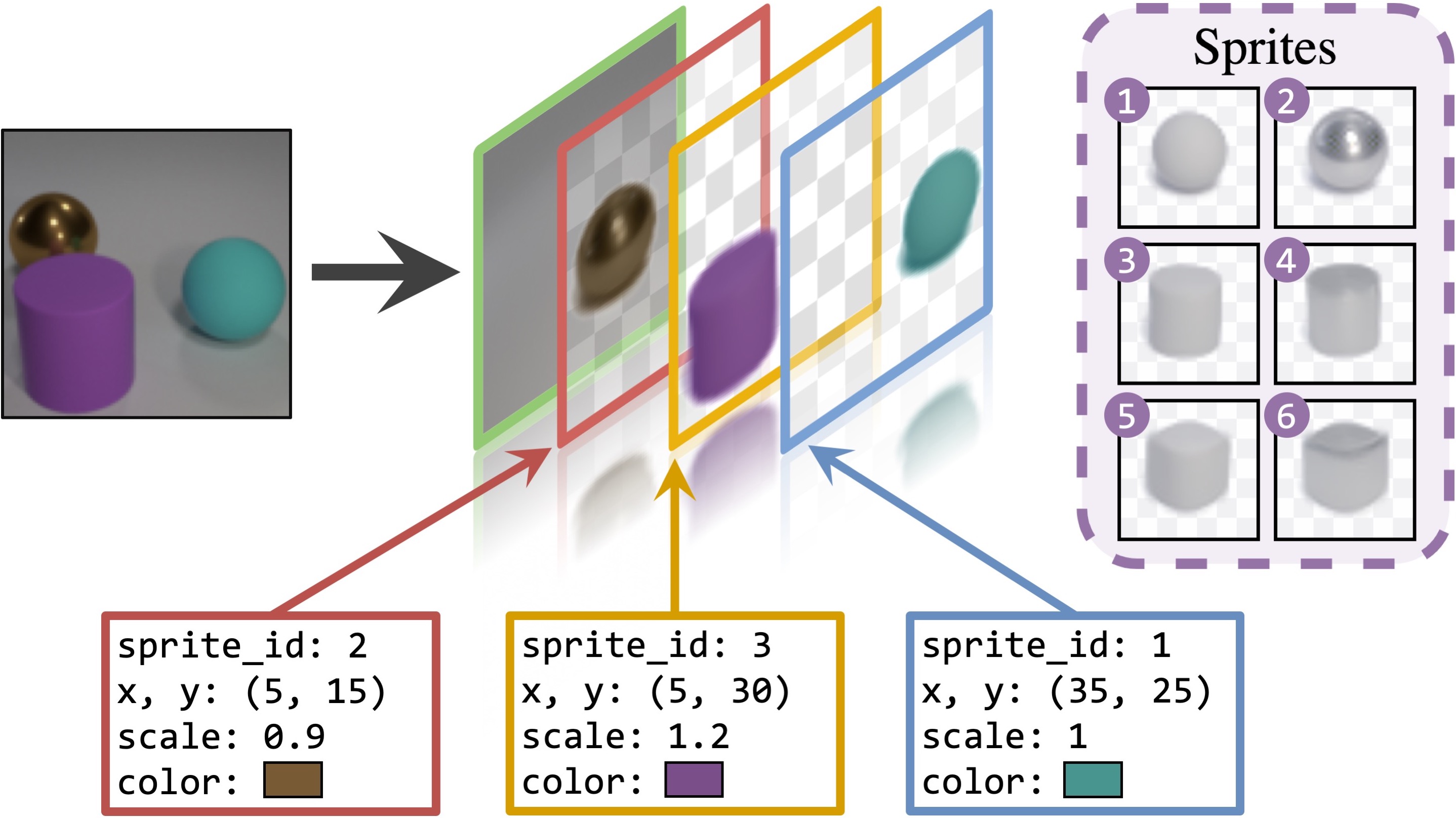
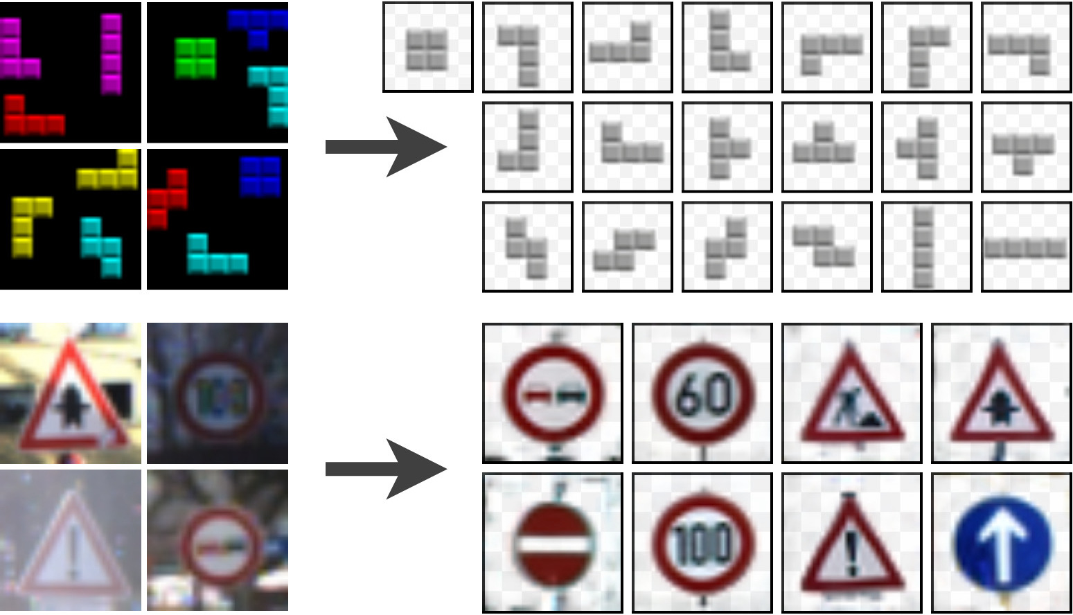
Figure 1: Our approach learns without supervision to decompose images into layers modeled as transformed instances of prototypical objects called sprites. We show an example of decomposition on CLEVR [32] (top) and examples of discovered sprites for Tetrominoes [21] and GTSRB [64] (bottom). Transparency is visualized using light gray checkerboards.

1 Introduction

The aim of this paper is to learn without any supervision a layered decomposition of images, where each layer is a transformed instance of a prototypical object. Such an interpretable and layered model of images could be beneficial for a plethora of applications like object discovery [16, 6], image edition [76, 21], future frame prediction [75], object pose estimation [57] or environment abstraction [1, 47]. Recent works in this direction [6, 21, 49] typically learn layered image decompositions by generating layers with autoencoder networks. In contrast, we explicitly model them as transformations of a set of prototypical images with transparency, which we refer to as sprites. These sprites are mapped onto their instances through geometric and colorimetric transformations resulting in what we call object layers. An image is then assembled from ordered object layers so that each layer occludes previous ones in regions where they overlap.

Our composition model is reminiscent of the classic computer graphics sprite model, popular in console and arcade games from the 1980s. While classical sprites were simply placed at different positions and composited with a background, we revisit the notion in a spirit similar to Jojic and Frey’s work on video modeling [33] by using the term in a more generic sense: our sprites can undergo rich geometric transformations and color changes.

We jointly learn in an unsupervised manner both the sprites and parametric functions predicting their transformations to explain images. This is related to the recent deep transformation-invariant (DTI) method designed for clustering by Monnier et al. [55]. Unlike this work, however, we handle images that involve a variable number of objects with limited spatial supports, explained by different transformations and potentially occluding each other. This makes the problem very challenging because objects cannot be treated independently and the possible number of image compositions is exponential in the number of layers.

We experimentally demonstrate in Section 4.1 that our method is on par with the state of the art on the synthetic datasets commonly used for image decomposition evaluation [21]. Because our approach explicitly models image compositions and object transformations, it also enables us to perform simple and controlled image manipulations on these datasets. More importantly, we demonstrate that our model can be applied to real images (Section 4.2), where it successfully identifies objects and their spatial extent. For example, we report an absolute 5% increase upon the state of the art on the popular SVHN benchmark [56] and good cosegmentation results on the Weizmann Horse database [4]. We also qualitatively show that our model successfully discriminates foreground from background on challenging sets of social network images.

Contributions.

To summarize, we present:

• an unsupervised learning approach that explains images as layered compositions of transformed sprites with a background model;

• strong results on standard synthetic multi-object benchmarks using the usual instance segmentation evaluation, and an additional evaluation on semantic segmentation, which to the best of our knowledge has never been reported by competing methods; and

• results on real images for clustering and cosegmentation, which we believe has never been demonstrated by earlier unsupervised image decomposition models.

Code and data are available on our project webpage.

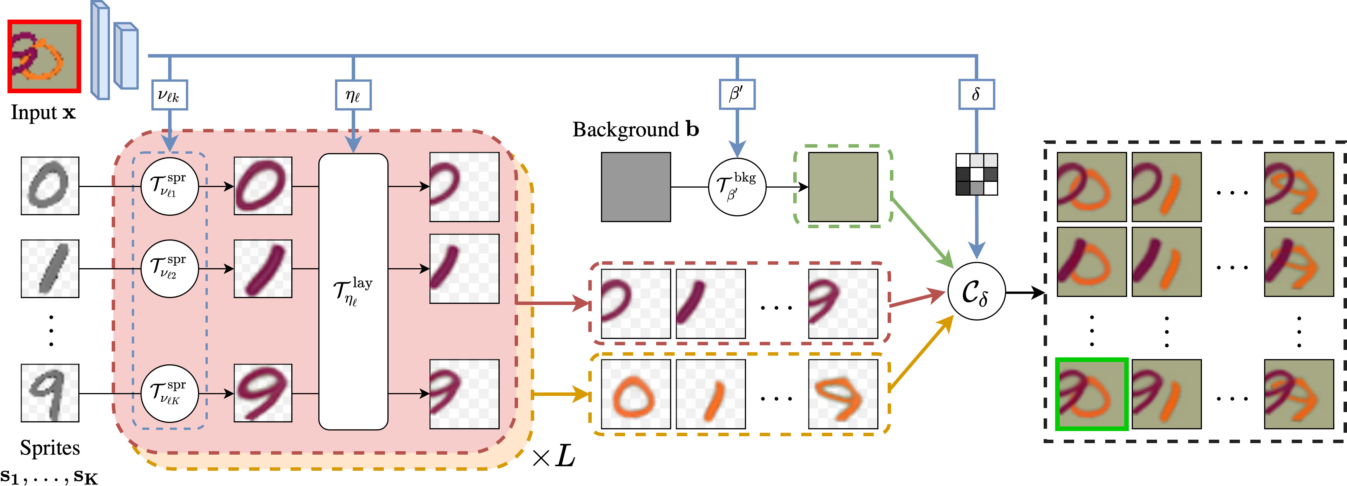
Figure 2: Overview. Given an input image (highlighted in red) we predict for each layer the transformations to apply to the sprites that best reconstruct the input. Transformed sprites and background can be composed into many possible reconstructions given a predicted occlusion matrix $\delta$. We introduce a greedy algorithm to select the best reconstruction (highlighted in green).

2 Related work

Layered image modeling.

The idea of building images by compositing successive layers can already be found in the early work of Matheron [52] introducing the dead leaves models, where an image is assembled as a set of templates partially occluding one another and laid down in layers. Originally meant for material statistics analysis, this work was extended by Lee et al. [43] to a scale-invariant representation of natural images. Jojic and Frey [33] proposed to decompose video sequences into layers undergoing spatial modifications - called flexible sprites - and demonstrated applications to video editing. Leveraging this idea, Winn and Jojic [74] introduced LOCUS, a method for learning an object model from unlabeled images, and evaluated it for foreground segmentation. Recently, approaches [77, 46, 61, 9, 3] have used generative adversarial networks [19] to learn layered image compositions, yet they are limited to foreground/background modeling. While we also model a layered image formation process, we go beyond the simpler settings of image sequences and foreground/background separation by decomposing images into multiple objects, each belonging to different categories and potentially occluding each other.

Image decomposition into objects.

Our work is closely related to a recent trend of works leveraging deep learning to learn object-based image decomposition in an unsupervised setting. A first line of works tackles the problem from a spatial mixture model perspective where latent variables encoding pixel assignment to groups are estimated. Several works from Greff et al. [23, 22, 24] introduce spatial mixtures, model complex pixel dependencies with neural networks and use an iterative refinement to estimate the mixture parameters. MONet [6] jointly learns a recurrent segmentation network and a variational autoencoder (VAE) to predict component mask and appearance. IODINE [21] instead uses iterative variational inference to refine object representations jointly decoded with a spatial broadcast decoder [73] as mixture assignments and components. Combining ideas from MONet and IODINE, GENESIS [15] predicts, with an autoregressive prior, object mask representations used to autoencode masked regions of the input. Leveraging an iterative attention mechanism [68], Slot Attention [49] produces object-centric representations decoded in a fashion similar to IODINE. Other related methods are [67, 72, 78]. Another set of approaches builds upon the work of Eslami et al. introducing AIR [16], a VAE-based model using spatial attention [29] to iteratively specify regions to reconstruct. This notably includes SQAIR [39], SPAIR [13] and the more recent SPACE [47], which in particular incorporates spatial mixtures to model complex backgrounds. To the best of our knowledge, none of these approaches explicitly model object categories, nor demonstrate applicability to real images. In contrast, we represent each type of object by a different prototype and show results on Internet images.

Transformation-invariant clustering.

Identifying object categories in an unsupervised way can be seen as a clustering problem if each image contains a single object. Most recent approaches perform clustering on learned features [25, 31, 38, 66] and do not explicitly model the image. In contrast, transformation-invariant clustering explicitly models transformations to align images before clustering them. Frey and Jojic first introduced this framework [17, 18] by integrating pixel permutation variables within an Expectation-Maximization (EM) [14] procedure. Several works [54, 42, 11, 12] developed a similar idea for continuous parametric transformations in the simpler setting of image alignment, which was later applied again for clustering by [48, 53, 45, 2]. Recently, Monnier et al. [55] generalize these ideas to global alignments and large-scale datasets by leveraging neural networks to predict spatial alignments - implemented as spatial transformers [29] -, color transformations and morphological modifications. Also related to ours, SCAE [38] leverages the idea of capsule [27] to learn affine-aware image features. However, discovered capsules are used as features for clustering and applicability to image decomposition into objects has not been demonstrated.

Cosegmentation and object discovery.

Our method can also be related to traditional approaches for object discovery, where the task is to identify and locate objects without supervision. A first group of methods [62, 60, 7, 63] characterizes images as visual words to leverage methods from topic modeling and localize objects. Another group of methods aims at computing similarities between regions in images and uses clustering models to discover objects. This notably includes [20, 34, 69, 59, 35] for cosegmentation and [58, 10, 70, 44, 71] for object discovery. Although such approaches demonstrate strong results, they typically use hand-crafted features like saliency measures or off-the-shelf object proposal algorithms which are often supervised. More importantly, they do not include an image formation model.

3 Approach

In this section, we first present our image formation model (Sec. 3.1), then describe our unsupervised learning strategy (Sec. 3.2). Figure 2 shows an overview of our approach.

Notations.

We write $a_{1:n}$ the ordered set $\{a_{1},\ldots,a_{n}\}$, $\odot$ pixel-wise multiplication and use bold notations for images. Given $N$ colored images $\mathbf{x}_{1:N}$ of size $H\times W$, we want to learn their decomposition into $L$ object layers defined by the instantiations of $K$ sprites.

3.1 Image formation model

Layered composition process.

Motivated by early works on layered image models [52, 33], we propose to decompose an image into $L$ object layers $\mathbf{o}_{1:L}$ which are overlaid on top of each other. Each object layer $\mathbf{o}_{\ell}$ is a four-channel image of size $H\times W$, three channels correspond to a colored RGB appearance image $\mathbf{o}^{c}_{\ell}$, and the last one $\mathbf{o}^{\alpha}_{\ell}$ is a transparency or alpha channel over $\mathbf{o}^{c}_{\ell}$. Given layers $\mathbf{o}_{1:L}$, we define our image formation process as a recursive composition:

$$\forall\ell>0,\;\mathbf{c}_{\ell}=\mathbf{o}^{\alpha}_{\ell}\odot\mathbf{o}^{c}_{\ell}+(\mathbf{1}-\mathbf{o}^{\alpha}_{\ell})\odot\mathbf{c}_{\ell-1},$$ (1)

where $\mathbf{c}_{0}=\mathbf{0}$, and the final result of the composition is $\mathbf{c}_{L}$. Note that this process explicitly models occlusion: the first layer corresponds to the farthest object from the camera, and layer $L$ is the closest, occluding all the others. In particular, we model background by using a first layer with $\mathbf{o}^{\alpha}_{1}=1$.

Unfolding the recursive process in Eq. (1), the layered composition process can be rewritten in the compact form:

$${\mathcal{C}}_{\delta}(\mathbf{o}_{1},\ldots,\mathbf{o}_{L})=\sum_{\ell=1}^{L}\Big{(}\prod_{j=1}^{L}(\mathbf{1}-\delta_{j\ell}\mathbf{o}^{\alpha}_{j})\Big{)}\odot\mathbf{o}^{\alpha}_{\ell}\odot\mathbf{o}^{c}_{\ell},$$ (2)

where $\delta_{j\ell}=\mathbbm{1}_{[j>\ell]}$ is the indicator function of $j>\ell$. $\delta$ is a $L\times L$ binary matrix we call occlusion matrix: for given indices $j$ and $\ell$, $\delta_{j\ell}=1$ if layer $j$ occludes layer $\ell$, and $\delta_{j\ell}=0$ otherwise. This gives Eq. (2) a clear interpretation: each layer appearance $\mathbf{o}^{c}_{\ell}$ is masked by its own transparency channel $\mathbf{o}^{\alpha}_{\ell}$ and other layers $j$ occluding it, i.e. for which $\delta_{j\ell}=1$. Note that we explicitly introduce the dependency on $\delta$ in the composition process ${\mathcal{C}}_{\delta}$ because we will later predict it, which intuitively corresponds to a layer reordering.

Sprite modeling.

We model each layer as an explicit transformation of one of $K$ learnable sprites $\mathbf{s}_{1:K}$, which can be seen as prototypes representing the object categories. Each sprite $\mathbf{s}_{k}$ is a learnable four-channel image of arbitrary size, an RGB appearance image $\mathbf{s}^{c}_{k}$ and a transparency channel $\mathbf{s}^{\alpha}_{k}$. To handle variable number of objects, we model object absence with an empty sprite $\mathbf{s}_{0}=\mathbf{0}$ added to the $K$ sprite candidates and penalize the use of non-empty sprites during learning (see Sec. 3.2). Such modeling assumes we know an upper bound of the maximal number of objects, which is rather standard in such a setting [6, 21, 49].

Inspired by the recent deep transformation-invariant (DTI) framework designed for clustering [55], we assume that we have access to a family of differentiable transformations ${\mathcal{T}}_{\beta}$ parametrized by $\beta$ - e.g. an affine transformation with $\beta$ in ${\mathbb{R}}^{6}$ implemented with a spatial transformer [29] - and we model each layer as the result of the transformation ${\mathcal{T}}_{\beta}$ applied to one of the $K$ sprites. We define two sets of transformations for a given layer $\ell$: (i) ${\mathcal{T}}^{\,\textrm{\scriptsize lay}}_{\eta_{\ell}}$ the transformations parametrized by $\eta_{\ell}$ and shared for all sprites in that layer, and (ii) ${\mathcal{T}}^{\,\textrm{\scriptsize spr}}_{\nu_{\ell k}}$ the transformations specific to each sprite and parametrized by $\nu_{\ell k}$. More formally, for given layer $\ell$ and sprite $k$ we write:

$${\mathcal{T}}_{\beta_{\ell k}}(\mathbf{s}_{k})={\mathcal{T}}^{\,\textrm{\scriptsize lay}}_{\eta_{\ell}}\circ{\mathcal{T}}^{\,\textrm{\scriptsize spr}}_{\nu_{\ell k}}(\mathbf{s}_{k}),$$ (3)

where $\beta_{\ell k}=(\eta_{\ell},\nu_{\ell k})$ and ${\mathcal{T}}_{(\eta_{\ell},\nu_{\ell k})}={\mathcal{T}}^{\,\textrm{\scriptsize lay}}_{\eta_{\ell}}\circ{\mathcal{T}}^{\,\textrm{\scriptsize spr}}_{\nu_{\ell k}}$.

Although it could be included in ${\mathcal{T}}^{\,\textrm{\scriptsize spr}}_{\nu_{\ell k}}$, we separate ${\mathcal{T}}^{\,\textrm{\scriptsize lay}}_{\eta_{\ell}}$ to constrain transformations and avoid bad local minima. For example, we use it to model a coarse spatial positioning so that all sprites in a layer attend to the same object in the image. On the contrary, we use ${\mathcal{T}}^{\,\textrm{\scriptsize spr}}_{\nu_{\ell k}}$ to model sprite specific deformations, such as local elastic deformations.

When modeling background, we consider a distinct set of $K^{\prime}$ background prototypes $\mathbf{b}_{1:K^{\prime}}$, without transparency, and different families of transformations ${\mathcal{T}}^{\,\textrm{\scriptsize bkg}}_{\beta^{\prime}}$. For simplicity, we write the equations for the case without background and omit sprite-specific transformations in the rest of the paper, writing ${\mathcal{T}}_{\beta_{\ell}}(\mathbf{s}_{k})$ instead of ${\mathcal{T}}_{\beta_{\ell k}}(\mathbf{s}_{k})$.

To summarize, our image formation model is defined by the occlusion matrix $\delta$, the per-layer sprite selection $(k_{1},\ldots,k_{L})$, the corresponding transformation parameters $(\beta_{1},\ldots,\beta_{L})$, and outputs an image $\mathbf{x}$ such that:

$$\mathbf{x}={\mathcal{C}}_{\delta}\Big{(}{\mathcal{T}}_{\beta_{1}}(\mathbf{s}_{k_{1}}),\ldots,{\mathcal{T}}_{\beta_{L}}(\mathbf{s}_{k_{L}})\Big{)}.$$ (4)

We illustrate our image formation model in Figure 1 and provide a detailed example in Figure 2.

3.2 Learning

We learn our image model without any supervision by minimizing the objective function:

$${\mathcal{L}}(\mathbf{s}_{1:K},\phi_{1:L},\psi)=\sum_{i=1}^{N}\;\min_{k_{1},\ldots,k_{L}}\Big{(}\lambda\sum_{j=1}^{L}\mathbbm{1}_{[k_{j}\neq 0]}+\\ \Big{\|}\mathbf{x}_{i}-{\mathcal{C}}_{\psi(\mathbf{x}_{i})}\scaleto{\Big{(}{\mathcal{T}}_{{\phi_{1}}(\mathbf{x}_{i})}(\mathbf{s}_{k_{1}}),\ldots,{\mathcal{T}}_{{\phi_{L}}(\mathbf{x}_{i})}(\mathbf{s}_{k_{L}})\Big{)}}{17pt}\Big{\|}^{2}_{2}\Big{)},$$ (5)

where $\mathbf{s}_{1:K}$ are the sprites, $\phi_{1:L}$ and $\psi$ are neural networks predicting the transformation parameters and occlusion matrix for a given image $\mathbf{x}_{i}$, $\lambda$ is a scalar hyper-parameter and $\mathbbm{1}_{[k_{j}\neq 0]}$ is the indicator function of $k_{j}\neq 0$. The first sum is over all images in the database, the minimum corresponds to the selection of the sprite used for each layer and the second sum counts the number of non-empty sprites. If $\lambda>0$, this loss encourages reconstructions using the minimal number of non-empty sprites. In practice, we use $\lambda=10^{-4}$.

Note the similarity between our loss and the gradient-based adaptation [5] of the K-means algorithm [50] where the squared Euclidean distance to the closest prototype is minimized, as well as with its transformation-invariant version [55] including neural networks modeling transformations. In addition to the layered composition model described in the previous section, the main two differences with our model are the joint optimization over $L$ sprite selections and the occlusion modeling that we discuss next.

Sprites selection.

Because the minimum in Eq. (5) is taken over the $(K+1)^{L}$ possible selections leading to as many reconstructions, an exhaustive search over all combinations quickly becomes impossible when dealing with many objects and layers. Thus, we propose an iterative greedy algorithm to estimate the minimum, described in Algorithm 1 and used when $L>2$. While the solution it provides is of course not guaranteed to be optimal, we found it performs well in practice. At each iteration, we proceed layer by layer and iteratively select for each layer the sprite $k_{\ell}$ minimizing the loss, keeping all other object layers fixed. This reduces the number of reconstructions to perform to $T\times(K+1)\times L$. In practice, we have observed that convergence is reached after 1 iteration for Tetrominoes and 2-3 iterations for Multi-dSprites and CLEVR6, so we have respectively used $T=1$ and $T=3$ in these experiments. We experimentally show in our ablation study presented in Sec. 4.1 that this greedy approach yields performances comparable to an exhaustive search when modeling small numbers of layers and sprites.

Input: image $\mathbf{x}$, occlusion $\delta$, $(K+1)\times L$ object layers candidates ${\mathcal{T}}_{{\phi_{\ell}}(\mathbf{x})}(\mathbf{s}_{k})$, steps $T$

Output: sprite indices $(k_{1},\ldots,k_{L})$

Initialization: $\forall\ell\in\{1,\ldots,L\},\;k_{\ell}\leftarrow{0},\mathbf{o}_{\ell}\leftarrow\mathbf{0}$

1 for $t=1,\ldots,T$ do # iterations

2      for $\ell=1,\ldots,L$ do # loop on layers

3            $k_{\ell}\leftarrow\min_{k}\,\Big{[}\lambda\mathbbm{1}_{[k\neq 0]}\;+$

4                       $\|\mathbf{x}-{\mathcal{C}}_{\delta}(\mathbf{o}_{1:\ell-1},\,{\mathcal{T}}_{{\phi_{\ell}}(\mathbf{x})}(\mathbf{s}_{k}),\,\mathbf{o}_{\ell+1:L})\|^{2}_{2}\Big{]}$

5             $\mathbf{o}_{\ell}\leftarrow{\mathcal{T}}_{{\phi_{\ell}}(\mathbf{x})}(\mathbf{s}_{k_{\ell}})$

6       end for

7      

8 end for

return $k_{1},\ldots,k_{L}$

Algorithm 1 Greedy sprite selection.

Occlusion modeling.

Occlusion is modeled explicitly in our composition process defined in Eq. (2) since $\mathbf{o}_{1},\ldots,\mathbf{o}_{L}$ are ranked by depth. However, we experimentally observed that layers learn to specialize to different regions in the image. This seems to correspond to a local minimum of the loss function, and the model does not manage to reorder the layers to predict the correct occlusion. Therefore, we relax the model and predict an occlusion matrix $\delta=\psi(\mathbf{x})\in[0,1]^{L\times L}$ instead of keeping it fixed. More precisely, for each image $\mathbf{x}$ we predict $\frac{1}{2}L(L-1)$ values using a neural network followed by a sigmoid function. These values are then reshaped to a lower triangular $L\times L$ matrix with zero diagonal, and the upper part is computed by symmetry such that: $\forall i<j,\,\delta_{ij}=1-\delta_{ji}$. While such predicted occlusion matrix is not binary and does not directly translate into a layer reordering, it still allows us to compute a composite image using Eq. (2) and the masks associated to each object. Note that such a matrix could model more complex occlusion relationships such as non-transitive ones. At inference, we simply replace $\delta_{ij}$ by $\delta_{ij}>0.5$ to obtain binary occlusion relationships. We also tried computing the closest matrix corresponding to a true layer reordering and obtained similar results. Note that when we use a background model, its occlusion relationships are fixed, i.e. $\forall j>1,\delta_{j1}=1$.

Training details.

Two elements of our training strategy are crucial to the success of learning. First, following [55] we adopt a curriculum learning of the transformations, starting by the simplest ones. Second, inspired by Tieleman [65] and SCAE [38], we inject uniform noise in the masks in such a way that masks are encouraged to be binary (see supplementary for details). This allows us to resolve the ambiguity that would otherwise exist between the color and alpha channels and obtain clear masks. We provide additional details about networks’ architecture, computational cost, transformations used and implementation in the supplementary material.

4 Experiments

Assessing the quality of an object-based image decomposition model is ambiguous and difficult, and downstream applications on synthetic multi-object benchmarks such as [36] are typically used as evaluations. Thus, recent approaches (e.g. [6, 21, 15, 49]) first evaluate their ability to infer spatial arrangements of objects through quantitative performances for object instance discovery. The knowledge of the learned concept of object is then evaluated qualitatively through convincing object-centric image manipulation [6, 21], occluded region reconstructions [6, 49] or realistic generative sampling [15]. None of these approaches explicitly model categories for objects and, to the best of our knowledge, their applicability is limited to synthetic imagery only.

In this section, we first evaluate and analyse our model on the standard multi-object synthetic benchmarks (Sec. 4.1). Then, we demonstrate that our approach can be applied to real images (Sec. 4.2). We use the 2-layer version of our model to perform clustering (4.2.1), cosegmentation (4.2.2), as well as qualitative object discovery from unfiltered web image collections (4.2.3).

4.1 Multi-object synthetic benchmarks

Datasets and evaluation.

Tetrominoes [21] is a 60k dataset generated by placing three Tetrominoes without overlap in a $35\times 35$ image. There is a total of 19 different Tetrominoes (counting discrete rotations). Multi-dSprites [36] contains 60k images of size $64\times 64$ with 2 to 5 objects sampled from a set of 3 different shapes: ellipse, heart, square. CLEVR6 [32, 21] contains 34,963 synthetically generated images of size $128\times 128$. Each image is composed of a variable number of objects (from 3 to 6), each sampled from a set of 6 categories - 3 different shapes (sphere, cylinder, cube) and 2 materials (rubber or metal) - and randomly rendered. We thus train our method using one sprite per object category and as many layers as the maximum number of objects per image, with a background layer when necessary. Following standard practices [21, 49], we evaluate object instance segmentation on 320 images by averaging over all images the Adjusted Ranked Index (ARI) computed using ground-truth foreground pixels only (ARI-FG in our tables). Note that because background pixels are filtered, ARI-FG strongly favors methods like [21, 49] which oversegment objects or do not discriminate foreground from background. To limit the penalization of our model which explicitly models background, we reassign predicted background pixels to the closest object layers before computing this metric. However, we argue that foreground/background separation is crucial for any downstream applications and also advocate the use of a true ARI metric computed on all pixels (including background) which we include in our results. In addition, we think that the knowledge of object category should be evaluated and include quantitative results for unsupervised semantic segmentation in the supplementary material.

Results.

Our results are compared quantitatively to state-of-the-art approaches in Table 1. On Multi-dSprites, an outlier run out of 5 was automatically filtered based on its high reconstruction loss compared to the others. Our method obtains results on par with the best competing methods across all benchmarks. While our approach is more successful on benchmarks depicting 2D scenes, it still provides good results on CLEVR6 where images include 3D effects. We provide our results using the real ARI metric which we believe to be more interesting as it is not biased towards oversegmenting methods. While this measure is not reported by competing methods, a CLEVR6 decomposition example shown in official IODINE implementation gives a perfect 100% ARI-FG score but reaches 20% in terms of ARI.

Table 1: Multi-object instance discovery. Following standard practices, we report ARI-FG (ARI on foreground pixels only) averaged over 5 runs. We also report our results with the real ARI, a metric we advocate for future comparisons. We mark results ($\vartriangle$) where one outlier run is filtered out.

Method	Metric	Tetrominoes	Multi-dSprites	CLEVR6
MONet [6]	ARI-FG	-	90.4 $\pm$ 0.8	96.2 $\pm$ 0.6
IODINE [21]	ARI-FG	99.2 $\pm$ 0.4	76.7 $\pm$ 5.6	98.8 $\pm$ 0.0
Slot Att. [49]	ARI-FG	99.5${}^{\vartriangle}\pm$ 0.2	91.3 $\pm$ 0.3	98.8 $\pm$ 0.3
Ours	ARI-FG	99.6 $\pm$ 0.2	92.5${}^{\vartriangle}\pm$ 0.3	$97.2\pm 0.2$
Ours	ARI	99.8 $\pm$ 0.1	95.1${}^{\vartriangle}\pm$ 0.1	90.7 $\pm$ 0.1

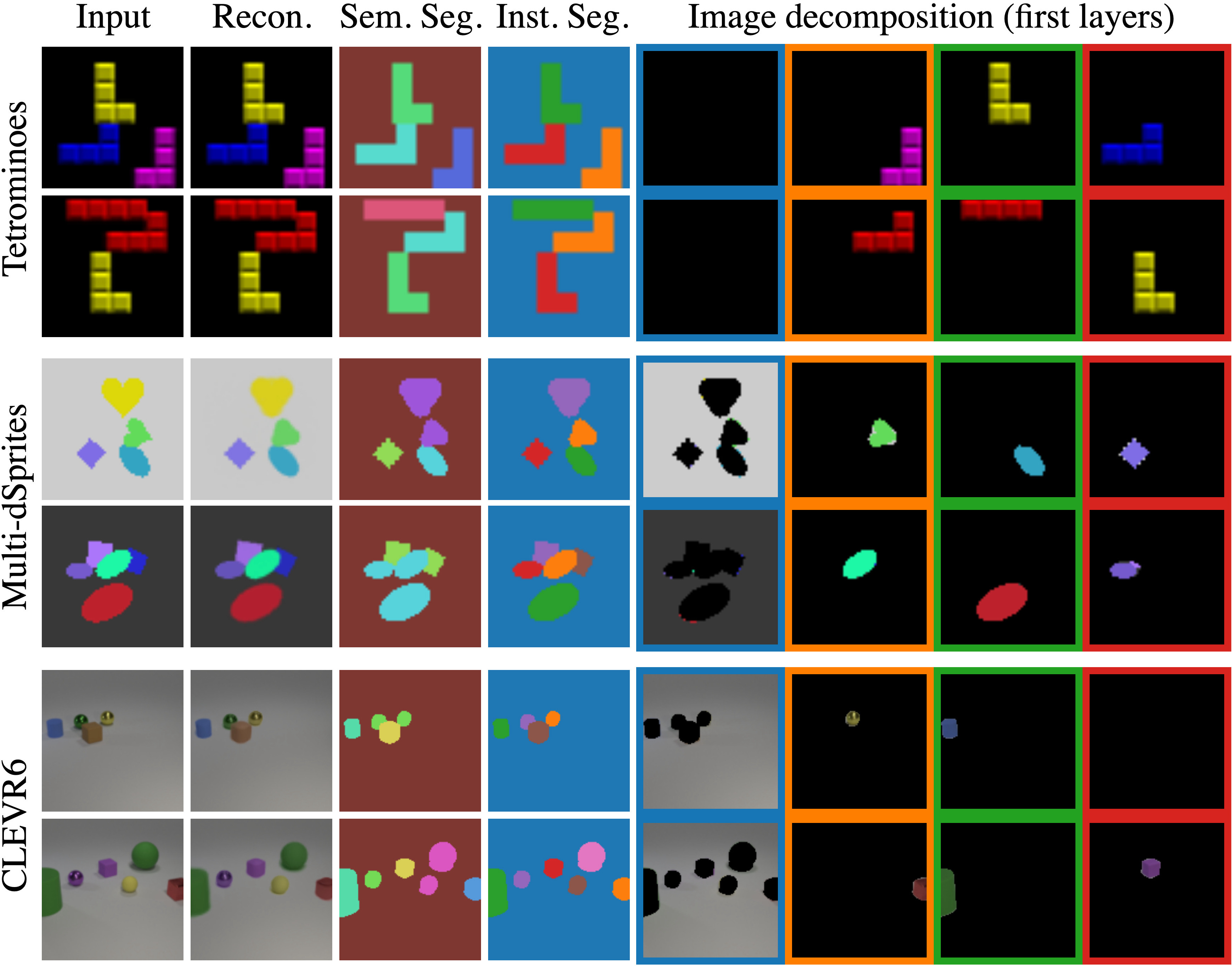
Figure 3: Multi-object discovery. From left to right, we show inputs, reconstructions, semantic (each color corresponds to a different sprite) and instance segmentations, and first decomposition layers colored w.r.t. their instance mask.

Compared to all competing methods, our approach explicitly models categories for objects. In particular, it is able to learn prototypical images that can be associated to each object category. The sprites discovered from CLEVR6 and Tetrominoes are shown in Fig. 1. Note how learned sprites on Tetrominoes are sharp and how we can identify material in CLEVR6 by learning two different sprites for each shape.

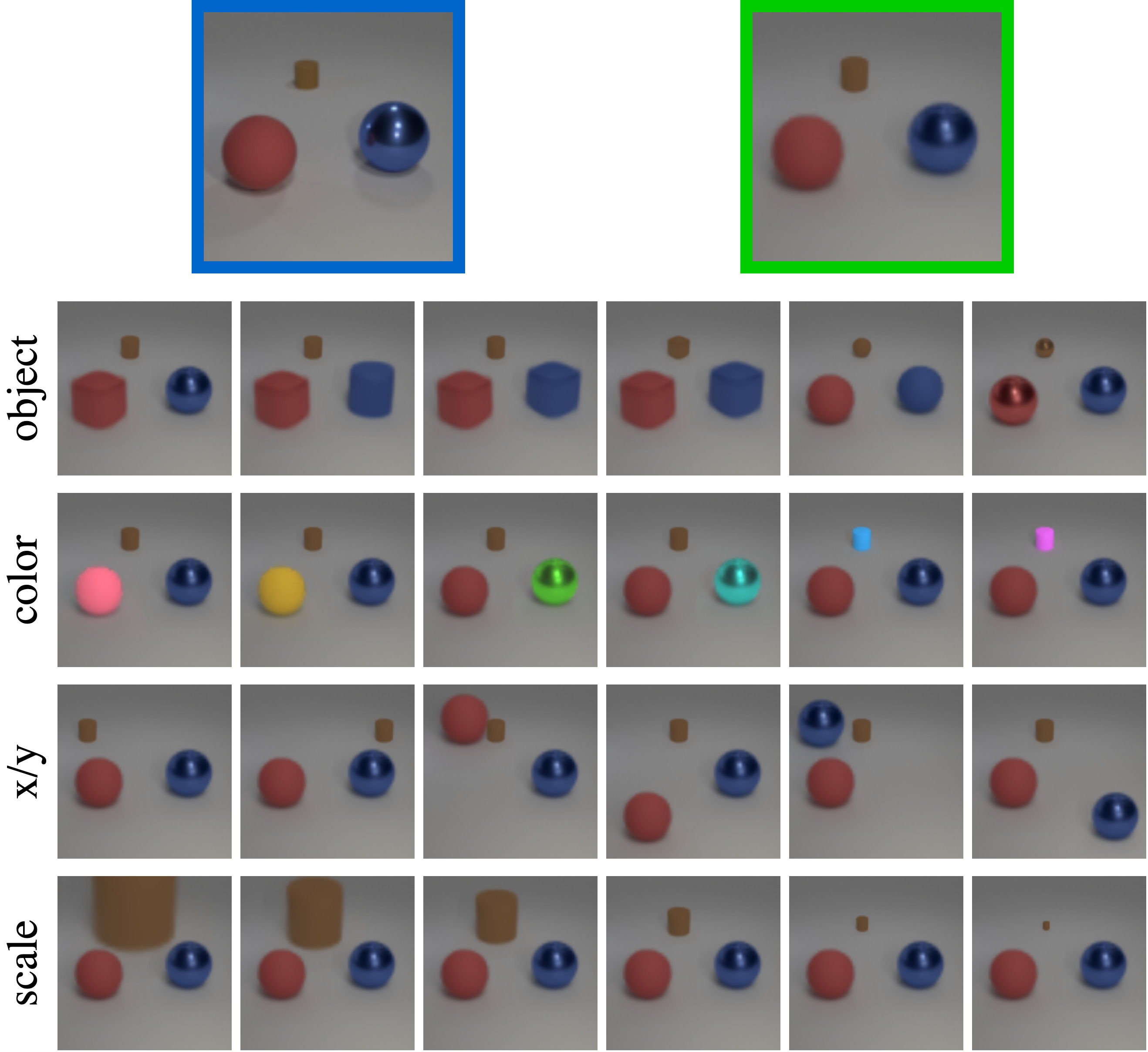
Figure 4: Object-centric image manipulation. Given a query image (top left) from CLEVR6 [32], we show the closest reconstruction (top right) and several image manipulations (next four rows). From top to bottom, we respectively use different sprites, change the objects color, vary their positions and modify the scale.

In Fig. 3, we show some qualitative results obtained on the three benchmarks. Given sample images, we show from left to right the final reconstruction, semantic segmentation (evaluated quantitatively in the supplementary material) where each color corresponds to a different sprite, instance segmentation, and the first four layers of the image decomposition. Note how we manage to successfully predict occlusions, model variable number of objects, separate the different instances, as well as identify the object categories and their spatial extents. More random decomposition results are shown in the supplementary and on our webpage.

Compared to other approaches which typically need a form of supervision to interpret learned representations as object visual variations, our method has the advantage to give a direct access to the object instance parameters, enabling us to directly manipulate them in images. In Fig. 4, we show different object-centric image manipulations such as objects swapping as well as color, position and scale variations. Note that we are also able to render out of distribution instances, like the pink sphere or the gigantic cylinder.

Table 2: Ablation study. Results are averaged over 5 runs.

Dataset	Model	ARI-FG	ARI
Multi-dSprites2	Full	95.5 $\pm$ 2.1	95.2 $\pm$ 1.9
	w/o greedy algo.	94.4 $\pm$ 2.7	95.9 $\pm$ 0.3
Multi-dSprites	Full	91.5 $\pm$ 2.2	95.0 $\pm$ 0.3
	w/o occ. prediction	85.7 $\pm$ 2.2	94.2 $\pm$ 0.2
Tetrominoes	Full	99.6 $\pm$ 0.2	99.8 $\pm$ 0.1
	w/o shared transfo.	95.3 $\pm$ 3.7	82.6 $\pm$ 12.2

Ablation study.

We analyze the main components of our model in Table 2. For computational reasons, we evaluate our greedy algorithm on Multi-dSprites2 - the subset of Multi-dSprites containing only 2 objects - and show comparable performances to an exhaustive search over all combinations. Occlusion prediction is evaluated on Multi-dSprites which contains many occlusions. Because our model with fixed occlusion does not manage to reorder the layers, performances are significantly better when occlusion is learned. Finally, we compare results obtained on Tetrominoes when modeling sprite-specific transformations only, without shared ones, and show a clear gap between the two settings. We provide analyses on the effects of $K$ and $\lambda$ in the supplementary.

Limitations.

Our optimization model can be stuck in local minima. A typical failure mode on Multi-dSprites can be seen in the reconstructions in Fig. 3 where a triangular shape is learned instead of the heart. This sprite can be aligned to a target heart shape using three different equivalent rotations, and our model does not manage to converge to a consistent one. This problem could be overcome by either modeling more sprites, manually computing reconstructions with different discrete rotations, or guiding transformation predictions with supervised sprite transformations.

4.2 Real image benchmarks

4.2.1 Clustering

Datasets.

We evaluate our model on two real image clustering datasets using 2 layers, one for the background and one for the foreground object. SVHN [56] is a standard clustering dataset composed of digits extracted from house numbers cropped from Google Street View images. Following standard practices [28, 38, 55], we evaluate on the labeled subset (99,289 images), but also use 530k unlabeled extra samples for training. We also report results on traffic sign images using a balanced subset of the GTSRB dataset [64] which we call GTSRB-8. We selected classes with 1000 to 1500 instances in the training split, yielding 8 classes and 10,650 images which we resize to $28\times 28$.

Results.

We compare our model to state-of-the-art methods in Table 3 using global clustering accuracy, where the cluster-to-class mapping is computed using the Hungarian algorithm [40]. We train our 2-layer model with as many sprites as classes and a single background prototype. On both benchmarks, our approach provides competitive results. In particular, we improve state of the art on the standard SVHN benchmark by an absolute 5% increase.

Similar to DTI-Clustering, our method performs clustering in pixel-space exclusively and has the advantage of providing interpretable results. Figure 5 shows learned sprites on the GTSRB-8 and SVHN datasets and compares them to prototypes learned with DTI-Clustering. Note in particular the sharpness of the discovered GTSRB-8 sprites.

Table 3: Clustering comparisons. We report average clustering accuracy. We mark methods we ran ourselves with official implementations ($\star$), use data augmentation ($\triangledown$) or ad-hoc representations ($\dagger$ for GIST, $\ddagger$ for Sobel filters).

Method	Runs	GTSRB-8	SVHN
Clustering on learned features
ADC [25]	20	-	38.6▽
SCAE [38]	5	-	55.3‡
IMSAT [28]	12	26.9▽⋆	57.3▽†
SCAN [66]	5	90.4▽⋆	54.2▽⋆
Clustering on pixel values
DTI-Clustering [55]	10	54.3⋆	57.4
Ours	10	89.4	63.1

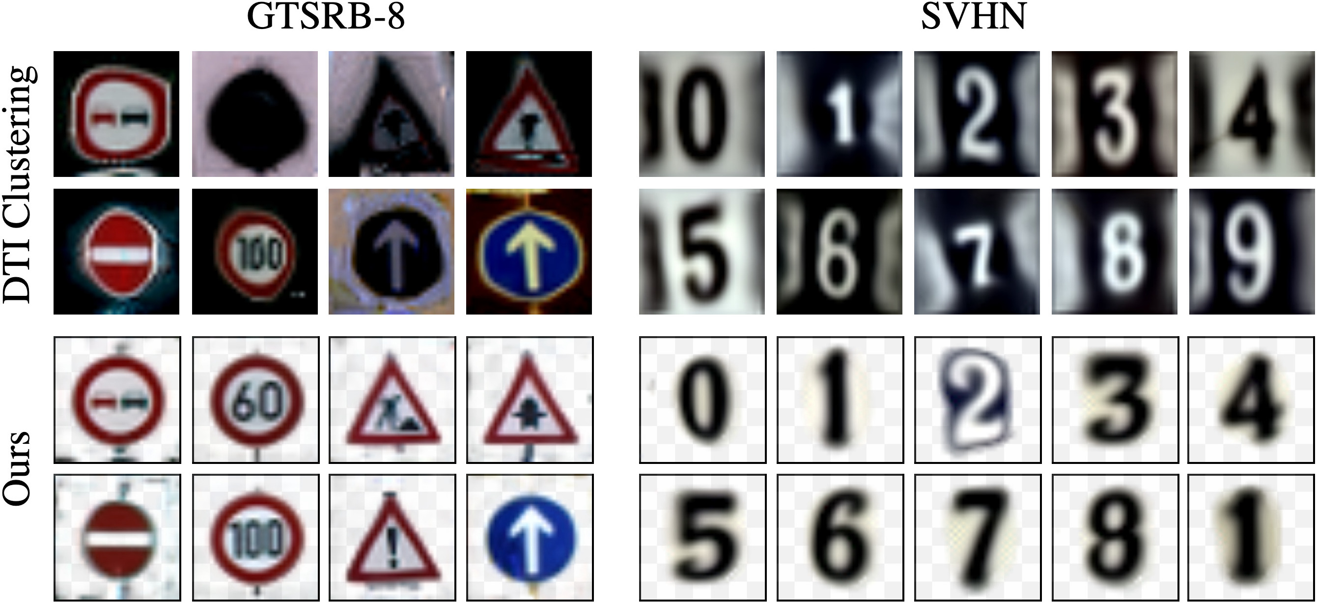
Figure 5: Qualitative clustering results. We compare prototypes learned using DTI-Clustering and our discovered sprites on GTSRB-8 (left) and SVHN (right).

4.2.2 Cosegmentation

Dataset.

We use the Weizmann Horse database [4] to evaluate quantitatively the quality of our masks. It is composed of 327 side-view horse images resized to $128\times 128$. Although relatively simple compared to more recent cosegmentation datasets, it presents significant challenges compared to previous synthetic benchmarks because of the diversity of both horses and backgrounds. The dataset was mainly used by classical (non-deep) methods which were trained and evaluated on 30 images for computational reasons while we train and evaluate on the full set.

Results.

We compare our 2-layer approach with a single sprite to classical cosegmentation methods in Table 4 and report segmentation accuracy - mean % of pixels correctly classified as foreground or background - averaged over 5 runs. Our results compare favorably to these classical approaches. Although more recent approaches could outperform our method on this dataset, we argue that obtaining performances on par with such competing methods is already a strong result for our layered image decomposition model.

We present in Fig. 6 some visual results of our approach. First, the discovered sprite clearly depicts a horse shape and its masks is sharp and accurate. Learning such an interpretable sprite from this real images collection is already interesting and validates that our sprite-based modeling generalizes to real images. Second, although the transformations modeled are quite simple (a combination of color and spatial transformations), we demonstrate good reconstructions and decompositions, yielding accurate foreground extractions.

Table 4: Weizmann Horse cosegmentation comparisons.

Method	[59]	[34]	[41]	[8]	[79]	Ours
Accuracy (%)	74.9	80.1	84.6	86.4	87.6	87.9

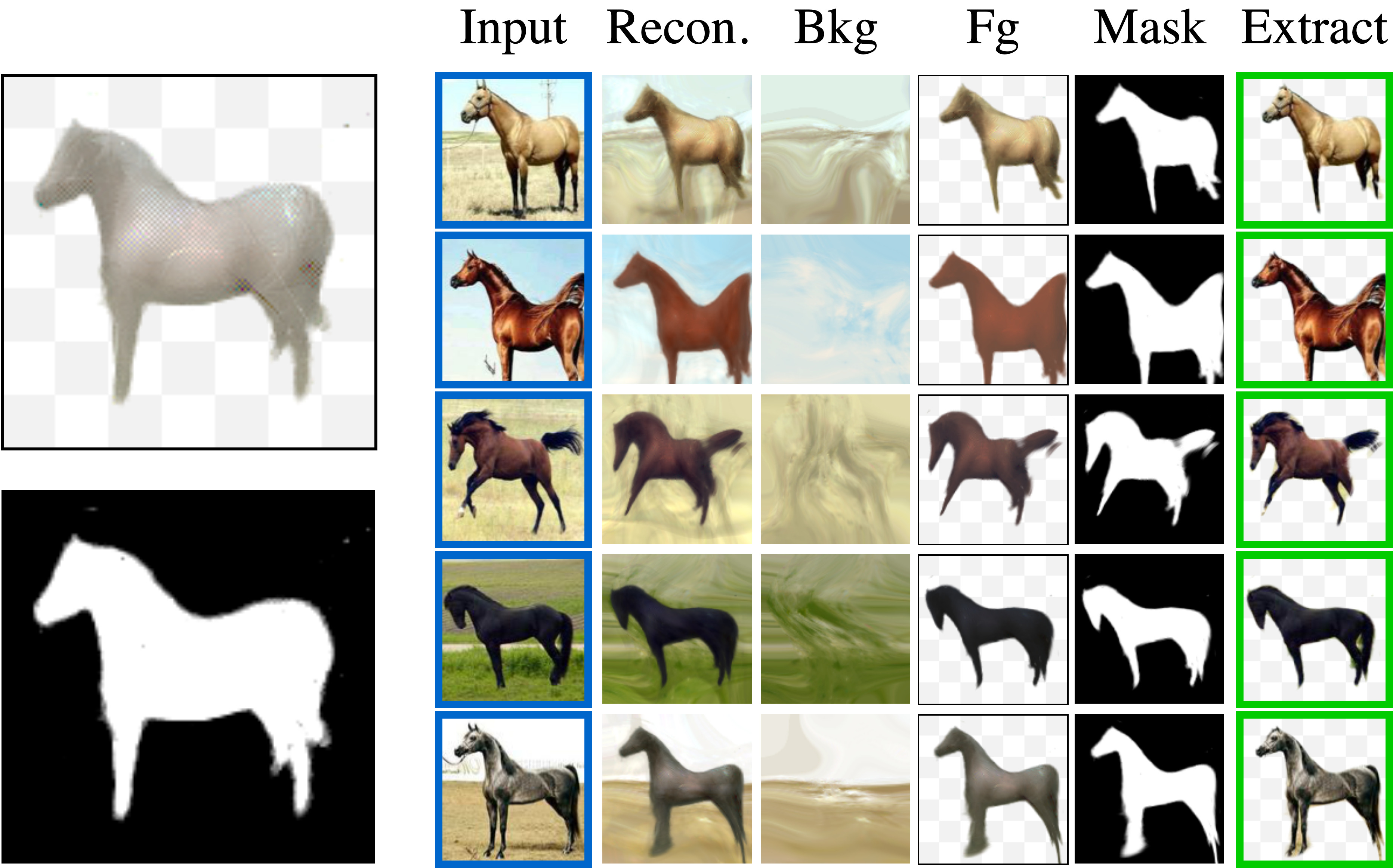
Figure 6: Qualitative cosegmentation results. Sprite and mask (left) learned from Weizmann Horse [4] and some result examples (right) giving for each input, its reconstruction, the layered composition and extracted foreground.

4.2.3 Unfiltered web image collections

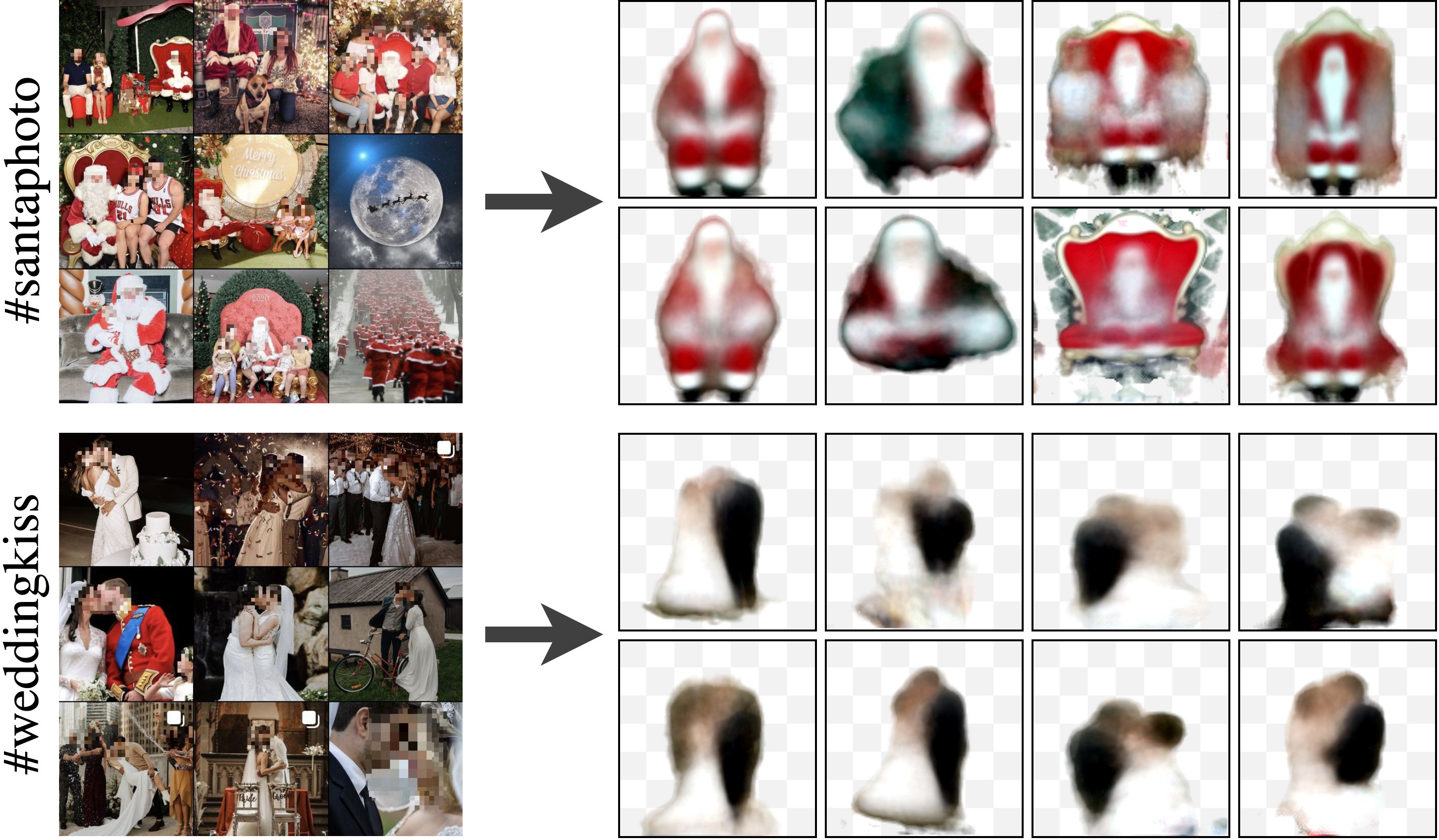
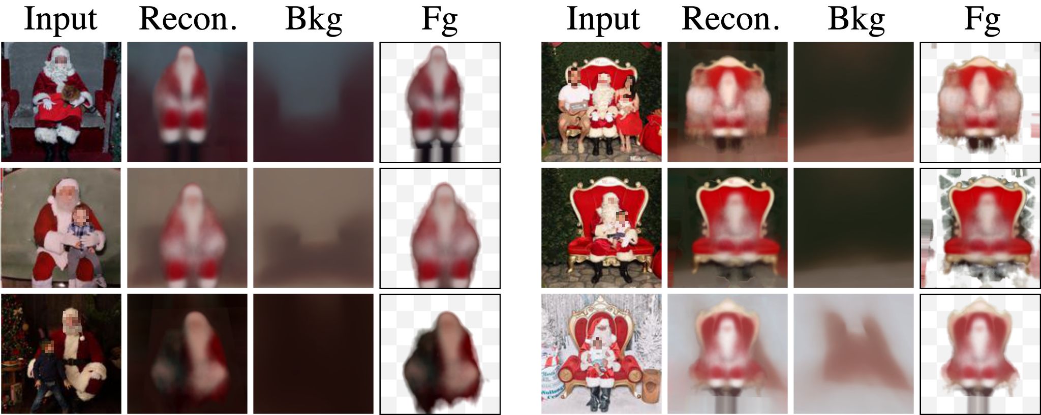
Figure 7: Web image results. We show the 8 best qualitative sprites among 40 discovered from Instagram collections (top) as well as decomposition results for samples represented by one of the sprites shown for #santaphoto (bottom).

We demonstrate our approach’s robustness by visualizing sprites discovered from web image collections. We use the same Instagram collections introduced in [55], where each collection is associated to a specific hashtag and contains around 15k images resized and center cropped to $128\times 128$. We apply our model with 40 sprites and a background.

Figure 7 shows the 8 best qualitative sprites discovered from Instagram collections associated to #santaphoto and #weddingkiss. Even in this case where images are mostly noise, our approach manages to discover meaningful sprites and segmentations with clear visual variations. For example, we can distinguish standing santas from seating ones, as well as the ones alone or surrounded by children. We additionally show examples of reconstructions and image compositions for some of the 8 sprites shown for #santaphoto.

5 Conclusion

We have introduced a new unsupervised model which jointly learns sprites, transformations and occlusions to decompose images into object layers. Beyond standard multi-object synthetic benchmarks, we have demonstrated that our model leads to actual improvements for real image clustering with a 5% boost over the state of the art on SVHN and can provide good segmentation results. We even show it is robust enough to provide meaningful results on unfiltered web image collections. Although our object modeling involves unique prototypical images and small sets of transformations limiting their instances diversity, we argue that accounting for such diversity while maintaining a category-based decomposition model is extremely challenging, and our approach is the first to explore this direction as far as we know.

Supplementary Material for
Unsupervised Layered Image Decomposition into Object Prototypes

In this supplementary document, we provide quantitative semantic segmentation results (Section A), analyses of the model (Section B), training details (Section C) and additional qualitative results (Section D).

Appendix A Quantitative semantic segmentation results

We provide a quantitative evaluation of our approach in an unsupervised semantic segmentation setting. We do not compare to state-of-the-art approaches as none of them explicitly model nor output categories for objects. We argue that modeling categories for discovered objects is crucial to analyse and understand scenes, and thus advocate such quantitative semantic evaluation to assess the quality of any object-based image decomposition algorithm.

Evaluation.

Motivated by standard practices from supervised semantic segmentation and clustering benchmarks, we evaluate our unsupervised object semantic segmentation results by computing the mean accuracy (mACC) and the mean intersection-over-union (mIoU) across all classes (including background). We first compute the global confusion matrix on the same 320 images used for object instance segmentation evaluation. Then, we reorder the matrix with a cluster-to-class mapping computed using the Hungarian algorithm [40]. Finally, we average accuracy and intersection-over-union over all classes, including background, respectively yielding mACC and mIoU.

Results.

Our performances averaged over 5 runs are reported in Table 5. Similar to our results for object instance segmentation, we filter an outlier run out of 5 for Multi-dSprites based on its high reconstruction loss compared to other runs ($1.93\times 10^{-3}$ against $\{1.51,1.49,1.52,1.57\}\times 10^{-3}$). For Tetrominoes and Multi-dSprites, our method obtains strong results thus emphasizing that our 2D prototype-based modeling is well suited for such 2D scene benchmarks. On the contrary for CLEVR6, there is still room for improvements. Although we can distinguish the 6 different categories from discovered sprites, such performances suggest that our model struggles to accurately transform the sprites to match the target object instances. This is expected since we do not explicitly account for neither 3D, lighting nor material effects in our modeling.

Table 5: Multi-object semantic discovery. We report our mACC and mIoU performances averaged over 5 runs with stddev. $K$ refers to the number of classes (including background) and we mark results ($\vartriangle$) where one outlier run was automatically filtered out.

Dataset	$K$	mACC	mIoU
Tetrominoes [21]	20	99.5 $\pm$ 0.2	99.1 $\pm$ 0.4
Multi-dSprites [36]	4	91.3${}^{\vartriangle}\pm$ 0.9	84.0${}^{\vartriangle}\pm$ 1.4
CLEVR6 [32, 21]	7	73.9 $\pm$ 2.1	56.3 $\pm$ 2.9

Appendix B Model analysis

B.1 Effect of $K$

Similar to standard clustering methods, our results are sensitive to the assumed number of sprites $K$. A purely quantitative analysis could be applied to select $K$, e.g. in Figure 8 we plot the loss as a function of the number of sprites for Tetrominoes and it is clear an elbow method can be applied to correctly select 19 sprites. Qualitatively, using more sprites than the ground truth number typically yields duplicated sprites which we think is not that harmful. For example, we use an arbitrary number of sprites (40) for the Instagram collections and we have not found the discovered sprites to be very sensitive to this choice.

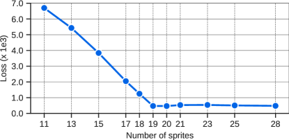
Figure 8: Effect of $K$. We report the loss obtained for varying number of sprites on Tetrominoes, where the ground-truth number of different shapes is 19.

B.2 Effect of $\lambda$

The hyperparameter $\lambda$ controls the weight of the regularization term that counts the number of non-empty sprites used. In Figure 9, we show qualitative results obtained for different values of $\lambda$ on Multi-dSprites. When $\lambda$ is zero or small (here $\lambda=10^{-5}$), the optimization typically falls into bad local minima where multiple layers attempt to reconstruct the same object. Increasing the penalization ($\lambda=10^{-4}$) prevents this phenomenon by encouraging reconstructions using the minimal number of non-empty sprites. When $\lambda=10^{-3}$, the penalization is too strong and some objects are typically missed (last example).

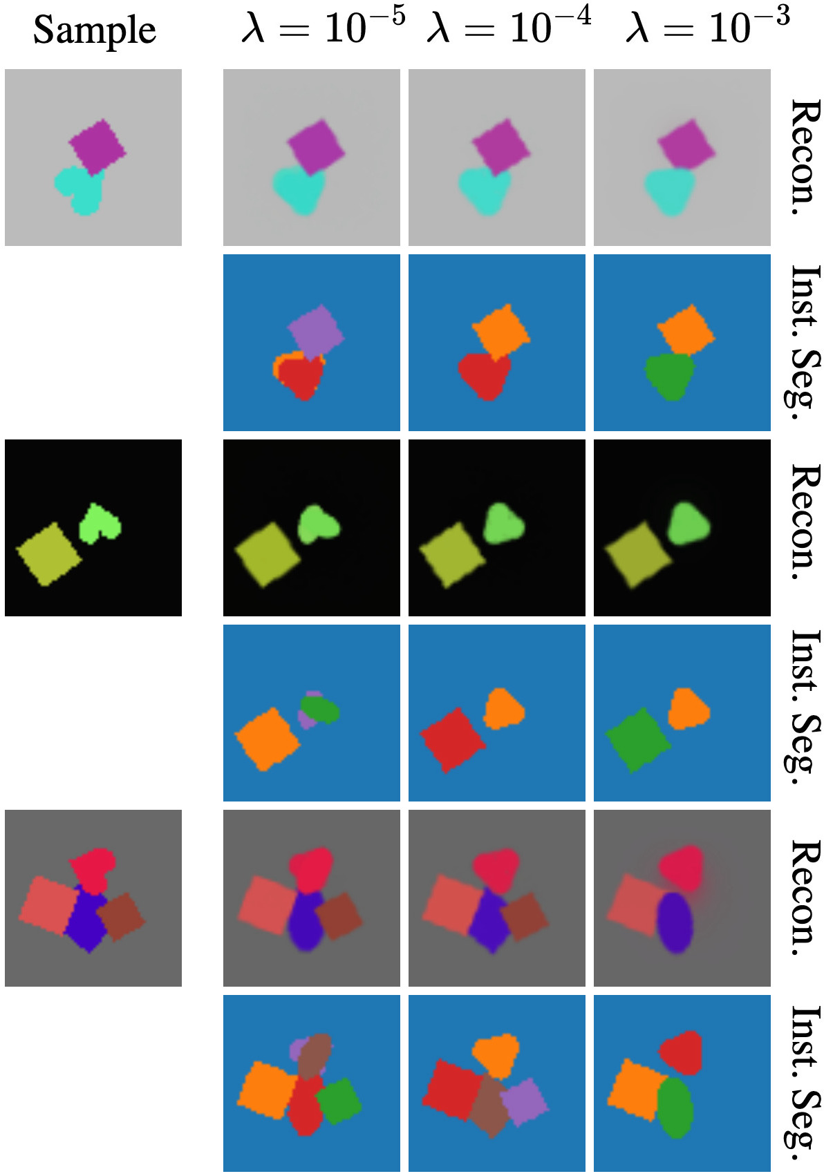
Figure 9: Effect of $\lambda$. We show reconstructions and instance segmentations for different values of $\lambda$ on Multi-dSprites.

B.3 Computational cost

Training our method on Tetrominoes, Multi-dSprites and CLEVR6 respectively takes approximately 5 hours, 3 days and 3.5 days on a single Nvidia GeForce RTX 2080 Ti GPU. Our approach is quite memory efficient and for example on CLEVR6, we can use a batch size of up to 128 on a single V100 GPU with 16GB of RAM as opposed to 4 in [21] and 64 in [49].

Appendix C Training details

The full implementation of our approach and all datasets used are available at https://github.com/monniert/dti-sprites.

C.1 Architecture

We use the same parameter predictor network architecture for all the experiments. It is composed of a shared ResNet [26] backbone truncated after the average pooling and followed by separate Multi-Layer Perceptrons (MLPs) heads predicting sprite transformation parameters for each layer as well as the occlusion matrix. For the ResNet backbone, we use mini ResNet-32 (64 features) for images smaller than $65\times 65$ and ResNet-18 (512 features) otherwise. When modeling large numbers of objects ($>3$), we increase the representation size by replacing the global average pooling by adaptive ones yielding $4\times 4\times 64$ features for mini ResNet-32 and $2\times 2\times 512$ for ResNet-18. Each MLP has the same architecture, with two hidden layers of 128 units.

Table 6: Transformation sequences used.

Dataset	${\mathcal{T}}^{\,\textrm{lay}}$	${\mathcal{T}}^{\,\textrm{spr}}$	${\mathcal{T}}^{\,\textrm{bkg}}$
Tetrominoes [21]	col-pos	-	-
Multi-dSprites [36]	col-pos	sim	col
CLEVR6 [32, 21]	col-pos	proj	col
GTSRB-8 [64]	-	col-proj-tps	col-proj-tps
SVHN [56]	-	col-proj-tps	col-proj-tps
Weizmann Horse [4]	-	col-proj-tps	col-proj-tps
Instagram collections [55]	-	col-proj	col-proj

C.2 Transformation sequences

Similar to DTI-Clustering [55], we model complex image transformations as a sequence of transformation modules which are successively applied to the sprites. Most of the transformation modules we used are introduced in [55], namely affine, projective and TPS modules modeling spatial transformations and a color transformation module. We augment the collection of modules with two additional spatial transformations implemented with spatial transformers [29]:

• a positioning module parametrized by a translation vector and a scale value (3 parameters) and used to model coarse layer-wise object positioning,

• a similarity module parametrized by a translation vector, a scale value and a rotation angle (4 parameters).

The transformation sequences used for each dataset are given in Table 6. All transformations for the multi-object benchmarks are selected to mimic the way images were synthetically generated. For real images, we use the col-proj-tps default sequence when the ground truth number of object categories is well defined and the col-proj sequence otherwise. Visualizing sprites and transformations helps understanding the results and adapting the transformations accordingly.

C.3 Implementation details

Both sprite parameters and predictors are learned jointly and end-to-end using Adam optimizer [37] with a 10^-6 weight decay on the network parameters. Background, sprite appearances and masks are respectively initialized with averaged images, constant value and Gaussian weights. To constrain sprite parameters in values close to $[0,1]$, we use a $\operatorname*{softclip}$ function implemented as a piecewise linear function yielding identity inside $[0,1]$ and an affine function with $0.01$ slope outside $[0,1]$. We experimentally found it tends to work better than (i) a traditional $\operatorname*{clip}$ function which blocks gradients and (ii) a sigmoid function which leads to very small gradients. Similar to [55], we adopt a curriculum learning strategy of the transformations by sequentially adding transformation modules during training at a constant learning rate until convergence, then use a multi-step policy by multiplying the learning rate by $0.1$ once convergence has been reached. For the experiments with a single object on top of a background, we use an initial learning rate of $10^{-3}$ and reduce it once. For the multi-object experiments, because spatial transformations are much stronger, we use an initial value of $10^{-4}$ and first train global layer-wise transformations, using frozen sprites during the first epochs (initialized with constant value for appearances and Gaussian weights for masks). Once such transformations are learned, we learn sprite-specific transformations if any and reduce after convergence the learning rate for the network parameters only. Additionally, in a fashion similar to [55], we perform sprite and predictor reassignment when corresponding sprite has been used for reconstruction less than $20/K\%$ of the images layers. We use a batch size of 32 for all experiments, except for GTSRB-8 and SVHN where a batch size of 128 is used.

C.4 Learning binary masks

There is an ambiguity between learned mask and color values in our raw image formation model. In Figure 10, we show examples of sprites learned following two settings: (i) a raw learning and (ii) a learning where we constrain mask values to be binary. Although learned appearance images $\mathbf{s}^{c}$ (first row) and masks $\mathbf{s}^{\alpha}$ (second row) are completely different, applying the masks onto appearances (third row) yields similar images, and thus similar reconstructions of sample images. However, resulting sprites (last row) demonstrate that the spatial extent of objects is not well defined when learning without any constraint.

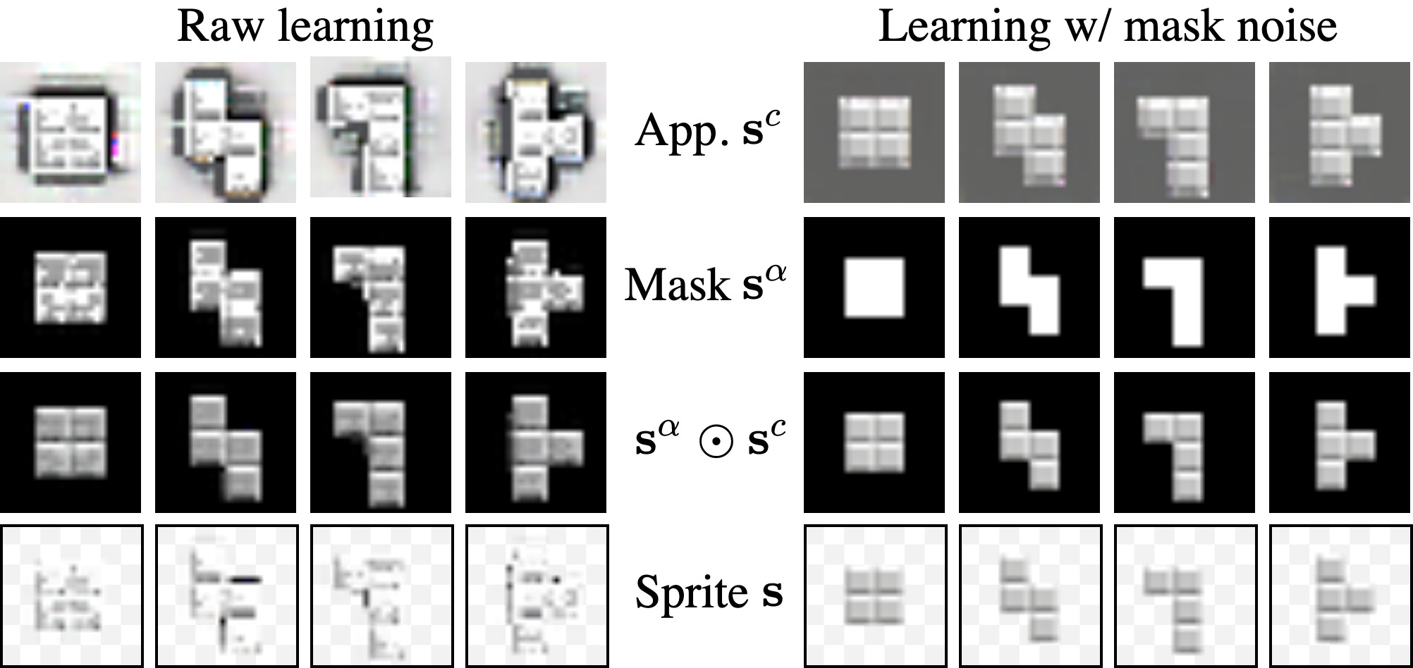
Figure 10: Learning binary masks. We compare results on Tetrominoes obtained with (right) and without (left) injecting noise in masks.

Since constraining the masks to binary values actually resolves ambiguity and forces clear layer separations, we follow the strategy adopted by Tieleman [65] and SCAE [38] to learn binary values, and propose to inject during training uniform noise $\in[-0.4,0.4]$ into the masks before applying our $\operatorname*{softclip}$. Intuitively, such stochasticity prevents the masks from learning appearance aspects and can only be reduced with values close to $0$ and $1$. We experimentally found this approach tends to work better than (i) explicit regularization penalizing values outside of $\{0,1\}$ e.g. with a $x\rightarrow x^{2}(1-x)^{2}$ function and (ii) a varying temperature parameter in a sigmoid function as advocated by Concrete/Gumbel-Softmax distributions [51, 30].

We compare our results obtained with and without injecting noise into the masks on Tetrominoes, where shapes have clear appearances. Quantitatively, while our full model reaches almost a perfect score for both ARI-FG and ARI metrics (resp. 99.6% and 99.8%), these performances averaged over 5 runs are respectively 77.8% and 89.1% when noise is not injected into the masks during learning. We show qualitative comparisons in Figure 10. Note that the masks learned with noise injection are binary and sharp, whereas the ones learned without noise contain some appearance patterns.

Appendix D Additional qualitative results

We provide more qualitative results on the multi-object synthetic benchmarks, namely Tetrominoes (Fig. 11), Multi-dSprites (Fig. 12) and CLEVR6 (Fig. 13). For each dataset, we first show the discovered sprites (at the top), with colored borders to identify them in the semantic segmentation results. We then show 10 random qualitative decompositions. From left to right, each row corresponds to: input sample, reconstruction, semantic segmentation where colors refer to the sprite border colors, instance segmentation where colors correspond to different object instances, and full image decomposition layers where the borders are colored with respect to their instance mask color. Note how we manage to successfully separate the object instances as well as identify their categories and spatial extents.

For additional decompositions, we urge the readers to visit imagine.enpc.fr/~monniert/DTI-Sprites/extra_results.

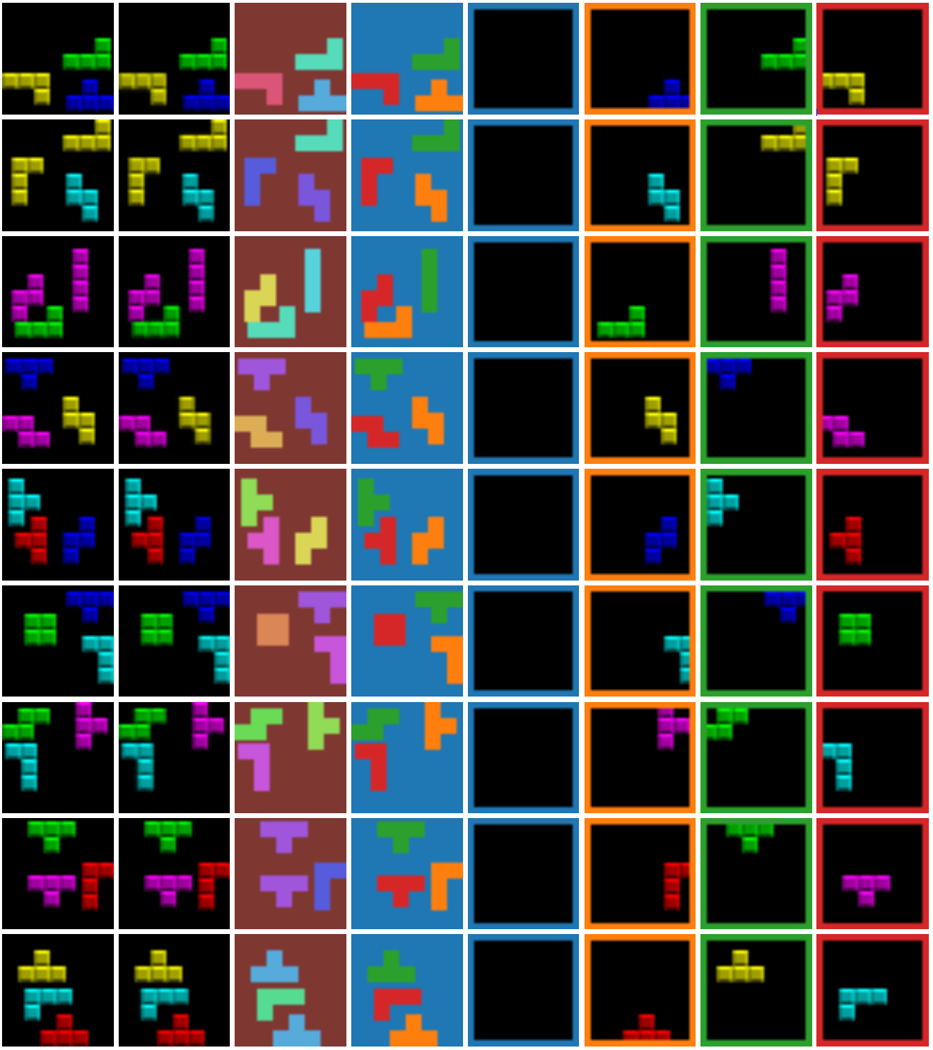
Figure 11: Tetrominoes results. We show discovered sprites (top) and 10 random decomposition results (bottom).

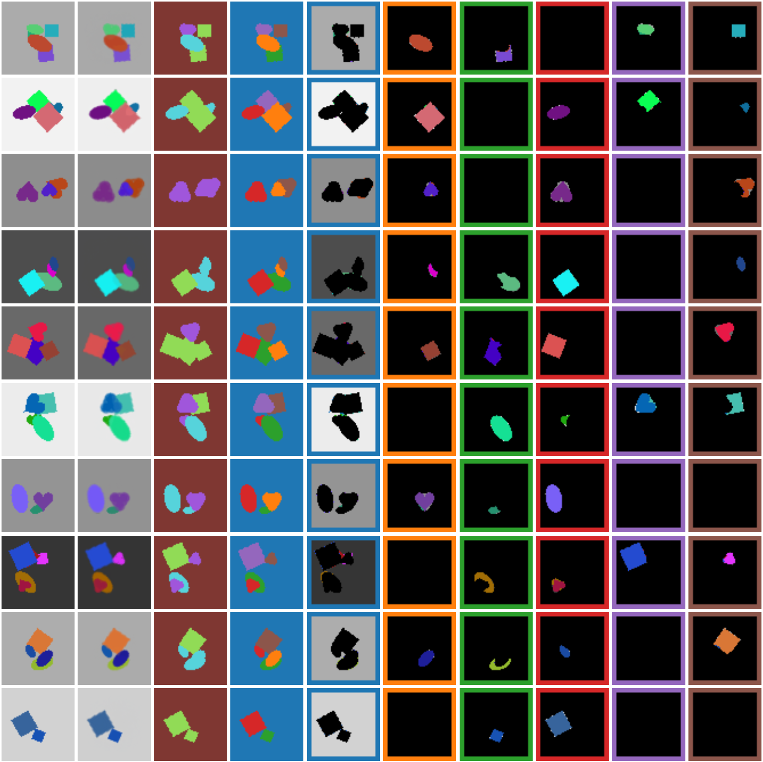
Figure 12: Multi-dSprites results. We show discovered sprites (top) and 10 random decomposition results (bottom).

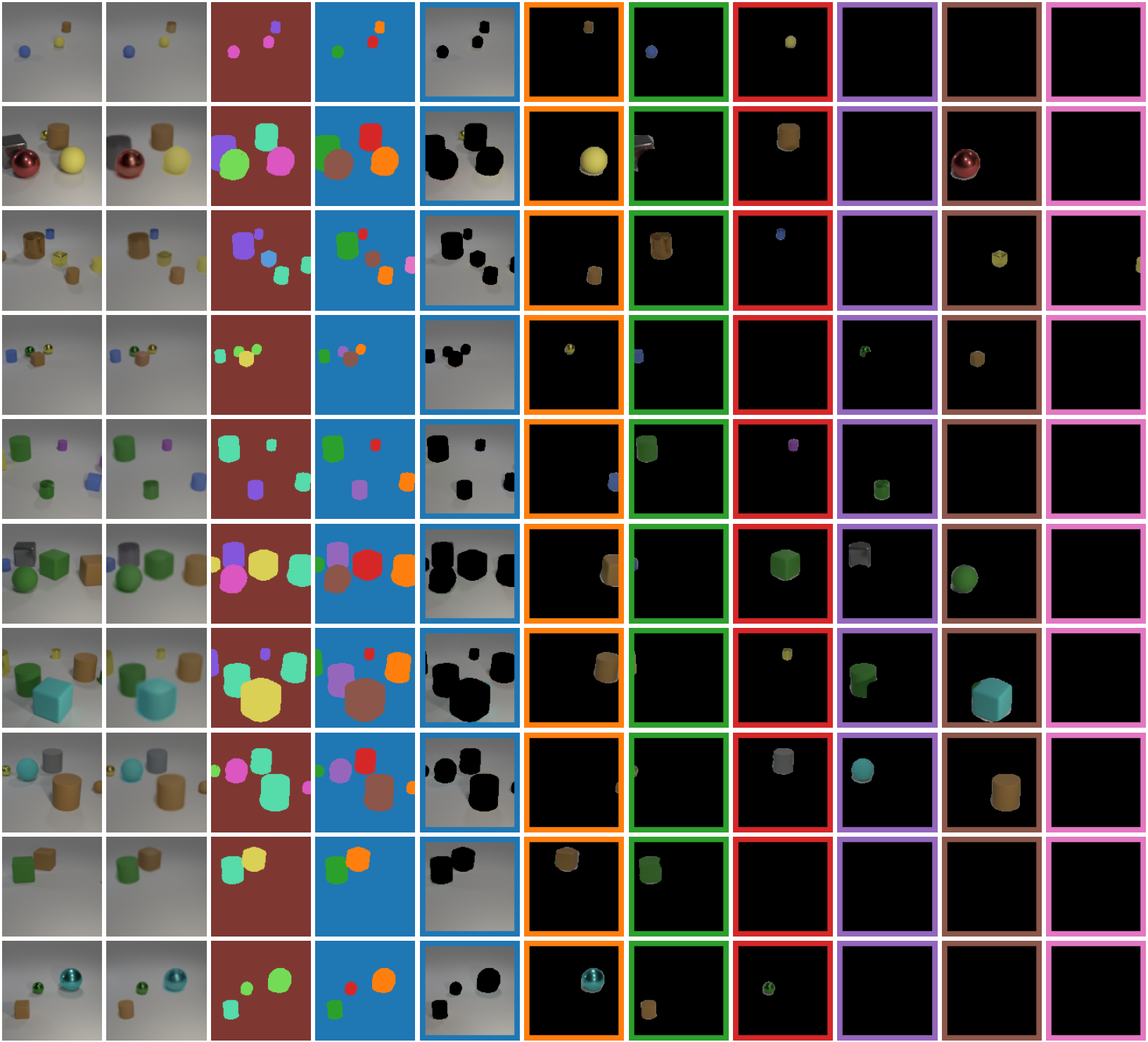
Figure 13: CLEVR6 results. We show discovered sprites (top) and 10 random decomposition results (bottom).

References

- [1] Ankesh Anand, Evan Racah, Sherjil Ozair, Yoshua Bengio, Marc-Alexandre Côté, and R. Devon Hjelm. Unsupervised State Representation Learning in Atari. In NeurIPS, 2019.
- [2] Roberto Annunziata, Christos Sagonas, and Jacques Cali. Jointly Aligning Millions of Images with Deep Penalised Reconstruction Congealing. In ICCV, 2019.
- [3] Relja Arandjelović and Andrew Zisserman. Object Discovery with a Copy-Pasting GAN. arXiv:1905.11369, 2019.
- [4] Eran Borenstein and Shimon Ullman. Learning to Segment. In ECCV, 2004.
- [5] Léon Bottou and Yoshua Bengio. Convergence Properties of the K-Means Algorithms. In NIPS, 1995.
- [6] Christopher P. Burgess, Loic Matthey, Nicholas Watters, Rishabh Kabra, Irina Higgins, Matt Botvinick, and Alexander Lerchner. MONet: Unsupervised Scene Decomposition and Representation. arXiv:1901.11390, 2019.
- [7] Liangliang Cao and Li Fei-Fei. Spatially coherent latent topic model for concurrent object segmentation and classification. In ICCV, 2007.
- [8] Kai-Yueh Chang, Tyng-Luh Liu, and Shang-Hong Lai. From Co-saliency to Co-segmentation: An Efficient and Fully Unsupervised Energy Minimization Model. In CVPR, 2011.
- [9] Mickaël Chen, Thierry Artières, and Ludovic Denoyer. Unsupervised Object Segmentation by Redrawing. In NeurIPS. 2019.
- [10] Minsu Cho, Suha Kwak, Cordelia Schmid, and Jean Ponce. Unsupervised Object Discovery and Localization in the Wild. In CVPR, 2015.
- [11] Mark Cox, Sridha Sridharan, Simon Lucey, and Jeffrey Cohn. Least Squares Congealing for Unsupervised Alignment of Images. In CVPR, 2008.
- [12] Mark Cox, Sridha Sridharan, Simon Lucey, and Jeffrey Cohn. Least-Squares Congealing for Large Numbers of Images. In ICCV, 2009.
- [13] Eric Crawford and Joelle Pineau. Spatially Invariant Unsupervised Object Detection with Convolutional Neural Networks. In AAAI, volume 33, 2019.
- [14] A. P. Dempster, N. M. Laird, and D. B. Rubin. Maximum Likelihood from Incomplete Data via the EM Algorithm. Journal of the Royal Statistical Society, 1977.
- [15] Martin Engelcke, Adam R. Kosiorek, Oiwi Parker Jones, and Ingmar Posner. GENESIS: Generative Scene Inference and Sampling with Object-Centric Latent Representations. In ICLR, 2020.
- [16] S. M. Ali Eslami, Nicolas Heess, Theophane Weber, Yuval Tassa, David Szepesvari, Koray Kavukcuoglu, and Geoffrey E Hinton. Attend, Infer, Repeat: Fast Scene Understanding with Generative Models. In NIPS, 2016.
- [17] Brendan J Frey and Nebojsa Jojic. Estimating Mixture Models of Images and Inferring Spatial Transformations Using the EM Algorithm. In CVPR, 1999.
- [18] Brendan J Frey and Nebojsa Jojic. Transformation-Invariant Clustering Using the EM Algorithm. TPAMI, 2003.
- [19] Ian Goodfellow, Jean Pouget-Abadie, Mehdi Mirza, Bing Xu, David Warde-Farley, Sherjil Ozair, Aaron Courville, and Yoshua Bengio. Generative Adversarial Nets. In NIPS, 2014.
- [20] Kristen Grauman and Trevor Darrell. Unsupervised Learning of Categories from Sets of Partially Matching Image Features. In CVPR, 2006.
- [21] Klaus Greff, Raphaël Lopez Kaufman, Rishabh Kabra, Nick Watters, Chris Burgess, Daniel Zoran, Loic Matthey, Matthew Botvinick, and Alexander Lerchner. Multi-Object Representation Learning with Iterative Variational Inference. In ICML, 2019.
- [22] Klaus Greff, Antti Rasmus, Mathias Berglund, Tele Hao, Harri Valpola, and Jürgen Schmidhuber. Tagger: Deep Unsupervised Perceptual Grouping. In NIPS, 2016.
- [23] Klaus Greff, Rupesh Kumar Srivastava, and Jürgen Schmidhuber. Binding via Reconstruction Clustering. In ICLR Workshops, 2016.
- [24] Klaus Greff, Sjoerd van Steenkiste, and Jürgen Schmidhuber. Neural Expectation Maximization. In NIPS, 2017.
- [25] Philip Häusser, Johannes Plapp, Vladimir Golkov, Elie Aljalbout, and Daniel Cremers. Associative Deep Clustering: Training a Classification Network with no Labels. In GCPR, 2018.
- [26] Kaiming He, Xiangyu Zhang, Shaoqing Ren, and Jian Sun. Deep Residual Learning for Image Recognition. In CVPR, 2016.
- [27] Geoffrey E. Hinton, Alex Krizhevsky, and Sida D. Wang. Transforming Auto-Encoders. In ICANN, 2011.
- [28] Weihua Hu, Takeru Miyato, Seiya Tokui, Eiichi Matsumoto, and Masashi Sugiyama. Learning Discrete Representations via Information Maximizing Self-Augmented Training. In ICML, 2017.
- [29] Max Jaderberg, Karen Simonyan, Andrew Zisserman, and Koray Kavukcuoglu. Spatial Transformer Networks. In NIPS, 2015.
- [30] Eric Jang, Shixiang Gu, and Ben Poole. Categorical Reparameterization with Gumbel-Softmax. In ICLR, 2017.
- [31] Xu Ji, Andrea Vedaldi, and Joao Henriques. Invariant Information Clustering for Unsupervised Image Classification and Segmentation. In ICCV, 2019.
- [32] Justin Johnson, Bharath Hariharan, Laurens van der Maaten, Li Fei-Fei, C Lawrence Zitnick, and Ross Girshick. CLEVR: A diagnostic dataset for compositional language and elementary visual reasoning. In CVPR, 2017.
- [33] Nebojsa Jojic and Brendan J Frey. Learning Flexible Sprites in Video Layers. In CVPR, 2001.
- [34] Armand Joulin, Francis Bach, and Jean Ponce. Discriminative clustering for image co-segmentation. In CVPR, 2010.
- [35] Armand Joulin, Francis Bach, and Jean Ponce. Multi-Class Cosegmentation. In CVPR, 2012.
- [36] Rishabh Kabra, Chris Burgess, Loic Matthey, Raphael Lopez Kaufman, Klaus Greff, Malcolm Reynolds, and Alexander Lerchner. Multi-object datasets. https://github.com/deepmind/multi_object_datasets/, 2019.
- [37] Diederik P. Kingma and Jimmy Ba. Adam: A Method for Stochastic Optimization. In ICLR, 2015.
- [38] Adam Kosiorek, Sara Sabour, Yee Whye Teh, and Geoffrey E Hinton. Stacked Capsule Autoencoders. In NeurIPS, 2019.
- [39] Adam R. Kosiorek, Hyunjik Kim, Ingmar Posner, and Yee Whye Teh. Sequential Attend, Infer, Repeat: Generative Modelling of Moving Objects. In NIPS, 2018.
- [40] H. W. Kuhn and Bryn Yaw. The Hungarian method for the assignment problem. Naval Research Logistic Quarterly, 1955.
- [41] Lucas Lattari, Anselmo Montenegro, and Cristina Vasconcelos. Unsupervised Cosegmentation Based on Global Clustering and Saliency. In ICIP, 2015.
- [42] Erik G Learned-Miller. Data Driven Image Models through Continuous Joint Alignment. TPAMI, 2005.
- [43] Ann B Lee, David Mumford, and Jinggang Huang. Occlusion Models for Natural Images: A Statistical Study of a Scale-Invariant Dead Leaves Model. International Journal of Computer Vision, 2001.
- [44] Bo Li, Zhengxing Sun, Qian Li, Yunjie Wu, and Hu Anqi. Group-Wise Deep Object Co-Segmentation With Co-Attention Recurrent Neural Network. In ICCV, 2019.
- [45] Qi Li, Zhenan Sun, Zhouchen Lin, Ran He, and Tieniu Tan. Transformation invariant subspace clustering. Pattern Recognition, 2016.
- [46] Chen-Hsuan Lin, Ersin Yumer, Oliver Wang, Eli Shechtman, and Simon Lucey. ST-GAN: Spatial Transformer Generative Adversarial Networks for Image Compositing. In CVPR, 2018.
- [47] Zhixuan Lin, Yi-Fu Wu, Skand Vishwanath Peri, Weihao Sun, Gautam Singh, Fei Deng, Jindong Jiang, and Sungjin Ahn. SPACE: Unsupervised Object-Oriented Scene Representation via Spatial Attention and Decomposition. In ICLR, 2020.
- [48] Xiaoming Liu, Yan Tong, and Frederick W Wheeler. Simultaneous Alignment and Clustering for an Image Ensemble. In ICCV, 2009.
- [49] Francesco Locatello, Dirk Weissenborn, Thomas Unterthiner, Aravindh Mahendran, Georg Heigold, Jakob Uszkoreit, Alexey Dosovitskiy, and Thomas Kipf. Object-Centric Learning with Slot Attention. In NeurIPS, 2020.
- [50] J. MacQueen. Some methods for classification and analysis of multivariate observations. Berkeley Symposium on Mathematical Statistics and Probability, 1967.
- [51] Chris J. Maddison, Andriy Mnih, and Yee Whye Teh. The Concrete Distribution: A Continuous Relaxation of Discrete Random Variables. In ICLR, 2017.
- [52] Georges Matheron. Modèle Séquentiel de Partition Aléatoire. Technical report, CMM, 1968.
- [53] Marwan A. Mattar, Allen R. Hanson, and Erik G. Learned-Miller. Unsupervised Joint Alignment and Clustering using Bayesian Nonparametrics. In UAI, 2012.
- [54] Erik G Miller, Nicholas E Matsakis, and Paul A Viola. Learning from One Example Through Shared Densities on Transforms. In CVPR, 2000.
- [55] Tom Monnier, Thibault Groueix, and Mathieu Aubry. Deep Transformation-Invariant Clustering. In NeurIPS, 2020.
- [56] Yuval Netzer, Tao Wang, Adam Coates, Alessandro Bissacco, Bo Wu, and Andrew Y Ng. Reading Digits in Natural Images with Unsupervised Feature Learning. In NIPS Workshop, 2011.
- [57] L. Romaszko, C. K. I. Williams, P. Moreno, and P. Kohli. Vision-as-Inverse-Graphics: Obtaining a Rich 3D Explanation of a Scene from a Single Image. In ICCV Workshops, 2017.
- [58] Michael Rubinstein, Armand Joulin, Johannes Kopf, and Ce Liu. Unsupervised Joint Object Discovery and Segmentation in Internet Images. In CVPR, 2013.
- [59] Jose Rubio, Joan Serrat, Antonio Lopez, and Nikos Paragios. Unsupervised co-segmentation through region matching. In CVPR, 2012.
- [60] Bryan C. Russell, William T. Freeman, Alexei A. Efros, Joseph Sivic, and Andrew Zisserman. Using Multiple Segmentations to Discover Objects and their Extent in Image Collections. In CVPR, 2006.
- [61] Krishna Kumar Singh, Utkarsh Ojha, and Yong Jae Lee. FineGAN: Unsupervised Hierarchical Disentanglement for Fine-Grained Object Generation and Discovery. In CVPR, 2019.
- [62] Joseph Sivic, Bryan C. Russell, Alexei A. Efros, Andrew Zisserman, and William T. Freeman. Discovering objects and their location in images. In ICCV, 2005.
- [63] Josef Sivic, Bryan C. Russell, Andrew Zisserman, William T. Freeman, and Alexei A. Efros. Unsupervised Discovery of Visual Object Class Hierarchies. In CVPR, 2008.
- [64] J. Stallkamp, M. Schlipsing, J. Salmen, and C. Igel. Man vs. computer: Benchmarking machine learning algorithms for traffic sign recognition. Neural Networks, 2012.
- [65] Tijmen Tieleman. Optimizing Neural Networks That Generate Images. PhD Thesis, University of Toronto, 2014.
- [66] Wouter Van Gansbeke, Simon Vandenhende, Stamatios Georgoulis, Marc Proesmans, and Luc Van Gool. SCAN: Learning to Classify Images without Labels. In ECCV, 2020.
- [67] Sjoerd van Steenkiste, Michael Chang, Klaus Greff, and Jürgen Schmidhuber. Relational Neural Expectation Maximization: Unsupervised Discovery of Objects and their Interactions. In ICLR, 2018.
- [68] Ashish Vaswani, Noam Shazeer, Niki Parmar, Jakob Uszkoreit, Llion Jones, Aidan N Gomez, Łukasz Kaiser, and Illia Polosukhin. Attention is All you Need. In NIPS, 2017.
- [69] Sara Vicente, Carsten Rother, and Vladimir Kolmogorov. Object Cosegmentation. In CVPR, 2011.
- [70] Huy V. Vo, Francis Bach, Minsu Cho, Kai Han, Yann LeCun, Patrick Pérez, and Jean Ponce. Unsupervised Image Matching and Object Discovery as Optimization. In CVPR, 2019.
- [71] Huy V. Vo, Patrick Pérez, and Jean Ponce. Toward Unsupervised, Multi-Object Discovery in Large-Scale Image Collections. In ECCV, 2020.
- [72] Julius von Kügelgen, Ivan Ustyuzhaninov, Peter Gehler, Matthias Bethge, and Bernhard Schölkopf. Towards causal generative scene models via competition of experts. In ICLR Workshops, 2020.
- [73] Nicholas Watters, Loic Matthey, Christopher P. Burgess, and Alexander Lerchner. Spatial Broadcast Decoder: A Simple Architecture for Learning Disentangled Representations in VAEs. In ICLR Workshops, 2019.
- [74] John Winn and Nebojsa Jojic. LOCUS: Learning Object Classes with Unsupervised Segmentation. In ICCV, 2005.
- [75] Jiajun Wu, Erika Lu, Pushmeet Kohli, Bill Freeman, and Josh Tenenbaum. Learning to See Physics via Visual De-animation. In NIPS, 2017.
- [76] Jiajun Wu, Joshua B. Tenenbaum, and Pushmeet Kohli. Neural Scene De-rendering. In CVPR, 2017.
- [77] Jianwei Yang, Anitha Kannan, Dhruv Batra, and Devi Parikh. LR-GAN: Layered Recursive Generative Adversarial Networks for Image Generation. In ICLR, 2017.
- [78] Yanchao Yang, Yutong Chen, and Stefano Soatto. Learning to Manipulate Individual Objects in an Image. In CVPR, 2020.
- [79] Hongkai Yu, Min Xian, and Xiaojun Qi. Unsupervised co-segmentation based on a new global GMM constraint in MRF. In ICIP, 2014.