Nonparametric Difference-in-Differences in Repeated Cross-Sections with Continuous Treatments

Abstract

This paper studies the identification of causal effects of a continuous treatment using a new difference-in-difference strategy. Our approach allows for endogeneity of the treatment, and employs repeated cross-sections. It requires an exogenous change over time which affects the treatment in a heterogeneous way, stationarity of the distribution of unobservables and a rank invariance condition on the time trend. On the other hand, we do not impose any functional form restrictions or an additive time trend, and we are invariant to the scaling of the dependent variable. Under our conditions, the time trend can be identified using a control group, as in the binary difference-in-differences literature. In our scenario, however, this control group is defined by the data. We then identify average and quantile treatment effect parameters. We develop corresponding nonparametric estimators and study their asymptotic properties. Finally, we apply our results to the effect of disposable income on consumption.

Keywords: identification, repeated cross-sections, nonlinear models, continuous treatment, random coefficients, endogeneity, difference-in-differences.

1 Introduction

Differences-in-Differences (DID) is arguably one of the most popular methods for policy evaluation. In its standard version, it allows to identify the causal effect of a binary treatment on a given outcome, even when units are not allocated randomly to the treatment. The idea is to compare the evolution of the average outcome of the treatment group, which receives a treatment after a certain date, with that of the control group, which remains untreated. The DID strategy builds on the so-called common trend assumption, viz. the assumption that the changes in $Y(0)$, the potential outcome absent the treatment, are identical between the treatment and the control group. One way to see this condition is that treatment changes should be exogenous in that they are not related to changes in $Y(0)$. Under common trends, the average time trend on $Y(0)$ can be identified using the control group, as this group does not experience the effect of the treatment. Once this time trend is accounted for, we can identify the average treatment effect by a simple before-after comparison on the treatment group.

A crucial limitation of the standard DID framework is that the treatment is required to be binary. Yet, in many cases, units experience various treatment intensities, and not just a zero-one treatment. Examples include, among many others, unemployment benefits, specific public expenditures (e.g., hospitals expenditure per capita, teacher’s wages), changes in prices, in income etc. Usual solutions in such cases are to either consider a linear model or to discretize the treatment. Both solutions are problematic. In the first case, the model cannot account for, e.g., unobservable terms affecting both treatment intensity and treatment effects, effectively assuming that the treatment has the same effect for every level of treatment intensity. In the second case, discretization introduces arbitrariness and leads to an information loss. E.g., after discretization, even vastly different income changes would be assumed to have the same effect, because all that matters is the fact that they change. This makes the DID framework not useful to study, e.g., causal marginal propensities to consume out of income, because individuals at low levels of income are more likely to face liquidity constraints than individuals at high levels, and the size of the income change arguably matters (see, e.g., Hsieh, 2003).

In this paper, we propose a solution that circumvents these issues. Specifically, we show identification of several treatment effect parameters, allowing for nonlinear and heterogeneous effects of the treatment without imposing functional form restrictions (e.g., linearity), nor any discretization. We also allow for heterogeneous time trends on potential outcomes. This is important, since assuming the same time trends for all units may be overly restrictive. Firms or individuals with different productivities may be affected differently by macroeconomic shocks, for instance.

The idea behind our identification strategy retains the spirit of the DID approach. We use the fact that the distribution of the treatment, in our case a continuous random variable, changes over time for some exogenous reason, yet some units remain at the same level of treatment. In our approach, the latter units form the control group, which allows us to identify the (heterogeneous) time trend on potential outcomes. Once this time trend has been removed, the distribution of the appropriately modified potential outcome does not vary over time any longer. Then, any difference over time in the distribution of the modified, observed outcome should be solely due to the treatment. With this insight, we can identify causal effects of the treatment.

To make this strategy operational, we rely on three main assumptions. First, we assume that units sharing the same rank in the distribution of the treatment at two different periods have the same distribution of the unobservables governing potential outcomes. This assumption is related to the aforementioned exogeneity of the change in the distribution of the treatment over time. It first ensures that groups, similar to the control and treatment group with binary treatments, may be defined through the ranking of the treatment. With this construction of groups, the condition becomes almost the same as Assumptions 1 and 3 in Athey and Imbens (2006), on which our paper builds to identify (heterogeneous) time trends. Second, we assume that a unit with stable unobservables in two different periods will also have the same ranking in the distributions of potential outcome in these two periods. Again, this assumption is identical to Assumption 2 in Athey and Imbens (2006). Third, we suppose that the change in the distribution of the treatment is heterogeneous, in the sense that the cumulative distribution functions (cdfs) of the treatment variable between the two periods cross. This crossing point defines the control group and allows us to identify the heterogeneous time trends.

Despite some similarities with the nonlinear difference-in-differences setting of Athey and Imbens (2006), our continuous treatment set-up exhibits several important distinct features. First, Athey and Imbens (2006) focus on the binary treatment case, while we consider a continuous treatment. Second, our control group is determined by the data rather than fixed ex ante. While our paper also shares some similarities with the paper by de Chaisemartin and D’Haultfœuille (2018), the framework and identification strategy is nonetheless very different: In particular, de Chaisemartin and D’Haultfœuille (2018) focus on binary (or ordered) treatments. With a continuous treatment, their strategy would require to have a control group for which the whole distribution of the treatment variable would remain unchanged over time, an assumption unlikely to be satisfied in practice. In contrast, we only require the distribution of the treatment to change in such a way that there exists a crossing point. A change in the mean and the variance of a normal distribution, for instance, satisfies this requirement.

We consider several extensions to our main setup. First, we show how covariates can be included into our analysis. Second, we establish that our model extends in a straightforward way to multidimensional continuous treatments. Third, we show that while a number of parameters cannot be point identified, basically because time only provides us with limited exogenous variations, they can be partially identified using weak local curvature conditions. Finally, we prove that under functional form restrictions that still allow for ample heterogeneity, we can point identify all marginal effects.

Based on this extensive identification analysis, we also develop nonparametric sample counterparts estimators. While our estimators of the average and quantile effects involve several nonparametric steps, each one of these steps is straightforward to perform. We show the asymptotic normality of the estimators. When the “control group” corresponds to a single point of support of the continuous treatment, the estimators are not root-n consistent, but converge at standard univariate nonparametric rates.

Finally, we apply our methodology to analyze the marginal propensity to consume in the US. We exploit for that purpose a change in the schedule of the Earned Income Tax Credit (EITC) between 1987 and 1989. We argue that this change generates exactly the crossing condition we require. Applying our method, we obtain an estimated time trend that displays heterogeneity, underlying the need to go beyond mere additive time trends. Moreover, our estimates of the marginal effects suggest that low-income individuals increase substantially their consumption (by around 50%), while medium-income individuals would not significantly adjust their consumption. This is in line with many findings in the literature, see e.g., Johnson et al. (2006) and Kaplan and Violante (2014).

The paper is organized as follows. In Section 2, we introduce the model formally, discuss the parameters of interest and provide our main identification results. The extensions considered above are discussed in Section 3. Section 4 is devoted to estimation. Section 5 presents the application, and Section 6 concludes. All proofs are gathered in the appendix.

2 Model and Main Identification Results

2.1 Assumptions

We consider a potential outcome framework with a continuous treatment. The potential outcome at period $t$, corresponding to a treatment $x\in\mathcal{X}\subset\mathbb{R}$, is denoted by $Y_{t}(x)$, with $Y_{t}(x)\in\mathbb{R}$. We observe, at each period $t\in\{1,...,T\}$, the actual treatment $X_{t}$ and the corresponding outcome, $Y_{t}\equiv Y_{t}(X_{t})$. We are particularly interested in the average and quantile treatment on the treated effects:

$$\Delta^{ATT}(x,x^{\prime}) \equiv E\left[Y_{T}(x^{\prime})-Y_{T}(x)|X_{T}=x\right],$$

$$\Delta^{QTT}(p,x,x^{\prime}) \equiv F_{Y_{T}(x^{\prime})|X_{T}}^{-1}(p|x)-F_{Y_{T}(x)|X_{T}}^{-1}(p|x),$$

for any $x$ and $x^{\prime}$ in the support $\text{Supp}(X_{T})$ of $X_{T}$. Here, $F_{A|B}(a|b)$ denotes the conditional cdf of a random variable $A$ at $a$, given that a random vector $B$ takes the value $b$, and $F_{A|B}^{-1}(\tau|b)$ denotes its inverse, the $\tau$-conditional quantile function. We henceforth focus on the effects at period $T,$ because they are the most natural to compute in general, but we can identify similar effects at any date.

The main issue in identifying the parameters above is endogeneity of the actual treatment, i.e., $X_{t}$ may depend on $(Y_{t}(x))_{x\in\mathcal{X}}$. In such a case, naive estimators do not coincide with the average and quantile treatment effects defined above. For instance, $E(Y_{T}|X_{T}=x^{\prime})-E(Y_{T}|X_{T}=x)\neq\Delta^{ATT}(x,x^{\prime})$. Our idea for identifying these causal parameters, then, is to use exogenous changes in $X_{t}$ (due to, e.g., a policy change), and apply a difference-in-difference type strategy. To make this idea operational, we restrict the way time affects both observed and unobserved variables by imposing three main restrictions. The first restriction is a stationarity condition on the observed and unobserved determinants of the outcome. The second restriction limits the way time affects the outcome itself. The third restriction affects the way the distribution of $X_{t}$ changes over time. We discuss them in turn using the notation $V_{t}=F_{X_{t}}(X_{t})$ to denote the rank of an individual in the distribution of the treatment.

Assumption 1.

(stationarity of unobservables) For all $t\in\{1,...,T\}$, $Y_{t}(x)=g_{t}(U_{t}(x))$ where for all $(x,v)\in\mathcal{X}\times[0,1]$ the distribution of the unobserved variable $U_{t}(x)|V_{t}=v$ does not depend on $t$.

We can interpret this assumption as follows. First, it defines implicitly groups, similar to control and treatment groups with binary treatments, through the rank variable $V_{t}$. Then, we assume that within each group, unobserved terms related to potential outcomes have a time-invariant distribution. This latter condition is similar to Assumptions 3.1 and 3.3 in Athey and Imbens (2006), where the authors also assume that within both the control and the treatment group the distribution of the unobserved term related to $Y_{t}(0)$ is constant over time.

Importantly, Assumption 1 does not restrict the cross-sectional dependence between $U_{t}(x)$ and $V_{t}$, which is at the core of the endogeneity problem we face in this scenario. On the other hand, it rules out changes in the type of endogeneity, as the distribution of $(U_{t}(x),V_{t})$ is supposed to be time invariant. In our application below, $X_{t}$ corresponds to disposable income. The tax rate affects disposable income, but a change in the tax rate is unlikely to change the ranking of individuals in the income distribution, holding other characteristics constant (e.g., the number of household members). In other applications, this condition may be more restrictive. We discuss this point further when we draw a parallel with instrumental variable models in Section 2.4.2 below.

The following assumption specifies the second requirement mentioned above:

Assumption 2.

(rank invariance on the time trend) For all $(x,t)\in\mathcal{X}\times\{1,...,T\}$, $U_{t}(x)\in\mathbb{R}$ and $g_{t}$ is strictly increasing. Without loss of generality, we let $g_{T}(y)=y$ for all $y\in\text{Supp}(Y_{T})$.

Assumption 2 is again materially identical to Assumption 3.2 in Athey and Imbens (2006). Combined with Assumption 1, it states that an individual that has the same unobservable in two different periods (i.e., $U_{t}(x)\equiv U_{t^{\prime}}(x)$) will also have the same ranking in the distributions of potential outcomes $Y_{t}(x)$ and $Y_{t^{\prime}}(x)$ in the same two periods. Assumption 2 generalizes the standard translation model $g_{t}(u)=\delta_{t}+u$ to allow for heterogeneous time trends. This can be important in some applications. For instance, macroeconomic shocks may have different effects on high- and low-wage earners. Note that given the strict monotonicity condition, we can always make the normalization $g_{T}(y)=y$, by just redefining $U_{t}(x)$ as $g_{T}(U_{t}(x))$ and $g_{t}(y)$ as $g_{t}\circ g_{T}^{-1}(y)$.

Assumption 3.

(crossing points) For all $t\in\{1,...,T-1\}$, there exists $x_{t}^{\ast}\in\mathbb{R}$ such that $F_{X_{t}}(x_{t}^{\ast})=F_{X_{T}}(x_{t}^{\ast})\in(0,1)$.

Contrary to Assumptions 1-2, Assumption 3 only involves observables, and is therefore directly testable in the data. It means, roughly speaking, that the exogenous change (induced by, e.g., a policy change) affects individuals’ treatment in a heterogeneous way. Requiring time to have a heterogeneous effect on the treatment is also required in the usual difference-in-difference strategy, and a similar condition is required in fuzzy settings considered by de Chaisemartin and D’Haultfœuille (2018).

Note that $x_{t}^{\ast}$ can be identified and estimated using the data. We consider such an estimator in Section 4 below. However, sometimes the value of the crossing point may also be inferred from the design of the policy change. Comparing the theoretical crossing point with the crossing point obtained from the data then constitutes a check for the hypothesis that the policy change has not changed the distribution of the unobservables. We refer to the application below for more details about this.

Two additional remarks on Assumption 3 are in order. First, this assumption holds if $F_{X_{t}}$ remains constant with $t$. In this case, however, we identify only the trivial parameters $\Delta^{ATT}(x,x)=\Delta^{QTT}(p,x,x)=0$. Second, we assume for simplicity crossings between the cdf of $X_{T}$ and all other cdfs, but actually, $T-1$ crossings are sufficient, provided that we can “relate” them to each other, for instance if the cdf of $X_{t}$ crosses that of $X_{t+1}$ for $1\leq t<T$. Also, with only one crossing between $F_{X_{s}}$ and $F_{X_{t}}$, we still identify some treatment effects at periods $s$ or $t$, following the same logic as in Section 2.3 below. So even if Assumption 3 does not make this apparent, adding periods help because it increases the odds of having at least one crossing point, which is sufficient for identifying some causal parameters.

The last assumption we impose is a regularity condition:

Assumption 4.

(regularity conditions) For all $t\in\{1,...,T\}$, $E(|Y_{t}|)<\infty$ and $F_{X_{t}}$ is continuous on $\text{Supp}(X_{t})$, which is an interval included in $\mathcal{X}$. For all $x^{\prime}\in\text{Supp}(X_{t})$ and $u\in\text{Supp}(U_{t}(x^{\prime}))$, there exist versions of $E[Y_{t}|X_{t}]$ and $P^{U_{t}(x^{\prime})|V_{t}}$ such that $x\mapsto E[Y_{t}|X_{t}=x]$ and $v\mapsto F_{U_{t}(x^{\prime})|V_{t}}(u|v)$ are continuous.

The continuity conditions are mild, yet important to define properly conditional expectations or cdfs (e.g., $E[Y_{t}|X_{t}=x_{t}^{\ast}]$ or $F_{Y_{t}|X_{t}}(y|x_{t}^{\ast})$).

2.2 Examples

To better understand the types of data generating processes which our assumptions permit, we consider two examples of workhorse models.

2.2.1 Simple Linear Systems

Let us suppose that

$$Y_{t}(x) =\alpha_{t}+x\beta+U_{t},$$ (2.1)

$$X_{t} =\gamma_{t}+\delta_{t}\eta_{t},$$ (2.2)

where $(\alpha_{t},\beta,\gamma_{t},\delta_{t})$ are constants and the marginal distribution of $(U_{t},\eta_{t})$ is assumed constant over time. Suppose also that $\text{Supp}(\eta_{t})=\mathbb{R}$ and $\delta_{t}\neq\delta_{T}$ for all $t\neq T$. Then, Assumptions 1-3 hold with $U_{t}(x)=x\beta+U_{t}$, $g_{t}(u)=\alpha_{t}+u$ and $x_{t}^{\ast}=(\gamma_{t}-\gamma_{T})/(\delta_{T}-\delta_{t})$. Assumption 4 holds under mild restrictions on the distribution of $(U_{t},\eta_{t})$. Note that the model allows for any dependence between $U_{t}$ and $\eta_{t}$. Thus, $X_{t}$ is endogenous in general in the outcome equation, and we cannot recover $\beta$ directly by the OLS. Note, moreover, that we cannot use time as an instrumental variable in the outcome equation either, because it has a direct effect on $Y_{t}$, so none of the standard tools work.

As mentioned above, if the policy change has a pure location effect on $X_{t}$, so that $\delta_{t}=\delta_{T}$ for all $t$, then Assumption 3 is not satisfied. We require to have individuals unaffected by the change, and this holds with a change in scale in (2.2).

Note that we did not impose any condition on the dependence between $(U_{s},\eta_{s})$ and $(U_{t},\eta_{t})$. Hence, the model allows for any form of serial dependence of the unobservables. On the other hand, models with a lagged dependent variable are typically ruled out by our assumptions. To see this, suppose that we replace (2.1) by

$$Y_{t}(x)=\alpha_{t}+x\beta+\rho Y_{t-1}+U_{t}.\\$$ (2.3)

Then,

$$Y_{t}(x)=\widetilde{\alpha}_{t}+\beta x+\widetilde{U}_{t}$$

with $\widetilde{\alpha}_{t}=\alpha+\sum_{k=1}^{\infty}\rho^{k}\left[\alpha_{t-k}+\beta\gamma_{t-k}\right]$ and $\widetilde{U}_{t}=U_{t}+\sum_{k=1}^{\infty}\rho^{k}[\beta\delta_{t-k}\eta_{t-k}+U_{t-k}]$. Therefore, the distribution of $\widetilde{U}_{t}$ depends on $t$ in general, unless $\rho=0$. Then,

$$F_{Y_{t}(x)}^{-1}\circ F_{Y_{t^{\prime}}(x)}(y)=\widetilde{\alpha}_{t}+\beta x+F_{\widetilde{U}_{t}}^{-1}\circ F_{\widetilde{U}_{t^{\prime}}}(y-\alpha_{t^{\prime}}^{\prime}-\beta x),$$

which depends on $x$ in general when $\beta\neq 0$ and $\rho\neq 0$. On the other hand, Assumptions 1-2 imply that for any $(t,t^{\prime})$, $F_{Y_{t}(x)}^{-1}\circ F_{Y_{t^{\prime}}(x)}(y)$ does not depend on $x$. In other words, Assumptions 1-2 are violated in general when $\rho\neq 0$.

This feature is not specific to our assumptions. A similar issue arises in the standard difference-in-differences setup. To see this, consider model (2.3) again, but now with a binary treatment, for which $X_{t}=0$ for all $t\leq 1,$ and $X_{2}=G$, the dummy of being in the treatment group as opposed to the control group in the second period. Suppose, moreover, that $E(U_{t}|G)$ does not depend on $t$. In the case of $\rho=0$, the common trend condition is satisfied with $E(Y_{2}(0)|G)-E(Y_{1}(0)|G)=\alpha_{2}-\alpha_{1}$. But if $\rho\neq 0$, then the common trends assumptions fails to hold in general, since

$$E(Y_{2}(0)|G)-E(Y_{1}(0)|G=0)=\alpha_{2}-\alpha_{1}+\sum_{k=1}^{\infty}\rho^{k}\alpha_{1-k}+\frac{\rho}{1-\rho}E(U_{1}|G),$$

which depends on $G$.

2.2.2 Quantile Regression Type Models

The previous model does not allow for heterogeneous treatment effects or heterogeneous time trends on potential outcomes. We may, however, analyze models with heterogeneous features as they are compatible with our assumptions. The following model exemplifies this:

$$Y_{t} =f_{t}\left[\alpha(U_{t})+X_{t}\beta(U_{t})\right]$$

$$X_{t} =h_{t}(\eta_{t}),$$

where we assume that the marginal distribution of $(U_{t},\eta_{t})$ is constant over time, $\text{Supp}(\eta_{t})=\mathbb{R}$, and for all $t\neq T$, there exists $e_{t}$ such that $h_{t}(e_{t})=h_{T}(e_{t})$. We also assume that $f_{t}$ and $e\mapsto\alpha(e)+x\beta(e)$ are strictly increasing. In this scenario, Assumptions 1-3 are satisfied, with $U_{t}(x)=f_{T}(x\beta(U_{t}))$ and $g_{t}(y)=f_{t}\circ f_{T}^{-1}(y)$. Contrary to the previous example, this model allows for both heterogeneous treatment effects, through the random coefficient $\beta(U_{t})$, and an heterogeneous time trend, through the function $f_{t}$. In the special case where $f_{t}(y)=y+\gamma_{t}$, the model is a linear correlated random coefficients model. Note that even with such a restriction on $f_{t}$, the treatment effect function $e\mapsto\beta(e)$ cannot be identified through standard quantile regression of $Y_{t}$ on $X_{t}$, because of the dependence between $X_{t}$ and $U_{t}$.

2.3 Main Identification Results

Our identification strategy works in two steps: In the first step, we identify the effect of time on the outcome, i.e., the function $g_{t}$. This implies that we identify $\widetilde{Y}_{t}=g_{t}^{-1}(Y_{t})$, whose distribution does not depend on time anymore (conditional on $V_{t})$. Then, in a second step, we can use time as an instrument to recover specific causal effects. For ease of exposition, we first outline our method in the case of $T=2$.

2.3.1 Step 1: Identification of the Time Trend

To recover $g_{1}$, we rely on observations at the crossing point, i.e. observations for whom $X_{1}=x_{1}^{\ast}$. Under Assumptions 1-4, the following is true:

$$P\left(Y_{2}\leq y|X_{2}=x_{1}^{\ast}\right) \overset{A.2}{=}P\left(U_{2}(x_{1}^{\ast})\leq y|V_{2}=F_{X_{2}}(x_{1}^{\ast})\right)$$

$$\overset{A.1}{=}P\left(U_{1}(x_{1}^{\ast})\leq y|V_{1}=F_{X_{2}}(x_{1}^{\ast})\right)$$

$$\overset{A.3}{=}P\left(U_{1}(x_{1}^{\ast})\leq y|V_{1}=F_{X_{1}}(x_{1}^{\ast})\right)$$

$$\overset{A.2}{=}P\left(g_{1}(U_{1}(x_{1}^{\ast}))\leq g_{1}(y)|X_{1}=x_{1}^{\ast}\right)$$

$$=P\left(Y_{1}\leq g_{1}(y)|X_{1}=x_{1}^{\ast}\right),$$ (2.4)

where we indicate the respective assumptions employed by superscripts upon equalities. As a result, $g_{1}$ is identified by

$$g_{1}(y)=F_{Y_{1}|X_{1}}^{-1}\left[F_{Y_{2}|X_{2}}(y|x_{1}^{\ast})|x_{1}^{\ast}\right].$$ (2.5)

Hence, under our assumptions, the time trend $g_{1}$ can be identified using observations for which $X_{1}=x_{1}^{\ast}$ and $X_{2}=x_{1}^{\ast}$. These two sets of observations, though distinct as we use repeated cross sections, have the same distribution of unobservables and the same value of the treatment. Therefore, differences between the distributions of outcomes can only stem from the effect of time itself. This idea is very similar to that used in difference-in-differences, where the control group permits the identification of the (common) time trend. For this reason, in what follows we classify all observations satisfying $X_{1}=x_{1}^{\ast}$ to form the “control group”.

Note that our model allows for heterogeneous time trends. As Athey and Imbens (2006), we therefore recover a whole function $g_{1}$ rather than a single coefficient for the time trend, as in the standard difference-in-differences model. Also as Athey and Imbens (2006), we identify $g_{1}$ by a quantile-quantile transform. When it comes to the identification of the time trend, the main difference between our approach and that of Athey and Imbens (2006) lies in how the control group is defined. While it is defined ex ante in Athey and Imbens (2006), it is data-driven and defined through the crossing points here.

Beyond the identification of $g_{1}$, (2.5) reveals that the model is testable, if there are several crossing points between $F_{X_{1}}$ and $F_{X_{2}}$, say $x_{1}^{\ast}$ and $x_{1}^{\ast\ast}$. In such a case, our model implies indeed that for all $y$,

$$F_{Y_{1}|X_{1}}^{-1}\left[F_{Y_{2}|X_{2}}(y|x_{1}^{\ast})|x_{1}^{\ast}\right]=F_{Y_{1}|X_{1}}^{-1}\left[F_{Y_{2}|X_{2}}(y|x_{1}^{\ast\ast})|x_{1}^{\ast\ast}\right],$$

which is a testable restriction. Related to this, if the true set of crossing points is an interval $I$, say, we have $F_{X_{1}|X_{1}\in I}=F_{X_{2}|X_{2}\in I}$. Then, integrating (2.4) over $x_{1}^{*}\in I$, we obtain

$$P\left(Y_{2}\leq y|X_{2}\in I\right)=P\left(Y_{1}\leq g_{1}(y)|X_{1}\in I\right).$$

Therefore, $g_{1}(y)=F^{-1}_{Y_{1}|X_{1}\in I}\left[F_{Y_{2}|X_{2}\in I}(y)\right]$, which implies that $g_{1}$ could be in principle estimated at a parametric rather than nonparametric rate in this case.

2.3.2 Step 2: Identification of ATT and QTT

Next, we consider the identification of the treatment effects $\Delta^{ATT}(x,x^{\prime})$ and $\Delta^{QTT}(p,x,x^{\prime})$. Start out by considering the transformed potential and observed outcomes $\widetilde{Y}_{t}(x)=g_{t}^{-1}(Y_{t}(x))$ and $\widetilde{Y}_{t}=g_{t}^{-1}(Y_{t})$ for $t=1,2$. By virtue of Assumption 1, $F_{\widetilde{Y}_{1}(x)}=F_{\widetilde{Y}_{2}(x)}$. Time can thus be seen as an instrument for the treatment: while it affects the treatment (or its distribution, to be precise), it has no direct effect on potential outcomes. The same idea is used in a different DID framework by de Chaisemartin and D’Haultfœuille (2018).

To proceed with the identification of our model, let $q_{t}=F_{X_{t}}^{-1}\circ F_{X_{T}}$. Thus, $q_{t}(x)$ denotes the value of $X_{t}$ (say, income in period $t$) for an individual at the same rank as another individual whose period $T$ income is $X_{T}=x$. Then,

$$E\left[\widetilde{Y}_{1}|X_{1}=q_{1}(x)\right] = E\left[U_{1}(q_{1}(x))|V_{1}=F_{X_{2}}(x)\right]$$

$$\overset{A.1}{=} E\left[U_{2}(q_{1}(x))|V_{2}=F_{X_{2}}(x)\right]$$

$$= E\left[U_{2}(q_{1}(x))|X_{2}=x\right].$$

By the normalization $g_{2}(y)=y$, the latter is the mean counterfactual outcome at period 2 for individuals with $X_{2}=x$ if $X_{2}$ was moved exogenously to $q_{1}(x)$. We can therefore identify $\Delta^{ATT}(x,q_{1}(x))$, the average effect of moving $X_{2}$ from their initial value $x$ to $q_{1}(x)$, by

$$\Delta^{ATT}(x,q_{1}(x)) \overset{A.2}{=} E\left[U_{2}(q_{1}(x))-U_{2}(x)|X_{2}=x\right]$$

$$= E\left[\widetilde{Y}_{1}|X_{1}=q_{1}(x)\right]-E\left[\widetilde{Y}_{2}|X_{2}=x\right].$$

This means that we can obtain $\Delta^{ATT}(x,x^{\prime})$ for any pair $(x,x^{\prime})$ such that $x^{\prime}=q_{1}(x)$.

Similarly, we have, for any $p\in(0,1)$,

$$F_{\widetilde{Y}_{1}|X_{1}}^{-1}(p|q_{1}(x)) = F_{U_{1}(q_{1}(x))|V_{1}}^{-1}(p|F_{X_{2}}(x))$$

$$\overset{A.\ref{hyp:stationarity}}{=} F_{U_{2}(q_{1}(x))|V_{2}}^{-1}(p|F_{X_{2}}(x))$$

$$\overset{A.\ref{hyp:direct_effect}}{=} F_{Y_{2}(q_{1}(x))|X_{2}}^{-1}(p|x).$$

This implies that

$$\Delta^{QTT}(p,x,q_{1}(x))=F_{\widetilde{Y}_{1}|X_{1}}^{-1}(p|q_{1}(x))-F_{\widetilde{Y}_{2}|X_{2}}^{-1}(p|x).$$

Theorem 1 summarizes our findings so far, and generalizes it to any value of $T$.

Theorem 1.

Under Assumptions 1-4, we identify, for all $x\in\text{Supp}(X_{T})$, $p\in(0,1)$ and $t\in\{1,...,T-1\}$, the functions $g_{t}$ and the average and quantile treatment effects $\Delta^{ATT}(x,q_{t}(x))$ and $\Delta^{QTT}(p,x,q_{t}(x))$.

Note that if $x\mapsto Y_{T}(x)$ is differentiable, we have, by the mean value theorem,

$$Y_{T}(q_{t}(x))-Y_{T}(x)=Y^{\prime}_{T}(\widetilde{X})(q_{t}(x)-x),$$

for some random term $\widetilde{X}\in[x,q_{t}(x)]$. As a result, by Theorem 1, we identify

$$\Delta^{AME}_{\text{app}}(x)\equiv E[Y_{T}^{\prime}(\widetilde{X})|X_{T}=x]=\frac{\Delta^{ATT}(x,q_{t}(x))}{q_{t}(x)-x}.$$ (2.6)

In other words, $\Delta^{ATT}(x,q_{t}(x))/(q_{t}(x)-x)$ may be interpreted as an average marginal effect for units at $X_{T}=x$. Contrary to usually, however, the derivative of $Y_{T}(.)$ is not evaluated at the current treatment value $x$, but at another point $\widetilde{X}\in(x,q_{t}(x))$. If $q_{t}(x)$ is close to $x$ or $Y_{T}$ is close to being linear, we can nevertheless expect $Y_{T}^{\prime}(\widetilde{X})$ to be close to the usual term $Y^{\prime}_{T}(x)$. As shown in Appendix A, we actually exactly identify the usual average marginal effect $\Delta^{AME}(x)\equiv E[Y_{T}^{\prime}(x)|X_{T}=x]$ at some particular values of $x$.

Equation (2.6) also implies that we can identify average marginal effects on larger subpopulation. Specifically, let $I_{c}=\{x\in\text{Supp}(X_{T}):|q_{t}(x)-x|>c\}$ for some $c>0$. Then, we identify

$$E[\Delta^{AME}_{\text{app}}(X_{T})|X_{T}\in I_{c}]=E\left[\frac{\Delta^{ATT}(X_{T},q_{t}(X_{T}))}{q_{t}(X_{T})-X_{T}}\bigg{|}X_{T}\in I_{c}\right].$$

The advantage of considering this object is statistical accuracy, as we average over the subpopulation such that $X_{T}\in I_{c}$.

With $T>2$, more periods produce more variations and thus allow one to identify more treatment effects. Also, while Theorem 1 establishes the identification of treatment effects at period $T$, the same reasoning yields the identification of treatment effects at any other periods. To see this, note that

$$E\left[Y_{t}(q_{t}^{-1}(x))-Y_{t}(x)|X_{t}=x\right] =E\left[g_{t}(U_{t}(q_{t}^{-1}(x))|V_{t}=F_{X_{t}}(x)\right]-E\left[Y_{t}|X_{t}=x\right]$$

$$=E\left[g_{t}(U_{T}(q_{t}^{-1}(x))|V_{T}=F_{X_{t}}(x)\right]-E\left[Y_{t}|X_{t}=x\right]$$

$$=E\left[g_{t}(Y_{T})|X_{T}=q_{t}^{-1}(x)\right]-E\left[Y_{t}|X_{t}=x\right].$$

The right-hand side is identified, since $g_{t}$ is identified, as outlined above. Hence, we identify all period $t$-parameters of the form $E\left[Y_{t}(q_{t}^{-1}(x))-Y_{t}(x)|X_{t}=x\right]$ and $F_{Y_{t}(q_{t}^{-1}(x))|X_{t}=x}^{-1}-F_{Y_{t}(x)|X_{t}=x}^{-1}$.

If $F_{X_{t}}$ does not vary over time, then $q_{t}(x)=x$ and Theorem 1 boils down to the identification of the trivial parameters $\Delta^{ATT}(\xi,\xi)=0$ an $\Delta^{QTT}(\xi,\xi)=0$. As mentioned above, the distribution of $X_{t}$ needs to vary for our method to have non-trivial identification power. Finally, we cannot point identify from Theorem 1 the parameters $\Delta^{ATT}(x,x^{\prime})$ and $\Delta^{QTT}(x,x^{\prime})$ if $x^{\prime}\neq q_{t}(x)$ for some $t\in\{1,...,T-1\}$. We show however in Subsection 3.3 that we can at least set identify these parameters under plausible curvature restrictions, and in Subsection 3.4 that we can point identify them under stronger conditions.

2.4 Relationship to other Approaches

2.4.1 Comparison with Panel Data Models

While we rely on time variation to identify causal effects, as in panel data, our assumptions contrast with those typically used in panel data. First, our stationarity condition is different from the condition

$$U_{s}(x)|X_{1},...,X_{T}\sim U_{t}(x)|X_{1},...,X_{T},$$ (2.7)

commonly assumed in panel data (see, e.g., Manski, 1987; Honore, 1992; Hoderlein and White, 2012; Graham and Powell, 2012; Chernozhukov et al., 2013, 2015). To understand the differences between the two, consider two polar cases. In the first, endogeneity stems from contemporaneous simultaneity between $U_{t}(x)$ and $V_{t}$, as is often the case with variables that are jointly determined, while $(U_{t}(x),V_{t})_{t=1...T}$ are i.i.d. across time. If so, Assumption 1 is satisfied. On the other hand, (2.7) does not hold, unless $U_{t}(x)$ is independent of $V_{t}$, because the distribution of $U_{s}(x)$ conditional on $(X_{1},...,X_{T})$ is a function of $X_{s}$ only, i.e., $f_{U_{s}(x)|X_{1},...,X_{T}}(a|x_{1},...,x_{T})=f_{U_{s}(x)|X_{s}}(a|x_{s})$, while the conditional distribution $U_{t}(x)$ is a function of $X_{t}$ only, and they do not coincide in general if $x_{s}\neq x_{t}$. Assuming $(U_{s}(x),V_{s})$ independent of $(U_{t}(x),V_{t})$ is of course often unrealistic, but the same conclusion would hold with, say, a vector autoregressive structure.

In the second case, $U_{t}(x)=(A(x),U_{t})$ where $A(x)$ is an individual effect potentially correlated with $X_{1},...,X_{T}$ and $(U_{t})_{t=1}^{T}$ are i.i.d. idiosyncratic shocks that are independent of $(A(x),X_{1},...,X_{T})$. In this case, the condition (2.7) is always satisfied. On the other hand, Assumption 1 holds only under a special correlation structure between $A(x)$ and $(X_{1},...,X_{T})$: $A(x)|V_{t}=v\sim A(x)|V_{s}=v,$ which for instance imposes Cov$(A(x),V_{t})=$ Cov$(A(x),V_{s}),\;s\neq t$. While this still allows for arbitrary contemporaneous correlation between $A(x)$ and $V_{t}$, it does not allow for any time-varying covariance.

Another difference with panel data models lies in the type of variations that we require on $X_{t}$. With panels, we require the individual value of the treatment to vary over time, the fixed effects absorbing any variable that is constant across time. Such a requirement is not needed here, since the distribution of $X_{t}$ can change over time even if $X_{t}$ is constant for each individual, provided new generations are involved at date $t$ compared to date $s$. On the other hand, compared to panel data, we do not identify anything here, apart from the time trend $g_{t}$, when the treatment changes at an individual level but the distribution of $X_{t}$ remains constant over time. This is one key aspect that distinguishes our identification strategy from panel data based strategies.

2.4.2 Comparison with instrumental variable models

Our result is also related to the literature on identification of triangular models with instruments and cross-sectional data (see in particular Imbens and Newey, 2009). Such models take the following form:

$$Y =g(X,U),$$

$$X =h(Z,V),$$

where $Z$ denotes the instrument, $V\in\mathbb{R}$ $h(z,\cdot)$ is increasing and $(U,V)\perp\!\!\!\perp Z$. We rely on a similar structure here, with $Z$ playing the role of the instrument. Assumption 1 then corresponds to the condition $(U,V)\perp\!\!\!\perp Z$. Our model still has one distinctive feature from this model: time may have a direct effect on the outcome variable, though this effect has to be restricted through Assumption 2. The role of the crossing condition, then, is to pin down this effect, so that we can modify the outcome in such a way that time becomes a valid instrument.

This parallel also illustrates some possible limitations of our approach. In particular, Kasy (2011) showed that if in reality $V$ is multidimensional (with still $(U,V)\perp\!\!\!\perp Z$), then in general $U$ is not independent of $Z$ conditional on $F_{X|Z}(X|Z)$. In our context, this means that Assumption 1 fails to hold if $X_{t}$ depends on a multiple unobserved terms. Consider for instance returns to schooling. In the model of Card (2001), schooling $X_{t}$ depends on individual marginal cost $c_{t}$ and individual returns $r_{t}$ through the relationship $X_{t}=(c_{t}-r_{t})/k$ for some constant $k>0$. Suppose that returns $r_{t}$ are time invariant but exogenous variations in tuition fees affect marginal costs multiplicatively, so that $c_{t}=\alpha_{t}\widetilde{c}_{t}$ and $(\widetilde{c}_{t},r_{t})$ is time invariant. The results of Kasy (2011), and in particular his Section 2, then imply that Assumption 1 would fail in this example.

3 Extensions

3.1 Including Covariates

We consider here the case where exogenous covariates $Z_{t}$ also affect the outcome variable. Specifically, let $Y_{t}(x,z)$ denote the potential outcome associated with the values $x$ and $z$ (of random variables $X_{t}$ and $Z_{t}$, respectively). We observe $Y_{t}\equiv Y_{t}(X_{t},Z_{t})$. We still focus on the effect of $X_{t}$ hereafter. In this case, the preceding analysis can be conducted conditionally on $Z_{t}$. We briefly discuss this extension here, by considering only the discrete average and quantile effects

$$\Delta^{ATT}(x,x^{\prime},z) \equiv E\left[Y_{T}(x^{\prime},z)-Y_{T}(x,z)|X_{T}=x,Z_{T}=z\right]\qquad\text{and}$$

$$\Delta^{QTT}(p,x,x^{\prime},z) \equiv F_{Y_{T}(x^{\prime},z)|X_{T},Z_{T}}^{-1}(p|x,z)-F_{Y_{T}(x,z)|X_{T},Z_{T}}^{-1}(p|x,z).$$

The marginal effects can be handled similarly. We first restate our previous conditions in this context. The rank variable is now defined conditionally on $Z_{t}$, i.e., $V_{t}=F_{X_{t}|Z_{t}}(X_{t}|Z_{t})$.

Assumption.

1C  $\text{Supp}((V_{t},Z_{t}))$ does not depend on $t$. For all $t\in\{1,...,T\}$, $Y_{t}(x,z)=g_{t}(z,U_{t}(x,z))$ where for all $(x,v,z)\in\mathcal{X}\times\text{Supp}((V_{t},Z_{t}))$, the distribution of $U_{t}(x,z)|V_{t}=v,Z_{t}=z$ does not depend on $t$.

Assumption.

4C  For all $(t,z)\in\{1,...,T\}\times\text{Supp}(Z_{t})$, $E(|Y_{t}|)<\infty$ and $F_{X_{t}|Z_{t}}(.|z)$ is continuous and strictly increasing on $\text{Supp}(X_{t}|Z_{t}=z)$. For all $(x^{\prime},z)\in\text{Supp}((X_{t},Z_{t}))$ and $u\in\text{Supp}(U_{t}(x^{\prime},z))$, there exist versions of $E[Y_{t}|X_{t},Z_{t}]$ and $P^{U_{t}(x^{\prime})|V_{t},Z_{t}}$ such that $x\mapsto E[Y_{t}|X_{t}=x,Z_{t}=z]$ and $v\mapsto F_{U_{t}(x^{\prime})|V_{t},Z_{t}}(u|v,z)$ are continuous.

Next, we consider two versions of Assumptions 2 and 3, namely Assumptions 2C-3C and 2C’-3C’ below. The trade-off between these two versions is basically between the generality of the model and the requirements on the data. In the first version, we allow for a more general time trend (i.e., Assumption 2C’ is a particular case of Assumption 2C). However, the crossing condition in Assumption 3C is more demanding than in Assumption 3C’, because the former requires to observe a crossing point for each value of $z$.

Assumption.

2C   For all $(z,t)\in\text{Supp}(Z_{T})\times\{1,...,T\}$, $U_{t}(x,z)\in\mathbb{R}$ and $g_{t}(z,.)$ is strictly increasing. Without loss of generality, we let $g_{T}(z,y)=y$ for all $(y,z)\in\text{Supp}((Y_{T},Z_{T}))$.

Assumption.

3C   For all $(z,t)\in\text{Supp}(Z_{T})\times\{1,...,T-1\}$, there exists $x^{*}_{t}(z)$ such that $F_{X_{T}|Z_{T}}(x^{*}_{t}(z)|z)=F_{X_{t}|Z_{t}}(x^{*}_{t}(z)|z)\in(0,1)$.

Assumption.

2C’   For all $(t,x,z)\in\{1,...,T\}\times\text{Supp}((X_{t},Z_{t}))$, $g_{t}(z,U_{t}(x,z))=h_{t}(U_{t}(x,z))$, with $U_{t}(x,z)\in\mathbb{R}$ and $h_{t}(.)$ strictly increasing. Without loss of generality, we let $h_{T}(y)=y$ for all $y\in\text{Supp}(Y_{T})$.

Assumption.

3C’   For all $t\in\{1,...,T-1\}$, there exists $(x^{*}_{t},z^{*}_{t})$ such that $F_{X_{T}|Z_{T}}(x^{*}_{t}|z^{*}_{t})=F_{X_{t}|Z_{t}}(x^{*}_{t}|z^{*}_{t})\in(0,1)$.

Both sets of the assumptions lead to the same results, which are qualitatively very similar to those of Theorem 1. In what follows, we let $q_{t}(x|z)=F_{X_{t}|Z_{t}}^{-1}(F_{X_{T}|Z_{T}}(x|z)|z)$. The proof of Theorem 1C is a straightforward extension of the proof of Theorem 1, and hence is omitted.

Theorem 1.

C   Suppose that Assumptions 1C and 4C and either Assumptions 2C-3C or Assumptions 2C’-3C’ hold. Then, for almost all $(x,z)\in\text{Supp}((X_{T},Z_{T}))$, all $p\in(0,1)$ and all $t\in\{1,...,T-1\}$, the functions $g_{t}$ and the average and quantile treatment effects $\Delta^{ATT}(x,q_{t}(x|z),z)$ and $\Delta^{QTT}(p,x,q_{t}(x|z),z)$ are identified.

Here again, we can relate $\Delta^{ATT}(x,q_{t}(x|z),z)$ with average marginal effects. If $Y_{T}(.,z)$ is differentiable, by the mean value theorem,

$$Y_{T}(q_{t}(x|z),z)-Y_{T}(x,z)=\frac{\partial Y_{T}}{\partial x}(\widetilde{X}_{z},z),$$

for some $\widetilde{X}_{z}\in(x,q_{t}(x|z))$. Then,

$$\Delta^{AME}_{\text{app}}(x,z)\equiv E\left[\frac{\partial Y_{T}}{\partial x}(\widetilde{X}_{z},z)|X_{T}=x,Z_{T}=z\right]=\frac{\Delta^{ATT}(x,q_{t}(x|z),z)}{q_{t}(x|z)-x}.$$

This equation implies that we can also average over $x$ and $z$ to gain statistical power. Specifically, let $I_{c}=\{(x,z)\in\text{Supp}((X_{T},Z_{T})):|x-q_{t}(x|z)|>c\}$ for some $c>0$. Under the conditions behind Theorem 1, we can identify

$$E\left[\Delta^{AME}_{\text{app}}(X_{T},Z_{T})|(X_{T},Z_{T})\in I_{c}\right]=E\left[\frac{\Delta^{ATT}(X_{T},q_{t}(X_{T}|Z_{T}),Z_{T})}{q_{t}(X_{T}|Z_{T})-X_{T}}|(X_{T},Z_{T})\in I_{c}\right].$$

3.2 Multivariate Treatment

Our framework directly extends to multivariate treatments, $X_{t}=(X_{1t},...,X_{kT})\in\mathbb{R}^{k}$, $k\geq 2$, by just making a few changes. First, we now define $V_{t}$ to be $V_{t}=(F_{X_{1t}}(X_{1t}),...,F_{X_{kt}}(X_{kT}))$. Second, we replace Assumption 3 by the following condition:

Assumption.

3M  For all $(j,t)\in\{1,...,k\}\times\{1,...,T\}$, there exists $x_{jt}^{\ast}\in\mathbb{R}$ such that $F_{X_{jt}}(x_{jt}^{\ast})=F_{X_{jT}}(x_{jt}^{\ast})\in(0,1)$.

Finally, we now define $q_{t}$ as $q_{t}(x_{1},...,x_{k})=\left(F_{X_{1t}}^{-1}\circ F_{X_{1T}}(x_{1}),...,F_{X_{kt}}^{-1}\circ F_{X_{kT}}(x_{k})\right)$. Then, we obtain the same point identification result as before.

Theorem 1.

M   Suppose Assumptions 1, 2, 3M and 4 hold. Then, for all $(t,x)\in\{1,...,T-1\}\times\text{Supp}(X_{T})$, the function $g_{t}$ and $\Delta^{ATT}(x,q_{t}(x))$ and $\Delta^{QTT}(p,x,q_{t}(x))$ are identified.

3.3 Partial Identification of Other Treatment Effects

Theorem 1 implies that we can point identify some but not all average treatment effects $\Delta^{ATT}(x,x^{\prime})$. Similarly, we point identify the average marginal effects only at some particular points. We show in this subsection that with three or more periods of observation, we can get bounds for many other points under a weak local curvature condition. Let us consider average marginal effects, for instance. The idea is that if $x\mapsto U_{T}(x)$ is locally concave (say) and $q_{t}(x)<x$, then $[U_{T}(q_{t}(x))-U_{T}(x)]/[q_{t}(x)-x]$ is an upper bound for $dU_{T}/dx(x)=dY_{T}/dx(x)$. By integration, $\Delta^{ATT}(x,q_{t}(x))/(q_{t}(x)-x)$ is therefore an upper bound for $\Delta^{AME}(x)$. Similarly, we obtain a lower bound for $\Delta^{AME}(x)$ if $q_{t}(x)>x$. Figure illustrates this idea with $T=3$ and $q_{2}(x)<x<q_{1}(x)$. Note the same idea can be used to obtain bounds $\Delta^{ATT}(x,x^{\prime})$ for $x^{\prime}\not\in\{q_{t}(x),t=2,...,T\}$.

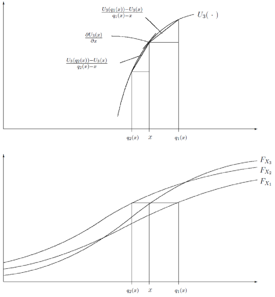
Figure 1: Bounds under the local curvature condition

The above argument works even if we do not know a priori whether $U_{T}(.)$ is concave or convex. Using the minimum and the maximum of the local discrete treatment effect will be sufficient to obtain bounds, provided that $U_{T}(.)$ is locally concave or locally convex around $x$. We therefore adopt the following definition.

Definition 1.

$x\mapsto U_{T}(x)$ is locally concave or convex on $[\widetilde{x},\widetilde{x}^{\prime}]$ if, almost surely (a.s.), it is twice differentiable and

$$\frac{\partial^{2}U_{T}}{\partial x^{2}}(x)\leq 0\;\forall x\in[\widetilde{x},\widetilde{x}^{\prime}]\;\text{a.s. or }\;\frac{\partial^{2}U_{T}}{\partial x^{2}}(x)\geq 0\;\forall x\in[\widetilde{x},\widetilde{x}^{\prime}]\;\text{a.s}.$$

Let us introduce, for all $(x,x^{\prime})\in\text{Supp}(X_{T})$, $(\underline{x}_{T}(x^{\prime}),\overline{x}_{T}(x^{\prime}))$ defined by

$$\underline{x}_{T}(x^{\prime}) = \max\{q_{t}(x),t\in\{1,...,T-1\}:\;q_{t}(x)\neq x\text{ and }q_{t}(x)<x^{\prime}\},$$

$$\overline{x}_{T}(x^{\prime}) = \min\{q_{t}(x),t\in\{1,...,T-1\}:\;q_{t}(x)\neq x\text{ and }q_{t}(x)>x^{\prime}\}.$$

If the sets are empty, we let $\underline{x}_{T}(x^{\prime})=-\infty$ and $\overline{x}_{T}(x^{\prime})=+\infty$.

Theorem 3.

Suppose that Assumptions 1-3 aresatisfied. For any $x<x^{\prime}$, if $U_{T}$ is locally concave or convex on $[\min(x,\underline{x}_{T}(x^{\prime})),\overline{x}_{T}(x^{\prime})]$, then

$$(x^{\prime}-x)\min\left\{\frac{\Delta^{ATT}(x,\underline{x}_{T}(x^{\prime}))}{\underline{x}_{T}(x^{\prime})-x},\frac{\Delta^{ATT}(x,\overline{x}_{T}(x^{\prime}))}{\overline{x}_{T}(x^{\prime})-x}\right\}\leq\Delta^{ATT}(x,x^{\prime})$$

$$\leq (x^{\prime}-x)\max\left\{\frac{\Delta^{ATT}(x,\underline{x}_{T}(x^{\prime}))}{\underline{x}_{T}(x^{\prime})-x},\frac{\Delta^{ATT}(x,\overline{x}_{T}(x^{\prime}))}{\overline{x}_{T}(x^{\prime})-x}\right\}.$$

If $U_{T}$ is locally concave or convex on $[\underline{x}_{T}(x),\overline{x}_{T}(x)]$, then

$$\min\left\{\frac{\Delta^{ATT}(x,\underline{x}_{T}(x))}{\underline{x}_{T}(x)-x},\frac{\Delta^{ATT}(x,\overline{x}_{T}(x))}{\overline{x}_{T}(x)-x}\right\}\leq\Delta^{AME}(x)$$

$$\leq \max\left\{\frac{\Delta^{ATT}(x,\underline{x}_{T}(x))}{\underline{x}_{T}(x)-x},\frac{\Delta^{ATT}(x,\overline{x}_{T}(x))}{\overline{x}_{T}(x)-x}\right\}.$$

The bounds are understood to be infinite when either $\underline{x}_{T}(x^{\prime})=-\infty$ or $\overline{x}_{T}(x^{\prime})=+\infty$ (whether $x^{\prime}>x$ or $x^{\prime}=x$).

Both bounds are finite, provided that there exists $t,t^{\prime}$ such that $q_{t}(x)<x<q_{t^{\prime}}(x)$, which implies that $T\geq 3$. More generally, the bounds improve with $T$, because $(\underline{x}_{T}(x^{\prime}))_{T\in\mathbb{N}}$ and $(\overline{x}_{T}(x^{\prime}))_{T\in\mathbb{N}}$ are by construction increasing and decreasing, respectively. Also, the local curvature condition becomes less restrictive as $T$ increases, because the interval on which $U_{T}$ has to satisfy this condition decreases. This condition is particularly credible if $q_{t}(x)\mapsto\Delta(x,q_{t}(x))/(q_{t}(x)-x)$ is monotonic, because such a pattern is implied by global concavity or global convexity.

Two other remarks on Theorem 3 are in order. First, we do not establish that the bounds are sharp, though we conjecture that they are. Second, similar to the point identification results of Theorem 1, the partial identification results of Theorem 3 can be extended to the multivariate setting. Specifically, we can use the system of inequalities

$$U_{T}(q_{t}(x))-U_{t}(x)\geq\frac{\partial U_{T}(x)}{\partial x}^{\prime}(q_{t}(x)-x),$$

which hold for all $t=1...T-1$ if $U_{T}$ is locally convex (inequalities are reverted if $U_{T}$ is locally concave). These inequalities imply some bounds on $E[\partial U_{T}(x)/\partial x]$. A necessary condition for the bounds to be finite on each component of $E[\partial U_{T}(x)/\partial x]$ is that $T-1\geq 2\dim(X_{t})$. This condition generalizes the above restriction $T\geq 3$. It makes intuitive sense that more time periods are required when the endogenous treatment is multivariate.

To illustrate Theorem 3, we consider the following example:

$$Y_{t} = 1-\exp(-0.5(\delta_{t}+X_{t}+U_{t}))$$

$$X_{t} = \mu_{t}+\sigma_{t}\Phi^{-1}(V_{t}),$$

where $V_{t}\sim U[0,1]$ and $U_{t}|V_{t}\sim\mathcal{N}(V_{t},1)$. We also suppose that

$$\mu_{T}=2.5, \mu_{t}\sim\mathcal{N}(\mu_{T},1)\;\text{for }t<T,$$

$$\sigma_{T}=1, \sigma_{t}\sim\chi^{2}(1)\;\text{for }t<T,$$

$$\delta_{T}=0, \delta_{t}\sim\mathcal{N}(0,1)\;\text{for }t<T.$$

In this example, Assumptions 1, 2 (with $g_{t}(y)=1-\exp(-0.5\delta_{t})(1-y)$) and 3 are satisfied, the latter because $\sigma_{t}\neq\sigma_{T}$ almost surely. The local curvature condition also holds, since $u\mapsto 1-\exp(-0.5u)$ is concave. Figure 2 displays the bounds on $\Delta_{1}^{AME}(x)$ for $T=3,4,5$ and 6. Note that the bounds coincide for $T-1$ points. This simply reflects the point identification result of Theorem 6. We also see that in the interval where we get finite bounds, i.e., the interval for which $-\infty<\underline{x}_{T}(x)<\overline{x}_{T}(x)<\infty$, the bounds are quite informative even for $T=3$. Figure 2 also shows that as $T$ increases, both the bounds shrink and the interval on which we get finite bounds increase. For $T=6$, we get informative bounds for $x\in[1,\;3.85]$, which corresponds roughly to 85% of the population. This means that we could also obtain finite bounds for the average partial effect for this large fraction of the total population.

$T=3$

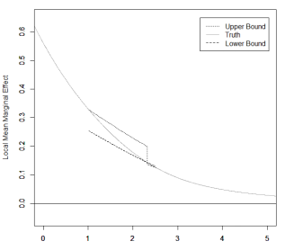
$T=4$

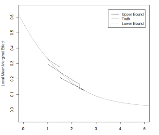
$T=5$

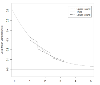
$T=6$

Figure 2: Example of bounds on $\Delta^{AME}(x)$ for different values of $x$ and $T=3,4,5$ and $6$.

3.4 Point Identification with a Correlated Random Coefficient Model

As we have established in Theorem 1, we can point identify several treatment effect parameters under Assumptions 1-3, but these are by no means all possible causal effects one may be interested in. Many more treatment parameters can be set identified under often plausible curvature restrictions, in particular average marginal effects and effects of the kind $\Delta^{ATT}(x,x^{\prime})$. However, these bounds may be wide in some applications, conducting inference on the corresponding parameters may be cumbersome or even impractical. Hence it makes sense to search for additional assumptions that yield point identification of average structural effects over the entire population.

We suggest here a possible route for extrapolation, based on a random coefficient linear model of the form:

$$Y_{t}(x)=\delta_{t}+U_{0t}+xU_{1t}.$$ (3.1)

Therefore, we impose a linear structure on $g_{t}$ ($g_{t}(u)=\delta_{t}+u$ and $U_{t}(x)$ ($U_{t}(x)=U_{0t}+xU_{1t}$). The model still allows for a rich, non-scalar heterogeneity pattern through the two unobserved terms $U_{0t}$ and $U_{1t}$. Under this structure, we have, for any $(x,x^{\prime})\in\text{Supp}(X_{T})^{2}$, $x\neq x^{\prime}$,

$$\frac{\Delta^{ATT}(x,q_{t}(x))}{q_{t}(x)-x}=E\left[U_{1T}|X_{T}=x\right]=\Delta^{AME}(x)=\frac{\Delta^{ATT}(x,x^{\prime})}{x^{\prime}-x}.$$ (3.2)

By Theorem 1, $\Delta^{ATT}(x,q_{t}(x))$ is point identified under Assumptions 1-4. This implies that $\Delta^{AME}(x)$ and $\Delta^{ATT}(x,x^{\prime})$ are identified as well, whenever $q_{t}(x)\neq x$. As a result, the average marginal effect over the whole population, $\Delta^{AME}=E\left[\Delta^{AME}(X_{T})\right]$, is also point identified if $q_{t}(X_{T})\neq X_{T}$ almost surely. We summarize this finding in the following theorem.

Theorem 4.

Under Assumptions 1-4 and Equation (3.1), for all $t<T$ and $(x,x^{\prime})\in\text{Supp}(X_{T})^{2}$, $q_{t}(x)\neq x$, $(\delta_{t})_{t<T}$, $\Delta^{ATT}(x,x^{\prime})$ and $\Delta^{AME}(x)$ are identified. If $q_{t}(X_{T})\neq X_{T}$ almost surely, $\Delta^{AME}$ is point identified as well.

Several remarks on this result are in order. First, we recover the same parameter as Graham and Powell (2012), who also consider a random coefficient linear model similar to (3.1). They obtain identification with panel data, relying on first-differencing. Compared to them, we rely on variations in the cdf of $X_{t}$ rather than on individual variations. We rely on a different, non-nested, restriction on the distribution of the error term. In particular, for the same individual, $U_{1t}-U_{1s}$ could be correlated with $X_{t}$ in our framework.

Second, Theorem 4 readily extends to a multivariate treatment, by just replacing the condition $q_{t}(x)\neq x$ by a rank condition. Specifically, let, as in Section 3.2, $q_{t}(x)=(q_{1t}(x_{1}),...,q_{kt}(x_{k}))^{\prime}$ and define the matrix $\mathbf{Q}(x)$ by

$$\mathbf{Q}(x)=\left[\begin{array}[]{c}(q_{1}(x)-x)^{\prime}\\ \vdots\\ (q_{T-1}(x)-x)^{\prime}\end{array}\right].$$

Then $\Delta^{AME}(x)$ and $\Delta^{ATT}(x,x^{\prime})$ are identified if $\mathbf{Q}(x)$ is full column rank. Note that the rank condition implies that $T-1\geq k$. It also implies that the distribution of $X_{t}$ differs at each date, so that $q_{s}(x)\neq q_{t}(x)$. It makes sense that with several endogenous variables, more time variation on $X_{t}$ is needed to identify causal effects.

Third, coming back to the univariate case, Theorem 4 ensures that all parameters of interest are identified with only two time periods. This suggests that the model can be either tested or enriched when $T>2$. To see why the linearity assumption is testable when $T>2$, note that Equation (3.2) implies

$$\frac{\Delta^{ATT}(x,q_{s}(x))}{q_{s}(x)-x}=\frac{\Delta^{ATT}(x,q_{t}(x))}{q_{t}(x)-x}\quad\forall s\neq t,$$

which can be checked in the data. With more than two time periods, we can also identify treatment effects in the more general random coefficient polynomial model of order $T-1$:

$$Y_{t}=\delta_{t}+U_{0t}+U_{1t}X_{t}+...+U_{T-1t}X_{t}^{T-1}.$$ (3.3)

With the same arguments as above, we recover not only average marginal effect, but actually $E(U_{kt}|X_{t}=x)$ for all $k=1,...,T$ and all $x$ such that $(x,q_{1}(x),...,q_{T-1}(x))$ are all distinct. Identification of a model similar to (3.3) was studied before by Florens et al. (2008), with cross-sectional data and under assumptions that typically rule out discrete instruments (see also Heckman and Vytlacil, 1998, for a study of the identification of Model (3.1) with instruments). Here, we rely only on a finite number of time periods, which would be equivalent to a discrete instrument, and allow for time trend, which would correspond to a direct effect of the instrument in Florens et al. (2008).

Alternatively, we can use additional periods to identify higher moments of the distribution of the coefficients in the linear model (3.1). For instance, with $k=1$, $V(U_{01}|X_{T}=x)$, $V(U_{1T}|X_{T}=x)$ and Cov$(U_{01},U_{1T}|X_{T}=x)$ can be shown to be identified with $T=3$ as soon as $x,q_{1}(x)$ and $q_{2}(x)$ are distinct.

4 Estimation of Average and Quantile Treatment Effects

We consider in this section estimators of the parameters $\Delta^{ATT}(x,q_{t}(x))$ and $\Delta^{QTT}(p,x,q_{t}(x))$ that are shown to be identified in Theorem 1. We suppose for that purpose to observe two independent samples corresponding to the periods $1$ and $T=2$. For simplicity, we suppose hereafter that the two corresponding sample sizes are identical.

Assumption 5.

We observe the two independent samples $(Y_{i1},X_{i1})_{i=1...n}$ and $(Y_{i2},X_{i2})_{i=1...n}$, which are both i.i.d. random variables drawn from the distributions $F_{Y_{1},X_{1}}$ and $F_{Y_{2},X_{2}}$, respectively.

Our estimator follows closely our identification strategy. Let us define

$$\Psi_{n}(x)=\widehat{F}_{X_{2}}(x)-\widehat{F}_{X_{1}}(x),$$

where $\widehat{F}_{X_{2}}$ (resp. $\widehat{F}_{X_{1}}$ ) denotes the empirical cdf of $X_{2}$ (resp. $X_{1}$). We first estimate $x^{*}_{1}$ by

$$\widehat{x}^{\ast}_{1}=\min\left\{x\in\left[\widehat{F}_{X_{1}}^{-1}(\underline{p}),\widehat{F}_{X_{1}}^{-1}(\overline{p})\right]:\,|\Psi_{n}(x)|\leq|\Psi_{n}(x^{\prime})|\;\forall x^{\prime}\in\left[\widehat{F}_{X_{1}}^{-1}(\underline{p}),\widehat{F}_{X_{1}}^{-1}(\overline{p})\right]\right\},$$ (4.1)

where $\widehat{F}_{X_{1}}^{-1}$ denotes the empirical quantile function and $0<\underline{p}<\overline{p}<1$ are two given constants used to avoid reaching the boundaries of the support of $X_{1}$. Note that the minimum in (4.1) is well defined because $\Psi_{n}$ is a right-continuous step function.

Next, we estimate $q_{1}(x)=F_{X_{1}}^{-1}\circ F_{X_{2}}(x)$ by its empirical counterpart $\widehat{q}_{1}(x)=\widehat{F}_{X_{1}}^{-1}\circ\widehat{F}_{X_{2}}(x)$. We then estimate $g_{1}$ using an empirical counterpart of (2.5). For that purpose, we estimate the conditional cdf $F_{Y_{t}|X_{t}}$, for $t\in\{1,2\}$, by

$$\widehat{F}_{Y_{t}|X_{t}}(y|x)=\frac{\sum_{i=1}^{n}\mathds{1}\{Y_{it}\leq y\}K\left(\frac{x-X_{it}}{h_{n}}\right)}{\sum_{i=1}^{n}K\left(\frac{x-X_{it}}{h_{n}}\right)},$$

where $K$ is a kernel function and $h_{n}$ denotes the bandwidth. We then let $\widehat{F}_{Y_{t}|X_{t}}^{-1}(.|x)$ denote the generalized inverse of $\widehat{F}_{Y_{t}|X_{t}}(.|x)$. We estimate $g_{1}$ by

$$\widehat{g}_{1}(y)=\widehat{F}_{Y_{1}|X_{1}}^{-1}\left[\widehat{F}_{Y_{2}|X_{2}}(y|\widehat{x}_{1}^{\ast})|\widehat{x}_{1}^{\ast}\right].$$

Now, let us recall that $\Delta^{ATT}(x,q_{1}(x))$ and $\Delta^{QTT}(p,x,q_{1}(x))$ satisfy, under Assumptions 1-3,

$$\Delta^{ATT}(x,q_{1}(x)) =E[g_{1}(Y_{1})|X_{1}=q_{1}(x)]-E[Y_{2}|X_{2}=x],$$

$$\Delta^{QTT}(p,x,q_{1}(x)) =F_{g_{1}(Y_{1})|X_{1}}^{-1}(p|q_{1}(x))-F_{Y_{2}|X_{2}}^{-1}(p|x).$$

We then estimate these two parameters by

$$\widehat{\Delta}^{ATT}(x,q_{1}(x)) =\frac{\sum_{i=1}^{n}\widehat{g}_{1}^{-1}(Y_{i1})K\left(\frac{x-X_{i1}}{h_{n}}\right)}{\sum_{i=1}^{n}K\left(\frac{x-X_{i1}}{h_{n}}\right)}-\frac{\sum_{i=1}^{n}Y_{i2}K\left(\frac{x-X_{i2}}{h_{n}}\right)}{\sum_{i=1}^{n}K\left(\frac{x-X_{i2}}{h_{n}}\right)}\qquad\text{and}$$

$$\widehat{\Delta}^{QTT}(p,x,q_{1}(x)) =\widehat{F}_{\widehat{g}_{1}(Y_{1})|X_{1}}^{-1}(p|\widehat{q}_{1}(x))-\widehat{F}_{Y_{2}|X_{2}}^{-1}(p|x).$$

For notational simplicity, we chose here the same kernels and bandwidths for each nonparametric terms, though we could obviously consider different ones. We establish below that $\widehat{\Delta}^{ATT}(x,q_{1}(x))$ and $\widehat{\Delta}^{QTT}(p,x,q_{1}(x))$ are consistent and asymptotically normal. Our result is based on the following conditions.

Assumption 6.

(Conditions for the root-n consistency of $\widehat{x}^{\ast}_{1}$ and $\widehat{q}_{1}(x)$)
(i) There exists a unique $x^{*}_{1}$ satisfying $F_{X_{1}}(x^{*}_{1})=F_{X_{2}}(x^{*}_{1})\in(0,1)$. Moreover, $F_{X_{1}}(x^{*}_{1})\in(\underline{p},\overline{p})$.
(ii) For $t\in\{1,2\}$, $X_{t}$ admits a continuous density $f_{X_{t}}$ satisfying, for all $x$ in the interior of $\mathcal{X}$, $f_{X_{t}}(x)>0$. Moreover, $f_{X_{1}}(x^{*}_{1})\neq f_{X_{2}}(x^{*}_{1})$.

Assumption 7.

(Regularity conditions on $(X_{t},Y_{t})$)
(i) For $t\in\{1,2\}$, $\text{Supp}(X_{t},Y_{t})=\mathcal{X}\times\mathcal{Y}$ with $\mathcal{Y}=[\underline{y},\overline{y}]$ with $-\infty<\underline{y}<\overline{y}<+\infty$.
(ii) For $(t,x)\in\{1,2\}\times\mathcal{X}$, $F_{Y_{t}|X_{t}}(.|.)$ is continuously differentiable and $\inf_{y\in\mathcal{Y}}f_{Y_{t}|X_{t}}(y|x)>0$.
(iii) For all $(t,y)\in\{1,2\}\times\mathcal{Y}$, $F_{Y_{t}|X_{t}}(y|.)$ and $f_{X_{t}}$ are twice differentiable. $f_{X_{t}}$, $|f^{\prime}_{X_{t}}|$ and $|f^{\prime\prime}_{X_{t}}|$ are bounded. $\sup_{(y,x)\in\mathcal{Y}\times\mathcal{X}}|\partial_{x}F_{Y_{t}|X_{t}}(y|x)|<\infty$ and $\sup_{(y,x)\in\mathcal{Y}\times\mathcal{X}}|\partial_{xx}F_{Y_{t}|X_{t}}(y|x)|<\infty$.

Assumption 8.

(Conditions on the kernels and bandwidths)
(i) $nh^{3}_{n}/|\log(h_{n})|\rightarrow+\infty$, $nh_{n}^{5}\rightarrow 0$.
(ii) $K$ has a compact support, is differentiable with $K^{\prime}$ of bounded variation and satisfies $K(y)\geq 0$ for all $y$. Besides, $\int K(y)dy=1$ and $\int yK(y)dy=0$.

Assumption 6-(i) strengthens Assumption 3 by assuming the uniqueness of the crossing point. We make this assumption for the sake of simplicity. We could also consider the case where the set of crossing points is an interval. As discussed in Section 2.3.1 above, we would actually expect a parametric rather than a nonparametric rate of convergence for $\widehat{g}_{1}$, so Theorem 5 below should still hold in this more favorable case. Assumption 6-(ii) is a mild regularity condition on $F_{X_{2}}$ and $F_{X_{1}}$. As Lemmas 2 and 4 in Appendix A show, these two restrictions ensure that $\widehat{x}_{1}^{\ast}$ and $\widehat{q}_{1}(x)$ are root-n consistent. Assumption 7 provides a set of conditions ensuring that $\widehat{g}_{1}$ is consistent and asymptotically normal. Conditions (i) and (ii) are also made by Athey and Imbens (2006), without any $X_{t}$ in their case, in another context where quantile-quantile transforms must be estimated. Condition (iii) is required as well here because we deal with nonparametric estimators of conditional cdfs rather than usual empirical cdfs, as Athey and Imbens (2006) do. Finally, Assumption 8 is a standard condition on the bandwidths and the kernels appearing in the nonparametric estimators. We impose $nh_{n}^{5}\rightarrow 0$ in order to avoid any asymptotic bias on $\widehat{\Delta}^{ATT}(x,q_{1}(x))$ and $\widehat{\Delta}^{QTT}(p,x,q_{1}(x))$.

Theorem 5.

Suppose that Assumptions 1-4 and 5-8 are satisfied. Then, for any $x\in\mathcal{X}$ such that $F_{X_{1}}$ is differentiable at $q_{1}(x)$ with $F_{X_{1}}^{\prime}(q_{1}(x))>0$,

$$\sqrt{nh_{n}}\left(\widehat{\Delta}^{ATT}(x,q_{1}(x))-\Delta^{ATT}(x,q_{1}(x))\right) \overset{d}{\longrightarrow}\mathcal{N}(0,V_{1})$$

$$\sqrt{nh_{n}}\left(\widehat{\Delta}^{QTT}(p,x,q_{1}(x))-\Delta^{QTT}(p,x,q_{1}(x))\right) \overset{d}{\longrightarrow}\mathcal{N}(0,V_{2}),$$

for some $V_{1},V_{2}$.

We do not display the asymptotic variances here, as they involve many terms due to the multiple compositions of nonparametric estimators – see Appendix B.3 for details as well as a proof. In practice, we suggest to rely on bootstrap, as we do in the application below. We conjecture that the bootstrap is consistent in our setting, though a formal proof of its validity is beyond the scope of this paper. The main issue for establishing its validity would be to prove the (conditional) weak convergence of the process

$$G_{nxt}^{*}=\sqrt{nh_{n}}\left(\widehat{F}^{*}_{Y_{t}|X_{t}}(.|x)-\widehat{F}_{Y_{t}|X_{t}}(.|x)\right),\;t\in\{1,2\},$$

where $\widehat{F}^{*}_{Y_{t}|X_{t}}$ is the bootstrap counterpart of $\widehat{F}_{Y_{t}|X_{t}}$. Up to our knowledge, such a result is not available in the literature yet.

5 Application to the Marginal Propensity to Consume

In this section we provide an application to a substantive economic question: The magnitude of the marginal propensity to consume out of current disposable income. When analyzing this question, we focus in particular on how results obtained through our approach compare to those obtained in the literature. In order to facilitate this comparison, we first briefly review the literature on this question, before explaining the policy experiment we are using, and detailing the data. We then outline how our methodology is employed, and finally close by comparing our results with those in the literature.

5.1 The Economic Question

A crucial question for the classical theory of consumption is the marginal propensity to consume (MPC) out of income. Given its implications for the business cycle, taxes, and government policy, the importance of the MPC can hardly be overstated, and thus this quantity was, and still is, at the center of a very active debate (see, e.g., Jappelli and Pistaferri, 2010, for an overview). An upshot of the rational expectations revolution which, since the seminal paper of Hall (1978), tried to answer questions about the effect of a marginal change in income on consumption, is that expectations about the change matter.

In the absence of liquidity constraints (and precautionary saving motives at very low income levels), the following is the key insight in the literature about the effect of a marginal income change on the nondurable consumption of a rational consumer, see, e.g., Deaton (1992): If the income change is anticipated, i.e., not related to new information, then consumption does not respond to the income change. For an income change that is not anticipated, if the change is viewed as transitory, then the rational consumer is predicted to use very little of the income increase immediately, as the transitory change in income is distributed over the life-cycle, and its small quantity (relative to life-cycle income) does not alter fundamentally the trade-off between consumption today and saving for the future. Conversely, if the income change is expected to be permanent, the individual is expected to essentially increase her consumption by the amount of the change. This means that we only observe a substantial change in consumption in response to an income change, if the change is surprising and considered to be permanent.

The empirical evidence on the hypothesis of a rational consumer is rather mixed, and has spurned an active debate. Perhaps the most problematic evidence comes from studies involving one time transfers, see e.g., Johnson et al. (2006) and Parker et al. (2013, PSJM). In these studies, consumers are given what is clearly an expected and transitory income shock (PSJM actually documenting aspects of the Obama era stimulus package), yet the effect on consumption is not zero. Instead, typical estimates for the marginal effects of an anticipated income change range between 15% and 25%.

There are a number of counterarguments in defense of the rational consumer. First, consumers could be credit constrained. PSJM find indeed lower responses for older and high-income households, who are less likely to be constrained. Second, consumers may exhibit a form of bounded rationality. There are significant costs associated with computing the optimal consumption path. If an income change is small relative to the level of income, the benefits from adapting the optimal path in light of the changes are small relatively to the costs associated with it, and individuals simply avoid optimizing completely, as they would in the case of a large income change. Evidence that individuals indeed smooth large anticipated income changes is provided by Browning and Collado (2001) and Hsieh (2003), among others. Another counterargument is that some of the changes considered in the literature are not just small, but also outside the “usual” consumer experience. As such, they are not representative of the typical real-world surprise income shocks individuals deal with (a distinction that is reminiscent to the question of whether individuals are able to assign probabilities to these events).

In this section, we use our econometric method in conjunction with an experiment involving the Earned Income Tax Credit (EITC) to analyze the causal effect of increase in income on consumption for households in 1987. We believe that this natural experiment is very insightful for the above debate. While it provides exactly the type of variation we require for our method, it provides (at least for a good number of households) a significant and anticipated change in their income. Finally, the fact that our procedure allows for nonlinearities, i.e., for the marginal effect to vary with income, is going to be crucial to shed light on the question of the existence of liquidity constraints.

5.2 Policy Background: The EITC

In the following, we provide more background on the policy experiment that provides the exogenous variation: The Earned Income Tax Credit (EITC) is an income support program which started in 1975 in the United States for the purpose of mitigating poverty. The EITC provision schedule varies from year to year, exhibiting interesting non-linearities. This feature of the program has been used for economic analysis before, e.g., by Dahl and Lochner (2012), and a detailed documentation of the EITC can be found in Falk (2014). In most of the past years, the change to the EITC schedule has been monotone to match increasing price levels. However, the change in the schedules between 1987 and 1989 exhibits a specific pattern which, as we will now demonstrate, generates a crossing of the cdfs of (deflated) total income in the respective years.

Figure 3 displays the EITC schedules in 1987 (solid line) and 1989 (dotted line) in terms of thousands of Year 2000 US dollars for families with two or more children. Note that for individuals with income between 9K USD and 10.75K USD, the 1987 EITC provision was higher than the provision in 1989, whereas the reverse is true for individuals with income above 10.75K USD. This is exactly the type of variation which generates a crossing, if everything else is held constant.

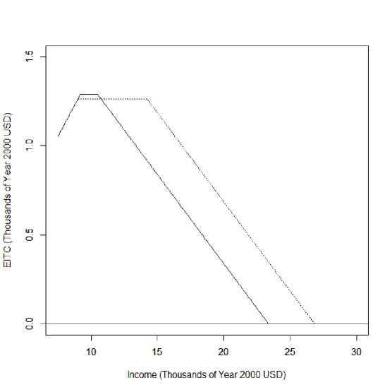
Notes: amount of the EITC in 1987 (solid line) and 1989 (dotted line), for families with two or more children.

Figure 3: EITC schedules in 1987 and 1989

To see this more precisely, consider the left graph in Figure 4. The graph shows total income, obtained as the sum of the pre-aid income and the EITC amount, for each of the years 1987 (solid line) and 1989 (dotted line) plotted against that of year 1989, i.e., the solid line is the 45-degree line. The right graph in the same figure (Fig. 4) focuses on this difference. As these figures suggest, we expect a crossing at 12K USD, computed as the sum of 10.75K USD (the cut-off for the change in the schedule) and 1.25K USD for the corresponding EITC amount, provided that total pre-EITC income does not change substantially. Note that these figures are solely derived from the known policy schedules, but we will confirm our expectation with real data below. Before we detail this, however, we first give an overview of the data.

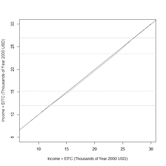
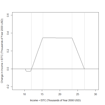
Notes: left panel: total income, obtained as the sum of the pre-aid income and the EITC amount, for 1987 and 1989 plotted against that of 1989. Right panel: the change in the total income, obtained as the sum of the pre-aid income and the EITC amount, between 1987 and 1989.

Figure 4: Theoretical change in total disposable income between 1987 and 1989 due to EITC change.

5.3 Data: The CEX

For our analysis, we use repeated cross-sectional data from the Consumer Expenditure Survey (CEX) for the calendar years 1987 and 1989. The treatment variable is, more precisely, total disposable family income measured in thousands of Year 2000 US dollars. The outcome (dependent) variable is non-durable household consumption, defined as the sum of expenditures for food at home, apparel, health, entertainment, personal care, and readings, measured in thousands of Year 2000 US dollars. Since the policy described above applies only to families with two or more children, we use the sub-sample of individuals with two or more children. Table 1 shows summary statistics for our sub-sample.

Note that after controlling for inflation (i.e., in year 2000 prices), the mean of total family disposable income does not change substantially between 1987 and 1989 (roughly 2%). Indeed, this modest increase from 1987 to 1989 is quite consistent with the EITC policy change and an otherwise pretty stationary environment, strengthening the case that we should expect to have the type of variation in cdfs our method requires.

	Thousands of present year USD			Thousands of Year 2000 USD
Whole Sample	1987	1989		1987	1989
Total Family Income	27.973	31.162		42.402	43.275
	(20.944)	(23.438)		(31.747)	(32.548)
CEX Nondurable Consumption	9.072	10.787		13.752	14.980
	(6.187)	(8.872)		(9.378)	(12.320)
Number of Observations	4,827	4,120		4,827	4,120
Subsample: Total Disposable	Thousands of present year USD			Thousands of Year 2000 USD
Family Income $\in[15.2,23.4]$	1987	1989		1987	1989
CEX Nondurable Consumption	6.132	7.426		9.296	10.312
	(3.606)	(5.655)		(5.467)	7.854
Consumption/Income Ratio	0.491	0.536		0.491	0.536
	(0.289)	(0.386)		(0.289)	(0.386)
Number of Observations	559	442		559	442
Notes: CEX data restricted to famiies with two or more children for 1987 and 1989. The standard deviations are indicated in parentheses.

Table 1: Relevant Summary Statistics of the CEX Data

Turning to our nondurable consumption measure, we first notice that it only captures a little less than half of disposable income. Within the subsample that we focus on, the average ratio of nondurable consumption to total disposable income (which is different than the ratio of averages) is around 50%. This may be due to the fact that the large category of rent and mortgage payments are excluded as are large and durable and nondurable consumption items (e.g., TVs, cars, phones). However, we also suspect a certain modest degree of underreporting in the data. Like in the standard Diff-in-Diff approach, our analysis would be invalidated if the evolution of this underreporting is systematically different between treatment and control group. We believe this to be unlikely and certainly have no evidence of this difference in effects. Moreover, since the overall degree of underreporting seems to be tolerable as well (e.g., food and clothing account for a budget share of 50% in the British FES as well, see Hoderlein (2011)), we hence proceed with our analysis.

One thing that stands out is that the nondurable consumption measure increased more than proportionally to the change in disposable income in both the sample we focus on (average share increase from 49.1% to 53.6%), but also in the population at large. This may be due to changes in economic outlook and general optimism in 1989 at the end of the cold war. Because of this observation, we definitely want to include a time trend $g_{t}$ in the empirical analysis, as our method warrants. Indeed, our model identifies an increase in nondurable consumption in particular at higher levels of the consumption distribution even if our policy experiment would not have taken place.

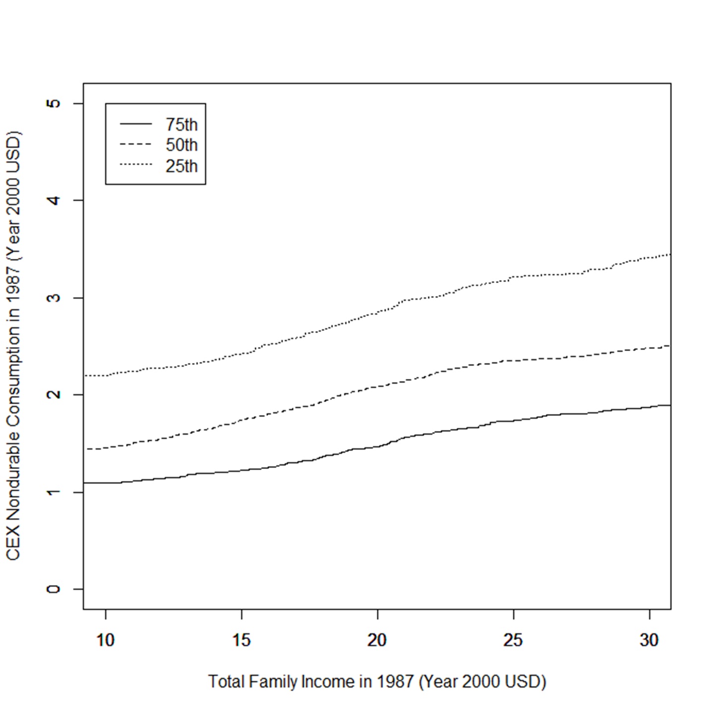
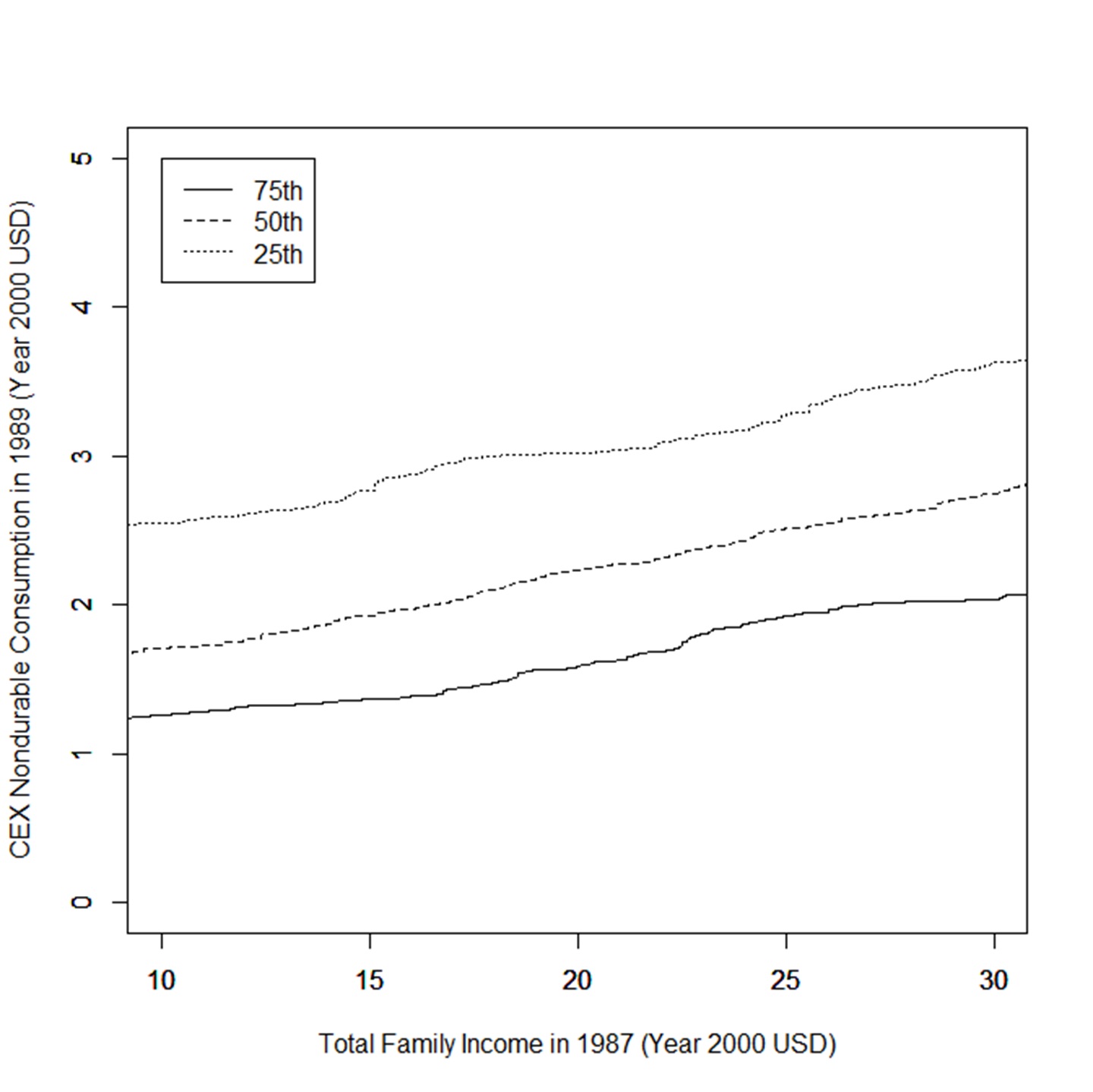
Notes: CEX data restricted to families with two or more children. Family income is given in thousands of 2000 US dollars.

Figure 5: Conditional quartiles of $Y_{t}$ (CEX nondurable consumption) given $X_{t}$ (total family income) in 1987 and 1989

5.4 Analysis and Results

First, we use our data to confirm that the policy change in the EITC described above indeed induces a crossing in the cdfs. In particular, we want to study whether there is a divergence from 12.0 K to 26.8 K USD of cdfs of total family income between 1987 and 1989. The left panel of Figure 6 displays the two empirical cdfs. The solid vertical lines indicate the limit points of the range inside which the policy change matters; these lines correspond to those displayed in Figure 4. To check that the distributions of income are in line with this policy change, we made one-sided test of $F_{1}(x)\leq F_{2}(x)$ for all $x\in[12.0K,26.8K]$. We find that at the 5% level, $F_{1}(x)>F_{2}(x)$ for at least some $x\in[12.0K,26.8K]$. We take this as strong evidence that the change in the EITC was, at least for this subpopulation of households, the main driving force in the change of the empirical cdfs between the two years. Moreover, the direction of the crossing is what we expect from the design of the policy change: the families falling within the range where we expect an increase in total disposable income due to the change in EITC experience a positive change in total family income between 1987 to 1989.

Using these two empirical cdfs, we next compute the empirical quantile-quantile plot of the total family income from 1987 to 1989 in terms of Year 2000 US dollars. The right panel of Figure 6 displays the plot. Observe how well this data-based figure resembles Figure 4, which is constructed using the policy formulas. This provides further evidence that the data follows our research design, and that there are no other major unaccounted sources of change in disposable income. Recall, moreover, that this quantile-quantile plot, which is mathematically represented by $q_{1}$ in our framework, is the main building block for our identification results.

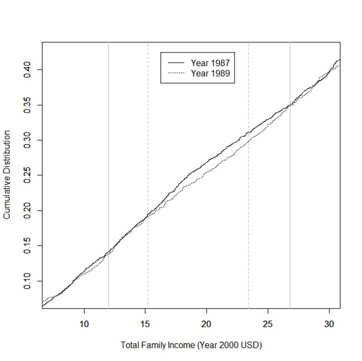
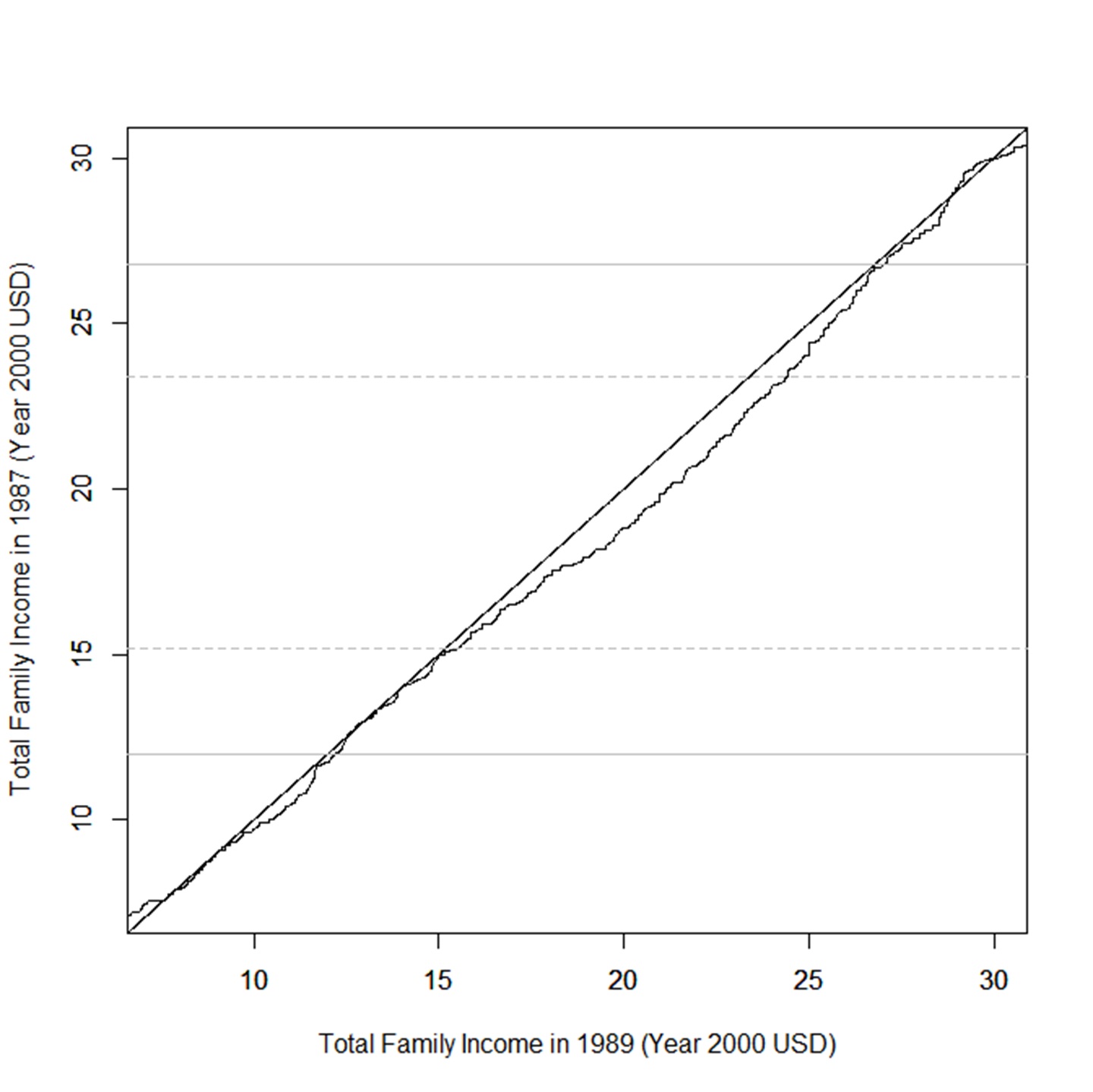
Notes: CEX data restricted to families with two or more children. Family income is given in thousands of 2000 US dollars. In the left panel, the black (resp. grey) curve corresponds to family income in 1987 (resp. 1989). In the right panel, we display the Q-Q plot, i.e. $q_{1}$ against the identity function. The solid lines indicate the theoretical limits inside which we should observe a divergence of the cdfs, given the policy design. The dotted lines are the limits of the interval on which the efffect of the policy is supposed to be maximal (see the right panel of Figure 4).

Figure 6: Cdf’s and Q-Q plot of total family income in 1987 and 1989

After having confirmed that the change in the distribution of the treatment is in line with our modeling assumption and largely driven by the policy change, we proceed to use our framework and estimate the time trend $g_{1}(.)$. In line with the theoretical design, Figure 6 shows that we have more than a single point $x^{\ast}$ as a control group. We can use the whole set $\mathcal{S}=[10K;12K]\cup[26,8K;50K]$, where the two cdfs overlay. This results in more precise estimates of $g_{1}(.)$ and marginal effects, because we can use the whole set $\mathcal{S}$ instead of a single point $x^{\ast}$. Specifically, we can use $g_{1}(y)=F_{Y_{1}|X_{1}\in\mathcal{S}}^{-1}\left[F_{Y_{2}|X_{2}\in\mathcal{S}}(y)\right]$ instead of $g_{1}(y)=F_{Y_{1}|X_{1}}^{-1}\left[F_{Y_{2}|X_{2}}(y|x^{\ast})|x^{\ast}\right]$. Figure 7 displays the estimate of $g_{1}^{-1}$, which corresponds to the (heterogeneous) time trend between 1987 and 1989. As mentioned before, we observe an increase in the upper tail of the distribution of nondurable consumption, corresponding with an improved overall economic outlook, in particular for middle and upper class households.

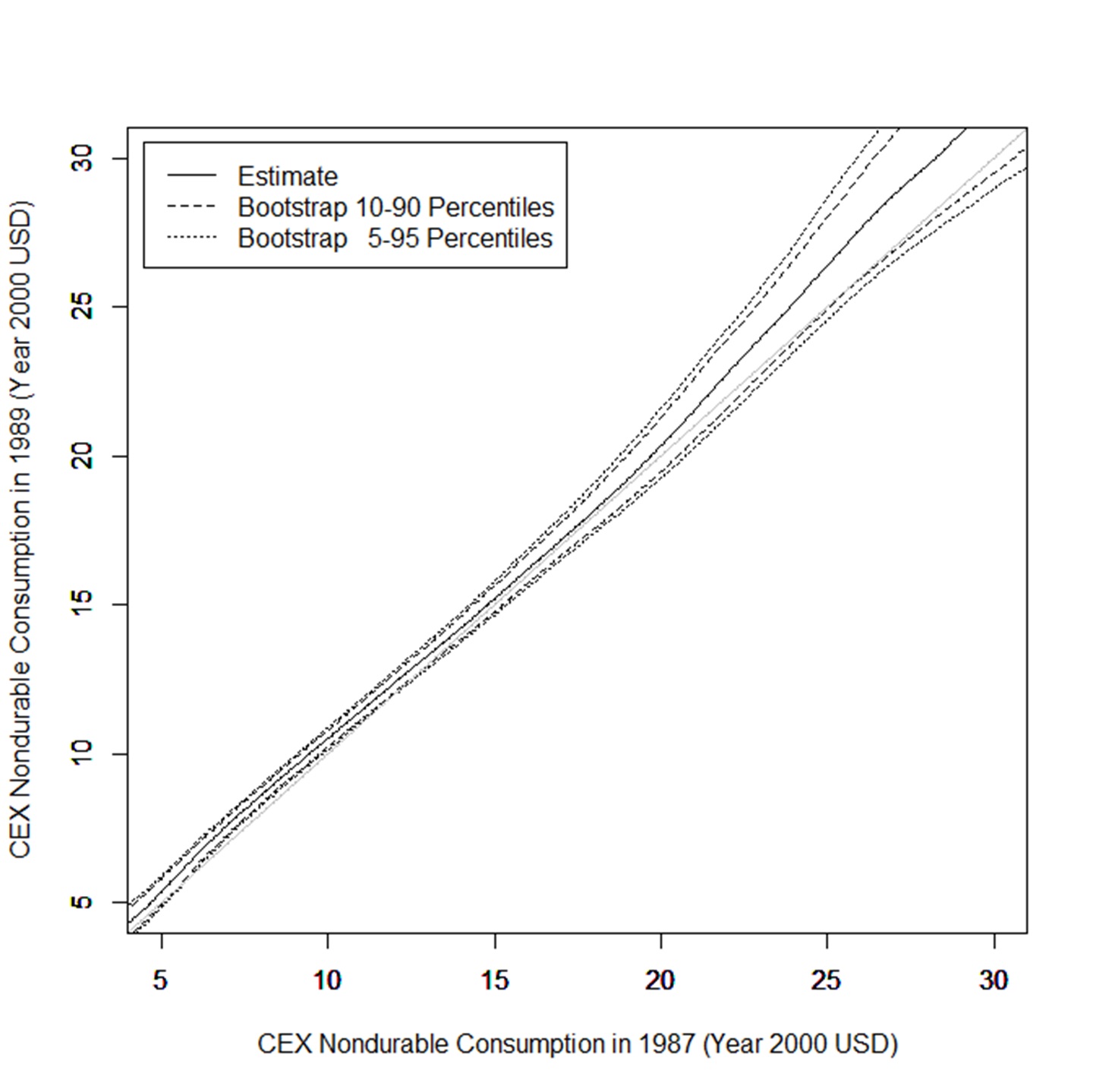
Notes: CEX data restricted to families with two or more children. Curves are kernel-smoothed. CEX nondurable consumptions are in thousands of year 2000 US dollars.

Figure 7: Estimate of the time trend function $g_{1}^{-1}$ from 1987 to 1989.

To come to the main purpose of this application, we estimate average marginal effects of the total family income in 1987 in terms of Year 2000 US dollars on various expenditures in terms of Year 2000 US dollars. Specifically, we estimate $\Delta_{app}^{AME}(x)=\Delta^{ATT}(x,q_{1}(x))/(q_{1}(x)-x)$ instead of $\Delta^{ATT}(x,q_{1}(x))$. The former quantity has the advantage over the latter of being interpretable as an average marginal effect. By the mean value theorem (and under mild regularity conditions), indeed, $\Delta_{app}^{AME}(x)=E\left[dY_{2}/dx(\widetilde{X})|X_{2}=x\right]$, for some random $\widetilde{X}\in[q_{1}(x),x]$. To the extent that $q_{1}(x)$ is close to $x$, we then interpret $\Delta_{app}^{AME}(x)$ as the average marginal effect at $X_{2}=x$. Note, on the other hand, that by dividing by $\widehat{q}_{1}(x)-x$, the estimator of $\Delta_{app}^{AME}(x)$ is more volatile than that of $\Delta^{ATT}(x,q_{1}(x))$, especially when $q_{1}(x)-x$ is close to zero. To obtain more precise estimates, we rely hereafter on a piecewise linear estimator of $q_{1}(x)-x$. Such a constrained estimator is consistent with the policy design and fits well the data. We refer to Appendix C for more details on its construction.

Figure 8 presents the estimated average marginal effects. The estimates are displayed on the interval $[15.2,23.8]$, namely the interval on which the EITC policy change is supposed to be pronounced. We focus on this region because elsewhere the denominator of $\Delta_{app}^{AME}(x)$ is either close or equal to zero. The solid line represents the point estimate of the average marginal effect. Specifically, the line shows how much out of one dollar increase is spent on our nondurable consumption bundle. Our results are very much in line with the literature, with values ranging from 0.5 for disposable income just below $16K to virtually zero for incomes above $22K. Our point estimate also suggests that the average marginal effect decreases with income. This is in line with previous findings in the literature, in particular those of PSJM. Such a pattern is also consistent with rational consumers facing credit constraints. Indeed, credit constraints are likely to be less severe for households with higher income, as such consumers are on average more able to use parts of their wealth as collateral to get new credits more easily.

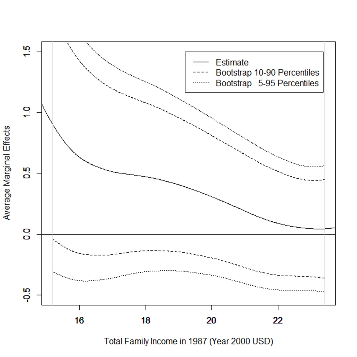
Notes: CEX data restricted to families with two or more children. Curves are kernel-smoothed. Income and consumption are in thousands of 2000 USD. The vertical lines indicate the limits of the region with cdf divergence.

Figure 8: Average marginal effects of total family income on CEX nondurable consumption

Several remarks are in order. The first concerns significance: While the results for low levels of disposable income are borderline pointwise significant at the 90% level, most of the estimated effect is insignificant (as are results based on 95% significance). This is in particular regrettable at income levels around $ 18K where there is probably a substantive nonzero effect, but the evidence is slightly too weak to conclude this with statistical certainty. As already outlined above, there is significant noise in the data that complicates our analysis and the instrumental variation used to identify the model is only moderately strong. Having said that, given the borderline significance at lower income levels, we are confident that if we were to consider an estimator for the average marginal effect across the region between $16K and $19K we would find a strongly significant effect, because average derivatives are much more accurately estimable than pointwise derivatives. Developing such a formal test is quite involved and thus left for future research. Note that the monotonically declining shape is very much in line with the literature which finds the strongest evidence for the failure of intertemporal smoothing at lower income. While certainly not as precise as we had hoped for, we feel that our estimates lend support to the recently found evidence of excessively large effects of an anticipated shock to income.

The second remark concerns our modeling assumptions. As mentioned above, the stationarity assumption Assumption 1 together with the modeling assumption limits the degree of unobserved heterogeneity. In particular, individual households might have heterogeneous preferences both for consumption and leisure that enter in a complicated fashion resulting in a multivariate $A_{t}$. While we acknowledge the possibility of these effects biasing our results, we do not think that they are large in absolute size. Labor supply of the main breadwinner, especially in families in the 1980s, has proven to be very inelastic to the degree that wages are frequently used as an instrument in consumer demand studies, see Blundell et al. (1993). This is less true for secondary income (e.g., part time work by the spouse). However, given the relatively small magnitude of the change, we would be surprised if the effect on labor supply be large (which would be the main channel for misspecification impacting our estimates). Still, we do acknowledge that a cautionary remark is in order at this point, also with respect to our omission of potentially complex dynamics as would arise, e.g., with habit formation.

The third remark concerns our omission of observable heterogeneity.While clearly important, as the paper does not develop the associated theory we leave this for future research. Having said, note that we work with the subsample of families with two or more children with at least (and typically in 1987 also at most) one bread winner of a low income level which is a fairly homogeneous population. A similar stratification strategy to deal with observed heterogeneity is very common in the consumer demand literature (see Hoderlein, 2011, for a discussion).

The last remark concerns the magnitude of the effect. Here, it is instructive to compare the marginal effect with the average expenditure share of our nondurable consumption measure. This share is roughly equal to 0.5 for the levels of income we consider. Similarly, our results imply that at a disposable income level of 16.5., the consumers spend roughly 50 cent out of an additional dollar on nondurable consumption. This is compatible with a model where low income households, when receiving an (anticipated) additional dollar of income, consume it entirely and in roughly equal proportions on our set of nondurable consumption goods as well as on the remaining (mostly durable) consumption items. This points clearly to a violation of the hypothesis of rational consumers. The marginal effect diminishes to near zero for higher income levels. For incomes lower than 16.5, we find effects that are even larger than 0.5, meaning that households spend a larger fraction of every additional dollar on nondurable consumption than its income share. Since durable consumption is illiquid, we view such an effect as entirely conceivable, though we want to voice caution given the aforementioned large level of noise in the data.

In sum, we interpret our evidence as favoring the recent findings in the literature that low (disposable) income households spend large parts of an anticipated and possibly transitory real world shock on consumption. Conversely, they do not engage in intertemporal smoothing to the degree that the theory of rational consumer behavior would predict. Again, very much in parallel to recent findings, we also observe that this effect decreases with increasing disposable income, meaning that the driver for the higher effects at low levels is either liquidity constraints or a precautionary savings motive.

6 Conclusion

We consider in this paper an extension of the change-in-change model of Athey and Imbens (2006) to continuous treatments. We impose similar restrictions as theirs on time effect and a crossing condition on the cdfs of the treatment variable. This crossing condition may be seen as a generalization of the existence of a control group in both the usual difference-in-difference and change-in-change settings. Importantly, our framework can allow for heterogeneous time trends and treatment effects. We show that under these conditions, some average and quantile treatment effects are point identified. We propose nonparametric multistep estimators of these treatment effects and show their asymptotic normality. Finally, we apply our method to the effect of disposable income on consumption. Our results suggest large effects for low-income households, in line with recent empirical findings.

Appendix

Appendix A Point Identification of Usual Marginal Effects

We have focused in the paper on the effect of changes of the treatment from $x$ to $x^{\prime}$. Other popular effects are the following average and quantile marginal effects:

$$\Delta^{AME}(x) \equiv E\left[\frac{dY_{T}}{dx}(x)|X_{T}=x\right]\qquad\text{and}$$

$$\Delta^{QME}(p,x) \equiv\lim_{h\rightarrow 0}\frac{F_{Y_{T}(x+h)|X_{T}}^{-1}(p|x)-F_{Y_{T}(x)|X_{T}}^{-1}(p|x)}{h},$$

where we assume that the derivatives exist.

Intuitively, because the variations induced by time are discrete, we cannot identify these parameters everywhere unless we impose additional conditions, as in Section 3.4 below. On the other hand, if $x\simeq x^{*}_{t}$, $q_{t}(x)$ is also close to $x$. Then,

$$\frac{Y_{T}(q_{t}(x))-Y_{T}(x)}{q_{t}(x)-x}\simeq\frac{\partial Y_{T}}{\partial x}(x_{t}^{\ast}).$$

Moreover, if the conditional distribution of $Y_{T}(x_{t}^{*})$ is regular, conditioning on $X_{T}=x$ becomes the same as conditioning on $X_{T}=x_{t}^{\ast}$, so that

$$\frac{\Delta^{ATT}(x,q_{t}(x))}{q_{t}(x)-x}\simeq\Delta^{AME}(x_{t}^{\ast}).$$

Similarly,

$$\frac{\Delta^{QTT}(p,x,q_{t}(x))}{q_{t}(x)-x}\simeq\Delta^{QME}(p,x_{t}^{\ast}).$$

Formally, identification of these marginal effects is achieved on the set $\mathcal{X}_{0}$ defined by

$$\mathcal{X}_{0}=\bigg{\{}x\in\mathbb{R}:\exists(t,(x_{n})_{n\in\mathbb{N}})\in\{1,...,T-1\}\times\left(\mathbb{R}\right)^{\mathbb{N}}:\;q_{t}(x)=x,\lim_{n\rightarrow\infty}x_{n}=x,\,q_{t}(x_{n})\neq x_{n}\bigg{\}}.$$

$\mathcal{X}_{0}$ is the set of points $x$ such that $q_{t}(x)=x$ for some $t=1...T-1$, while $q_{t}$ is different from the identity function on the neighborhood of $x$. With $T=2$, $\mathcal{X}_{0}$ is simply the boundary of the set of crossing points $\{x:F_{X_{1}}(x)=F_{X_{2}}(x)\in(0,1)\}$. We refer to Figure 9 for an illustration.

Figure 9: Example of points belonging or not to $\mathcal{X}_{0}=\{x,x^{\prime}\}$

To make the preceding identification argument of marginal effects rigorous, the following technical conditions are also required.

Assumption 9.

(Additional regularity conditions) For all $x_{0}\in\mathcal{X}_{0}$, there exists a neighborhood $\mathcal{V}$ of $x_{0}$ such that:
(i) The map $x\mapsto U_{T}(x)$ is differentiable on $\mathcal{V}$ (almost surely), and there exists a random variable $A$ such that $x\mapsto E[A|X_{T}=x]$ is continuous on $\mathcal{V}$, and for all $(x,x^{\prime})\in\mathcal{V}^{2}$,

$$\left|\frac{\partial U_{T}}{\partial x}(x^{\prime})-\frac{\partial U_{T}}{\partial x}(x^{\prime})\right|\leq A|x^{\prime}-x|.$$

(ii) For all $x^{\prime}\in\mathcal{V}$, $x\mapsto E\left[\partial U_{T}/\partial x(x^{\prime})|X_{T}=x\right]$ is continuous on $\mathcal{V}$.
(iii) For all $x\in\mathcal{V}$, $x^{\prime}\mapsto F_{U_{T}(x^{\prime})|X_{T}}^{-1}(p|x)$ is differentiable at $x_{0}$. Moreover,

$$(x,x^{\prime})\mapsto\lim_{h\rightarrow 0}\frac{F_{U_{T}(x^{\prime}+h)|X_{T}}^{-1}(p|x)-F_{U_{T}(x^{\prime})|X_{T}}^{-1}(p|x)}{h}$$

is continuous on $\mathcal{V}^{2}$.

Theorem 6.

Under Assumptions 1- 9, $\Delta^{AME}(x)$ and $\Delta^{QME}(p,x)$ are identified, for all $x\in\mathcal{X}_{0}$.

Appendix B Proofs

B.1 Theorem 6

Consider a sequence $(x_{n})_{n\in\mathbb{N}}$ converging to $x\in\mathcal{X}_{0}$ and such that $q_{t}(x_{n})\neq x_{n}$. Let us assume without loss of generality that $x_{n}\in\mathcal{V}$ for all $n\in\mathbb{N}$. Given that $q_{t}$ is continuous and $q_{t}(x)=x$, we can also assume without loss of generality that $q_{t}(x_{n})\in\mathcal{V}$ for all $n\in\mathbb{N}$.

Now, by the mean value theorem, there exists a random variable $\widetilde{X}_{n}$ between $x_{n}$ and $q_{t}(x_{n})$ such that

$$\frac{U_{T}(q_{t}(x_{n}))-U_{T}(x_{n})}{q_{t}(x_{n})-x_{n}}=\frac{\partial U_{T}}{\partial x}(\widetilde{X}_{n}).$$

Hence,

$$\frac{\Delta^{ATT}(x_{n},q_{t}(x_{n}))}{q_{t}(x_{n})-x_{n}}= E\left(\frac{\partial U_{T}}{\partial x}(x)\bigg{|}X_{T}=x\right)+\left[E\left(\frac{\partial U_{T}}{\partial x}(x)\bigg{|}X_{T}=x_{n}\right)-E\left(\frac{\partial U_{T}}{\partial x}(x)\bigg{|}X_{T}=x\right)\right]$$

$$+E\left(\frac{\partial U_{T}}{\partial x}(\widetilde{X}_{n})-\frac{\partial U_{T}}{\partial x}(x)\bigg{|}X_{T}=x_{n}\right).$$ (B.1)

The term into brackets tends to zero by Assumption 9-(ii). Moreover, by Assumption 9-(i),

$$\left|E\left(\frac{\partial U_{T}}{\partial x}(\widetilde{X}_{n})-\frac{\partial U_{T}}{\partial x}(x)\bigg{|}X_{T}=x_{n}\right)\right|\leq\max\left(|x_{n}-x|,|q_{t}(x_{n})-x|\right)\sup_{n\in\mathbb{N}}E[A|X_{T}=x_{n}].$$

Given that $x\mapsto E[A|X_{T}=x]$ is continuous, the supremum on the right-hand side is finite. Therefore, this right-hand side tends to zero. Hence, in view of (B.1),

$$\lim_{n\rightarrow\infty}\frac{\Delta^{ATT}(x_{n},q_{t}(x_{n}))}{q_{t}(x_{n})-x_{n}}=\Delta^{AME}(x),$$

and this latter is identified by Theorem 1.

Let us turn to $\Delta^{QME}(p,x)$. By the mean value theorem, there exists a random variable $\widetilde{X}^{\prime}_{n}$ between $x_{n}$ and $q_{t}(x_{n})$ such that

$$\frac{\Delta^{QTT}(p,x_{n},q_{t}(x_{n}))}{q_{t}(x_{n})-x_{n}} = \frac{F_{U_{T}(q_{t}(x_{n}))|X_{T}}^{-1}(p|x_{n})-F_{U_{T}(x_{n})|X_{T}}^{-1}(p|x_{n})}{q_{t}(x_{n})-x_{n}}$$

$$= \frac{\partial F^{-1}_{U_{T}(x^{\prime})|X_{T}}(p|x_{n})}{\partial x^{\prime}}{}_{|x^{\prime}=\widetilde{X}^{\prime}_{n}}.$$

By Assumption 9-(iii), the last derivative converges to

$$\frac{\partial F^{-1}_{U_{T}(x^{\prime})|X_{T}}(p|x)}{\partial x^{\prime}}{}_{|x^{\prime}=x}\;=\Delta^{QME}(p,x).$$

The result follows as above. ∎

B.2 Theorem 3

Suppose first that $U_{T}$ is locally concave on $[\min(x,\underline{x}_{T}(x^{\prime})),\overline{x}_{T}(x^{\prime})]$. Then, for all $x_{1}\leq x^{\prime}\leq x_{2}$, almost surely,

$$\frac{U_{T}(x_{2})-U_{T}(x)}{x_{2}-x}\leq\frac{g(x^{\prime},U_{T})-U_{T}(x)}{x^{\prime}-x}\leq\frac{U_{T}(x_{1})-U_{T}(x)}{x_{1}-x}.$$ (B.2)

Taking $x_{1}=\underline{x}_{T}(x^{\prime})$ and $x_{2}=\overline{x}_{T}(x^{\prime})$, and integrating conditional on $X_{T}=x$, we obtain

$$(x^{\prime}-x)\frac{\Delta^{ATT}(x,\overline{x}_{T}(x^{\prime}))}{\overline{x}_{T}(x^{\prime})-x}\leq\Delta^{ATT}(x,x^{\prime})\leq(x^{\prime}-x)\frac{\Delta^{ATT}(x,\underline{x}_{T}(x^{\prime}))}{\underline{x}_{T}(x^{\prime})-x}.$$

The inequality is simply reverted if $g$ is locally convex. Hence, in either case,

$$(x^{\prime}-x)\min\left\{\frac{\Delta^{ATT}(x,\underline{x}_{T}(x^{\prime}))}{\underline{x}_{T}(x^{\prime})-x},\frac{\Delta^{ATT}(x,\overline{x}_{T}(x^{\prime}))}{\overline{x}_{T}(x^{\prime})-x}\right\}\leq\Delta^{ATT}(x,x^{\prime})$$

$$\leq (x^{\prime}-x)\max\left\{\frac{\Delta^{ATT}(x,\underline{x}_{T}(x^{\prime}))}{\underline{x}_{T}(x^{\prime})-x},\frac{\Delta^{ATT}(x,\overline{x}_{T}(x^{\prime}))}{\overline{x}_{T}(x^{\prime})-x}\right\}.$$

The reasoning is the same for marginal effects using, instead of Equation (B.2),

$$\frac{U_{T}(x_{2})-U_{T}(x)}{x_{2}-x}\leq\frac{\partial U_{T}}{\partial x}(x)\leq\frac{U_{T}(x_{1})-U_{T}(x)}{x_{1}-x}.$$

∎

B.3 Theorem 5

Before showing the result, we state and prove a series of lemmas.

Lemma 1 (Consistency of $\widehat{x}^{*}_{1}$).

If Assumptions 1, 5 and 6-(i) hold, then $\widehat{x}^{*}_{1}-x^{*}_{1}=o_{p}(1)$.

Proof.

Let $M_{n}(x)=-|\Psi_{n}(x)|$ and $M(x)=-\left|F_{X_{2}}(x)-F_{X_{1}}(x)\right|$ and let $I=[F_{X_{2}}^{-1}(\underline{p})-\varepsilon,F_{X_{2}}^{-1}(\overline{p})+\varepsilon]$ for some $\varepsilon>0$. By Assumption 6-(i), $x^{*}_{1}$ is the unique maximum of $M$ on $I$. Besides, by Glivenko-Cantelli’s theorem,

$$\left\|M_{n}-M\right\|_{\infty} \leq\left\|\Psi_{n}(x)-(F_{X_{2}}(x)-F_{X_{1}}(x))\right\|_{\infty}$$

$$\leq\left\|\widehat{F}_{X_{2}}-F_{X_{2}}\right\|_{\infty}+\left\|\widehat{F}_{X_{1}}-F_{X_{1}}\right\|_{\infty}$$

$$\stackrel{{\scriptstyle p}}{{\longrightarrow}}0.$$

Fix $\eta>0$ and let $B=\left\{x\in I:|x-x^{*}_{1}|\geq\eta\right\}$. Because $B$ is compact and $M$ is continuous, $\sup_{x\in B}M(x)=\max_{x\in B}M(x)<M(x^{*}_{1})$. We have

$$\sup_{x\in B}M_{n}(x)\leq\left\|M_{n}-M\right\|_{\infty}+\sup_{x\in B}M(x)\stackrel{{\scriptstyle p}}{{\longrightarrow}}\sup_{x\in B}M(x)<M(x^{*}_{1}).$$ (B.3)

Suppose that $\widehat{x}^{*}_{1}\in B$ and $x^{*}_{1}\in[\widehat{F}_{X_{2}}^{-1}(\underline{p}),\widehat{F}_{X_{2}}^{-1}(\overline{p})]$. Then $\sup_{x\in B}M_{n}(x)=M_{n}(\widehat{x}^{*}_{1})\geq M_{n}(x^{*}_{1})$. Hence,

$$P\left(\widehat{x}^{*}_{1}\in B,x^{*}_{1}\in[\widehat{F}_{X_{2}}^{-1}(\underline{p}),\widehat{F}_{X_{2}}^{-1}(\overline{p})]\right)\leq P\left(\sup_{x\in B}M_{n}(x)-M_{n}(x^{*}_{1})\geq 0\right),$$

but the latter probability tends to zero in view of (B.3). Now, remark that $x^{*}_{1}\in(F_{X_{2}}^{-1}(\underline{p}),F_{X_{2}}^{-1}(\overline{p}))$, so that with a probability approaching one, $x^{*}_{1}\in[\widehat{F}_{X_{2}}^{-1}(\underline{p}),\widehat{F}_{X_{2}}^{-1}(\overline{p})]$. With probability approaching one, we also have $[\widehat{F}_{X_{2}}^{-1}(\underline{p}),\widehat{F}_{X_{2}}^{-1}(\overline{p})]\subset I$, so that $\widehat{x}^{*}_{1}\in I$ with probability approaching one. Hence, $P(|\widehat{x}^{*}_{1}-x^{*}_{1}|<\eta)\stackrel{{\scriptstyle p}}{{\longrightarrow}}0$. ∎

Lemma 2 (Convergence Rate of $\widehat{x}^{*}_{1}$).

If Assumptions 1, 5 and 6 hold, then $\sqrt{n}\left(\widehat{x}^{*}_{1}-x^{*}_{1}\right)=O_{p}(1)$.

Proof.

Let $\psi_{x}(u,v)=\mathds{1}\{u\leq x\}-\mathds{1}\{v\leq x\}$ and $\Psi(x)=E(\psi_{x}(X_{2},X_{1}))$. Because the set of functions $(\mathds{1}\{.\leq x\})_{x}$ is Donsker and by the conservation properties of Donsker classes, $\mathcal{F}_{\delta}=\left\{\psi_{x}:|x-x^{*}_{1}|<\delta\right\}$ is Donsker for any $\delta>0$. Moreover, by independence between $X_{1}$ and $X_{2}$,

$$E\left(\psi_{x}(X_{2},X_{1})-\psi_{x^{*}_{1}}(X_{2},X_{1})\right)^{2} =F_{X_{2}}(x)+F_{X_{1}}(x)-2F_{X_{2}}(x)F_{X_{1}}(x)+F_{X_{2}}(x^{*}_{1})+F_{X_{1}}(x^{*}_{1})$$

$$-2F_{X_{2}}(x^{*}_{1})F_{X_{1}}(x^{*}_{1})$$

$$-2\left(F_{X_{2}}(x\wedge x^{*}_{1})+F_{X_{1}}(x\wedge x^{*}_{1})-2F_{X_{2}}(x\wedge x^{*}_{1})F_{X_{1}}(x\wedge x^{*}_{1})\right).$$

Therefore, by continuity of $F_{X_{1}}$ and $F_{X_{2}}$,

$$E\left[\left(\psi_{x}(X_{2},X_{1})-\psi_{x^{*}_{1}}(X_{2},X_{1})\right)^{2}\right]\rightarrow 0\;\text{as }x\rightarrow x^{*}_{1}$$

This and Lemma 1 above imply (see, e.g., van der Vaart, 1998, Lemma 19.24) that

$$\sqrt{n}\left[\left(\Psi_{n}(\widehat{x}^{*}_{1})-\Psi(\widehat{x}^{*}_{1})\right)-\left(\Psi_{n}(x^{*}_{1})-\Psi(x^{*}_{1})\right)\right]=o_{P}(1).$$ (B.4)

Besides, $\Psi(x^{*}_{1})=0$ and by the central limit theorem, $\Psi_{n}(x^{*}_{1})=O_{p}(1/\sqrt{n})$. Moreover, with probability approaching one, $|\Psi_{n}(\widehat{x}^{*}_{1})|\leq|\Psi_{n}(x^{*}_{1})|$, implying $\Psi_{n}(\widehat{x}^{*}_{1})=O_{p}(1/\sqrt{n})$. Combined with (B.4), this yields

$$\sqrt{n}\left[\Psi(\widehat{x}^{*}_{1})-\Psi(x^{*}_{1})\right] =-\sqrt{n}\left[\Psi_{n}(\widehat{x}^{*}_{1})-\Psi_{n}(x^{*}_{1})\right]+o_{p}(1)$$

$$=O_{p}(1).$$ (B.5)

By Assumption 6-(ii) and because $\widehat{x}^{*}_{1}$ is consistent by Lemma 1, we have, with probability approaching one, $\left|\Psi(\widehat{x}^{*}_{1})-\Psi(x^{*}_{1})\right|\geq C^{R}\left|\widehat{x}^{*}_{1}-x^{*}_{1}\right|$. This and (B.5) yields the desired result. ∎

In the following, we let $\mathcal{D}$ denote the sets of càdlàg functions on $\mathcal{Y}$. We also let $\mathcal{C}^{1}$ denote the subset of $\mathcal{D}$ of continuously differentiable functions, with positive derivative.

Lemma 3 (Hadamard differentiability of two useful maps).

The map $Q:(F_{1},F_{2})\mapsto F_{1}^{-1}\circ F_{2}(x)$ is Hadamard differentiable, tangentially to the set of continuous functions, at any $(F_{10},F_{20})\in\mathcal{D}^{2}$ such that $F_{10}$ is differentiable at $F_{10}^{-1}\circ F_{20}(x)$, with positive derivative at this point. The map $R:(F_{1},F_{2},F_{3})\mapsto F_{1}\circ F_{2}^{-1}\circ F_{3}$ is also Hadamard differentiable at any $(F_{10},F_{20},F_{30})\in\mathcal{C}^{1}\times\mathcal{C}^{1}\times\mathcal{D}$ continuously differentiable functions tangentially to the set of continuous functions.

Proof.

Let $Q_{1}:(F_{1},F_{2})\mapsto(F_{1},F_{2}(x))$ and $Q_{2}:(F,p)\mapsto F^{-1}(p)$, so that $Q=Q_{2}\circ Q_{1}$. The map $Q_{1}$ is linear and continuous, and therefore Hadamard differentiable at any $(F_{10},F_{20})\in\mathcal{D}^{2}$. Let us prove that $Q_{2}$ is Hadamard differentiable at any $(F_{0},p)\in\mathcal{D}\times(0,1)$ such that $F_{0}$ is differentiable at $F_{0}^{-1}(p)$, with a corresponding positive derivative. We have to show that for any $h_{u}$ converging uniformly to $h$ continuous and $p_{u}\rightarrow p$, $\lim_{u\rightarrow 0}[(F_{0}+uh_{u})^{-1}(p_{u})-F_{0}^{-1}(p)]$ exists. By differentiability of $F_{0}^{-1}$ at $p$, this is the case if $\lim_{u\rightarrow 0}[(F_{0}+uh_{u})^{-1}(p_{u})-F_{0}^{-1}(p_{u})]$ exists. Now, an inspection of the proof of Lemma 21.3 of van der Vaart (1998) reveals that it still applies if we replace $p$ by $p_{u}$, with $p_{u}\rightarrow p$. Hence, $Q_{2}$ is Hadamard differentiable tangentially to the set of continuous functions at $(F_{0},p)$. By applying the chain rule (see van der Vaart, 1998, Theorem 20.9), $Q$ is Hadamard differentiable at any $(F_{10},F_{20})\in\mathcal{D}^{2}$ such that $F_{10}$ is differentiable at $F_{10}^{-1}\circ F_{20}(x)$, with positive derivative at this point. The result for $R$ is proved in de Chaisemartin and D’Haultfœuille (2018, see the proof of Lemma S5). ∎

Lemma 4 (Convergence rate of $\widehat{q}_{1}(x)$).

Suppose that Assumption 5 holds and $F_{X_{1}}$ is differentiable at $q_{1}(x)$ with $F^{\prime}_{X_{1}}(q_{1}(x))>0$. Then, $\widehat{q}_{1}(x)-q_{1}(x)=O_{P}(1/\sqrt{n})$.

Proof.

We have $q_{1}(x)=F_{X_{1}}^{-1}\circ F_{X_{2}}(x)$ and $\widehat{q}_{1}(x)=\widehat{F}_{X_{1}}^{-1}\circ\widehat{F}_{X_{2}}(x)$. By the standard Donsker’s theorem (see, e.g., (see, e.g., van der Vaart, 1998, Theorem 19.3),

$$\sqrt{n}\left(\widehat{F}_{X_{1}}-F_{X_{1}},\widehat{F}_{X_{2}}-F_{X_{2}}\right)\overset{d}{\longrightarrow}(G_{1}\circ F_{X_{1}},G_{2}\circ F_{X_{2}}),$$

where $G_{1}$ and $G_{2}$ are two independent standard Brownian bridges. Because $F^{\prime}_{X_{1}}(q_{1}(x))>0$, Lemma 3 and the functional delta method (see, e.g. van der Vaart and Wellner, 1996, Lemma 3.9.4) ensure that $\sqrt{n}\left(\widehat{q}_{1}(x)-q_{1}(x)\right)$ is asymptotically normal. The result follows. ∎

In the following, we let $w_{t}(y,x)=F_{Y_{t}|X_{t}}(y|x)f_{X_{t}}(x)$ for $t\in\{1,2\}$. Let us also denote by $\widehat{f}_{X_{t}}$ the kernel density estimator of $f_{X_{t}}$ and $\widehat{w}_{t}(y,x)=\widehat{F}_{Y_{t}|X_{t}}(y|x)\widehat{f}_{X_{t}}(x)$.

Lemma 5 (Behavior of some nonparametric estimators).

Suppose that Assumptions 5 and 7-8 hold. Then, for any closed and bounded interval $V\subset\mathcal{X}$ and $t\in\{1,2\}$,

$$\sqrt{nh_{n}}\left\|E\left[\widehat{w}_{t}(.,x)\right]/E\left[\widehat{f}_{X_{t}}(x)\right]-F_{Y_{t}|X_{t}}(.,x)\right\|_{\infty}\longrightarrow 0,$$

$$\sup_{x\in V}\left\|\partial_{x}\widehat{w}_{t}(.,x)\right\|_{\infty}=O_{P}(1).$$

Proof.

First, because $K(y)\geq 0$, $E\left[\widehat{w}_{t}(y,x)\right]/E\left[\widehat{f}_{X_{t}}(x)\right]\leq 1$ for all $y$. Thus,

$$\left\|E\left[\widehat{w}_{t}(.,x)\right]/E\left[\widehat{f}_{X_{t}}(x)\right]-F_{Y_{t}|X_{t}}(.,x)\right\|_{\infty}$$

$$\leq \frac{1}{f_{X_{t}}(x)}\left[\left\|E\left[\widehat{w}_{t}(.,x)\right]-w(.,x)\right\|_{\infty}+\left|E\left[\widehat{f}_{X_{t}}(x)\right]-f_{X_{t}}(x)\right|\right].$$ (B.6)

We have

$$E\left[\widehat{f}_{X_{t}}(x)\right]-f_{X_{t}}(x)=\int K(u)\left[f_{X_{t}}(x+h_{n}u)-f_{X_{t}}(x)\right]du.$$

Thus, because $|f^{\prime}_{X_{t}}|$ is bounded,

$$\sqrt{nh_{n}}\left|E\left[\widehat{f}_{X_{t}}(x)\right]-f_{X_{t}}(x)\right|\leq C\sqrt{nh_{n}^{5}}\int|t|K(u)du,$$

for some $C>0$. Hence, the left-hand side tends to zero by Assumption 8-(i). Now consider the first term of (B.6). A change of variable yields

$$E\left[\widehat{w}_{t}(y,x)\right]-w(y,x)=\int K(u)\left[w(y,x-h_{n}u)-w(y,x)\right]du.$$

By a second-order Taylor expansion, we obtain

$$E\left[\widehat{w}_{t}(y,x)\right]-w(y,x)=\int K(u)\left[-h_{n}u\partial_{x}w(y,x)+\frac{1}{2}(h_{n}u)^{2}\partial_{xx}w(y,\widetilde{x}_{1})\right]du,$$

where $\widetilde{x}_{1}\in(x,x+h_{n}u)$. As a result, by Assumption 7-(ii) and 8-(ii),

$$\left\|E\left[\widehat{w}_{t}(.,x)\right]-w(.,x)\right\|_{\infty}\leq C^{\prime}h_{n}^{2},$$

for some $C^{\prime}>0$. By Assumption 8-(i) once more, the first term of (B.6) tends to zero, which yields the first result of the lemma.

To obtain the second result, first observe that by the triangular inequality,

$$\sup_{x\in V}\left\|\partial_{x}\widehat{w}_{t}(.,x)\right\|_{\infty}\leq \sup_{x\in V}\left\|\partial_{x}\widehat{w}_{t}(.,x)-E\left[\widehat{w}_{t}(.,x)\right]\right\|_{\infty}$$

$$+\sup_{x\in V}\left\|E\left[\widehat{w}_{t}(.,x)\right]-\partial_{x}w(.,x)\right\|_{\infty}+\sup_{x\in V}\left\|\partial_{x}w(.,x)\right\|_{\infty}.$$ (B.7)

By Assumption 7-(iii) $\sup_{x\in V}\left\|\partial_{x}w(.,x)\right\|_{\infty}<\infty$. Therefore, to show the result, it suffices to show that the two first terms of the right-hand side of (B.7) tend to zero in probability.

To analyse the first term, let us remark that

$$nh^{2}_{n}\left(\partial_{x}\widehat{w}_{t}(y,x)-E[\partial_{x}\widehat{w}_{t}(y,x)]\right)$$

$$= \sum_{i=1}^{n}\mathds{1}\{Y_{it}\leq y\}K^{\prime}\left(\frac{x-X_{it}}{h_{n}}\right)-nE\left[\mathds{1}\{Y_{it}\leq y\}K^{\prime}\left(\frac{x-X_{it}}{h_{n}}\right)\right].$$

Thus, the left-hand side corresponds to $W(x,f)$ in Einmahl and Mason (2000), with $f(u)=\mathds{1}\{y\leq u\}$ and $K^{\prime}$ in place of $K$. Moreover, $f_{X_{t},Y_{t}}$ is continuous, $f_{X_{t}}$ is continuous and $\inf_{x\in V}f_{X_{t}}(x)>0$ and $K^{\prime}$ satisfies their (K)-(i) and (K)-(ii). Finally, remark that Proposition 1 of Einmahl and Mason (2000) does not rely on their condition (K)-(iii). Hence, with probability one,

$$\lim\sup_{n\rightarrow\infty}\sqrt{\frac{nh_{n}^{3}}{2|\log(h_{n})|}}\sup_{x\in V}\left\|\partial_{x}\widehat{w}_{t}(.,x)-E[\partial_{x}\widehat{w}_{t}(.,x)]\right\|_{\infty}<\infty.$$

Because $nh_{n}^{3}/|\log(h_{n})|\rightarrow\infty$ by Assumption 8, $\sup_{x\in V}\left\|\partial_{x}\widehat{w}_{t}(.,x)-E[\partial_{x}\widehat{w}_{t}(.,x)]\right\|_{\infty}\rightarrow 0$.

Now let us turn to the second term of (B.7). First, remark that

$$E\left[\partial_{x}\widehat{w}_{t}(y,x)\right]=\frac{1}{h_{n}^{2}}\int w(y,x)K^{\prime}\left(\frac{x-u}{h_{n}}\right)du.$$

Integrating by part and using the facts that $f_{X_{1}}$ is bounded above and $K(u)\rightarrow 0$ as $|u|\rightarrow\infty$, we obtain

$$E\left[\partial_{x}\widehat{w}_{t}(y,x)\right]=\int K(u)\partial_{x}w(y,x+h_{n}u)du.$$

By Assumption 7-(iii), there exists a constant $C^{\prime}>0$ such that for all $y$ and $x\in V$, $|\partial_{x}w(y,x+h_{n}u)-\partial_{x}w(y,x+h_{n}u)|\leq C^{\prime}h_{n}|u|$. Hence,

$$\sup_{x\in V}\left\|E\left[\partial_{x}\widehat{w}_{t}(.,x)\right]-\partial_{x}w(.,x)\right\|_{\infty}\leq C^{\prime}h_{n}\int|u|K(u)du,$$

and the left-hand side tends to zero.∎

Lemma 6 (Negligible effect of estimating covariates).

Suppose that $x\in\mathcal{X}$ and $\widehat{x}$ satisfies $\widehat{x}-x=O_{P}(1/\sqrt{n})$. If Assumptions 5 and 7-8 hold, then, for $t\in\{1,2\}$,

$$\sqrt{nh_{n}}\left\|\widehat{F}_{Y_{t}|X_{t}}(.|\widehat{x})-\widehat{F}_{Y_{t}|X_{t}}(.|x)\right\|_{\infty}\overset{P}{\longrightarrow}0.$$

Proof.

Let us denote by $\widehat{f}_{X_{t}}$ the kernel density estimator of $f_{X_{t}}$ and $\widehat{w}_{t}(y|x)=\widehat{F}_{Y_{t}|X_{t}}(y|x)\widehat{f}_{X_{t}}(x)$. With a large probability, $\widehat{x}\in V$. Then, using the fact that $\widehat{F}_{Y_{t}|X_{t}}\leq 1$,

$$\left\|\widehat{F}_{Y_{t}|X_{t}}(.|\widehat{x})-\widehat{F}_{Y_{t}|X_{t}}(.|x)\right\|_{\infty}$$

$$\leq \frac{1}{\inf_{x^{\prime}\in V}\widehat{f}_{X_{t}}(x^{\prime})}\left[\left\|\widehat{w}_{t}(.|\widehat{x})-\widehat{w}_{t}(.|x)\right\|_{\infty}+\left|\widehat{f}_{X_{t}}(\widehat{x})-\widehat{f}_{X_{t}}(x)\right|\right]$$

$$\leq \frac{1}{\inf_{x^{\prime}\in V}\widehat{f}_{X_{t}}(x^{\prime})}\left[\sup_{x^{\prime}\in V}\left\|\partial_{x}\widehat{w}_{t}(.|x^{\prime})\right\|_{\infty}|+\sup_{x^{\prime}\in V}\left|\widehat{f}^{\prime}_{X_{t}}(x^{\prime})\right|\right]\left|\widehat{x}-x\right|.$$

Now, $f_{X_{t}}$ and $f^{\prime}_{X_{t}}$ are uniformly continuous on $V$. By Assumption 8, $h_{n}\rightarrow 0$ and $nh_{n}^{3}/|\log(h_{n})|\rightarrow\infty$. Moreover, $K$ satisfies the conditions of Theorem A and C of Silverman (1978). $K^{\prime}$ may not satisfy condition (C2) of Silverman (1978), but this condition is not needed for the necessity part of his Theorem 3 that we use here. Therefore, $\widehat{f}_{X_{t}}$ and $\widehat{f}^{\prime}_{X_{t}}$ are uniformly consistent on $V$. The result follows by $\widehat{x}-x=O_{P}(1/\sqrt{n})$, $h_{n}\rightarrow 0$ and Lemma 5. ∎

Lemma 7 (Asymptotic distribution of $\widehat{F}_{Y_{2}|X_{2}}(.|x_{1}^{*})$).

If Assumptions 5 and 7-8 hold, then, for $t\in\{1,2\}$,

$$\sqrt{nh_{n}} \left(\widehat{F}_{Y_{2}|X_{2}}(.|x)-F_{Y_{2}|X_{2}}(.|x),\widehat{F}_{Y_{1}|X_{1}}(.|q_{1}(x)-F_{Y_{1}|X_{1}}(.|q_{1}(x)),\widehat{F}_{Y_{2}|X_{2}}(.|x_{2}^{\ast})-F_{Y_{2}|X_{2}}(.|x_{1}^{\ast}),\right.$$

$$\left.\widehat{F}_{Y_{1}|X_{1}}(.|x_{1}^{\ast})-F_{Y_{1}|X_{1}}(.|x_{1}^{\ast})\right)\overset{d}{\longrightarrow}\mathbb{G},$$

where $\mathbb{G}$ is a continuous Gaussian processes.

Proof.

First, by Lemma 5, we have, for any $x\in\mathcal{X}$,

$$\left\|E\left[\widehat{F}_{Y_{2}|X_{2}}(.|x)\right]-\widehat{F}_{Y_{2}|X_{2}}(.|x)\right\|_{\infty}\leq C|h_{n}|,$$

for some $C>0$. Hence, we may focus on the process $\mathbb{G}_{n}=\sqrt{nh_{n}}\left(\widehat{F}_{Y_{2}|X_{2}}(.|x)-E\left[\widehat{F}_{Y_{2}|X_{2}}(.|x)\right]\right)$. The proof readily extends to the multivariate process by the Cramér-Wold device. Note that convergence of the process follows if (i) for any $k\in\mathbb{N}$ and $(y_{1},..,y_{k})\in\mathcal{Y}^{k}$, $(\mathbb{G}_{n}(y_{1}),...,\mathbb{G}_{n}(y_{k}))$ is asymptotically normal and (ii) $\mathbb{G}_{n}$ is asymptotically tight (see, e.g., van der Vaart, 1998, Theorem 18.14), Theorem 18.14). (i) follows by the Cramér-Wold device, asymptotic normality of the Nadaraya-Watson estimator and Assumptions 7-8 (see, e.g., Bierens, 1987).

Now, let us prove (ii). By Theorem 1.1 of Einmahl and Mason (1997), the process
$\sqrt{nh_{n}}\left(\widehat{w}_{2}(.,x)-E[\widehat{w}_{2}(.,x)]\right)$ is asymptotically tight. Now, remark that

$$\mathbb{G}_{n}=\frac{1}{f_{X_{2}(x)}}\bigg{[} \sqrt{nh_{n}}\left(\widehat{w}_{2}(.,x)-w_{2}(.,x)\right)+F_{Y_{2}|X_{2}}(.|x)\sqrt{nh_{n}}\left(\widehat{f}_{X_{2}}(x)-f_{X_{2}}(x)\right)$$

$$\left.+\left(\widehat{F}_{Y_{2}|X_{2}}(.|x)-F_{Y_{2}|X_{2}}(.|x)\right)\sqrt{nh_{n}}\left(\widehat{f}_{X_{2}}(x)-f_{X_{2}}(x)\right)\right].$$

By Assumption 8, $K$ is defined on a compact set and has bounded variation. Theorem 1 of Stute (1986, see also his remark p.893) then ensures that $\widehat{F}_{Y_{2}|X_{2}}(.|x)$ is a uniformly consistent estimator of $F_{Y_{2}|X_{2}}(.|x)$. Hence, the supremum norm of the third term in the brackets converges to zero in probability. The second term is asymptotically tight since $\sqrt{nh_{n}}\left(\widehat{f}_{X_{2}}(x)-f_{X_{2}}(x)\right)=O_{P}(1)$ and $F_{Y_{2}|X_{2}}(.|x)$ is uniformly continuous on $\mathcal{Y}$. Hence, $\mathbb{G}_{n}$ is asymptotically tight, and the result follows. ∎

We now prove the theorem. Let $H(y)=F_{Y_{1}|X_{1}}\left(F_{Y_{2}|X_{2}}^{-1}(F_{Y_{1}|X_{1}}(y|x_{1}^{\ast})|x_{1}^{\ast})|q_{1}(x)\right)$ and

$$\widehat{H}(y)=\widehat{F}_{Y_{1}|X_{1}}\left(\widehat{F}_{Y_{2}|X_{2}}^{-1}(\widehat{F}_{Y_{1}|X_{1}}(y|\widehat{x}_{1}^{\ast})|\widehat{x}_{1}^{\ast})|\widehat{q}_{1}(x)\right).$$

It is easy to see that $H$ is the cumulative distribution function of $g_{1}(Y_{1})$ conditional on $X_{1}=q_{1}(x)$. Lemmas 6 and 7 imply that

$$\left(\widehat{F}_{Y_{2}|X_{2}}(.|x),\widehat{F}_{Y_{1}|X_{1}}(.|\widehat{q}_{1}(x)),\widehat{F}_{Y_{2}|X_{2}}(.|\widehat{x}_{1}^{\ast}),\widehat{F}_{Y_{1}|X_{1}}(.|\widehat{x}_{1}^{\ast})\right)$$

converges to a continuous Gaussian process. By Lemma 3 and the functional delta method, $\left(\widehat{F}_{Y_{2}|X_{2}}(.|x),\widehat{H}\right)$ also converges to a continuous Gaussian process at the rate $\sqrt{nh_{n}}$.

Now, by integration by parts for Lebesgue-Stieljes integrals,

$$\Delta^{ATT}(x,q_{1}(x))=\int_{\underline{y}}^{\overline{y}}F_{Y_{2}|X_{2}}(y|x)-H(y)dy.$$

The map $\varphi:(F_{1},F_{2})\mapsto\int_{\underline{y}}^{\overline{y}}[F_{1}(y)-F_{2}(y)]dy$, defined on the set of bounded càdlàg functions, is linear and also continuous with respect to the supremum norm. It is therefore Hadamard differentiable. Because $\widehat{\Delta}^{ATT}(x,q_{1}(x))=\varphi\left(\widehat{F}_{Y_{2}|X_{2}}(.|x),\widehat{H}\right)$, it is asymptotically normal at the rate $\sqrt{nh_{n}}$.

Finally, we have $\Delta^{QTT}(p,x,q_{1}(x))=H^{-1}(p)-F^{-1}_{Y_{2}|X_{2}}(p|x)$ and $\widehat{\Delta}^{QTT}(p,x,q_{1}(x))=\widehat{H}^{-1}(p)-\widehat{F}^{-1}_{Y_{2}|X_{2}}(p|x)$. Because the quantile function is Hadamard differentiable (see, e.g., van der Vaart, 1998, Lemma 21.3), the map $(F_{1},F_{2})\mapsto F^{-1}_{1}(p)-F^{-1}_{2}(p)$ is Hadamard differentiable at any $(F_{10},F_{20})$ such that $F_{10}$ and $F_{20}$ are differentiable at $F^{-1}_{10}(p)$ and $F^{-1}_{20}(p)$ respectively, with positive corresponding derivatives. The result follows by applying the functional delta method once more. ∎

Appendix C Additional Details on the Application

We first present the piecewise linear estimator of $q_{1}(x)-x$. Equivalently, we impose such a parametric restriction on $q_{1}^{-1}(x)$. In line with the theoretical design of the policy, we consider the specification

$$q_{1}^{-1}(x)=x+\zeta_{0}(x-12.0)^{+}+\zeta_{1}(x-15.2)^{+}+\zeta_{2}(x-23.4)^{+}-(\zeta_{0}+\zeta_{1}+\zeta_{2})(x-26.8)^{+},$$ (C.1)

where $x^{+}=\max(0,x)$. The values 12 and 26.8 correspond to the theoretical limits outside which we should not observe any difference between the 1987 and 1989 income. The values 15.2 and 23.4 are the theoretical limits inside which the difference between the two incomes should be maximal – see the right panel of Figure 4. The last term in (C.1) ensures that $q_{1}^{-1}(x)=q_{1}(x)=x$ when $x\geq 26.8$. We estimate $(\zeta_{0},\zeta_{1},\zeta_{2})$ by minimizing $\int_{12.0}^{26.8}(q_{1}^{-1}(x)-\hat{q}_{1}^{-1}(x))^{2}dx$, where $\hat{q}_{1}^{-1}=\hat{F}_{X_{2}}^{-1}\circ\hat{F}_{X_{1}}$.

The estimate of $q_{1}$ appears in Figure 11. The estimator is close to the nonparametric estimator, but also to the theoretical function implied by the policy design, displayed in the left panel of Figure 4.

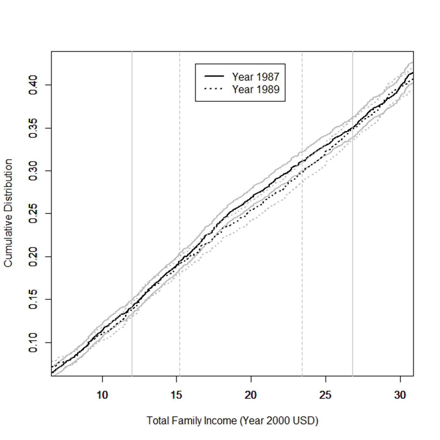
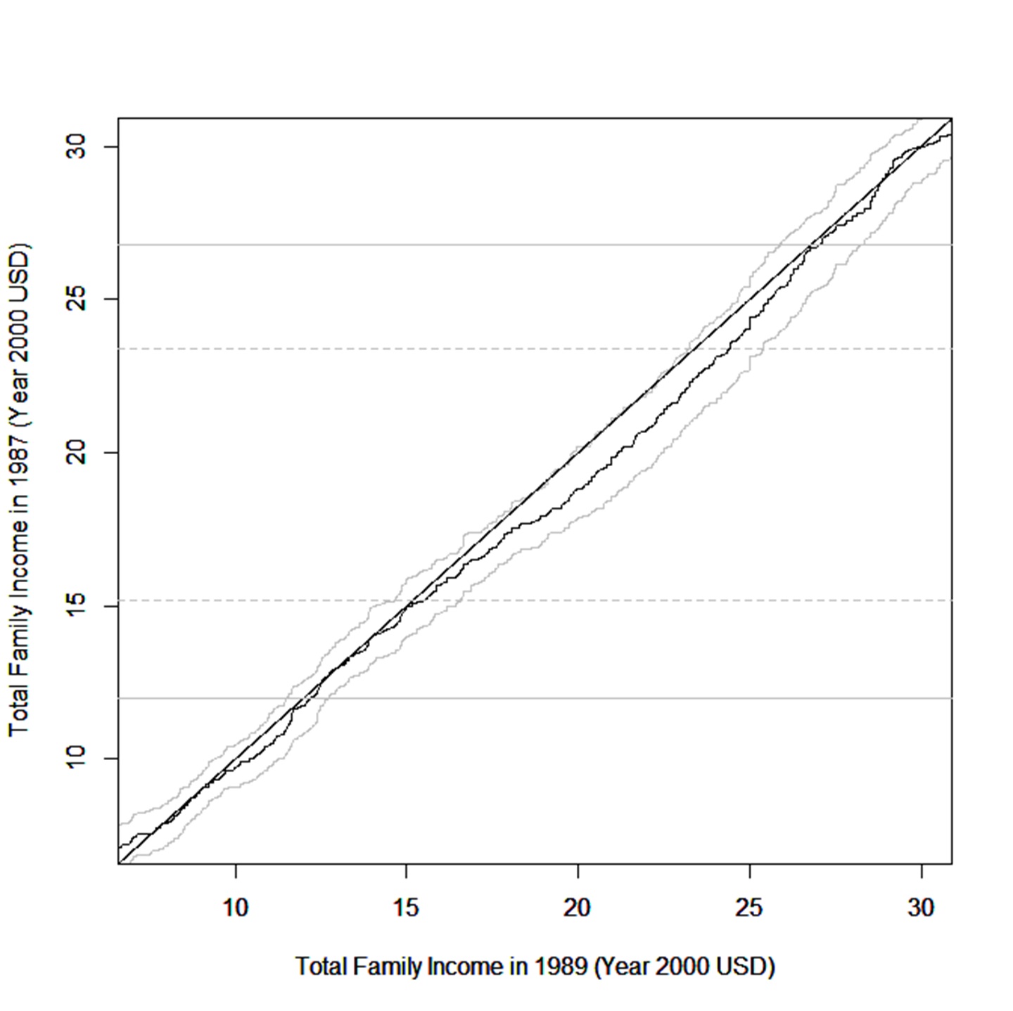
Notes: CEX data restricted to families with two or more children. Family income is given in thousands of 2000 US dollars. In the left panel, the black (resp. grey) curve corresponds to family income in 1987 (resp. 1989). In the right panel, we display the Q-Q plot, i.e. $q_{1}$ against the identity function. The solid lines indicate the theoretical limits inside which we should observe a divergence of the cdfs, given the policy design. The dotted lines are the limits of the interval on which the efffect of the policy is supposed to be maximal (see the right panel of Figure 4).

Figure 10: Cdf’s and Q-Q plot of total family income in 1987 and 1989 with bootstrap 5–95 percentiles.

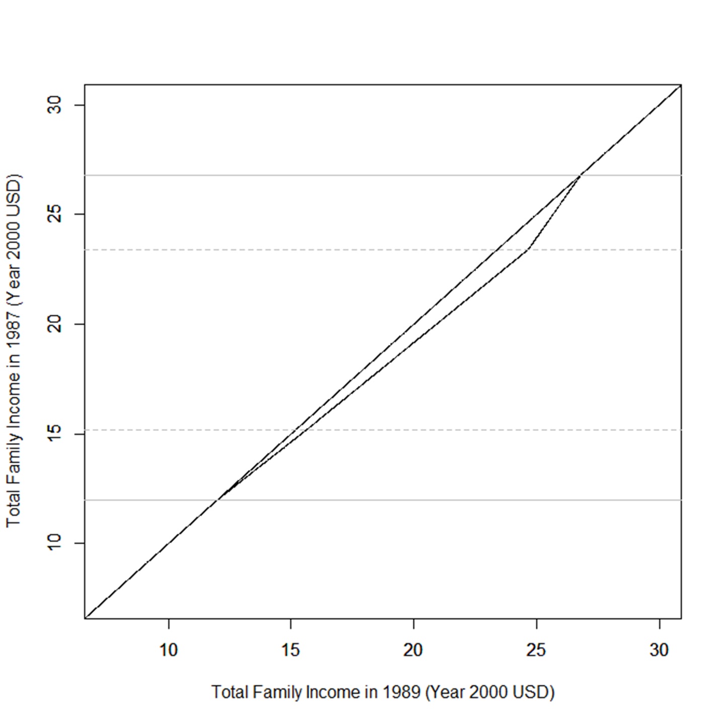
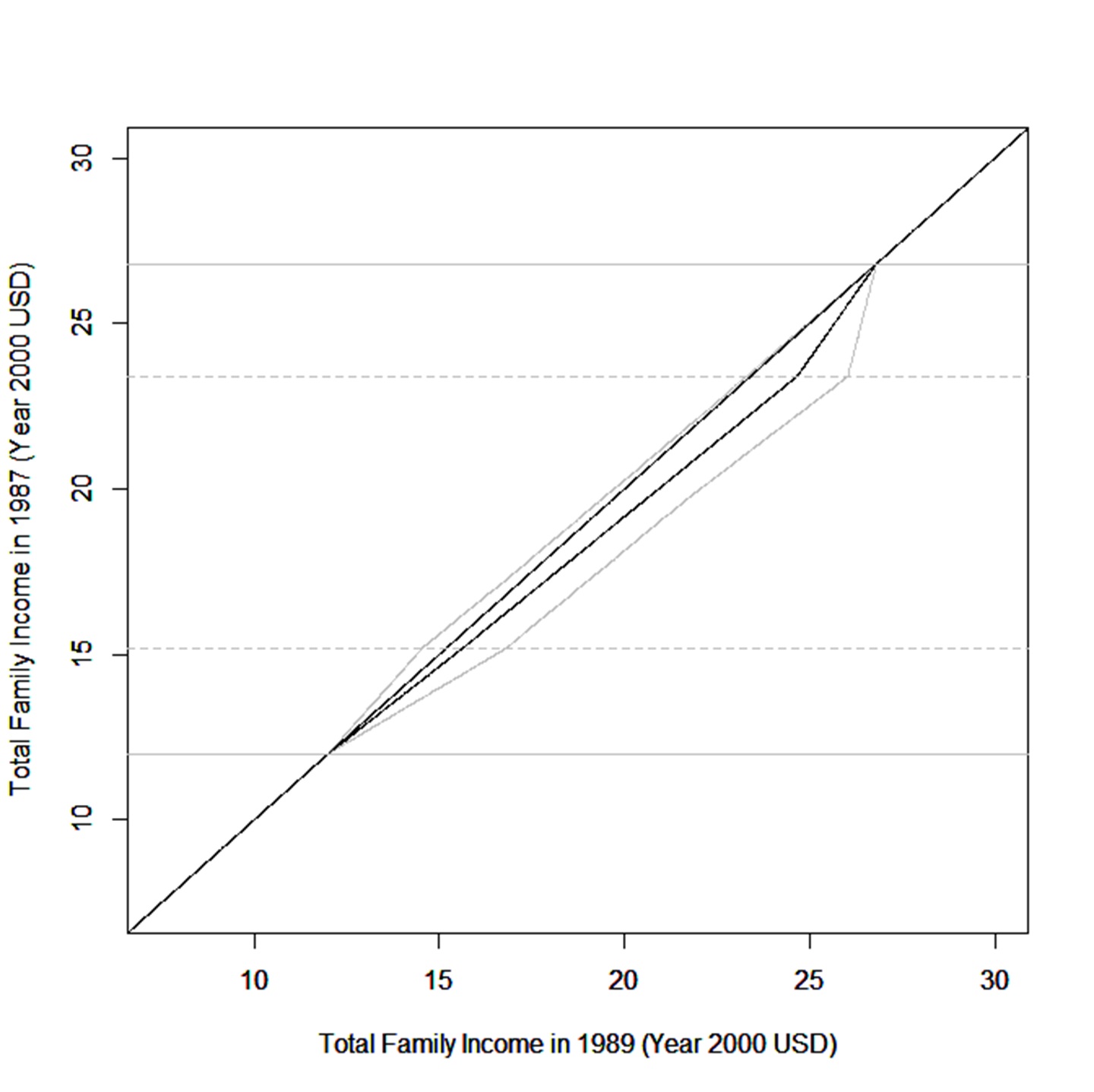
Figure 11: Piecewise linear estimator of $q_{1}$. The right panel shows bootstrap 5–95 percentiles.

Figure 12: Piecewise linear estimator of $q_{1}$ with an additional knot. The right panel shows bootstrap 5–95 percentiles.

References

- (1)
- Athey and Imbens (2006) Athey, S. and Imbens, G. W. (2006), ‘Identification and inference in nonlinear difference-in-differences models’, Econometrica 74, 431–497.
- Bierens (1987) Bierens, H. J. (1987), Kernel estimators of regression functions, in ‘Advances in econometrics: Fifth world congress’, Vol. 1, pp. 99–144.
- Blundell et al. (1993) Blundell, R., Pashardes, P. and Weber, G. (1993), ‘What do we learn about consumer demand patterns from micro data?’, The American Economic Review pp. 570–597.
- Browning and Collado (2001) Browning, M. and Collado, M. D. (2001), ‘The response of expenditures to anticipated income changes: panel data estimates’, American Economic Review 91(3), 681–692.
- Card (2001) Card, D. (2001), ‘Estimating the return to schooling: Progress on some persistent econometric problems’, Econometrica 69(5), 1127–1160.
- Chernozhukov et al. (2013) Chernozhukov, V., Fernandez-Val, I., Hahn, J. and Newey, W. (2013), ‘Average and quantile effects in non separable panel data models’, Econometrica 81, 535–580.
- Chernozhukov et al. (2015) Chernozhukov, V., Fernandez-Val, I., Hoderlein, S., Holzmann, H. and Newey, W. (2015), ‘Nonparametric identification in panels using quantiles’, Journal of Econometrics 188(2), 378–392.
- Dahl and Lochner (2012) Dahl, G. B. and Lochner, L. (2012), ‘The impact of family income on child achievement: Evidence from the earned income tax credit’, The American Economic Review 102(5), 1927–1956.
- de Chaisemartin and D’Haultfœuille (2018) de Chaisemartin, C. and D’Haultfœuille, X. (2018), ‘Fuzzy differences-in-differences’, Review of Economic Studies 85, 999–1028.
- Deaton (1992) Deaton, A. (1992), Understanding consumption, Oxford University Press.
- Einmahl and Mason (1997) Einmahl, U. and Mason, D. M. (1997), ‘Gaussian approximation of local empirical processes indexed by functions’, Probability Theory and Related Fields 107, 283–311.
- Einmahl and Mason (2000) Einmahl, U. and Mason, D. M. (2000), ‘An empirical process approach to the uniform consistency of kernel-type function estimators’, Journal of Theoretical Probability 13(1), 1–37.
- Falk (2014) Falk, G. (2014), The earned income tax credit (eitc): An overview. Washington, DC: Congressional Research Service.
- Florens et al. (2008) Florens, J., Heckman, J. J., Meghir, C. and Vytlacil, E. (2008), ‘Identification of treatment effects using control functions in models with continuous, endogenous treatment and heterogeneous effects’, Econometrica 76, 1191–1206.
- Graham and Powell (2012) Graham, B. S. and Powell, J. L. (2012), ‘Identification and estimation of average partial effects in ‘irregular’ correlated random coefficient panel data models’, Econometrica 80, 2105–2152.
- Hall (1978) Hall, R. E. (1978), ‘Stochastic implications of the life cycle-permanent income hypothesis: theory and evidence’, Journal of political economy 86(6), 971–987.
- Heckman and Vytlacil (1998) Heckman, J. and Vytlacil, E. J. (1998), ‘Instrumental variables methods for the correlated random coefficient model: Estimating the average return to schooling when the return is correlated with schooling’, Journal of Human Resources 33, 974–987.
- Hoderlein (2011) Hoderlein, S. (2011), ‘How many consumers are rational?’, Journal of Econometrics 164(2), 294–309.
- Hoderlein and White (2012) Hoderlein, S. and White, H. (2012), ‘Nonparametric identification in nonseparable panel data models with generalized fixed effects’, Journal of Econometrics 168, 300–314.
- Honore (1992) Honore, B. (1992), ‘Trimmed lad and least squares estimation of truncated and censored regression models with fixed effects’, Econometrica 60, 533–565.
- Hsieh (2003) Hsieh, C.-T. (2003), ‘Do consumers react to anticipated income changes? evidence from the alaska permanent fund’, American Economic Review 93(1), 397–405.
- Imbens and Newey (2009) Imbens, G. W. and Newey, W. K. (2009), ‘Identification and estimation of triangular simultaneous equations models without additivity’, Econometrica 77, 1481–1512.
- Jappelli and Pistaferri (2010) Jappelli, T. and Pistaferri, L. (2010), ‘The consumption response to income changes’, Annu. Rev. Econ. 2(1), 479–506.
- Johnson et al. (2006) Johnson, D. S., Parker, J. A. and Souleles, N. S. (2006), ‘Household expenditure and the income tax rebates of 2001’, American Economic Review 96(5), 1589–1610.
- Kaplan and Violante (2014) Kaplan, G. and Violante, G. L. (2014), ‘A model of the consumption response to fiscal stimulus payments’, Econometrica 82(4), 1199–1239.
- Kasy (2011) Kasy, M. (2011), ‘Identification in triangular systems using control functions’, Econometric Theory 27, 663–671.
- Manski (1987) Manski, C. F. (1987), ‘Semiparametric analysis of random effects linear models from binary panel data’, Econometrica 55, 357–362.
- Parker et al. (2013) Parker, J. A., Souleles, N. S., Johnson, D. S. and McClelland, R. (2013), ‘Consumer spending and the economic stimulus payments of 2008’, American Economic Review 103(6), 2530–53.
- Silverman (1978) Silverman, B. W. (1978), ‘Weak and strong uniform consistency of the kernel estimate of a density and its derivatives’, The Annals of Statistics 6, 177–184.
- Stute (1986) Stute, W. (1986), ‘On almost sure convergence of conditional empirical distribution functions’, The Annals of Probability pp. 891–901.
- van der Vaart (1998) van der Vaart, A. W. (1998), Asymptotic Statistics, Cambridge Series in Statistical and Probabilistic Mathematics.
- van der Vaart and Wellner (1996) van der Vaart, A. W. and Wellner, J. A. (1996), Weak convergence and Empirical Processes, Springer.