Discontinuous Galerkin and $C^{0}$-IP finite element approximation of periodic Hamilton–Jacobi–Bellman–Isaacs problems with application to numerical homogenization

Abstract.

In the first part of the paper, we study the discontinuous Galerkin (DG) and $C^{0}$ interior penalty ($C^{0}$-IP) finite element approximation of the periodic strong solution to the fully nonlinear second-order Hamilton–Jacobi–Bellman–Isaacs (HJBI) equation with coefficients satisfying the Cordes condition. We prove well-posedness and perform abstract a posteriori and a priori analyses which apply to a wide family of numerical schemes. These periodic problems arise as the corrector problems in the homogenization of HJBI equations. The second part of the paper focuses on the numerical approximation to the effective Hamiltonian of ergodic HJBI operators via DG/$C^{0}$-IP finite element approximations to approximate corrector problems. Finally, we provide numerical experiments demonstrating the performance of the numerical schemes.

1. Introduction

In the first part of this paper we study the periodic boundary value problem for the fully nonlinear second-order Hamilton–Jacobi–Bellman–Isaacs (HJBI) equation

$$\left\{\begin{aligned} \inf_{\alpha\in\mathcal{A}}\sup_{\beta\in\mathcal{B}}\left\{-A^{\alpha\beta}:\nabla^{2}u-b^{\alpha\beta}\cdot\nabla u+c^{\alpha\beta}u-f^{\alpha\beta}\right\}=0\quad\text{in }Y,\\ u\text{ is $Y$-periodic},\end{aligned}\right.$$ (1.1)

where $\mathcal{A}$ and $\mathcal{B}$ are compact metric spaces, and $Y:=(0,1)^{n}\subset\mathbb{R}^{n}$ denotes the unit cell in dimension $n\geq 2$. Here, we use the notation

$$\varphi^{\alpha\beta}:=\varphi(\,\cdot\,,\alpha,\beta),\qquad\varphi\in\{A,b,c,f\},$$

and assume that the functions

$$A=(a_{ij}):\mathbb{R}^{n}\times\mathcal{A}\times\mathcal{B}\rightarrow\mathbb{R}^{n\times n}_{\mathrm{sym}},\quad b=(b_{i}):\mathbb{R}^{n}\times\mathcal{A}\times\mathcal{B}\rightarrow\mathbb{R}^{n},\quad c,f:\mathbb{R}^{n}\times\mathcal{A}\times\mathcal{B}\rightarrow\mathbb{R}$$

are uniformly continuous and $Y$-periodic in their first argument $y\in\mathbb{R}^{n}$. Further, we assume that $A$ is uniformly elliptic (see (2.2)), that $\inf_{\mathbb{R}^{n}\times\mathcal{A}\times\mathcal{B}}c>0$, and that the coefficients $A,b,c$ satisfy the Cordes condition

$$\lvert A\rvert^{2}+\frac{\lvert b\rvert^{2}}{2\lambda}+\frac{c^{2}}{\lambda^{2}}\leq\frac{1}{n+\delta}\left(\mathrm{tr}(A)+\frac{c}{\lambda}\right)^{2}$$

in $\mathbb{R}^{n}\times\mathcal{A}\times\mathcal{B}$ for some constants $\lambda>0$ and $\delta\in(0,1)$. These assumptions guarantee the existence and uniqueness of a periodic strong solution $u\in H^{2}_{\mathrm{per}}(Y)$ to the HJBI problem (1.1); see Section 2.2.

The goal of the first part of the paper is the construction of discontinuous Galerkin (DG) and $C^{0}$ interior penalty ($C^{0}$-IP) finite element schemes for the periodic HJBI problem (1.1) and their rigorous a posteriori and a priori error analysis; see Section 2.

The fully nonlinear HJBI equation is a very general elliptic PDE arising in many contexts, such as stochastic differential games and optimal control problems. In the case that one of the metric spaces $\mathcal{A},\mathcal{B}$ is a singleton set, the HJBI equation becomes the HJB equation arising in stochastic optimal control theory, with applications in finance, engineering, and renewable energies. Interestingly, the HJBI equation is capable of capturing other famous nonlinear PDEs, such as the fully nonlinear Monge–Ampère (MA) equation arising in illumination optics, optimal transport (see Kawecki, Lakkis, Pryer [34]), and differential geometry. The MA equation is conditionally elliptic, with classical examples exhibiting a lack of uniqueness. The HJBI formulation of the MA equation is uniquely solvable and has been used in Feng, Jensen [19], Brenner, Kawecki [8] to overcome this lack of uniqueness.

The HJBI problem is well understood in the framework of viscosity solutions (see e.g., Fleming, Soner [22], Crandall, Ishii, Lions [14] and Ishii [28]), and there have been several numerical advances based on methods that enjoy a numerical analogue of the comparison principle used in the theory of viscosity solutions. Such methods include finite difference and semi-Lagrangian schemes such as Feng, Jensen [19], and also integro-differential finite element methods; see Camilli, Jakobsen [11], Salgado, Zhang [46]. However, enforcing a discrete maximum principle can be restrictive in practice and can lead to the requirement for large, or even unbounded stencils.

There is not a lot of work on finite element methods for periodic HJB/HJBI problems in the numerical analysis literature, and we refer to Gallistl, Sprekeler, Süli [24] for a mixed finite element scheme for periodic HJB problems. In recent years, there have been several advances in finite element methods for the Dirichlet problem based on the theory of the concept of strong solutions to HJBI equations. Such methods are typically more flexible than the finite difference method and allow one to capture complex geometries and to obtain higher order convergence rates. The existence and uniqueness of strong solutions to linear nondivergence-form PDEs (arising in the linearization of HJBI problems) and to the HJB equation was established in Smears, Süli [48, 49, 50], along with the well-posedness of optimal $hp$-finite element methods. These methods involved additional stabilizing forms that enforced a numerical analogue of the Miranda–Talenti estimate which is key to the well-posedness of the strong PDE. Other primal finite element methods that tackle the HJB problem are Neilan, Wu [42] and Brenner, Kawecki [8]. Here the authors use a discrete analogue of the Miranda–Talenti estimate, based on the theory of $H^{2}(\Omega)\cap H^{1}_{0}(\Omega)$ enrichment operators (see Neilan, Wu [42], Brenner, Kawecki [8], Kawecki, Smears [36, 37]), to prove strong monotonicity of the scheme without the need for an additional stabilizing bilinear form.

Following on from these approaches, these ideas have been extended from the HJB problem to the HJBI problem in Kawecki, Smears [36], and have been analyzed under a general framework that incorporates a priori and a posteriori error analysis for a wide family of finite element methods that encompasses the aforementioned schemes [48, 49, 42, 8]. In Kawecki, Smears [37], the convergence of a family of adaptive finite element schemes for HJBI problems was proven. More recently, a virtual element method for the approximation of linear nondivergence-form PDEs and HJBI problems has been proposed and analyzed in Kawecki, Pryer [35].

Alongside this, we refer the reader to the papers [10, 11, 24, 25, 29, 30] by various authors for finite element approaches allowing the use of $H^{1}$-conforming finite elements for HJB problems.

We refer to Kawecki [32] for finite element methods for linear nondivergence-form elliptic PDEs on curved domains, and to Gallistl [23], Kawecki [33] for those with oblique boundary conditions. For a survey on recent developments of numerical methods for fully nonlinear PDEs see Feng, Glowinski, Neilan [18] and Neilan, Salgado, Zhang [41].

Periodic HJBI problems of the form (1.1) arise naturally as corrector problems in the periodic homogenization of HJBI equations, which is the focus of the second part of this paper. More precisely, we are interested in the numerical approximation of the effective Hamiltonian corresponding to HJBI operators $F:\mathbb{R}^{n}\times\mathbb{R}^{n}\times\mathbb{R}^{n}\times\mathbb{R}^{n\times n}_{\mathrm{sym}}\rightarrow\mathbb{R}$ of the form

$$F(x,y,p,R):=\inf_{\alpha\in\mathcal{A}}\sup_{\beta\in\mathcal{B}}\left\{-A^{\alpha\beta}(x,y):R-b^{\alpha\beta}(x,y)\cdot p-f^{\alpha\beta}(x,y)\right\}$$

with sufficiently regular coefficients which are $Y$-periodic in $y\in\mathbb{R}^{n}$.

To any fixed point $(x,p,R)\in\mathbb{R}^{n}\times\mathbb{R}^{n}\times\mathbb{R}^{n\times n}_{\mathrm{sym}}$ we associate the approximate correctors $\{v^{\sigma}(\cdot\,;x,p,R)\}_{\sigma>0}\subset C(\mathbb{R}^{n})$, defined as the unique viscosity solutions to the cell $\sigma$-problem (see Alvarez, Bardi [5]) for parameters $\sigma>0$, that is,

$$\left\{\begin{aligned} \sigma v^{\sigma}(y;x,p,R)+F(x,y,p,R+\nabla_{y}^{2}v^{\sigma}(y;x,p,R))=0\quad\text{for }y\in Y,\\ y\mapsto v^{\sigma}(y;x,p,R)\text{ is $Y$-periodic}.\end{aligned}\right.$$

The operator $F$ is called ergodic (in the $y$-variable) at the point $(x,p,R)$ if there exists a constant $H(x,p,R)$ such that

$$-\sigma v^{\sigma}(\cdot\,;x,p,R)\underset{\sigma\searrow 0}{\longrightarrow}H(x,p,R)\quad\text{uniformly},$$

and we say $F$ is ergodic if $F$ is ergodic at every point $(x,p,R)$ and call the function

$$H:\mathbb{R}^{n}\times\mathbb{R}^{n}\times\mathbb{R}^{n\times n}_{\mathrm{sym}}\rightarrow\mathbb{R},\qquad(x,p,R)\mapsto H(x,p,R)$$

the effective Hamiltonian corresponding to $F$; see Alvarez, Bardi [5].

The cell $\sigma$-problem is an approximation to the true cell problem familiar to the reader coming from periodic homogenization (see Evans [15, 16]), that is, for fixed $(x,p,R)$ there exists at most one constant $\mu\in\mathbb{R}$ such that there exists a viscosity solution $v(\cdot\,;x,p,R)\in C(\mathbb{R}^{n})$, a corrector, to the problem

$$\left\{\begin{aligned} F(x,y,p,R+\nabla^{2}v(y;x,p,R))=\mu\quad\text{for }y\in Y,\\ y\mapsto v(y;x,p,R)\text{ is $Y$-periodic},\end{aligned}\right.$$

and when such a $\mu$ exists, $F$ is ergodic at $(x,p,R)$ and we have that $H(x,p,R)=\mu$. However, to a given ergodic operator there may be no corrector in general, and we refer to Alvarez, Bardi [2, 3, 4, 5], Alvarez, Bardi, Marchi [6], and Arisawa, Lions [7] for a detailed overview.

The goal of this second part of the paper is the construction of a numerical scheme for the approximation of the effective Hamiltonian to ergodic HJBI operators which is based on discontinuous Galerkin or $C^{0}$-IP finite element approximations to the approximate correctors; see Section 3.

The literature on numerical effective Hamiltonians to second-order HJB and HJBI operators is quite sparse. For the numerical homogenization of linear equations in nondivergence-form we refer the reader to Capdeboscq, Sprekeler, Süli [13] (see also Sprekeler, Tran [51]). The numerical homogenization of HJB equations via a mixed finite element approximation of the approximate correctors has been proposed and analyzed in Gallistl, Sprekeler, Süli [24]. A finite difference approach for numerical effective Hamiltonians to HJB operators can be found in Camilli, Marchi [12], and some exact formulas and numerical simulations for effective Hamiltonians to certain types of HJB operators are available in Finlay, Oberman [20, 21].

It seems that there are no finite element schemes for the numerical approximation of effective Hamiltonians to HJBI operators in the current literature. Let us note that there is significantly more work (see e.g., [1, 17, 26, 27, 40, 43, 44, 45]) on numerical effective Hamiltonians to first-order Hamilton–Jacobi and Hamilton–Jacobi–Isaacs equations.

This paper is organized as follows: Section 2 is focused on the DG and $C^{0}$-IP finite element approximation to the periodic HJBI problem (1.1). After proving existence and uniqueness of a periodic strong solution in Section 2.2, we discuss discretization and notation aspects in Section 2.3. We perform an a posteriori analysis independent of the choice of numerical scheme in Section 2.4, which is based on periodic enrichment and a mixed a posteriori bound. In Section 2.5, we perform an a priori error analysis for an abstract numerical scheme under natural assumptions, and present a family of numerical schemes in Section 2.5.2.

Section 3 is focused on the numerical approximation of the effective Hamiltonian to ergodic HJBI operators. We recall the definition of ergodicity and introduce the effective Hamiltonian in Section 3.1. Thereafter, in Sections 3.2 and 3.3, we present the approximation scheme for the effective Hamiltonian based on DG/$C^{0}$-IP finite element approximations to the cell $\sigma$-problem.

In Section 4, we present numerical experiments demonstrating the performance of the numerical scheme for a periodic HJBI problem (Section 4.1) and the approximation of the effective Hamiltonian to an ergodic HJBI operator (Section 4.2).

2. Discontinuous Galerkin and $C^{0}$-IP FEM for Periodic HJBI Problems

2.1. Setting

Throughout this work, we work in dimension $n\in\{2,3\}$ and write $Y:=(0,1)^{n}$ to denote the unit cell in $\mathbb{R}^{n}$. We are interested in Hamilton–Jacobi–Bellman–Isaacs (HJBI) equations posed in a periodic setting, i.e., problems of the form

$$\left\{\begin{aligned} F[u]:=\inf_{\alpha\in\mathcal{A}}\sup_{\beta\in\mathcal{B}}\left\{-A^{\alpha\beta}:\nabla^{2}u-b^{\alpha\beta}\cdot\nabla u+c^{\alpha\beta}u-f^{\alpha\beta}\right\}=0\quad\text{in }Y,\\ u\text{ is $Y$-periodic},\end{aligned}\right.$$ (2.1)

with $\mathcal{A}$ and $\mathcal{B}$ denoting compact metric spaces, and uniformly continuous functions

$$A=(a_{ij}):\mathbb{R}^{n}\times\mathcal{A}\times\mathcal{B}\rightarrow\mathbb{R}^{n\times n}_{\mathrm{sym}},\quad b=(b_{i}):\mathbb{R}^{n}\times\mathcal{A}\times\mathcal{B}\rightarrow\mathbb{R}^{n},\quad c,f:\mathbb{R}^{n}\times\mathcal{A}\times\mathcal{B}\rightarrow\mathbb{R}$$

satisfying the assumptions specified below. Here, we use the notation

$$\varphi^{\alpha\beta}(y):=\varphi(y,\alpha,\beta),\qquad y\in\mathbb{R}^{n},\;(\alpha,\beta)\in\mathcal{A}\times\mathcal{B}$$

for scalar, vector-valued or matrix-valued functions $\varphi\in C(\mathbb{R}^{n}\times\mathcal{A}\times\mathcal{B};\mathcal{R})$ with $\mathcal{R}\in\{\mathbb{R},\mathbb{R}^{n},\mathbb{R}^{n\times n}_{\mathrm{sym}}\}$.

We assume that $A^{\alpha\beta},b^{\alpha\beta},c^{\alpha\beta},f^{\alpha\beta}$ are $Y$-periodic in $y\in\mathbb{R}^{n}$ and that

$$\inf_{\mathbb{R}^{n}\times\mathcal{A}\times\mathcal{B}}c>0.$$

We further require $A$ to be uniformly elliptic, i.e.,

$$\exists\,\zeta_{1},\zeta_{2}>0:\quad\zeta_{1}\lvert\xi\rvert^{2}\leq A(y,\alpha,\beta)\xi\cdot\xi\leq\zeta_{2}\lvert\xi\rvert^{2}\qquad\forall y,\xi\in\mathbb{R}^{n},\,(\alpha,\beta)\in\mathcal{A}\times\mathcal{B},$$ (2.2)

and that the coefficients satisfy the Cordes condition (see [49]), i.e., that there holds

$$\lvert A\rvert^{2}+\frac{\lvert b\rvert^{2}}{2\lambda}+\frac{c^{2}}{\lambda^{2}}\leq\frac{1}{n+\delta}\left(\mathrm{tr}(A)+\frac{c}{\lambda}\right)^{2}$$ (2.3)

in $\mathbb{R}^{n}\times\mathcal{A}\times\mathcal{B}$ for some constants $\delta\in(0,1)$ and $\lambda>0$ (note $\lvert M\rvert:=\sqrt{M:M}$ for $M\in\mathbb{R}^{n\times n}$).

2.2. Well-posedness

In this section, we show that the periodic HJBI problem (2.1) is well-posed in the sense that there exists a unique periodic strong solution, i.e., a unique function $u\in H^{2}_{\mathrm{per}}(Y)$ satisfying $F[u]=0$ almost everywhere in $Y$. Recall that the space $H^{2}_{\mathrm{per}}(Y)\subset H^{2}(Y)$ is defined as the closure of $C^{\infty}_{\mathrm{per}}(Y):=\{\left.v\right\rvert_{Y}:v\in C^{\infty}(\mathbb{R}^{n})\text{ is $Y$-periodic}\}$ with respect to the $H^{2}$-norm.

2.2.1. The renormalized problem

Let us introduce the function $\gamma=\gamma(y,\alpha,\beta)\in C(\mathbb{R}^{n}\times\mathcal{A}\times\mathcal{B})$ defined by

$$\gamma:=\left(\lvert A\rvert^{2}+\frac{\lvert b\rvert^{2}}{2\lambda}+\frac{c^{2}}{\lambda^{2}}\right)^{-1}\left(\mathrm{tr}(A)+\frac{c}{\lambda}\right)$$ (2.4)

and note that, by the assumptions on the coefficients $A,b,c$ from Section 2.1, we have

$$\inf_{\mathbb{R}^{n}\times\mathcal{A}\times\mathcal{B}}\gamma>0.$$ (2.5)

We then consider the renormalized HJBI problem

$$\left\{\begin{aligned} F_{\gamma}[u]:=\inf_{\alpha\in\mathcal{A}}\sup_{\beta\in\mathcal{B}}\left\{\gamma^{\alpha\beta}\left(-A^{\alpha\beta}:\nabla^{2}u-b^{\alpha\beta}\cdot\nabla u+c^{\alpha\beta}u-f^{\alpha\beta}\right)\right\}=0\quad\text{in }Y,\\ u\text{ is $Y$-periodic}.\end{aligned}\right.$$ (2.6)

It is easily checked that the renormalized problem (2.6) is equivalent to the original problem (2.1) in the sense that they have the same set of periodic strong solutions. More precisely, we can characterize strong solutions to (2.1) as follows:

Remark 2.1.

For $u\in H^{2}_{\mathrm{per}}(Y)$, the following assertions are equivalent:

• $F[u]=0$ a.e. in $Y$, i.e., $u$ is a periodic strong solution to the HJBI problem (2.1).

• $F_{\gamma}[u]=0$ a.e. in $Y$, i.e., $u$ is a periodic strong solution to the renormalized problem (2.6).

• There holds

  $$\int_{Y}F_{\gamma}[u]L_{\lambda}v=0\qquad\forall v\in H^{2}_{\mathrm{per}}(Y),$$

  where $L_{\lambda}v:=\lambda v-\Delta v$ for functions $v\in H^{2}_{\mathrm{per}}(Y)$.

Indeed, the equivalence (i)$\Leftrightarrow$(ii) follows from (2.5) and the compactness of the metric spaces $\mathcal{A}$ and $\mathcal{B}$ (see also [36, Lemma 2.2]), and (ii)$\Leftrightarrow$(iii) is a consequence of the surjectivity of the linear differential operator

$$L_{\lambda}:H^{2}_{\mathrm{per}}(Y)\rightarrow L^{2}(Y),\qquad L_{\lambda}v:=\lambda v-\Delta v.$$

2.2.2. Consequences of the Cordes condition

We point out a crucial estimate for the nonlinear operator $F_{\gamma}$. This is a direct consequence of the Cordes condition (2.3) and can be found in [36]. A short proof is provided for demonstrating how the Cordes condition comes into play.

Lemma 2.1.

Let $\omega\subset Y$ be an open set. For any $u_{1},u_{2}\in H^{2}(\omega)$, writing $\delta_{u}:=u_{1}-u_{2}$, we have that

$$\left\lvert F_{\gamma}[u_{1}]-F_{\gamma}[u_{2}]-L_{\lambda}\delta_{u}\right\rvert\leq\sqrt{1-\delta}\sqrt{\lvert\nabla^{2}\delta_{u}\rvert^{2}+2\lambda\lvert\nabla\delta_{u}\rvert^{2}+\lambda^{2}\delta_{u}^{2}}$$ (2.7)

almost everywhere in $\omega$.

Proof.

Let $u_{1},u_{2}\in H^{2}(\omega)$ and set $\delta_{u}:=u_{1}-u_{2}$. Note that for any bounded sets $\{x^{\alpha\beta}\}_{(\alpha,\beta)\in\mathcal{A}\times\mathcal{B}}\subset\mathbb{R}$ and $\{y^{\alpha\beta}\}_{(\alpha,\beta)\in\mathcal{A}\times\mathcal{B}}\subset\mathbb{R}$ we have that

$$\left\lvert\inf_{\alpha\in\mathcal{A}}\sup_{\beta\in\mathcal{B}}x^{\alpha\beta}-\inf_{\alpha\in\mathcal{A}}\sup_{\beta\in\mathcal{B}}y^{\alpha\beta}\right\rvert\leq\sup_{(\alpha,\beta)\in\mathcal{A}\times\mathcal{B}}\lvert x^{\alpha\beta}-y^{\alpha\beta}\rvert.$$

This yields

$$\lvert F_{\gamma}[u_{1}]- F_{\gamma}[u_{2}]-L_{\lambda}\delta_{u}\rvert^{2}\leq\sup_{(\alpha,\beta)\in\mathcal{A}\times\mathcal{B}}\left\lvert\gamma^{\alpha\beta}\left(-A^{\alpha\beta}:\nabla^{2}\delta_{u}-b^{\alpha\beta}\cdot\nabla\delta_{u}+c^{\alpha\beta}\delta_{u}\right)+\Delta\delta_{u}-\lambda\delta_{u}\right\rvert^{2}$$

$$\leq\sup_{(\alpha,\beta)\in\mathcal{A}\times\mathcal{B}}\left\{\left\lvert-\gamma^{\alpha\beta}A^{\alpha\beta}+I\right\rvert^{2}+\frac{\lvert\gamma^{\alpha\beta}b^{\alpha\beta}\rvert^{2}}{2\lambda}+\frac{\lvert\gamma^{\alpha\beta}c^{\alpha\beta}-\lambda\rvert^{2}}{\lambda^{2}}\right\}\left(\lvert\nabla^{2}\delta_{u}\rvert^{2}+2\lambda\left\lvert\nabla\delta_{u}\right\rvert^{2}+\lambda^{2}\delta_{u}^{2}\right)$$

$$=\sup_{(\alpha,\beta)\in\mathcal{A}\times\mathcal{B}}\left\{n+1-\frac{\left(\mathrm{tr}(A^{\alpha\beta})+\frac{c^{\alpha\beta}}{\lambda}\right)^{2}}{\lvert A^{\alpha\beta}\rvert^{2}+\frac{\lvert b^{\alpha\beta}\rvert^{2}}{2\lambda}+\frac{\lvert c^{\alpha\beta}\rvert^{2}}{\lambda^{2}}}\right\}\left(\lvert\nabla^{2}\delta_{u}\rvert^{2}+2\lambda\left\lvert\nabla\delta_{u}\right\rvert^{2}+\lambda^{2}\delta_{u}^{2}\right)$$

$$\leq(1-\delta)\left(\lvert\nabla^{2}\delta_{u}\rvert^{2}+2\lambda\left\lvert\nabla\delta_{u}\right\rvert^{2}+\lambda^{2}\delta_{u}^{2}\right)$$

almost everywhere in $\omega$, where we have used the Cauchy–Schwarz inequality, simple calculation and the Cordes condition (2.3). ∎

Observe that by the triangle and Cauchy-Schwarz inequalities, we can eliminate the term $L_{\lambda}\delta_{u}$ from the left-hand side of (2.7). We thus find that, in the situation of Lemma 2.1, we have the Lipschitz-type estimate

$$\left\lvert F_{\gamma}[u_{1}]-F_{\gamma}[u_{2}]\right\rvert\leq\left(\sqrt{1-\delta}+\sqrt{n+1}\right)\sqrt{\lvert\nabla^{2}\delta_{u}\rvert^{2}+2\lambda\lvert\nabla\delta_{u}\rvert^{2}+\lambda^{2}\delta_{u}^{2}}$$ (2.8)

almost everywhere in $\omega$.

2.2.3. Existence and uniqueness of solutions

We are now in a position to prove the existence and uniqueness of periodic strong solutions to the HJBI problem (2.1). In view of Remark 2.1, let us define

$$B:H^{2}_{\mathrm{per}}(Y)\times H^{2}_{\mathrm{per}}(Y)\rightarrow\mathbb{R},\qquad B(u,v):=\int_{Y}F_{\gamma}[u]L_{\lambda}v.$$

We can now proceed as in [36] in showing that the Browder–Minty theorem applies and we obtain the following theorem:

Theorem 2.1 (Well-posedness).

In the situation of Section 2.1, there exists a unique periodic strong solution $u\in H^{2}_{\mathrm{per}}(Y)$ to the HJBI problem (2.1).

Proof.

Note that it is enough to show that $B$ satisfies the Lipschitz property

$$\lvert B(u_{1},v)-B(u_{2},v)\rvert\lesssim\|u_{1}-u_{2}\|_{H^{2}(Y)}\|v\|_{H^{2}(Y)}\qquad\forall u_{1},u_{2},v\in H^{2}_{\mathrm{per}}(Y),$$ (2.9)

and strong monotonicity, i.e.,

$$\|u_{1}-u_{2}\|_{H^{2}(Y)}^{2}\lesssim B(u_{1},u_{1}-u_{2})-B(u_{2},u_{1}-u_{2})\qquad\forall u_{1},u_{2}\in H^{2}_{\mathrm{per}}(Y).$$ (2.10)

The Browder–Minty theorem then yields that there exists a unique $u\in H^{2}_{\mathrm{per}}(Y)$ such that

$$B(u,v)=0\qquad\forall v\in H^{2}_{\mathrm{per}}(Y),$$

which proves the theorem in view of Remark 2.1.

Before we show (2.9) and (2.10), let us note that integration by parts and a density argument yields $\|\Delta v\|_{L^{2}(Y)}=\|\nabla^{2}v\|_{L^{2}(Y)}$ for any $v\in H^{2}_{\mathrm{per}}(Y)$, and hence, using integration by parts again, we have

$$\|L_{\lambda}v\|_{L^{2}(Y)}^{2}=\|\nabla^{2}v\|_{L^{2}(Y)}^{2}+2\lambda\|\nabla v\|_{L^{2}(Y)}^{2}+\lambda^{2}\|v\|_{L^{2}(Y)}^{2}\geq C_{\lambda}\|v\|_{H^{2}(Y)}^{2}\qquad\forall v\in H^{2}_{\mathrm{per}}(Y).$$ (2.11)

The Lipschitz property (2.9) now immediately follows from (2.8) and it remains to show strong monotonicity. To this end, let $u_{1},u_{2}\in H^{2}_{\mathrm{per}}(Y)$ and write $\delta_{u}:=u_{1}-u_{2}$. Using Lemma 2.1, we find

$$B(u_{1},\delta_{u})-B(u_{2},\delta_{u})=\|L_{\lambda}\delta_{u}\|_{L^{2}(Y)}^{2}+\int_{Y}\left(F_{\gamma}[u_{1}]-F_{\gamma}[u_{2}]-L_{\lambda}\delta_{u}\right)L_{\lambda}\delta_{u}\geq(1-\sqrt{1-\delta})\|L_{\lambda}\delta_{u}\|_{L^{2}(Y)}^{2}$$

and hence, by (2.11), there holds (2.10) and the claim is proved. ∎

Remark 2.2.

For the unique periodic strong solution $u\in H^{2}_{\mathrm{per}}(Y)$ to the HJBI problem (2.1), we have the bound

$$\|L_{\lambda}u\|_{L^{2}(Y)}=\sqrt{\|\nabla^{2}u\|_{L^{2}(Y)}^{2}+2\lambda\|\nabla u\|_{L^{2}(Y)}^{2}+\lambda^{2}\|u\|_{L^{2}(Y)}^{2}}\leq\frac{\|F_{\gamma}[0]\|_{L^{2}(Y)}}{1-\sqrt{1-\delta}}.$$

Proof.

Note that we have already obtained the first equality (see (2.11)). We use Lemma 2.1 and the solution property $F_{\gamma}[u]=0$ to find

$$(1-\sqrt{1-\delta})\|L_{\lambda}u\|_{L^{2}(Y)}^{2}\leq\int_{Y}(F_{\gamma}[u]-F_{\gamma}[0])L_{\lambda}u=-\int_{Y}F_{\gamma}[0]L_{\lambda}u.$$

We conclude the proof by using Hölder’s inequality to obtain

$$\|L_{\lambda}u\|_{L^{2}(Y)}^{2}\leq\frac{1}{1-\sqrt{1-\delta}}\left\lvert\int_{Y}F_{\gamma}[0]L_{\lambda}u\right\rvert\leq\frac{\|F_{\gamma}[0]\|_{L^{2}(Y)}}{1-\sqrt{1-\delta}}\|L_{\lambda}u\|_{L^{2}(Y)},$$

which yields the desired bound. ∎

2.3. Discretization

This section is devoted to discretization aspects. We introduce DG and $C^{0}$-IP finite element spaces $V^{0}_{\mathcal{T}}$ and $V^{1}_{\mathcal{T}}$ for an appropriate partition $\mathcal{T}$ of the computational domain, and define jump and average operators.

2.3.1. The partition $\mathcal{T}$

We consider a finite conforming partition $\mathcal{T}$ of the closed unit cell $\bar{Y}$ consisting of closed simplices that can be periodically extended in a $Y$-periodic fashion to $\mathbb{R}^{n}$, i.e., we require the discretization to be consistent with the identification of opposite faces by periodicity. We introduce the following mathematical objects associated with the partition $\mathcal{T}$:

• Set of faces $\mathcal{F}$ and associated unit normal $n_{F}$:
  We let $\mathcal{F}:=\mathcal{F}^{\mathrm{I}}\cup\mathcal{F}^{\mathrm{BP}}$ denote the set of $(n-1)$-dimensional faces, where $\mathcal{F}^{\mathrm{I}}$ is the set of all interior faces of $\mathcal{T}$, and $\mathcal{F}^{\mathrm{BP}}$ the set of all boundary face-pairs of $\mathcal{T}$, i.e., the boundary faces upon a periodic identification of opposite faces. For each face $F\in\mathcal{F}$, we associate a fixed choice of unit normal $n_{F}$, where we often only write $n$ for simplicity; see Figure 1.

• Shape-regularity parameter $\theta_{\mathcal{T}}$ and mesh-size function $h_{\mathcal{T}}$:
  We let $\theta_{T}:=\max\{\rho_{K}^{-1}\mathrm{diam}(K):K\in\mathcal{T}\}$ with $\rho_{K}$ being the diameter of the largest ball that can be inscribed in the element $K\in\mathcal{T}$. We further introduce $h_{\mathcal{T}}:\bar{Y}\rightarrow\mathbb{R}$ defined via $\left.h_{\mathcal{T}}\right\rvert_{\mathrm{int}(K)}:=h_{K}:=\left(\mathcal{L}^{n}(K)\right)^{\frac{1}{n}}$ for all $K\in\mathcal{T}$ and $\left.h_{\mathcal{T}}\right\rvert_{F}:=h_{F}:=\left(\mathcal{H}^{n-1}(F)\right)^{\frac{1}{n-1}}$ for all $F\in\mathcal{F}$.

Let us note that the concept of boundary face-pairs was introduced in [52] in the context of discontinuous Galerkin methods for linear elliptic periodic boundary value problems.

2.3.2. Finite element spaces $V_{\mathcal{T}}^{s}$

For fixed $\bar{p}\geq 2$, we define the discontinuous Galerkin finite element space $V_{\mathcal{T}}^{0}$ and the $C^{0}$-IP finite element space $V_{\mathcal{T}}^{1}$ by

$$V_{\mathcal{T}}^{0}:=\left\{v_{\mathcal{T}}\in L^{2}(Y):\left.v_{\mathcal{T}}\right\rvert_{K}\in\mathbb{P}_{\bar{p}}\;\forall K\in\mathcal{T}\right\}\quad\text{and}\quad V_{\mathcal{T}}^{1}:=V_{\mathcal{T}}^{0}\cap H^{1}_{\mathrm{per}}(Y),$$

where $\mathbb{P}_{\bar{p}}$ denotes the space of polynomials of degree at most $\bar{p}$.

Let us make some comments about the derivatives of functions in the finite element spaces. For a function $v\in V^{0}_{\mathcal{T}}$, we define $\nabla v\in L^{1}(Y;\mathbb{R}^{n})$ to be the piecewise gradient and $\nabla^{2}v\in L^{1}(Y;\mathbb{R}^{n\times n})$ to be the piecewise Hessian over the elements of the partition. We then define $\Delta v:=\mathrm{tr}(\nabla^{2}v)\in L^{1}(Y)$.

We equip the finite element spaces $V_{\mathcal{T}}^{s}$, $s\in\{0,1\}$, with the norm

$$\|v_{\mathcal{T}}\|_{\mathcal{T},\lambda}^{2}:=\int_{Y}\left(\lvert\nabla^{2}v_{\mathcal{T}}\rvert^{2}+2\lambda\lvert\nabla v_{\mathcal{T}}\rvert^{2}+\lambda^{2}v_{\mathcal{T}}^{2}\right)+\lvert v_{\mathcal{T}}\rvert_{J,\mathcal{T}}^{2},\quad\lvert v_{\mathcal{T}}\rvert_{J,\mathcal{T}}^{2}:=\int_{\mathcal{F}}\left(h_{\mathcal{T}}^{-1}\lvert\llbracket\nabla v_{\mathcal{T}}\rrbracket\rvert^{2}+h_{\mathcal{T}}^{-3}\lvert\llbracket v_{\mathcal{T}}\rrbracket\rvert^{2}\right)$$

for functions $v_{\mathcal{T}}\in V^{s}_{\mathcal{T}}$. In order to simplify the presentation, throughout this work we write $\int_{\mathcal{E}}:=\sum_{K\in\mathcal{E}}\int_{K}$ for collections $\mathcal{E}\subset\mathcal{T}$ of elements and $\int_{\mathcal{G}}:=\sum_{F\in\mathcal{G}}\int_{F}$ for collections $\mathcal{G}\subset\mathcal{F}$ of faces. The jump operator $\llbracket\cdot\rrbracket$ is defined in the following paragraph.

2.3.3. Jump and average operators

For elements $K\in\mathcal{T}$, we write $\tau_{\partial K}:\mathrm{BV}(K)\rightarrow L^{1}(\partial K)$ to denote the trace operator. Further, for $v\in\mathrm{BV}(Y)$ we define $\tau_{\partial K}v:=\tau_{\partial K}(\left.v\right\rvert_{K})$ for elements $K\in\mathcal{T}$. We then introduce the jump $\llbracket v\rrbracket_{F}$ and the average $\{v\}_{F}$ of a function $v\in\mathrm{BV}(Y)$ over a face $F=\partial K\cap\partial K^{\prime}\in\mathcal{F}$ shared by the elements $K,K^{\prime}\in\mathcal{T}$ by

$$\llbracket v\rrbracket_{F} :=\left.\tau_{\partial K}v\right\rvert_{F}-\left.\tau_{\partial K^{\prime}}v\right\rvert_{F}\in L^{1}(F),$$

$$\{v\}_{F} :=\frac{\left.\tau_{\partial K}v\right\rvert_{F}+\left.\tau_{\partial K^{\prime}}v\right\rvert_{F}}{2}\in L^{1}(F),$$

where $K,K^{\prime}$ are labeled such that the unit normal $n_{F}$ is the outward normal to $K$ on the face $F$; see Figure 1. To simplify the presentation, we will often simply write $\llbracket\cdot\rrbracket$ and $\{\cdot\}$, and drop the subscript.

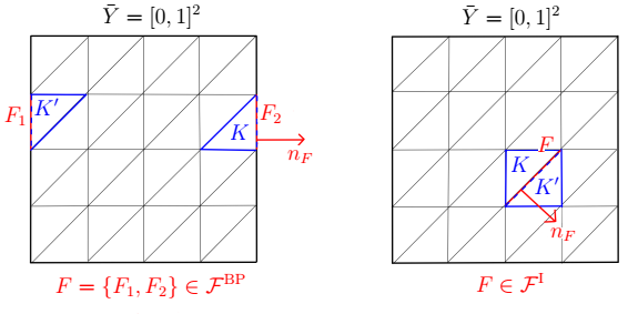
Figure 1. Illustration of a boundary face-pair $F\in\mathcal{F}^{\mathrm{BP}}$ (left) and an interior face $F\in\mathcal{F}^{\mathrm{I}}$ (right) in dimension $n=2$.

2.4. A posteriori analysis

Let $u\in H^{2}_{\mathrm{per}}(Y)$ denote the unique solution to the HJBI problem (2.1) and let $v_{\mathcal{T}}\in V^{0}_{\mathcal{T}}$ be arbitrary. The goal of this section is to estimate the $\|\cdot\|_{\mathcal{T},\lambda}$-distance between $u$ and $v_{\mathcal{T}}$, i.e.,

$$\|u-v_{\mathcal{T}}\|_{\mathcal{T},\lambda}^{2}=\int_{Y}\left(\lvert\nabla^{2}(u-v_{\mathcal{T}})\rvert^{2}+2\lambda\lvert\nabla(u-v_{\mathcal{T}})\rvert^{2}+\lambda^{2}(u-v_{\mathcal{T}})^{2}\right)+\lvert u-v_{\mathcal{T}}\rvert_{J,\mathcal{T}}^{2},$$

in terms of a computable quantity not depending on the solution $u$. We start by introducing periodic enrichment operators which are an important tool in establishing the a posteriori bound.

2.4.1. Periodic enrichment

We let $\mathcal{Z}$ be the set of points in $\bar{Y}$ corresponding to the Lagrange degrees of freedom for the function space $V^{1}_{\mathcal{T}}=V^{0}_{\mathcal{T}}\cap H^{1}_{\mathrm{per}}(Y)$, where boundary nodes on $\partial Y$ are identified with all their $Y$-periodic counterparts. For $z\in\mathcal{Z}$, we then define the periodic neighborhood $N(z)\subset\mathcal{T}$ to be the set of all elements $K\in\mathcal{T}$ that contain $z$ or any periodically identical point to $z$; see Figure 2.

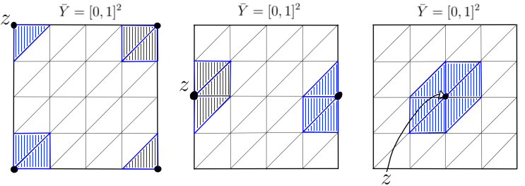
Figure 2. Illustration of the periodic neighborhood $N(z)\subset\mathcal{T}$ in dimension $n=2$. Left: $z\in\mathcal{Z}\cap\partial Y$ corner point, middle: $z\in\mathcal{Z}\cap\partial Y$ non-corner boundary point, right: $z\in\mathcal{Z}\cap Y$ interior point.

Let us introduce an operator

$$E_{1}:V^{0}_{\mathcal{T}}\rightarrow V^{0}_{\mathcal{T}}\cap H^{1}_{\mathrm{per}}(Y),$$

which we call the $H^{1}_{\mathrm{per}}$-enrichment operator, defined through averaging of the function values in periodic neighborhoods of points in $\mathcal{Z}$. That is, for $v_{\mathcal{T}}\in V^{0}_{\mathcal{T}}$, we define the function $E_{1}v_{\mathcal{T}}\in V^{1}_{\mathcal{T}}$ by prescribing

$$E_{1}v_{\mathcal{T}}(z):=\frac{1}{\lvert N(z)\rvert}\sum_{K\in N(z)}\left.v_{\mathcal{T}}\right\rvert_{K}(z)$$

at points $z\in\mathcal{Z}$. Denoting the collection of interior faces and boundary face-pairs neighboring an element $K\in\mathcal{T}$ by $\mathcal{F}_{K}:=\{F\in\mathcal{F}:F\cap K\neq\emptyset\}$, we then have the bound

$$\sum_{m=0}^{2}\int_{K}h_{\mathcal{T}}^{2m-4}\left\lvert\nabla^{m}(v_{\mathcal{T}}-E_{1}v_{\mathcal{T}})\right\rvert^{2}\lesssim\int_{\mathcal{F}_{K}}h_{\mathcal{T}}^{-3}\lvert\llbracket v_{\mathcal{T}}\rrbracket\rvert^{2}\qquad\forall K\in\mathcal{T}$$ (2.12)

for all $v_{\mathcal{T}}\in V^{0}_{\mathcal{T}}$, where the constant absorbed in $\lesssim$ only depends on $n,\theta_{\mathcal{T}}$ and $\bar{p}$. This bound follows from the arguments in [31].

Let us also discuss the periodic enrichment of vector fields. To this end, we define the space containing potential gradients of functions in the finite element spaces by

$$W_{\mathcal{T}}:=\{v_{\mathcal{T}}\in L^{2}(Y;\mathbb{R}^{n}):\left.v_{\mathcal{T}}\right\rvert_{K}\in\mathbb{P}_{\bar{p}-1}^{n}\;\forall K\in\mathcal{T}\}.$$

Indeed, observe that $\nabla v_{\mathcal{T}}\in W_{\mathcal{T}}$ for any $v_{\mathcal{T}}\in V^{s}_{\mathcal{T}}$, $s\in\{0,1\}$. Analogously to $E_{1}$, we can then construct a linear operator

$$E_{1}^{g}:W_{\mathcal{T}}\rightarrow W_{\mathcal{T}}\cap H^{1}_{\mathrm{per}}(Y;\mathbb{R}^{n})$$

satisfying

$$\int_{K}\left(\left\lvert\nabla(w_{\mathcal{T}}-E_{1}^{g}w_{\mathcal{T}})\right\rvert^{2}+h_{\mathcal{T}}^{-2}\left\lvert w_{\mathcal{T}}-E_{1}^{g}w_{\mathcal{T}}\right\rvert^{2}\right)\lesssim\int_{\mathcal{F}_{K}}h_{\mathcal{T}}^{-1}\lvert\llbracket w_{\mathcal{T}}\rrbracket\rvert^{2}\qquad\forall K\in\mathcal{T}$$ (2.13)

for all $w_{\mathcal{T}}\in W_{\mathcal{T}}$, where the constant absorbed in $\lesssim$ only depends on $n,\theta_{\mathcal{T}}$ and $\bar{p}$. With the enrichment operators at hand we can proceed with the a posteriori analysis, independent of the choice of the numerical scheme.

2.4.2. The a posteriori bound

It will be useful to introduce some notation from the mixed finite element theory developed in [24]. Let us consider the function space

$$X:=W_{\mathrm{per}}(Y;\mathbb{R}^{n})\times H^{1}_{\mathrm{per}}(Y),$$

which we equip with the ${\left|\kern-1.07639pt\left|\kern-1.07639pt\left|\cdot\right|\kern-1.07639pt\right|\kern-1.07639pt\right|}_{\lambda}$-norm given by

$${\left|\kern-1.07639pt\left|\kern-1.07639pt\left|(w^{\prime},u^{\prime})\right|\kern-1.07639pt\right|\kern-1.07639pt\right|}_{\lambda}^{2}:=\|\nabla w^{\prime}\|_{L^{2}(Y)}^{2}+2\lambda\|\nabla u^{\prime}\|_{L^{2}(Y)}^{2}+\lambda^{2}\|u^{\prime}\|_{L^{2}(Y)}^{2},\qquad(w^{\prime},u^{\prime})\in X.$$

We recall that the spaces $W_{\mathrm{per}}(Y)\subset H^{1}_{\mathrm{per}}(Y)$ and $W_{\mathrm{per}}(Y;\mathbb{R}^{n})\subset H^{1}_{\mathrm{per}}(Y;\mathbb{R}^{n})$ are defined as

$$W_{\mathrm{per}}(Y):=\left\{v\in H^{1}_{\mathrm{per}}(Y):\int_{Y}v=0\right\},\qquad W_{\mathrm{per}}(Y;\mathbb{R}^{n}):=\left(W_{\mathrm{per}}(Y)\right)^{n}.$$

We further define the mixed analogue $F_{\gamma}^{M}$ to the nonlinear operator $F_{\gamma}$ by

$$F_{\gamma}^{M}[(w^{\prime},u^{\prime})]:=\inf_{\alpha\in\mathcal{A}}\sup_{\beta\in\mathcal{B}}\left\{\gamma^{\alpha\beta}\left(-A^{\alpha\beta}:\nabla w^{\prime}-b^{\alpha\beta}\cdot\nabla u^{\prime}+c^{\alpha\beta}u^{\prime}-f^{\alpha\beta}\right)\right\}$$

for pairs $(w^{\prime},u^{\prime})\in X$, and observe that the solution $u\in H^{2}_{\mathrm{per}}(Y)$ to (2.1) satisfies

$$F_{\gamma}^{M}[(\nabla u,u)]=F_{\gamma}[u]=0\quad\text{a.e. in }Y.$$ (2.14)

We can use the arguments from [24] to prove an a posteriori bound on the ${\left|\kern-1.07639pt\left|\kern-1.07639pt\left|\cdot\right|\kern-1.07639pt\right|\kern-1.07639pt\right|}_{\lambda}$-distance between the solution pair $(\nabla u,u)$ and an arbitrary pair $(w^{\prime},u^{\prime})\in X$.

Lemma 2.2.

Let $u\in H^{2}_{\mathrm{per}}(Y)$ denote the unique solution to the HJBI problem (2.1). Then we have

$${\left|\kern-1.07639pt\left|\kern-1.07639pt\left|(\nabla u-w^{\prime},u-u^{\prime})\right|\kern-1.07639pt\right|\kern-1.07639pt\right|}_{\lambda}^{2}\lesssim\|F_{\gamma}^{M}[(w^{\prime},u^{\prime})]\|_{L^{2}(Y)}^{2}+\|\mathrm{rot}(w^{\prime})\|_{L^{2}(Y)}^{2}+\|\nabla u^{\prime}-w^{\prime}\|_{L^{2}(Y)}^{2}\quad\forall\,(w^{\prime},u^{\prime})\in X$$

with the constant absorbed in $\lesssim$ only depending on the Cordes parameters $\delta,\lambda$.

Proof.

We define the semilinear form $a^{M}:X\times X\rightarrow\mathbb{R}$ by

$$a^{M}\left((w_{1},u_{1}),(w_{2},u_{2})\right)$$

$$\quad:=\int_{Y}F_{\gamma}^{M}[(w_{1},u_{1})](\lambda u_{2}-\nabla\cdot w_{2})+\sigma_{1}\int_{Y}\mathrm{rot}(w_{1})\cdot\mathrm{rot}(w_{2})+\sigma_{2}\int_{Y}(\nabla u_{1}-w_{1})\cdot(\nabla u_{2}-w_{2})$$

with $\sigma_{1},\sigma_{2}>0$ given by

$$\sigma_{1}:=1-\frac{1}{2}\sqrt{1-\delta},\qquad\sigma_{2}:=\frac{\lambda}{2}(1-\sqrt{1-\delta})+\frac{\lambda}{4}(1-\sqrt{1-\delta})^{-1}.$$

A straightforward adaptation of the proof of [24, Lemma 2.3] yields the monotonicity estimate

$$C_{\delta}{\left|\kern-1.07639pt\left|\kern-1.07639pt\left|(w_{1}-w_{2},u_{1}-u_{2})\right|\kern-1.07639pt\right|\kern-1.07639pt\right|}_{\lambda}^{2}\leq a^{M}\left((w_{1},u_{1}),(w_{1}-w_{2},u_{1}-u_{2})\right)-a^{M}\left((w_{2},u_{2}),(w_{1}-w_{2},u_{1}-u_{2})\right)$$

for all $(w_{1},u_{1}),(w_{2},u_{2})\in X$, where $C_{\delta}>0$ is a constant only depending on $\delta$. In particular, in view of (2.14), we find that

$$C_{\delta}{\left|\kern-1.07639pt\left|\kern-1.07639pt\left|(\nabla u-w^{\prime},u-u^{\prime})\right|\kern-1.07639pt\right|\kern-1.07639pt\right|}_{\lambda}^{2}\leq-a^{M}\left((w^{\prime},u^{\prime}),(\nabla u-w^{\prime},u-u^{\prime})\right)\qquad\forall\,(w^{\prime},u^{\prime})\in X.$$ (2.15)

Let $(w^{\prime},u^{\prime})\in X$ be arbitrary and write $(\delta_{w},\delta_{u}):=(\nabla u-w^{\prime},u-u^{\prime})$. Using the Cauchy–Schwarz and Young inequalities to bound the right-hand side of (2.15), we have

$$C_{\delta} {\left|\kern-1.07639pt\left|\kern-1.07639pt\left|(\delta_{w},\delta_{u})\right|\kern-1.07639pt\right|\kern-1.07639pt\right|}_{\lambda}^{2}\leq\left\lvert a^{M}\left((w^{\prime},u^{\prime}),(\delta_{w},\delta_{u})\right)\right\rvert$$

$$\hskip 28.45274pt\leq\frac{1}{C_{\delta}}\|F_{\gamma}^{M}[(w^{\prime},u^{\prime})]\|_{L^{2}(Y)}^{2}+\frac{C_{\delta}}{4}\|\lambda\delta_{u}-\nabla\cdot\delta_{w}\|_{L^{2}(Y)}^{2}+\sigma_{1}\|\mathrm{rot}(w^{\prime})\|_{L^{2}(Y)}^{2}+\sigma_{2}\|\nabla u^{\prime}-w^{\prime}\|_{L^{2}(Y)}^{2}$$

and we can conclude that

$${\left|\kern-1.07639pt\left|\kern-1.07639pt\left|(\delta_{w},\delta_{u})\right|\kern-1.07639pt\right|\kern-1.07639pt\right|}_{\lambda}^{2}\leq\frac{1}{C_{\delta}^{2}}\|F_{\gamma}^{M}[(w^{\prime},u^{\prime})]\|_{L^{2}(Y)}^{2}+\frac{1}{2}{\left|\kern-1.07639pt\left|\kern-1.07639pt\left|(\delta_{w},\delta_{u})\right|\kern-1.07639pt\right|\kern-1.07639pt\right|}_{\lambda}^{2}+\frac{\sigma_{1}}{C_{\delta}}\|\mathrm{rot}(w^{\prime})\|_{L^{2}(Y)}^{2}+\frac{\sigma_{2}}{C_{\delta}}\|\nabla u^{\prime}-w^{\prime}\|_{L^{2}(Y)}^{2}$$

upon noting $\|\nabla\cdot\delta_{w}\|_{L^{2}(Y)}\leq\|\nabla\delta_{w}\|_{L^{2}(Y)}$ as $\delta_{w}\in H^{1}_{\mathrm{per}}(Y;\mathbb{R}^{n})$; see [24]. Finally, absorbing the term $\frac{1}{2}{\left|\kern-1.07639pt\left|\kern-1.07639pt\left|(\delta_{w},\delta_{u})\right|\kern-1.07639pt\right|\kern-1.07639pt\right|}_{\lambda}^{2}$ into the left-hand side of the above inequality, we obtain the desired estimate. ∎

We can use Lemma 2.2 and the $H^{1}_{\mathrm{per}}$-enrichment operators to prove the following a posteriori error bound:

Theorem 2.2 (a posteriori error bound).

Let $u\in H^{2}_{\mathrm{per}}(Y)$ denote the unique solution to the HJBI problem (2.1). Then there holds

$$\|u-v_{\mathcal{T}}\|_{\mathcal{T},\lambda}^{2}\lesssim\int_{Y}\left\lvert F_{\gamma}[v_{\mathcal{T}}]\right\rvert^{2}+\lvert v_{\mathcal{T}}\rvert_{J,\mathcal{T}}^{2}\qquad\forall v_{\mathcal{T}}\in V^{0}_{\mathcal{T}}$$

with the constant absorbed in $\lesssim$ only depending on $n,\theta_{\mathcal{T}},\bar{p}$ and the Cordes parameters $\delta,\lambda$.

Proof.

Let $v_{\mathcal{T}}\in V^{0}_{\mathcal{T}}$ be arbitrary and set

$$v :=E_{1}v_{\mathcal{T}}\in V^{0}_{\mathcal{T}}\cap H^{1}_{\mathrm{per}}(Y),$$

$$w :=E_{1}^{g}(\nabla v_{\mathcal{T}})-\int_{Y}E_{1}^{g}(\nabla v_{\mathcal{T}})\in W_{\mathcal{T}}\cap W_{\mathrm{per}}(Y;\mathbb{R}^{n}).$$

By the triangle inequality, we have

$$\|u-v_{\mathcal{T}}\|_{\mathcal{T},\lambda}^{2} \lesssim{\left|\kern-1.07639pt\left|\kern-1.07639pt\left|(\nabla u-w,u-v)\right|\kern-1.07639pt\right|\kern-1.07639pt\right|}_{\lambda}^{2}$$

$$\quad+\int_{Y}\left(\lvert\nabla(w-\nabla v_{\mathcal{T}})\rvert^{2}+2\lambda\lvert\nabla(v-v_{\mathcal{T}})\rvert^{2}+\lambda^{2}(v-v_{\mathcal{T}})^{2}\right)+\lvert v_{\mathcal{T}}\rvert_{J,\mathcal{T}}^{2},$$

which we can further bound, using the properties of the enrichment operators (2.12) and (2.13), to obtain that

$$\|u-v_{\mathcal{T}}\|_{\mathcal{T},\lambda}^{2}\lesssim{\left|\kern-1.07639pt\left|\kern-1.07639pt\left|(\nabla u-w,u-v)\right|\kern-1.07639pt\right|\kern-1.07639pt\right|}_{\lambda}^{2}+\lvert v_{\mathcal{T}}\rvert_{J,\mathcal{T}}^{2}.$$

We can apply Lemma 2.2 to find

$$\|u-v_{\mathcal{T}}\|_{\mathcal{T},\lambda}^{2}\lesssim\|F_{\gamma}^{M}[(w,v)]\|_{L^{2}(Y)}^{2}+\|\mathrm{rot}(w)\|_{L^{2}(Y)}^{2}+\|\nabla v-w\|_{L^{2}(Y)}^{2}+\lvert v_{\mathcal{T}}\rvert_{J,\mathcal{T}}^{2}.$$ (2.16)

Note that, using the triangle and Hölder inequalities, and the enrichment bounds (2.12) and (2.13), we have

$$\|\mathrm{rot}(w)\|_{L^{2}(Y)}^{2}=\int_{Y}\lvert\mathrm{rot}(w-\nabla v_{\mathcal{T}})\rvert^{2}\lesssim\lvert v_{\mathcal{T}}\rvert_{J,\mathcal{T}}^{2}$$

for the second term on the right-hand side of (2.16), and

$$\|\nabla v-w\|_{L^{2}(Y)}^{2} \lesssim\left\|\nabla v-E_{1}^{g}(\nabla v_{\mathcal{T}})-\int_{Y}\left(\nabla v-E_{1}^{g}(\nabla v_{\mathcal{T}})\right)\right\|_{L^{2}(Y)}^{2}$$

$$\lesssim\left\|\nabla v-E_{1}^{g}(\nabla v_{\mathcal{T}})\right\|_{L^{2}(Y)}^{2}$$

$$\lesssim\int_{Y}\lvert\nabla(v-v_{\mathcal{T}})\rvert^{2}+\int_{Y}\lvert\nabla v_{\mathcal{T}}-E_{1}^{g}(\nabla v_{\mathcal{T}})\rvert^{2}$$

$$\lesssim\lvert v_{\mathcal{T}}\rvert_{J,\mathcal{T}}^{2}$$

for the third term on the right-hand side of (2.16) (note that $\int_{Y}\nabla v=0$ for $v\in H^{1}_{\mathrm{per}}(Y)$). Finally, for the first term on the right-hand side of (2.16), we successively use the triangle inequality together with $F_{\gamma}[v_{\mathcal{T}}]=F_{\gamma}^{M}[(\nabla v_{\mathcal{T}},v_{\mathcal{T}})]$, a Lipschitz property of $F_{\gamma}^{M}$ which is shown analogously to (2.8), and the enrichment bounds (2.12) and (2.13) to obtain

$$\|F_{\gamma}^{M}[(w,v)]\|_{L^{2}(Y)}^{2} \lesssim\int_{Y}\left\lvert F_{\gamma}[v_{\mathcal{T}}]\right\rvert^{2}+\int_{Y}\left\lvert F_{\gamma}^{M}[(w,v)]-F_{\gamma}^{M}[(\nabla v_{\mathcal{T}},v_{\mathcal{T}})]\right\rvert^{2}$$

$$\lesssim\int_{Y}\left\lvert F_{\gamma}[v_{\mathcal{T}}]\right\rvert^{2}+\int_{Y}\left(\lvert\nabla(w-\nabla v_{\mathcal{T}})\rvert^{2}+2\lambda\lvert\nabla(v-v_{\mathcal{T}})\rvert^{2}+\lambda^{2}\lvert v-v_{\mathcal{T}}\rvert^{2}\right)$$

$$\lesssim\int_{Y}\left\lvert F_{\gamma}[v_{\mathcal{T}}]\right\rvert^{2}+\lvert v_{\mathcal{T}}\rvert_{J,\mathcal{T}}^{2}.$$

Altogether, in view of (2.16), we have proved the desired estimate. ∎

This concludes the a posteriori analysis and we proceed with an abstract a priori analysis for a wide class of numerical schemes in the next section.

2.5. Numerical scheme and a priori analysis

Let us consider an abstract numerical scheme written in the following form: For chosen $s\in\{0,1\}$, find a function $u_{\mathcal{T}}\in V^{s}_{\mathcal{T}}$ satisfying

$$a_{\mathcal{T}}(u_{\mathcal{T}},v_{\mathcal{T}})=0\qquad\forall v_{\mathcal{T}}\in V_{\mathcal{T}}^{s}.$$ (2.17)

2.5.1. Abstract a priori analysis

Here, we assume that the nonlinear form $a_{\mathcal{T}}:V_{\mathcal{T}}^{s}\times V_{\mathcal{T}}^{s}\rightarrow\mathbb{R}$ satisfies the assumptions listed below:

• Linearity in second argument: $a_{\mathcal{T}}(w_{\mathcal{T}},\cdot\,):V_{\mathcal{T}}^{s}\rightarrow\mathbb{R}$ is linear for any fixed $w_{\mathcal{T}}\in V_{\mathcal{T}}^{s}$.

• Strong monotonicity: There exists a constant $C_{M}>0$ such that

  $$\|w_{\mathcal{T}}-v_{\mathcal{T}}\|^{2}_{\mathcal{T},\lambda}\leq C_{M}\left(a_{\mathcal{T}}(w_{\mathcal{T}},w_{\mathcal{T}}-v_{\mathcal{T}})-a_{\mathcal{T}}(v_{\mathcal{T}},w_{\mathcal{T}}-v_{\mathcal{T}})\right)\qquad\forall w_{\mathcal{T}},v_{\mathcal{T}}\in V^{s}_{\mathcal{T}}.$$

• Lipschitz continuity: There exists a constant $C_{L}>0$ such that

  $$\left\lvert a_{\mathcal{T}}(w_{\mathcal{T}},v_{\mathcal{T}})-a_{\mathcal{T}}(w_{\mathcal{T}}^{\prime},v_{\mathcal{T}})\right\rvert\leq C_{L}\|w_{\mathcal{T}}-w^{\prime}_{\mathcal{T}}\|_{\mathcal{T},\lambda}\|v_{\mathcal{T}}\|_{\mathcal{T},\lambda}\qquad\forall w_{\mathcal{T}},w^{\prime}_{\mathcal{T}},v_{\mathcal{T}}\in V^{s}_{\mathcal{T}}.$$

• Discrete consistency: There exists a linear operator $L_{\mathcal{T}}:V^{s}_{\mathcal{T}}\rightarrow L^{2}(Y)$ such that, for some constant $C_{1}>0$, we have

  $$\|L_{\mathcal{T}}v_{\mathcal{T}}\|_{L^{2}(Y)}\leq C_{1}\|v_{\mathcal{T}}\|_{\mathcal{T},\lambda}\qquad\forall v_{\mathcal{T}}\in V^{s}_{\mathcal{T}},$$

  and, for some constant $C_{2}>0$, we have

  $$\left\lvert a(w_{\mathcal{T}},v_{\mathcal{T}})-\int_{Y}F_{\gamma}[w_{\mathcal{T}}]L_{\mathcal{T}}v_{\mathcal{T}}\right\rvert\leq C_{2}\lvert w_{\mathcal{T}}\rvert_{J,\mathcal{T}}\|v_{\mathcal{T}}\|_{\mathcal{T},\lambda}\qquad\forall w_{\mathcal{T}},v_{\mathcal{T}}\in V^{s}_{\mathcal{T}}.$$

Observe that the assumptions (A1)–(A4) guarantee well-posedness of the numerical scheme, that is, there exists a unique solution $u_{\mathcal{T}}\in V^{s}_{\mathcal{T}}$ satisfying (2.17). We can show an a priori bound in this general setting similarly to [36].

Theorem 2.3 (a priori error bound).

For chosen $s\in\{0,1\}$, let $a_{\mathcal{T}}:V^{s}_{\mathcal{T}}\times V^{s}_{\mathcal{T}}\rightarrow\mathbb{R}$ be a nonlinear form satisfying the assumptions (A1)–(A4). Further, let $u\in H^{2}_{\mathrm{per}}(Y)$ denote the unique solution to the HJBI problem (2.1). Then, there exists a unique solution $u_{\mathcal{T}}\in V^{s}_{\mathcal{T}}$ to (2.17) and we have the near-best approximation bound

$$\|u-u_{\mathcal{T}}\|_{\mathcal{T},\lambda}\leq C_{e}\inf_{v_{\mathcal{T}}\in V^{s}_{\mathcal{T}}}\|u-v_{\mathcal{T}}\|_{\mathcal{T},\lambda},$$ (2.18)

where the constant $C_{e}>0$ is given by

$$C_{e}:=1+C_{M}\left(C_{1}\left(\sqrt{1-\delta}+\sqrt{n+1}\right)+C_{2}\right).$$ (2.19)

Proof.

As we have already noted, the existence and uniqueness of a solution $u_{\mathcal{T}}\in V^{s}_{\mathcal{T}}$ to (2.17) follows from the assumptions on the nonlinear form $a_{\mathcal{T}}$, and it only remains to show the near-best approximation bound (2.18). To this end, let $v_{\mathcal{T}}\in V^{s}_{\mathcal{T}}$ be arbitrary and observe that

$$\begin{split}\|v_{\mathcal{T}}-u_{\mathcal{T}}\|_{\mathcal{T},\lambda}^{2}&\leq C_{M}\left(a_{\mathcal{T}}(v_{\mathcal{T}},v_{\mathcal{T}}-u_{\mathcal{T}})-a_{\mathcal{T}}(u_{\mathcal{T}},v_{\mathcal{T}}-u_{\mathcal{T}})\right)\\ &=C_{M}a_{\mathcal{T}}(v_{\mathcal{T}},v_{\mathcal{T}}-u_{\mathcal{T}})\end{split}$$ (2.20)

by strong monotonicity (A2) and the solution property (2.17) of $u_{\mathcal{T}}$. In order to further bound the right-hand side, we successively use the discrete consistency (A4), the solution property and regularity of $u$, and the Lipschitz property (2.8) of $F_{\gamma}$ to obtain

$$a_{\mathcal{T}}(v_{\mathcal{T}},v_{\mathcal{T}}-u_{\mathcal{T}}) \leq\left\lvert\int_{Y}F_{\gamma}[v_{\mathcal{T}}]L_{\mathcal{T}}(v_{\mathcal{T}}-u_{\mathcal{T}})\right\rvert+C_{2}\lvert v_{\mathcal{T}}\rvert_{J,\mathcal{T}}\|v_{\mathcal{T}}-u_{\mathcal{T}}\|_{\mathcal{T},\lambda}$$

$$\leq\left(C_{1}\|F_{\gamma}[v_{\mathcal{T}}]-F_{\gamma}[u]\|_{L^{2}(Y)}+C_{2}\lvert v_{\mathcal{T}}-u\rvert_{J,\mathcal{T}}\right)\|v_{\mathcal{T}}-u_{\mathcal{T}}\|_{\mathcal{T},\lambda}$$

$$\leq\left(C_{1}\left(\sqrt{1-\delta}+\sqrt{n+1}\right)+C_{2}\right)\|v_{\mathcal{T}}-u\|_{\mathcal{T},\lambda}\|v_{\mathcal{T}}-u_{\mathcal{T}}\|_{\mathcal{T},\lambda}.$$

Combination with the previous estimate (2.20) yields

$$\|v_{\mathcal{T}}-u_{\mathcal{T}}\|_{\mathcal{T},\lambda}\leq C_{M}\left(C_{1}\left(\sqrt{1-\delta}+\sqrt{n+1}\right)+C_{2}\right)\|u-v_{\mathcal{T}}\|_{\mathcal{T},\lambda},$$

which in turn implies

$$\|u-u_{\mathcal{T}}\|_{\mathcal{T},\lambda}\leq\|u-v_{\mathcal{T}}\|_{\mathcal{T},\lambda}+\|v_{\mathcal{T}}-u_{\mathcal{T}}\|_{\mathcal{T},\lambda}\leq C_{e}\|u-v_{\mathcal{T}}\|_{\mathcal{T},\lambda}$$

with $C_{e}>0$ given by (2.19). We conclude the proof by taking the infimum over $v_{\mathcal{T}}\in V^{s}_{\mathcal{T}}$. ∎

We conclude this section by noting that Theorem 2.3 implies convergence of the numerical approximation under mesh-refinement. While convergence together with optimal rates follow immediately from standard approximation arguments in the case that the exact solution satisfies additional regularity assumptions, it is not that clear when we only have a minimal regularity solution $u\in H^{2}_{\mathrm{per}}(Y)$. For the latter case, we can argue as in [36, Corollary 4.7] and obtain the following result.

Remark 2.3 (Convergence of the numerical approximation).

For a sequence of conforming simplicial meshes $\{\mathcal{T}_{k}\}_{k}$ with $\max_{K\in\mathcal{T}_{k}}h_{K}\rightarrow 0$ as $k\rightarrow\infty$, we have that

$$\inf_{v_{\mathcal{T}_{k}}\in V^{s}_{\mathcal{T}_{k}}}\|u-v_{\mathcal{T}_{k}}\|_{\mathcal{T}_{k},\lambda}\underset{k\rightarrow\infty}{\longrightarrow}0.$$

In particular, in view of (2.18), given $a_{\mathcal{T}_{k}}:V^{s}_{\mathcal{T}_{k}}\times V^{s}_{\mathcal{T}_{k}}\rightarrow\mathbb{R}$ satisfying (A1)–(A4) with constants uniformly bounded in $k$, we have that

$$\|u-u_{\mathcal{T}_{k}}\|_{\mathcal{T}_{k},\lambda}\underset{k\rightarrow\infty}{\longrightarrow}0$$

for the sequence of numerical approximations $\{u_{\mathcal{T}_{k}}\}_{k}\subset V^{s}_{\mathcal{T}_{k}}$.

2.5.2. The family of numerical schemes

For chosen $s\in\{0,1\}$ and a parameter $\theta\in[0,1]$, we now consider the numerical scheme of finding $u_{\mathcal{T}}\in V^{s}_{\mathcal{T}}$ satisfying (2.17) with

$$a_{\mathcal{T}}:V^{s}_{\mathcal{T}}\times V^{s}_{\mathcal{T}}\rightarrow\mathbb{R},\qquad a_{\mathcal{T}}(w_{\mathcal{T}},v_{\mathcal{T}}):=\int_{Y}F_{\gamma}[w_{\mathcal{T}}]L_{\lambda,\mathcal{T}}v_{\mathcal{T}}+\theta S_{\mathcal{T}}(w_{\mathcal{T}},v_{\mathcal{T}})+J_{\mathcal{T}}(w_{\mathcal{T}},v_{\mathcal{T}}),$$

where we define the linear operator $L_{\lambda,\mathcal{T}}v_{\mathcal{T}}:=\lambda v_{\mathcal{T}}-\Delta v_{\mathcal{T}}$ for $v_{\mathcal{T}}\in V_{\mathcal{T}}^{s}$, the stabilization bilinear form $S_{\mathcal{T}}:V^{s}_{\mathcal{T}}\times V^{s}_{\mathcal{T}}\rightarrow\mathbb{R}$ via

$$S_{\mathcal{T}}(w_{\mathcal{T}},v_{\mathcal{T}}):= \int_{Y}\left(\nabla^{2}w_{\mathcal{T}}:\nabla^{2}v_{\mathcal{T}}-\Delta w_{\mathcal{T}}\Delta v_{\mathcal{T}}\right)+\int_{\mathcal{F}}\left(\{\Delta_{T}w_{\mathcal{T}}\}\llbracket\nabla v_{\mathcal{T}}\cdot n\rrbracket+\{\Delta_{T}v_{\mathcal{T}}\}\llbracket\nabla w_{\mathcal{T}}\cdot n\rrbracket\right)$$

$$-\int_{\mathcal{F}}\left(\nabla_{T}\{\nabla w_{\mathcal{T}}\cdot n\}\cdot\llbracket\nabla_{T}v_{\mathcal{T}}\rrbracket+\nabla_{T}\{\nabla v_{\mathcal{T}}\cdot n\}\cdot\llbracket\nabla_{T}w_{\mathcal{T}}\rrbracket\right),$$

and, for chosen parameters $\eta_{1},\eta_{2}>0$, the jump penalization form $J_{\mathcal{T}}:V^{s}_{\mathcal{T}}\times V^{s}_{\mathcal{T}}\rightarrow\mathbb{R}$ via

$$J_{\mathcal{T}}(w_{\mathcal{T}},v_{\mathcal{T}}):=\eta_{1}\int_{\mathcal{F}}h_{\mathcal{T}}^{-1}\llbracket\nabla w_{\mathcal{T}}\rrbracket\cdot\llbracket\nabla v_{\mathcal{T}}\rrbracket+\eta_{2}\int_{\mathcal{F}}h_{\mathcal{T}}^{-3}\llbracket w_{\mathcal{T}}\rrbracket\llbracket v_{\mathcal{T}}\rrbracket.$$

Here, the tangential gradient and Laplacian on mesh faces are denoted by $\nabla_{T}$ and $\Delta_{T}$.

This scheme is an adaptation of the method presented in [36] for the homogeneous Dirichlet problem. The analysis of this method, i.e., the verification of the assumptions (A1)–(A4), is analogous to [36] and hence omitted. The main result is the following:

Theorem 2.4.

There exist constants $\bar{\eta}_{1},\bar{\eta}_{2}>0$, depending only on $n,\theta_{\mathcal{T}},\theta,\bar{p}$ and the Cordes parameters $\delta,\lambda$, such that, for any $\theta\in[0,1]$, if $\eta_{1}\geq\bar{\eta}_{1}$ and $\eta_{2}\geq\bar{\eta}_{2}$, the properties (A1)–(A4) are satisfied and Theorem 2.3 applies.

Remark 2.4.

The constants $\bar{\eta}_{1},\bar{\eta}_{2}$ and the constant $C_{e}$ in the near-best approximation bound (2.18) remain bounded as $\lambda\searrow 0$.

3. Approximation of Effective Hamiltonians to HJBI Operators

3.1. The effective Hamiltonian

We start by recalling the definition of the effective Hamiltonian based on the cell $\sigma$-problem; see [2, 5, 6].

Let us consider an HJBI operator $F:\mathbb{R}^{n}\times\mathbb{R}^{n}\times\mathbb{R}^{n}\times\mathbb{R}^{n\times n}_{\mathrm{sym}}\rightarrow\mathbb{R}$ given by

$$F(x,y,p,R):=\inf_{\alpha\in\mathcal{A}}\sup_{\beta\in\mathcal{B}}\left\{-A^{\alpha\beta}(y):R-b^{\alpha\beta}(x,y)\cdot p-f^{\alpha\beta}(x,y)\right\}$$ (3.1)

with $\mathcal{A}$ and $\mathcal{B}$ denoting compact metric spaces, and functions

$$A=(a_{ij})_{1\leq i,j\leq n} :\mathbb{R}^{n}\times\mathcal{A}\times\mathcal{B}\rightarrow\mathbb{R}^{n\times n}_{\mathrm{sym}}, (y,\alpha,\beta) \mapsto A(y,\alpha,\beta)=:A^{\alpha\beta}(y),$$

$$b=(b_{i})_{1\leq i\leq n} :\mathbb{R}^{n}\times\mathbb{R}^{n}\times\mathcal{A}\times\mathcal{B}\rightarrow\mathbb{R}^{n}, (x,y,\alpha,\beta) \mapsto b(x,y,\alpha,\beta)=:b^{\alpha\beta}(x,y),$$

$$f :\mathbb{R}^{n}\times\mathbb{R}^{n}\times\mathcal{A}\times\mathcal{B}\rightarrow\mathbb{R}, (x,y,\alpha,\beta) \mapsto f(x,y,\alpha,\beta)=:f^{\alpha\beta}(x,y)$$

satisfying the assumptions stated below in paragraph 3.1.1.

To the HJBI operator (3.1), we associate the corresponding cell $\sigma$-problem: for fixed $(x,p,R)\in\mathbb{R}^{n}\times\mathbb{R}^{n}\times\mathbb{R}^{n\times n}_{\mathrm{sym}}$ and a positive parameter $\sigma>0$, there exists a unique viscosity solution $v^{\sigma}=v^{\sigma}(\cdot\,;x,p,R)\in C(\mathbb{R}^{n})$ to the problem

$$\left\{\begin{aligned} \sigma v^{\sigma}+F(x,y,p,R+\nabla_{y}^{2}v^{\sigma})=0\quad\text{for }y\in Y,\\ y\mapsto v^{\sigma}(y;x,p,R)\text{ is $Y$-periodic}.\end{aligned}\right.$$ (3.2)

The function $v^{\sigma}(\cdot\,;x,p,R)$ is called an approximate corrector.

Definition 3.1 (Ergodicity and effective Hamiltonian).

Let $F:\mathbb{R}^{n}\times\mathbb{R}^{n}\times\mathbb{R}^{n}\times\mathbb{R}^{n\times n}_{\mathrm{sym}}\rightarrow\mathbb{R}$ be an HJBI operator of the form (3.1).

• We say $F$ is ergodic (in the $y$-variable) at a point $(x,p,R)\in\mathbb{R}^{n}\times\mathbb{R}^{n}\times\mathbb{R}^{n\times n}_{\mathrm{sym}}$ if there exists a constant $H(x,p,R)\in\mathbb{R}$ such that

  $$-\sigma v^{\sigma}(\cdot\,;x,p,R)\underset{\sigma\searrow 0}{\longrightarrow}H(x,p,R)\quad\text{uniformly}.$$ (3.3)

  Further, we call $F$ ergodic if it is ergodic at every $(x,p,R)\in\mathbb{R}^{n}\times\mathbb{R}^{n}\times\mathbb{R}^{n\times n}_{\mathrm{sym}}$.

• If $F$ is ergodic, we call the function

  $$H:\mathbb{R}^{n}\times\mathbb{R}^{n}\times\mathbb{R}^{n\times n}_{\mathrm{sym}}\rightarrow\mathbb{R},\qquad(x,p,R)\mapsto H(x,p,R)$$

  defined via (3.3) the effective Hamiltonian corresponding to $F$.

The assumptions on the coefficients made in paragraph 3.1.1 are such that the HJBI operator (3.1) fits into the framework considered in [6], which guarantees ergodicity. The corresponding effective Hamiltonian $H:\mathbb{R}^{n}\times\mathbb{R}^{n}\times\mathbb{R}^{n\times n}_{\mathrm{sym}}\rightarrow\mathbb{R}$ is automatically continuous and degenerate elliptic, that is,

$$R_{1}-R_{2}\geq 0\quad\Longrightarrow\quad H(x,p,R_{1})\leq H(x,p,R_{2})$$

for any $x,p\in\mathbb{R}^{n}$, $R_{1},R_{2}\in\mathbb{R}^{n\times n}_{\mathrm{sym}}$.

Remark 3.1.

In the periodic homogenization of elliptic and parabolic HJBI equations

$$u_{\varepsilon}^{\mathrm{e}}+F\left(x,\frac{x}{\varepsilon},\nabla u_{\varepsilon}^{\mathrm{e}},\nabla^{2}u_{\varepsilon}^{\mathrm{e}}\right)=0,\qquad\partial_{t}u_{\varepsilon}^{\mathrm{p}}+F\left(x,\frac{x}{\varepsilon},\nabla_{x}u_{\varepsilon}^{\mathrm{p}},\nabla^{2}_{x}u_{\varepsilon}^{\mathrm{p}}\right)=0,$$

posed in a suitable Dirichlet/Cauchy setting, the effective Hamiltonian determines the homogenized equation

$$u_{0}^{\mathrm{e}}+H\left(x,\nabla u_{0}^{\mathrm{e}},\nabla^{2}u_{0}^{\mathrm{e}}\right)=0,\qquad\partial_{t}u_{0}^{\mathrm{p}}+H\left(x,\nabla_{x}u_{0}^{\mathrm{p}},\nabla^{2}_{x}u_{0}^{\mathrm{p}}\right)=0;$$

see [6, 15, 16].

In this setting, having $A=A(y,\alpha,\beta)$ being independent of the state variable $x$, it can be shown that

$$\left\lvert H(x_{1},p,R)-H(x_{2},p,R)\right\rvert\leq C\lvert x_{1}-x_{2}\rvert(1+\lvert p\rvert)+\omega(\lvert x_{1}-x_{2}\rvert)\quad\forall x_{1},x_{2},p\in\mathbb{R}^{n},\,R\in\mathbb{R}^{n\times n}_{\mathrm{sym}},$$

for some constant $C>0$ and modulus of continuity $\omega$, which guarantees a comparison principle for the effective problem and implies homogenization; see [6].

3.1.1. Assumptions on the coefficients

We assume that $A=\frac{1}{2}GG^{\mathrm{T}}\in C(\mathbb{R}^{n}\times\mathcal{A}\times\mathcal{B};\mathbb{R}^{n\times n})$, $b\in C(\mathbb{R}^{n}\times\mathbb{R}^{n}\times\mathcal{A}\times\mathcal{B};\mathbb{R}^{n})$ and $f\in C(\mathbb{R}^{n}\times\mathbb{R}^{n}\times\mathcal{A}\times\mathcal{B};\mathbb{R})$ satisfy the assumptions listed below.

• $G,b,f$ are bounded continuous functions on their respective domains.

• $G=G(y,\alpha,\beta),b=b(x,y,\alpha,\beta)$ are Lipschitz continuous in $(x,y)$, uniformly in $(\alpha,\beta)$.

• $f=f(x,y,\alpha,\beta)$ is uniformly continuous in $(x,y)$, uniformly in $(\alpha,\beta)$.

• $G,b,f$ are $Y$-periodic in the fast variable $y$.

• Uniform ellipticity: $\exists\,\zeta_{1},\zeta_{2}>0:\;\zeta_{1}\lvert\xi\rvert^{2}\leq A^{\alpha\beta}(y)\xi\cdot\xi\leq\zeta_{2}\lvert\xi\rvert^{2}\quad\forall y,\xi\in\mathbb{R}^{n},\,(\alpha,\beta)\in\mathcal{A}\times\mathcal{B}$.

• Cordes condition: There exist constants $\lambda>0$ and $\delta\in(0,1)$ such that

  $$\lvert A^{\alpha\beta}(y)\rvert^{2}+\frac{\lvert b^{\alpha\beta}(x,y)\rvert^{2}}{2\lambda}+\frac{1}{\lambda^{2}}\leq\frac{1}{n+\delta}\left(\mathrm{tr}(A^{\alpha\beta}(y))+\frac{1}{\lambda}\right)^{2}$$ (3.4)

  for all $(x,y,\alpha,\beta)\in\mathbb{R}^{n}\times\mathbb{R}^{n}\times\mathcal{A}\times\mathcal{B}$.

3.2. Approximation of the cell $\sigma$-problem

For fixed $(x,p,R)\in\mathbb{R}^{n}\times\mathbb{R}^{n}\times\mathbb{R}^{n\times n}_{\mathrm{sym}}$ and a positive parameter $\sigma\in(0,\bar{\sigma})$ with fixed $\bar{\sigma}>0$, let us consider the cell $\sigma$-problem (3.2) in the rewritten form

$$\left\{\begin{aligned} \inf_{\alpha\in\mathcal{A}}\sup_{\beta\in\mathcal{B}}\left\{-A^{\alpha\beta}:\nabla^{2}v^{\sigma}+\sigma v^{\sigma}-g^{\alpha\beta}_{x,p,R}\right\}=0\quad\text{for }y\in Y,\\ y\mapsto v^{\sigma}(y;x,p,R)\text{ is $Y$-periodic},\end{aligned}\right.$$ (3.5)

where $g_{x,p,R}^{\alpha\beta}:\mathbb{R}^{n}\rightarrow\mathbb{R}$ is the $Y$-periodic function given by

$$g_{x,p,R}^{\alpha\beta}(y):=g_{x,p,R}(y,\alpha,\beta):=A^{\alpha\beta}(y):R+b^{\alpha\beta}(x,y)\cdot p+f^{\alpha\beta}(x,y)$$

for $y\in\mathbb{R}^{n}$ and $(\alpha,\beta)\in\mathcal{A}\times\mathcal{B}$. The following lemma shows that, for any $\sigma>0$, the problem (3.5) admits a unique strong solution $v^{\sigma}\in H^{2}_{\mathrm{per}}(Y)$ and that we have a uniform bound on $\lvert v^{\sigma}\rvert_{H^{2}(Y)}$.

Lemma 3.1.

Assume that the assumptions of Section 3.1.1 hold and let $(x,p,R)\in\mathbb{R}^{n}\times\mathbb{R}^{n}\times\mathbb{R}^{n\times n}_{\mathrm{sym}}$ be fixed. Then, for any $\sigma>0$, there exists a unique periodic strong solution $v^{\sigma}\in H^{2}_{\mathrm{per}}(Y)$ to the cell $\sigma$-problem (3.5). Furthermore, we have the bound

$$\lvert v^{\sigma}\rvert_{H^{2}(Y)}\leq C$$ (3.6)

with $C>0$ independent of $\sigma$.

Proof.

It is straightforward to check that all assumptions of Theorem 2.1 are satisfied. In particular, the problem (3.5) satisfies the Cordes condition

$$\lvert A\rvert^{2}+\frac{\sigma^{2}}{\lambda_{\sigma}^{2}}\leq\frac{1}{n+\delta}\left(\mathrm{tr}(A)+\frac{\sigma}{\lambda_{\sigma}}\right)^{2}\quad\text{in }\mathbb{R}^{n}\times\mathcal{A}\times\mathcal{B},$$

where $\lambda_{\sigma}>0$ is defined by $\lambda_{\sigma}:=\sigma\lambda$. Therefore, we find that there exists a unique periodic strong solution $v^{\sigma}\in H^{2}_{\mathrm{per}}(Y)$ to (3.5). Note that the corresponding renormalization function $\gamma^{\sigma}\in C(\mathbb{R}^{n}\times\mathcal{A}\times\mathcal{B})$ (see (2.4)) is given by

$$\gamma^{\sigma}:=\frac{\mathrm{tr}(A)+\frac{\sigma}{\lambda_{\sigma}}}{\lvert A\rvert^{2}+\frac{\sigma^{2}}{\lambda_{\sigma}^{2}}}=\frac{\mathrm{tr}(A)+\frac{1}{\lambda}}{\lvert A\rvert^{2}+\frac{1}{\lambda^{2}}}$$

and hence, $\gamma:=\gamma^{\sigma}$ is independent of $\sigma$. The uniform bound (3.6) now follows from Remark 2.2. ∎

The discontinuous Galerkin ($s=0$) or the $C^{0}$-IP ($s=1$) finite element method from Section 2 yields an approximation $v_{\mathcal{T}}^{\sigma}\in V^{s}_{\mathcal{T}}$ to the problem (3.5) satisfying

$$\|v^{\sigma}-v^{\sigma}_{\mathcal{T}}\|_{\mathcal{T},\lambda_{\sigma}}\leq C\inf_{z_{\mathcal{T}}\in V^{s}_{\mathcal{T}}}\|v^{\sigma}-z_{\mathcal{T}}\|_{\mathcal{T},\lambda_{\sigma}}\leq C\inf_{z_{\mathcal{T}}\in V^{s}_{\mathcal{T}}}\|v^{\sigma}-z_{\mathcal{T}}\|_{\mathcal{T},\bar{\sigma}\lambda},$$ (3.7)

where the constant $C>0$ can be chosen to be independent of $\sigma$; see Section 2.5.

Lemma 3.2 (Approximation of the cell $\sigma$-problem).

Assume that the assumptions of Section 3.1.1 hold, and that the periodic strong solution $v^{\sigma}=v^{\sigma}(\cdot\,;x,p,R)\in H^{2}_{\mathrm{per}}(Y)$ to (3.5) satisfies $v^{\sigma}\in H^{2+r_{K}}(K)$ with $r_{K}\geq 0$ for all $K\in\mathcal{T}$. Then, we have the error bound

$$\|v^{\sigma}-v^{\sigma}_{\mathcal{T}}\|_{\mathcal{T},\lambda_{\sigma}}\lesssim\inf_{z_{\mathcal{T}}\in V^{s}_{\mathcal{T}}}\|v^{\sigma}-z_{\mathcal{T}}\|_{\mathcal{T},\bar{\sigma}\lambda}\lesssim\sqrt{\sum_{K\in\mathcal{T}}h_{K}^{2\min\{r_{K},\bar{p}-1\}}\|\nabla v^{\sigma}\|_{H^{1+r_{K}}(K)}^{2}}$$

with constants independent of $\sigma$ and the choice of $(x,p,R)$.

The proof is omitted as the first inequality was already obtained in (3.7), while the second estimate is a consequence of standard approximation arguments.

Let us observe that without any additional regularity assumptions on $v^{\sigma}$, we have that $\|\nabla v^{\sigma}\|_{H^{1}(Y)}\leq C$ is uniformly bounded in $\sigma$. Indeed, this follows from (3.6) and Poincaré’s inequality.

3.3. Approximation of the effective Hamiltonian

Let us note that the effective Hamiltonian $H:\mathbb{R}^{n}\times\mathbb{R}^{n}\times\mathbb{R}^{n\times n}_{\mathrm{sym}}\rightarrow\mathbb{R}$ given by (3.3) is defined via the viscosity solutions $v^{\sigma}\in C(\mathbb{R}^{n})$ to the cell $\sigma$-problem (3.2). Therefore, we make the technical assumption that

$$v^{\sigma}\in W^{2,n}_{\mathrm{loc}}(\mathbb{R}^{n}),$$ (3.8)

so that the strong solution coincides with the unique viscosity solution to (3.5); see [9, 38, 39]. This is no further restriction when $n=2$ or when we have an HJB problem; see [24].

Let us define the approximate effective Hamiltonian $H_{\mathcal{T}}^{\sigma}$ for $\sigma>0$ via

$$H_{\mathcal{T}}^{\sigma}:\mathbb{R}^{n}\times\mathbb{R}^{n}\times\mathbb{R}^{n\times n}_{\mathrm{sym}}\rightarrow\mathbb{R},\qquad H_{\mathcal{T}}^{\sigma}(x,p,R):=-\sigma\int_{Y}v_{\mathcal{T}}^{\sigma}(\cdot\,;x,p,R).$$ (3.9)

We note that this definition is quite natural as we have from (3.3) that

$$Q_{x,p,R}^{\sigma}:=\left\|-\sigma v^{\sigma}(\cdot\,;x,p,R)-H(x,p,R)\right\|_{L^{\infty}(Y)}\underset{\sigma\searrow 0}{\longrightarrow}0$$

for any $(x,p,R)\in\mathbb{R}^{n}\times\mathbb{R}^{n}\times\mathbb{R}^{n\times n}_{\mathrm{sym}}$.

Theorem 3.1 (Approximation of the effective Hamiltonian).

Assume that the assumptions of Section 3.1.1 and (3.8) hold. Let $H:\mathbb{R}^{n}\times\mathbb{R}^{n}\times\mathbb{R}^{n\times n}_{\mathrm{sym}}\rightarrow\mathbb{R}$ denote the effective Hamiltonian given by (3.3) and $H_{\mathcal{T}}^{\sigma}:\mathbb{R}^{n}\times\mathbb{R}^{n}\times\mathbb{R}^{n\times n}_{\mathrm{sym}}\rightarrow\mathbb{R}$ its numerical approximation (3.9). Then, for $\sigma\in(0,\bar{\sigma})$ and $(x,p,R)\in\mathbb{R}^{n}\times\mathbb{R}^{n}\times\mathbb{R}^{n\times n}_{\mathrm{sym}}$, we have the error bound

$$\lvert H_{\mathcal{T}}^{\sigma}(x,p,R)-H(x,p,R)\rvert\lesssim Q_{x,p,R}^{\sigma}+\inf_{z_{\mathcal{T}}\in V^{s}_{\mathcal{T}}}\|v^{\sigma}(\cdot\,;x,p,R)-z_{\mathcal{T}}\|_{\mathcal{T},\bar{\sigma}\lambda}.$$ (3.10)

In particular, we have the following assertions.

• If there exist $\{r_{K}\}_{K\in\mathcal{T}}\subset[0,\infty)$ such that $\sup_{K\in\mathcal{T}}\|\nabla v^{\sigma}(\cdot\,;x,p,R)\|_{H^{1+r_{K}}(K)}\leq C_{x,p,R}\lvert K\rvert^{\frac{1}{2}}$ holds uniformly in $\sigma$, then we have that

  $$\lvert H_{\mathcal{T}}^{\sigma}(x,p,R)-H(x,p,R)\rvert\lesssim Q_{x,p,R}^{\sigma}+C_{x,p,R}\sqrt{\sum_{K\in\mathcal{T}}h_{K}^{2\min\{r_{K},\bar{p}-1\}}\lvert K\rvert}.$$ (3.11)

• If there exists $r\geq 0$ such that $\|\nabla v^{\sigma}(\cdot\,;x,p,R)\|_{H^{1+r}(Y)}\leq C_{x,p,R}$ holds uniformly in $\sigma$, then we have that

  $$\lvert H_{\mathcal{T}}^{\sigma}(x,p,R)-H(x,p,R)\rvert\lesssim Q_{x,p,R}^{\sigma}+C_{x,p,R}\,h^{\min\{r,\bar{p}-1\}},$$ (3.12)

  where we write $h:=\max_{K\in\mathcal{T}}h_{K}$.

The constants absorbed in $\lesssim$ in the above estimates (3.10), (3.11) and (3.12) are independent of $\sigma$ and $(x,p,R)$.

Proof.

Let $\sigma\in(0,\bar{\sigma})$ and $(x,p,R)\in\mathbb{R}^{n}\times\mathbb{R}^{n}\times\mathbb{R}^{n\times n}_{\mathrm{sym}}$. We observe that by Lemma 3.2, and recalling $\lambda_{\sigma}=\sigma\lambda$, we have

$$\begin{split}\left\|\sigma v^{\sigma}(\cdot\,;x,p,R)-\sigma v^{\sigma}_{\mathcal{T}}(\cdot\,;x,p,R)\right\|_{L^{2}(Y)}&\lesssim\|v^{\sigma}(\cdot\,;x,p,R)-v^{\sigma}_{\mathcal{T}}(\cdot\,;x,p,R)\|_{\mathcal{T},\lambda_{\sigma}}\\ &\lesssim\inf_{z_{\mathcal{T}}\in V^{s}_{\mathcal{T}}}\|v^{\sigma}(\cdot\,;x,p,R)-z_{\mathcal{T}}\|_{\mathcal{T},\bar{\sigma}\lambda}\end{split}$$ (3.13)

with constants independent of $\sigma$ and $(x,p,R)$. Further, we note that

$$\|-\sigma v^{\sigma}(\cdot\,;x,p,R)-H(x,p,R)\|_{L^{2}(Y)}\leq Q_{x,p,R}.$$ (3.14)

We can now conclude, using Hölder and triangle inequalities together with (3.13) and (3.14), that we have

$$\lvert H_{\mathcal{T}}^{\sigma}(x,p,R)-H(x,p,R)\rvert =\left\lvert-\sigma\int_{Y}v_{\mathcal{T}}^{\sigma}(\cdot\,;x,p,R)-H(x,p,R)\right\rvert$$

$$=\left\lvert\int_{Y}\left(-\sigma v_{\mathcal{T}}^{\sigma}(\cdot\,;x,p,R)-H(x,p,R)\right)\right\rvert$$

$$\leq\|-\sigma v_{\mathcal{T}}^{\sigma}(\cdot\,;x,p,R)-H(x,p,R)\|_{L^{2}(Y)}$$

$$\lesssim Q_{x,p,R}+\inf_{z_{\mathcal{T}}\in V^{s}_{\mathcal{T}}}\|v^{\sigma}(\cdot\,;x,p,R)-z_{\mathcal{T}}\|_{\mathcal{T},\bar{\sigma}\lambda},$$

where the constant absorbed in $\lesssim$ is independent of $\sigma$ and $(x,p,R)$. This completes the proof of (3.10). The assertions (i) and (ii) are immediate consequences of (3.10) in view of Lemma 3.2. ∎

Remark 3.2 (Improvement for HJB operators).

Let us assume that the coefficients $A,b,f$ from the HJBI operator (3.1) are such that the operator simplifies to an HJB operator

$$F(x,y,p,R):=\sup_{\beta\in\mathcal{B}}\left\{-A(y,\beta):R-b(x,y,\beta)\cdot p-f(x,y,\beta)\right\}$$

with $f$ satisfying the same assumptions as the components of $b$. We then have for $\sigma\in(0,\bar{\sigma})$ with $\bar{\sigma}$ sufficiently small and $(x,p,R)\in\mathbb{R}^{n}\times\mathbb{R}^{n}\times\mathbb{R}^{n\times n}_{\mathrm{sym}}$ that $Q_{x,p,R}^{\sigma}\leq C\sigma\left(1+\lvert p\rvert+\lvert R\rvert\right)$ and $\|\nabla v^{\sigma}\|_{H^{1+r}(Y)}\leq C(1+\lvert p\rvert+\lvert R\rvert)$, uniformly in $\sigma$, for some $r>0$; see [12, 24]. Therefore, by Theorem 3.1 (ii), we have the error bound

$$\lvert H_{\mathcal{T}}^{\sigma}(x,p,R)-H(x,p,R)\rvert\lesssim\left(\sigma+h^{\min\{r,\bar{p}-1\}}\right)\left(1+\lvert p\rvert+\lvert R\rvert\right),$$

where the constant absorbed in $\lesssim$ is independent of $\sigma$ and $(x,p,R)$.

4. Numerical Experiments

4.1. Numerical solution of a periodic HJBI problem

In this numerical experiment, we consider the periodic HJBI problem

$$\left\{\begin{aligned} \inf_{\alpha\in[0,\frac{1}{2}]}\sup_{\beta\in[0,2\pi]}\left\{-A^{\alpha\beta}:\nabla^{2}u+c^{\alpha\beta}u-f^{\alpha\beta}\right\}=0\quad\text{in }Y,\\ u\text{ is $Y$-periodic},\end{aligned}\right.$$ (4.1)

where we define the diffusion coefficient by

$$A^{\alpha\beta}:=Q(\beta)\begin{pmatrix}\frac{\cos(\alpha)+\sin(\alpha)}{\sqrt{2}}&0\\ 0&\frac{\cos(\alpha)-\sin(\alpha)}{\sqrt{2}}\end{pmatrix}Q(\beta)^{\mathrm{T}},\qquad Q(\beta):=\begin{pmatrix}\cos(\beta)&-\sin(\beta)\\ \sin(\beta)&\cos(\beta)\end{pmatrix},$$

and set $c^{\alpha\beta}:=\frac{\sec(\alpha)}{\sqrt{2}}$ and $f^{\alpha\beta}:=\frac{\sec(\alpha)}{\sqrt{2}}\tilde{f}$ for $(\alpha,\beta)\in[0,\frac{1}{2}]\times[0,2\pi]$. Here, we choose $\tilde{f}\in C_{\mathrm{per}}(Y)$ such that the solution to (4.1) is given by

$$u:[0,1]^{2}\rightarrow\mathbb{R},\qquad u(y_{1},y_{2})=\cos(2\pi y_{1})\cos(2\pi y_{2}).$$

We leave it to the reader to check that this problem fits into the setting of Section 2.1. In particular, we have that the Cordes condition (2.3) holds with $\lambda=1$.

Remark 4.1.

The renormalized HJBI problem (2.6) corresponding to (4.1) is given by

$$\left\{\begin{aligned} \inf_{\alpha\in[0,\frac{1}{2}]}\sup_{\beta\in[0,2\pi]}\left\{-\gamma^{\alpha\beta}A^{\alpha\beta}:\nabla^{2}u+u\right\}=\tilde{f}\quad\text{in }Y,\\ u\text{ is $Y$-periodic},\end{aligned}\right.$$

where $\gamma^{\alpha\beta}:=\sqrt{2}\cos(\alpha)$ for $(\alpha,\beta)\in[0,\frac{1}{2}]\times[0,2\pi]$.

We apply the $C^{0}$-IP and discontinuous Galerkin finite element schemes from Section 2.5.2 to the HJBI problem (4.1). Under uniform mesh-refinement, we illustrate the behavior of the error

$$\|u-u_{\mathcal{T}}\|_{\mathcal{T}}:=\sqrt{\int_{Y}\left(\lvert\nabla^{2}(u-u_{\mathcal{T}})\rvert^{2}+2\lvert\nabla(u-u_{\mathcal{T}})\rvert^{2}+(u-u_{\mathcal{T}})^{2}\right)+\lvert u-u_{\mathcal{T}}\rvert_{J,\mathcal{T}}^{2}}$$ (4.2)

and of the a posteriori error estimator (see Theorem 2.2), i.e.,

$$\eta_{\mathcal{T}}(u_{\mathcal{T}}):=\sqrt{\int_{Y}\lvert F_{\gamma}[u_{\mathcal{T}}]\rvert^{2}+\lvert u_{\mathcal{T}}\rvert_{J,\mathcal{T}}^{2}}$$ (4.3)

for the numerical approximation $u_{\mathcal{T}}\in V^{s}_{\mathcal{T}}$. For the implementation, we have used the software package NGSolve [47] and the discrete nonlinear problems are solved using a Howard-type algorithm as in [36]. Figure 3 presents the performance of the $C^{0}$ interior penalty and discontinuous Galerkin finite element methods using polynomial degrees $\bar{p}\in\{2,3\}$ and parameters $\theta\in\{0,\frac{1}{2}\}$. We observe optimal rates of convergence for both schemes, that is, order $\mathcal{O}(N^{-\frac{1}{2}})$ for $\bar{p}=2$ and order $\mathcal{O}(N^{-1})$ for $\bar{p}=3$, where we denote the number of degrees of freedom by $N$.

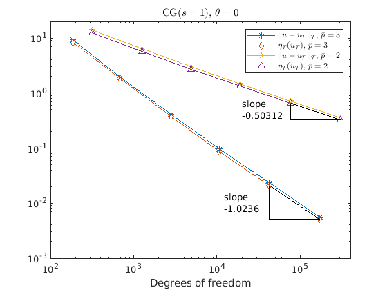
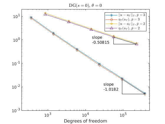
Figure 3. Approximation of the solution $u$ to the HJBI problem (4.1) via the $C^{0}$-IP (top) and DG (bottom) schemes under mesh-refinement with polynomial degrees $\bar{p}\in\{2,3\}$. We illustrate the error (4.2) and the a posteriori estimator (4.3) for the approximation $u_{\mathcal{T}}\in V^{s}_{\mathcal{T}}$ to the solution $u$, using $\theta=0$ (left) and $\theta=\frac{1}{2}$ (right).

4.2. Numerical approximation of the effective Hamiltonian

In this numerical experiment, we demonstrate the numerical scheme for the approximation of the effective Hamiltonian corresponding to the HJBI operator

$$F:\mathbb{R}^{2}\times\mathbb{R}^{2\times 2}_{\mathrm{sym}}\rightarrow\mathbb{R},\qquad F(y,R):=\inf_{\alpha\in\mathcal{A}}\sup_{\beta\in\mathcal{B}}\left\{-A^{\alpha\beta}(y):R-1\right\}$$ (4.4)

with $\mathcal{A}:=[1,2]$, $\mathcal{B}:=[0,1]$, and the coefficient $A=A(y,\alpha,\beta):\mathbb{R}^{2}\times\mathcal{A}\times\mathcal{B}\rightarrow\mathbb{R}^{2\times 2}_{\mathrm{sym}}$ given by

$$A^{\alpha\beta}(y):=\left(a_{0}(y)+\alpha\beta a_{1}(y)\right)B,$$

where we choose positive scalar functions $a_{0},a_{1}:\mathbb{R}^{2}\rightarrow(0,\infty)$ and a symmetric positive definite matrix $B\in\mathbb{R}^{2\times 2}_{\mathrm{sym}}$ defined by

$$B:=\begin{pmatrix}2&-1\\ -1&4\end{pmatrix},\qquad a_{0}\equiv 1,\qquad a_{1}(y):=\sin^{2}(2\pi y_{1})\cos^{2}(2\pi y_{2})+1.$$

It is straightforward to check that this problem fits into the framework of Section 3.1.1 and in particular we have that the Cordes condition (3.4) holds with $\lambda=\frac{1}{4}$. This HJBI operator is chosen so that we know the effective Hamiltonian explicitly.

Remark 4.2.

It can be checked that the HJBI operator (4.4) can be rewritten as HJB operator

$$F(y,R)=\sup_{\beta\in\mathcal{B}}\left\{-\left(a_{0}(y)+\beta a_{1}(y)\right)B:R-1\right\},\qquad(y,R)\in\mathbb{R}^{2}\times\mathbb{R}^{2\times 2}_{\mathrm{sym}},$$

for which the effective Hamiltonian $H:\mathbb{R}^{2\times 2}_{\mathrm{sym}}\rightarrow\mathbb{R}$ is known explicitly and given by

$$H(R):=\max\left\{-\left(\int_{Y}\frac{1}{a_{0}}\right)^{-1}B:R-1,-\left(\int_{Y}\frac{1}{a_{0}+a_{1}}\right)^{-1}B:R-1\right\}$$

for $R\in\mathbb{R}^{2\times 2}_{\mathrm{sym}}$; see [20].

We make it our goal to approximate the effective Hamiltonian $H(R)$ at the point

$$R:=\begin{pmatrix}-2&1\\ 1&-3\end{pmatrix},$$

noting that the same problem was already used for the numerical experiments in [24]. As we have $B:R=-18<0$, the true effective Hamiltonian at this chosen point can be computed as

$$H(R)=-\left(\int_{Y}\frac{1}{a_{0}+a_{1}}\right)^{-1}B:R-1=\frac{9\sqrt{6}\pi}{K(\frac{1}{3})}-1\approx 38.9429127,$$ (4.5)

where $K$ denotes the complete elliptic integral of the first kind.

In our numerical experiments, we approximate the true value of the effective Hamiltonian $H(R)$ from (4.5) by $H_{\mathcal{T}}^{\sigma}(R)$ as defined in (3.9), where we use the $C^{0}$-IP finite element method ($s=1$) with $\theta=\frac{1}{2}$ to obtain the approximation $v_{\mathcal{T}}^{\sigma}(\cdot\,;R)$ to the solution $v^{\sigma}(\cdot\,;R)$ of the cell $\sigma$-problem as described in Section 3.2. We denote the relative approximation error by

$$E_{\mathcal{T}}^{\sigma}:=\frac{\lvert H_{\mathcal{T}}^{\sigma}(R)-H(R)\rvert}{\lvert H(R)\rvert},\qquad H_{\mathcal{T}}^{\sigma}(R):=-\sigma\int_{Y}v_{\mathcal{T}}^{\sigma}(\cdot\,;R)$$

and further write

$$E^{\sigma}:=\frac{\lvert H^{\sigma}(R)-H(R)\rvert}{\lvert H(R)\rvert},\qquad H^{\sigma}(R):=-\sigma\int_{Y}v^{\sigma}(\cdot\,;R).$$

Let us point out that the approximate corrector $v^{\sigma}(\cdot\,;R)$ and consequently the value of $E^{\sigma}$ is not known exactly, but we expect that $E^{\sigma}=\mathcal{O}(\sigma)$ from Remark 3.2.

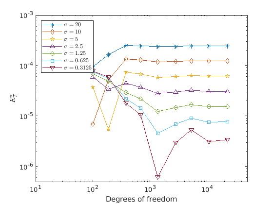
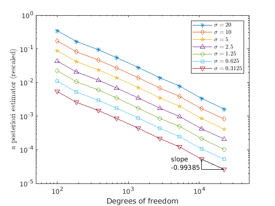
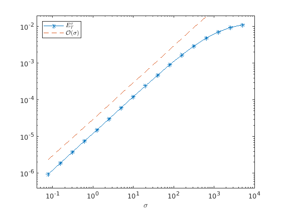
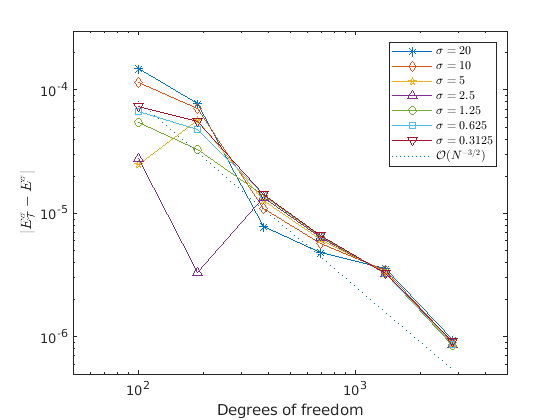
Figure 4. Top: Relative error $E_{\mathcal{T}}^{\sigma}$ (left) and rescaled a posteriori error estimator (right) for fixed $\sigma$ under mesh-refinement using $\bar{p}=3$. Bottom: Relative error $E_{\mathcal{T}}^{\sigma}$ using a fixed discretization with $\bar{p}=20$ (left), and illustration of the speed of convergence of $E_{\mathcal{T}}^{\sigma}$ to $E^{\sigma}$ for fixed $\sigma$ under mesh-refinement using $\bar{p}=3$ (right).

Figure 4 (top) shows the behavior of the relative approximation error $E_{\mathcal{T}}^{\sigma}$ under uniform mesh-refinement for fixed values of $\sigma$, and the corresponding a posteriori error estimator $\eta_{\mathcal{T}}(v_{\mathcal{T}}^{\sigma})$ (re-scaled by a multiplicative constant $C_{\sigma}$ for illustration purposes) using polynomial degree $\bar{p}=3$. We observe that $E_{\mathcal{T}}^{\sigma}$ converges to a constant, namely $E^{\sigma}$, and that the a posteriori estimator is of order $\mathcal{O}(N^{-1})$ as expected, where $N$ denotes the degrees of freedom. In particular, let us emphasize that this is the expected behavior and that the relative error for large numbers of degrees of freedom is entirely dominated by the $\sigma$-error $E^{\sigma}$.

Figure 4 (bottom) illustrates accurate approximations to the unknown values $E^{\sigma}$ for various values of the parameter $\sigma$, and the convergence rate for the convergence of $E_{\mathcal{T}}^{\sigma}$ to the value $E^{\sigma}$. The accurate approximations to the values $E^{\sigma}$ are obtained using high polynomial degree $\bar{p}=20$ and a fixed triangulation (longest edge $\sqrt{2}\times 2^{-3}$), and we observe convergence of order $\mathcal{O}(\sigma)$ as $\sigma$ tends to zero, as expected. Let us note that it is difficult to obtain accurate approximations for extremely small values of $\sigma$ as those lead to poorly conditioned discrete problems. We further observe that $\lvert E_{\mathcal{T}}^{\sigma}-E^{\sigma}\rvert$ is of order $\mathcal{O}(N^{-\frac{3}{2}})$ for fixed $\sigma$, where we take the unknown value $E^{\sigma}$ to be the previously obtained accurate approximation. This rate is higher than predicted by Remark 3.2, which is based on an error estimate in the $\|\cdot\|_{\mathcal{T},\lambda_{\sigma}}$-norm and is therefore indeed expected to overestimate the error between $H_{\mathcal{T}}^{\sigma}(R)$ and $H(R)$ related to the weaker integral functional from (3.9).

5. Conclusion

In this work we introduced discontinuous Galerkin and $C^{0}$ interior penalty finite element schemes for the numerical approximation of periodic HJBI problems with an application to the approximation of effective Hamiltonians to ergodic HJBI operators. The first part of this paper was focused on periodic HJBI cell problems and we have performed rigorous a posteriori and a priori error analyses for a wide class of numerical schemes. In particular, the a posteriori analysis was independent of the choice of numerical scheme. The second part of this paper was focused on the approximation of the effective Hamiltonian corresponding to ergodic HJBI operators. An approximation scheme for the effective Hamiltonian via a DG/$C^{0}$-IP approximation to approximate correctors was presented and rigorously analyzed. Finally, we presented numerical experiments illustrating the theoretical results and the performance of the numerical schemes.

References

- [1] Y. Achdou, F. Camilli, and I. Capuzzo Dolcetta. Homogenization of Hamilton-Jacobi equations: numerical methods. Math. Models Methods Appl. Sci., 18(7):1115–1143, 2008.
- [2] O. Alvarez and M. Bardi. Viscosity solutions methods for singular perturbations in deterministic and stochastic control. SIAM J. Control Optim., 40(4):1159–1188, 2001.
- [3] O. Alvarez and M. Bardi. Singular perturbations of nonlinear degenerate parabolic PDEs: a general convergence result. Arch. Ration. Mech. Anal., 170(1):17–61, 2003.
- [4] O. Alvarez and M. Bardi. Ergodic problems in differential games. In Advances in dynamic game theory, volume 9 of Ann. Internat. Soc. Dynam. Games, pages 131–152. Birkhäuser Boston, Boston, MA, 2007.
- [5] O. Alvarez and M. Bardi. Ergodicity, stabilization, and singular perturbations for Bellman-Isaacs equations. Mem. Amer. Math. Soc., 204(960):vi+77, 2010.
- [6] O. Alvarez, M. Bardi, and C. Marchi. Multiscale problems and homogenization for second-order Hamilton-Jacobi equations. J. Differential Equations, 243(2):349–387, 2007.
- [7] M. Arisawa and P.-L. Lions. On ergodic stochastic control. Comm. Partial Differential Equations, 23(11-12):2187–2217, 1998.
- [8] S. C. Brenner and E. L. Kawecki. Adaptive interior penalty methods for Hamilton–Jacobi–Bellman equations with Cordes coefficients. J. Comput. Appl. Math., 388:113241, 17, 2021.
- [9] L. Caffarelli, M. G. Crandall, M. Kocan, and A. Swiech. On viscosity solutions of fully nonlinear equations with measurable ingredients. Comm. Pure Appl. Math., 49(4):365–397, 1996.
- [10] F. Camilli and M. Falcone. An approximation scheme for the optimal control of diffusion processes. RAIRO Modél. Math. Anal. Numér., 29(1):97–122, 1995.
- [11] F. Camilli and E. R. Jakobsen. A finite element like scheme for integro-partial differential Hamilton-Jacobi-Bellman equations. SIAM J. Numer. Anal., 47(4):2407–2431, 2009.
- [12] F. Camilli and C. Marchi. Rates of convergence in periodic homogenization of fully nonlinear uniformly elliptic PDEs. Nonlinearity, 22(6):1481–1498, 2009.
- [13] Y. Capdeboscq, T. Sprekeler, and E. Süli. Finite element approximation of elliptic homogenization problems in nondivergence-form. ESAIM Math. Model. Numer. Anal., 54(4):1221–1257, 2020.
- [14] M. G. Crandall, H. Ishii, and P.-L. Lions. User’s guide to viscosity solutions of second order partial differential equations. Bull. Amer. Math. Soc. (N.S.), 27(1):1–67, 1992.
- [15] L. C. Evans. The perturbed test function method for viscosity solutions of nonlinear PDE. Proc. Roy. Soc. Edinburgh Sect. A, 111(3-4):359–375, 1989.
- [16] L. C. Evans. Periodic homogenisation of certain fully nonlinear partial differential equations. Proc. Roy. Soc. Edinburgh Sect. A, 120(3-4):245–265, 1992.
- [17] M. Falcone and M. Rorro. On a variational approximation of the effective Hamiltonian. In Numerical mathematics and advanced applications, pages 719–726. Springer, Berlin, 2008.
- [18] X. Feng, R. Glowinski, and M. Neilan. Recent developments in numerical methods for fully nonlinear second order partial differential equations. SIAM Rev., 55(2):205–267, 2013.
- [19] X. Feng and M. Jensen. Convergent semi-Lagrangian methods for the Monge–Ampère equation on unstructured grids. SIAM J. Numer. Anal., 55(2):691–712, 2017.
- [20] C. Finlay and A. M. Oberman. Approximate homogenization of convex nonlinear elliptic PDEs. Commun. Math. Sci., 16(7):1895–1906, 2018.
- [21] C. Finlay and A. M. Oberman. Approximate homogenization of fully nonlinear elliptic PDEs: estimates and numerical results for Pucci type equations. J. Sci. Comput., 77(2):936–949, 2018.
- [22] W. H. Fleming and H. M. Soner. Controlled Markov processes and viscosity solutions, volume 25 of Stochastic Modelling and Applied Probability. Springer, New York, second edition, 2006.
- [23] D. Gallistl. Numerical approximation of planar oblique derivative problems in nondivergence form. Math. Comp., 88(317):1091–1119, 2019.
- [24] D. Gallistl, T. Sprekeler, and E. Süli. Mixed finite element approximation of periodic Hamilton–Jacobi–Bellman problems with application to numerical homogenization. Multiscale Model. Simul., 2021 (Forthcoming article).
- [25] D. Gallistl and E. Süli. Mixed finite element approximation of the Hamilton-Jacobi-Bellman equation with Cordes coefficients. SIAM J. Numer. Anal., 57(2):592–614, 2019.
- [26] R. Glowinski, S. Leung, and J. Qian. A simple explicit operator-splitting method for effective Hamiltonians. SIAM J. Sci. Comput., 40(1):A484–A503, 2018.
- [27] D. A. Gomes and A. M. Oberman. Computing the effective Hamiltonian using a variational approach. SIAM J. Control Optim., 43(3):792–812, 2004.
- [28] H. Ishii. On uniqueness and existence of viscosity solutions of fully nonlinear second-order elliptic PDEs. Comm. Pure Appl. Math., 42(1):15–45, 1989.
- [29] M. Jensen. finite element convergence for degenerate isotropic Hamilton-Jacobi-Bellman equations. IMA J. Numer. Anal., 37(3):1300–1316, 2017.
- [30] M. Jensen and I. Smears. On the convergence of finite element methods for Hamilton-Jacobi-Bellman equations. SIAM J. Numer. Anal., 51(1):137–162, 2013.
- [31] O. A. Karakashian and F. Pascal. A posteriori error estimates for a discontinuous Galerkin approximation of second-order elliptic problems. SIAM J. Numer. Anal., 41(6):2374–2399, 2003.
- [32] E. L. Kawecki. A DGFEM for nondivergence form elliptic equations with Cordes coefficients on curved domains. Numer. Methods Partial Differential Equations, 35(5):1717–1744, 2019.
- [33] E. L. Kawecki. A discontinuous Galerkin finite element method for uniformly elliptic two dimensional oblique boundary-value problems. SIAM J. Numer. Anal., 57(2):751–778, 2019.
- [34] E. L. Kawecki, O. Lakkis, and T. Pryer. A finite element method for the Monge–Ampère equation with transport boundary conditions. arXiv preprint arXiv:1807.03535, 2018.
- [35] E. L. Kawecki and T. Pryer. Virtual element methods for non-divergence form equations. To appear.
- [36] E. L. Kawecki and I. Smears. Unified analysis of discontinuous Galerkin and -interior penalty finite element methods for Hamilton-Jacobi-Bellman and Isaacs equations. ESAIM Math. Model. Numer. Anal., 55(2):449–478, 2021.
- [37] E. L. Kawecki and I. Smears. Convergence of adaptive discontinuous Galerkin and -interior penalty finite element methods for Hamilton-Jacobi-Bellman and Isaacs equations. Found. Comput. Math., 2021. doi:10.1007/s10208-021-09493-0.
- [38] P.-L. Lions. Optimal control of diffusion processes and Hamilton-Jacobi-Bellman equations. II. Viscosity solutions and uniqueness. Comm. Partial Differential Equations, 8(11):1229–1276, 1983.
- [39] P.-L. Lions. A remark on Bony maximum principle. Proc. Amer. Math. Soc., 88(3):503–508, 1983.
- [40] S. Luo, Y. Yu, and H. Zhao. A new approximation for effective Hamiltonians for homogenization of a class of Hamilton-Jacobi equations. Multiscale Model. Simul., 9(2):711–734, 2011.
- [41] M. Neilan, A. J. Salgado, and W. Zhang. Numerical analysis of strongly nonlinear PDEs. Acta Numer., 26:137–303, 2017.
- [42] M. Neilan and M. Wu. Discrete Miranda-Talenti estimates and applications to linear and nonlinear PDEs. J. Comput. Appl. Math., 356:358–376, 2019.
- [43] A. M. Oberman, R. Takei, and A. Vladimirsky. Homogenization of metric Hamilton-Jacobi equations. Multiscale Model. Simul., 8(1):269–295, 2009.
- [44] J. Qian. Two approximations for effective Hamiltonians arising from homogenization of Hamilton-Jacobi equations. UCLA CAM report 03–39, 2003.
- [45] J. Qian, H. V. Tran, and Y. Yu. Min-max formulas and other properties of certain classes of nonconvex effective Hamiltonians. Math. Ann., 372(1-2):91–123, 2018.
- [46] A. J. Salgado and W. Zhang. Finite element approximation of the Isaacs equation. ESAIM Math. Model. Numer. Anal., 53(2):351–374, 2019.
- [47] J. Schöberl. C++ 11 implementation of finite elements in ngsolve. Tech. Rep. ASC Report 30/2014, Institute for Analysis and Scientific Computing, Vienna University of Technology, 2014.
- [48] I. Smears and E. Süli. Discontinuous Galerkin finite element approximation of nondivergence form elliptic equations with Cordès coefficients. SIAM J. Numer. Anal., 51(4):2088–2106, 2013.
- [49] I. Smears and E. Süli. Discontinuous Galerkin finite element approximation of Hamilton-Jacobi-Bellman equations with Cordes coefficients. SIAM J. Numer. Anal., 52(2):993–1016, 2014.
- [50] I. Smears and E. Süli. Discontinuous Galerkin finite element methods for time-dependent Hamilton-Jacobi-Bellman equations with Cordes coefficients. Numer. Math., 133(1):141–176, 2016.
- [51] T. Sprekeler and H. V. Tran. Optimal convergence rates for elliptic homogenization problems in nondivergence-form: analysis and numerical illustrations, arXiv:2009.11259 [math.AP].
- [52] K. Vemaganti. Discontinuous Galerkin methods for periodic boundary value problems. Numer. Methods Partial Differential Equations, 23(3):587–596, 2007.